Loughborough UniversityInstitutional Repository

Cell-signalling repression inbacterial quorum sensing

This item was submitted to Loughborough University's Institutional Repositoryby the/an author.

Additional Information:

• This is a pre-copy-editing, author-produced PDF of an article acceptedfor publication in Mathematical Medicine and Biology [ c© Oxford Univer-sity Press] following peer review. The definitive publisher-authenticatedversion: WARD, J.R., KING, J.P., KOERBER, A.J., CROFT, A.M.,SOCKETT, R.E. and WILLIAMS, P., 2004. Cell-signalling repression inbacterial quorum sensing. Mathematical Medicine and Biology, 21(3) pp.169-204, is available online at: http://intl-imammb.oxfordjournals.org/.

Metadata Record: https://dspace.lboro.ac.uk/2134/314

Please cite the published version.

Cell-signalling repression in bacterial quorum

sensing

J.P. Ward∗,

Mathematical Biology Group, Department of Mathematical Sciences, Loughborough University,

Loughborough, LE11 3TU, UK.

J.R. King, A.J. Koerber,

Division of Theoretical Mechanics, School of Mathematical Sciences,

University of Nottingham, Nottingham, NG7 2RD, UK.

J.M. Croft, R.E. Sockett,

Division of Genetics, School of Clinical Laboratory Sciences, Queens Medical Centre,

University of Nottingham, Nottingham, NG7 2UH, UK.

and

P. Williams,

School of Pharmaceutical Sciences, University of Nottingham, Nottingham, NG7 2RD, UK.

Abstract

In this paper we expand on two mathematical models for investigating the role of three

distinct repression mechanisms within the so called quorum sensing (QS) cell-signalling

process of bacterial colonies growing (1) in liquid cultures and (2) in biofilms. The repres-

sion mechanisms studied are (i) reduction of cell signalling molecule (QSM) production by

a constitutively produced agent degrading the messenger RNA of a crucial enzyme (QSE),

(ii) lower QSM production rate due to a negative feedback process and (iii) loss of QSMs by

binding directly to a constitutively produced agent; the first two mechanisms are known to

be employed by the pathogenic bacterium Pseudomonas aeruginosa and the last is relevant

to the plant pathogen Agrobacterium tumefaciens. The modelling approach assumes that

the bacterial colony consists of two sub-populations, namely down- and up-regulated cells,

that differ in the rates at which they produce QSMs, while QSM concentration governs

the switching between sub-populations. Parameter estimates are obtained by curve-fitting

experimental data (involving P. aeruginosa growth in liquid culture, obtained as part of

this study) to solutions of model (1). Asymptotic analysis of the model (1) shows that

mechanism (i) is necessary, but not sufficient, to predict the observed saturation of QSM

levels in an exponentially growing colony; either mechanism (ii) or (iii) also needs to be

incorporated to obtain saturation. Consequently, only a fraction of the population will be-

come up-regulated. Furthermore, only mechanisms (i) and (iii) effect the main timescales

for up regulation. Repression was found to play less significant role in a biofilms, but

mechanisms (i)-(iii) were nevertheless found to reduce the ulitimate up-regulated cell frac-

tion and mechanisms (i) and (iii) increase the timescale for substantial up regulation and

decrease the wave speed of an expanding front of QS activity.

Keywords: bacteria; quorum sensing; repression; mathematical modelling; parameter esti-

mation.

∗Author to whom correspondence should be addressed. Email: john.ward@lboro.ac.uk

1

1 Introduction

The phenomenon of quorum sensing (QS), a sophisticated cell-to-cell signalling system em-

ployed by many bacterial species, is emerging as one of the most important issues in the study

of bacterial behavioural dynamics [19]. The phenomenon manifests itself in the apparent

change of the behaviour (phenotype) of an entire population when the bacterial density has

reached a threshold level. Such density dependent behavioural changes include the “switching

on” of bioluminescence of Vibrio fischeri (a species that resides in certain deep sea squid, [11]),

conjugal transfer in Agrobacterium tumefaciens (a form of sexual reproduction, [22]), swarm-

ing behaviour in Serratia liquefacians (presumably as a means of population expansion) and

production of virulence factors in Burkholderia cepacia and Pseudomonas aeruginosa (both

with significant medical implications for sufferers of cystic fibrosis [10] and, in the latter case,

for patients with severe open wounds or burn injuries [14]). In some cases, rather than QS

“switching on” a given phenotype, it may instead function by de-repressing a phenotype which

is actively repressed at low densities [2, 17]. The advantage of QS for the bacteria is that by

restricting certain behavioural traits it reduces expenditure of vital nutrient resources on activ-

ities that will have no impact when the population density is small. In the case of the infection

of wounds by P. aeruginosa, it is believed that QS enables the initially benign colonising bac-

teria to build up numbers whilst being (relatively) overlooked by the immune system; when

the population finally becomes virulent, their greater numbers thus increase the chances of

the immune system being overwhelmed, leading to a serious infection.

In its “simplest” form, QS is governed by two genes, one encoding an enzyme (QSE) that

promotes the production of a small, freely diffusible quorum sensing molecule (QSM) and the

other a cognate quorum sensing protein (QSP) [24]. A QSM can combine with a QSP to

form a QSM-QSP complex which, by interacting with the promoter region of the gene (called

the lux-box), enhances production of the QSM, and perhaps of the QSP, and up regulates

the production of proteins that are involved in the appropriate shift in behavioural traits (for

example, production of luciferase in V. fischeri to produce bioluminescence). Consequently,

as the bacterial density increases, more QSM will be present, leading to greater up regulation

of the appropriate genes within the population. That is to say, QS is a partially autoinductive

process involving positive feedback loops; by “partially” we mean here that the production of

QS products is limited by the number of bacteria and availability of raw materials. Figure

1 is a simple schematic of the LasR/LasI (primary) QS system of P. aeruginosa based on Fig. 1

Withers et al. [27]; here the protein LasR is a QSP and 3-oxo-C12-HSL (N-[3-oxododecanoyl]-

L-homoserine lactone) is a QSM. Such autoinductive systems could bring about the needless

over-production of QSMs, QSPs and other up regulated products, leading to waste in nutrient

resources. Discoveries in recent years have shown that a few species have evolved means of

bypassing this problem, by repressing certain components of the QS process. The most well

studied examples are those of P. aeruginosa [6, 7, 8, 21] and A. tumefaciens [4, 23]. The

repression mechanisms investigated in this paper are summarised below, the first two being

known to be relevant for P. aeruginosa and the last to A. tumefaciens.

1. “Background” Inhibition (BI) of QSM output by constitutively produced regulator pro-

teins which interfere in some way with the production or action of the QSE (which

catalyses the reaction of the QSM precursors). Two such proteins have been identified

in P. aeruginosa, namely QscR [6] and RsmA [21], which are produced independently

2

of QS; see Figure 1. RsmA is believed to destroy messenger-RNA transcripts for many

proteins [13], including that for the enzyme LasI, the QSE for the QSM 3-oxo-C12-HSL

in P. aeruginosa (see Figure 2); how QscR inhibit QSM output is currently unknown. Fig. 2

2. Negative feedback (NF) process, whereby a protein positively regulated by QS represses

QSM production. In P. aeruginosa the production of repressor protein RsaL is enhanced

by QS; this protein probably binds directly to the lasI promoter, preventing expression

of the gene [7] (see Figure 1).

3. “Soaking up” (SU) of QSMs by forming inert dimers with certain constitutively pro-

duced proteins. The protein TrlR in A. tumefaciens is structural similar to the bac-

terium’s QSP (namely TraR) and can bind with a QSM to form a stable dimer [4],

rendering the QSM unavailable for QS. In fact, the role of TrlR seems to be considerably

more complex, as it can also bind with and thus deactivate QSPs; however, only the

action of the soaking up of QSMs will be considered in this paper.

The abbreviations BI, NF and SU for the three repression mechanism will be used throughout

the paper. A. tumefaciens produces at least one other molecule involved in the repression

of QS, namely TraM [23], which also deactivates the QSP molecule. Curiously, QS seems to

promote the production of both TraR and TraM. This apparent conflict between promotion

and repression suggests that there are other, as yet undiscovered, regulators involved, perhaps

processes that somehow delay the production of TraM. Since the details of how TraR, TraM

and TrlR are regulated and interact is open to speculation, the process of QSP repression will

not be considered in this paper.

As is now widely recognised, at the intracellular level many biological phenomena are

governed by complex interactions between positive and negative feedback processes. Here

we consider in detail a relatively well-characterised example which has significant medical (in

particular) implications. Specifically, we consider cell signalling processes in a population of

bacteria whereby positive feedback (quorum sensing) leads to concerted action by the entire

colony, but negative feedback (repression) is needed if this concerted action is not to lead

to excessive use of available resources. By operating in tandem, the two processes allow the

colony to operate in an efficient multi-cellular fashion.

The QS process has been the subject of a number mathematical models, the approaches

ranging competition models [3], through mass-action-based kinetic models of the biochem-

istry [5, 9, 15, 18] to macro-scale population models [16, 25, 26]. The mass action model

of Dockery and Keener [9], modelling QS in P. aeruginosa is (more-or-less) as depicted in

Figure 1, considered, inter alia, (a) the decay of the mRNA-lasI protein required to generate

QSMs, reflecting the BI mechanism, (b) an inhibitor of mRNA-lasI, reflecting NF, and (c) the

constant decay of QSMs, reflecting SU; we note, however, that there is no biological evidence

that P. aeruginosa produces a molecule that soaks-up or cause decay of QSMs, so it is uncer-

tain whether the SU process is relevant for this bacterium. The role of these QS repression

mechanisms was not investigated systematically in [9], indeed, the negative feedback loop was

neglected in order to simplify the model for further analysis; consequently no investigation

into the role of feedback was attempted. The approach to the modelling in the current paper

studies QS on a macroscopic level, extending the model of Ward et al. [26]. The modelling

assumes that the bacteria are in one of two states, namely down-regulated and up-regulated,

with QSM levels controlling the rates of conversion from one form to the other. The addition

3

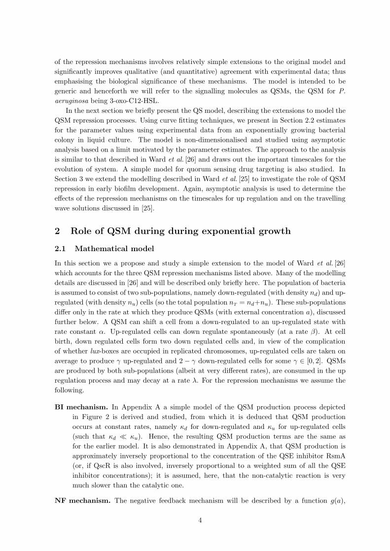
of the repression mechanisms involves relatively simple extensions to the original model and

significantly improves qualitative (and quantitative) agreement with experimental data; thus

emphasising the biological significance of these mechanisms. The model is intended to be

generic and henceforth we will refer to the signalling molecules as QSMs, the QSM for P.

aeruginosa being 3-oxo-C12-HSL.

In the next section we briefly present the QS model, describing the extensions to model the

QSM repression processes. Using curve fitting techniques, we present in Section 2.2 estimates

for the parameter values using experimental data from an exponentially growing bacterial

colony in liquid culture. The model is non-dimensionalised and studied using asymptotic

analysis based on a limit motivated by the parameter estimates. The approach to the analysis

is similar to that described in Ward et al. [26] and draws out the important timescales for the

evolution of system. A simple model for quorum sensing drug targeting is also studied. In

Section 3 we extend the modelling described in Ward et al. [25] to investigate the role of QSM

repression in early biofilm development. Again, asymptotic analysis is used to determine the

effects of the repression mechanisms on the timescales for up regulation and on the travelling

wave solutions discussed in [25].

2 Role of QSM during during exponential growth

2.1 Mathematical model

In this section we a propose and study a simple extension to the model of Ward et al. [26]

which accounts for the three QSM repression mechanisms listed above. Many of the modelling

details are discussed in [26] and will be described only briefly here. The population of bacteria

is assumed to consist of two sub-populations, namely down-regulated (with density nd) and up-

regulated (with density nu) cells (so the total population nT = nd+nu). These sub-populations

differ only in the rate at which they produce QSMs (with external concentration a), discussed

further below. A QSM can shift a cell from a down-regulated to an up-regulated state with

rate constant α. Up-regulated cells can down regulate spontaneously (at a rate β). At cell

birth, down regulated cells form two down regulated cells and, in view of the complication

of whether lux-boxes are occupied in replicated chromosomes, up-regulated cells are taken on

average to produce γ up-regulated and 2 − γ down-regulated cells for some γ ∈ [0, 2]. QSMs

are produced by both sub-populations (albeit at very different rates), are consumed in the up

regulation process and may decay at a rate λ. For the repression mechanisms we assume the

following.

BI mechanism. In Appendix A a simple model of the QSM production process depicted

in Figure 2 is derived and studied, from which it is deduced that QSM production

occurs at constant rates, namely κd for down-regulated and κu for up-regulated cells

(such that κd κu). Hence, the resulting QSM production terms are the same as

for the earlier model. It is also demonstrated in Appendix A, that QSM production is

approximately inversely proportional to the concentration of the QSE inhibitor RsmA

(or, if QscR is also involved, inversely proportional to a weighted sum of all the QSE

inhibitor concentrations); it is assumed, here, that the non-catalytic reaction is very

much slower than the catalytic one.

NF mechanism. The negative feedback mechanism will be described by a function g(a),

4

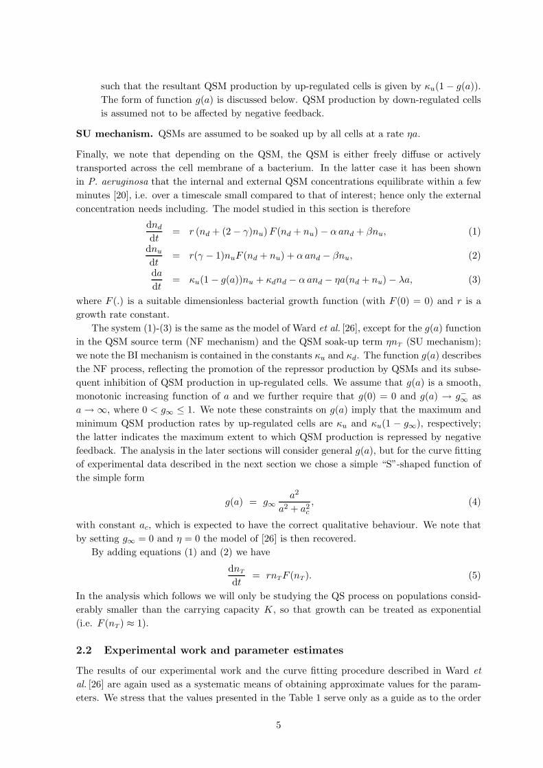
such that the resultant QSM production by up-regulated cells is given by κu(1 − g(a)).

The form of function g(a) is discussed below. QSM production by down-regulated cells

is assumed not to be affected by negative feedback.

SU mechanism. QSMs are assumed to be soaked up by all cells at a rate ηa.

Finally, we note that depending on the QSM, the QSM is either freely diffuse or actively

transported across the cell membrane of a bacterium. In the latter case it has been shown

in P. aeruginosa that the internal and external QSM concentrations equilibrate within a few

minutes [20], i.e. over a timescale small compared to that of interest; hence only the external

concentration needs including. The model studied in this section is therefore

dnd

dt= r (nd + (2 − γ)nu)F (nd + nu) − αand + βnu, (1)

dnu

dt= r(γ − 1)nuF (nd + nu) + αand − βnu, (2)

da

dt= κu(1 − g(a))nu + κdnd − αand − ηa(nd + nu) − λa, (3)

where F (.) is a suitable dimensionless bacterial growth function (with F (0) = 0) and r is a

growth rate constant.

The system (1)-(3) is the same as the model of Ward et al. [26], except for the g(a) function

in the QSM source term (NF mechanism) and the QSM soak-up term ηnT (SU mechanism);

we note the BI mechanism is contained in the constants κu and κd. The function g(a) describes

the NF process, reflecting the promotion of the repressor production by QSMs and its subse-

quent inhibition of QSM production in up-regulated cells. We assume that g(a) is a smooth,

monotonic increasing function of a and we further require that g(0) = 0 and g(a) → g−∞ as

a → ∞, where 0 < g∞ ≤ 1. We note these constraints on g(a) imply that the maximum and

minimum QSM production rates by up-regulated cells are κu and κu(1 − g∞), respectively;

the latter indicates the maximum extent to which QSM production is repressed by negative

feedback. The analysis in the later sections will consider general g(a), but for the curve fitting

of experimental data described in the next section we chose a simple “S”-shaped function of

the simple form

g(a) = g∞a2

a2 + a2c

, (4)

with constant ac, which is expected to have the correct qualitative behaviour. We note that

by setting g∞ = 0 and η = 0 the model of [26] is then recovered.

By adding equations (1) and (2) we have

dnTdt

= rnTF (nT ). (5)

In the analysis which follows we will only be studying the QS process on populations consid-

erably smaller than the carrying capacity K, so that growth can be treated as exponential

(i.e. F (nT ) ≈ 1).

2.2 Experimental work and parameter estimates

The results of our experimental work and the curve fitting procedure described in Ward et

al. [26] are again used as a systematic means of obtaining approximate values for the param-

eters. We stress that the values presented in the Table 1 serve only as a guide as to the order

5

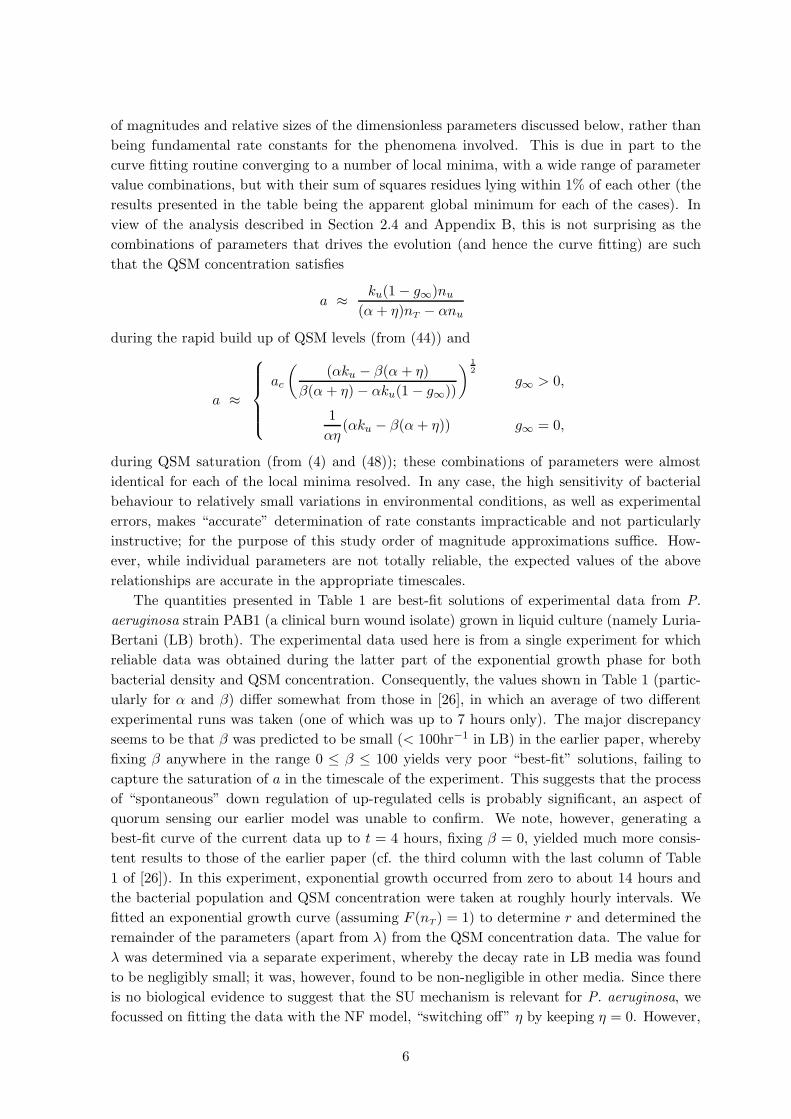
of magnitudes and relative sizes of the dimensionless parameters discussed below, rather than

being fundamental rate constants for the phenomena involved. This is due in part to the

curve fitting routine converging to a number of local minima, with a wide range of parameter

value combinations, but with their sum of squares residues lying within 1% of each other (the

results presented in the table being the apparent global minimum for each of the cases). In

view of the analysis described in Section 2.4 and Appendix B, this is not surprising as the

combinations of parameters that drives the evolution (and hence the curve fitting) are such

that the QSM concentration satisfies

a ≈ ku(1 − g∞)nu

(α+ η)nT − αnu

during the rapid build up of QSM levels (from (44)) and

a ≈

ac

(

(αku − β(α + η)

β(α + η) − αku(1 − g∞))

)12

g∞ > 0,

1

αη(αku − β(α+ η)) g∞ = 0,

during QSM saturation (from (4) and (48)); these combinations of parameters were almost

identical for each of the local minima resolved. In any case, the high sensitivity of bacterial

behaviour to relatively small variations in environmental conditions, as well as experimental

errors, makes “accurate” determination of rate constants impracticable and not particularly

instructive; for the purpose of this study order of magnitude approximations suffice. How-

ever, while individual parameters are not totally reliable, the expected values of the above

relationships are accurate in the appropriate timescales.

The quantities presented in Table 1 are best-fit solutions of experimental data from P.

aeruginosa strain PAB1 (a clinical burn wound isolate) grown in liquid culture (namely Luria-

Bertani (LB) broth). The experimental data used here is from a single experiment for which

reliable data was obtained during the latter part of the exponential growth phase for both

bacterial density and QSM concentration. Consequently, the values shown in Table 1 (partic-

ularly for α and β) differ somewhat from those in [26], in which an average of two different

experimental runs was taken (one of which was up to 7 hours only). The major discrepancy

seems to be that β was predicted to be small (< 100hr−1 in LB) in the earlier paper, whereby

fixing β anywhere in the range 0 ≤ β ≤ 100 yields very poor “best-fit” solutions, failing to

capture the saturation of a in the timescale of the experiment. This suggests that the process

of “spontaneous” down regulation of up-regulated cells is probably significant, an aspect of

quorum sensing our earlier model was unable to confirm. We note, however, generating a

best-fit curve of the current data up to t = 4 hours, fixing β = 0, yielded much more consis-

tent results to those of the earlier paper (cf. the third column with the last column of Table

1 of [26]). In this experiment, exponential growth occurred from zero to about 14 hours and

the bacterial population and QSM concentration were taken at roughly hourly intervals. We

fitted an exponential growth curve (assuming F (nT ) = 1) to determine r and determined the

remainder of the parameters (apart from λ) from the QSM concentration data. The value for

λ was determined via a separate experiment, whereby the decay rate in LB media was found

to be negligibly small; it was, however, found to be non-negligible in other media. Since there

is no biological evidence to suggest that the SU mechanism is relevant for P. aeruginosa, we

focussed on fitting the data with the NF model, “switching off” η by keeping η = 0. However,

6

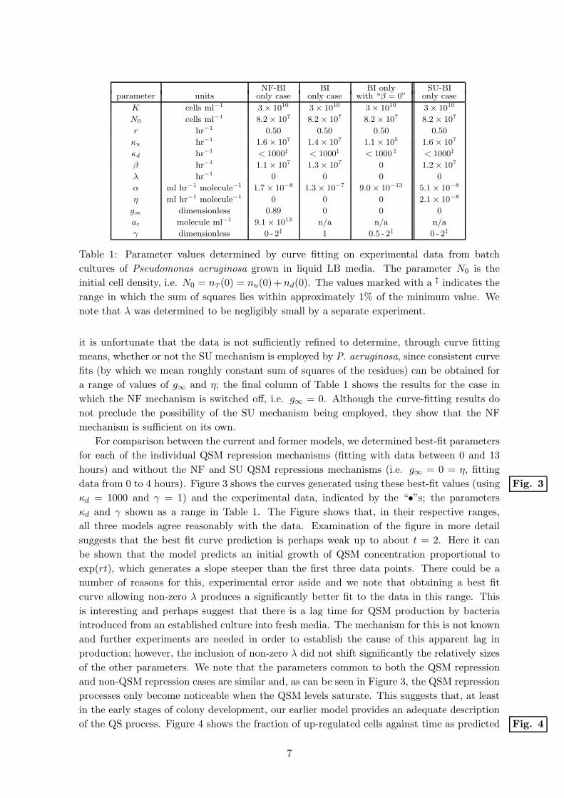
NF-BI BI BI only SU-BIparameter units only case only case with “β = 0” only case

K cells ml−1 3 × 1010 3 × 1010 3 × 1010 3 × 1010

N0 cells ml−1 8.2 × 107 8.2 × 107 8.2 × 107 8.2 × 107

r hr−1 0.50 0.50 0.50 0.50

κu hr−1 1.6 × 107 1.4 × 107 1.1 × 105 1.6 × 107

κd hr−1 < 1000‡ < 1000‡ < 1000 ‡ < 1000‡

β hr−1 1.1 × 107 1.3 × 107 0 1.2 × 107

λ hr−1 0 0 0 0

α ml hr−1 molecule−1 1.7 × 10−8 1.3 × 10−7 9.0 × 10−13 5.1 × 10−8

η ml hr−1 molecule−1 0 0 0 2.1 × 10−8

g∞ dimensionless 0.89 0 0 0

ac molecule ml−1 9.1 × 1013 n/a n/a n/a

γ dimensionless 0 - 2‡ 1 0.5 - 2‡ 0 - 2‡

Table 1: Parameter values determined by curve fitting on experimental data from batch

cultures of Pseudomonas aeruginosa grown in liquid LB media. The parameter N0 is the

initial cell density, i.e. N0 = nT (0) = nu(0) +nd(0). The values marked with a ‡ indicates the

range in which the sum of squares lies within approximately 1% of the minimum value. We

note that λ was determined to be negligibly small by a separate experiment.

it is unfortunate that the data is not sufficiently refined to determine, through curve fitting

means, whether or not the SU mechanism is employed by P. aeruginosa, since consistent curve

fits (by which we mean roughly constant sum of squares of the residues) can be obtained for

a range of values of g∞ and η; the final column of Table 1 shows the results for the case in

which the NF mechanism is switched off, i.e. g∞ = 0. Although the curve-fitting results do

not preclude the possibility of the SU mechanism being employed, they show that the NF

mechanism is sufficient on its own.

For comparison between the current and former models, we determined best-fit parameters

for each of the individual QSM repression mechanisms (fitting with data between 0 and 13

hours) and without the NF and SU QSM repressions mechanisms (i.e. g∞ = 0 = η, fitting

data from 0 to 4 hours). Figure 3 shows the curves generated using these best-fit values (using Fig. 3

κd = 1000 and γ = 1) and the experimental data, indicated by the “•”s; the parameters

κd and γ shown as a range in Table 1. The Figure shows that, in their respective ranges,

all three models agree reasonably with the data. Examination of the figure in more detail

suggests that the best fit curve prediction is perhaps weak up to about t = 2. Here it can

be shown that the model predicts an initial growth of QSM concentration proportional to

exp(rt), which generates a slope steeper than the first three data points. There could be a

number of reasons for this, experimental error aside and we note that obtaining a best fit

curve allowing non-zero λ produces a significantly better fit to the data in this range. This

is interesting and perhaps suggest that there is a lag time for QSM production by bacteria

introduced from an established culture into fresh media. The mechanism for this is not known

and further experiments are needed in order to establish the cause of this apparent lag in

production; however, the inclusion of non-zero λ did not shift significantly the relatively sizes

of the other parameters. We note that the parameters common to both the QSM repression

and non-QSM repression cases are similar and, as can be seen in Figure 3, the QSM repression

processes only become noticeable when the QSM levels saturate. This suggests that, at least

in the early stages of colony development, our earlier model provides an adequate description

of the QS process. Figure 4 shows the fraction of up-regulated cells against time as predicted Fig. 4

7

by the models using the best-fit parameters. The contrast in proportions between the QSM

repression and non-repression cases is explained by the analysis of the Section 2.4.

2.3 Non-dimensionalisation

Before proceeding with the analysis, we non-dimensionalise the system of equations, using the

rescalings of Ward et al. [26], namely

t = t/r, nu = Knu, nT = KnT , a =κuK

ra, F (nT ) = F (nT );

where the quantities with hats denotes dimensionless variables. Using (5) we eliminate nd =

nT − nu and focus on the following dimensionless system

dnT

dt= nT F (nT ), (6)

dnu

dt= (γ − 1)nuF (nT ) + αa(nT − nu) − βnu, (7)

da

dt= nu(1 − g(a)) + ε(nT − nu) − µa(nT − nu) − ηanT − λa, (8)

where ε = κd/κu, α = ακuK/r2, β = β/r, λ = λ/r, η = ηK/r and µ = αK/r; we assume all

parameters in g(a) are also appropriately non-dimensionalised; for example, in (4) we choose

ac = ac r/κuK, where ac = O(10−4). Using the data in Table 1 the approximate order of

magnitudes of the dimensionless parameters are α = O(1010), β = O(107), µ = O(103), λ

negligible and ε 1 (seemingly ε . 10−4). The data in the last column of Table 1 suggests

that η = O(1010); however, whether or not the SU is mechanism relevant for this bacterium is

uncertain. These dimensionless values contrast somewhat with those given in [26]; however,

the relationships of ε µ β α are maintained. For the remainder of this section the

hats on the dimensionless quantities will be dropped for brevity.

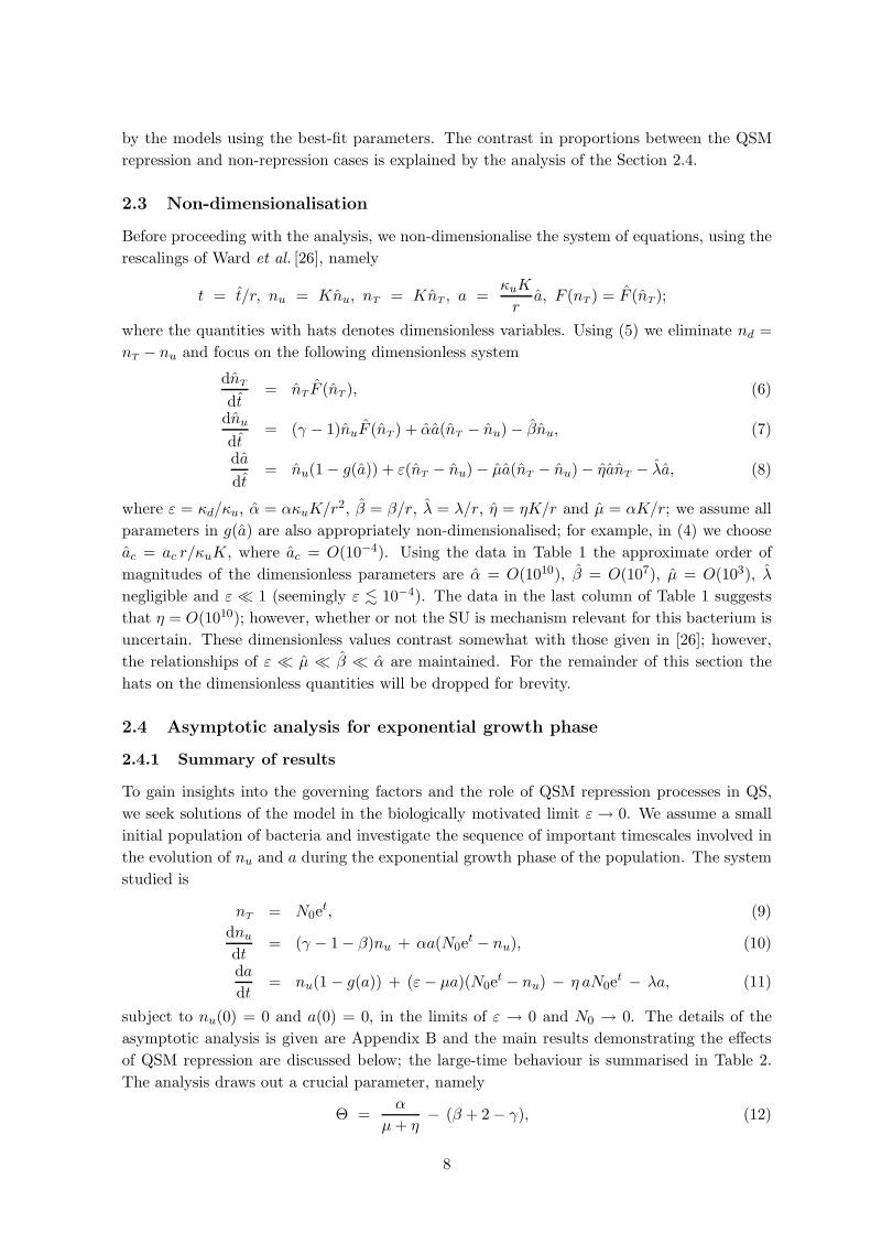
2.4 Asymptotic analysis for exponential growth phase

2.4.1 Summary of results

To gain insights into the governing factors and the role of QSM repression processes in QS,

we seek solutions of the model in the biologically motivated limit ε → 0. We assume a small

initial population of bacteria and investigate the sequence of important timescales involved in

the evolution of nu and a during the exponential growth phase of the population. The system

studied is

nT = N0et, (9)

dnu

dt= (γ − 1 − β)nu + αa(N0e

t − nu), (10)

da

dt= nu(1 − g(a)) + (ε− µa)(N0e

t − nu) − η aN0et − λa, (11)

subject to nu(0) = 0 and a(0) = 0, in the limits of ε → 0 and N0 → 0. The details of the

asymptotic analysis is given are Appendix B and the main results demonstrating the effects

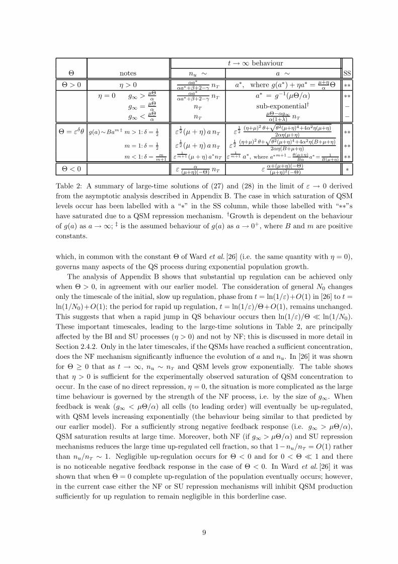
of QSM repression are discussed below; the large-time behaviour is summarised in Table 2.

The analysis draws out a crucial parameter, namely

Θ =α

µ+ η− (β + 2 − γ), (12)

8

t→ ∞ behaviour

Θ notes nu ∼ a ∼ SS

Θ > 0 η > 0 αa∗

αa∗+β+2−γ nT a∗, where g(a∗) + ηa∗ = µ+ηα Θ ∗∗

η = 0 g∞ > µΘα

αa∗

αa∗+β+2−γ nT a∗ = g−1(µΘ/α) ∗∗g∞ = µΘ

α nT sub-exponential† −g∞ < µΘ

α nTµΘ−αg∞α(1+λ) nT −

Θ = εδθ g(a)∼Bam ‡ m > 1: δ = 12

ε12 (µ+ η) anT ε

12

(η+µ)2 θ+√

θ2(µ+η)4+4α2η(µ+η)

2αη(µ+η) ∗∗

m = 1: δ = 12

ε12 (µ+ η) anT ε

12

(η+µ)2 θ+√

θ2(µ+η)4+4α2η(B+µ+η)

2αη(B+µ+η) ∗∗m < 1: δ = m

m+1ε

1m+1 (µ + η) a∗nT ε

1m+1 a∗, where a∗m+1−

θ(µ+η)Bα

a∗ = 1B(µ+η)

∗∗

Θ < 0 ε α(µ+η)(−Θ) nT ε α+(µ+η)(−Θ)

(µ+η)2(−Θ)∗

Table 2: A summary of large-time solutions of (27) and (28) in the limit of ε → 0 derived

from the asymptotic analysis described in Appendix B. The case in which saturation of QSM

levels occur has been labelled with a “∗” in the SS column, while those labelled with “∗∗”shave saturated due to a QSM repression mechanism. †Growth is dependent on the behaviour

of g(a) as a→ ∞; ‡ is the assumed behaviour of g(a) as a→ 0+, where B and m are positive

constants.

which, in common with the constant Θ of Ward et al. [26] (i.e. the same quantity with η = 0),

governs many aspects of the QS process during exponential population growth.

The analysis of Appendix B shows that substantial up regulation can be achieved only

when Θ > 0, in agreement with our earlier model. The consideration of general N0 changes

only the timescale of the initial, slow up regulation, phase from t = ln(1/ε)+O(1) in [26] to t =

ln(1/N0)+O(1); the period for rapid up regulation, t = ln(1/ε)/Θ+O(1), remains unchanged.

This suggests that when a rapid jump in QS behaviour occurs then ln(1/ε)/Θ ln(1/N0).

These important timescales, leading to the large-time solutions in Table 2, are principally

affected by the BI and SU processes (η > 0) and not by NF; this is discussed in more detail in

Section 2.4.2. Only in the later timescales, if the QSMs have reached a sufficient concentration,

does the NF mechanism significantly influence the evolution of a and nu. In [26] it was shown

for Θ ≥ 0 that as t → ∞, nu ∼ nT and QSM levels grow exponentially. The table shows

that η > 0 is sufficient for the experimentally observed saturation of QSM concentration to

occur. In the case of no direct repression, η = 0, the situation is more complicated as the large

time behaviour is governed by the strength of the NF process, i.e. by the size of g∞. When

feedback is weak (g∞ < µΘ/α) all cells (to leading order) will eventually be up-regulated,

with QSM levels increasing exponentially (the behaviour being similar to that predicted by

our earlier model). For a sufficiently strong negative feedback response (i.e. g∞ > µΘ/α),

QSM saturation results at large time. Moreover, both NF (if g∞ > µΘ/α) and SU repression

mechanisms reduces the large time up-regulated cell fraction, so that 1−nu/nT = O(1) rather

than nu/nT ∼ 1. Negligible up-regulation occurs for Θ < 0 and for 0 < Θ 1 and there

is no noticeable negative feedback response in the case of Θ < 0. In Ward et al. [26] it was

shown that when Θ = 0 complete up-regulation of the population eventually occurs; however,

in the current case either the NF or SU repression mechanisms will inhibit QSM production

sufficiently for up regulation to remain negligible in this borderline case.

9

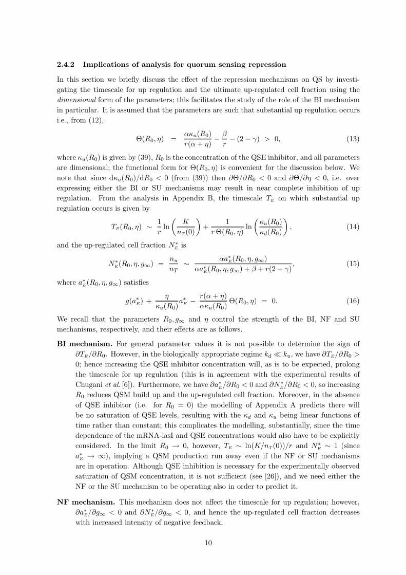
2.4.2 Implications of analysis for quorum sensing repression

In this section we briefly discuss the effect of the repression mechanisms on QS by investi-

gating the timescale for up regulation and the ultimate up-regulated cell fraction using the

dimensional form of the parameters; this facilitates the study of the role of the BI mechanism

in particular. It is assumed that the parameters are such that substantial up regulation occurs

i.e., from (12),

Θ(R0, η) =ακu(R0)

r(α+ η)− β

r− (2 − γ) > 0, (13)

where κu(R0) is given by (39), R0 is the concentration of the QSE inhibitor, and all parameters

are dimensional; the functional form for Θ(R0, η) is convenient for the discussion below. We

note that since dκu(R0)/dR0 < 0 (from (39)) then ∂Θ/∂R0 < 0 and ∂Θ/∂η < 0, i.e. over

expressing either the BI or SU mechanisms may result in near complete inhibition of up

regulation. From the analysis in Appendix B, the timescale TE on which substantial up

regulation occurs is given by

TE(R0, η) ∼ 1

rln

(

K

nT (0)

)

+1

rΘ(R0, η)ln

(

κu(R0)

κd(R0)

)

, (14)

and the up-regulated cell fraction N∗E is

N∗E(R0, η, g∞) =

nu

nT∼ αa∗E(R0, η, g∞)

αa∗E(R0, η, g∞) + β + r(2 − γ), (15)

where a∗E(R0, η, g∞) satisfies

g(a∗E) +η

κu(R0)a∗E − r(α+ η)

ακu(R0)Θ(R0, η) = 0. (16)

We recall that the parameters R0, g∞ and η control the strength of the BI, NF and SU

mechanisms, respectively, and their effects are as follows.

BI mechanism. For general parameter values it is not possible to determine the sign of

∂TE/∂R0. However, in the biologically appropriate regime kd ku, we have ∂TE/∂R0 >

0; hence increasing the QSE inhibitor concentration will, as is to be expected, prolong

the timescale for up regulation (this is in agreement with the experimental results of

Chugani et al. [6]). Furthermore, we have ∂a∗E/∂R0 < 0 and ∂N∗E/∂R0 < 0, so increasing

R0 reduces QSM build up and the up-regulated cell fraction. Moreover, in the absence

of QSE inhibitor (i.e. for R0 = 0) the modelling of Appendix A predicts there will

be no saturation of QSE levels, resulting with the κd and κu being linear functions of

time rather than constant; this complicates the modelling, substantially, since the time

dependence of the mRNA-lasI and QSE concentrations would also have to be explicitly

considered. In the limit R0 → 0, however, TE ∼ ln(K/nT (0))/r and N∗E ∼ 1 (since

a∗E → ∞), implying a QSM production run away even if the NF or SU mechanisms

are in operation. Although QSE inhibition is necessary for the experimentally observed

saturation of QSM concentration, it is not sufficient (see [26]), and we need either the

NF or the SU mechanism to be operating also in order to predict it.

NF mechanism. This mechanism does not affect the timescale for up regulation; however,

∂a∗E/∂g∞ < 0 and ∂N∗E/∂g∞ < 0, and hence the up-regulated cell fraction decreases

with increased intensity of negative feedback.

10

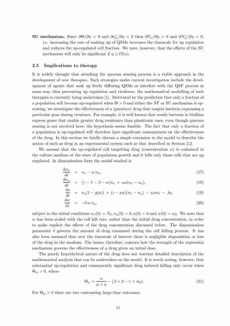
SU mechanism. Since ∂Θ/∂η < 0 and ∂a∗E/∂η < 0 then ∂TE/∂η > 0 and ∂N∗E/∂η < 0,

i.e. increasing the rate of soaking up of QSMs increases the timescale for up regulation

and reduces the up-regulated cell fraction. We note, however, that the effects of the SU

mechanism will only be significant if η ≥ O(α).

2.5 Implications to therapy

It is widely thought that attacking the quorum sensing process is a viable approach in the

development of new therapies. Such strategies under current investigation include the devel-

opment of agents that soak up freely diffusing QSMs or interfere with the QSP process in

some way, thus preventing up regulation and virulence; the mathematical modelling of such

therapies is currently being undertaken [1]. Motivated by the prediction that only a fraction of

a population will become up-regulated when Θ > 0 and either the NF or SU mechanism is op-

erating, we investigate the effectiveness of a (putative) drug that targets bacteria expressing a

particular gene during virulence. For example, it is well known that sessile bacteria in biofilms

express genes that enable greater drug resistance than planktonic ones, even though quorum

sensing is not involved here, the hypothesis seems feasible. The fact that only a fraction of

a population is up-regulated will therefore have significant consequences on the effectiveness

of the drug. In this section we briefly discuss a simple extension to the model to describe the

action of such as drug in an experimental system such as that described in Section 2.2.

We assume that the up-regulated cell targetting drug (concentration w) is contained in

the culture medium at the start of population growth and it kills only those cells that are up

regulated. In dimensionless form the model studied is

dnTdt

= nT − wnu, (17)

dnu

dt= (γ − 1 − β − w)nu + αa(nT − nu), (18)

da

dt= nu(1 − g(a)) + (ε− µa)(nT − nu) − η anT − λa, (19)

dw

dt= −δ w nu, (20)

subject to the initial conditions nT (0) = N0, nu(0) = 0, a(0) = 0 and w(0) = w0. We note that

w has been scaled with the cell kill rate, rather than the initial drug concentration, in order

to make explicit the effects of the drug concentration discussed below. The dimensionless

parameter δ governs the amount of drug consumed during the cell killing process. It has

also been assumed that over the timescale of interest there is negligible degradation or loss

of the drug in the medium. The issues, therefore, concern how the strength of the repression

mechanism governs the effectiveness of a drug given an initial dose.

The purely hypothetical nature of the drug does not warrant detailed description of the

mathematical analysis that can be undertaken on the model. It is worth noting, however, that

substantial up-regulation and consequently significant drug induced killing only occur when

Θw > 0, where

Θw =α

µ+ η− (β + 2 − γ + w0). (21)

For Θw > 0 there are two contrasting large-time outcomes.

11

1. Eventual consumption of the drug, leading ultimately to a resumption of exponential

population growth (and exponential decay of the drug). This outcome requires δ > 0.

2. Sufficient killing of the population that the population ultimately declines exponentially,

with the drug tending to a steady-state, w → w∗ say (note if δ = 0 then w∗ = w0).

It can be shown that a necessary condition for scenario 2. is that w0 ≥ 1.

Figure 5 demonstrates the two large-time outcomes listed above. Here δ = 10, with the Fig. 5

other parameters determined from Table 1 in dimensionless form. The bifurcation between

the two outcomes occurs at w0 ≈ 16.74. We observe that for w0 = 16 there is insufficient drug

to kill off the population, although the dose is sufficiently strong to induce a decline between

t = 5 and t = 20. The drug concentration seems to decay slowly until about t = 40 when there

is a very rapid drop; this corresponds to recovery of growth of the form described in Appendix

B.2.3 leading to w ∼Wc exp(−e(Θ+1)t) (for some constant W ∗c ) during this phase. For w0 = 17

there is sufficient drug that, following an initial non-negligible level of consumption whilst the

population density is of O(0.1), enough remains to prevent population recovery and outcome

2. above ensues. The effects of the NF repression mechanism on the effectiveness of a drug

dose is demonstrated in Figure 6 for various g∞ by plotting the bifurcation curves between Fig. 6

the two large-time outcomes in δ–w0 space. The curves are computed by a systematic process

of trial and error, employing a bisection technique. In all cases, as expected, increasing the

drug consumption rate δ requires more drug initially if the the population is to be eliminated.

Moreover, increasing the intensity of the NF mechanism leads to significantly more drug being

required in order for the therapy to be effective.

3 Role of QSM repression in developing biofilms

3.1 Mathematical model

In this section we extend the simple model for QS in early biofilms described in Ward et

al. [25], the conclusions drawn also being relevant to the saturated batch culture case described

in Section 4 of [26]. The detailed derivation of the model is given in [25] and here we give only

an outline. We assume that the biofilm is homogenous (i.e with uniform bacterial density),

densely populated and with a very small depth to width ratio (i.e. H/L 1). We exploit

H/L 1 and apply thin-film theory so that explicit consideration of depth variations can be

avoided and, through integrating over depth, we instead consider cross-sectional cell densities

and QSM concentration. The colony consists of down-regulated (cross-sectional density Nd)

and up-regulated (cross-sectional density Nu) cells, such that the total local cross-sectional

density is given by NT = Nd + Nu; we note that since the colony is homogenous we have

H = ωNT , where constant ω is the mean volume that a cell occupies. The process of cell

growth creates volume within the biofilm, which generates movement described by a velocity

field, which in two dimensions is given by v = (v,w), where v and w are the tangential and

normal velocities with respect to a (flat) substrate. The application of thin-field theory reduces

the problem to one in which only the tangential velocity v is present. Defining a to be the

local QSM concentration we find by applying thin-film assumptions that the cross-sectional

concentration of QSM (A) is given by A = aH = aωNT . For simplicity, the effective direction

of biofilm growth is governed by a prescribed function φ(NT ); however, in the analysis to

follow we will not be considering growth in any detail. The assumptions described in Section

12

2.1 on the various aspects of QS again apply, but we assume that QSMs can also escape from

through the surface of the biofilm, hence being permanently lost from the system, at a rate

proportional to Q/NT . The QSM repression processes will be modelled as before, again using

the negative feedback function g(a) = G(A/ωNT ) introduced in Section 2.1. Although the

choice is not significant in the analysis to follow, we will adopt either Cartesian or cylindrical

geometry, whereby the biofilm is constrained within a moving boundary, at location x = S(t)

in Cartesian or ρ = S(t) in cylindrical geometry, the velocity v being, respectively, in the x

and ρ directions. For brevity we present the model in dimensionless form, the scalings being

analogous to those of Section 2.3 and being detailed in Ward et al. [25]; in summary, x or ρ is

scaled with the initial biofilm radius S(0) = S0, time with the reciprocal of the growth rate r

and Ni with the cross-sectional carrying capacity Ks (i.e. the maximum number of cells per

unit area), giving for the Cartesian case

∂NT

∂t+

∂

∂x(vNT ) = NTF (NT ), (22)

∂Nu

∂t+

∂

∂x(vNu) = (γ − 1)NuF (NT ) + αA

(NT −Nu)

NT− βNu, (23)

∂A

∂t+

∂

∂x(vA) = D

∂2A

∂x2+ ε(NT −Nu) +Nu(1 −G(A/NT ))

−A

(

µ(NT −Nu)

NT+ η + λ+

Q

NT

)

, (24)

∂v

∂x= NTφ(NT )F (NT ), (25)

where NT = Nd + Nu. For the cylindrical geometry case we replace the ∂(·)/∂x terms with

(1/ρ2)∂(ρ2·)/∂ρ and ∂2(·)/∂x2 with (1/ρ2)∂(ρ2∂(·)/∂ρ)/∂ρ. We note that the dimensionless

quantity η = η/ωr, where η is the same quantity as in Section 2; we will drop the hat in the

remainder of this section.

The dimensionless functions F (NT ) and φ(NT ) govern the growth rate and direction,

respectively, and are chosen so that F (1) = 0 and φ(1) = 1. These reflect limitations of

nutrient diffusion in more developed biofilms, restricting the net direction of growth to be

tangential to the surface as NT → 1. However, in the analysis that follows we will assume, for

simplicity, that NT = 1, i.e. we will be investigating the QS process on a local region, away

from the biofilm edge, at which the biofilm has grown to its full capacity and A is independent

of x in the relevant regime.

The behaviour of sessile bacteria in biofilms can be very different to that of their plank-

tonic counterparts in liquid media. Thus, the kinetics predicted from results using batch

cultures, where the bacteria are planktonic, may not be applicable in biofilm situations. Ob-

taining parameter values from experiments using biofilms is difficult and has not as yet been

accomplished.

3.2 Asymptotic analysis for fixed depth biofilm

In this section we investigate QS in a fixed depth biofilm in which there is no net growth,

starting with no up-regulated cells and zero QSM concentration. We assume that NT = 1 and

that (23)-(25) is subject to

t = 0, Nu = 0, A = 0,

x = 0, v = 0,∂A

∂x= 0,

(26)

13

t→ ∞ behaviour

Ψb notes Nu ∼ A ∼

Ψb > 0αA∗

αA∗ + βA∗, where G(A∗)= Ψb

α−(η+λ+Q)A∗

Ψb = εσ ψ †G(A) ∼ BAm : m > 1; σ = 12

α

βA ε

12 1

2

ψ+√ψ2+4αβ(η+λ+Q)

α (η+λ+Q)

m = 1; σ = 12

α

βA ε

12 1

2

ψ+√ψ2+4αβ(B+η+λ+Q)

α (B+η+λ+Q)

m < 1; σ = mm+1

α

βA∗ ε

1m+1 A∗,where BA∗m+1 = ψ

αA∗+ β

α

Ψb < 0 εα

(−Ψb)ε

β

(−Ψb)

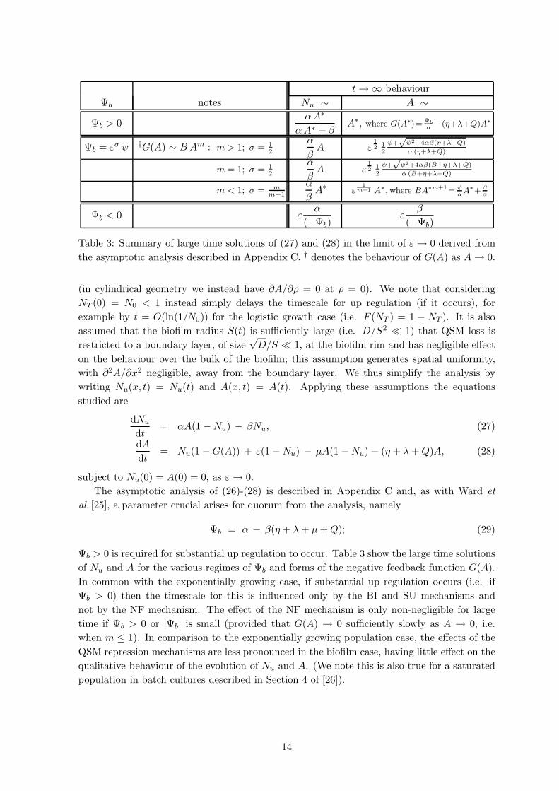
Table 3: Summary of large time solutions of (27) and (28) in the limit of ε→ 0 derived from

the asymptotic analysis described in Appendix C. † denotes the behaviour of G(A) as A→ 0.

(in cylindrical geometry we instead have ∂A/∂ρ = 0 at ρ = 0). We note that considering

NT (0) = N0 < 1 instead simply delays the timescale for up regulation (if it occurs), for

example by t = O(ln(1/N0)) for the logistic growth case (i.e. F (NT ) = 1 − NT ). It is also

assumed that the biofilm radius S(t) is sufficiently large (i.e. D/S2 1) that QSM loss is

restricted to a boundary layer, of size√D/S 1, at the biofilm rim and has negligible effect

on the behaviour over the bulk of the biofilm; this assumption generates spatial uniformity,

with ∂2A/∂x2 negligible, away from the boundary layer. We thus simplify the analysis by

writing Nu(x, t) = Nu(t) and A(x, t) = A(t). Applying these assumptions the equations

studied are

dNu

dt= αA(1 −Nu) − βNu, (27)

dA

dt= Nu(1 −G(A)) + ε(1 −Nu) − µA(1 −Nu) − (η + λ+Q)A, (28)

subject to Nu(0) = A(0) = 0, as ε→ 0.

The asymptotic analysis of (26)-(28) is described in Appendix C and, as with Ward et

al. [25], a parameter crucial arises for quorum from the analysis, namely

Ψb = α − β(η + λ+ µ+Q); (29)

Ψb > 0 is required for substantial up regulation to occur. Table 3 show the large time solutions

of Nu and A for the various regimes of Ψb and forms of the negative feedback function G(A).

In common with the exponentially growing case, if substantial up regulation occurs (i.e. if

Ψb > 0) then the timescale for this is influenced only by the BI and SU mechanisms and

not by the NF mechanism. The effect of the NF mechanism is only non-negligible for large

time if Ψb > 0 or |Ψb| is small (provided that G(A) → 0 sufficiently slowly as A → 0, i.e.

when m ≤ 1). In comparison to the exponentially growing population case, the effects of the

QSM repression mechanisms are less pronounced in the biofilm case, having little effect on the

qualitative behaviour of the evolution of Nu and A. (We note this is also true for a saturated

population in batch cultures described in Section 4 of [26]).

14

3.2.1 Implications of analysis for quorum sensing repression in biofilms

As in Section 2.4.2, the effects of the repression mechanisms on the timescale for up regulation

and on the up-regulated cell fraction are now studied using the dimensional form of the

parameters. Again we assume that substantial up regulation occurs, so that

Ψb(R0, η) =α

ωr2(κu(R0) − β) − β

ωr2

(

η + ωλ+Q

Ks

)

> 0. (30)

where κu(R0) is given by (39). Similarly to Θ(R0, η) in Section 2.4.2, Ψb(R0, η) is monotonic

decreasing in both R0 (since dκu(R0)/dR0 < 0) and η; hence increasing either parameter

will reduce the parameter ranges for possible up regulation. Assuming the biofilm depth has

reached a steady-state, the timescale TB for up regulation is

TB(R0, η) ∼ 1

ω+(R0, η)ln

(

κu(R0)

κd(R0)

)

, (31)

where

ω+(R0, η) = − 1

2rω

(

α+ η + ω(λ+ β) +Q

Ks

)

+1

2rω

(

(

α+ η + ω(λ− β) +Q

Ks

)2

+ 4ωκu(R0)α

)12

. (32)

The fraction of N∗B of up-regulated cells is given by

N∗B(R0, η, g∞) ∼ αA∗

B(R0, η, g∞)

αA∗B(R0, η, g∞) + βωKs

, (33)

where A∗B(R0, η, g∞) satisfies

G(A∗B) +

(Ks(η + ωλ) +Q)

κu(R0)K2sω

A∗B − ωr2

κu(R0)αΨb(R0, η) = 0.

The effects of each of the repression mechanisms are similar to the exponential case discussed

in Section 2.4.1 and can be summarised as follows.

BI mechanism. It can be shown that ∂N∗B/∂R0 < 0 and, by virtue of κd κu, that

∂TB/∂R0 > 0. Hence, increasing the concentration of the QSE inhibitor R0, results in

the expected response of increasing the timescale for up regulation and decreasing the

large time up-regulated cell density. Moreover, the limit R0 → 0 results in TB → 0 and

N∗B → 1 (since A∗

B → ∞) so, regardless of the other repression mechanisms operating, the

absence of QSE inhibition will lead to the run away of QSM production and, ultimately,

up regulation of all cells in the population.

NF mechanism. Negative feedback again does not affect the timescales of up regulation, but

since ∂N∗B/∂g∞ < 0 the up-regulated cell fraction decreases with increasing strength of

the feedback response.

SU mechanism. It can be shown that ∂ω+/∂η < 0 and ∂A∗B/∂η < 0 so that ∂TB/∂η > 0;

hence, as expected, increasing the rate of soaking up of QSMs leads to an increase in

the timescale for up regulation and a reduced steady-state up-regulated cell fraction.

15

3.3 A note on the role of QSM repression on travelling wave behaviour

In Ward et al. [25] it was shown that, in the limit case ε = 0, equations (23)-(25) can exhibit

travelling wave behaviour for large time, whereby a wave front advances from the steady-state

solutions (N∗u , A

∗), given by (71), towards the trivial solution (Nu = A = 0). The analysis

involved translating the equations to a travelling wave co-ordinate z using√Dz = x− P (t),

where P (t) ∼ Ct as t → ∞ is the position of the front, such that Nu → 0 and A → 0

as z → +∞. It was shown that travelling wave solutions can only exist if Ψb > 0, ε = 0

and NT ≡ 1. The wave speed c = C/√D can be determined by applying linearisation of

the equations in the limit z → +∞, with valid solutions existing for all c lying in the range

0 < cmin ≤ c < ∞ (as with Fisher’s equation); however, for general sufficiently rapidly

decaying initial conditions, c = cmin is as usual the observed wave speed. The equivalent

analysis for the current model proceeds in exactly the same way, whereby defining cmin such

that

Ω(cmin) ≡ 4Υ(cmin) − 27Φ(cmin) = 0, (34)

where

Υ(c) =1

3

(

c− β

c

)2

+ β + µ+ η + λ+Q,

Φ(c) =Ψb

c− 2

27

(

c− β

c

)3

− 1

3(β + µ+ η + λ+Q)

(

c− β

c

)

,

implies valid (non-negative) solutions have c ≥ cmin. We note that since the negative feedback

term is nonlinear and that G(0) = 0, this process has no effect on the wave speed so long as

linear selection of cmin pertains. However, by virtue of (71), the cell density and QSM concen-

tration behind the wave front are affected. We note also that by differentiating Ω(cmin(η); η)

with respect to η and noting from [25] that ∂Ω(c)/∂c > 0, it can be shown that ∂cmin/∂η < 0,

i.e. the wave speed decreases with increasing strength of inhibition of QSM production. It can

also been shown, by reverting to dimensional quantities, that (the dimensional) speed cmin

decreases with R0, so repression by the BI mechanism reduces the wave speed.

4 Discussion

In this paper, two existing models have been extended to investigate in detail the role of three

experimentally observed QS repression mechanisms within exponentially growing colonies

and developing biofilms. The mechanisms investigated involve QSE inhibitors (e.g. RsmA

molecules in P. aeruginosa), negative feedback (e.g. RsaL in P. aeruginosa) and constitu-

tively produced QSM soaking up molecules (e.g. TrlR in A. tumefaciens ). Although the

main focus has been on the P. aeruginosa and A. tumefaciens QS systems, it is likely that

there are equivalent QS repression systems in many species of bacteria both Gram positive and

negative, to which the modelling in this paper should also apply. Using curve fitting techniques

we determined estimates of the model parameters, which lead to good fits with experimental

data. Moreover, the model predicts that either NF or SU is sufficient to obtain the experi-

mentally observed saturation of QSM concentration during the exponential growth phase. We

stress that only some of the parameter estimates can be regarded as reliable (namely K, r and

λ, from independent data, and κu, α, and β from time-course QSM concentration data), as

16

these are the dominant parameters governing the evolution of QSM concentration during this

growth phase. Interestingly, the need for non-negligible value for β predicted by the best-fits

with the current model suggests that turnover in the attachment of the QSP-QSM complex

to the lux-box is a significant process in the dynamics of quorum sensing.

The modelling predicts that the repression mechanisms have most impact on bacterial

populations during the exponential phase of growth, most notably on the eventual up-regulated

cell fraction and on the saturation levels of QSM concentration (provided that g∞ > µΘ/α). It

seems that the main advantage to the bacteria of the QS repression processes is the prevention

of a superfluous runaway of QSM production. Moreover, it is of no benefit for the entire

population of cells to be up-regulated when only a fraction needs to be active. It is interesting

that the simulations shown in Figure 4, using the best-fit parameters, predict that only about

10–20% of the population will be up-regulated; from this it can be supposed that nutrient

expenditure by QS is a relatively small proportion of that which would occur in a system

without QSM repression. Such savings on nutrient resources are likely to be significant for

enhancing bacterial survival, particularly in harsher and nutrient-deprived environments. This

rather low percentage is a striking result, contrasting with much of the current intuition

regarding quorate behaviour; it is, however, plausible that under many circumstances such a

proportion of up-regulated cells will suffice to achieve the required degree of virulence, say

The role of the three mechanisms inferred from the analyses can be summarised as follows.

Background Inhibition (BI). The retarding effect of RsmA on P. aeruginosa is demon-

strated in Figure 4A of Pessi et al. [21], whereby the up regulation of QS activity is ini-

tiated significantly earlier in a rsmA− mutant than in the wild-type. Chugani et al. [6]

observed similar results in their experiments comparing wild-type and qscR− strains;

however, the repressive action of qscR is currently uncertain. The analysis in Sections

2.4.2 and 3.2.1 shows that an increasing (decreasing) QSE inhibitor concentration R0

lengthens (shortens) the timescale for up-regulation (in agreement with experimental

work of Pessi et al. [21]) and reduces (increases) the up-regulated cell fraction. In Sec-

tions 2.4.2 and 3.2.1 it was shown that QSE inhibition is a necessary, but not sufficient,

mechanism to prevent run away of QSM production; either the incorporation of NF or

SU mechanism, for example, in the model is required to predict the levelling off of QSM

concentration observed in our experiments. We note that other mathematical models

include a term that describes the “natural” degredation of mRNA-lasI, the effects of

which, mathematically speaking, will be indistinguishable from the BI repression pro-

cess of the current model. The stability of mRNA-lasI is not known, however, and the

fact that P. aeruginosa has evolved one or more mechanisms to regulate mRNA-lasI

(and many other mRNAs) perhaps indicates that their half-life is too long for efficient

QS regulation; this in turn suggests that over the timescales of interest (a few hours)

natural degradation of mRNA-lasI is negligible.

Negative Feedback (NF). Figure 4A of [6] also shows that the QSM concentration even-

tually levels off in the batch culture of a qscR− strain, which is presumably due to the

activation of the negative feedback process and enhanced production of RsaL, demon-

strating that it too has significant effects on QSM production. The modelling suggests

that negative feedback has no influence on the important timescales of QS, but only

on the final QSM concentration and the up-regulated cell fraction attained. This to

be expected as the molecules involved in negative feedback are themselves regulated

17

by QSMs. This is in contrast to the viewpoint of de Kievit et al. [7] that the negative

feedback function of RsaL in P. aeruginosa is to act as a block to up-regulation at low

cell densities; the current modelling suggests that the BI or SU mechanisms are far more

effective in this regard. It would be interesting to repeat the experiments in Section 2.2

using a rsaL− strain of P. aeruginosa. Here, assumming η = 0, the model predicts that

the QSM concentration will continue to rise in proportion to the bacterial density during

the exponential phase of growth, rather than levelling off. If in such an experiment the

QSM concentration were observed to level off then there must be some other, currently

unknown, repression mechanism regulating QSM production in P. aeruginosa, such as

SU mechanism (and not the BI mechanism, for reasons noted above).

Soaking Up of QSMs (SU). The models predict that the QSM soaking-up rate η signifi-

cantly affects both the timescales and large time outcomes. This perhaps is one of the

functions of TrlR in QS of A. tumefaciens [4]. It would also be interesting to adapt the

experimental procedures described in Section 2.2 to compare QSM output of wild type

and trlR− mutants growing in liquid culture. The model predicts that the mutant will,

unless there are other regulatory processes operating, up regulate earlier, with QSM

levels continually rising throughout the exponential growth phase. It is currently un-

known whether this repression mechanism is generic in bacteria, or peculiar to just a few

species. Nevertheless, the assumption of QSM degradation is common in other mathe-

matical models and care is therefore needed when assessing the biological relevance of

the conclusions drawn from these models’ results.

In summary, the modelling suggests that the BI mechanism is necessary to prevent the over-

production of QSMs, but requires further regulatory processes, such as NF and SU mecha-

nisms, to achieve this. Both BI and SU are involved in the speed of up-regulation and NF and

SU are important in restricting QSM output and up-regulated cell fraction. Hence the combi-

nations BI and NF (as with P. aeruginosa) or BI and SU (perhaps relevent for A. tumefaciens)

are sufficient for fine tuning of the timing and extent of up-regulation. The importance and

robustness of the BI mechanism, as predicted by the modelling, suggests that it is likely to be

a employed by many, if not all, quorum sensing bacteria. To our knowledge, such a process

has thus far been identified only in P. aeruginosa, in which two regulator proteins (namely

RsmA and QscR) are known to be involved. It would therefore be worth seeking equivalent

proteins in other bacterial species.

The prediction that the fraction of up-regulated cells may in practice be relatively small

is perhaps contrary to the usual dogma that almost the whole population, particularly in

cultures, becomes quorate. Experimental work involving QS in growing populations has mea-

sured only the global responses and investigations at an individual cell level, to determine

proportions of up-regulated cells, have yet to be undertaken. Experiments to ascertain indi-

vidual responses, say by using a specially constructed reporter strains in which measurements

of individual responses can be made, would be very worthwhile, not only to determine whether

total or partial up-regulation occurs (which may help validate the model), but also to provide

important insights into the behavioural dynamics of a population regulated by QS. Such in-

sights may prove vital in the development of new therapeutic strategies. For example, a drug

targeting “up-regulated” cells may not be effective due to most of the population actually

being “down-regulated” (as seems to be the case in Figure 4).

18

Repression processes in QS are a relatively new area of research and they have thus far been

identified in only a few species of bacteria. Such processes may be regulated directly by QS

(for example the rsaL system in P. aeruginosa) or regulated by any number of other factors

(such as by other independent regulatory processes or by environmental signals). It seems

likely that such regulatory processes are widespread, perhaps ubiquitous, in quorum sensing

bacteria. It is hoped that the mathematical modelling of this paper offers some useful concrete

insights into the potential roles of different repression mechanisms and will stimulate further

experimental investigation, a number of specific suggestions having been outlined above.

Acknowledgements

J.P. Ward gratefully acknowledges support by a Wellcome Trust Training Fellowship in Math-

ematical Biology (Fellowship ref. 054464/2/98) and the other authors the support of the

BBSRC.

References

[1] K. Anguige, J.R. King, J.P. Ward, and P. Williams. Mathematical modelling of therapies

targeted at bacterial quorum sensing. Submitted.

[2] S. Beck von Bodman, D.R. Majerczak, and Coplin D.L. A negative regulator medi-

ates quorum-sensing control of exopolysaccharide productio in Pantoea stewartii subsp.

stewartii. Proc. Nat. Acad. Sci. USA, 95:7687–7692, 1998.

[3] S.P. Brown and R.A. Johnstone. Cooperation in the dark: signalling and collective action

in quorum-sensing bacteria. Proc. R. Soc. Lond. B, 268:1–5, 2001.

[4] Y. Chai, J. Zhu, and S.C. Winans. TrlR, a defective TraR-like protein of Agrobacterium

tumefaciens, blocks TraR function in vitro by forming inactive TrlR:TraR dimers. Mol.

Microbial., 40:414–421, 2001.

[5] D.L. Chopp, M.J. Kirisits, M.R. Parsek, and B. Moran. A mathematical model of quorum

sensing in a bacterial biofilm. J. Indust. Microbiol. Biotach., 29:339–346, 2002.

[6] S.A. Chugani, M. Whiteley, K.M. Lee, D. D’Argenio, C. Manoil, and E.P. Greenberg.

QscR, a modulator of quorum-sensing signal synthesis and virulence in Pseudomonas

aeruginosa. Proc. Nat. Acad. Sci. USA, 98:2752–2757, 2001.

[7] T. De Kievit, P.C. Seed, J. Nezezon, L. Passador, and B.H Iglewski. RsaL, a novel repres-

sor of virulence gene expression in Pseudomonas aeruginosa. J. Bacteriol., 181:2175–2184,

1999.

[8] S.P. Diggle, K. Winzer, A. Lazdunski, P. Williams, and M. Camara. Advancing the quo-

rum in Pseudomonas aeruginosa: MvaT and the regulation of N-acylhomoserine lactone

production and virulence gene expression. J. Bacteriol., 184:2576–2586, 2002.

[9] J.D. Dockery and J.P. Keener. A mathematical model for quorum sensing in Pseudomonas

aeruginosa. Bull. Math. Biol., 63:95–116, 2001.

19

[10] G. Doring. Pseudomonas aeruginosa infection in cystic fibrosis patients. In M. Campa,

M. M. Bendinelli, and H. Friedman, editors, Pseudomonas aeruginosa as an opportunistic

pathogen. Plenum Press, New York, 1993.

[11] A. Eberhard, A.L. Burlingame, C. Eberhard, K.H. Kenyon, and N.J. Oppenheimer. Struc-

tural identification of the autoinducer of Photobacterium fischeri. Biochem., 20:2444–

2449, 1981.

[12] C. Fuqua and E.P. Greenberg. Listening in on bacateria:acyl-homoserine lactone sig-

nalling. Molec. Cell Biol., 3:685–695, 2002.

[13] S. Heeb, K. Heurlier, C. Valverde, M. Camera, D. Haas, and Williams P. Post-

transcriptional regulation in pseudomonas spp. via the Gac/Rsm regulatory network.

In Some editors, editor, Global post-transcriptional regulation. In preparation.

[14] I.A. Holder. Pseudomonas aeruginosa burn infections: pathogenesis and treatment. In

M. Campa, M.M. Bendinelli, and H. Friedman, editors, Pseudomonas aeruginosa as an

opportunistic pathogen. New York: Plenum Press, 1993.

[15] S. James, P. Nilsson, G. James, S Kjelleberg, and T. Fagerstrom. Luminescence control

in the marine bacterium Vibrio fischeri: an analysis of the dynamics of lux regulation. J.

Mol. Biol., 296:1127–1137, 2000.

[16] A.J. Koerber, J.R. King, J.P. Ward, P. Williams, J.M. Croft, and R.E. Sockett. A math-

ematical model of partial-thickness burn-wound infection by Pseudomonas aeruginosa:

quorum sensing and the build-up to invasion. Bull. Math. Biol., 64:239–259, 2002.

[17] V. Koiv and A. Mae. Quorum sensing controls the synthesis of virulence factors by

modulating rsmA gene expression in Erwinia carotovora subsp. carotovora. Mol. Genet.

Genom., 265:287–292, 2001.

[18] P. Nilsson, A. Olofsson, M. Fagerlind, T. Fagerstrom, S. Rice, S. Kjelleberg, and P. Stein-

berg. Kinetics of the ahl regulatory system in a model biofilm system: how many bacteria

constitute a “quorum”. J. Mol. Biol., 309:631–640, 2001.

[19] M.R. Parsek and E.P. Greenberg. Acyl-homoserine lactone quorum sensing in Gram-

negative bacteria: a signalling mechanism involved in associations with higher organisms.

Proc. Nat. Acad. Sci. USA, 97:8789–8793, 2000.

[20] J.P. Pearson, C. van Dalden, and B.H. Iglewski. Active efflux and diffusion are involved

in transport of Pseudomonas aeruginosa cell-to-cell signals. J. Bacteriol., 181:1203–1210,

1999.

[21] G. Pessi, F. Williams, Z. Hindle, K. Heurlier, M.T.G. Holden, M. Camara, D. Haas, and

P. Williams. The global posttranscriptional regulator RsmA modulates production of

virulence determinants and N-acylhomoserine lactones in Pseudomonas aeruginosa. J.

Bacteriol., 183:6676–6683, 2001.

[22] K.R. Piper, B. von Vodman, and S.K. Ferrand. Conjugation factor of Agrobacterium

tumefaciens regulates Ti plasmid transfer by autoinduction. Nature, 362:448–450, 1993.

20

[23] A. Swiderska, A.K. Berndtson, M. Cha, L. Li, G.M.J. Beadoiun III, J. Zhu, and C. Fuqua.

Inhibition of the Agrobacterium tumefaciens TraR quorum sensing regulator. J. Biol.

Chem., 276:52, 2001.

[24] S. Swift, J.P. Throup, P. Williams, G.P.C. Salmond, and G.S.A.B. Stewart. Quorum

sensing: a population density component in the determination of bacterial phenotype.

Trends Biochem. Sci., 21:214–219, 1996.

[25] J.P. Ward, J.R. King, A.J. Koerber, J.M. Croft, R.E. Sockett, and P. Williams. Early

development and quorum sensing in bacterial biofilms. J. Math. Biol., 47:23–55, 2003.

[26] J.P. Ward, J.R. King, A.J. Koerber, P. Williams, J.M. Croft, and R.E. Sockett. Mathe-

matical modelling of quorum sensing in bacteria. IMA J. Math. Appl. Med. Biol., 18:263–

292, 2001.

[27] H. Withers, S. Swift, and P. Williams. Quorum sensing as an integral component of gene

regulatory networks in Gram-negative bacteria. Curr. Opin. Microbiol., 4:186–193, 2001.

Appendix A: detailed examination of QSM production

The purpose of this appendix is to summarise the intracellular biochemistry behind the QSM

production rate constants κu and κd in equation (3). The synthesis of QSMs by Gram-negative

bacteria involves the transcription of certain genes (belonging to the luxI family of genes) that

output an enzyme (QSE) which in turn promotes QSM production by catalysing the reaction

of the two QSM precursor molecules, S-adenosylmethionine (SAM) and an appropriate Acyl-

ACP (acyl carrier protein) [12]. Figure 2 shows a simplified schematic of the biochemistry of

the primary (las) system in P. aeruginosa, which can be summarised by the chemical reaction

LasI (35)

S + C12 −→ a + M ,

where S,C12, a and M are SAM, C12-ACP, 3-oxo-C12-HSL and the waste product 5′-methyl-

thioadenosine, respectively. We note that both SAM and C12-ACP are produced indepen-

dently of quorum sensing. Defining m to be the concentration of mRNA-lasI and L to be the

concentration of the QSE LasI, and assuming that the concentrations of SAM and C12-ACP

are at fixed constant levels S0 and C0, respectively, then using the law of mass action we may

model QSM production by

dm

dt= Mi − krR0m (36)

dL

dt= klm− kqL, (37)

da

dt= kcS0C0L+ kbS0C0, (38)

where R0 is the concentration of the mRNA-lasI degraders, in this case RsmA (but possibly

also representing QscR within a single “generic” inhibitor); Mi is the mRNA-lasI production

rate by down- (i = d) and up- (i = u) regulated cells, kr is the reaction rate of mRNA-lasI

breakdown by RsmA, kq is the natural decay rate for LasI (no bacterially produced agent that

destroys the enzyme has been identified) and kc and kb are the QSM production rates due

21

to the catalysed and background SAM – C12-ACP reactions, respectively. It is assumed that

Md Mu. For the timescales of interest, we can assume that (36) and (37) have attained

quasi-steady states, i.e. m = Mi/krR0 and L = klm/kq = klMi/kqkrR0, which on substitution

into (38) gives

da

dt=

klkcS0C0

kqkrR0Mi + kbS0C0,

from which we can deduce the expressions

κd =klkcS0C0

kqkrR0Md + kbS0C0, κu =

klkcS0C0

kqkrR0Mu + kbS0C0, (39)

for the rate constants κd and κu, with κd κu. The expressions (39) make explicit the

role of QSE inhibitor molecules on QSM production, whereby the κis are approximately in-

versely proportional (assuming the kbS0C0 term to be relatively small) to the QSE inhibitor

concentration R0.

Appendix B: Asymptotic analysis for exponential phase

B.1 Introduction

In this appendix we exploit the fact that ε is small and seek asympotitic solutions to the

system (10) and (11), subject to nu(0) = 0 and a(0) = 0, in the limit ε → 0. We note

that the experimental data suggests there are vast differences between the relative sizes of

the parameters, so further simplifications could also be made. However, sufficient progress

can be achieved without such modifications; indeed, variability across bacteria species and

environmental differences could result in different balances between the parameters, so it

is appropriate to seek solutions for rather general cases. The approach is similar to that

used in the analysis described in Ward et al. [26] and only brief references are made to those

solutions which are eqiuvalent; more detail is given of the new solutions. The analysis of

[26] is also generalised here to consider a general initial cell density nT (0) = N0 1, rather

than N0 = O(ε). As noted in the main text, the most important parameter in governing the

evolution of nu and a is

Θ =α

µ+ η+ γ − β − 2. (40)

In Section B.2 we summarise the analysis for Θ = O(1), expanding on the work described

in [26] to include the QSM repression terms and in Section B.3 we examine more closely the

asymptotic behaviour for |Θ| ∼ 0, which is the borderline parameter regime. We note that all

the analysis to follow applies for the double limit of ε→ 0 and N0 → 0.

B.2 Θ = O(1)

In this section we focus on the case where Θ = O(1) can be of either sign. The important

timescales are considered in turn.

22

B.2.1 t = O(1)

On this timescale the production of QSMs is preformed chiefly by down-regulated cells and

the appropriate rescalings are

t = t, nu = N20 ε n ∼ N2

0 ε n0, a = N0 ε a ∼ N0 ε a0,

leading to a system and solutions equivalent to (12)-(15) in [26], but with N0 = 1. Of note is

the behaviour as t → ∞, which leads to nu = O(εN20 e2t) and a = O(εN0 e

t), so the leading

order balance breaks down when t ∼ ln(1/N0), when nu becomes comparable to a.

B.2.2 t = ln(1/N0) +O(1)

On this timescale nu = O(ε) and a = O(ε) and, again, the analysis of Section 4.3 of [26] applies.

The analysis of this timescale gives rise to the important parameter Θ, which determines

whether a substantial proportion of a population can be up regulated. Writing t = ln(1/N0)+t,

then it can be shown that the leading order solutions for t = O(1) satisfy, when Θ > 0,

nu ∼ εNc eΘ t nT , a ∼ εNc

µ+ ηeΘ t, (41)

as t→ ∞ for some constant Nc, and for Θ < 0 we instead have

nu ∼ εα

(µ+ η)(−Θ)nT , a ∼ ε

α+ (µ+ η)(−Θ)

(µ+ η)2(−Θ), (42)

as t → ∞ with ε 1; we note that the equivalent expression for nu of [26] is erroneous

and should be as given by (42). We observe from (42) that the expressions are singular as

Θ → 0−, the leading order balances changing for sufficiently small Θ; this motivates the

analysis of Section B.3. We observe from (41) that, for Θ > 0, nu is grows faster than nTand for t = ln(1/ε)/Θ + O(1) new balances in the system arise. For Θ < 0 there are no

further timescales of interest and the analysis is complete; we note that a = O(ε) and there

is insufficient QSM accumulation for the negative feedback mechanism to operate at leading

order.

B.2.3 Θ > 0 and t = ln(1/N0) + ln(1/ε)/Θ +O(1)

The relevant scalings for this timescale are

t = ln(1/N0) + ln(1/ε)/Θ + t†, nu = ε−1/θn† ∼ ε−1/θn†0, a = a† ∼ a†0,

which, by matching with (41) as t† → −∞, leads to the leading order system

dn†0dt†

= (γ − 1 − β)n†0 + αa†0(et† − n†0), (43)

n†0 =(µ+ η) a†0e

t†

µa†0 + (1 − g(a†0)), (44)

which combine to give the separable equation

da†0dt†

=1 − g(a†0) + µa†0

(µ+ η)(1 − g(a†0) + a†0g′(a†0))

P (a†0) a†0, (45)

23

where g′(a) = dg/da and

P (a) = (µ+ η)Θ − αη a − αg(a). (46)

Since g(a†0) ≤ g∞ ≤ 1 and g(a†0) → 0 as t† → −∞ the right-hand side of (45) is positive, hence

a†0 is monotonic increasing. Since P (0) = (µ + η)Θ > 0 and P ′(a) = −α(η + g′(a)) < 0, the

large-time behaviour of (45) is dependent on whether there exists a steady-state a†0∗> 0 such

that P (a†0∗) = 0. There are two cases to consider, namely η > 0 (where a†0

∗> 0 always exist)

and η = 0 (where a solution a†0∗> 0 exists only if µΘ/α < g∞).

η > 0. Since P (a) → −∞ as a→ ∞ there exists a unique a†0∗> 0 such that P (a†0

∗) = 0, with

a ∼ a†∗0 = P−1(0), nu ∼ (µ+ η) a†∗0

µa†∗0 + 1 − g(a†∗0 )nT , (47)

as t† → ∞. We note in the absence of the NF mechanism, i.e. g(a) ≡ 0, then a†∗0 =

(µ+ η)Θ/αη.

η = 0. In this case P (a) reduces to P (a) = µΘ − αg(a) and the large-time outcomes are

dependent on whether (i) g∞ > µΘ/α, (ii) g∞ = µΘ/α or (iii) g∞ < µΘ/α.

(i) g∞ > µΘ/α. In this case a†0 tends to a steady-state a†0∗

= g−1(µΘ/α), as t† → ∞and

a ∼ a†0∗, nu ∼ µa†0

∗

µa†0∗

+ 1 − g(a†0∗)nT , (48)

as t† → ∞. The analysis for this case is then complete.

(ii) g∞ = µΘ/α. In this case, the right-hand side of (45) vanishes only when a†0 → ∞and for large a†0 we have

da†0dt†

∼ α

Θg(a†0) a

†0,

as t† → ∞, where g(a) = µΘ/α − g(a), so that g(∞) = 0 and g′(a) < 0. The

evolution of a†0 in large time depends on the behaviour of g(a†0) as a†0 → ∞. However,

since g(a) vanishes as a → ∞ growth of a†0 is sub-exponential; consequently, there

are no further timescales of interest to consider. Using the original variables, the

outcomes for two likely candidates for g(a) as a→ ∞ are

nu ∼ nT , a ∼

(

c α(m + 1)

Θ

)1

m+1

t†1/m+1

g(a) ∼ c

a(m+1),

1

mln(t†) g(a) ∼ c e−m a,

as t† → ∞, where m and c are positive constants.

(iii) g∞ < µΘ/α. Again equation (45) has no steady-states and a†0 will continue to

grow. Assuming, for simplicity, that ag′(a) → 0 as a → ∞, as would be likely for

relevant forms of g(a), we have

da†0dt†

∼ µΘ − αg∞µ(1 − g∞)

(

(1 − g∞)a†0 + µa†02)

, (49)

24

as t† → ∞, a separable equation that solves to give

a†0 ∼ (1 − g∞) eµZt†

(1 − g∞)A0 − µ eµZt†, (50)

where A0 is a positive constant of integration and Z = (µΘ−αg∞)/µ(1− g∞). We

note from (44) that

n†0 ∼ N0 et† , (51)

as t† → ∞. Here the expansions fail when the denominator of (50) becomes zero,

corresponding to t† ∼ t†c(0) = ln((1 − g∞)A0/µ)/µZ, leading to blow up of the

solution a†0. The analysis about the transition period corresponding to the near

blow-up region is a straightforward extension to the analysis described in Sections

4.4.2 and 4.4.3 in [26] and we will omit the details. However, following this transition

period a further rescaling of the form

t = ln(1/N0) + ln(1/ε)/Θ + t‡, nu = ε−1/Θn‡, a = ε−1/Θa‡, (52)

eventually leads to the large time solutions

nu ∼ nT , a ∼ µΘ − αg∞α(1 + λ)

nT , (53)

as t‡ → ∞. We note that a grows exponentially, in contrast to the g∞ > µΘ/α

case, and that the solutions of [26] can be derived by setting g∞ = 0 in (53).

The analysis demonstrates that in order to get saturation of QSM concentration during expo-

nential population growth with small ε, we need either η > 0 or g∞ < µΘ/α, as ε→ 0.

B.3 |Θ| 1

In this section we examine the evolution of nu and a in the vicinity of Θ = 0. It turns out

that the evolution of a and nu in this limit is governed by the behaviour of g(a) as a→ 0. We

shall consider a fairly general case in which

g(a) ∼ B am, (54)

as a→ 0 where B and m are both positive constants. Rather than consider the case of Θ = 0,

as we did in [26], it is more instructive to seek solutions for small Θ and, given (54), the

appropriate scaling for the relevant distinguished limit is

Θ =

εmm+1 θ m < 1,

ε12 θ m ≥ 1,

(55)

the latter case implying no negative feedback. The analysis below starts from the t =

ln(1/N0) +O(1) timescale, where the solution types diverge depending on the sign of Θ.

25

B.3.1 t = ln(1/N0) +O(1)

The appropriate rescalings are

t = ln(1/N0) + t, nu ∼ εn0 + εδ+1n1, a ∼ εa0 + εδ+1a1, (56)

where δ = m/(m + 1) and δ = 1/2 for the m < 1 and m ≥ 1 cases, respectively, which, for

brevity combining the leading- and second-order expressions, leads to

dN

dt= N + αAet − α

µ+ ηN + εδ θn1,

dA

dt= N − (µ+ η)Aet − λA+ et,

where N = n0 + εδn1 and A = a0 + εδa1. Of most interest is the large time behaviour, namely

nu ∼ εN ∼ ε

(

α

µ+ ηt + εδ

1

2

α θ

µ+ ηt 2

)

nT , (57)

a ∼ εA ∼ εα

(µ+ η)2t + εδ+1 1

2

α θ

(µ+ η)2t 2, (58)

as t → ∞. We observe that the correction terms are of the same order as the leading terms

when t = O(ε−δ), marking the onset of a new balance in the system. We note that for Θ = 0

(i.e. θ = 0) and η = 0, the analysis of [26] is recovered and the expansions breakdown when

t = O(1/ε).

B.3.2 t = ln(1/N0) + O(ε−δ)

The appropriate rescalings are

t = ln(1/N0) + ε−δt†, nu ∼ ε1−δ eε−δt†n†0, a ∼ ε1−δa†0,

noting that 1 − δ > 0 in both cases, which, to leading order, yields

n†0 = (µ+ η) a†0,

and

da†0dt†

=

α

(µ+ η)2+ θa†0 − αB

µ+ ηa†0

m+1m < 1,

α

(µ+ η)2+ θa†0 − α (B + η)

µ+ ηa†0

2m = 1,

α

(µ+ η)2+ θ a†0 − αη

µ+ ηa†0

2m > 1,

(59)

subject to a†0(0) = 0 (by matching). For m < 1 the large time behaviour is

a ∼ ε1

m+1 a†0∗, nu ∼ ε

1m+1 (µ+ η) a∗ nT , (60)

as t† → ∞, where the positive constant a†0∗

satisfies p(a†0∗) = 0, where

p(a) = am+1 − θ(µ+ η)

αBa − 1

(µ+ η)B; (61)

26

it is straightforward to show that there is only one such solution for a∗ satisfying p(a∗) = 0.

For m ≥ 1 we have

a ∼ ε12 a†0

∗nu ∼ ε

12 (µ+ η) a†0

∗nT , (62)

as t† → ∞ and ε→ 0, where

a†0∗

=

(η + µ)2 θ +√

θ2(µ+ η)4 + 4α2η(µ+ η)

2αη(µ + η)m > 1

(η + µ)2 θ +√

θ2(µ+ η)4 + 4α2η(B + µ+ η)

2αη(B + µ+ η)m = 1.

(63)

We note that (60)-(63) as θ → +∞ and θ → −∞ matches with (47) and (48) as Θ → 0+

and with (42) as Θ → 0−, respectively.

Appendix C: Asymptotic analysis for fixed depth biofilm

C.1 Introduction

In this appendix we study the system (27) and (28) in the limit ε → 0. The purpose of the

analysis is to investigate the important timescales and what, if any, are the effects of repression

processes on the evolution of Nu and A. An important parameter drawn out by the analysis

below is

Ψb = α − β(η + λ+Q+ µ), (64)

whereby the sign of Ψb governs whether substantial up regulation can occur. Most of the

details of the analysis are covered in the appendix of Ward et al. [25] and are only summarised

here.

C.2 Ψb = O(1)

In this section we seek solutions for the case Ψb = O(1), where Ψb could be of either sign.

C.2.1 t = O(1)

On this timescale the down-regulated population governs the QSM production and Nu = O(ε)

and A = O(ε) are both very small. The feedback term has no leading-order effect on this

timescale and leads to the solutions given in [25], whereby as t→ ∞ we have when Ψb < 0

Nu ∼ εα

(−Ψb), A ∼ ε

β

(−Ψb), (65)

i.e. both tend to constant levels of size O(ε), and when Ψb > 0

Nu ∼ εα(−ω−)

Ψb(ω+ − ω−)eω+t, A ∼ ε

Ψb − βω−

Ψb(ω+ − ω−)eω+t, (66)

where

ω± = − β + µ+ η + λ+Q

2± 1

2

√

(β + µ+ η + λ+Q)2 + 4Ψb; (67)

27

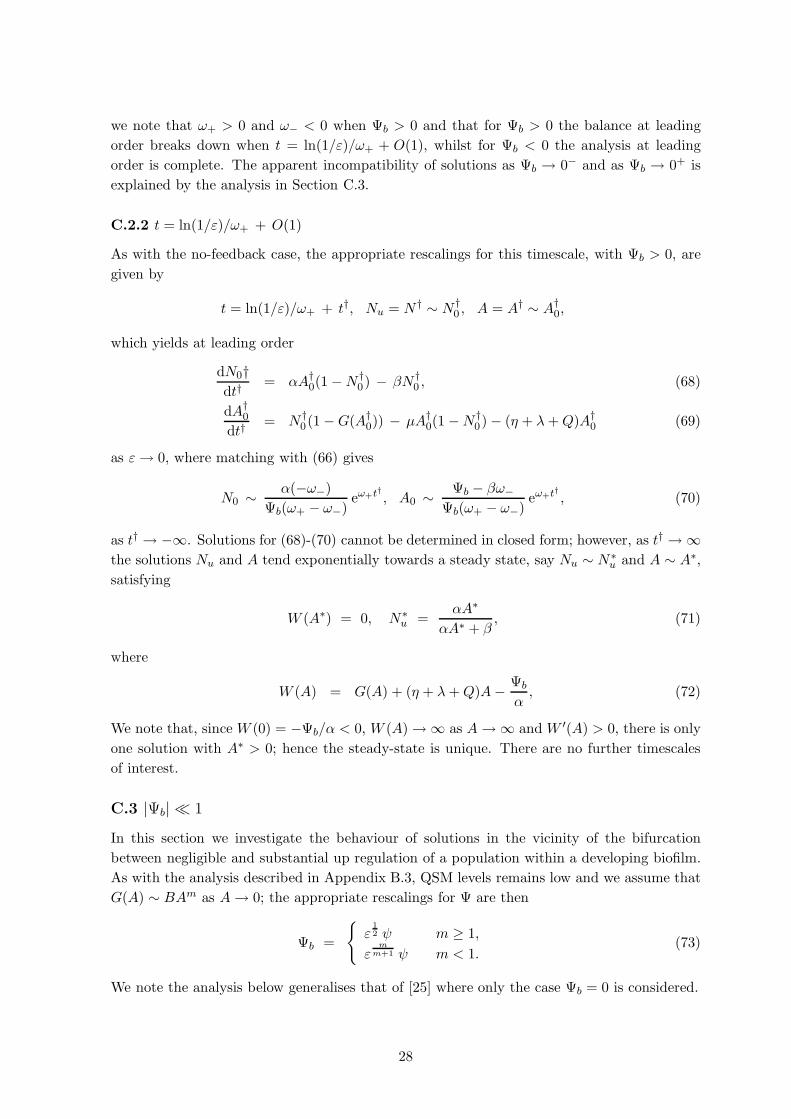
we note that ω+ > 0 and ω− < 0 when Ψb > 0 and that for Ψb > 0 the balance at leading

order breaks down when t = ln(1/ε)/ω+ + O(1), whilst for Ψb < 0 the analysis at leading

order is complete. The apparent incompatibility of solutions as Ψb → 0− and as Ψb → 0+ is

explained by the analysis in Section C.3.

C.2.2 t = ln(1/ε)/ω+ + O(1)

As with the no-feedback case, the appropriate rescalings for this timescale, with Ψb > 0, are

given by

t = ln(1/ε)/ω+ + t†, Nu = N † ∼ N †0 , A = A† ∼ A†

0,

which yields at leading order

dN0†dt†

= αA†0(1 −N †

0) − βN †0 , (68)

dA†0

dt†= N †

0(1 −G(A†0)) − µA†

0(1 −N †0) − (η + λ+Q)A†

0 (69)

as ε→ 0, where matching with (66) gives

N0 ∼ α(−ω−)

Ψb(ω+ − ω−)eω+t† , A0 ∼ Ψb − βω−

Ψb(ω+ − ω−)eω+t† , (70)

as t† → −∞. Solutions for (68)-(70) cannot be determined in closed form; however, as t† → ∞the solutions Nu and A tend exponentially towards a steady state, say Nu ∼ N∗

u and A ∼ A∗,

satisfying

W (A∗) = 0, N∗u =

αA∗

αA∗ + β, (71)

where

W (A) = G(A) + (η + λ+Q)A− Ψb

α, (72)

We note that, since W (0) = −Ψb/α < 0, W (A) → ∞ as A→ ∞ and W ′(A) > 0, there is only

one solution with A∗ > 0; hence the steady-state is unique. There are no further timescales

of interest.

C.3 |Ψb| 1

In this section we investigate the behaviour of solutions in the vicinity of the bifurcation

between negligible and substantial up regulation of a population within a developing biofilm.

As with the analysis described in Appendix B.3, QSM levels remains low and we assume that

G(A) ∼ BAm as A→ 0; the appropriate rescalings for Ψ are then

Ψb =

ε12 ψ m ≥ 1,

εmm+1 ψ m < 1.

(73)

We note the analysis below generalises that of [25] where only the case Ψb = 0 is considered.

28

C.3.1 t = O(1)

The analysis of the [25] is modified using the rescaling (73) to give

A ∼ εβ

β + µ+ η + λ+Qt + εσ+1 1

2

β ψ

(β + µ+ η + λ+Q)2t2, Nu ∼ α

βA, (74)

as t → ∞, where σ = 1/2 and σ = m/(m + 1) for m ≥ 1 and m < 1, respectively. We note

that the leading and correction terms become of the same order (i.e. the expansion disorders)

when t = O(ε1/2) for m ≥ 1 and t = O(εm/m+1) for m < 1, marking the onset of a new

balance in the limit ε→ 0.

C.3.2 Large time

We consider the cases of m ≥ 1 and m < 1 separately.

m ≥ 1. The appropriate rescalings are

t = t†/ε1/2, Nu = ε1/2N † ∼ ε1/2N †0 , A = ε1/2A† ∼ ε1/2A†

0,

from which we can deduce

N †0 =

α

βA†

0, (75)

dA†0

dt=

1

β + µ+ η + λ+Q

(

β + ψA†0 − αA†

0

2(η + λ+Q) − εm−1BA†

0

m+1)

, (76)

as ε → 0, subject to A†0(0) = 0 (by matching with (74)). We note that the feedback

response term in equation (76) (i.e. he B term) does not of course appear in these

leading-order euations when m > 1. For both cases m = 1 and m > 1, equation (76)

can be integrated explicitly, and as t→ ∞ we have the steady-states

A ∼√ε

1

2

ψ +√

ψ2 + 4αβ (η + λ+Q)

α (η + λ+Q)m > 1,

1

2

ψ +√

ψ2 + 4αβ (B + η + λ+Q)

α (B + η + λ+Q)m = 1,

(77)

and Nu ∼ αA/β from (75).

m < 1. The appropriate rescalings are

t = ε−mm+1 t†, Nu = ε

1m+1N † ∼ ε

1m+1N †

0 , A = ε1

m+1A† ∼ ε1

m+1A†0,

leading to (75) and

dA†0

dt=

1

β + µ+ η + λ+Q

(

β + ψA†0 − αB A†

0

m+1)

, (78)

subject to A†0(0) = 0. Hence A evolves to a steady state A ∼ ε1/(m+1)A∗ as t→ ∞, with

A∗ satisfying q(A∗) = 0, where

q(A) = Am+1 − ψ

αBA − β

αB; (79)

it is straightforward to show that there is only one positive solution A∗ satisfying q(A∗) =

0. From (75) we have Nu ∼ αA∗/β as t→ ∞.

We note that these steady-states can be shown to match as ψ → +∞ with (71) for Ψb → 0+

and as ψ → −∞ with (65) for Ψb → 0−.

29

List of Figures

1 Schematic of the feedback process of the primary QS system in Pseudomonas

aeruginosa. The italics within the large arrows represent the genes producing

LasR (the QSP), 3-oxo-C12-HSL (the QSM) and the negative feedback protein

RsaL. Vfr and GacA are two external regulators known to be involved in the

production of LasR, and RsmA, while QscR is believed to be external repressors

of QSM production. The solid curves (labelled with a (+)) and dashed curves

(labelled with a (-)) are the positive and negative influences, respectively, on

the system. . . . . . . . . . . . . . . . . . . . . . . . . . . . . . . . . . . . . . . 31

2 Schematic of the transcription of the lasI gene in the production of QSM 3-oxo-

C12-HSL. The gene encodes the QSE LasI, which catalyses the reaction between

SAM (S-adenosylmethionine) and C12-ACP to produce the QSM and the waste

product MTA (5′-methylthioadenosine). RsmA is a global translational regu-

lator protein which destroys messenger RNA including that transcripted from

the lasI gene. . . . . . . . . . . . . . . . . . . . . . . . . . . . . . . . . . . . . . 32

3 Plot of QSM concentration against time, comparing model solutions using best-

fit parameters for BI-NF (g∞ > 0, η = 0, solid curve), BI-SU (g∞ = 0, η > 0,

dashed curve) and BI only (g∞ = 0, η = 0, dotted curve) cases with experi-

mental data for QSM production in LB (indicated by the • s). The BI only

case cannot predict saturation of QSM concentration and the curve shown is

the best fit with data up t = 4 hours. We note that the quantities involved are

dimensional. . . . . . . . . . . . . . . . . . . . . . . . . . . . . . . . . . . . . . . 32

4 Predicted evolution of the up-regulated cell fraction using the best-fit param-

eters listed in Table 1 for BI-NF (solid curve), BI-SU (dashed curve) and BI

only (dotted curve) cases. . . . . . . . . . . . . . . . . . . . . . . . . . . . . . . 33

5 Plot of the evolution of the population density (solid curves) and drug con-

centration (dashed curves) in response to initial drug dosages of w0 = 16 and

w0 = 17, with δ = 10. The other dimensionless parameter values are determined

from the data given in the first column in Table 1. . . . . . . . . . . . . . . . . 33

6 Plot of the bifurcation curves in δ–w0 space for various values of g∞. Parameter

regimes above each curve result ultimately result in an exponential decline of the

population, below each curve the population will ultimately grow exponentially.

The other dimensionless parameter values are determined from the data given

in the first column in Table 1. . . . . . . . . . . . . . . . . . . . . . . . . . . . 34

30

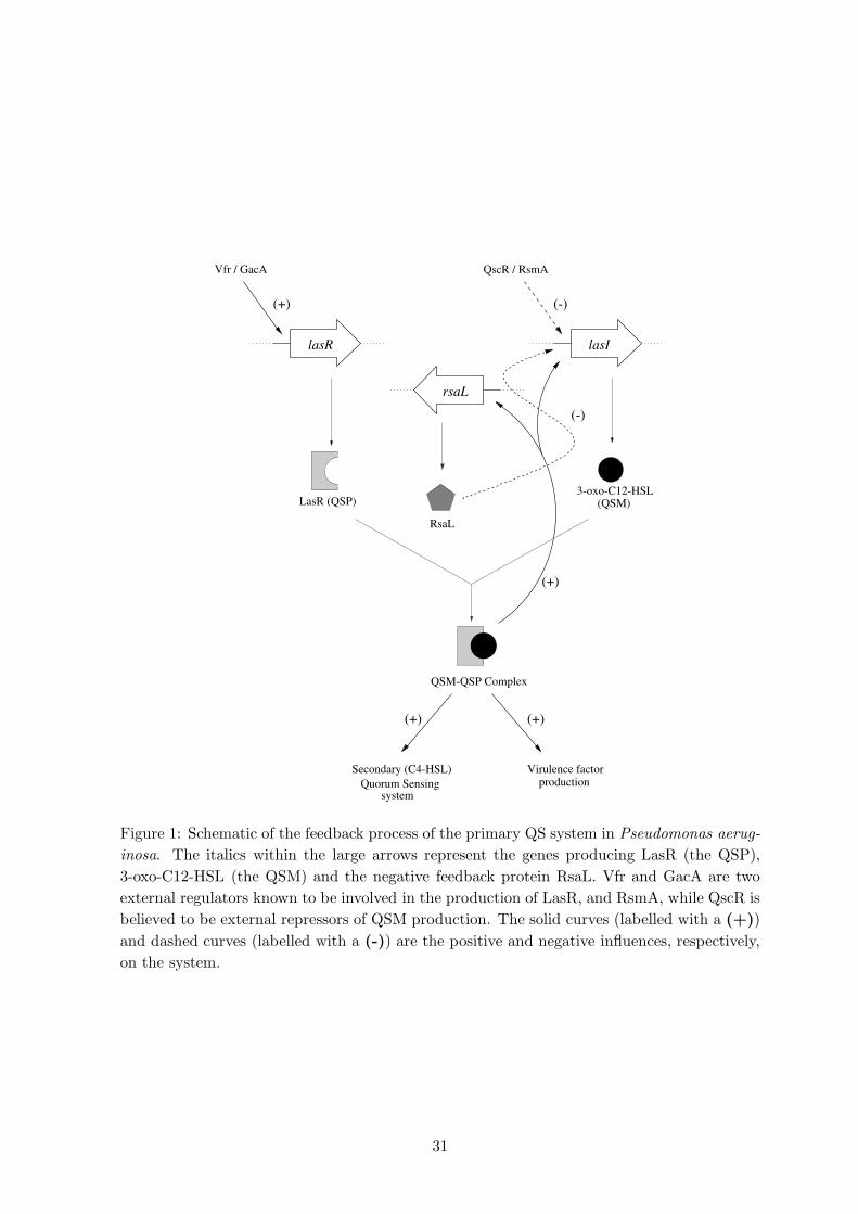
Secondary (C4-HSL)

Quorum Sensingsystem

(+)

Virulence factor production

(+)

QSM-QSP Complex

Vfr / GacA

(+)

lasR lasI

LasR (QSP)3-oxo-C12-HSL

(QSM)

RsaL

rsaL

(-)

(+)

QscR / RsmA

(-)

Figure 1: Schematic of the feedback process of the primary QS system in Pseudomonas aerug-

inosa. The italics within the large arrows represent the genes producing LasR (the QSP),

3-oxo-C12-HSL (the QSM) and the negative feedback protein RsaL. Vfr and GacA are two

external regulators known to be involved in the production of LasR, and RsmA, while QscR is

believed to be external repressors of QSM production. The solid curves (labelled with a (+))

and dashed curves (labelled with a (-)) are the positive and negative influences, respectively,

on the system.

31

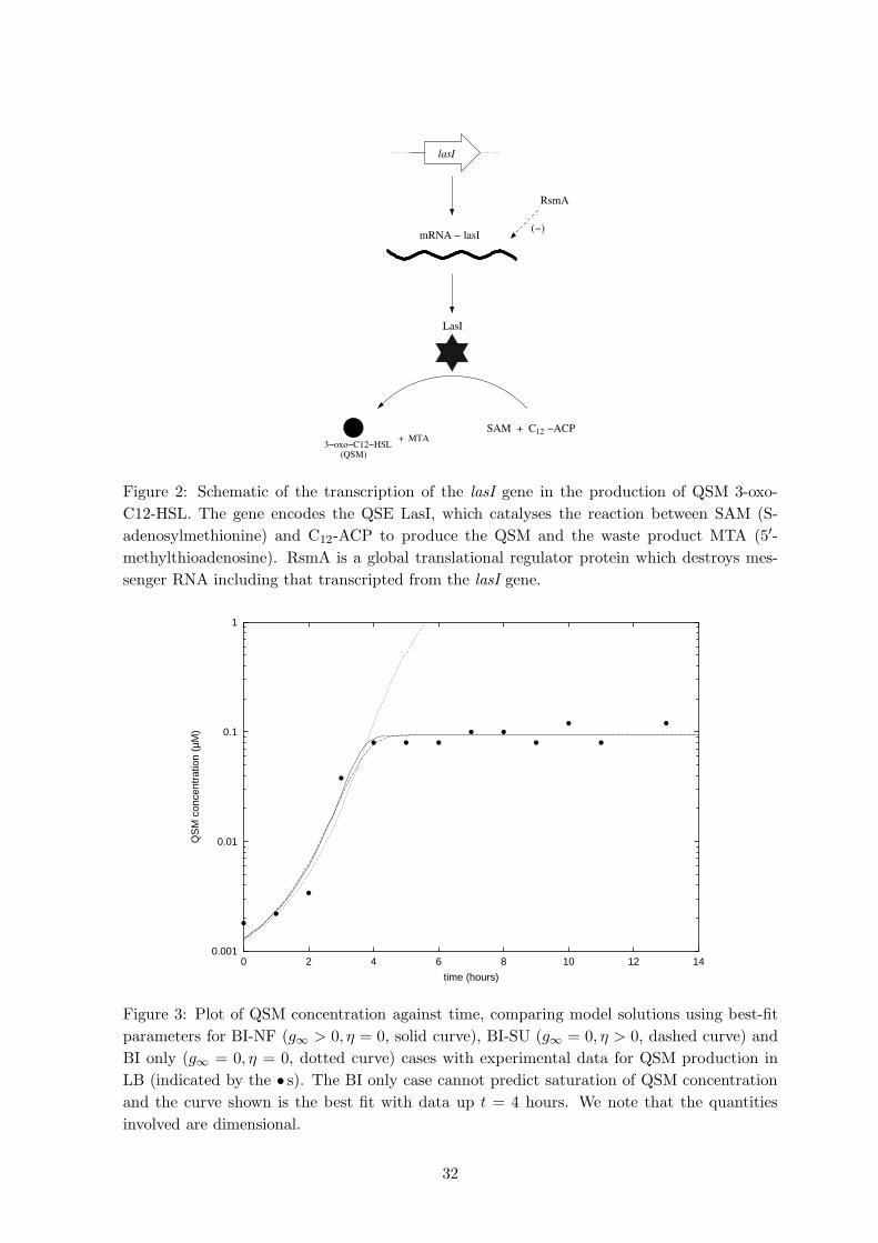
mRNA − lasI

lasI

3−oxo−C12−HSL(QSM)

+ MTASAM + C −ACP12

LasI

(−)

RsmA

Figure 2: Schematic of the transcription of the lasI gene in the production of QSM 3-oxo-

C12-HSL. The gene encodes the QSE LasI, which catalyses the reaction between SAM (S-

adenosylmethionine) and C12-ACP to produce the QSM and the waste product MTA (5′-

methylthioadenosine). RsmA is a global translational regulator protein which destroys mes-

senger RNA including that transcripted from the lasI gene.

0.001

0.01

0.1

1

0 2 4 6 8 10 12 14

QS

M c

once

ntra

tion

(µM

)

time (hours)

Figure 3: Plot of QSM concentration against time, comparing model solutions using best-fit

parameters for BI-NF (g∞ > 0, η = 0, solid curve), BI-SU (g∞ = 0, η > 0, dashed curve) and

BI only (g∞ = 0, η = 0, dotted curve) cases with experimental data for QSM production in

LB (indicated by the • s). The BI only case cannot predict saturation of QSM concentration

and the curve shown is the best fit with data up t = 4 hours. We note that the quantities

involved are dimensional.

32

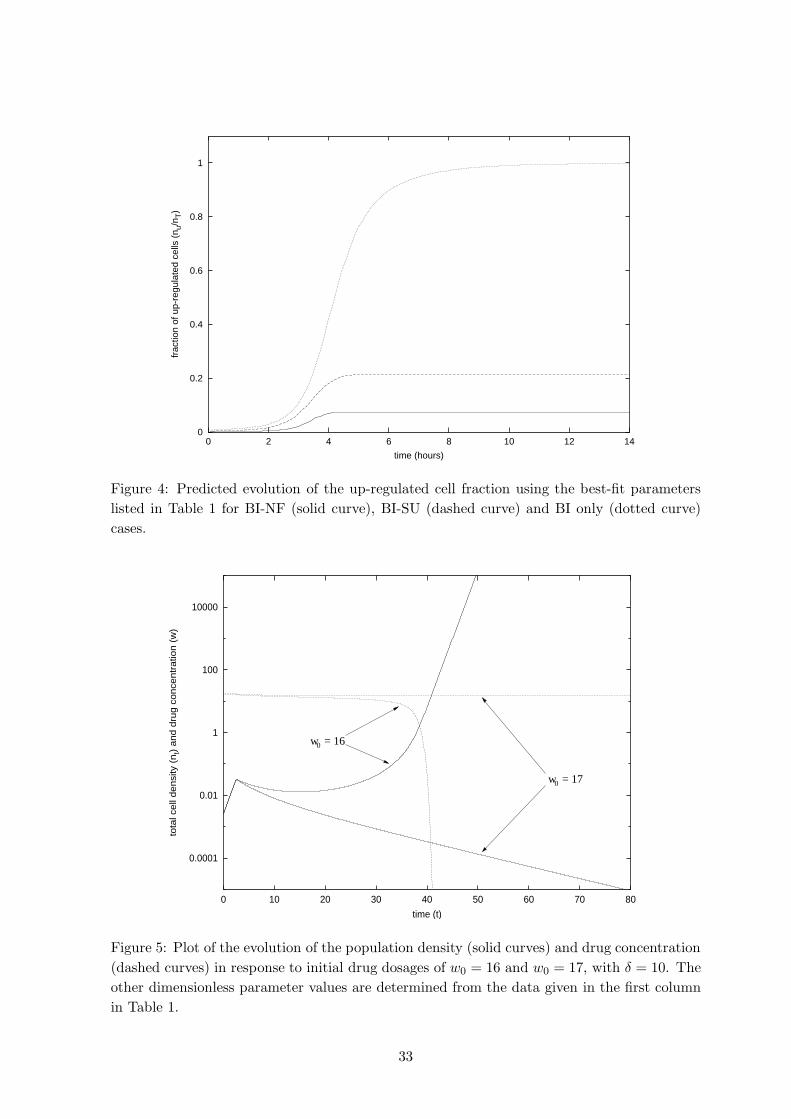
0

0.2

0.4

0.6

0.8

1

0 2 4 6 8 10 12 14

frac

tion

of u

p-re

gula

ted

cells

(n u

/nT)

time (hours)

Figure 4: Predicted evolution of the up-regulated cell fraction using the best-fit parameters

listed in Table 1 for BI-NF (solid curve), BI-SU (dashed curve) and BI only (dotted curve)

cases.

0.0001

0.01

1

100

10000

0 10 20 30 40 50 60 70 80

tota

l cell

densi

ty (

nt) a

nd d

rug c

once

ntr

atio

n (

w)

time (t)

0

w = 170

w = 16

Figure 5: Plot of the evolution of the population density (solid curves) and drug concentration

(dashed curves) in response to initial drug dosages of w0 = 16 and w0 = 17, with δ = 10. The

other dimensionless parameter values are determined from the data given in the first column

in Table 1.

33

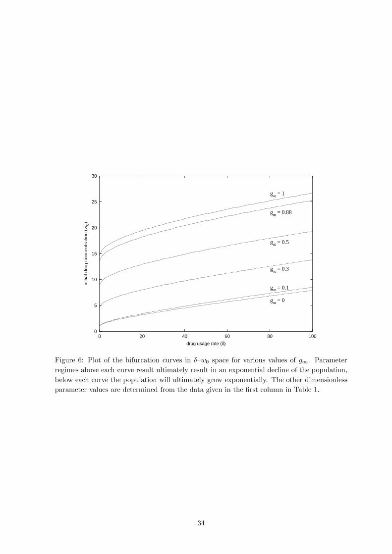
0

5

10

15

20

25

30

0 20 40 60 80 100

initi

al d

rug c

once

ntr

atio

n (

w0)

drug usage rate (δ)

g = 1

g = 0.88

g = 0.5

g = 0.3

g = 0.1

g = 0

88

88

88

Figure 6: Plot of the bifurcation curves in δ–w0 space for various values of g∞. Parameter

regimes above each curve result ultimately result in an exponential decline of the population,

below each curve the population will ultimately grow exponentially. The other dimensionless

parameter values are determined from the data given in the first column in Table 1.

34