CED 2014-2024 Revised Forecast Volume 1 - California ... ENERGY DEMAND 2014–2024 REVISED FORECAST...

CALIFORNIA ENERGY DEMAND

2014–2024 REVISED FORECAST

Volume 1: Statewide Electricity Demand, End‐User Natural Gas Demand, and Energy Efficiency

SEPTEMBER 2013

CEC ‐200 ‐2013 ‐004 ‐SD ‐V1 ‐REV

CALIFORNIA ENERGY COMMISSION

Edmund G. Brown Jr., Governor

California Energy Commission

DRAFT STAFF REPORT

CALIFORNIA ENERGY COMMISSION Bryan Alcorn Mark Ciminelli Nicholas Fugate Asish Gautam Chris Kavalec Kate Sullivan Malachi Weng-Gutierrez Contributing Authors Chris Kavalec Project Manager Andrea Gough Acting Manager DEMAND ANALYSIS OFFICE Sylvia Bender Deputy Director ELECTRICITY SUPPLY ANALYSIS DIVISION Robert P. Oglesby Executive Director

DISCLAIMER Staff members of the California Energy Commission prepared this report. As such, it does not necessarily represent the views of the Energy Commission, its employees, or the State of California. The Energy Commission, the State of California, its employees, contractors and subcontractors make no warrant, express or implied, and assume no legal liability for the information in this report; nor does any party represent that the uses of this information will not infringe upon privately owned rights. This report has not been approved or disapproved by the Energy Commission nor has the Commission passed upon the accuracy or adequacy of the information in this report.

i

ACKNOWLEDGEMENTS

The demand forecast is the combined product of the hard work and expertise of numerous staff members in the Demand Analysis Office. In addition to the contributing authors listed previously, Mohsen Abrishami prepared the commercial sector forecast. Mehrzad Soltani Nia helped prepare the industrial forecast. Ted Dang ran the Summary Model. Cary Garcia prepared the weather data. Andrea Gough supervised data preparation. Steven Mac and Keith O’Brien prepared the historical energy consumption data. Nahid Movassagh forecasted consumption for the agriculture and water pumping sectors. Cynthia Rogers and Doug Kemmer developed the energy efficiency program estimates. Margaret Sheridan provided estimates for demand response program impacts and contributed to the residential forecast. Mitch Tian prepared the peak demand forecast. Ravinderpal Vaid provided the projections of commercial floor space and number of households.

iii

ABSTRACT

The California Energy Demand 2014 – 2024 Revised Forecast, Volume 1: Statewide Electricity Demand and Methods, End‐User Natural Gas Demand, and Energy Efficiency describes the California Energy Commission’s revised baseline forecasts for 2014 – 2024 electricity consumption, peak, and natural gas demand for each of five major electricity planning areas and three natural gas distribution areas and for the state as a whole. This forecast supports the analysis and recommendations of the 2012 Integrated Energy Policy Report Update and the 2013 Integrated Energy Policy Report. The forecast includes three scenarios: a high energy demand case, a low energy demand case, and a mid energy demand case. The high energy demand case incorporates relatively high economic/demographic growth, relatively low electricity and natural gas rates, and relatively low efficiency program and self‐generation impacts. The low energy demand case includes lower economic/demographic growth, higher assumed rates, and higher efficiency program and self‐generation impacts. The mid case uses input assumptions at levels between the high and low cases. Forecasts are provided at both the planning area and climate zone level.

Keywords: Electricity, demand, consumption, forecast, weather normalization, peak, natural gas, self‐generation, conservation, energy efficiency, climate zone, forecast methods

Please use the following citation for this report:

Kavalec, Chris, Nicholas Fugate, Bryan Alcorn, Mark Ciminelli, Asish Gautam, Kate Sullivan, and Malachi Weng‐Gutierrez. 2013. California Energy Demand 2014‐2024 Revised Forecast, Volume 1: Statewide Electricity Demand, End‐User Natural Gas Demand, and Energy Efficiency. California Energy Commission, Electricity Supply Analysis Division. Publication Number: CEC‐200‐2013‐004‐SD‐V1‐REV.

iv

TABLE OF CONTENTS Page

Acknowledgements ............................................................................................................................. i

Abstract ............................................................................................................................................... iii

Executive Summary ............................................................................................................................ 1

Introduction .......................................................................................................................................... 1

Baseline Electricity Forecast Results ................................................................................................. 1

Baseline Natural Gas Forecast Results ............................................................................................. 4

Conservation/Efficiency ...................................................................................................................... 5

Summary of Changes to Forecast ...................................................................................................... 6

CHAPTER 1: Statewide Baseline Forecast Results and Methods ............................................. 9

Introduction .......................................................................................................................................... 9

Summary of Changes to Forecast .................................................................................................... 10

Changes From Preliminary to Revised Forecast ................................................................... 11

Statewide Baseline Forecast Results ............................................................................................... 12

Annual Electricity Consumption ............................................................................................. 15

Statewide Baseline Peak Demand ........................................................................................... 19

Baseline Natural Gas Demand Forecast ................................................................................. 23

Overview of Methods and Assumptions ....................................................................................... 24

Economic and Demographic Assumptions ........................................................................... 27

Electricity and Natural Gas Rate Projections ......................................................................... 34

Conservation/Efficiency Impacts ............................................................................................. 37

Demand Response ..................................................................................................................... 38

Self‐Generation .......................................................................................................................... 40

Electric Light‐Duty Vehicles .................................................................................................... 44

Additional Electrification ......................................................................................................... 46

Natural Gas Light‐Duty Vehicles ............................................................................................ 48

Subregional Electricity Analysis .............................................................................................. 49

v

Historical Electricity Consumption Estimates ....................................................................... 49

Structure of Report ............................................................................................................................ 50

CHAPTER 2: End‐User Natural Gas Demand Forecast ............................................................. 53

Statewide Baseline Forecast Results ............................................................................................... 53

Planning Area Baseline Results ....................................................................................................... 57

Pacific Gas and Electric Planning Area .................................................................................. 57

Southern California Gas Company Planning Area ............................................................... 61

San Diego Gas & Electric Planning Area ................................................................................ 65

CHAPTER 3: Energy Efficiency and Conservation .................................................................... 70

Introduction ........................................................................................................................................ 70

Committed Energy Efficiency .......................................................................................................... 70

Committed Efficiency Programs ............................................................................................. 75

Price Effects ................................................................................................................................ 78

Building Codes and Appliance Standards ............................................................................. 78

Incremental Achievable Efficiency Savings ................................................................................... 81

List of Acronyms ............................................................................................................................... 83

APPENDIX A: Additional Methodology Documentation and Econometric Results ........ A‐1

Industrial Model .............................................................................................................................. A‐1

Comparison of CED 2013 Revised and Full Econometric Forecasts .......................................... A‐2

Impacts From Climate Change ...................................................................................................... A‐4

Price Elasticities ............................................................................................................................... A‐8

APPENDIX B: Self‐Generation Forecasts .................................................................................. B‐1

Compiling Historical Distributed Generation Data ................................................................... B‐1

Residential Sector Predictive Model ............................................................................................. B‐6

Self‐Generation Forecast, Nonresidential Sectors ....................................................................... B‐9

Commercial CHP and PV Forecast ....................................................................................... B‐9

Other Sector Self‐Generation ................................................................................................... 13

APPENDIX C: Regression Results .............................................................................................. C‐1

vi

LIST OF FIGURES Page

Figure ES‐1: Statewide Baseline Annual Electricity Consumption .............................................. 3

Figure ES‐2: Statewide Baseline Annual Noncoincident Peak Demand ..................................... 4

Figure ES‐3: Total Statewide Committed Efficiency and Conservation Impacts ....................... 6

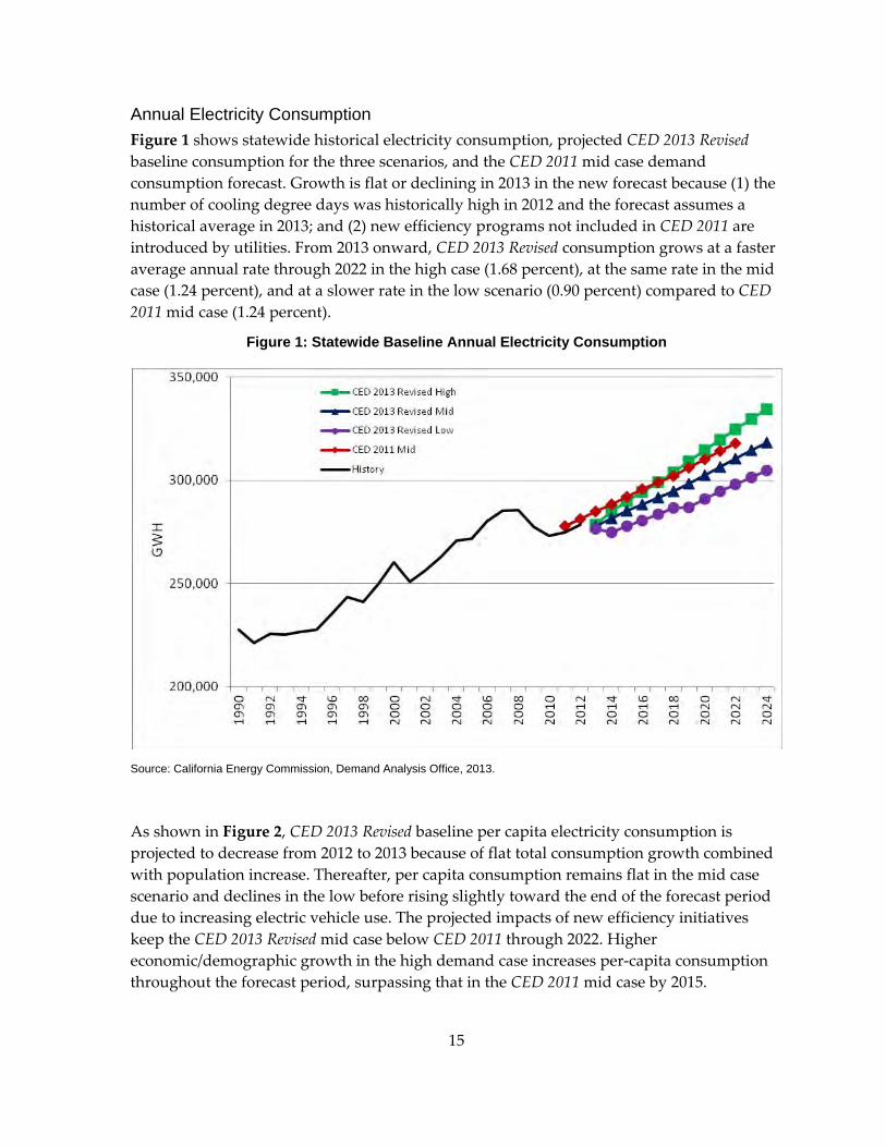
Figure 1: Statewide Baseline Annual Electricity Consumption .................................................. 15

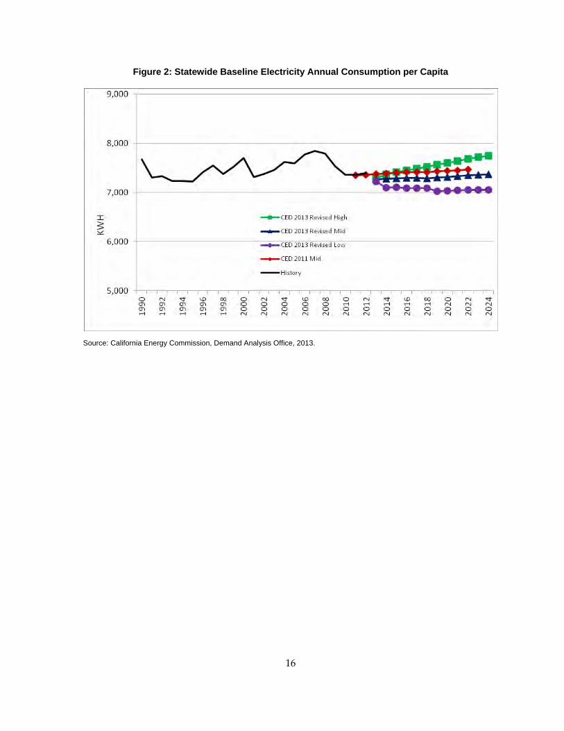
Figure 2: Statewide Baseline Electricity Annual Consumption per Capita ............................... 16

Figure 3: Statewide Baseline Annual Noncoincident Peak Demand ......................................... 20

Figure 4: Statewide Baseline Noncoincident Peak Load Factors ................................................ 21

Figure 5: Statewide Baseline Noncoincident Peak Demand per Capita .................................... 22

Figure 6: Statewide Employment Projections ................................................................................ 30

Figure 7: Statewide Personal Income Projections ......................................................................... 31

Figure 8: Statewide Number of Households Projections ............................................................. 32

Figure 9: Historical and Projected Statewide Population ............................................................ 33

Figure 10: Statewide Projected Commercial Floor Space ............................................................. 34

Figure 11: Total Statewide Committed Efficiency and Conservation Impacts ......................... 38

Figure 12: Statewide Peak Impacts of Self‐Generation ................................................................ 42

Figure 13: Statewide Peak Impacts of PV Systems ....................................................................... 42

Figure 14: Statewide Electric Vehicle Consumption ..................................................................... 45

Figure 15: Statewide Electric Vehicle Peak Demand .................................................................... 46

Figure 16: Energy Commission Forecasting Climate Zones ........................................................ 52

Figure 17: Statewide Baseline End‐User Natural Gas Consumption ......................................... 55

Figure 18: Statewide End‐User Baseline Per Capita Natural Gas Consumption ..................... 56

Figure 19: Statewide Natural Gas Committed Efficiency Impacts ............................................. 57

Figure 20: PG&E Planning Area Baseline Residential Natural Gas Consumption .................. 59

Figure 21: PG&E Planning Area Baseline Commercial Natural Gas Consumption ................ 60

Figure 22: PG&E Planning Area Baseline Industrial Natural Gas Consumption .................... 60

Figure 23: PG&E Planning Area Natural Gas Committed Efficiency Impacts ......................... 61

vii

Figure 24: SoCal Gas Planning Area Baseline Residential Natural Gas Consumption ........... 63

Figure 25: SoCal Gas Planning Area Baseline Commercial Natural Gas Consumption ......... 64

Figure 26: SoCal Gas Planning Area Baseline Industrial Natural Gas Consumption ............. 64

Figure 27: SoCal Gas Planning Area Natural Gas Committed Efficiency Impacts .................. 65

Figure 28: SDG&E Planning Area Baseline Residential Natural Gas Consumption ............... 67

Figure 29: SDG&E Planning Area Baseline Commercial Natural Gas Consumption ............. 68

Figure 30: SDG&E Planning Area Baseline Industrial Natural Gas Consumption .................. 68

Figure 31: SDG&E Planning Area Natural Gas Committed Efficiency Impacts ...................... 69

Figure 32: Historical and Projected Statewide Committed Efficiency Electricity Consumption Savings Impacts ..................................................................................................... 71

Figure 33: Historical and Projected Statewide Committed Electricity Efficiency Peak Savings Impacts .............................................................................................................................. 72

Figure 34: Statewide Natural Gas Committed Efficiency Impacts ............................................. 74

Figure 35: Projected Electricity Savings, 2013 – 2014 IOU Programs, Mid Demand Case ...... 76

Figure 36: Projected Natural Gas Savings, 2013 – 2014 IOU Programs, Mid Demand Case .. 77

Figure 37: Projected Electricity Savings From 2013 POU Programs, Mid Demand Case ....... 78

Figure B‐1: Statewide Historical Distribution of Self‐Generation, All Customer Sectors ..... B‐4

Figure B‐2: Statewide PV Self‐Generation by Customer Sector ................................................ B‐4

Figure B‐3: Median PV Installation Costs and Subsidies, Statewide ....................................... B‐5

Figure B‐4: Statewide Historical Distribution of Self‐Generation, Nonresidential Sectors .. B‐6

Figure B‐5: Distribution of Annual End‐Use Consumption by Fuel Type – North Coastal Small/Medium Buildings .............................................................................................................. B‐10

Figure B‐6: Hourly* Electricity Demand for Large Schools, South Coastal Climate Zones ............................................................................................................................................ B‐10

Figure B‐7: Distribution of Non‐Residential Historical and Modeled PV System Sizes ..... B‐12

Figure B‐8: Residential Sector PV Peak Impact, Statewide ...................................................... B‐14

Figure B‐9: Commercial Sector PV Peak Impact, Statewide .................................................... B‐15

Figure B‐10: Commercial Sector CHP Energy Impact, Statewide .......................................... B‐16

viii

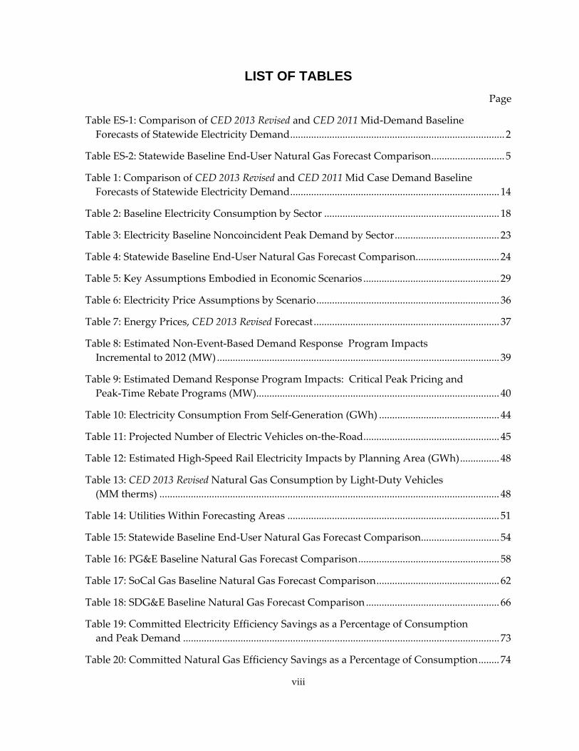
LIST OF TABLES Page

Table ES‐1: Comparison of CED 2013 Revised and CED 2011 Mid‐Demand Baseline Forecasts of Statewide Electricity Demand .................................................................................. 2

Table ES‐2: Statewide Baseline End‐User Natural Gas Forecast Comparison ............................ 5

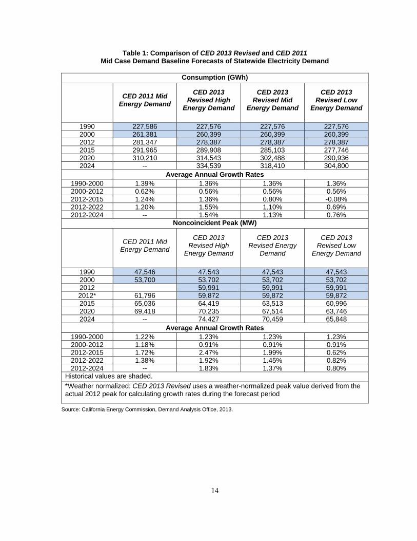
Table 1: Comparison of CED 2013 Revised and CED 2011 Mid Case Demand Baseline Forecasts of Statewide Electricity Demand ................................................................................ 14

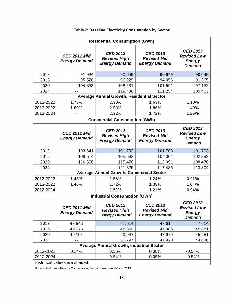
Table 2: Baseline Electricity Consumption by Sector ................................................................... 18

Table 3: Electricity Baseline Noncoincident Peak Demand by Sector ........................................ 23

Table 4: Statewide Baseline End‐User Natural Gas Forecast Comparison ................................ 24

Table 5: Key Assumptions Embodied in Economic Scenarios .................................................... 29

Table 6: Electricity Price Assumptions by Scenario ...................................................................... 36

Table 7: Energy Prices, CED 2013 Revised Forecast ....................................................................... 37

Table 8: Estimated Non‐Event‐Based Demand Response Program Impacts Incremental to 2012 (MW) ............................................................................................................ 39

Table 9: Estimated Demand Response Program Impacts: Critical Peak Pricing and Peak‐Time Rebate Programs (MW)............................................................................................. 40

Table 10: Electricity Consumption From Self‐Generation (GWh) .............................................. 44

Table 11: Projected Number of Electric Vehicles on‐the‐Road .................................................... 45

Table 12: Estimated High‐Speed Rail Electricity Impacts by Planning Area (GWh) ............... 48

Table 13: CED 2013 Revised Natural Gas Consumption by Light‐Duty Vehicles (MM therms) .................................................................................................................................. 48

Table 14: Utilities Within Forecasting Areas ................................................................................. 51

Table 15: Statewide Baseline End‐User Natural Gas Forecast Comparison .............................. 54

Table 16: PG&E Baseline Natural Gas Forecast Comparison ...................................................... 58

Table 17: SoCal Gas Baseline Natural Gas Forecast Comparison ............................................... 62

Table 18: SDG&E Baseline Natural Gas Forecast Comparison ................................................... 66

Table 19: Committed Electricity Efficiency Savings as a Percentage of Consumption and Peak Demand ......................................................................................................................... 73

Table 20: Committed Natural Gas Efficiency Savings as a Percentage of Consumption ........ 74

ix

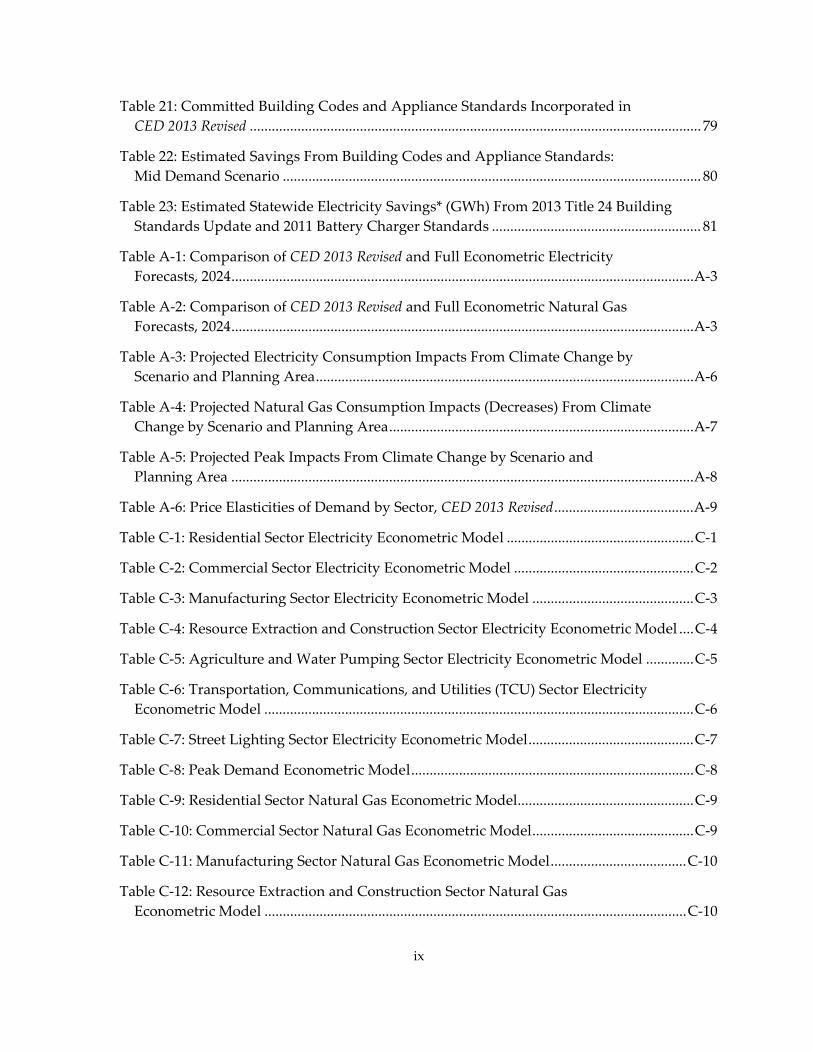
Table 21: Committed Building Codes and Appliance Standards Incorporated in CED 2013 Revised ........................................................................................................................... 79

Table 22: Estimated Savings From Building Codes and Appliance Standards: Mid Demand Scenario .................................................................................................................. 80

Table 23: Estimated Statewide Electricity Savings* (GWh) From 2013 Title 24 Building Standards Update and 2011 Battery Charger Standards ......................................................... 81

Table A‐1: Comparison of CED 2013 Revised and Full Econometric Electricity Forecasts, 2024 .............................................................................................................................. A‐3

Table A‐2: Comparison of CED 2013 Revised and Full Econometric Natural Gas Forecasts, 2024 .............................................................................................................................. A‐3

Table A‐3: Projected Electricity Consumption Impacts From Climate Change by Scenario and Planning Area ....................................................................................................... A‐6

Table A‐4: Projected Natural Gas Consumption Impacts (Decreases) From Climate Change by Scenario and Planning Area ................................................................................... A‐7

Table A‐5: Projected Peak Impacts From Climate Change by Scenario and Planning Area .............................................................................................................................. A‐8

Table A‐6: Price Elasticities of Demand by Sector, CED 2013 Revised ...................................... A‐9

Table C‐1: Residential Sector Electricity Econometric Model ................................................... C‐1

Table C‐2: Commercial Sector Electricity Econometric Model ................................................. C‐2

Table C‐3: Manufacturing Sector Electricity Econometric Model ............................................ C‐3

Table C‐4: Resource Extraction and Construction Sector Electricity Econometric Model .... C‐4

Table C‐5: Agriculture and Water Pumping Sector Electricity Econometric Model ............. C‐5

Table C‐6: Transportation, Communications, and Utilities (TCU) Sector Electricity Econometric Model ..................................................................................................................... C‐6

Table C‐7: Street Lighting Sector Electricity Econometric Model ............................................. C‐7

Table C‐8: Peak Demand Econometric Model ............................................................................. C‐8

Table C‐9: Residential Sector Natural Gas Econometric Model ................................................ C‐9

Table C‐10: Commercial Sector Natural Gas Econometric Model ............................................ C‐9

Table C‐11: Manufacturing Sector Natural Gas Econometric Model ..................................... C‐10

Table C‐12: Resource Extraction and Construction Sector Natural Gas Econometric Model ................................................................................................................... C‐10

x

Table C‐13: Agriculture and Water Pumping Sector Natural Gas Econometric Model ...... C‐11

1

EXECUTIVE SUMMARY

Introduction This California Energy Commission staff report describes 10‐year forecasts for electricity and end‐user natural gas in California and for major utility planning areas within the state. The California Energy Demand 2014 – 2024 Revised Forecast (CED 2013 Revised) supports electricity and natural gas system assessments and analysis of progress toward demand‐side policy goals. Work described in this report continues a major staff effort to improve the measurement of energy efficiency, distributed generation, and other demand‐side impacts within the energy demand forecast.

CED 2013 Revised includes three scenarios designed to capture a reasonable range of demand outcomes over the next 10 years. The high energy demand case incorporates relatively high economic/demographic growth, relatively low electricity and natural gas rates, and relatively low efficiency program, self‐generation, and climate change impacts. The low energy demand case includes lower economic/demographic growth, higher assumed rates, and higher efficiency program and self‐generation impacts. The mid case uses input assumptions at levels between the high and low cases.

Along with this report, staff will also develop estimates of additional achievable energy efficiency impacts for the investor‐owned utilities that are incremental to (do not overlap with) efficiency savings included in CED 2013 Revised. These estimates will be documented and released in a staff paper before the Integrated Energy Policy Report (IEPR) demand forecast workshop on October 1, 2013. The forecasts presented in this report will be adjusted to account for this incremental efficiency. Results presented in this report are referred to as baseline forecasts to avoid confusion with forecasts adjusted to account for additional efficiency.

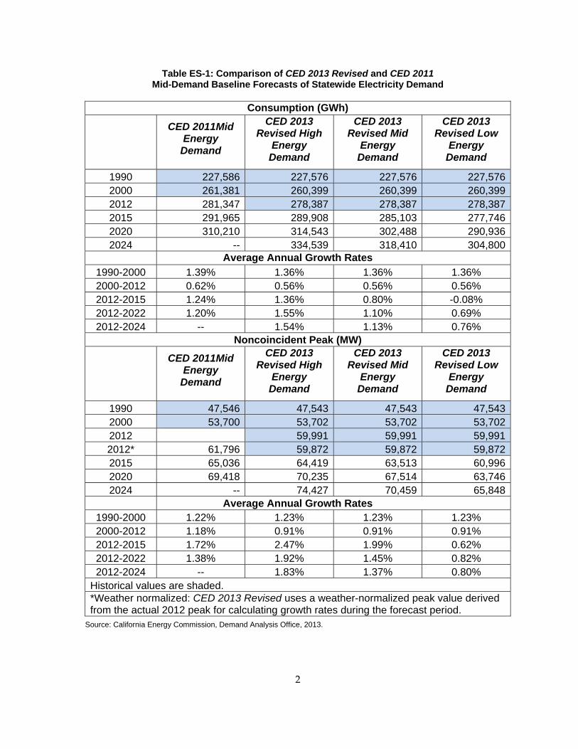
Baseline Electricity Forecast Results Table ES‐1 compares the CED 2013 Revised baseline forecast for selected years with the mid demand scenario from the previous Energy Commission adopted forecast, California Energy Demand 2012 – 2022 Final Forecast (CED 2011). Statewide electricity consumption begins the forecast period about 1 percent below CED 2011, as actual economic growth in California was slower than had been predicted in 2011. By 2020, consumption is around 2.5 percent lower in the mid demand case. The high demand case, with higher projected growth in consumption, matches the CED 2011 mid case by 2017. Statewide noncoincident peak demand, adjusted to account for atypical weather, is almost 3 percent lower than predicted in the CED 2011 mid case in 2012 but grows at a slightly higher rate from 2012 – 2022 in the mid case.

2

Table ES-1: Comparison of CED 2013 Revised and CED 2011 Mid-Demand Baseline Forecasts of Statewide Electricity Demand

Consumption (GWh)

CED 2011Mid

Energy Demand

CED 2013 Revised High

Energy Demand

CED 2013 Revised Mid

Energy Demand

CED 2013 Revised Low

Energy Demand

1990 227,586 227,576 227,576 227,5762000 261,381 260,399 260,399 260,3992012 281,347 278,387 278,387 278,3872015 291,965 289,908 285,103 277,7462020 310,210 314,543 302,488 290,9362024 -- 334,539 318,410 304,800

Average Annual Growth Rates 1990-2000 1.39% 1.36% 1.36% 1.36% 2000-2012 0.62% 0.56% 0.56% 0.56% 2012-2015 1.24% 1.36% 0.80% -0.08% 2012-2022 1.20% 1.55% 1.10% 0.69% 2012-2024 -- 1.54% 1.13% 0.76%

Noncoincident Peak (MW)

CED 2011Mid

Energy Demand


Energy Demand


Energy Demand


Energy Demand

1990 47,546 47,543 47,543 47,5432000 53,700 53,702 53,702 53,7022012 59,991 59,991 59,9912012* 61,796 59,872 59,872 59,8722015 65,036 64,419 63,513 60,9962020 69,418 70,235 67,514 63,7462024 -- 74,427 70,459 65,848

Average Annual Growth Rates 1990-2000 1.22% 1.23% 1.23% 1.23% 2000-2012 1.18% 0.91% 0.91% 0.91% 2012-2015 1.72% 2.47% 1.99% 0.62% 2012-2022 1.38% 1.92% 1.45% 0.82% 2012-2024 -- 1.83% 1.37% 0.80%

Historical values are shaded. *Weather normalized: CED 2013 Revised uses a weather-normalized peak value derived from the actual 2012 peak for calculating growth rates during the forecast period.

Source: California Energy Commission, Demand Analysis Office, 2013.

3

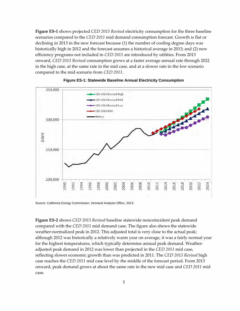
Figure ES‐1 shows projected CED 2013 Revised electricity consumption for the three baseline scenarios compared to the CED 2011 mid demand consumption forecast. Growth is flat or declining in 2013 in the new forecast because (1) the number of cooling degree days was historically high in 2012 and the forecast assumes a historical average in 2013; and (2) new efficiency programs not included in CED 2011 are introduced by utilities. From 2013 onward, CED 2013 Revised consumption grows at a faster average annual rate through 2022 in the high case, at the same rate in the mid case, and at a slower rate in the low scenario compared to the mid scenario from CED 2011.

Figure ES-1: Statewide Baseline Annual Electricity Consumption


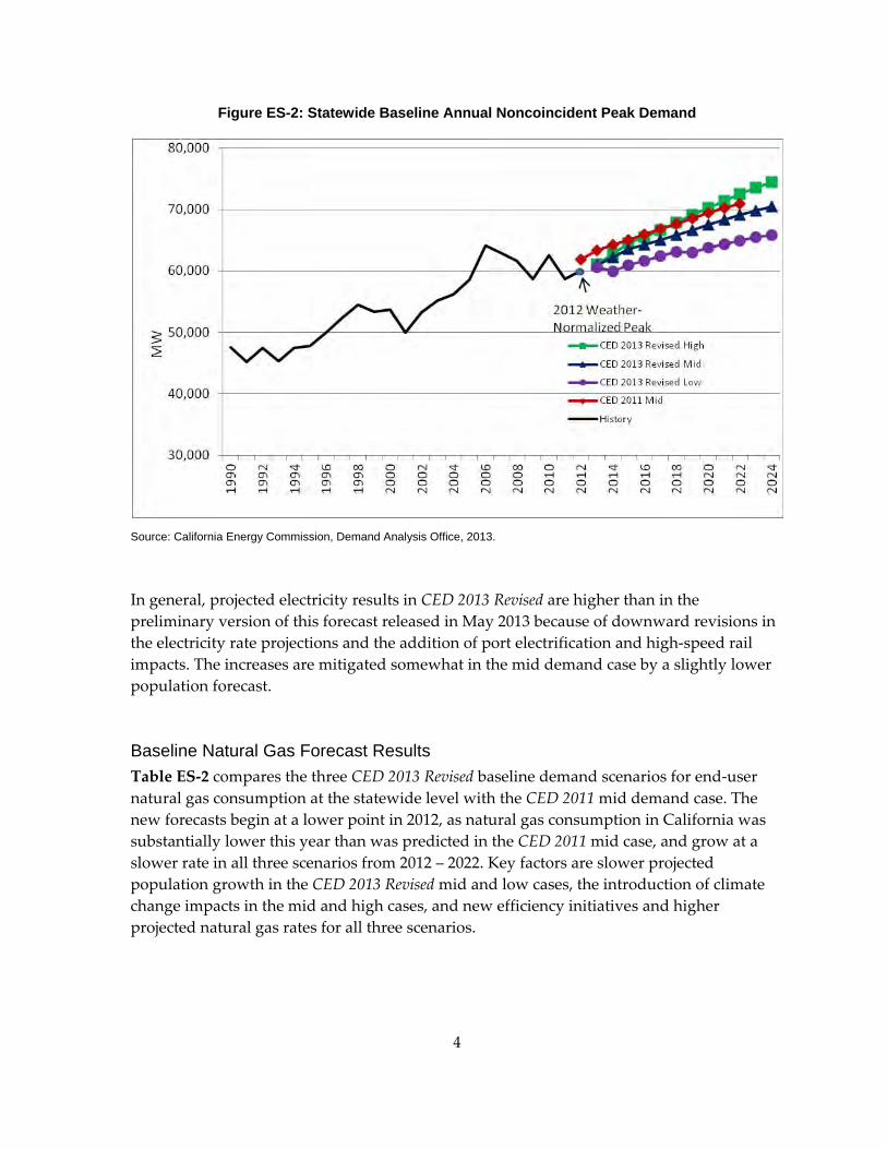
Figure ES‐2 shows CED 2013 Revised baseline statewide noncoincident peak demand compared with the CED 2011 mid demand case. The figure also shows the statewide weather‐normalized peak in 2012. This adjusted total is very close to the actual peak; although 2012 was historically a relatively warm year on average, it was a fairly normal year for the highest temperatures, which typically determine annual peak demand. Weather‐adjusted peak demand in 2012 was lower than projected in the CED 2011 mid case, reflecting slower economic growth than was predicted in 2011. The CED 2013 Revised high case reaches the CED 2011 mid case level by the middle of the forecast period. From 2013 onward, peak demand grows at about the same rate in the new mid case and CED 2011 mid case.

4

Figure ES-2: Statewide Baseline Annual Noncoincident Peak Demand


In general, projected electricity results in CED 2013 Revised are higher than in the preliminary version of this forecast released in May 2013 because of downward revisions in the electricity rate projections and the addition of port electrification and high‐speed rail impacts. The increases are mitigated somewhat in the mid demand case by a slightly lower population forecast.

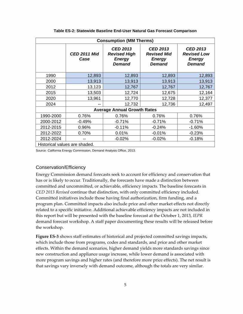
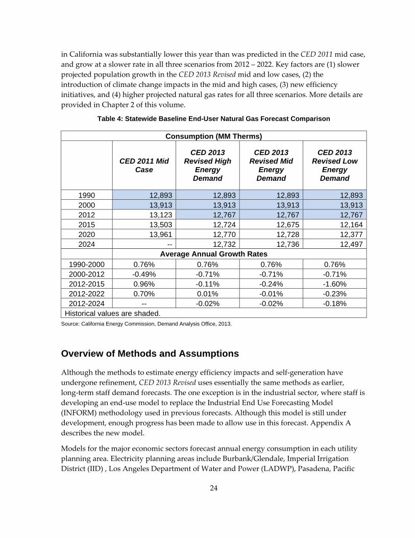
Baseline Natural Gas Forecast Results Table ES‐2 compares the three CED 2013 Revised baseline demand scenarios for end‐user natural gas consumption at the statewide level with the CED 2011 mid demand case. The new forecasts begin at a lower point in 2012, as natural gas consumption in California was substantially lower this year than was predicted in the CED 2011 mid case, and grow at a slower rate in all three scenarios from 2012 – 2022. Key factors are slower projected population growth in the CED 2013 Revised mid and low cases, the introduction of climate change impacts in the mid and high cases, and new efficiency initiatives and higher projected natural gas rates for all three scenarios.

5

Table ES-2: Statewide Baseline End-User Natural Gas Forecast Comparison

Consumption (MM Therms)

CED 2011 Mid Case


Energy Demand


Energy Demand


Energy Demand

1990 12,893 12,893 12,893 12,8932000 13,913 13,913 13,913 13,9132012 13,123 12,767 12,767 12,7672015 13,503 12,724 12,675 12,1642020 13,961 12,770 12,728 12,3772024 -- 12,732 12,736 12,497

Average Annual Growth Rates 1990-2000 0.76% 0.76% 0.76% 0.76% 2000-2012 -0.49% -0.71% -0.71% -0.71% 2012-2015 0.96% -0.11% -0.24% -1.60% 2012-2022 0.70% 0.01% -0.01% -0.23% 2012-2024 -- -0.02% -0.02% -0.18%

Historical values are shaded. Source: California Energy Commission, Demand Analysis Office, 2013.

Conservation/Efficiency Energy Commission demand forecasts seek to account for efficiency and conservation that has or is likely to occur. Traditionally, the forecasts have made a distinction between committed and uncommitted, or achievable, efficiency impacts. The baseline forecasts in CED 2013 Revised continue that distinction, with only committed efficiency included. Committed initiatives include those having final authorization, firm funding, and a program plan. Committed impacts also include price and other market effects not directly related to a specific initiative. Additional achievable efficiency impacts are not included in this report but will be presented with the baseline forecast at the October 1, 2013, IEPR demand forecast workshop. A staff paper documenting these results will be released before the workshop.

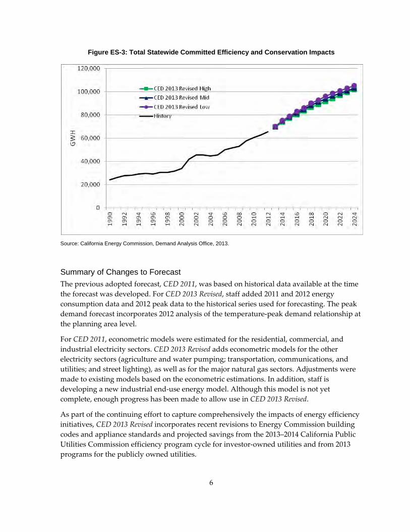
Figure ES‐3 shows staff estimates of historical and projected committed savings impacts, which include those from programs, codes and standards, and price and other market effects. Within the demand scenarios, higher demand yields more standards savings since new construction and appliance usage increase, while lower demand is associated with more program savings and higher rates (and therefore more price effects). The net result is that savings vary inversely with demand outcome, although the totals are very similar.

6

Figure ES-3: Total Statewide Committed Efficiency and Conservation Impacts


Summary of Changes to Forecast The previous adopted forecast, CED 2011, was based on historical data available at the time the forecast was developed. For CED 2013 Revised, staff added 2011 and 2012 energy consumption data and 2012 peak data to the historical series used for forecasting. The peak demand forecast incorporates 2012 analysis of the temperature‐peak demand relationship at the planning area level.

For CED 2011, econometric models were estimated for the residential, commercial, and industrial electricity sectors. CED 2013 Revised adds econometric models for the other electricity sectors (agriculture and water pumping; transportation, communications, and utilities; and street lighting), as well as for the major natural gas sectors. Adjustments were made to existing models based on the econometric estimations. In addition, staff is developing a new industrial end‐use energy model. Although this model is not yet complete, enough progress has been made to allow use in CED 2013 Revised.

As part of the continuing effort to capture comprehensively the impacts of energy efficiency initiatives, CED 2013 Revised incorporates recent revisions to Energy Commission building codes and appliance standards and projected savings from the 2013–2014 California Public Utilities Commission efficiency program cycle for investor‐owned utilities and from 2013 programs for the publicly owned utilities.

7

In addition to a predictive model to forecast residential adoption of photovoltaic systems and solar water heaters used in CED 2011, CED 2013 Revised employs a predictive model for the commercial sector that projects adoption of combined heat and power and photovoltaic systems. These models are based on methods used by the United States Energy Information Administration (U.S. EIA), as part of its National Energy Modeling System (NEMS), and the National Renewable Energy Laboratory (NREL).

CED 2011 included estimates of potential climate change impacts on peak demand. Along with an updated peak demand analysis, CED 2013 Revised incorporates estimates of climate change impacts on electricity and natural gas consumption. These impacts were developed using temperature scenarios provided by the Scripps Institute of Oceanography.

Stakeholders have expressed a strong interest in a more disaggregated demand forecast to better inform resource and infrastructure‐related analyses and decisions. As a first step in this direction, staff developed results at the climate zone level for CED 2013 Revised in addition to the usual utility planning area forecasts. The appropriate level of disaggregation for future forecasts, given data and other resource constraints, will be determined through internal discussions and input from stakeholders after the CED 2013 forecast cycle.

9

CHAPTER 1: Statewide Baseline Forecast Results and Methods Introduction

This California Energy Commission staff report presents forecasts of electricity and end‐user natural gas consumption and peak electricity demand for California and for each major utility planning area within the state for 2014 – 2024. The California Energy Demand 2014‐2024 Revised Forecast (CED 2013 Revised) supports the analysis and recommendations of the 2012 Integrated Energy Policy Report Update (2012 IEPR Update) and the 2013 Integrated Energy Policy Report (2013 IEPR), including electricity and natural gas system assessments and analysis of progress toward increased energy efficiency. This report details the historical and projected impacts of energy efficiency programs and standards as well as the effects of programs incentivizing distributed generation, continuing a major staff effort to improve the measurement and attribution of demand‐side impacts within the energy demand forecast.

The IEPR Lead Commissioner will conduct a workshop on October 1, 2013, to receive public comments on this forecast. Following the workshop, subject to the direction of the Lead Commissioner after considering public comments provided during the workshop comment period, staff will prepare a final forecast for adoption by the Energy Commission. The revised forecast will include an assessment of incremental uncommitted efficiency impacts not included in CED 2013 Revised.

The final forecasts will be used in a number of applications, including the California Public Utilities Commission (CPUC) 2014 Long Term Procurement Plan (LTPP). The CPUC has identified the Integrated Energy Policy Report (IEPR) process as “the appropriate venue for considering issues of load forecasting, resource assessment, and scenario analyses, to determine the appropriate level and ranges of resource needs for load serving entities in California.”1 The final forecasts will also be an input to California Independent System Operator (California ISO) controlled grid studies and other transmission planning studies and in the California Gas Report2 and electricity supply‐demand (resource adequacy) assessments.

CED 2013 Revised includes three full scenarios: a high energy demand case, a low energy demand case, and a mid energy demand case. The high energy demand case incorporates relatively high economic/demographic growth, relatively low electricity and natural gas rates, and

1 Peevey, Michael. September 9, 2004, Assigned Commissioner’s Ruling on Interaction Between the CPUC Long‐Term Planning Process and the California Energy Commission Integrated Energy Policy Report Process. Rulemaking 04‐04‐003.

2 California electric and gas utilities prepare the California Gas Report in compliance with CPUC Decision D.95‐01‐039.

10

relatively low efficiency program and self‐generation impacts. The low energy demand case includes lower economic/demographic growth, higher assumed rates, and higher efficiency program and self‐generation impacts. The mid case uses input assumptions at levels between the high and low cases. Details on input assumptions for these scenarios are provided later in this chapter. The forecast comparisons presented in this report show the three CED 2013 Revised cases versus the adopted California Energy Demand 2012 – 2022 Final Forecast3 (CED 2011) mid demand case, except where otherwise noted.

Before the October 1, 2013, workshop, staff will document and release in a staff paper estimates of additional achievable energy efficiency impacts for the investor‐owned utilities (IOUs) that are incremental to (do not overlap with) efficiency savings included in CED 2013 Revised. After the October 1 workshop, the forecasts presented in this report will be adjusted to account for this incremental efficiency. To avoid confusion between CED 2013 Revised forecasts and these (and future) forecasts adjusted to account for additional efficiency, results presented in this report will be referred to as baseline forecasts.

Summary of Changes to Forecast

The previous long‐run forecast, CED 2011, was based on 2011 peak demand and 2010 energy. For the current forecast, staff added 2011 and 2012 energy consumption data and 2012 peak data to the historical series used for forecasting. The peak demand forecast incorporates 2012 analysis of the temperature‐peak demand relationship at the planning area level.

For CED 2011, econometric models were estimated for the residential, commercial, and industrial electricity sectors. CED 2013 Revised adds econometric models for the other electricity sectors (agriculture and water pumping; transportation, communications, and utilities; and street lighting), as well as for the major natural gas sectors. This means that forecasts were developed in two ways: through the Energy Commission’s existing models and through econometric models. Adjustments were made to existing models based on the econometric estimations, and results from existing models were compared to econometric results. In addition, staff is developing a new industrial end‐use energy model. Although this model is not yet complete, enough progress has been made to allow use in CED 2013 Revised.

As part of the continuing effort to capture comprehensively the impacts of energy efficiency initiatives, CED 2013 Revised incorporates recent revisions to Energy Commission building codes and appliance standards, including projected effects from the 2013 updates to the

3 California Energy Commission. June 2012. California Energy Demand 2012 – 2022 Final Forecast. CEC‐200‐2012‐001‐CMF (Volumes 1 and 2). http://www.energy.ca.gov/2012publications/CEC‐200‐2012‐001/CEC‐200‐2012‐001‐CMF‐V1.pdf and http://www.energy.ca.gov/2012publications/CEC‐200‐2012‐001/CEC‐200‐2012‐001‐CMF‐V2.pdf.

11

Title 24 building standards and the battery charger standards, to be implemented in 2014. Utility program impacts were updated to include projected savings from the 2013 – 2014 CPUC efficiency program cycle for IOUs and from 2013 programs for the publicly owned utilities (POUs). Chapter 3 provides details on staff work related to efficiency impact measurement for this forecast.

Staff used a predictive model to forecast residential adoption of photovoltaic systems (PV) and solar water heaters for the first time in CED 2011. CED 2013 Revised also employs a predictive model for the commercial sector that projects adoption of combined heat and power (CHP) and PV systems. These models are based on methods used by the United States Energy Information Administration (U.S. EIA), as part of its National Energy Modeling System (NEMS), and the National Renewable Energy Laboratory (NREL). Details of the residential PV and commercial CHP and PV models are provided in Appendix B.

CED 2011 included estimates of potential climate change impacts on peak demand. Along with an updated peak demand analysis, CED 2013 Revised incorporates estimates of climate change impacts on electricity and natural gas consumption. These impacts were developed using temperature scenarios provided by the Scripps Institution of Oceanography. The Scripps Institution scenarios, and how they were included in the forecast, are discussed in Appendix A.

Stakeholders have expressed a strong interest in a more disaggregated demand forecast to better inform resource and infrastructure‐related analyses and decisions. As a first step in this direction, staff developed results at the climate zone level for CED 2013 Revised in addition to the usual planning area forecasts. Climate zone results are provided in the planning area chapters in Volume 2 of this report. The appropriate level of disaggregation for future forecasts, given data and other resource constraints, will be determined through internal discussions and input from stakeholders after the CED 2013 forecast cycle.

Changes From Preliminary to Revised Forecast

Staff prepared a preliminary forecast4 (CED 2013 Preliminary), presented in a workshop on May 30, 2013. The analysis for CED 2013 Revised reflects the following updates and changes:

• Updated economic/demographic projections based on forecasts by Moody’s and Global Insight for May 2013 (the preliminary forecast used projections from February 2011).

• Revised electricity and natural gas rate forecasts.

4 Kavalec, Chris, Nicholas Fugate, Bryan Alcorn, Mark Ciminelli, Asish Gautum, Kate Sullivan, and Malachi Weng‐Gutierrez, 2013. California Energy Demand 2014–2024 Preliminary Forecast, Volumes 1 and 2. California Energy Commission, Electricity Supply Analysis Division. CEC‐200‐2013‐004 SD‐VI and CEC‐200‐2013‐004 SD‐VII.

12

• New projections for port electrification and high‐speed rail, developed with the assistance of the Energy Commission’s Transportation Energy Office.

• Incorporation of a new commercial PV adoption component within the commercial self‐generation predictive model. The preliminary forecast relied on a trend analysis for this sector and technology.

• Updated estimates of historical and projected natural gas efficiency savings.

• Development of projected peak demand impacts from critical peak pricing and peak time rebate demand response programs.

• Development of scenarios will be developed for incremental achievable energy efficiency for electricity consumption and peak demand and natural gas consumption. This report provides the baseline forecast that will be adjusted to account for these additional savings.

In general, projected electricity results are higher than in the preliminary forecasts because of downward revisions in the electricity rate projections and the addition of port electrification and high‐speed rail impacts (discussed later in this chapter). The increases are mitigated somewhat in the mid demand case by a slightly lower population forecast. At the statewide level, electricity consumption is projected to be 2.1 percent, 1.8 percent, and 1.4 percent higher than in CED 2013 Preliminary by 2024 in the high, mid, and low demand scenarios, respectively. For peak demand, the 2024 increases are around 1.9 percent, 1.2 percent, and 1.1 percent.

CED 2013 Revised does not reflect significant change in projected natural gas rates in the mid and high demand cases, so the two gas forecasts are much closer for these two scenarios. (CED 2013 Revised is 0.3 percent and 0.5 percent lower, respectively, by 2024.) In the low demand scenario, natural gas rates are somewhat higher in CED 2013 Revised, around 10 to 15 percent, than CED 2013 Preliminary rates by 2024, and the new gas demand forecast is 1.7 percent lower in 2024.

Statewide Baseline Forecast Results

Table 1 compares the CED 2013 Revised baseline forecast for selected years with the CED 2011 mid demand case. For statewide electricity consumption, the new forecast begins about 1 percent below CED 2011 in 2012, reflecting less actual economic growth in California than had been predicted in 2011. Consumption in the new mid scenario grows at a slower rate through 2022 compared to the CED 2011 mid case as a result of lower projected population growth and the introduction of updated Title 24 and new Title 20 standards during the forecast period. By 2020, consumption is around 2.5 percent lower. In addition, consumption growth referenced to 2012 will be slower, all else equal, because this was a relatively warm year on average—warmer in general than forecasted years, which are based

13

on historical average weather. The high demand case, with higher projected growth in consumption, matches the CED 2011 mid case by 2017. Statewide noncoincident5 weather‐normalized6 peak demand is almost 3 percent lower than predicted in the CED 2011 mid case in 2012 but grows at a slightly higher rate from 2012‐2022 in the mid case.

The historical data used for this forecast differs slightly from CED 2011 as staff strives to improve processes to aggregate data submitted by utilities into the proper form required by the forecasting models. In addition, continuing review of self‐generation data has found cases where on‐site consumption was improperly estimated in the past.

5 The state’s coincident peak is the actual peak, while the noncoincident peak is the sum of actual peaks for the planning areas, which may occur at different times.

6 Peak demand is weather‐normalized in 2012 to provide the proper benchmark for comparison to future peak demand, which assumes either average (normalized) weather or hotter conditions measured relative to 2012 due to climate change.

14

Table 1: Comparison of CED 2013 Revised and CED 2011 Mid Case Demand Baseline Forecasts of Statewide Electricity Demand

Consumption (GWh)

CED 2011 Mid Energy Demand


Energy Demand


Energy Demand


Energy Demand

1990 227,586 227,576 227,576 227,5762000 261,381 260,399 260,399 260,3992012 281,347 278,387 278,387 278,3872015 291,965 289,908 285,103 277,7462020 310,210 314,543 302,488 290,9362024 -- 334,539 318,410 304,800

Average Annual Growth Rates 1990-2000 1.39% 1.36% 1.36% 1.36%2000-2012 0.62% 0.56% 0.56% 0.56%2012-2015 1.24% 1.36% 0.80% -0.08%2012-2022 1.20% 1.55% 1.10% 0.69%2012-2024 -- 1.54% 1.13% 0.76%

Noncoincident Peak (MW)



Energy Demand

CED 2013 Revised Energy

Demand


Energy Demand

1990 47,546 47,543 47,543 47,5432000 53,700 53,702 53,702 53,7022012 59,991 59,991 59,9912012* 61,796 59,872 59,872 59,8722015 65,036 64,419 63,513 60,9962020 69,418 70,235 67,514 63,7462024 -- 74,427 70,459 65,848

Average Annual Growth Rates 1990-2000 1.22% 1.23% 1.23% 1.23%2000-2012 1.18% 0.91% 0.91% 0.91%2012-2015 1.72% 2.47% 1.99% 0.62%2012-2022 1.38% 1.92% 1.45% 0.82%2012-2024 -- 1.83% 1.37% 0.80%

Historical values are shaded. *Weather normalized: CED 2013 Revised uses a weather-normalized peak value derived from the actual 2012 peak for calculating growth rates during the forecast period


15

Annual Electricity Consumption Figure 1 shows statewide historical electricity consumption, projected CED 2013 Revised baseline consumption for the three scenarios, and the CED 2011 mid case demand consumption forecast. Growth is flat or declining in 2013 in the new forecast because (1) the number of cooling degree days was historically high in 2012 and the forecast assumes a historical average in 2013; and (2) new efficiency programs not included in CED 2011 are introduced by utilities. From 2013 onward, CED 2013 Revised consumption grows at a faster average annual rate through 2022 in the high case (1.68 percent), at the same rate in the mid case (1.24 percent), and at a slower rate in the low scenario (0.90 percent) compared to CED 2011 mid case (1.24 percent).

Figure 1: Statewide Baseline Annual Electricity Consumption


As shown in Figure 2, CED 2013 Revised baseline per capita electricity consumption is projected to decrease from 2012 to 2013 because of flat total consumption growth combined with population increase. Thereafter, per capita consumption remains flat in the mid case scenario and declines in the low before rising slightly toward the end of the forecast period due to increasing electric vehicle use. The projected impacts of new efficiency initiatives keep the CED 2013 Revised mid case below CED 2011 through 2022. Higher economic/demographic growth in the high demand case increases per‐capita consumption throughout the forecast period, surpassing that in the CED 2011 mid case by 2015.

16

Figure 2: Statewide Baseline Electricity Annual Consumption per Capita


17

Table 2 compares projected baseline annual consumption in each scenario for the three major economic sectors—residential, commercial, and industrial (manufacturing, construction, and resource extraction)—with the CED 2011 mid demand case. Projected residential and commercial sector growth in the CED 2013 Revised mid case from 2012‐2022 is slower compared to the CED 2011 mid case, mainly because of a reversion to normal weather at the beginning of the forecast period from 2012, which was a historically warm year on average.

18

Table 2: Baseline Electricity Consumption by Sector

Residential Consumption (GWh)



Energy Demand


Energy Demand


Energy Demand

2012 91,934 90,649 90,649 90,6492015 95,520 96,229 94,056 91,3652020 104,853 108,231 101,991 97,1522024 -- 119,438 111,254 105,403

Average Annual Growth, Residential Sector 2012-2022 1.78% 2.30% 1.63% 1.10% 2013-2022 1.80% 2.58% 1.86% 1.40% 2012-2024 -- 2.32% 1.72% 1.26%

Commercial Consumption (GWh)



Energy Demand


Energy Demand


Energy Demand

2012 103,641 101,703 101,703 101,7032015 108,514 105,583 104,064 102,3922020 116,658 115,476 112,091 108,4702024 -- 121,826 117,486 113,804

Average Annual Growth, Commercial Sector 2012-2022 1.45% 1.58% 1.24% 0.92% 2013-2022 1.46% 1.72% 1.38% 1.04% 2012-2024 -- 1.52% 1.21% 0.94%

Industrial Consumption (GWh)



Energy Demand


Energy Demand


Energy Demand

2012 47,943 47,614 47,614 47,6142015 49,276 48,850 47,986 45,8812020 49,194 49,947 47,979 45,4512024 -- 50,797 47,920 44,636

Average Annual Growth, Industrial Sector 2012-2022 0.14% 0.56% 0.08% -0.54% 2012-2024 -- 0.54% 0.05% -0.54% Historical values are shaded. Source: California Energy Commission, Demand Analysis Office, 2013.

19

To compare across weather‐normalized years, growth rates for 2013 – 2022 are also shown for the residential and commercial sectors; the rates of growth for the two residential and commercial mid cases are much closer when examining this period. The effect of lower population growth versus CED 2011 on residential consumption is partially offset by higher per capita income, since personal income is projected to be about the same in the previous and new mid cases (see Figure 7), with a lower population in the latter. In addition, unlike CED 2011, the CED 2013 Revised residential and commercial forecasts include projected consumption impacts from climate change that are increasing throughout the forecast period. Average annual growth in industrial consumption from 2012 – 2022 is slightly lower in the CED 2013 Revised mid case than in the previous forecast, reflecting lower projected growth in resource extraction and construction.

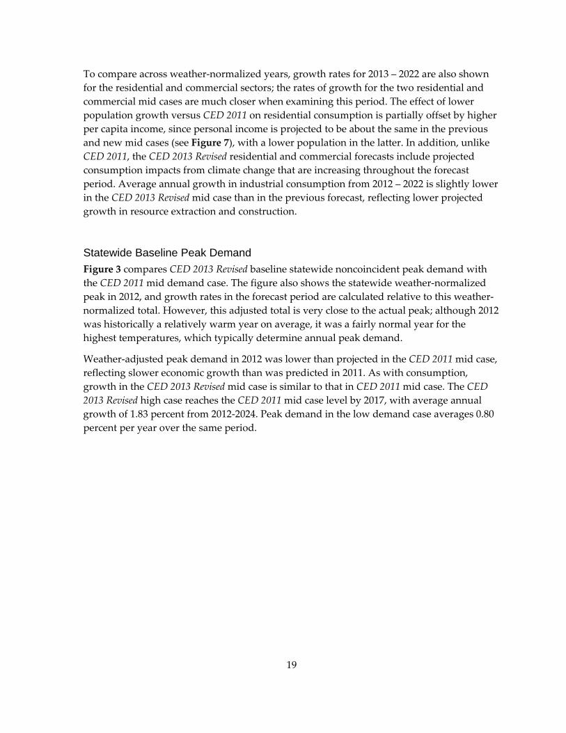
Statewide Baseline Peak Demand Figure 3 compares CED 2013 Revised baseline statewide noncoincident peak demand with the CED 2011 mid demand case. The figure also shows the statewide weather‐normalized peak in 2012, and growth rates in the forecast period are calculated relative to this weather‐normalized total. However, this adjusted total is very close to the actual peak; although 2012 was historically a relatively warm year on average, it was a fairly normal year for the highest temperatures, which typically determine annual peak demand.

Weather‐adjusted peak demand in 2012 was lower than projected in the CED 2011 mid case, reflecting slower economic growth than was predicted in 2011. As with consumption, growth in the CED 2013 Revised mid case is similar to that in CED 2011 mid case. The CED 2013 Revised high case reaches the CED 2011 mid case level by 2017, with average annual growth of 1.83 percent from 2012‐2024. Peak demand in the low demand case averages 0.80 percent per year over the same period.

20

Figure 3: Statewide Baseline Annual Noncoincident Peak Demand


Figure 4 shows baseline load factors for the state as a whole. The load factor represents the relationship between average energy demand and peak. The smaller the load factor, the greater is the difference between peak and average hourly demand. The load factor varies with temperature; in years with extreme heat (1998, 2006), demand is “peakier,” which results in lower system load factors.

The general declining trend in the load factor over the last 20 years indicates a greater proportion of homes and businesses with central air conditioning. These trends are projected to continue over most of the forecast period for all three demand scenarios (as in CED 2011). Energy efficiency measures, such as more efficient lighting, contribute to the declining load factor by reducing energy use while having an insignificant effect on peak. Late in the forecast period, projected increasing numbers of electric vehicles, which are assumed to affect consumption much more than peak demand, begin to push load factors upward.

21

Figure 4: Statewide Baseline Noncoincident Peak Load Factors


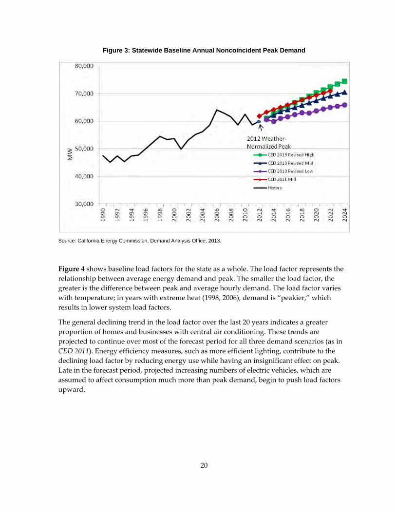
Figure 5 shows historical and projected baseline noncoincident peak demand per capita and reflects the results for total peak demand in Figure 3. Continued increases in air conditioner usage yield growth through most of the forecast period in the CED 2013 Revised mid and high cases. In the low demand case, lower total peak demand combined with population projections that are relatively close to those in the mid case (see Figure 9) push peak per capita far below the other two demand cases.

22

Figure 5: Statewide Baseline Noncoincident Peak Demand per Capita


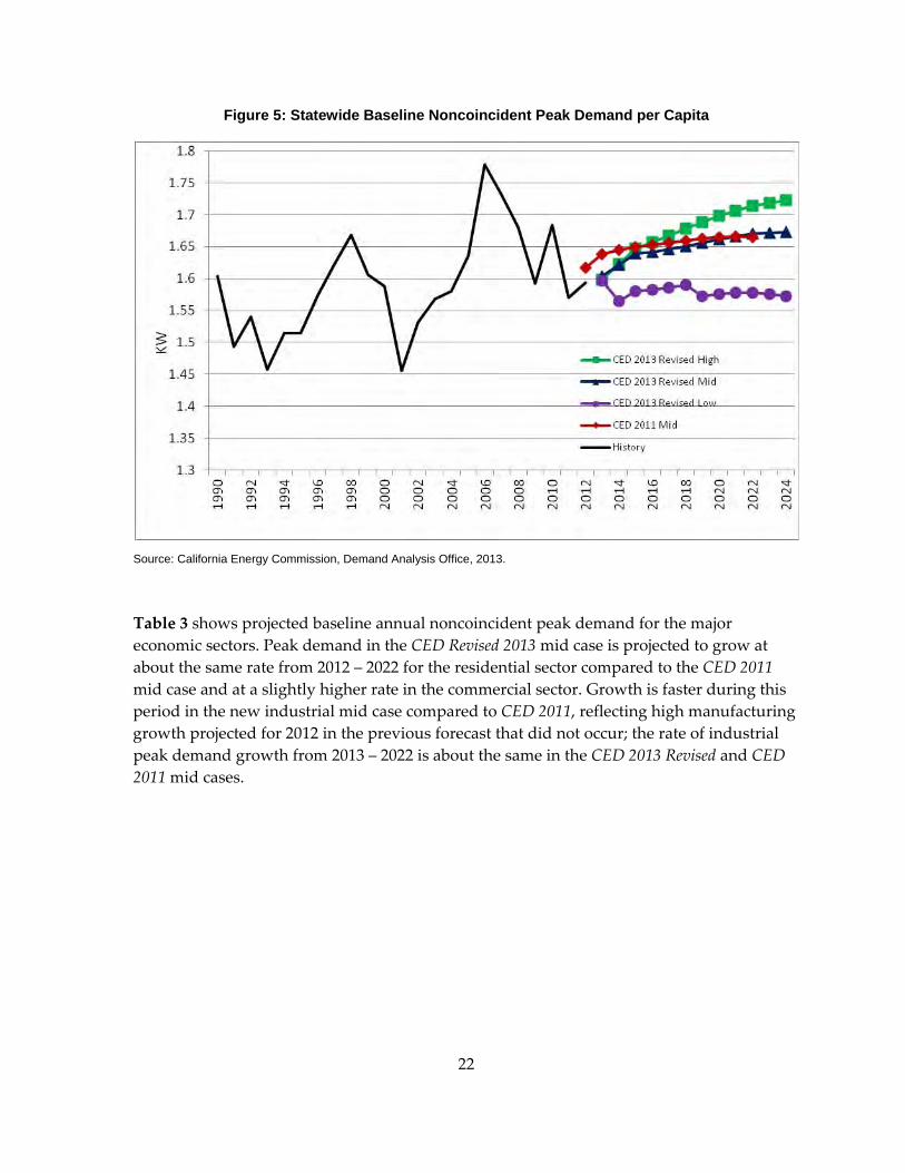
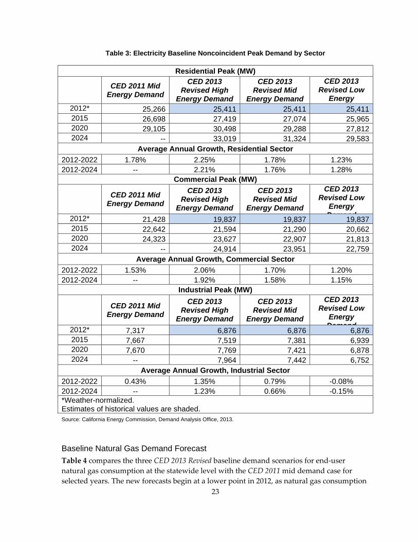
Table 3 shows projected baseline annual noncoincident peak demand for the major economic sectors. Peak demand in the CED Revised 2013 mid case is projected to grow at about the same rate from 2012 – 2022 for the residential sector compared to the CED 2011 mid case and at a slightly higher rate in the commercial sector. Growth is faster during this period in the new industrial mid case compared to CED 2011, reflecting high manufacturing growth projected for 2012 in the previous forecast that did not occur; the rate of industrial peak demand growth from 2013 – 2022 is about the same in the CED 2013 Revised and CED 2011 mid cases.

23

Table 3: Electricity Baseline Noncoincident Peak Demand by Sector

Residential Peak (MW)



Energy Demand


Energy Demand


Energy 2012* 25,266 25,411 25,411 25,4112015 26,698 27,419 27,074 25,9652020 29,105 30,498 29,288 27,8122024 -- 33,019 31,324 29,583

Average Annual Growth, Residential Sector 2012-2022 1.78% 2.25% 1.78% 1.23% 2012-2024 -- 2.21% 1.76% 1.28%

Commercial Peak (MW)



Energy Demand


Energy Demand


Energy Demand2012* 21,428 19,837 19,837 19,837

2015 22,642 21,594 21,290 20,6622020 24,323 23,627 22,907 21,8132024 -- 24,914 23,951 22,759

Average Annual Growth, Commercial Sector 2012-2022 1.53% 2.06% 1.70% 1.20% 2012-2024 -- 1.92% 1.58% 1.15%

Industrial Peak (MW)



Energy Demand


Energy Demand


Energy Demand2012* 7,317 6,876 6,876 6,876

2015 7,667 7,519 7,381 6,9392020 7,670 7,769 7,421 6,8782024 -- 7,964 7,442 6,752

Average Annual Growth, Industrial Sector 2012-2022 0.43% 1.35% 0.79% -0.08% 2012-2024 -- 1.23% 0.66% -0.15% *Weather-normalized. Estimates of historical values are shaded. Source: California Energy Commission, Demand Analysis Office, 2013.

Baseline Natural Gas Demand Forecast Table 4 compares the three CED 2013 Revised baseline demand scenarios for end‐user natural gas consumption at the statewide level with the CED 2011 mid demand case for selected years. The new forecasts begin at a lower point in 2012, as natural gas consumption

24

in California was substantially lower this year than was predicted in the CED 2011 mid case, and grow at a slower rate in all three scenarios from 2012 – 2022. Key factors are (1) slower projected population growth in the CED 2013 Revised mid and low cases, (2) the introduction of climate change impacts in the mid and high cases, (3) new efficiency initiatives, and (4) higher projected natural gas rates for all three scenarios. More details are provided in Chapter 2 of this volume.

Table 4: Statewide Baseline End-User Natural Gas Forecast Comparison


CED 2011 Mid Case


Energy Demand


Energy Demand


Energy Demand

1990 12,893 12,893 12,893 12,8932000 13,913 13,913 13,913 13,9132012 13,123 12,767 12,767 12,7672015 13,503 12,724 12,675 12,1642020 13,961 12,770 12,728 12,3772024 -- 12,732 12,736 12,497



Overview of Methods and Assumptions

Although the methods to estimate energy efficiency impacts and self‐generation have undergone refinement, CED 2013 Revised uses essentially the same methods as earlier, long‐term staff demand forecasts. The one exception is in the industrial sector, where staff is developing an end‐use model to replace the Industrial End Use Forecasting Model (INFORM) methodology used in previous forecasts. Although this model is still under development, enough progress has been made to allow use in this forecast. Appendix A describes the new model.

Models for the major economic sectors forecast annual energy consumption in each utility planning area. Electricity planning areas include Burbank/Glendale, Imperial Irrigation District (IID) , Los Angeles Department of Water and Power (LADWP), Pasadena, Pacific

25

Gas and Electric (PG&E), Southern California Edison (SCE), San Diego Gas & Electric (SDG&E), and the Sacramento Municipal Utility District (SMUD). Natural gas planning areas include PG&E, SDG&E, and the Southern California Gas Company (SoCalGas). After adjusting for historical weather and usage, the annual consumption forecast is used to project annual peak demand. The commercial, residential, and industrial sector energy models are structural models that attempt to explain how energy is used by process and end use. Structural models are critical in accounting for the forecasted impacts of mandatory energy efficiency standards and other energy efficiency programs that seek to encourage adoption of more efficient technologies by end users. The forecasts of agricultural and water pumping energy consumption are made using econometric methods for individual subsectors (for example, dairy and livestock). Projections for the transportation, communications, and utilities (TCU) and street lighting sectors rely on trend analyses. A detailed discussion of forecast methods and data sources is available in the 2005 Methods Report.7 The commercial end‐use forecast is supported by projections of floor space by building type (restaurant, retail, and so on), which are estimated using regressions that include various economic and demographic indicators as explanatory variables.8

In addition to existing models, staff incorporated econometric model estimation and forecast results from models estimated for total peak demand and for electricity and natural gas consumption in all sectors except for TCU gas, where the natural gas consumption data did not yield a parsimonious (simple formulation with high explanatory power) model. Estimation results for the econometric models are provided in Appendix C.

Results from the econometric estimations were applied to existing models in the following manner:

• Electricity price elasticities of demand9 for the residential end‐use and industrial models for both electricity and natural gas were changed to be consistent with elasticities estimated for the residential, manufacturing, and resource extraction/construction econometric models.

• The electricity forecast for the manufacturing sector was adjusted to reflect a trend in efficiency improvement estimated for the manufacturing econometric model.

• Results from the Hourly Electricity Load Model, used to forecast annual peak demand in each planning area, were adjusted to incorporate climate change scenarios using results from the peak econometric model.

7 California Energy Commission. June 2005. Energy Demand Forecast Methods Report, CEC‐400‐2005‐036. http://www.energy.ca.gov/2005publications/CEC‐400‐2005‐036/CEC‐400‐2005‐036.PDF

8 As an example, projections for retail floor space are based on regressions that include personal income and retail employment.

9 Price elasticities of demand measure the responsiveness of demand to changes in price and are discussed further in Appendix A.

26

• Results for the residential, commercial, industrial, and agricultural forecasts were adjusted to incorporate climate change using results from the sector econometric models.

• High and low scenarios were developed for the agricultural/water pumping, TCU (electricity only), and street lighting sectors using the new econometric models benchmarked to the single scenarios output from the existing models. (CED 2011 included only one scenario for these sectors.)

• Planning area forecasts for all sectors were broken out into climate zones using the econometric models. Econometric climate zone results were benchmarked to planning area totals by sector.

Although staff used existing models for this forecast (except as noted in the bullets previously listed), a comparison with econometric results is provided here at the statewide level and in Appendix A for individual planning areas.

For the high demand scenario, electricity consumption in the pure econometric forecast was 1.2 percent higher and peak demand 1.8 percent higher in 2024 compared to CED 2013 Revised statewide results shown in this chapter. The mid demand econometric scenario yielded projected 2024 consumption 1.9 percent higher than CED 2013 Revised, while peak demand was 2.0 percent higher. Differences were slightly higher in the low demand case, with both statewide consumption and peak demand projected to be 3.1 percent higher than CED 2013 Revised in 2024.

Given the manner efficiency is treated in each method, these results are to be expected. The end‐use models used in CED 2013 Revised account for historical and projected efficiency impacts explicitly while the econometric models implicitly account for historical efficiency trends that are then projected forward.10 If one presumes that energy efficiency efforts have intensified in recent years and into the near future, the econometric models, accounting for average trends from 1980 onward, would likely understate future efficiency impacts and therefore overstate demand. Future work to explicitly capture efficiency impacts in econometric estimations at the Energy Commission and through the CPUC’s macro consumption econometric project11 should allow better comparisons of end use and econometric results in the future.

The natural gas full econometric forecast12 is higher than CED 2013 Revised in all three scenarios by larger percentages. By 2024, the high demand econometric case is around 9

10 Econometric results were adjusted to account for only electric vehicles and other electrification and, in the case of peak demand, photovoltaic adoption beyond 2012 levels.

11 CPUC. October 28, 2010. Decision on Evaluation, Measurement, and Verification of California Energy Efficiency Programs. Decision 10‐10‐033.

12 Excluding TCU gas, where the CED 2013 Revised forecast was used.

27

percent higher, the mid econometric forecast about 6 percent higher, and the low econometric case around 7 percent higher. As with electricity, the difference is likely from omission of explicit program and standards impacts in the econometric forecast. As a percentage of usage, natural gas efficiency savings are higher compared to electricity; therefore, it is not surprising that the econometric forecasts should overstate consumption relative to CED 2013 Revised by larger percentages.

Economic and Demographic Assumptions California’s economy has been slowly recovering from the recession. In the last two years, the state has seen payroll gains, lower unemployment, fewer mortgage defaults, a dwindling inventory of homes for sale, and the return of tourism. Some characteristics of the current California economy include:13

• California’s recovery is gaining momentum on the strength of real estate, tech, and other services.

• Construction is pushing growth in payrolls. Construction employment is up almost 20,000 from a year earlier on a seasonally unadjusted basis.

• The unemployment rate is below 9 percent.

• Reinvigorated housing‐related industries should help push the unemployment rate below 8 percent.

• There is a significant reduction of distressed housing throughout the state.

• The inventory of houses for sale is at the lowest level since the middle of 2005 and is driving housing price gains.

• Improving labor markets and renewed household formations will drive new residential construction in the near term.

• The economic slowdown of China has softened the state’s exports.

• Alternative‐energy technologies are expected to play a part in the recovery. California is well‐suited to benefit from each part of the industry.

For the rest of 2013, the state’s economy is anticipated to grow at a moderate pace with construction and business services posting the largest payroll gains. During this recovery, California should be the target for venture‐capital investment because of California’s highly educated workforce.

Moody’s Analytics (Moody’s) and IHS Global Insight provided economic projections. In general, the forecasting methods are similar for both. Econometric equations are developed

13 Economic characteristics are based on summaries provided by Moody’s and IHS Global Insight in August 2013.

28

at the sectoral level (for example, consumer spending), adjustments are made based on the latest economic news and professional judgment, a national forecast is generated, and individual state and county forecasts are broken out. Staff uses the county forecasts to generate projections at the planning area and climate zone levels.

These two companies update their long‐term forecasts monthly; staff used the May 2013 projections for CED 2013 Revised. Other entities, such as University of California, Los Angeles (Anderson Forecast14) and the University of the Pacific,15 also project the leading economic indicators for California but do not provide the detail or length of forecast period required by Energy Commission demand forecasts.

For its May 2013 economic forecast, Moody’s generated seven scenarios:

• Baseline

• Stronger (compared to Baseline) Near‐Term Rebound

• Mild Second Recession

• Deeper Second Recession

• Protracted Slump

• Below‐Trend Long‐Term Growth

• Oil Price Increase, Dollar Crash, Inflation

IHS Global Insight provided three scenarios for its May 2013 forecast:

• Optimistic

• Baseline

• Pessimistic

As in CED 2013 Preliminary, staff selected the Global Insight Optimistic economic case for the high demand scenario and a mixture of Moody’s Mild Second Recession and Below‐Trend Long‐Term Growth cases for the low demand scenario. The two Moody’s cases were combined so that the Second Recession scenario drove the short‐term results (through 2018) and the Below‐Trend Long‐Term Growth case the longer‐term. The high and low demand scenarios as constructed, in general, project the highest and lowest rates of economic growth, respectively, of the various scenarios provided by the two companies throughout the forecast period. Moody’s Baseline economic forecast was used for the mid energy demand scenario.

14 http://uclaforecast.com/.

15 http://forecast.pacific.edu/.

29

Table 5 provides the key assumptions used by the two companies to develop the three economic scenarios. The probability assigned by Moody’s to the mid demand scenario (Moody’s Baseline) is 50 percent; that is, there is a 50 percent probability economic conditions will be worse than in this scenario. The equivalent probability for both Moody’s scenarios used in the low demand scenario is 4 – 5 percent. Global Insight portrays the probabilities somewhat differently: “The probability of being near” the Optimistic economic scenario is 10 percent.16

Table 5: Key Assumptions Embodied in Economic Scenarios

High Demand Scenario (IHS Global Insight Optimistic

Scenario), May 2013

Mid Demand Scenario (Moody’s Analytics Baseline

Scenario), May 2013

Low Demand Scenario (Combination of Moody’s

Analytics Second Recession and Below-Trend Long-Term Growth Scenarios), May 2013

National unemployment rate falls to 6.5 percent by early 2014.

National unemployment rate stays below 8 percent through 2017.

The unemployment rate is expected to hit a peak of 10.6 percent at the end of 2014.

There are no exits from the Eurozone, as members take decisive steps toward a banking and fiscal union that stabilize markets.

Some continued turmoil in Europe and weaker growth in the emerging world.

European recession deepens as Greece leaves the Eurozone and investors continue to worry about Portugal and Spain.

National light-duty vehicle sales reach more than 17 million in 2014.

National light-duty vehicle sales are above 16 million in 2014.

Unit auto sales decline throughout 2013 to a trough of only 13 million in early 2014.

National housing starts improve to near 1.25 million units by the end of 2013.

National housing starts are expected to break 2 million units by 2015.

House prices will experience a second decline, cumulatively falling 9 percent from the second quarter of 2013 to the third quarter of 2014.

Same as in mid demand scenario.

Oil and gas prices are expected to trend higher, just outpacing inflation.

Oil and gas prices fall in the short term.

The Federal Reserve halts its latest quantitative easing program before the end of 2013 and raises the federal funds rate in the second quarter of 2014.

The Federal Reserve is not expected to begin increasing interest rates until the unemployment rate has fallen to near 6.5 percent, around early 2015.

The Fed keeps the fed funds target rate near 0 percent until the fourth quarter of 2015.

The sequester spending cuts remain in place through the second quarter, but Congress agrees on a credible long-term deficit-reduction plan, replacing the automatic cuts.

The sequester will reduce outlays in 2013 by $58 billion and by $1.2 trillion over the next decade. Fiscal policy will subtract 1.4 percentage points from 2013 real GDP growth.

The negative impacts from longer-term spending issues rise significantly, causing the economy to descend into a second recession in the third quarter of 2013.

Source: Moody’s and IHS Global Insight, 2013.

16 E‐mail communication with Jim Diffley, IHS Global Insight, January 24, 2012.

30

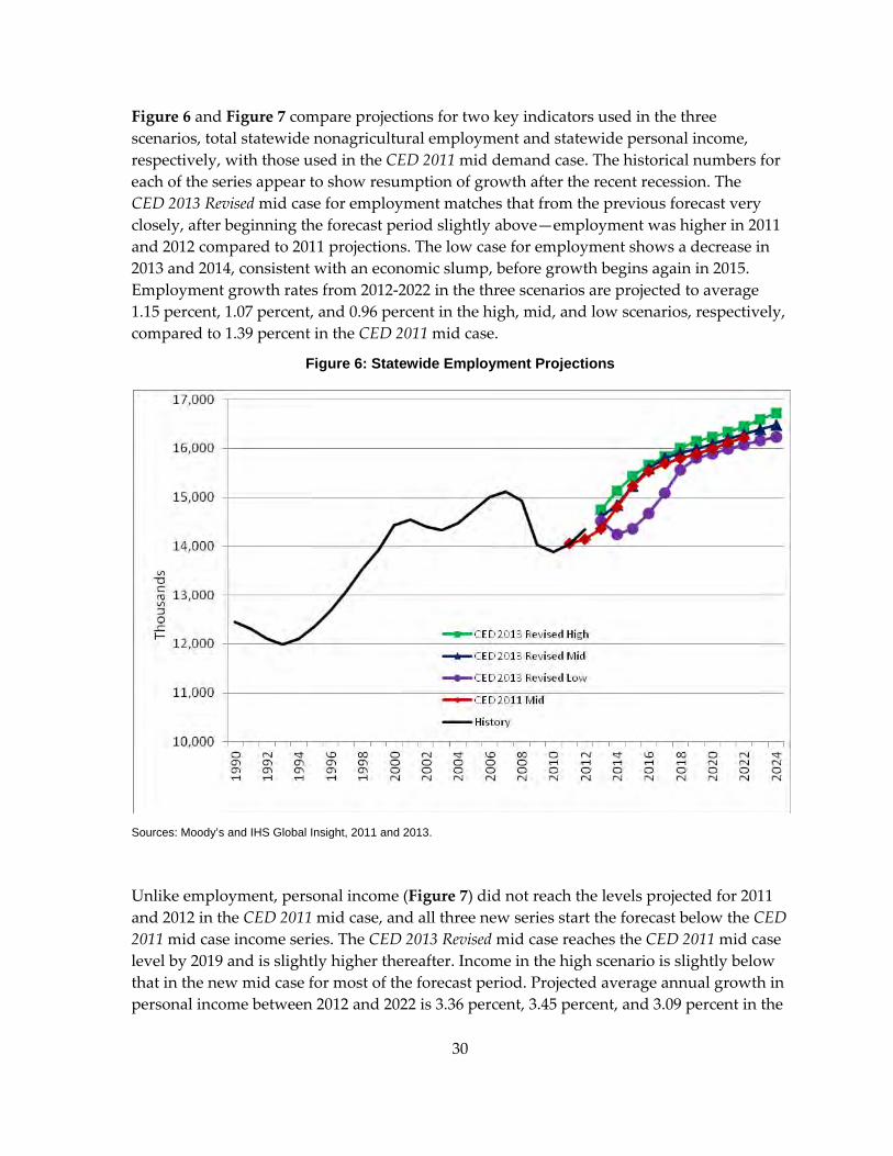
Figure 6 and Figure 7 compare projections for two key indicators used in the three scenarios, total statewide nonagricultural employment and statewide personal income, respectively, with those used in the CED 2011 mid demand case. The historical numbers for each of the series appear to show resumption of growth after the recent recession. The CED 2013 Revised mid case for employment matches that from the previous forecast very closely, after beginning the forecast period slightly above—employment was higher in 2011 and 2012 compared to 2011 projections. The low case for employment shows a decrease in 2013 and 2014, consistent with an economic slump, before growth begins again in 2015. Employment growth rates from 2012‐2022 in the three scenarios are projected to average 1.15 percent, 1.07 percent, and 0.96 percent in the high, mid, and low scenarios, respectively, compared to 1.39 percent in the CED 2011 mid case.

Figure 6: Statewide Employment Projections

Sources: Moody’s and IHS Global Insight, 2011 and 2013.

Unlike employment, personal income (Figure 7) did not reach the levels projected for 2011 and 2012 in the CED 2011 mid case, and all three new series start the forecast below the CED 2011 mid case income series. The CED 2013 Revised mid case reaches the CED 2011 mid case level by 2019 and is slightly higher thereafter. Income in the high scenario is slightly below that in the new mid case for most of the forecast period. Projected average annual growth in personal income between 2012 and 2022 is 3.36 percent, 3.45 percent, and 3.09 percent in the

31

high, mid, and low demand scenarios, respectively, compared to 3.25 percent in the CED 2011 mid case.

Figure 7: Statewide Personal Income Projections

Sources: Moody’s and IHS Global Insight, 2011 and 2013.

Staff also developed scenario projections for number of households, shown in Figure 8, using the population projections discussed below and varying expected average persons per household. For the low demand case (higher persons per household), staff fit an exponential growth curve to historical persons per household for 1990‐2010. The mid case assumed half of the growth of the low demand case and the high case (lower persons per household) used Moody’s projections.17 The CED 2013 Revised number of households in the mid demand case grows more slowly than in CED 2011 due to lower projected population growth.

17 Moody’s projections for persons per household have typically been lower than historical trends.

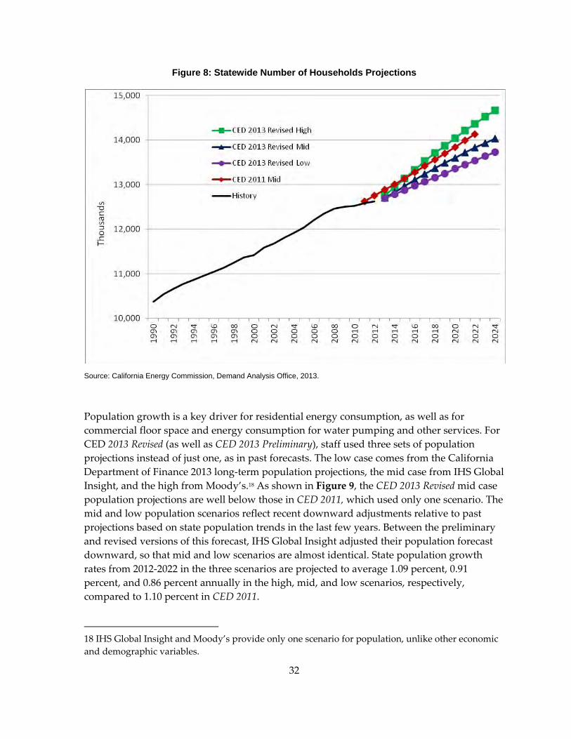
32

Figure 8: Statewide Number of Households Projections


Population growth is a key driver for residential energy consumption, as well as for commercial floor space and energy consumption for water pumping and other services. For CED 2013 Revised (as well as CED 2013 Preliminary), staff used three sets of population projections instead of just one, as in past forecasts. The low case comes from the California Department of Finance 2013 long‐term population projections, the mid case from IHS Global Insight, and the high from Moody’s.18 As shown in Figure 9, the CED 2013 Revised mid case population projections are well below those in CED 2011, which used only one scenario. The mid and low population scenarios reflect recent downward adjustments relative to past projections based on state population trends in the last few years. Between the preliminary and revised versions of this forecast, IHS Global Insight adjusted their population forecast downward, so that mid and low scenarios are almost identical. State population growth rates from 2012‐2022 in the three scenarios are projected to average 1.09 percent, 0.91 percent, and 0.86 percent annually in the high, mid, and low scenarios, respectively, compared to 1.10 percent in CED 2011.

18 IHS Global Insight and Moody’s provide only one scenario for population, unlike other economic and demographic variables.

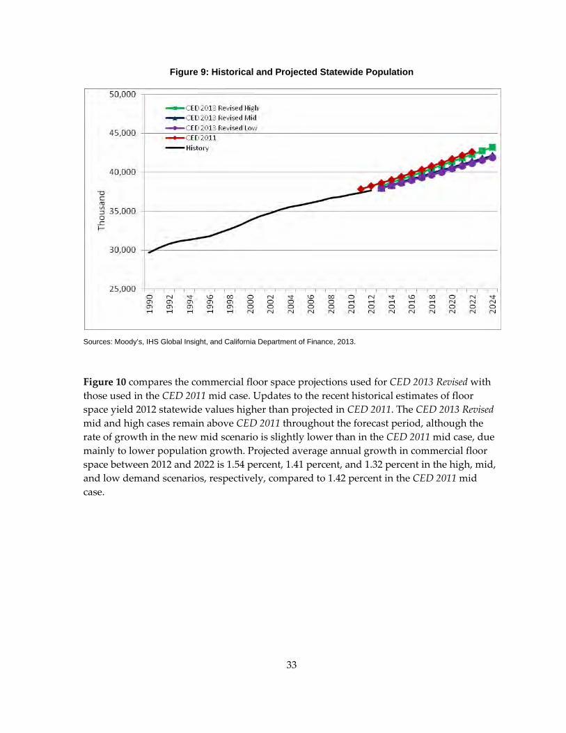
33

Figure 9: Historical and Projected Statewide Population

Sources: Moody’s, IHS Global Insight, and California Department of Finance, 2013.

Figure 10 compares the commercial floor space projections used for CED 2013 Revised with those used in the CED 2011 mid case. Updates to the recent historical estimates of floor space yield 2012 statewide values higher than projected in CED 2011. The CED 2013 Revised mid and high cases remain above CED 2011 throughout the forecast period, although the rate of growth in the new mid scenario is slightly lower than in the CED 2011 mid case, due mainly to lower population growth. Projected average annual growth in commercial floor space between 2012 and 2022 is 1.54 percent, 1.41 percent, and 1.32 percent in the high, mid, and low demand scenarios, respectively, compared to 1.42 percent in the CED 2011 mid case.

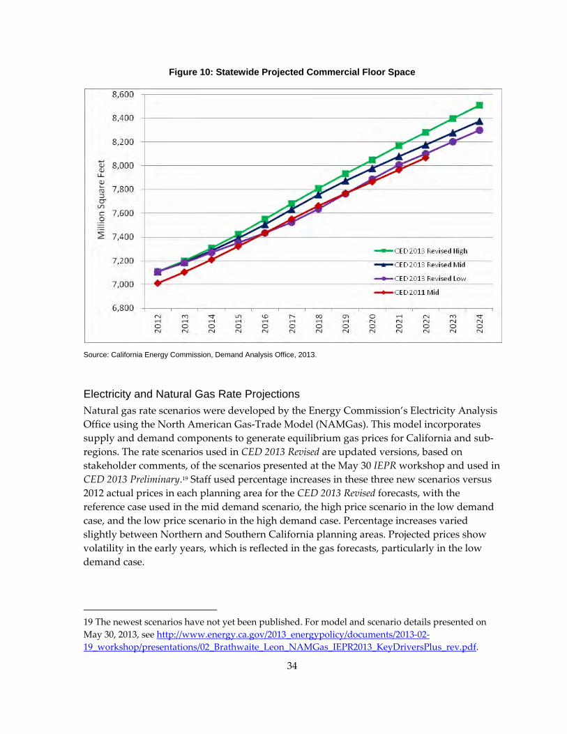
34

Figure 10: Statewide Projected Commercial Floor Space


Electricity and Natural Gas Rate Projections Natural gas rate scenarios were developed by the Energy Commission’s Electricity Analysis Office using the North American Gas‐Trade Model (NAMGas). This model incorporates supply and demand components to generate equilibrium gas prices for California and sub‐regions. The rate scenarios used in CED 2013 Revised are updated versions, based on stakeholder comments, of the scenarios presented at the May 30 IEPR workshop and used in CED 2013 Preliminary.19 Staff used percentage increases in these three new scenarios versus 2012 actual prices in each planning area for the CED 2013 Revised forecasts, with the reference case used in the mid demand scenario, the high price scenario in the low demand case, and the low price scenario in the high demand case. Percentage increases varied slightly between Northern and Southern California planning areas. Projected prices show volatility in the early years, which is reflected in the gas forecasts, particularly in the low demand case.

19 The newest scenarios have not yet been published. For model and scenario details presented on May 30, 2013, see http://www.energy.ca.gov/2013_energypolicy/documents/2013‐02‐19_workshop/presentations/02_Brathwaite_Leon_NAMGas_IEPR2013_KeyDriversPlus_rev.pdf.

35

As in CED 2013 Preliminary, the electricity price forecasts were generated using the Energy and Environmental Economics (E3) calculator.20 The E3 calculator allows users to create electricity price scenarios by inputting assumptions for efficiency savings, natural gas rates, amount of renewables, amount of combined heat and power, penetration of PV systems, level of demand response, and price regime (cap and trade). Between CED 2013 Preliminary and CED 2013 Revised, staff updated various inputs to the model, resulting in significantly lower projected electricity rates compared to the preliminary forecast. Modifications made by staff include:

• Updating the auction price estimates for cap and trade.

• Reducing the estimates of renewable resources needed for Renewables Portfolio Standard compliance and assigning scenarios to be consistent with demand outcomes.

• Incorporating the distribution of carbon allowance auction revenues back to ratepayers.

• Reducing transmission and distribution costs to reflect growth rates more consistent with other analyses, including California ISO Transmission Planning and the CPUC LTPP.

Table 6 summarizes the assumptions used to generate rate growth for each of the three demand scenarios. Efficiency and PV assumptions are based on CED 2011 results. CHP assumptions come from work for the Energy Commission by ICF International.21 Renewables numbers were taken from CPUC/Energy Commission joint scenario development for the 2012 LTPP.22

20 Available at http://www.ethree.com/public_projects/cpuc2.html.

21 Hedman, Bruce, Ken Darrow, Eric Wong, Anne Hampson. ICF International, Inc. 2012. Combined Heat and Power: 2011‐2030 Market Assessment. California Energy Commission. CEC‐200‐2012‐002. http://www.energy.ca.gov/2012publications/CEC‐200‐2012‐002/CEC‐200‐2012‐002.pdf.

22 http://www.cpuc.ca.gov/NR/rdonlyres/1A44BC30‐8C7A‐4400‐AEC8‐4A33363352AC/0/2013TPPRPSPortfoliostransmittalletter.pdf.

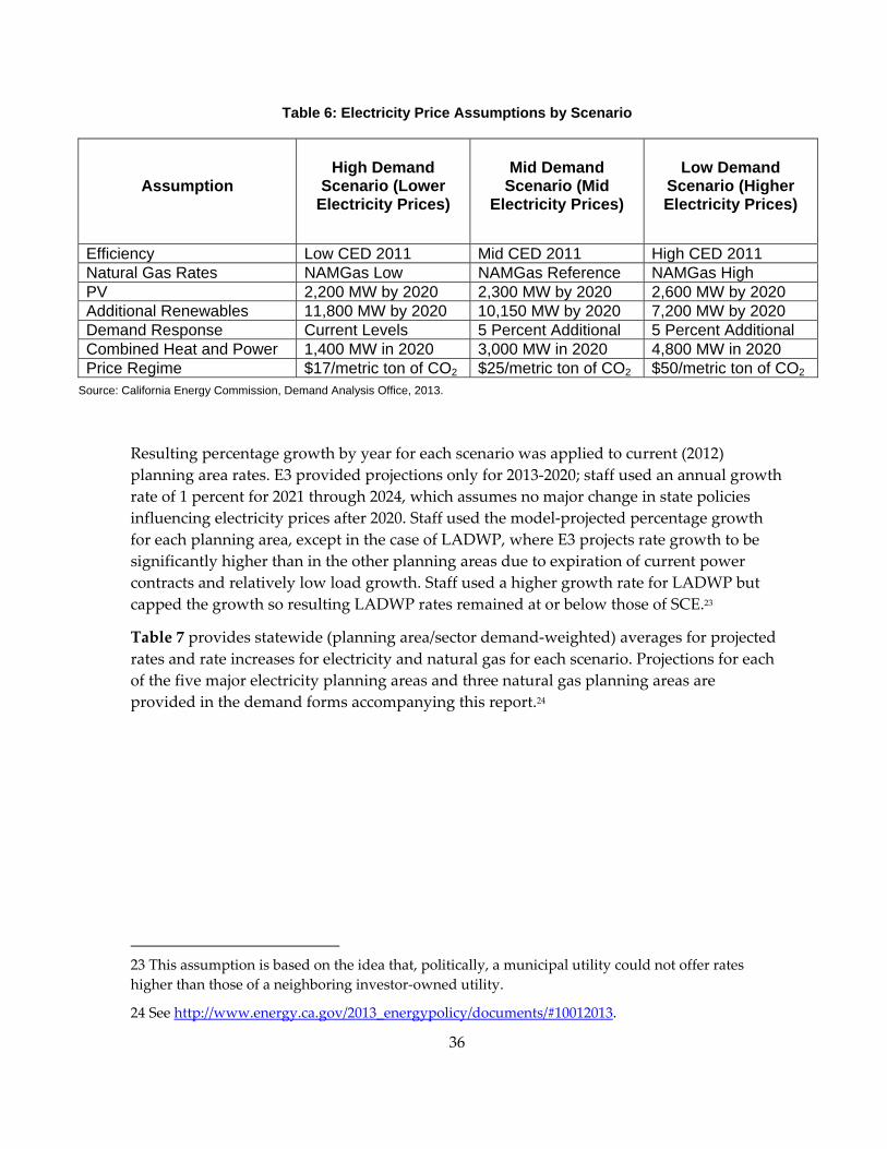
36

Table 6: Electricity Price Assumptions by Scenario

Assumption High Demand

Scenario (Lower Electricity Prices)

Mid Demand Scenario (Mid

Electricity Prices)

Low Demand Scenario (Higher Electricity Prices)

Efficiency Low CED 2011 Mid CED 2011 High CED 2011 Natural Gas Rates NAMGas Low NAMGas Reference NAMGas High PV 2,200 MW by 2020 2,300 MW by 2020 2,600 MW by 2020 Additional Renewables 11,800 MW by 2020 10,150 MW by 2020 7,200 MW by 2020 Demand Response Current Levels 5 Percent Additional 5 Percent Additional Combined Heat and Power 1,400 MW in 2020 3,000 MW in 2020 4,800 MW in 2020 Price Regime $17/metric ton of CO2 $25/metric ton of CO2 $50/metric ton of CO2


Resulting percentage growth by year for each scenario was applied to current (2012) planning area rates. E3 provided projections only for 2013‐2020; staff used an annual growth rate of 1 percent for 2021 through 2024, which assumes no major change in state policies influencing electricity prices after 2020. Staff used the model‐projected percentage growth for each planning area, except in the case of LADWP, where E3 projects rate growth to be significantly higher than in the other planning areas due to expiration of current power contracts and relatively low load growth. Staff used a higher growth rate for LADWP but capped the growth so resulting LADWP rates remained at or below those of SCE.23

Table 7 provides statewide (planning area/sector demand‐weighted) averages for projected rates and rate increases for electricity and natural gas for each scenario. Projections for each of the five major electricity planning areas and three natural gas planning areas are provided in the demand forms accompanying this report.24

23 This assumption is based on the idea that, politically, a municipal utility could not offer rates higher than those of a neighboring investor‐owned utility.

24 See http://www.energy.ca.gov/2013_energypolicy/documents/#10012013.

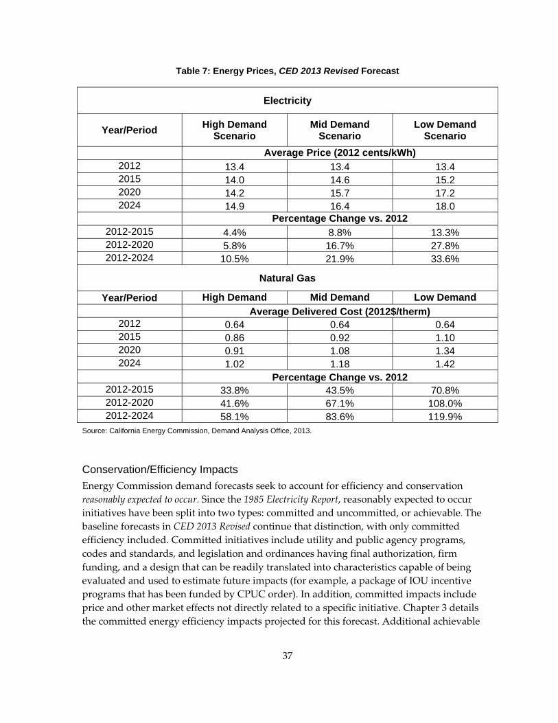
37

Table 7: Energy Prices, CED 2013 Revised Forecast

Electricity

Year/Period High Demand Scenario

Mid Demand Scenario

Low Demand Scenario

Average Price (2012 cents/kWh) 2012 13.4 13.4 13.4 2015 14.0 14.6 15.2 2020 14.2 15.7 17.2 2024 14.9 16.4 18.0

Percentage Change vs. 2012 2012-2015 4.4% 8.8% 13.3% 2012-2020 5.8% 16.7% 27.8% 2012-2024 10.5% 21.9% 33.6%

Natural Gas

Year/Period High Demand Mid Demand Low Demand Average Delivered Cost (2012$/therm)

2012 0.64 0.64 0.64 2015 0.86 0.92 1.10 2020 0.91 1.08 1.34 2024 1.02 1.18 1.42

Percentage Change vs. 2012 2012-2015 33.8% 43.5% 70.8% 2012-2020 41.6% 67.1% 108.0% 2012-2024 58.1% 83.6% 119.9%


Conservation/Efficiency Impacts Energy Commission demand forecasts seek to account for efficiency and conservation reasonably expected to occur. Since the 1985 Electricity Report, reasonably expected to occur initiatives have been split into two types: committed and uncommitted, or achievable. The baseline forecasts in CED 2013 Revised continue that distinction, with only committed efficiency included. Committed initiatives include utility and public agency programs, codes and standards, and legislation and ordinances having final authorization, firm funding, and a design that can be readily translated into characteristics capable of being evaluated and used to estimate future impacts (for example, a package of IOU incentive programs that has been funded by CPUC order). In addition, committed impacts include price and other market effects not directly related to a specific initiative. Chapter 3 details the committed energy efficiency impacts projected for this forecast. Additional achievable

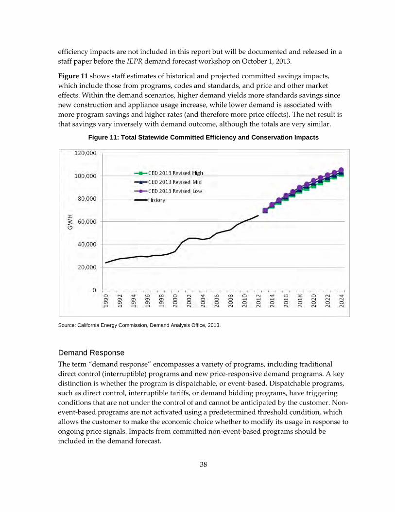
38

efficiency impacts are not included in this report but will be documented and released in a staff paper before the IEPR demand forecast workshop on October 1, 2013.

Figure 11 shows staff estimates of historical and projected committed savings impacts, which include those from programs, codes and standards, and price and other market effects. Within the demand scenarios, higher demand yields more standards savings since new construction and appliance usage increase, while lower demand is associated with more program savings and higher rates (and therefore more price effects). The net result is that savings vary inversely with demand outcome, although the totals are very similar.

Figure 11: Total Statewide Committed Efficiency and Conservation Impacts


Demand Response The term “demand response” encompasses a variety of programs, including traditional direct control (interruptible) programs and new price‐responsive demand programs. A key distinction is whether the program is dispatchable, or event‐based. Dispatchable programs, such as direct control, interruptible tariffs, or demand bidding programs, have triggering conditions that are not under the control of and cannot be anticipated by the customer. Non‐event‐based programs are not activated using a predetermined threshold condition, which allows the customer to make the economic choice whether to modify its usage in response to ongoing price signals. Impacts from committed non‐event‐based programs should be included in the demand forecast.

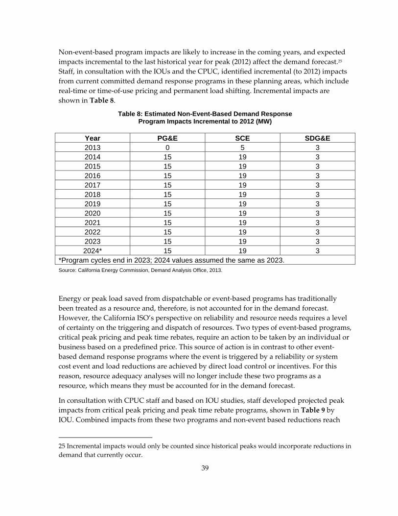
39

Non‐event‐based program impacts are likely to increase in the coming years, and expected impacts incremental to the last historical year for peak (2012) affect the demand forecast.25 Staff, in consultation with the IOUs and the CPUC, identified incremental (to 2012) impacts from current committed demand response programs in these planning areas, which include real‐time or time‐of‐use pricing and permanent load shifting. Incremental impacts are shown in Table 8.

Table 8: Estimated Non-Event-Based Demand Response Program Impacts Incremental to 2012 (MW)

Year PG&E SCE SDG&E 2013 0 5 3 2014 15 19 3 2015 15 19 3 2016 15 19 3 2017 15 19 3 2018 15 19 3 2019 15 19 3 2020 15 19 3 2021 15 19 3 2022 15 19 3 2023 15 19 3 2024* 15 19 3

*Program cycles end in 2023; 2024 values assumed the same as 2023. Source: California Energy Commission, Demand Analysis Office, 2013.

Energy or peak load saved from dispatchable or event‐based programs has traditionally been treated as a resource and, therefore, is not accounted for in the demand forecast. However, the California ISO’s perspective on reliability and resource needs requires a level of certainty on the triggering and dispatch of resources. Two types of event‐based programs, critical peak pricing and peak time rebates, require an action to be taken by an individual or business based on a predefined price. This source of action is in contrast to other event‐based demand response programs where the event is triggered by a reliability or system cost event and load reductions are achieved by direct load control or incentives. For this reason, resource adequacy analyses will no longer include these two programs as a resource, which means they must be accounted for in the demand forecast.

In consultation with CPUC staff and based on IOU studies, staff developed projected peak impacts from critical peak pricing and peak time rebate programs, shown in Table 9 by IOU. Combined impacts from these two programs and non‐event based reductions reach

25 Incremental impacts would only be counted since historical peaks would incorporate reductions in demand that currently occur.

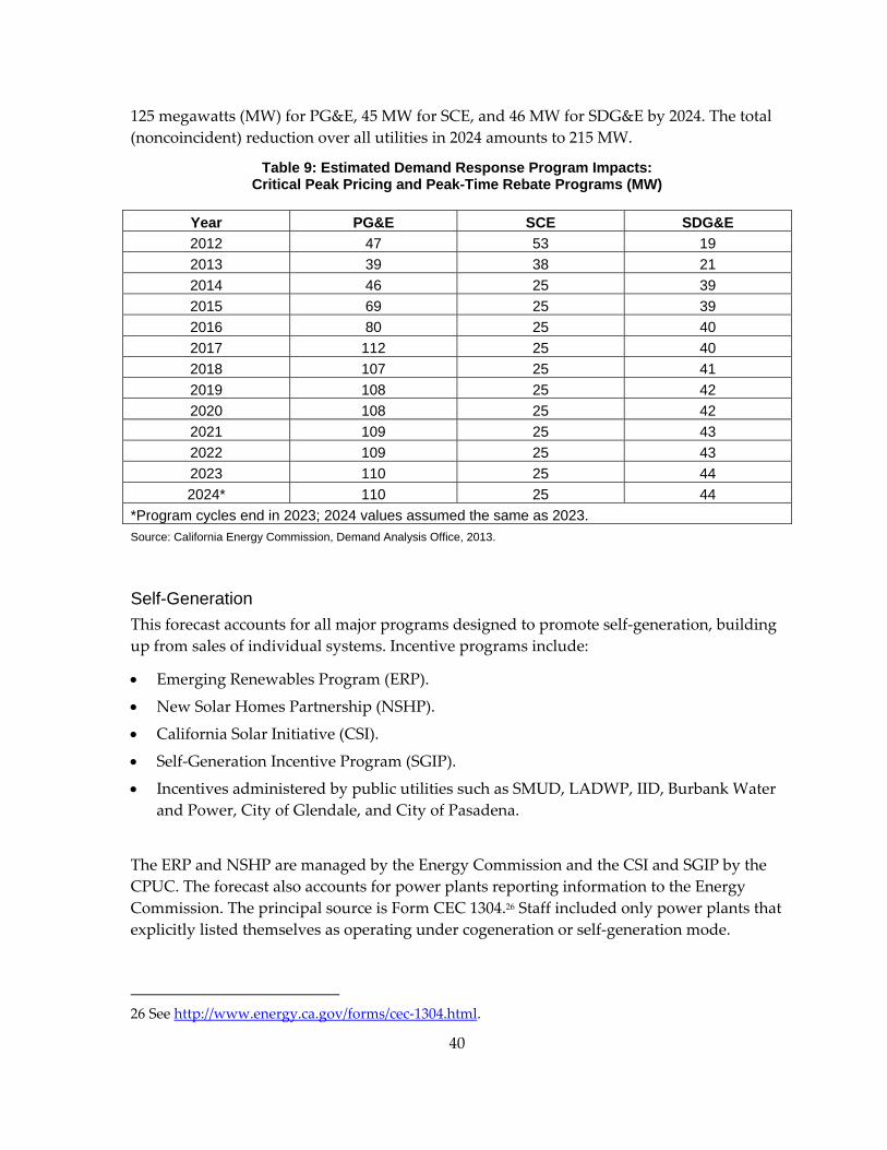
40

125 megawatts (MW) for PG&E, 45 MW for SCE, and 46 MW for SDG&E by 2024. The total (noncoincident) reduction over all utilities in 2024 amounts to 215 MW.

Table 9: Estimated Demand Response Program Impacts: Critical Peak Pricing and Peak-Time Rebate Programs (MW)

Year PG&E SCE SDG&E 2012 47 53 19 2013 39 38 21 2014 46 25 39 2015 69 25 39 2016 80 25 40 2017 112 25 40 2018 107 25 41 2019 108 25 42 2020 108 25 42 2021 109 25 43 2022 109 25 43 2023 110 25 44 2024* 110 25 44

*Program cycles end in 2023; 2024 values assumed the same as 2023. Source: California Energy Commission, Demand Analysis Office, 2013.

Self-Generation This forecast accounts for all major programs designed to promote self‐generation, building up from sales of individual systems. Incentive programs include:

• Emerging Renewables Program (ERP).

• New Solar Homes Partnership (NSHP).

• California Solar Initiative (CSI).

• Self‐Generation Incentive Program (SGIP).

• Incentives administered by public utilities such as SMUD, LADWP, IID, Burbank Water and Power, City of Glendale, and City of Pasadena.

The ERP and NSHP are managed by the Energy Commission and the CSI and SGIP by the CPUC. The forecast also accounts for power plants reporting information to the Energy Commission. The principal source is Form CEC 1304.26 Staff included only power plants that explicitly listed themselves as operating under cogeneration or self‐generation mode.

26 See http://www.energy.ca.gov/forms/cec‐1304.html.

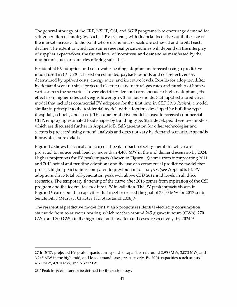
41

The general strategy of the ERP, NSHP, CSI, and SGIP programs is to encourage demand for self‐generation technologies, such as PV systems, with financial incentives until the size of the market increases to the point where economies of scale are achieved and capital costs decline. The extent to which consumers see real price declines will depend on the interplay of supplier expectations, the future level of incentives, and demand as manifested by the number of states or countries offering subsidies.

Residential PV adoption and solar water heating adoption are forecast using a predictive model used in CED 2011, based on estimated payback periods and cost‐effectiveness, determined by upfront costs, energy rates, and incentive levels. Results for adoption differ by demand scenario since projected electricity and natural gas rates and number of homes varies across the scenarios. Lower electricity demand corresponds to higher adoptions; the effect from higher rates outweighs lower growth in households. Staff applied a predictive model that includes commercial PV adoption for the first time in CED 2013 Revised, a model similar in principle to the residential model, with adoptions developed by building type (hospitals, schools, and so on). The same predictive model is used to forecast commercial CHP, employing estimated load shapes by building type. Staff developed these two models, which are discussed further in Appendix B. Self‐generation for other technologies and sectors is projected using a trend analysis and does not vary by demand scenario. Appendix B provides more details.

Figure 12 shows historical and projected peak impacts of self‐generation, which are projected to reduce peak load by more than 4,400 MW in the mid demand scenario by 2024. Higher projections for PV peak impacts (shown in Figure 13) come from incorporating 2011 and 2012 actual and pending adoptions and the use of a commercial predictive model that projects higher penetrations compared to previous trend analyses (see Appendix B). PV adoptions drive total self‐generation peak well above CED 2011 mid levels in all three scenarios. The temporary flattening of the curve after 2016 comes from expiration of the CSI program and the federal tax credit for PV installation. The PV peak impacts shown in Figure 13 correspond to capacities that meet or exceed the goal of 3,000 MW for 2017 set in Senate Bill 1 (Murray, Chapter 132, Statutes of 2006).27

The residential predictive model for PV also projects residential electricity consumption statewide from solar water heating, which reaches around 245 gigawatt hours (GWh), 270 GWh, and 300 GWh in the high, mid, and low demand cases, respectively, by 2024.28

27 In 2017, projected PV peak impacts correspond to capacities of around 2,950 MW, 3,070 MW, and 3,245 MW in the high, mid, and low demand cases, respectively. By 2024, capacities reach around 4,370MW, 4,970 MW, and 5,690 MW.

28 “Peak impacts” cannot be defined for this technology.

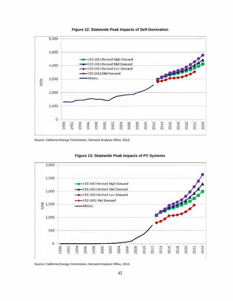
42

Figure 12: Statewide Peak Impacts of Self-Generation


Figure 13: Statewide Peak Impacts of PV Systems


43

Table 10 shows historical and projected statewide electricity consumption from self‐generation, broken out into PV and non‐PV applications. For traditional industrial CHP technologies, self‐generation is assumed constant (no clear trend is evident in the historical data), so that retired CHP plants are replaced with new ones with no net change in generation. Growth in non‐PV self‐generation comes mainly from recent increases in the application of fuel cells projected forward and from commercial CHP.

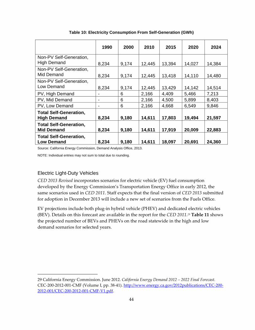
44

Table 10: Electricity Consumption From Self-Generation (GWh)

1990 2000 2010 2015 2020 2024

Non-PV Self-Generation, High Demand 8,234 9,174 12,445 13,394 14,027 14,384 Non-PV Self-Generation, Mid Demand 8,234 9,174 12,445 13,418 14,110 14,480 Non-PV Self-Generation, Low Demand 8,234 9,174 12,445 13,429 14,142 14,514 PV, High Demand - 6 2,166 4,409 5,466 7,213 PV, Mid Demand - 6 2,166 4,500 5,899 8,403 PV, Low Demand - 6 2,166 4,668 6,549 9,846 Total Self-Generation, High Demand 8,234 9,180 14,611 17,803 19,494 21,597 Total Self-Generation, Mid Demand 8,234 9,180 14,611 17,919 20,009 22,883 Total Self-Generation, Low Demand 8,234 9,180 14,611 18,097 20,691 24,360 Source: California Energy Commission, Demand Analysis Office, 2013.

NOTE: Individual entries may not sum to total due to rounding.

Electric Light-Duty Vehicles CED 2013 Revised incorporates scenarios for electric vehicle (EV) fuel consumption developed by the Energy Commission’s Transportation Energy Office in early 2012, the same scenarios used in CED 2011. Staff expects that the final version of CED 2013 submitted for adoption in December 2013 will include a new set of scenarios from the Fuels Office.

EV projections include both plug‐in hybrid vehicle (PHEV) and dedicated electric vehicles (BEV). Details on this forecast are available in the report for the CED 2011.29 Table 11 shows the projected number of BEVs and PHEVs on the road statewide in the high and low demand scenarios for selected years.

29 California Energy Commission. June 2012. California Energy Demand 2012 – 2022 Final Forecast. CEC‐200‐2012‐001‐CMF (Volume I, pp. 38‐41). http://www.energy.ca.gov/2012publications/CEC‐200‐2012‐001/CEC‐200‐2012‐001‐CMF‐V1.pdf.

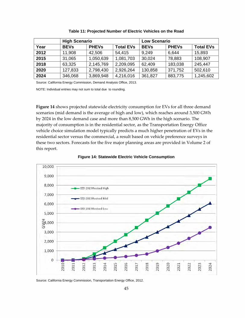
45

Table 11: Projected Number of Electric Vehicles on the Road

High Scenario Low Scenario Year BEVs PHEVs Total EVs BEVs PHEVs Total EVs 2012 11,908 42,506 54,415 9,249 6,644 15,893 2015 31,065 1,050,639 1,081,703 30,024 78,883 108,907 2018 63,325 2,145,769 2,209,095 62,409 183,038 245,447 2020 127,833 2,798,430 2,926,264 130,858 371,752 502,610 2024 346,068 3,869,948 4,216,016 361,827 883,775 1,245,602 Source: California Energy Commission, Demand Analysis Office, 2013.


Figure 14 shows projected statewide electricity consumption for EVs for all three demand scenarios (mid demand is the average of high and low), which reaches around 3,500 GWh by 2024 in the low demand case and more than 8,500 GWh in the high scenario. The majority of consumption is in the residential sector, as the Transportation Energy Office vehicle choice simulation model typically predicts a much higher penetration of EVs in the residential sector versus the commercial, a result based on vehicle preference surveys in these two sectors. Forecasts for the five major planning areas are provided in Volume 2 of this report.

Figure 14: Statewide Electric Vehicle Consumption

Source: California Energy Commission, Transportation Energy Office, 2012.

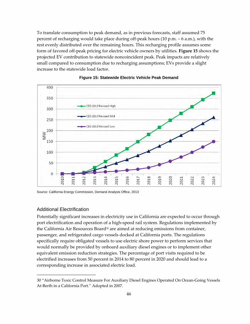
46

To translate consumption to peak demand, as in previous forecasts, staff assumed 75 percent of recharging would take place during off‐peak hours (10 p.m. – 6 a.m.), with the rest evenly distributed over the remaining hours. This recharging profile assumes some form of favored off‐peak pricing for electric vehicle owners by utilities. Figure 15 shows the projected EV contribution to statewide noncoincident peak. Peak impacts are relatively small compared to consumption due to recharging assumptions; EVs provide a slight increase to the statewide load factor.

Figure 15: Statewide Electric Vehicle Peak Demand

Source: California Energy Commission, Demand Analysis Office, 2013

Additional Electrification Potentially significant increases in electricity use in California are expected to occur through port electrification and operation of a high‐speed rail system. Regulations implemented by the California Air Resources Board30 are aimed at reducing emissions from container, passenger, and refrigerated cargo vessels docked at California ports. The regulations specifically require obligated vessels to use electric shore power to perform services that would normally be provided by onboard auxiliary diesel engines or to implement other equivalent emission reduction strategies. The percentage of port visits required to be electrified increases from 50 percent in 2014 to 80 percent in 2020 and should lead to a corresponding increase in associated electric load.

30 “Airborne Toxic Control Measure For Auxiliary Diesel Engines Operated On Ocean‐Going Vessels At‐Berth in a California Port.” Adopted in 2007.

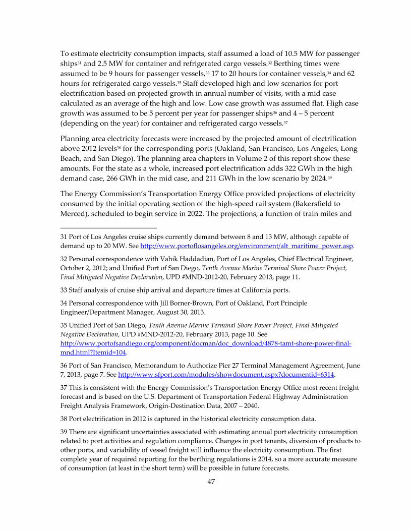
47

To estimate electricity consumption impacts, staff assumed a load of 10.5 MW for passenger ships31 and 2.5 MW for container and refrigerated cargo vessels.32 Berthing times were assumed to be 9 hours for passenger vessels,33 17 to 20 hours for container vessels,34 and 62 hours for refrigerated cargo vessels.35 Staff developed high and low scenarios for port electrification based on projected growth in annual number of visits, with a mid case calculated as an average of the high and low. Low case growth was assumed flat. High case growth was assumed to be 5 percent per year for passenger ships36 and 4 – 5 percent (depending on the year) for container and refrigerated cargo vessels.37

Planning area electricity forecasts were increased by the projected amount of electrification above 2012 levels38 for the corresponding ports (Oakland, San Francisco, Los Angeles, Long Beach, and San Diego). The planning area chapters in Volume 2 of this report show these amounts. For the state as a whole, increased port electrification adds 322 GWh in the high demand case, 266 GWh in the mid case, and 211 GWh in the low scenario by 2024.39

The Energy Commission’s Transportation Energy Office provided projections of electricity consumed by the initial operating section of the high‐speed rail system (Bakersfield to Merced), scheduled to begin service in 2022. The projections, a function of train miles and

31 Port of Los Angeles cruise ships currently demand between 8 and 13 MW, although capable of demand up to 20 MW. See http://www.portoflosangeles.org/environment/alt_maritime_power.asp.

32 Personal correspondence with Vahik Haddadian, Port of Los Angeles, Chief Electrical Engineer, October 2, 2012; and Unified Port of San Diego, Tenth Avenue Marine Terminal Shore Power Project, Final Mitigated Negative Declaration, UPD #MND‐2012‐20, February 2013, page 11.

33 Staff analysis of cruise ship arrival and departure times at California ports.

34 Personal correspondence with Jill Borner‐Brown, Port of Oakland, Port Principle Engineer/Department Manager, August 30, 2013.

35 Unified Port of San Diego, Tenth Avenue Marine Terminal Shore Power Project, Final Mitigated Negative Declaration, UPD #MND‐2012‐20, February 2013, page 10. See http://www.portofsandiego.org/component/docman/doc_download/4878‐tamt‐shore‐power‐final‐mnd.html?Itemid=104.

36 Port of San Francisco, Memorandum to Authorize Pier 27 Terminal Management Agreement, June 7, 2013, page 7. See http://www.sfport.com/modules/showdocument.aspx?documentid=6314.

37 This is consistent with the Energy Commission’s Transportation Energy Office most recent freight forecast and is based on the U.S. Department of Transportation Federal Highway Administration Freight Analysis Framework, Origin‐Destination Data, 2007 – 2040.

38 Port electrification in 2012 is captured in the historical electricity consumption data.

39 There are significant uncertainties associated with estimating annual port electricity consumption related to port activities and regulation compliance. Changes in port tenants, diversion of products to other ports, and variability of vessel freight will influence the electricity consumption. The first complete year of required reporting for the berthing regulations is 2014, so a more accurate measure of consumption (at least in the short term) will be possible in future forecasts.

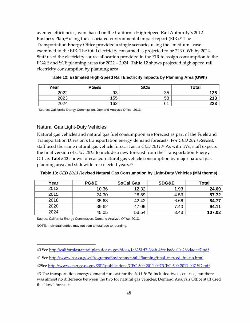
48

average efficiencies, were based on the California High‐Speed Rail Authority’s 2012 Business Plan,40 using the associated environmental impact report (EIR).41 The Transportation Energy Office provided a single scenario, using the “medium” case examined in the EIR. The total electricity consumed is projected to be 223 GWh by 2024. Staff used the electricity source allocation provided in the EIR to assign consumption to the PG&E and SCE planning areas for 2022 – 2024. Table 12 shows projected high‐speed rail electricity consumption by planning area.

Table 12: Estimated High-Speed Rail Electricity Impacts by Planning Area (GWh)

Year PG&E SCE Total 2022 93 35 1282023 155 58 2132024 162 61 223


Natural Gas Light-Duty Vehicles Natural gas vehicles and natural gas fuel consumption are forecast as part of the Fuels and Transportation Division’s transportation energy demand forecasts. For CED 2013 Revised, staff used the same natural gas vehicle forecast as in CED 2011.42 As with EVs, staff expects the final version of CED 2013 to include a new forecast from the Transportation Energy Office. Table 13 shows forecasted natural gas vehicle consumption by major natural gas planning area and statewide for selected years.43

Table 13: CED 2013 Revised Natural Gas Consumption by Light-Duty Vehicles (MM therms)

Year PG&E SoCal Gas SDG&E Total 2012 10.36 12.32 1.93 24.602015 24.30 28.89 4.53 57.722018 35.68 42.42 6.66 84.772020 39.62 47.09 7.40 94.112024 45.05 53.54 8.43 107.02



40 See http://californiastaterailplan.dot.ca.gov/docs/1a6251d7‐36ab‐4fec‐ba8c‐00e266dadec7.pdf.

41 See http://www.hsr.ca.gov/Programs/Environmental_Planning/final_merced_fresno.html.

42See http://www.energy.ca.gov/2011publications/CEC‐600‐2011‐007/CEC‐600‐2011‐007‐SD.pdf.

43 The transportation energy demand forecast for the 2011 IEPR included two scenarios, but there was almost no difference between the two for natural gas vehicles; Demand Analysis Office staff used the “low” forecast.

49

Subregional Electricity Analysis As discussed earlier in this chapter, staff intends to provide, to the extent possible, more granular results in future demand forecasts. An important reason is to support subregional electricity system analysis for CPUC/California ISO resource adequacy and other related proceedings. Staff currently disaggregates, or separates, the planning area and climate zone forecasts to correspond to control areas and congestion zones in a “top down” analysis. Further disaggregation of the demand forecast (beyond the climate zone level) would allow more refined, “bottom up” analyses for local congestion zones.

Subregional forecasts for both energy and peak demand are provided in spreadsheet files (Form 1.5) in the forms accompanying this forecast report.44 To develop subregional peak demand forecasts, staff estimates weather‐normalized peaks for the IOU transmission access charge (TAC) areas, as well as PG&E Bay and non‐Bay subareas, using regression analysis and the latest hourly load data available.45 The regression results provide weather sensitivity for a reference year (in this case, 2012) so that peak demand can be normalized, assuming average weather (“1 in 2”) and extreme weather (“1 in 10”) using 30 – 60 years of temperature data. Weather‐normalized peaks are then projected in a manner consistent with the demand forecasts for the appropriate planning area.46 Local area peaks within IOU TAC areas are estimated using the latest load data available and “trued up” (brought into alignment) to IOU TAC totals. More details about these methods are available in a 2011 Energy Commission Committee report.47

Historical Electricity Consumption Estimates Energy Commission demand forecasting models are organized by sector according to economic activity (that is, commercial, industrial, agricultural, and so on). Each model develops a forecast based on subactivities within the sector (for example, commercial building type or industrial activity). Under the Energy Commission’s Quarterly Fuel and

44 See http://www.energy.ca.gov/2013_energypolicy/documents/2013‐10‐01_workshop/spreadsheets/.

45 The TAC areas include the IOUs and, for Pacific Gas and Electric and Southern California Edison, publicly owned utilities utilizing the IOU’s transmission system.

46 For example, the PG&E TAC area peak demand is assumed to grow at the projected rate of the PG&E planning area.

47 Garcia‐Cerrutti, Miguel, Tom Gorin, Chris Kavalec, Lynn Marshall. 2011. Final Short‐Term (2011 – 2012) Peak Demand Forecast Committee Final Report. California Energy Commission, Electricity Supply Analysis Division. Available at http://www.energy.ca.gov/2011publications/CEC‐200‐2011‐002/CEC‐200‐2011‐002‐CTF.pdf.

50

Energy Report (QFER) regulations, each load‐serving entity (LSE) is required to file quarterly reports documenting energy consumption by activity group.

The quality of the QFER data is improving but is still occasionally undermined by LSE data coding errors, lack of adherence to regulations, and failure to provide economic classification for some of the data. Unclassified consumption, after declining from a high of almost 20,000 GWh in 2003 to less than 6,000 GWh in 2010, has increased to 10,000 GWh in 2012. Staff allocates unclassified consumption to economic sectors using professional judgment, relying on factors such as unrealistic changes in historical consumption.

Staff is developing a database system to automate QFER data collection and processing, which should promote more accurate LSE filings. A test version of this database is scheduled to be complete by the end of 2013.

Structure of Report

Chapter 2 of Volume 1 provides statewide results for the end‐user natural gas forecast, along with results for the PG&E, SoCal Gas, and SDG&E distribution areas. Chapter 3 presents committed energy efficiency and conservation savings estimated for the forecast. The appendices provide additional information about methods and econometric results, incorporation of climate change, self‐generation, and regression results.

Volume 2 provides CED 2013 Revised electricity forecasts for the following planning areas: PG&E, SCE, SDG&E, SMUD, and LADWP. The planning areas included in this forecast are described in Table 14. The chapters for LADWP, PG&E, and SCE in Volume 2 provide results for the climate zones within these planning areas. Figure 16 shows the Energy Commission’s forecasting climate zones. Zones 1 − 5 correspond to PG&E, 7 – 10 to SCE, and 11 – 12 to LADWP. The other planning areas correspond to single climate zones. The areas labeled “Other” correspond to areas in California served (for electricity) by out‐of‐state entities and not included in the eight planning areas. Forecast demand forms for each planning area are posted with this report. 48

48 See http://energy.ca.gov/2013_energypolicy/documents/#10012013.

51

Table 14: Utilities Within Forecasting Areas

Planning Area Utilities Included Electric Areas

PG&E

PG&E Alameda Biggs Calaveras Gridley Healdsburg Hercules Island Energy (Pittsburg) Lassen Lodi Lompoc Merced Modesto Palo Alto

Plumas – Sierra Port of Oakland Port of Stockton Power and Water Resources Pooling Authority Redding Roseville San Francisco Shasta Silicon Valley Tuolumne Turlock Irrigation District Ukiah U.S. Bureau of Reclamation-Central Valley Project

SMUD SMUD

SCE

Anaheim Anza Azusa Banning Bear Valley Colton Corona Metropolitan Water District

Moreno Valley Rancho Cucamonga Riverside SCE U.S. Bureau of Reclamation-Parker Davis Valley Electric Vernon Victorville

LADWP LADWP SDG&E SDG&E Cities of Burbank and Glendale (BUGL) Burbank, Glendale Pasadena (PASD) Pasadena Imperial (IID) Imperial Irrigation District Department of Water Resources (DWR) DWR Natural Gas Distribution Areas PG&E PG&E, Palo Alto SDG&E SDG&E

SoCal Gas SoCal Gas, Long Beach, Northwest Pipeline, Mojave Pipeline

OTHER Southwest Gas Corporation, Avista Energy Source: California Energy Commission, Demand Analysis Office, 2013.

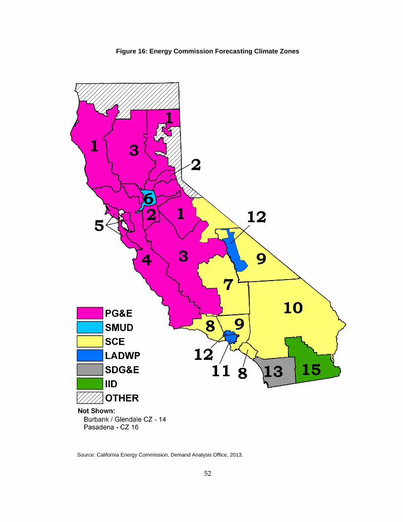
52

Figure 16: Energy Commission Forecasting Climate Zones


53

CHAPTER 2: End-User Natural Gas Demand Forecast This chapter presents revised baseline forecasts of end‐user natural gas demand for the PG&E, SoCal Gas, and SDG&E natural gas planning areas. In addition, statewide results include sales from smaller utilities, including Southwest Gas Corporation, aggregated into the category “other.” Detailed forecasts for the three major planning areas and “other” are provided in the electronic natural gas forms accompanying this forecast report.49

Staff prepares these forecasts in parallel with its electricity demand forecasts, with the same models, organized along electricity planning area boundaries. The gas demand forecasts presented here are the combination of gas demand in the corresponding electricity planning areas. These forecasts do not include natural gas used by utilities or others for electric generation but include projections for light‐duty natural gas vehicle fuel use, as discussed in Chapter 1 of this volume.

CED 2013 Revised incorporates historical natural gas consumption data up through 2012. Three demand scenarios were forecast (high, mid, and low), with the same economic/demographic assumptions as used for electricity. Also similar to electricity, the high, mid, and low scenarios incorporated low, mid, and high assumptions, respectively, for natural gas prices and committed efficiency program impacts. See Chapter 1 for a discussion of prices and economic and demographic inputs and Chapter 3 for a description of committed efficiency assumptions. Finally, statewide and major planning area results are shown with and without estimates of incremental achievable efficiency, referred to as baseline and adjusted forecasts, respectively. Incremental achievable efficiency is described further in Chapter 3.

Statewide Baseline Forecast Results

Table 15 compares the three CED 2013 Revised baseline demand scenarios at the statewide level with the CED 2011 mid demand case for selected years. The new forecasts begin at a lower point in 2012, as natural gas consumption in California was substantially lower this year than was predicted in the CED 2011 mid case, and grow at a slower rate in all three scenarios from 2012 – 2022. Key factors are slower projected population growth in the CED 2013 Revised mid and low cases, the introduction of climate change impacts in the mid and high cases,50 and new efficiency initiatives and higher projected natural gas rates for all three scenarios. Climate change affects the mid and high scenarios through projected

49 See http://energy.ca.gov/2013_energypolicy/documents/#10012013.

50 Potential climate change impacts on end‐user natural gas consumption were not estimated for CED 2011.

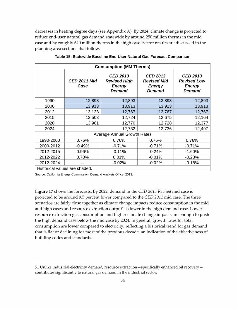
54

decreases in heating degree days (see Appendix A). By 2024, climate change is projected to reduce end‐user natural gas demand statewide by around 250 million therms in the mid case and by roughly 640 million therms in the high case. Sector results are discussed in the planning area sections that follow.

Table 15: Statewide Baseline End-User Natural Gas Forecast Comparison


CED 2011 Mid Case


Energy Demand


Energy Demand


Energy Demand

1990 12,893 12,893 12,893 12,8932000 13,913 13,913 13,913 13,9132012 13,123 12,767 12,767 12,7672015 13,503 12,724 12,675 12,1642020 13,961 12,770 12,728 12,3772024 -- 12,732 12,736 12,497



Figure 17 shows the forecasts. By 2022, demand in the CED 2013 Revised mid case is projected to be around 9.5 percent lower compared to the CED 2011 mid case. The three scenarios are fairly close together as climate change impacts reduce consumption in the mid and high cases and resource extraction output51 is lower in the high demand case. Lower resource extraction gas consumption and higher climate change impacts are enough to push the high demand case below the mid case by 2024. In general, growth rates for total consumption are lower compared to electricity, reflecting a historical trend for gas demand that is flat or declining for most of the previous decade, an indication of the effectiveness of building codes and standards.

51 Unlike industrial electricity demand, resource extraction—specifically enhanced oil recovery—contributes significantly to natural gas demand in the industrial sector.

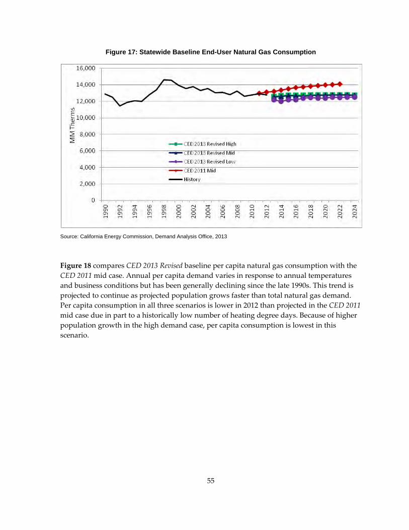
55

Figure 17: Statewide Baseline End-User Natural Gas Consumption


Figure 18 compares CED 2013 Revised baseline per capita natural gas consumption with the CED 2011 mid case. Annual per capita demand varies in response to annual temperatures and business conditions but has been generally declining since the late 1990s. This trend is projected to continue as projected population grows faster than total natural gas demand. Per capita consumption in all three scenarios is lower in 2012 than projected in the CED 2011 mid case due in part to a historically low number of heating degree days. Because of higher population growth in the high demand case, per capita consumption is lowest in this scenario.

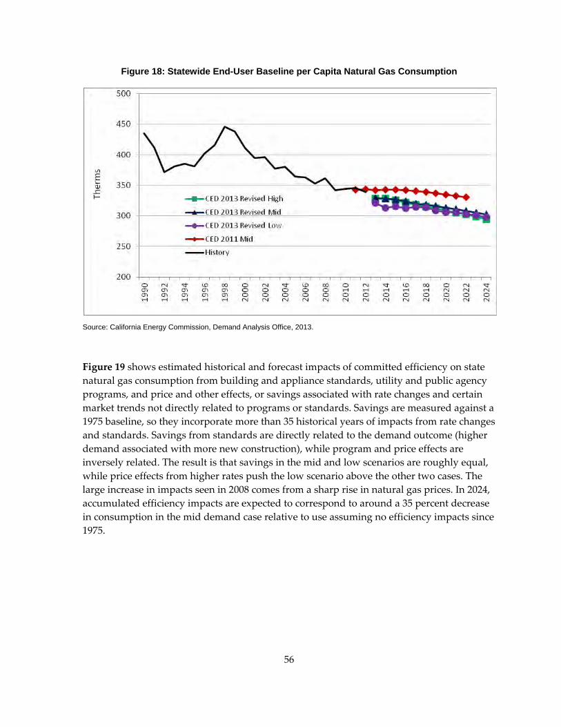
56

Figure 18: Statewide End-User Baseline per Capita Natural Gas Consumption


Figure 19 shows estimated historical and forecast impacts of committed efficiency on state natural gas consumption from building and appliance standards, utility and public agency programs, and price and other effects, or savings associated with rate changes and certain market trends not directly related to programs or standards. Savings are measured against a 1975 baseline, so they incorporate more than 35 historical years of impacts from rate changes and standards. Savings from standards are directly related to the demand outcome (higher demand associated with more new construction), while program and price effects are inversely related. The result is that savings in the mid and low scenarios are roughly equal, while price effects from higher rates push the low scenario above the other two cases. The large increase in impacts seen in 2008 comes from a sharp rise in natural gas prices. In 2024, accumulated efficiency impacts are expected to correspond to around a 35 percent decrease in consumption in the mid demand case relative to use assuming no efficiency impacts since 1975.

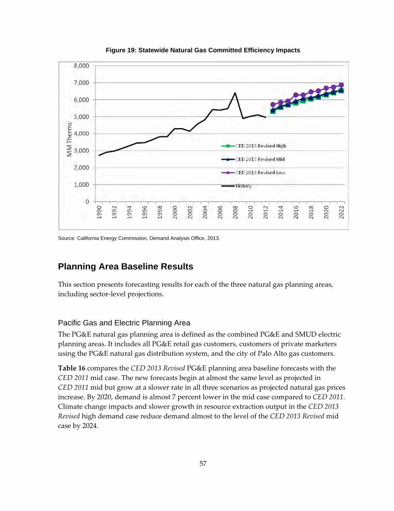
57

Figure 19: Statewide Natural Gas Committed Efficiency Impacts


Planning Area Baseline Results

This section presents forecasting results for each of the three natural gas planning areas, including sector‐level projections.

Pacific Gas and Electric Planning Area The PG&E natural gas planning area is defined as the combined PG&E and SMUD electric planning areas. It includes all PG&E retail gas customers, customers of private marketers using the PG&E natural gas distribution system, and the city of Palo Alto gas customers.

Table 16 compares the CED 2013 Revised PG&E planning area baseline forecasts with the CED 2011 mid case. The new forecasts begin at almost the same level as projected in CED 2011 mid but grow at a slower rate in all three scenarios as projected natural gas prices increase. By 2020, demand is almost 7 percent lower in the mid case compared to CED 2011. Climate change impacts and slower growth in resource extraction output in the CED 2013 Revised high demand case reduce demand almost to the level of the CED 2013 Revised mid case by 2024.

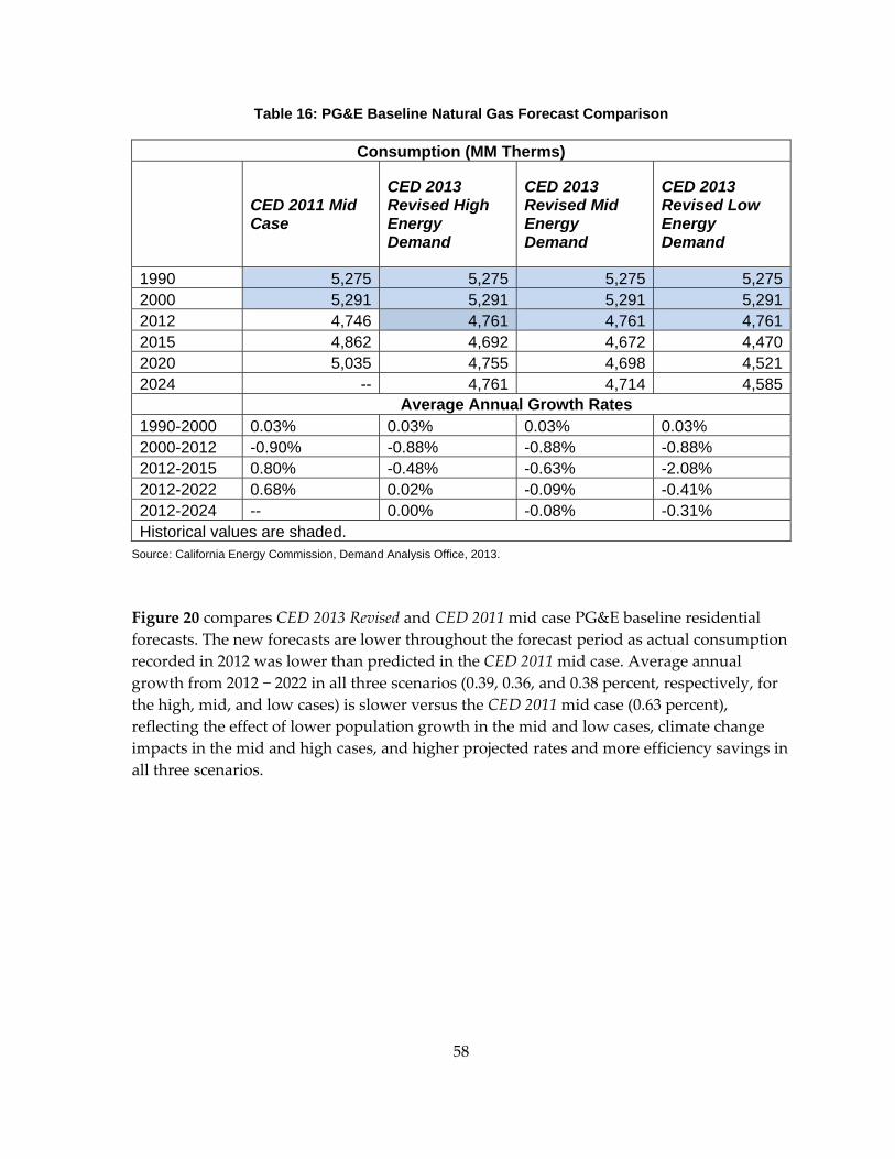
58

Table 16: PG&E Baseline Natural Gas Forecast Comparison


CED 2011 Mid Case

CED 2013 Revised High Energy Demand

CED 2013 Revised Mid Energy Demand

CED 2013 Revised Low Energy Demand

1990 5,275 5,275 5,275 5,2752000 5,291 5,291 5,291 5,2912012 4,746 4,761 4,761 4,7612015 4,862 4,692 4,672 4,4702020 5,035 4,755 4,698 4,5212024 -- 4,761 4,714 4,585 Average Annual Growth Rates 1990-2000 0.03% 0.03% 0.03% 0.03% 2000-2012 -0.90% -0.88% -0.88% -0.88% 2012-2015 0.80% -0.48% -0.63% -2.08% 2012-2022 0.68% 0.02% -0.09% -0.41% 2012-2024 -- 0.00% -0.08% -0.31% Historical values are shaded.


Figure 20 compares CED 2013 Revised and CED 2011 mid case PG&E baseline residential forecasts. The new forecasts are lower throughout the forecast period as actual consumption recorded in 2012 was lower than predicted in the CED 2011 mid case. Average annual growth from 2012 − 2022 in all three scenarios (0.39, 0.36, and 0.38 percent, respectively, for the high, mid, and low cases) is slower versus the CED 2011 mid case (0.63 percent), reflecting the effect of lower population growth in the mid and low cases, climate change impacts in the mid and high cases, and higher projected rates and more efficiency savings in all three scenarios.

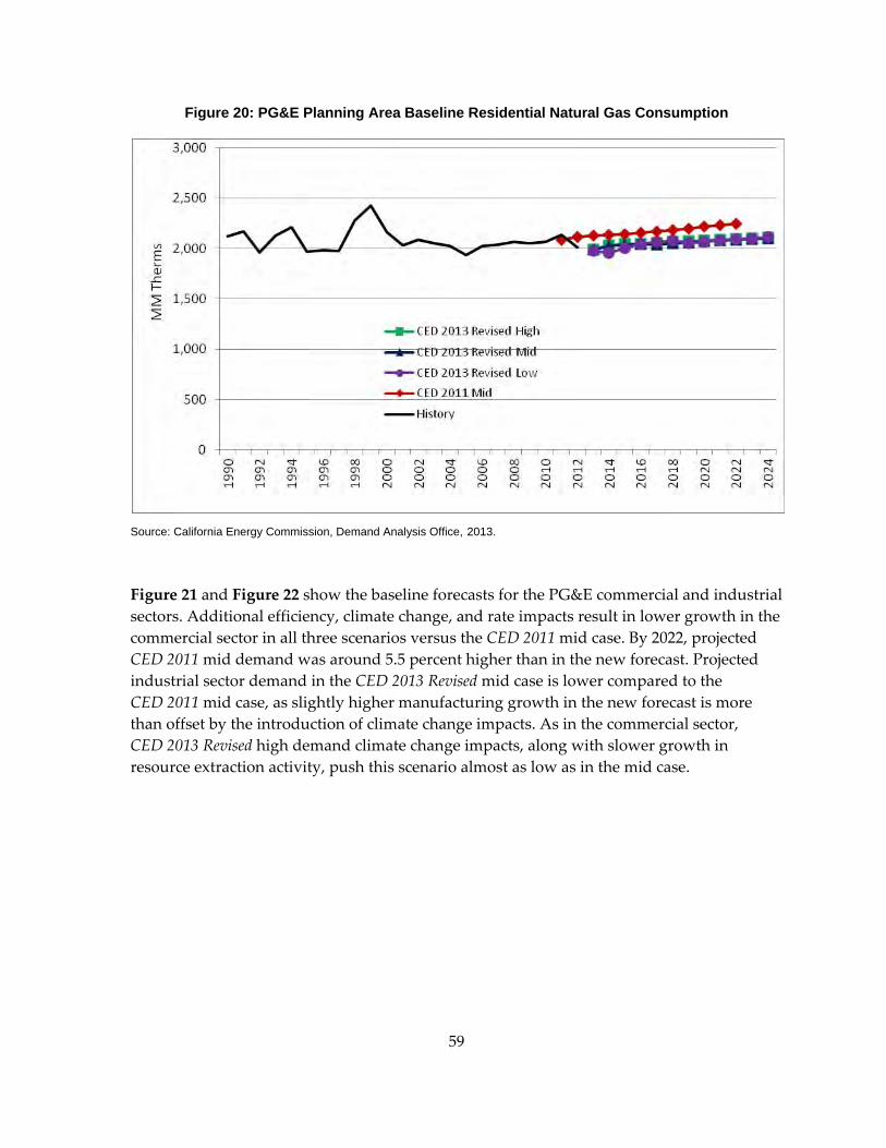
59

Figure 20: PG&E Planning Area Baseline Residential Natural Gas Consumption


Figure 21 and Figure 22 show the baseline forecasts for the PG&E commercial and industrial sectors. Additional efficiency, climate change, and rate impacts result in lower growth in the commercial sector in all three scenarios versus the CED 2011 mid case. By 2022, projected CED 2011 mid demand was around 5.5 percent higher than in the new forecast. Projected industrial sector demand in the CED 2013 Revised mid case is lower compared to the CED 2011 mid case, as slightly higher manufacturing growth in the new forecast is more than offset by the introduction of climate change impacts. As in the commercial sector, CED 2013 Revised high demand climate change impacts, along with slower growth in resource extraction activity, push this scenario almost as low as in the mid case.

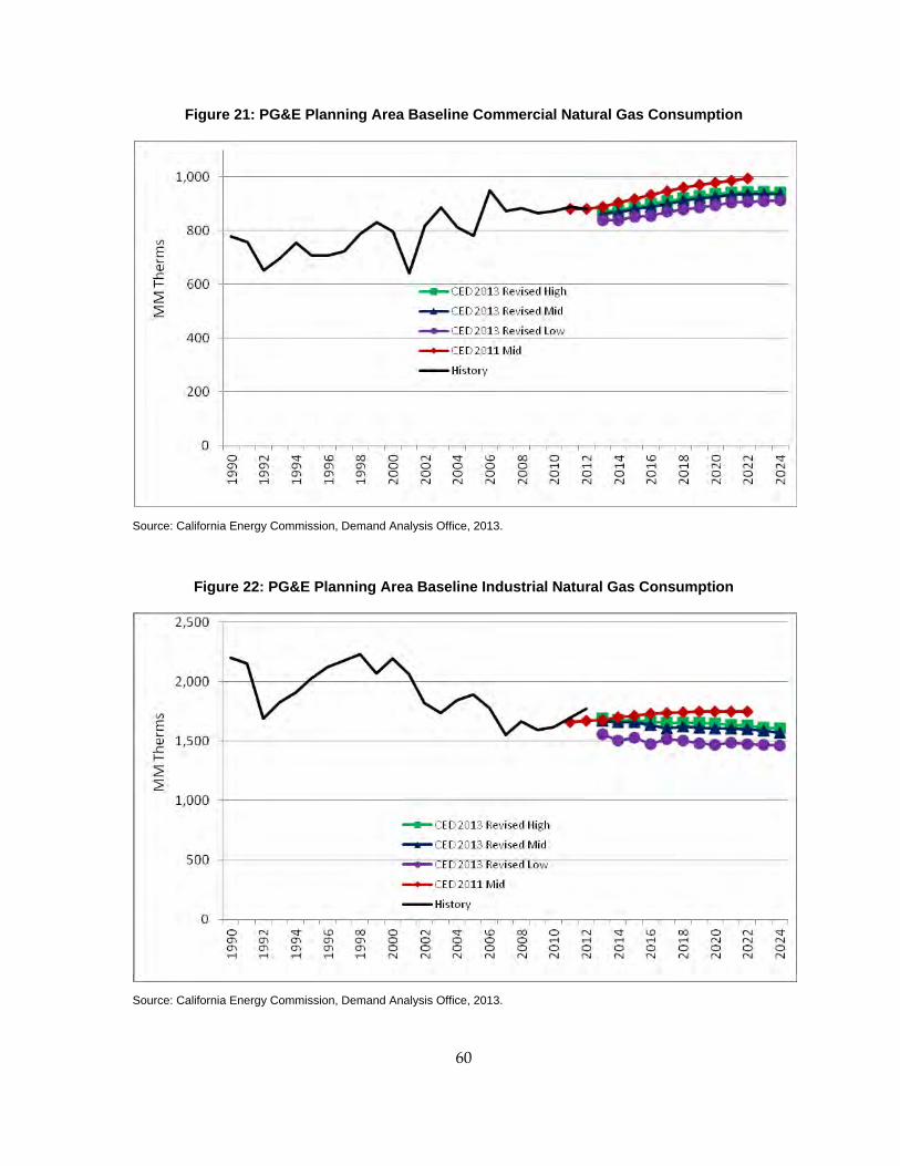
60

Figure 21: PG&E Planning Area Baseline Commercial Natural Gas Consumption


Figure 22: PG&E Planning Area Baseline Industrial Natural Gas Consumption


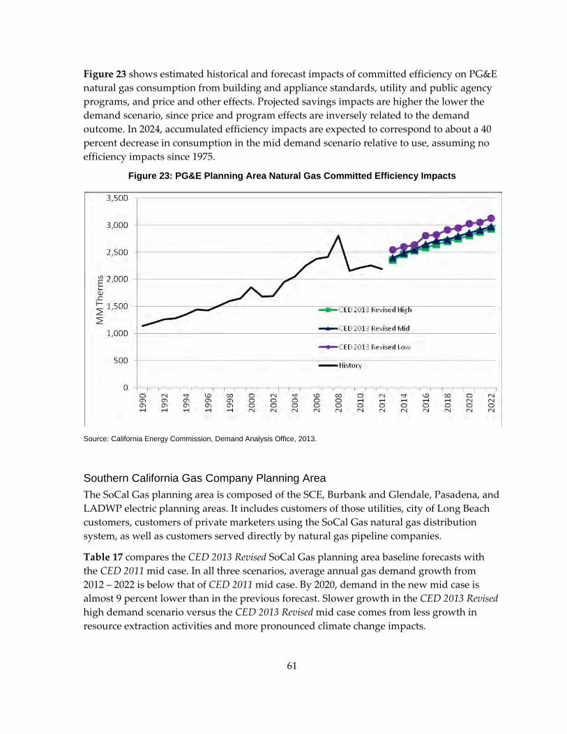
61

Figure 23 shows estimated historical and forecast impacts of committed efficiency on PG&E natural gas consumption from building and appliance standards, utility and public agency programs, and price and other effects. Projected savings impacts are higher the lower the demand scenario, since price and program effects are inversely related to the demand outcome. In 2024, accumulated efficiency impacts are expected to correspond to about a 40 percent decrease in consumption in the mid demand scenario relative to use, assuming no efficiency impacts since 1975.

Figure 23: PG&E Planning Area Natural Gas Committed Efficiency Impacts


Southern California Gas Company Planning Area The SoCal Gas planning area is composed of the SCE, Burbank and Glendale, Pasadena, and LADWP electric planning areas. It includes customers of those utilities, city of Long Beach customers, customers of private marketers using the SoCal Gas natural gas distribution system, as well as customers served directly by natural gas pipeline companies.

Table 17 compares the CED 2013 Revised SoCal Gas planning area baseline forecasts with the CED 2011 mid case. In all three scenarios, average annual gas demand growth from 2012 – 2022 is below that of CED 2011 mid case. By 2020, demand in the new mid case is almost 9 percent lower than in the previous forecast. Slower growth in the CED 2013 Revised high demand scenario versus the CED 2013 Revised mid case comes from less growth in resource extraction activities and more pronounced climate change impacts.

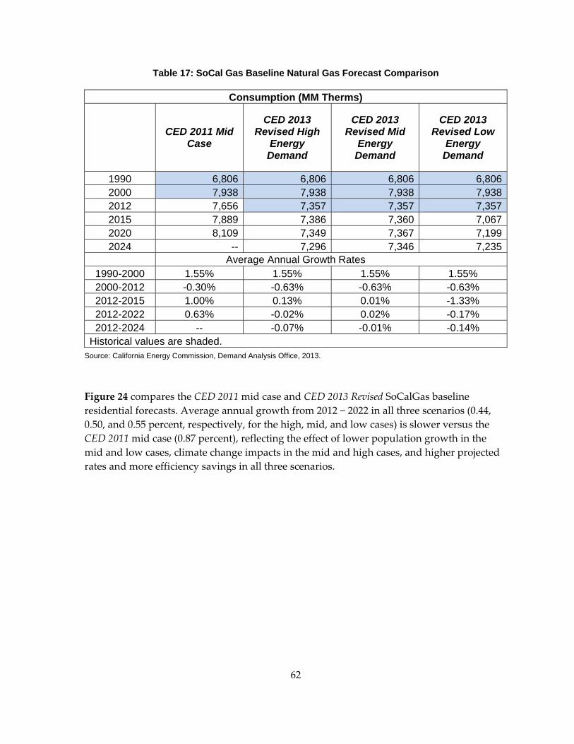
62

Table 17: SoCal Gas Baseline Natural Gas Forecast Comparison


CED 2011 Mid Case


Energy Demand


Energy Demand


Energy Demand

1990 6,806 6,806 6,806 6,8062000 7,938 7,938 7,938 7,9382012 7,656 7,357 7,357 7,3572015 7,889 7,386 7,360 7,0672020 8,109 7,349 7,367 7,1992024 -- 7,296 7,346 7,235

Average Annual Growth Rates 1990-2000 1.55% 1.55% 1.55% 1.55% 2000-2012 -0.30% -0.63% -0.63% -0.63% 2012-2015 1.00% 0.13% 0.01% -1.33% 2012-2022 0.63% -0.02% 0.02% -0.17% 2012-2024 -- -0.07% -0.01% -0.14%


Figure 24 compares the CED 2011 mid case and CED 2013 Revised SoCalGas baseline residential forecasts. Average annual growth from 2012 − 2022 in all three scenarios (0.44, 0.50, and 0.55 percent, respectively, for the high, mid, and low cases) is slower versus the CED 2011 mid case (0.87 percent), reflecting the effect of lower population growth in the mid and low cases, climate change impacts in the mid and high cases, and higher projected rates and more efficiency savings in all three scenarios.

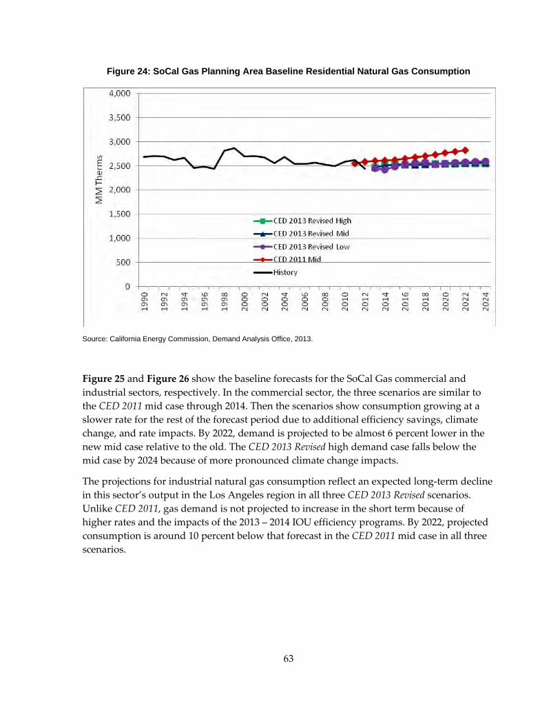
63

Figure 24: SoCal Gas Planning Area Baseline Residential Natural Gas Consumption


Figure 25 and Figure 26 show the baseline forecasts for the SoCal Gas commercial and industrial sectors, respectively. In the commercial sector, the three scenarios are similar to the CED 2011 mid case through 2014. Then the scenarios show consumption growing at a slower rate for the rest of the forecast period due to additional efficiency savings, climate change, and rate impacts. By 2022, demand is projected to be almost 6 percent lower in the new mid case relative to the old. The CED 2013 Revised high demand case falls below the mid case by 2024 because of more pronounced climate change impacts.

The projections for industrial natural gas consumption reflect an expected long‐term decline in this sector’s output in the Los Angeles region in all three CED 2013 Revised scenarios. Unlike CED 2011, gas demand is not projected to increase in the short term because of higher rates and the impacts of the 2013 – 2014 IOU efficiency programs. By 2022, projected consumption is around 10 percent below that forecast in the CED 2011 mid case in all three scenarios.

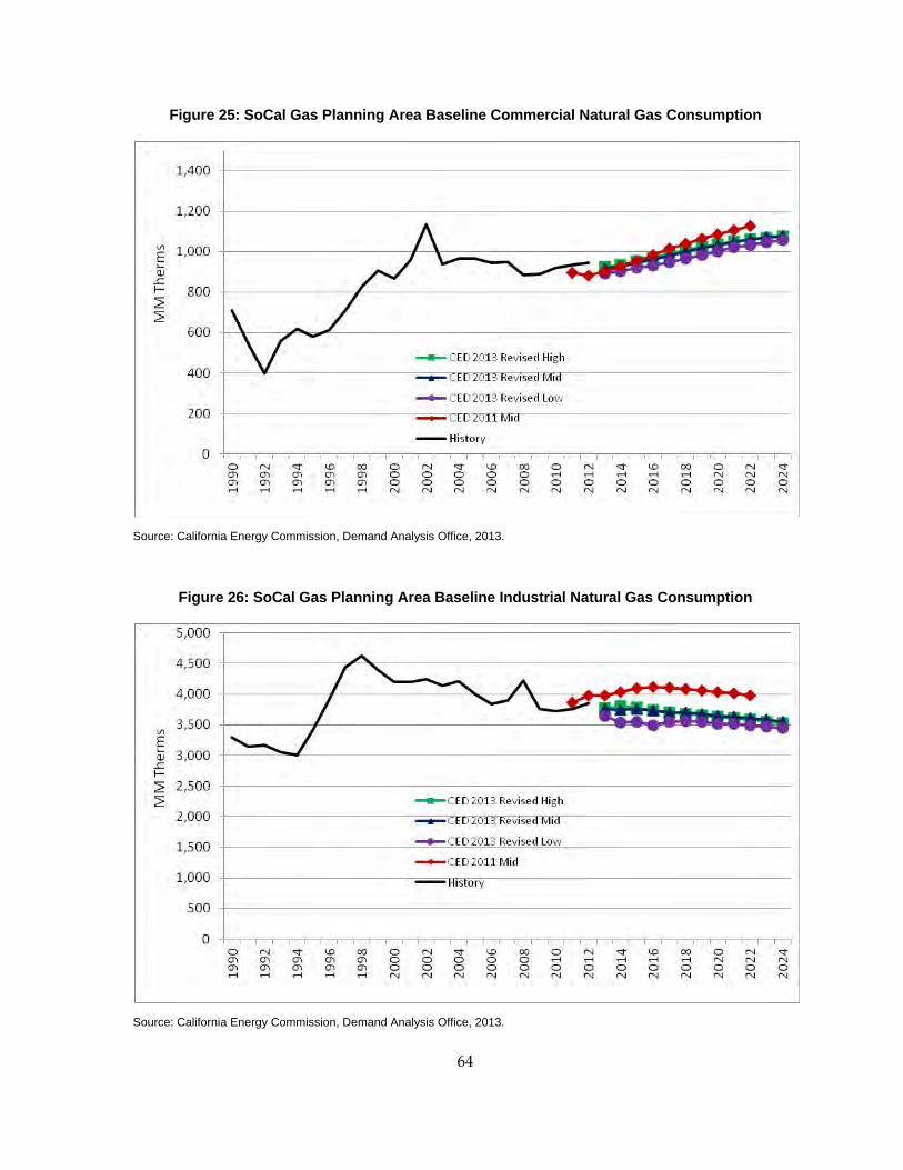
64

Figure 25: SoCal Gas Planning Area Baseline Commercial Natural Gas Consumption


Figure 26: SoCal Gas Planning Area Baseline Industrial Natural Gas Consumption


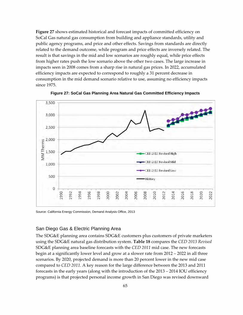
65

Figure 27 shows estimated historical and forecast impacts of committed efficiency on SoCal Gas natural gas consumption from building and appliance standards, utility and public agency programs, and price and other effects. Savings from standards are directly related to the demand outcome, while program and price effects are inversely related. The result is that savings in the mid and low scenarios are roughly equal, while price effects from higher rates push the low scenario above the other two cases. The large increase in impacts seen in 2008 comes from a sharp rise in natural gas prices. In 2022, accumulated efficiency impacts are expected to correspond to roughly a 31 percent decrease in consumption in the mid demand scenario relative to use, assuming no efficiency impacts since 1975.

Figure 27: SoCal Gas Planning Area Natural Gas Committed Efficiency Impacts


San Diego Gas & Electric Planning Area The SDG&E planning area contains SDG&E customers plus customers of private marketers using the SDG&E natural gas distribution system. Table 18 compares the CED 2013 Revised SDG&E planning area baseline forecasts with the CED 2011 mid case. The new forecasts begin at a significantly lower level and grow at a slower rate from 2012 – 2022 in all three scenarios. By 2020, projected demand is more than 20 percent lower in the new mid case compared to CED 2011. A key reason for the large difference between the 2013 and 2011 forecasts in the early years (along with the introduction of the 2013 – 2014 IOU efficiency programs) is that projected personal income growth in San Diego was revised downward

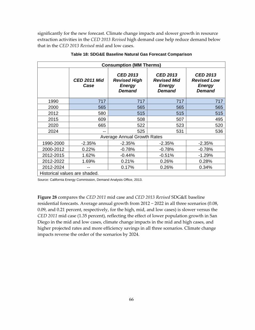
66

significantly for the new forecast. Climate change impacts and slower growth in resource extraction activities in the CED 2013 Revised high demand case help reduce demand below that in the CED 2013 Revised mid and low cases.

Table 18: SDG&E Baseline Natural Gas Forecast Comparison


CED 2011 Mid Case


Energy Demand


Energy Demand


Energy Demand

1990 717 717 717 7172000 565 565 565 5652012 580 515 515 5152015 609 508 507 4952020 665 522 523 5202024 -- 525 531 536

Average Annual Growth Rates 1990-2000 -2.35% -2.35% -2.35% -2.35% 2000-2012 0.22% -0.78% -0.78% -0.78% 2012-2015 1.62% -0.44% -0.51% -1.29% 2012-2022 1.69% 0.21% 0.26% 0.28% 2012-2024 -- 0.17% 0.26% 0.34%


Figure 28 compares the CED 2011 mid case and CED 2013 Revised SDG&E baseline residential forecasts. Average annual growth from 2012 − 2022 in all three scenarios (0.08, 0.09, and 0.21 percent, respectively, for the high, mid, and low cases) is slower versus the CED 2011 mid case (1.35 percent), reflecting the effect of lower population growth in San Diego in the mid and low cases, climate change impacts in the mid and high cases, and higher projected rates and more efficiency savings in all three scenarios. Climate change impacts reverse the order of the scenarios by 2024.

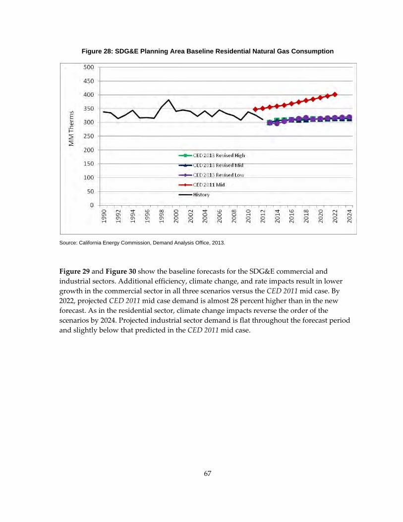
67

Figure 28: SDG&E Planning Area Baseline Residential Natural Gas Consumption


Figure 29 and Figure 30 show the baseline forecasts for the SDG&E commercial and industrial sectors. Additional efficiency, climate change, and rate impacts result in lower growth in the commercial sector in all three scenarios versus the CED 2011 mid case. By 2022, projected CED 2011 mid case demand is almost 28 percent higher than in the new forecast. As in the residential sector, climate change impacts reverse the order of the scenarios by 2024. Projected industrial sector demand is flat throughout the forecast period and slightly below that predicted in the CED 2011 mid case.

68

Figure 29: SDG&E Planning Area Baseline Commercial Natural Gas Consumption


Figure 30: SDG&E Planning Area Baseline Industrial Natural Gas Consumption


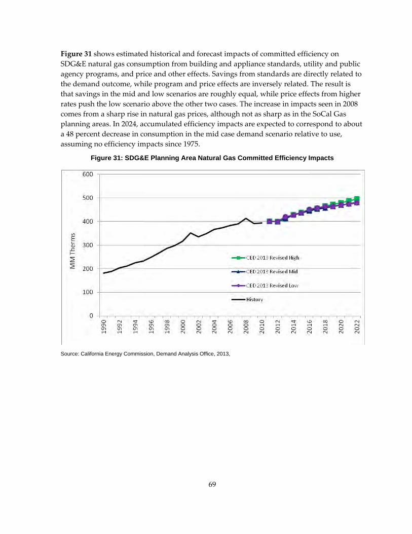
69

Figure 31 shows estimated historical and forecast impacts of committed efficiency on SDG&E natural gas consumption from building and appliance standards, utility and public agency programs, and price and other effects. Savings from standards are directly related to the demand outcome, while program and price effects are inversely related. The result is that savings in the mid and low scenarios are roughly equal, while price effects from higher rates push the low scenario above the other two cases. The increase in impacts seen in 2008 comes from a sharp rise in natural gas prices, although not as sharp as in the SoCal Gas planning areas. In 2024, accumulated efficiency impacts are expected to correspond to about a 48 percent decrease in consumption in the mid case demand scenario relative to use, assuming no efficiency impacts since 1975.

Figure 31: SDG&E Planning Area Natural Gas Committed Efficiency Impacts

Source: California Energy Commission, Demand Analysis Office, 2013,

70

CHAPTER 3: Energy Efficiency and Conservation

Introduction

With the state’s adoption of the first Energy Action Plan in 2003, energy efficiency became the resource of first choice for meeting the state’s future energy needs. Under Assembly Bill 2021 (Levine, Chapter 734, Statutes of 2006) (AB 2021), the Energy Commission, in consultation with the CPUC, is responsible for periodically developing annual statewide efficiency potential estimates and setting savings targets in a public process using the most recent IOU and POU data. These targets, combined with California’s greenhouse gas emission reduction goals, make it essential for the Energy Commission to account for energy efficiency impacts when forecasting future electricity and natural gas demand.

Starting with the 2009 IEPR process, staff has undertaken a major effort to improve and refine efficiency measurement within the IEPR forecast and committed to examining methods for incorporating efficiency impacts in a public process that includes the CPUC staff, utilities, and other stakeholders. With this commitment in mind, Energy Commission staff continues its involvement in and support for the Demand Analysis Working Group, which provides a forum for interaction among key organizations on topics related to demand forecasting and demand‐side programs and policies. Membership in the Demand Analysis Working Group includes staff from the Energy Commission, the CPUC Energy Division, the Department of Ratepayer Advocates, the California IOUs, several POUs, and other interested parties, including the California Air Resources Board, The Utility Reform Network, and the NRDC. The member list has grown to include more than 100 participants.

With input from the Demand Analysis Working Group, a substantial amount of work was dedicated to improving estimates of efficiency impacts incorporated in CED 2009 and CED 2011. CED 2013 Revised builds on this work and incorporates the following elements:

• New building and appliance standards, including impacts from the 2013 Title 24 building standards update and the 2011 battery charger standards

• IOU 2013‐2014 efficiency programs

• Updated program savings for POUs, using estimated first‐year savings through 2013

• Updated price elasticity estimates

Committed Energy Efficiency

The baseline forecast incorporates savings in energy demand associated with three sources: committed utility and public agency efficiency programs; finalized or implemented

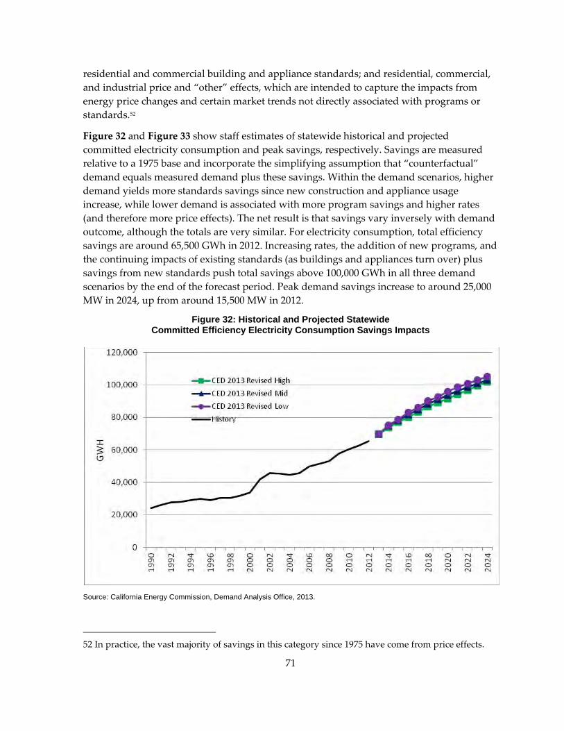
71

residential and commercial building and appliance standards; and residential, commercial, and industrial price and “other” effects, which are intended to capture the impacts from energy price changes and certain market trends not directly associated with programs or standards.52

Figure 32 and Figure 33 show staff estimates of statewide historical and projected committed electricity consumption and peak savings, respectively. Savings are measured relative to a 1975 base and incorporate the simplifying assumption that “counterfactual” demand equals measured demand plus these savings. Within the demand scenarios, higher demand yields more standards savings since new construction and appliance usage increase, while lower demand is associated with more program savings and higher rates (and therefore more price effects). The net result is that savings vary inversely with demand outcome, although the totals are very similar. For electricity consumption, total efficiency savings are around 65,500 GWh in 2012. Increasing rates, the addition of new programs, and the continuing impacts of existing standards (as buildings and appliances turn over) plus savings from new standards push total savings above 100,000 GWh in all three demand scenarios by the end of the forecast period. Peak demand savings increase to around 25,000 MW in 2024, up from around 15,500 MW in 2012.

Figure 32: Historical and Projected Statewide Committed Efficiency Electricity Consumption Savings Impacts


52 In practice, the vast majority of savings in this category since 1975 have come from price effects.

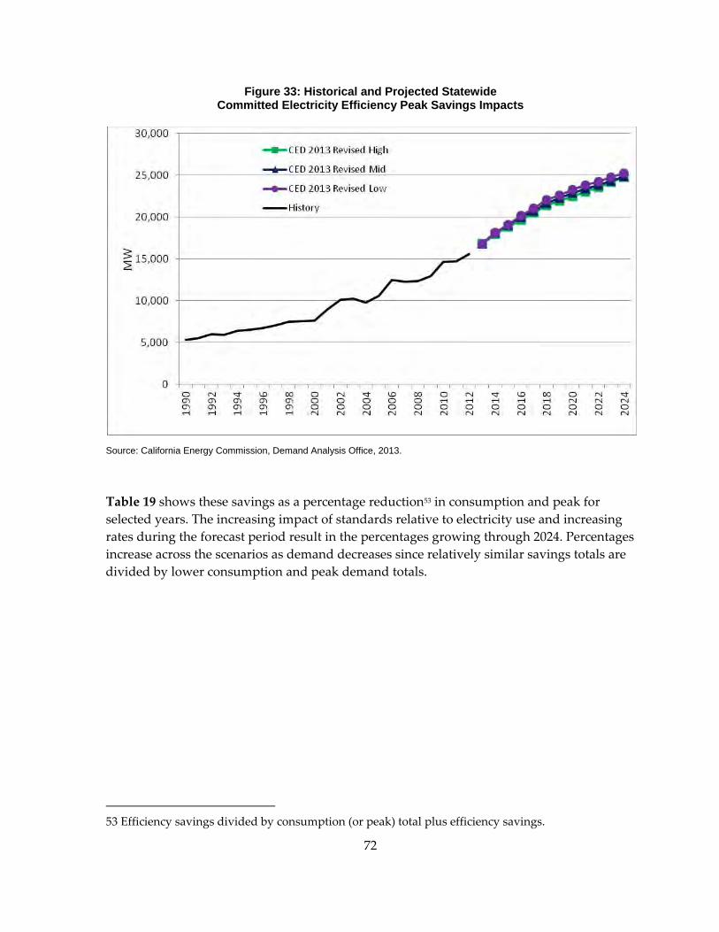
72

Figure 33: Historical and Projected Statewide Committed Electricity Efficiency Peak Savings Impacts


Table 19 shows these savings as a percentage reduction53 in consumption and peak for selected years. The increasing impact of standards relative to electricity use and increasing rates during the forecast period result in the percentages growing through 2024. Percentages increase across the scenarios as demand decreases since relatively similar savings totals are divided by lower consumption and peak demand totals.

53 Efficiency savings divided by consumption (or peak) total plus efficiency savings.

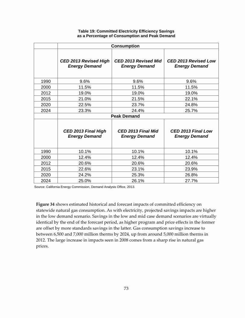
73

Table 19: Committed Electricity Efficiency Savings as a Percentage of Consumption and Peak Demand

Consumption

CED 2013 Revised High Energy Demand

CED 2013 Revised Mid Energy Demand

CED 2013 Revised Low Energy Demand

1990 9.6% 9.6% 9.6% 2000 11.5% 11.5% 11.5% 2012 19.0% 19.0% 19.0% 2015 21.0% 21.5% 22.1% 2020 22.5% 23.7% 24.8% 2024 23.3% 24.4% 25.7%

Peak Demand

CED 2013 Final High Energy Demand

CED 2013 Final Mid Energy Demand

CED 2013 Final Low Energy Demand

1990 10.1% 10.1% 10.1% 2000 12.4% 12.4% 12.4% 2012 20.6% 20.6% 20.6% 2015 22.6% 23.1% 23.9% 2020 24.2% 25.3% 26.8% 2024 25.0% 26.1% 27.7%


Figure 34 shows estimated historical and forecast impacts of committed efficiency on statewide natural gas consumption. As with electricity, projected savings impacts are higher in the low demand scenario. Savings in the low and mid case demand scenarios are virtually identical by the end of the forecast period, as higher program and price effects in the former are offset by more standards savings in the latter. Gas consumption savings increase to between 6,500 and 7,000 million therms by 2024, up from around 5,000 million therms in 2012. The large increase in impacts seen in 2008 comes from a sharp rise in natural gas prices.

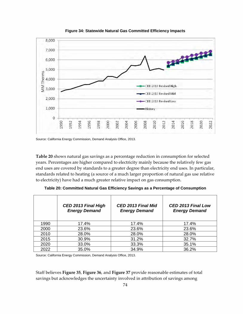
74

Figure 34: Statewide Natural Gas Committed Efficiency Impacts


Table 20 shows natural gas savings as a percentage reduction in consumption for selected years. Percentages are higher compared to electricity mainly because the relatively few gas end uses are covered by standards to a greater degree than electricity end uses. In particular, standards related to heating (a source of a much larger proportion of natural gas use relative to electricity) have had a much greater relative impact on gas consumption.

Table 20: Committed Natural Gas Efficiency Savings as a Percentage of Consumption

CED 2013 Final High Energy Demand

CED 2013 Final Mid Energy Demand

CED 2013 Final Low Energy Demand

1990 17.4% 17.4% 17.4%2000 23.6% 23.6% 23.6%2010 28.0% 28.0% 28.0%2015 30.9% 31.2% 32.7%2020 33.0% 33.3% 35.1%2022 35.0% 34.9% 36.2%


Staff believes Figure 35, Figure 36, and Figure 37 provide reasonable estimates of total savings but acknowledges the uncertainty involved in attribution of savings among

75

standards, programs, and price effects, especially during the historical period. Standards and programs are often designed to work together to reduce a targeted usage, and rate hikes increase the likelihood of participating in an incentive program or complying with a given standard. Therefore, no attribution among the three sources is shown, except for estimates of standards impacts and future committed program savings presented later in this chapter.

Committed Efficiency Programs Historical electricity and natural gas program impacts were treated similarly to CED 2011,54 with both POU and IOU savings through 2012 incorporating the most recent CPUC evaluation, measurement, and verification studies.55 First‐year utility‐reported net savings are adjusted at the end‐use level using realization rates56 derived from these studies. These savings are then decayed (adjusted in each year by estimated rate of product failure) over the forecast period using expected useful measure lives from the most recent Database for Energy Efficient Resources (DEER) and applying an exponential decay function.

For the 2013 – 2014 IOU programs, staff relied on utility‐projected net savings, translating measure‐level detail to the appropriate end uses required for the forecast. Utilities were required to estimate measure impacts to be consistent with CPUC evaluation, measurement, and verification studies, so staff felt comfortable applying these savings without additional adjustments (such as realization rates), unlike past program cycles. Decay by end use was then reduced by 50 percent to reflect the CPUC’s directive that one‐half of measure decay be replaced through additional program activities.57

Figure 35 and Figure 36 show resulting projected 2013 – 2014 IOU cumulative program consumption savings for electricity and natural gas, respectively, over the forecast period. These savings were used in the mid demand case. Electricity savings for the combined IOUs reach almost 2,500 GWh in 2014 and decay to around 1,800 GWh by 2024. Combined savings for natural gas are estimated at around 80 million therms in 2014, decreasing to about 68 million therms in 2024. As alternative program scenarios for the other demand

54 California Energy Commission. June 2012. California Energy Demand 2012 – 2022 Final Forecast. CEC‐200‐2012‐001‐CMF‐V1. Chapter 3: Efficiency and Conservation http://www.energy.ca.gov/2012publications/CEC‐200‐2012‐001/CEC‐200‐2012‐001‐CMF‐V1.pdf.

55 The CPUC is working on a review of 2010– 2012 program accomplishments, so final results are not yet available for this forecast.

56 Realization rates are meant to be an adjustment for real‐world phenomena that may reduce measure savings. For example, compact fluorescents that are purchased but never installed.

57 CPUC Decision 09‐09‐047, September 2009. This requirement applies to all IOU programs starting with 2006 first‐year savings.

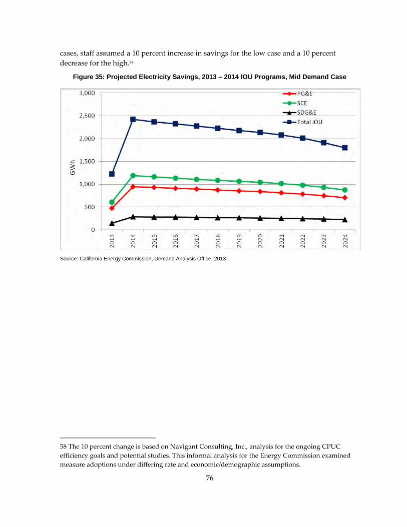
76

cases, staff assumed a 10 percent increase in savings for the low case and a 10 percent decrease for the high.58

Figure 35: Projected Electricity Savings, 2013 – 2014 IOU Programs, Mid Demand Case


58 The 10 percent change is based on Navigant Consulting, Inc., analysis for the ongoing CPUC efficiency goals and potential studies. This informal analysis for the Energy Commission examined measure adoptions under differing rate and economic/demographic assumptions.

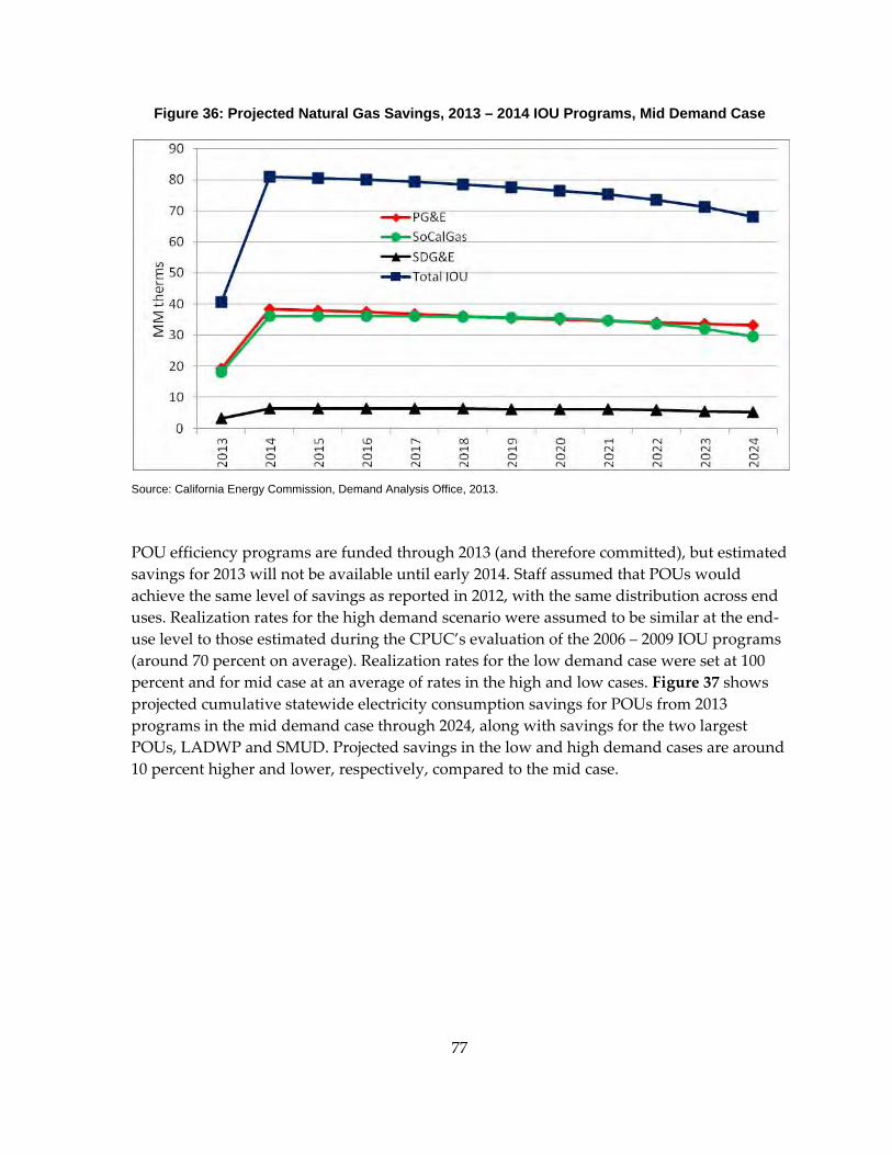
77

Figure 36: Projected Natural Gas Savings, 2013 – 2014 IOU Programs, Mid Demand Case


POU efficiency programs are funded through 2013 (and therefore committed), but estimated savings for 2013 will not be available until early 2014. Staff assumed that POUs would achieve the same level of savings as reported in 2012, with the same distribution across end uses. Realization rates for the high demand scenario were assumed to be similar at the end‐use level to those estimated during the CPUC’s evaluation of the 2006 – 2009 IOU programs (around 70 percent on average). Realization rates for the low demand case were set at 100 percent and for mid case at an average of rates in the high and low cases. Figure 37 shows projected cumulative statewide electricity consumption savings for POUs from 2013 programs in the mid demand case through 2024, along with savings for the two largest POUs, LADWP and SMUD. Projected savings in the low and high demand cases are around 10 percent higher and lower, respectively, compared to the mid case.

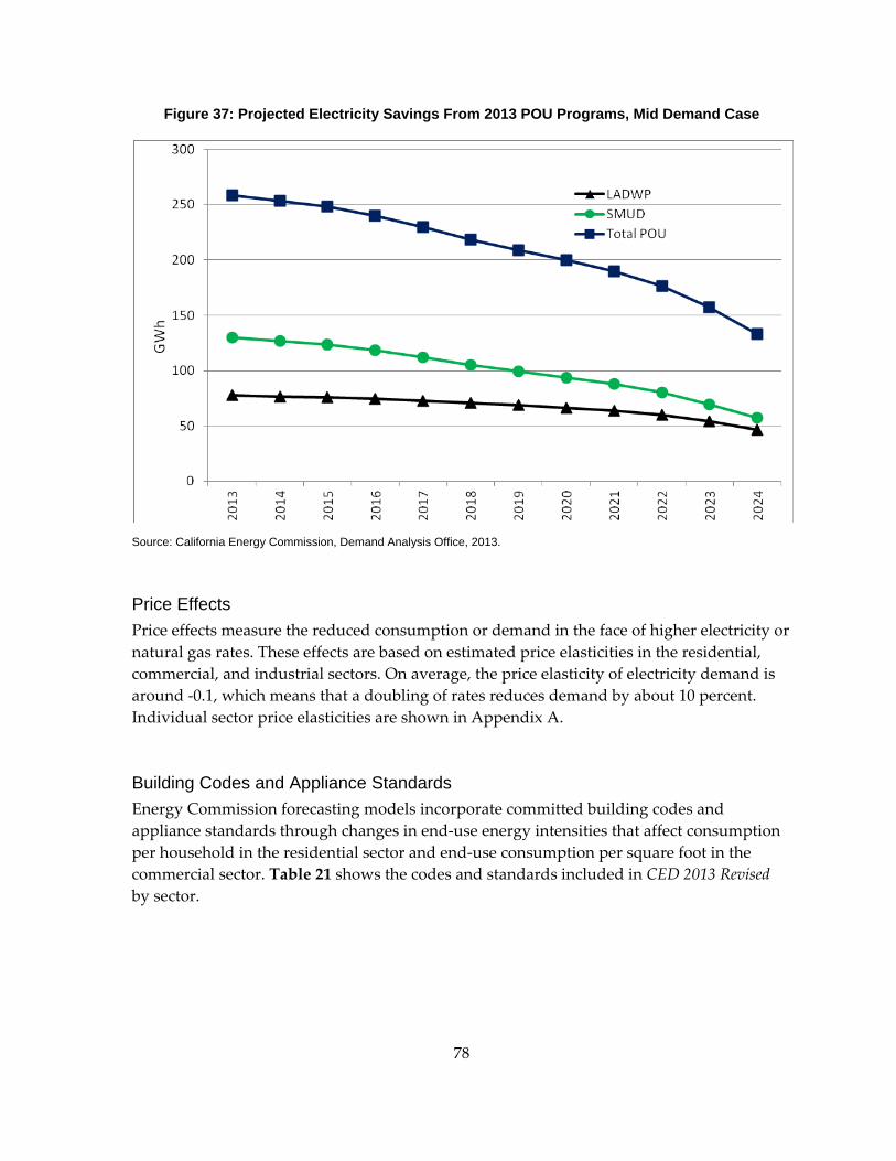
78

Figure 37: Projected Electricity Savings From 2013 POU Programs, Mid Demand Case


Price Effects Price effects measure the reduced consumption or demand in the face of higher electricity or natural gas rates. These effects are based on estimated price elasticities in the residential, commercial, and industrial sectors. On average, the price elasticity of electricity demand is around ‐0.1, which means that a doubling of rates reduces demand by about 10 percent. Individual sector price elasticities are shown in Appendix A.

Building Codes and Appliance Standards Energy Commission forecasting models incorporate committed building codes and appliance standards through changes in end‐use energy intensities that affect consumption per household in the residential sector and end‐use consumption per square foot in the commercial sector. Table 21 shows the codes and standards included in CED 2013 Revised by sector.

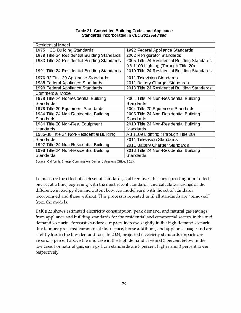
79

Table 21: Committed Building Codes and Appliance Standards Incorporated in CED 2013 Revised

Residential Model 1975 HCD Building Standards 1992 Federal Appliance Standards 1978 Title 24 Residential Building Standards 2002 Refrigerator Standards 1983 Title 24 Residential Building Standards 2005 Title 24 Residential Building Standards

1991 Title 24 Residential Building Standards AB 1109 Lighting (Through Title 20) 2010 Title 24 Residential Building Standards

1976-82 Title 20 Appliance Standards 1988 Federal Appliance Standards

2011 Television Standards 2011 Battery Charger Standards

1990 Federal Appliance Standards 2013 Title 24 Residential Building Standards Commercial Model 1978 Title 24 Nonresidential Building Standards

2001 Title 24 Non-Residential Building Standards

1978 Title 20 Equipment Standards 2004 Title 20 Equipment Standards 1984 Title 24 Non-Residential Building Standards


1984 Title 20 Non-Res. Equipment Standards


1985-88 Title 24 Non-Residential Building AB 1109 Lighting (Through Title 20) Standards 2011 Television Standards 1992 Title 24 Non-Residential Building 2011 Battery Charger Standards 1998 Title 24 Non-Residential Building Standards



To measure the effect of each set of standards, staff removes the corresponding input effect one set at a time, beginning with the most recent standards, and calculates savings as the difference in energy demand output between model runs with the set of standards incorporated and those without. This process is repeated until all standards are “removed” from the models.

Table 22 shows estimated electricity consumption, peak demand, and natural gas savings from appliance and building standards for the residential and commercial sectors in the mid demand scenario. Forecast standards impacts increase slightly in the high demand scenario due to more projected commercial floor space, home additions, and appliance usage and are slightly less in the low demand case. In 2024, projected electricity standards impacts are around 5 percent above the mid case in the high demand case and 3 percent below in the low case. For natural gas, savings from standards are 7 percent higher and 3 percent lower, respectively.

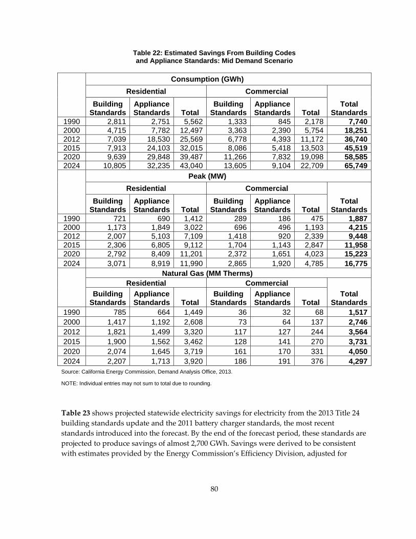
80

Table 22: Estimated Savings From Building Codes and Appliance Standards: Mid Demand Scenario

Consumption (GWh) Residential Commercial Building

Standards Appliance Standards Total

Building Standards

Appliance Standards Total

Total Standards

1990 2,811 2,751 5,562 1,333 845 2,178 7,7402000 4,715 7,782 12,497 3,363 2,390 5,754 18,2512012 7,039 18,530 25,569 6,778 4,393 11,172 36,7402015 7,913 24,103 32,015 8,086 5,418 13,503 45,5192020 9,639 29,848 39,487 11,266 7,832 19,098 58,5852024 10,805 32,235 43,040 13,605 9,104 22,709 65,749

Peak (MW) Residential Commercial

Building Standards


Building Standards


Total Standards

1990 721 690 1,412 289 186 475 1,8872000 1,173 1,849 3,022 696 496 1,193 4,2152012 2,007 5,103 7,109 1,418 920 2,339 9,4482015 2,306 6,805 9,112 1,704 1,143 2,847 11,9582020 2,792 8,409 11,201 2,372 1,651 4,023 15,2232024 3,071 8,919 11,990 2,865 1,920 4,785 16,775

Natural Gas (MM Therms) Residential Commercial

Total Standards

Building Standards


Building Standards


1990 785 664 1,449 36 32 68 1,5172000 1,417 1,192 2,608 73 64 137 2,7462012 1,821 1,499 3,320 117 127 244 3,5642015 1,900 1,562 3,462 128 141 270 3,7312020 2,074 1,645 3,719 161 170 331 4,0502024 2,207 1,713 3,920 186 191 376 4,297



Table 23 shows projected statewide electricity savings for electricity from the 2013 Title 24 building standards update and the 2011 battery charger standards, the most recent standards introduced into the forecast. By the end of the forecast period, these standards are projected to produce savings of almost 2,700 GWh. Savings were derived to be consistent with estimates provided by the Energy Commission’s Efficiency Division, adjusted for

81

noncompliance (assumed to be 15 percent59) and “naturally occurring” adoptions of relevant technologies.60 The Title 24 update also provides an estimated 22 million therms of natural gas savings by 2024.

Table 23: Estimated Statewide Electricity Savings* (GWh) From 2013 Title 24 Building Standards Update and 2011 Battery Charger Standards

Year Title 24 Update Battery Charger Standards

Total

2015 162 460 622

2018 613 850 1,463

2020 932 1,083 2,015

2024 1,546 1,147 2,693


*Projected unadjusted (gross) savings reach more than 2,900 GWh for Title 24 and more than 1,900 GWh for battery chargers by 2024.


Incremental Achievable Efficiency Savings

Committed efficiency savings reflect savings from initiatives that have been approved, finalized, and funded, whether already implemented or not. There are potential additional savings from initiatives that have not been finalized or funded but are reasonably likely to occur, and include impacts from future updates of building and appliance standards and utility efficiency programs expected to be implemented after 2014. These savings are referred to as achievable. Staff is completing an analysis of achievable savings incremental to the baseline forecast, based on the 2013 California Energy Efficiency Potential and Goals Study, completed for the CPUC by Navigant Consulting, Inc., in August 2013.61 Results from this analysis will be presented along with the baseline forecast during the IEPR demand forecast 59 Based on CPUC. Final Evaluation Report, Codes & Standards (C&S) Programs Impact Evaluation, California Investor Owned Utilities’ Codes and Standards Program Evaluation for Program Years 2006–2008. Prepared by KEMA, Inc., The Cadmus Group, Inc., Itron, Inc., and Nexus Market Research, Inc.

60 As estimated by Navigant Consulting, Inc., for the CPUC’s 2012 efficiency potential study: Analysis to Update Energy Efficiency Potential, Goals, and Targets for 2013 and Beyond: Track 1 Statewide Investor‐Owned Utility Energy Efficiency Potential Study, available at http://www.cpuc.ca.gov/NR/rdonlyres/6FF9C18B‐CAA0‐4D63‐ACC6‐F9CB4EB1590B/0/2011IOUServiceTerritoryEEPotentialStudy.pdf.

61 See http://demandanalysisworkinggroup.org/documents/2013_08_16_ES_Pup_EE_Pot_final/CA_PGT_ Model_2012_2013_Release_Aug_2013.ana.zip.

82

workshop on October 1, 2013. These results will be used to develop an adjusted forecast for resource planning. A staff paper documenting the analysis and results will be released before the workshop.

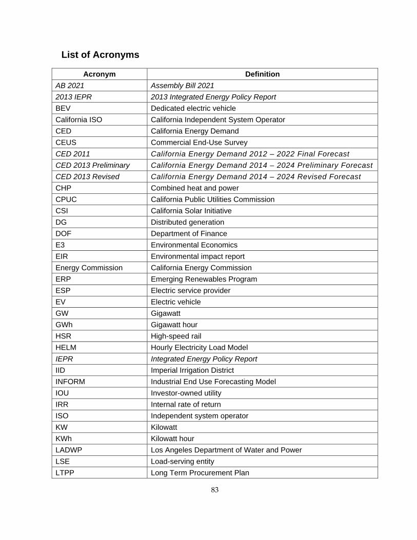
83

List of Acronyms

Acronym Definition AB 2021 Assembly Bill 2021 2013 IEPR 2013 Integrated Energy Policy Report BEV Dedicated electric vehicle California ISO California Independent System Operator CED California Energy Demand CEUS Commercial End-Use Survey CED 2011 California Energy Demand 2012 – 2022 Final Forecast CED 2013 Preliminary California Energy Demand 2014 – 2024 Preliminary Forecast CED 2013 Revised California Energy Demand 2014 – 2024 Revised Forecast CHP Combined heat and power CPUC California Public Utilities Commission CSI California Solar Initiative DG Distributed generation DOF Department of Finance E3 Environmental Economics EIR Environmental impact report Energy Commission California Energy Commission ERP Emerging Renewables Program ESP Electric service provider EV Electric vehicle GW Gigawatt GWh Gigawatt hour HSR High-speed rail HELM Hourly Electricity Load Model IEPR Integrated Energy Policy Report IID Imperial Irrigation District INFORM Industrial End Use Forecasting Model IOU Investor-owned utility IRR Internal rate of return ISO Independent system operator KW Kilowatt KWh Kilowatt hour LADWP Los Angeles Department of Water and Power LSE Load-serving entity LTPP Long Term Procurement Plan

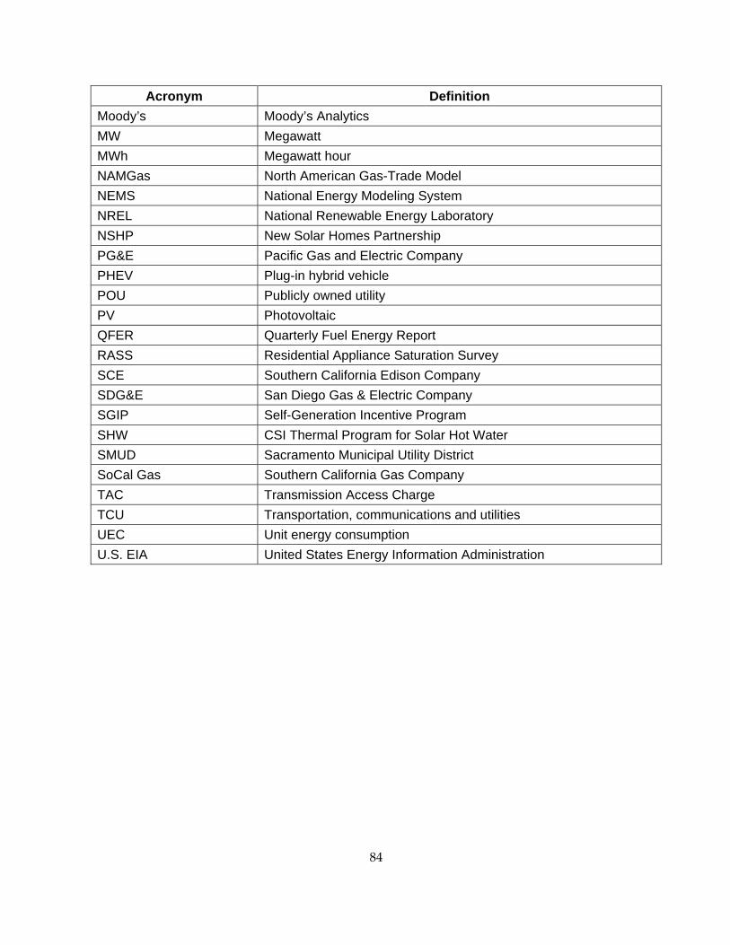
84

Acronym Definition Moody’s Moody’s Analytics MW Megawatt MWh Megawatt hour NAMGas North American Gas-Trade Model NEMS National Energy Modeling System NREL National Renewable Energy Laboratory NSHP New Solar Homes Partnership PG&E Pacific Gas and Electric Company PHEV Plug-in hybrid vehicle POU Publicly owned utility PV Photovoltaic QFER Quarterly Fuel Energy Report RASS Residential Appliance Saturation Survey SCE Southern California Edison Company SDG&E San Diego Gas & Electric Company SGIP Self-Generation Incentive Program SHW CSI Thermal Program for Solar Hot Water SMUD Sacramento Municipal Utility District SoCal Gas Southern California Gas Company TAC Transmission Access Charge TCU Transportation, communications and utilities UEC Unit energy consumption U.S. EIA United States Energy Information Administration

A‐1

APPENDIX A: Additional Methodology Documentation and Econometric Results This appendix provides additional detail on forecasting methodology, including the new industrial model, incorporation of potential climate change impacts, and price elasticities of demand assumed for the forecast. In addition, the appendix compares CED 2013 Revised results with the econometric forecasts.

Industrial Model

Until this forecast, staff has used the INFORM, developed by the Electric Power Research Institute, to forecast industrial sector energy use. However, the model is no longer supported by Electric Power Research Institute, and the original contract agreement did not include the program code for the model, making improvements and revisions very difficult. Therefore, staff decided to develop a new model from the “ground up,” based on the INFORM method, so that improvements, revisions, and augmentations could be made as needed.

As in the INFORM model, industrial (manufacturing, resource extraction, and construction) energy demand is forecast based on projected growth in dollar output or employment for 28 categories (for example, chemicals and paper), projected average industrial rates, and changes in end‐use characteristics, including energy intensities.62 In this context, energy intensity measures energy use per dollar of output. The marginal impact of economic growth on energy use in each of the 28 categories was estimated using regression analysis. Applying the estimated coefficients to the appropriate economic indicator provides a “business as usual” forecast for each industrial category. This forecast is adjusted for rate increases, using price elasticities estimated in the sector econometric models.63 Finally, the forecast is adjusted to account for changes in end‐use energy intensity.

Unfortunately, recent data on industrial end‐use energy intensities and other characteristics to fully populate the model are not available for California. A full statewide industrial survey has not been administered for more than 20 years. For CED 2013 Revised, staff made simplifying assumptions for future end‐use energy intensity trends using econometric analysis of historical data. For manufacturing as a whole, this analysis showed a roughly 1 percent annual energy intensity decrease on average (for all end uses combined) over the 1980 – 2012 period. For the CED 2013 Revised low demand scenario, this trend was assumed 62 End uses include motors; thermal processes; other processes; lighting; heating, ventilation, and air conditioning; and miscellaneous.

63 See Table A‐6.

A‐2

to continue for every subsector and end use through 2024. For the mid and high cases, the trend was reduced to 0.5 percent and 0.25 percent per year, respectively. Construction and resource extraction historical data showed no clear trend, and intensities were assumed constant over the forecast period.

Staff is beginning to populate end‐use characteristics in the model using national data and smaller‐scale state surveys. Ultimately, however, the new model will require a full California industrial end‐use survey to reach full potential as a forecasting tool.

Comparison of CED 2013 Revised and Full Econometric Forecasts

Table A‐1 compares CED 2013 Revised electricity results for 2024 by major planning area and statewide with those from a full econometric forecast. More complete results are provided along with the demand forms posted with this report.64 For consumption, differences range from around zero to almost 4.5 percent above for the econometric forecasts. Peak demand differs from around 0.5 percent higher to around 5 percent higher. Likely reasons for these differences are discussed in Chapter 1 of this volume. Differences are largest for LADWP peak demand and smallest for SMUD consumption.

Table A‐2 compares CED 2013 Revised end‐user natural gas results for 2024 by major planning area and statewide with those from a full econometric forecast. Differences range from around 5 percent higher for the econometric forecast to almost 12 percent higher. Most of the differences come from the residential sector, reflecting increases in efficiency impacts not fully reflected in the econometric results.

64 See http://www.energy.ca.gov/2013_energypolicy/documents/2013‐05‐30_workshop/spreadsheets/.

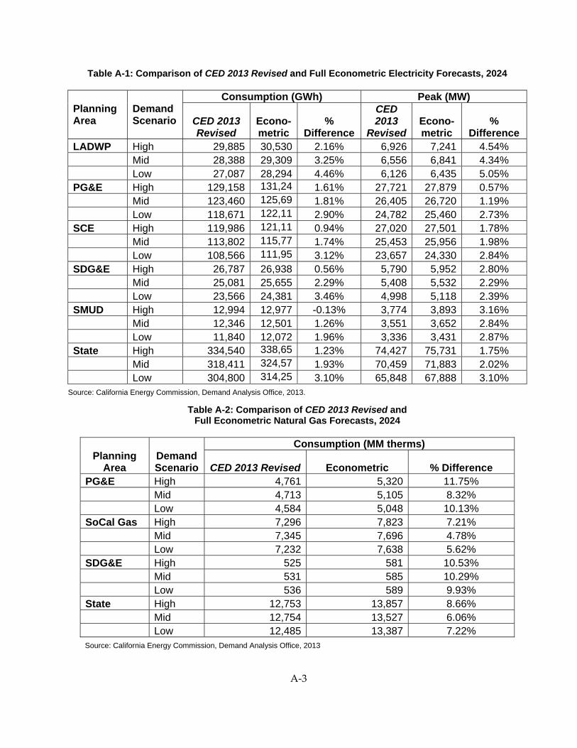
A‐3

Table A-1: Comparison of CED 2013 Revised and Full Econometric Electricity Forecasts, 2024

Planning Area

Demand Scenario

Consumption (GWh) Peak (MW)

CED 2013 Revised

Econo-metric

% Difference

CED 2013

Revised Econo-metric

% Difference

LADWP High 29,885 30,530 2.16% 6,926 7,241 4.54% Mid 28,388 29,309 3.25% 6,556 6,841 4.34% Low 27,087 28,294 4.46% 6,126 6,435 5.05% PG&E High 129,158 131,24 1.61% 27,721 27,879 0.57% Mid 123,460 125,69 1.81% 26,405 26,720 1.19% Low 118,671 122,11 2.90% 24,782 25,460 2.73% SCE High 119,986 121,11 0.94% 27,020 27,501 1.78% Mid 113,802 115,77 1.74% 25,453 25,956 1.98% Low 108,566 111,95 3.12% 23,657 24,330 2.84% SDG&E High 26,787 26,938 0.56% 5,790 5,952 2.80% Mid 25,081 25,655 2.29% 5,408 5,532 2.29% Low 23,566 24,381 3.46% 4,998 5,118 2.39% SMUD High 12,994 12,977 -0.13% 3,774 3,893 3.16% Mid 12,346 12,501 1.26% 3,551 3,652 2.84% Low 11,840 12,072 1.96% 3,336 3,431 2.87% State High 334,540 338,65 1.23% 74,427 75,731 1.75% Mid 318,411 324,57 1.93% 70,459 71,883 2.02% Low 304,800 314,25 3.10% 65,848 67,888 3.10%


Table A-2: Comparison of CED 2013 Revised and Full Econometric Natural Gas Forecasts, 2024

Planning

Area

Demand Scenario

Consumption (MM therms)

CED 2013 Revised Econometric % Difference PG&E High 4,761 5,320 11.75% Mid 4,713 5,105 8.32% Low 4,584 5,048 10.13% SoCal Gas High 7,296 7,823 7.21% Mid 7,345 7,696 4.78% Low 7,232 7,638 5.62% SDG&E High 525 581 10.53% Mid 531 585 10.29% Low 536 589 9.93% State High 12,753 13,857 8.66% Mid 12,754 13,527 6.06% Low 12,485 13,387 7.22% Source: California Energy Commission, Demand Analysis Office, 2013

A‐4

Impacts From Climate Change

CED 2013 Revised estimates the impacts of potential climate change for both energy (electricity and natural gas) and electricity peak demand. Energy impacts are estimated through changes in the number of annual heating and cooling degree days,65 while peak demand impacts are simulated though increases in annual maximum daily average temperatures.

Econometric models for the residential, commercial, industrial, and agricultural sectors yielded significant coefficients for degree days, either for electricity, natural gas, or both. (See Appendix C.) Electricity consumption is affected by both heating and cooling degree days, while natural gas is affected by heating degree days only. For electricity, the impact of increases in the average annual number of cooling degree days as a result of climate change is tempered by decreasing average heating degree days, since both minimum and maximum temperatures increase. Because of heating degree day decreases, end‐user natural gas demand drops, all else equal, due to climate change.

The econometric peak model re‐estimated for CED 2013 Revised includes a coefficient for the annual maximum of average631, defined as follows:

Average631 = Daily Average Temperature66 × 0.6 + Previous Day’s Average Temperature × 0.3 + Two Days’ Previous Average Temperature × 0.1.

The adjustment from a simple daily average temperature to average631 is meant to provide a better indicator of sustained temperature warming.67

To gauge the potential impact of climate change on annual degree days and average631 temperatures through 2024, staff used a 2012 update of a climate change impact assessment by the California Climate Change Center, sponsored by the Energy Commission.68 The update uses 24 climate change simulations for California consisting of two scenarios for each of 12 models, providing simulation results for daily maximum and minimum temperatures, average daily humidity, and sea level rises through 2099.

65 Heating and cooling degree days measure the difference between daily average temperature and a reference temperature (for example, 65 degrees) summed over all days in a given year. An average temperature below the reference temperature adds to heating degree days and an average above the reference adds to cooling degree days.

66 Defined as maximum plus minimum daily temperature divided by 2.

67 Evidence shows that response to high temperatures increases if warming is sustained over a period of days, as customers do not always adjust immediately to changing weather.

68 California Energy Commission. March 2009. Climate Change Scenarios and Sea Level Rise Estimates for the California 2008 Climate Change Scenarios Assessment.CEC‐500‐2009‐014‐D.

A‐5

Climate change model simulations were performed for grids of 50 square miles within the state; staff used simulated daily maximum and minimum temperatures for grids corresponding to the 10 weather stations used for the 16 forecasting climate zones. Staff chose climate change scenarios that resulted in an average temperature impact over all scenarios for the mid demand case and a relatively high temperature impact for the high demand case.69 For the low demand scenario, staff assumed no climate change impacts. Staff converted simulated daily averages for each weather station to degree days and average631 indices for each planning area by weighting each climate zone either by estimated number of air conditioners (average631 and cooling degree days) or population (heating degree days). Changes in annual degree days and maximum average631 temperatures starting in 2013 were derived using long‐term trends (2010‐2040) from the two climate scenarios.70

Table A‐3 shows the projected impacts of climate change in the mid and high demand scenarios on electricity consumption for the five major planning areas and for the state as a whole. By 2024, statewide consumption impacts reach almost 1,200 GWh in the mid demand case and almost 1,700 GWh in the high demand case. Also shown are the simulated annual heating and cooling degree days (weighted by climate zone) for the two climate change scenarios used. Degree days in 2012 represent a historical 30‐year average for the planning area.

The consumption increases shown in Table A‐3 are net impacts, representing increasing electricity consumption from cooling minus reduced usage from less heating need. Heating impacts are typically 10 – 40 percent of cooling increases, depending on the planning area and year. For the state as a whole in 2024, projected electricity consumption increases by more than 1,400 GWh from more cooling need in the mid demand case, all else equal, and decreases by around 250 GWh from less heating. In the high demand case, the totals are about 2,300 GWh and 600 GWh, respectively. For the state as a whole, the largest portions of the consumption increase come from the commercial sector (50 percent and 60 percent in the mid and high cases, respectively), since the effect from warmer temperatures is not mitigated by decreasing heating degree days, as in the residential sector (see Appendix C).

69 Staff wishes to thank Mary Tyree at the Scripps Institute of Oceanography for providing the simulation data.

70 A long‐term trend was used rather than the actual temperatures in each scenario because year‐to‐year fluctuations simulated in the climate change models sometimes resulted in degree days or maximum temperatures in 2024 as low as or lower than in 2012.

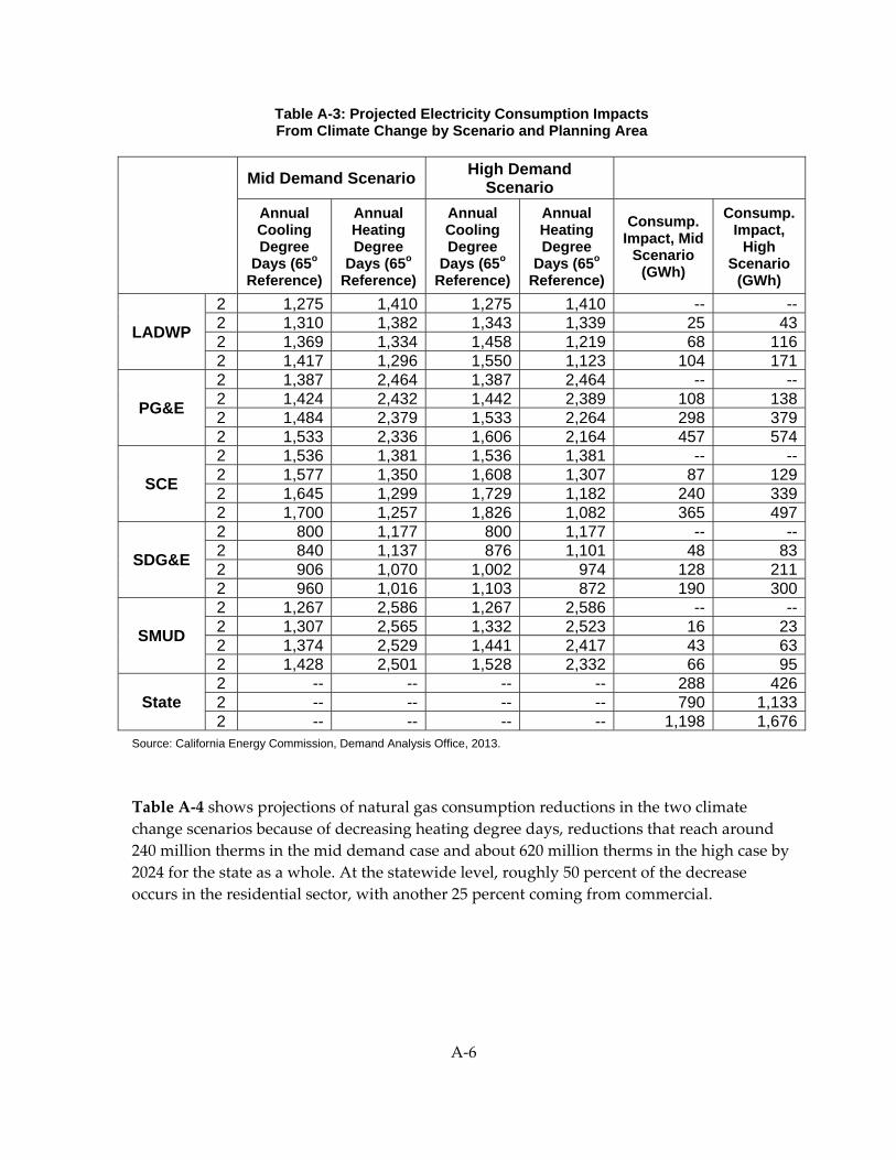
A‐6

Table A-3: Projected Electricity Consumption Impacts From Climate Change by Scenario and Planning Area

Mid Demand Scenario High Demand

Scenario

Annual Cooling Degree

Days (65o

Reference)

Annual Heating Degree

Days (65o

Reference)

Annual Cooling Degree

Days (65o

Reference)

Annual Heating Degree

Days (65o Reference)

Consump. Impact, Mid

Scenario (GWh)

Consump. Impact,

High Scenario

(GWh)

LADWP

2 1,275 1,410 1,275 1,410 -- --2 1,310 1,382 1,343 1,339 25 432 1,369 1,334 1,458 1,219 68 1162 1,417 1,296 1,550 1,123 104 171

PG&E

2 1,387 2,464 1,387 2,464 -- --2 1,424 2,432 1,442 2,389 108 1382 1,484 2,379 1,533 2,264 298 3792 1,533 2,336 1,606 2,164 457 574

SCE

2 1,536 1,381 1,536 1,381 -- --2 1,577 1,350 1,608 1,307 87 1292 1,645 1,299 1,729 1,182 240 3392 1,700 1,257 1,826 1,082 365 497

SDG&E

2 800 1,177 800 1,177 -- --2 840 1,137 876 1,101 48 832 906 1,070 1,002 974 128 2112 960 1,016 1,103 872 190 300

SMUD

2 1,267 2,586 1,267 2,586 -- --2 1,307 2,565 1,332 2,523 16 232 1,374 2,529 1,441 2,417 43 632 1,428 2,501 1,528 2,332 66 95

State 2 -- -- -- -- 288 4262 -- -- -- -- 790 1,1332 -- -- -- -- 1,198 1,676


Table A‐4 shows projections of natural gas consumption reductions in the two climate change scenarios because of decreasing heating degree days, reductions that reach around 240 million therms in the mid demand case and about 620 million therms in the high case by 2024 for the state as a whole. At the statewide level, roughly 50 percent of the decrease occurs in the residential sector, with another 25 percent coming from commercial.

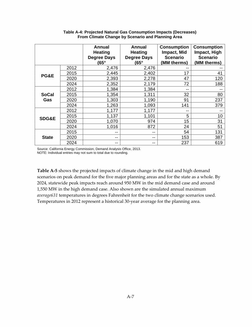
A‐7

Table A-4: Projected Natural Gas Consumption Impacts (Decreases) From Climate Change by Scenario and Planning Area

Annual Heating

Degree Days (65°

Annual Heating

Degree Days (65°

Consumption Impact, Mid

Scenario (MM therms)

Consumption Impact, High

Scenario (MM therms)

PG&E

2012 2,476 2,476 -- --2015 2,445 2,402 17 412020 2,393 2,278 47 1202024 2,352 2,179 72 188

SoCal Gas

2012 1,384 1,384 -- --2015 1,354 1,311 32 802020 1,303 1,190 91 2372024 1,263 1,093 141 379

SDG&E

2012 1,177 1,177 -- --2015 1,137 1,101 5 102020 1,070 974 15 312024 1,016 872 24 51

State 2015 -- -- 54 1312020 -- -- 153 3872024 -- -- 237 619

Source: California Energy Commission, Demand Analysis Office, 2013. NOTE: Individual entries may not sum to total due to rounding.

Table A‐5 shows the projected impacts of climate change in the mid and high demand scenarios on peak demand for the five major planning areas and for the state as a whole. By 2024, statewide peak impacts reach around 950 MW in the mid demand case and around 1,550 MW in the high demand case. Also shown are the simulated annual maximum average631 temperatures in degrees Fahrenheit for the two climate change scenarios used. Temperatures in 2012 represent a historical 30‐year average for the planning area.

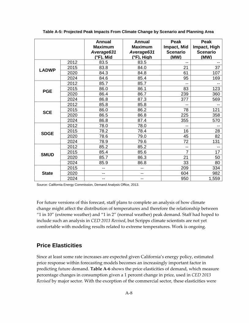
A‐8

Table A-5: Projected Peak Impacts From Climate Change by Scenario and Planning Area

Annual Maximum

Average631 (°F), Mid

Annual Maximum

Average631 (°F), High

Peak Impact, Mid

Scenario (MW)

Peak Impact, High

Scenario (MW)

LADWP

2012 83.5 83.5 -- --2015 83.8 84.0 21 372020 84.3 84.8 61 1072024 84.6 85.4 95 169

PGE

2012 85.7 85.7 -- --2015 86.0 86.1 83 1232020 86.4 86.7 239 3602024 86.8 87.3 377 569

SCE

2012 85.8 85.8 -- --2015 86.0 86.2 78 1212020 86.5 86.8 225 3582024 86.8 87.4 355 570

SDGE

2012 78.0 78.0 -- --2015 78.2 78.4 16 282020 78.6 79.0 45 822024 78.9 79.6 72 131

SMUD

2012 85.2 85.2 -- --2015 85.4 85.6 7 172020 85.7 86.3 21 502024 85.9 86.8 33 80

State 2015 -- -- 209 3342020 -- -- 604 9822024 -- -- 950 1,559


For future versions of this forecast, staff plans to complete an analysis of how climate change might affect the distribution of temperatures and therefore the relationship between “1 in 10” (extreme weather) and “1 in 2” (normal weather) peak demand. Staff had hoped to include such an analysis in CED 2013 Revised, but Scripps climate scientists are not yet comfortable with modeling results related to extreme temperatures. Work is ongoing.

Price Elasticities

Since at least some rate increases are expected given California’s energy policy, estimated price response within forecasting models becomes an increasingly important factor in predicting future demand. Table A‐6 shows the price elasticities of demand, which measure percentage changes in consumption given a 1 percent change in price, used in CED 2013 Revised by major sector. With the exception of the commercial sector, these elasticities were

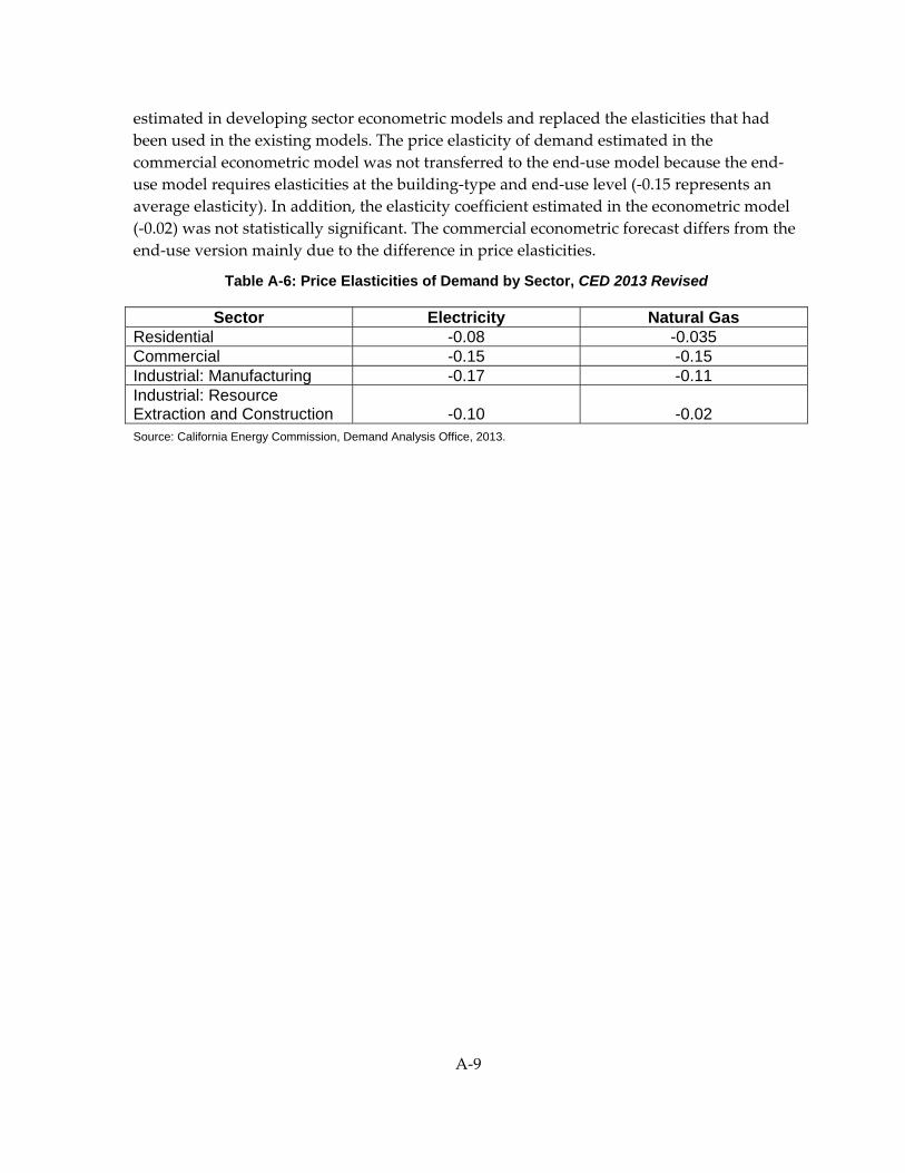
A‐9

estimated in developing sector econometric models and replaced the elasticities that had been used in the existing models. The price elasticity of demand estimated in the commercial econometric model was not transferred to the end‐use model because the end‐use model requires elasticities at the building‐type and end‐use level (‐0.15 represents an average elasticity). In addition, the elasticity coefficient estimated in the econometric model (‐0.02) was not statistically significant. The commercial econometric forecast differs from the end‐use version mainly due to the difference in price elasticities.

Table A-6: Price Elasticities of Demand by Sector, CED 2013 Revised

Sector Electricity Natural Gas Residential -0.08 -0.035 Commercial -0.15 -0.15 Industrial: Manufacturing -0.17 -0.11 Industrial: Resource Extraction and Construction -0.10 -0.02 Source: California Energy Commission, Demand Analysis Office, 2013.

B‐1

APPENDIX B: Self-Generation Forecasts

Compiling Historical Distributed Generation Data

The first stage of forecasting involved processing data from a variety of distributed generation (DG) incentive programs such as:

• The California Solar Initiative (CSI).71 • New Solar Homes Partnership (NSHP).72 • Self‐Generation Incentive Program (SGIP).73 • CSI Thermal Program for Solar Hot Water (SHW).74 • Emerging Renewables Program (ERP).75 • POU programs.76

In addition, power plants with a generating capacity of at least 1 MW are required to submit fuel use and generation data to the Energy Commission under the QFER Form 1304.77 QFER data include fuel use, generation, onsite use, and exports to the grid. These various sources of data were used to quantify DG activity in California and to build a comprehensive database to track DG activity. One concern in using incentive program data along with QFER data is the possibility of double‐counting generation if the project has a capacity of at least 1 MW. This can occur since the publicly available incentive program data do not list the name of the entity receiving the DG incentive for confidentially reasons while QFER data collects information from the plant owner. Therefore, it is not possible to determine if a

71 Downloaded on 6/19/13 from http://www.californiasolarstatistics.org/current_data_files/.

72 Program data received on 6/26/13 from staff in the Energy Commission’s Renewable Energy Office.

73 Downloaded on 06/24/13 from https://energycenter.org/index.php/incentive‐programs/self‐generation‐incentive‐program/sgip‐documents/sgip‐documents. Data cover up to first quarter of 2013.

74 Downloaded on 6/24/13 from http://www.gosolarcalifornia.org/solarwater/index.php.

75 Program data received on 1/18/13 from staff in the Commission’s Renewable Energy Office.

76 Program data submitted by POUs on June 2012 http://www.energy.ca.gov/sb1/pou_reports/index.html. Data covered additions occurring in 2011. Staff assumed that 2012 additions would be similar to 2011 since 2012 data will not be submitted to the Energy Commission until July 2013.

77 Data received from Energy Commission’s Electricity Analysis Office on 6/26/13.

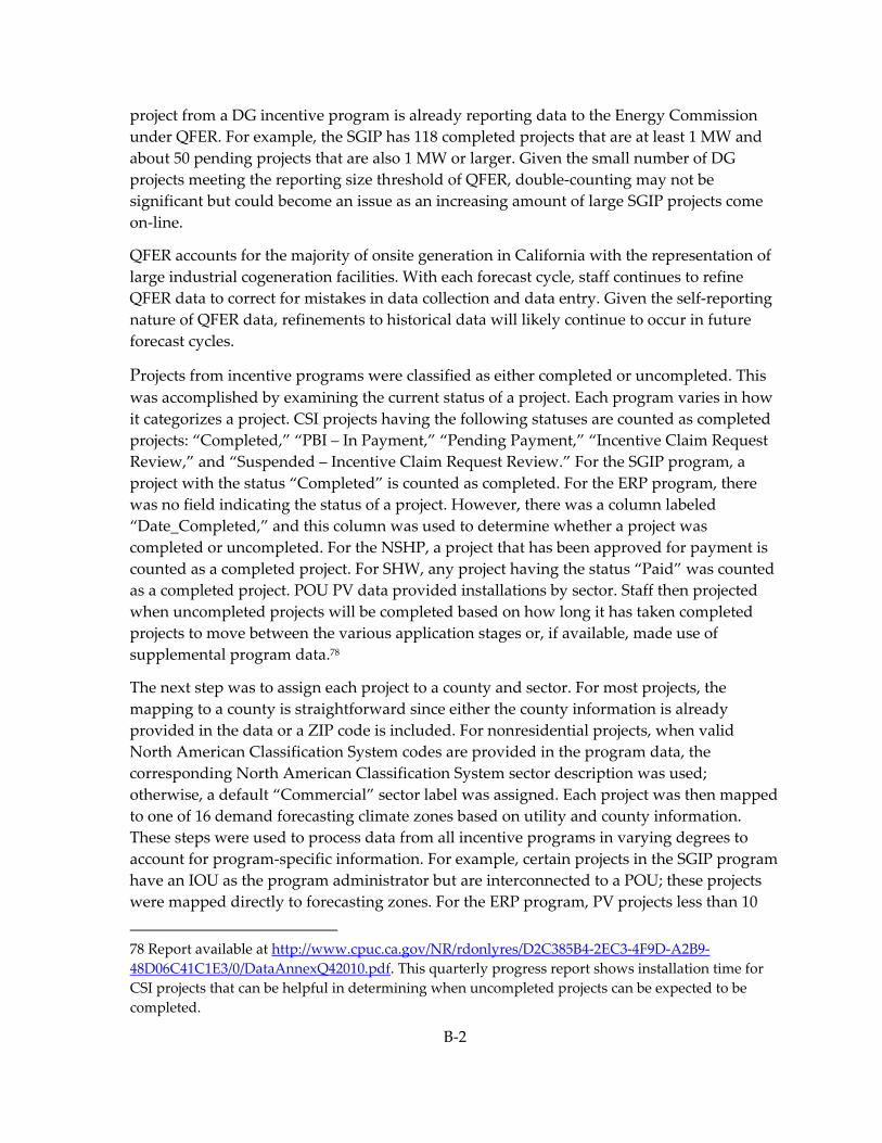
B‐2

project from a DG incentive program is already reporting data to the Energy Commission under QFER. For example, the SGIP has 118 completed projects that are at least 1 MW and about 50 pending projects that are also 1 MW or larger. Given the small number of DG projects meeting the reporting size threshold of QFER, double‐counting may not be significant but could become an issue as an increasing amount of large SGIP projects come on‐line.

QFER accounts for the majority of onsite generation in California with the representation of large industrial cogeneration facilities. With each forecast cycle, staff continues to refine QFER data to correct for mistakes in data collection and data entry. Given the self‐reporting nature of QFER data, refinements to historical data will likely continue to occur in future forecast cycles.

Projects from incentive programs were classified as either completed or uncompleted. This was accomplished by examining the current status of a project. Each program varies in how it categorizes a project. CSI projects having the following statuses are counted as completed projects: “Completed,” “PBI – In Payment,” “Pending Payment,” “Incentive Claim Request Review,” and “Suspended – Incentive Claim Request Review.” For the SGIP program, a project with the status “Completed” is counted as completed. For the ERP program, there was no field indicating the status of a project. However, there was a column labeled “Date_Completed,” and this column was used to determine whether a project was completed or uncompleted. For the NSHP, a project that has been approved for payment is counted as a completed project. For SHW, any project having the status “Paid” was counted as a completed project. POU PV data provided installations by sector. Staff then projected when uncompleted projects will be completed based on how long it has taken completed projects to move between the various application stages or, if available, made use of supplemental program data.78

The next step was to assign each project to a county and sector. For most projects, the mapping to a county is straightforward since either the county information is already provided in the data or a ZIP code is included. For nonresidential projects, when valid North American Classification System codes are provided in the program data, the corresponding North American Classification System sector description was used; otherwise, a default “Commercial” sector label was assigned. Each project was then mapped to one of 16 demand forecasting climate zones based on utility and county information. These steps were used to process data from all incentive programs in varying degrees to account for program‐specific information. For example, certain projects in the SGIP program have an IOU as the program administrator but are interconnected to a POU; these projects were mapped directly to forecasting zones. For the ERP program, PV projects less than 10

78 Report available at http://www.cpuc.ca.gov/NR/rdonlyres/D2C385B4‐2EC3‐4F9D‐A2B9‐48D06C41C1E3/0/DataAnnexQ42010.pdf. This quarterly progress report shows installation time for CSI projects that can be helpful in determining when uncompleted projects can be expected to be completed.

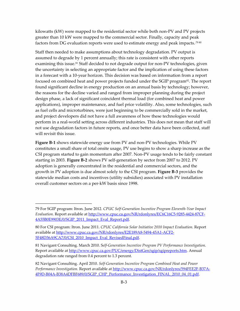
B‐3

kilowatts (kW) were mapped to the residential sector while both non‐PV and PV projects greater than 10 kW were mapped to the commercial sector. Finally, capacity and peak factors from DG evaluation reports were used to estimate energy and peak impacts..79 80

Staff then needed to make assumptions about technology degradation. PV output is assumed to degrade by 1 percent annually; this rate is consistent with other reports examining this issue.81 Staff decided to not degrade output for non‐PV technologies, given the uncertainty in selecting an appropriate factor and the implication of using these factors in a forecast with a 10‐year horizon. This decision was based on information from a report focused on combined heat and power projects funded under the SGIP program82. The report found significant decline in energy production on an annual basis by technology; however, the reasons for the decline varied and ranged from improper planning during the project design phase, a lack of significant coincident thermal load (for combined heat and power applications), improper maintenance, and fuel price volatility. Also, some technologies, such as fuel cells and microturbines, were just beginning to be commercially sold in the market, and project developers did not have a full awareness of how these technologies would perform in a real‐world setting across different industries. This does not mean that staff will not use degradation factors in future reports, and once better data have been collected, staff will revisit this issue.

Figure B‐1 shows statewide energy use from PV and non‐PV technologies. While PV constitutes a small share of total onsite usage, PV use begins to show a sharp increase as the CSI program started to gain momentum after 2007. Non‐PV usage tends to be fairly constant starting in 2003. Figure B‐2 shows PV self‐generation by sector from 2007 to 2012. PV adoption is generally concentrated in the residential and commercial sectors, and the growth in PV adoption is due almost solely to the CSI program. Figure B‐3 provides the statewide median costs and incentives (utility subsidies) associated with PV installation overall customer sectors on a per‐kW basis since 1998.

79 For SGIP program: Itron. June 2012. CPUC Self‐Generation Incentive Program Eleventh‐Year Impact Evaluation. Report available at http://www.cpuc.ca.gov/NR/rdonlyres/EC6C16C5‐9285‐4424‐87CF‐4A55B0E9903E/0/SGIP_2011_Impact_Eval_Report.pdf.

80 For CSI program: Itron. June 2011. CPUC California Solar Initiative 2010 Impact Evaluation. Report available at http://www.cpuc.ca.gov/NR/rdonlyres/E2E189A8‐5494‐45A1‐ACF2‐5F48D36A9CA7/0/CSI_2010_Impact_Eval_RevisedFinal.pdf.

81 Navigant Consulting. March 2010. Self‐Generation Incentive Program PV Performance Investigation. Report available at http://www.cpuc.ca.gov/PUC/energy/DistGen/sgip/sgipreports.htm. Annual degradation rate ranged from 0.4 percent to 1.3 percent.

82 Navigant Consulting. April 2010. Self‐Generation Incentive Program Combined Heat and Power Performance Investigation. Report available at http://www.cpuc.ca.gov/NR/rdonlyres/594FEE2F‐B37A‐4F9D‐B04A‐B38A4DFBF689/0/SGIP_CHP_Performance_Investigation_FINAL_2010_04_01.pdf.

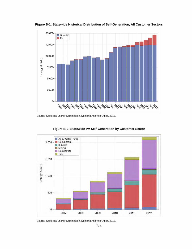
B‐4

Figure B-1: Statewide Historical Distribution of Self-Generation, All Customer Sectors


Figure B-2: Statewide PV Self-Generation by Customer Sector


B‐5

Figure B-3: Median PV Installation Costs and Subsidies, Statewide


For self‐generation as a whole, residential sector use is still a very small component of the total (around 5 percent in 2012). Figure B‐4 gives a breakout of self‐generation by nonresidential category for the state and shows a continued overall dominance by the industrial and mining (resource extraction) sectors, although commercial adoptions are clearly trending upward in recent years.

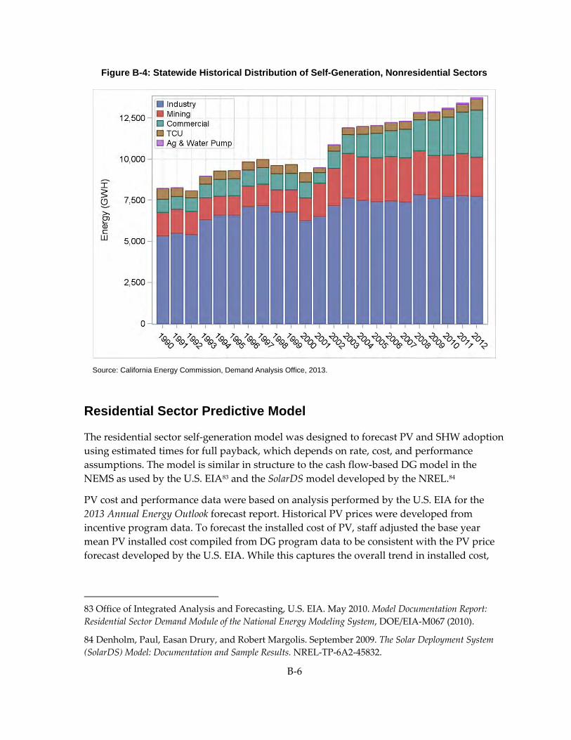
B‐6

Figure B-4: Statewide Historical Distribution of Self-Generation, Nonresidential Sectors


Residential Sector Predictive Model

The residential sector self‐generation model was designed to forecast PV and SHW adoption using estimated times for full payback, which depends on rate, cost, and performance assumptions. The model is similar in structure to the cash flow‐based DG model in the NEMS as used by the U.S. EIA83 and the SolarDS model developed by the NREL.84

PV cost and performance data were based on analysis performed by the U.S. EIA for the 2013 Annual Energy Outlook forecast report. Historical PV prices were developed from incentive program data. To forecast the installed cost of PV, staff adjusted the base year mean PV installed cost compiled from DG program data to be consistent with the PV price forecast developed by the U.S. EIA. While this captures the overall trend in installed cost,

83 Office of Integrated Analysis and Forecasting, U.S. EIA. May 2010. Model Documentation Report: Residential Sector Demand Module of the National Energy Modeling System, DOE/EIA‐M067 (2010).

84 Denholm, Paul, Easan Drury, and Robert Margolis. September 2009. The Solar Deployment System (SolarDS) Model: Documentation and Sample Results. NREL‐TP‐6A2‐45832.

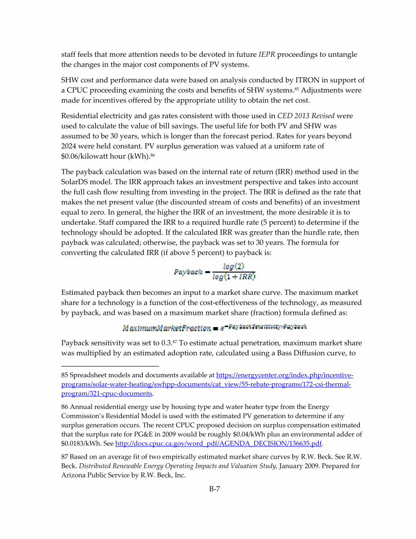
B‐7

staff feels that more attention needs to be devoted in future IEPR proceedings to untangle the changes in the major cost components of PV systems.

SHW cost and performance data were based on analysis conducted by ITRON in support of a CPUC proceeding examining the costs and benefits of SHW systems.85 Adjustments were made for incentives offered by the appropriate utility to obtain the net cost.

Residential electricity and gas rates consistent with those used in CED 2013 Revised were used to calculate the value of bill savings. The useful life for both PV and SHW was assumed to be 30 years, which is longer than the forecast period. Rates for years beyond 2024 were held constant. PV surplus generation was valued at a uniform rate of $0.06/kilowatt hour (kWh).86

The payback calculation was based on the internal rate of return (IRR) method used in the SolarDS model. The IRR approach takes an investment perspective and takes into account the full cash flow resulting from investing in the project. The IRR is defined as the rate that makes the net present value (the discounted stream of costs and benefits) of an investment equal to zero. In general, the higher the IRR of an investment, the more desirable it is to undertake. Staff compared the IRR to a required hurdle rate (5 percent) to determine if the technology should be adopted. If the calculated IRR was greater than the hurdle rate, then payback was calculated; otherwise, the payback was set to 30 years. The formula for converting the calculated IRR (if above 5 percent) to payback is:

Estimated payback then becomes an input to a market share curve. The maximum market share for a technology is a function of the cost‐effectiveness of the technology, as measured by payback, and was based on a maximum market share (fraction) formula defined as:

Payback sensitivity was set to 0.3.87 To estimate actual penetration, maximum market share was multiplied by an estimated adoption rate, calculated using a Bass Diffusion curve, to

85 Spreadsheet models and documents available at https://energycenter.org/index.php/incentive‐programs/solar‐water‐heating/swhpp‐documents/cat_view/55‐rebate‐programs/172‐csi‐thermal‐program/321‐cpuc‐documents.

86 Annual residential energy use by housing type and water heater type from the Energy Commission’s Residential Model is used with the estimated PV generation to determine if any surplus generation occurs. The recent CPUC proposed decision on surplus compensation estimated that the surplus rate for PG&E in 2009 would be roughly $0.04/kWh plus an environmental adder of $0.0183/kWh. See http://docs.cpuc.ca.gov/word_pdf/AGENDA_DECISION/136635.pdf.

87 Based on an average fit of two empirically estimated market share curves by R.W. Beck. See R.W. Beck. Distributed Renewable Energy Operating Impacts and Valuation Study, January 2009. Prepared for Arizona Public Service by R.W. Beck, Inc.

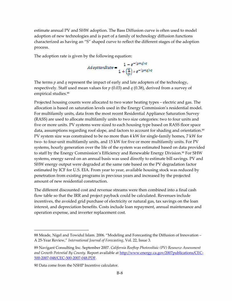
B‐8

estimate annual PV and SHW adoption. The Bass Diffusion curve is often used to model adoption of new technologies and is part of a family of technology diffusion functions characterized as having an “S” shaped curve to reflect the different stages of the adoption process.

The adoption rate is given by the following equation:

The terms p and q represent the impact of early and late adopters of the technology, respectively. Staff used mean values for p (0.03) and q (0.38), derived from a survey of empirical studies.88

Projected housing counts were allocated to two water heating types – electric and gas. The allocation is based on saturation levels used in the Energy Commission’s residential model. For multifamily units, data from the most recent Residential Appliance Saturation Survey (RASS) are used to allocate multifamily units to two size categories: two to four units and five or more units. PV systems were sized to each housing type based on RASS floor space data, assumptions regarding roof slope, and factors to account for shading and orientation.89 PV system size was constrained to be no more than 4 kW for single‐family homes, 7 kW for two‐ to four‐unit multifamily units, and 15 kW for five or more multifamily units. For PV systems, hourly generation over the life of the system was estimated based on data provided to staff by the Energy Commission’s Efficiency and Renewable Energy Division.90 For SHW systems, energy saved on an annual basis was used directly to estimate bill savings. PV and SHW energy output were degraded at the same rate based on the PV degradation factor estimated by ICF for U.S. EIA. From year to year, available housing stock was reduced by penetration from existing programs in previous years and increased by the projected amount of new residential construction.

The different discounted cost and revenue streams were then combined into a final cash flow table so that the IRR and project payback could be calculated. Revenues include incentives, the avoided grid purchase of electricity or natural gas, tax savings on the loan interest, and depreciation benefits. Costs include loan repayment, annual maintenance and operation expense, and inverter replacement cost.

88 Meade, Nigel and Towidul Islam. 2006. “Modeling and Forecasting the Diffusion of Innovation – A 25‐Year Review,” International Journal of Forecasting, Vol. 22, Issue 3.

89 Navigant Consulting Inc. September 2007. California Rooftop Photovoltaic (PV) Resource Assessment and Growth Potential By County. Report available at http://www.energy.ca.gov/2007publications/CEC‐500‐2007‐048/CEC‐500‐2007‐048.PDF.

90 Data come from the NSHP Incentive calculator.

B‐9

Self-Generation Forecast, Nonresidential Sectors

Commercial CHP and PV Forecast CED 2013 Preliminary incorporated a newly developed predictive model for commercial CHP. CED 2013 Revised incorporates within the same model a predictive framework for commercial PV adoption. The model uses the same basic payback framework as in the residential predictive model. Staff began by allocating energy use to different building types using the 2006 Commercial End‐Use Survey (CEUS).91 The survey contains information on each site that participated in the survey, including:

• Site floor space.

• Site roof area.

• Electricity and natural gas use per square foot.

• Grouping variables and weights for building type, building size, and forecasting climate zone.

Building sizes were grouped into four size categories based on annual electricity use. Fuel intensities (use per square foot) were then calculated for each building type and size for electricity and natural gas.

Next, the “DrCEUS” building energy use simulation tool, developed in conjunction with the CEUS, was used to create load shapes by fuel type and end use. DrCEUS uses the eQUEST building energy use software tool as a “front end” to the considerably more complex Department of Energy DOE 2.2 building energy use simulation tool, which does much of the actual building energy demand simulation.

Staff grouped small and medium‐size buildings together since the CEUS survey had a limited number of sample points for these building sizes. In addition, because of small sample sizes, staff grouped inland and coastal climate zones together. Four geographic profiles were created: north inland, north coastal, south inland, and south coastal. These profiles were used to create prototypical building energy use load profiles that could then be used to assess the suitability of different CHP technologies in meeting onsite demand for heat and power. As examples, Figure B‐5 shows the distribution of annual consumption among end uses for electricity and natural gas for the north coastal climate zones for small/medium‐size buildings, and Figure B‐6 shows hourly electricity loads for south coastal large schools.

91 Itron. March 2006. Report available at http://www.energy.ca.gov/2006publications/CEC‐400‐2006‐005/CEC‐400‐2006‐005.PDF.

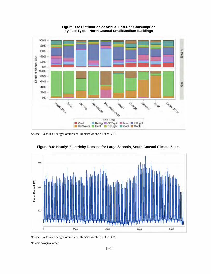
B‐10

Figure B-5: Distribution of Annual End-Use Consumption by Fuel Type – North Coastal Small/Medium Buildings


Figure B-6: Hourly* Electricity Demand for Large Schools, South Coastal Climate Zones


*In chronological order.

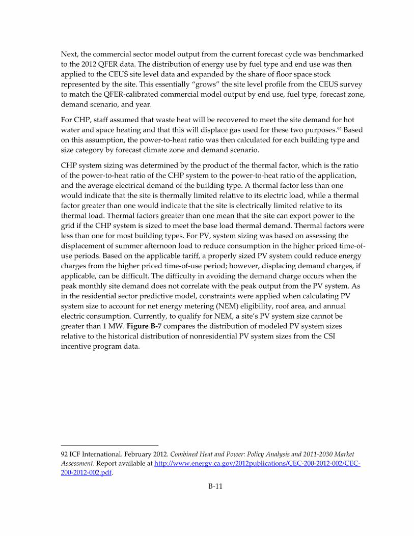
B‐11

Next, the commercial sector model output from the current forecast cycle was benchmarked to the 2012 QFER data. The distribution of energy use by fuel type and end use was then applied to the CEUS site level data and expanded by the share of floor space stock represented by the site. This essentially “grows” the site level profile from the CEUS survey to match the QFER‐calibrated commercial model output by end use, fuel type, forecast zone, demand scenario, and year.

For CHP, staff assumed that waste heat will be recovered to meet the site demand for hot water and space heating and that this will displace gas used for these two purposes.92 Based on this assumption, the power‐to‐heat ratio was then calculated for each building type and size category by forecast climate zone and demand scenario.

CHP system sizing was determined by the product of the thermal factor, which is the ratio of the power‐to‐heat ratio of the CHP system to the power‐to‐heat ratio of the application, and the average electrical demand of the building type. A thermal factor less than one would indicate that the site is thermally limited relative to its electric load, while a thermal factor greater than one would indicate that the site is electrically limited relative to its thermal load. Thermal factors greater than one mean that the site can export power to the grid if the CHP system is sized to meet the base load thermal demand. Thermal factors were less than one for most building types. For PV, system sizing was based on assessing the displacement of summer afternoon load to reduce consumption in the higher priced time‐of‐use periods. Based on the applicable tariff, a properly sized PV system could reduce energy charges from the higher priced time‐of‐use period; however, displacing demand charges, if applicable, can be difficult. The difficulty in avoiding the demand charge occurs when the peak monthly site demand does not correlate with the peak output from the PV system. As in the residential sector predictive model, constraints were applied when calculating PV system size to account for net energy metering (NEM) eligibility, roof area, and annual electric consumption. Currently, to qualify for NEM, a site’s PV system size cannot be greater than 1 MW. Figure B‐7 compares the distribution of modeled PV system sizes relative to the historical distribution of nonresidential PV system sizes from the CSI incentive program data.

92 ICF International. February 2012. Combined Heat and Power: Policy Analysis and 2011‐2030 Market Assessment. Report available at http://www.energy.ca.gov/2012publications/CEC‐200‐2012‐002/CEC‐200‐2012‐002.pdf.

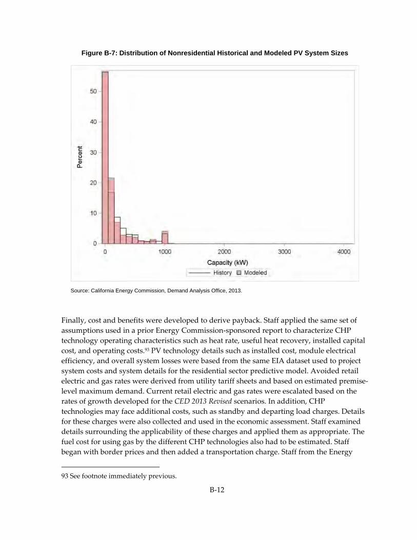
B‐12

Figure B-7: Distribution of Nonresidential Historical and Modeled PV System Sizes


Finally, cost and benefits were developed to derive payback. Staff applied the same set of assumptions used in a prior Energy Commission‐sponsored report to characterize CHP technology operating characteristics such as heat rate, useful heat recovery, installed capital cost, and operating costs.93 PV technology details such as installed cost, module electrical efficiency, and overall system losses were based from the same EIA dataset used to project system costs and system details for the residential sector predictive model. Avoided retail electric and gas rates were derived from utility tariff sheets and based on estimated premise‐level maximum demand. Current retail electric and gas rates were escalated based on the rates of growth developed for the CED 2013 Revised scenarios. In addition, CHP technologies may face additional costs, such as standby and departing load charges. Details for these charges were also collected and used in the economic assessment. Staff examined details surrounding the applicability of these charges and applied them as appropriate. The fuel cost for using gas by the different CHP technologies also had to be estimated. Staff began with border prices and then added a transportation charge. Staff from the Energy

93 See footnote immediately previous.

B‐13

Commission’s Electricity Analysis Office supplied the historical border prices. The Malin border price was used for PG&E, and the Southern California border price was used for both SoCal Gas and SDG&E. For the forecast period, staff escalated average 2012 border prices at a rate consistent with the Electricity Analysis Office’s gas rate scenarios.94 Staff also identified federal tax credits for installing CHP and PV and assessed the eligibility for utility rebate programs, such as the SGIP and CSI.

The cash flow analysis and payback based adoption modeling were performed similarly to the residential sector PV model process, described earlier.

Other Sector Self-Generation Staff used a trend analysis for forecasting adoption of PV in the noncommercial/nonresidential sectors. Using CSI incentive program data, staff calculated the average annual growth rate for each sector and forecast climate zone for 2008 – 2012. Given strong growth for PV adoption in this period, the maximum annual growth rate was capped at 12 percent. Installed capacity was allowed to grow at this rate until 2016, when the growth rate was reduced by half to account for expiration of federal tax credits. For SHW, staff assumed that nonresidential sector adoption would follow a ratio similar to residential versus nonresidential PV adoption.

Statewide Modeling Results The following figures show results from the three predictive models at the statewide level by demand scenario. Figure B‐8 shows the PV peak demand impact in the residential sector, which reaches more than 800 MW in the mid demand case and around 1,100 MW in the low case by 2024. Potential adoptions were limited to owner‐occupied households, meaning that model results were reduced by percentage of home rentals in each planning area derived from RASS data. For future forecasting cycles, staff will attempt to analyze potential adoption in rental properties separately. Additions decrease substantially with the expiration of the federal tax credit, which occurs in the middle of the forecast period, but then begin to increase as rates increase and PV installed costs decrease.

94 Brathwaite, Leon, Paul Deaver, Robert Kennedy, et al. 2011 Natural Gas Market Assessment: Outlook. May 2012. Report available at (http://www.energy.ca.gov/2011publications/CEC‐200‐2011‐012/CEC‐200‐2011‐012‐SF.pdf). The 2012 daily rates come from Natural Gas Intelligence and were supplied by staff from Electricity Analysis Office.

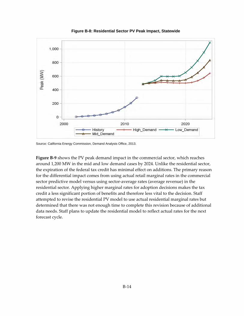
B‐14

Figure B-8: Residential Sector PV Peak Impact, Statewide


Figure B‐9 shows the PV peak demand impact in the commercial sector, which reaches around 1,200 MW in the mid and low demand cases by 2024. Unlike the residential sector, the expiration of the federal tax credit has minimal effect on additions. The primary reason for the differential impact comes from using actual retail marginal rates in the commercial sector predictive model versus using sector‐average rates (average revenue) in the residential sector. Applying higher marginal rates for adoption decisions makes the tax credit a less significant portion of benefits and therefore less vital to the decision. Staff attempted to revise the residential PV model to use actual residential marginal rates but determined that there was not enough time to complete this revision because of additional data needs. Staff plans to update the residential model to reflect actual rates for the next forecast cycle.

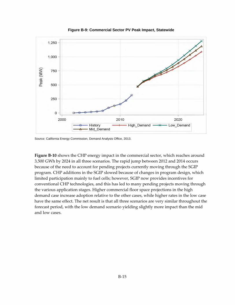
B‐15

Figure B-9: Commercial Sector PV Peak Impact, Statewide


Figure B‐10 shows the CHP energy impact in the commercial sector, which reaches around 3,500 GWh by 2024 in all three scenarios. The rapid jump between 2012 and 2014 occurs because of the need to account for pending projects currently moving through the SGIP program. CHP additions in the SGIP slowed because of changes in program design, which limited participation mainly to fuel cells; however, SGIP now provides incentives for conventional CHP technologies, and this has led to many pending projects moving through the various application stages. Higher commercial floor space projections in the high demand case increase adoption relative to the other cases, while higher rates in the low case have the same effect. The net result is that all three scenarios are very similar throughout the forecast period, with the low demand scenario yielding slightly more impact than the mid and low cases.

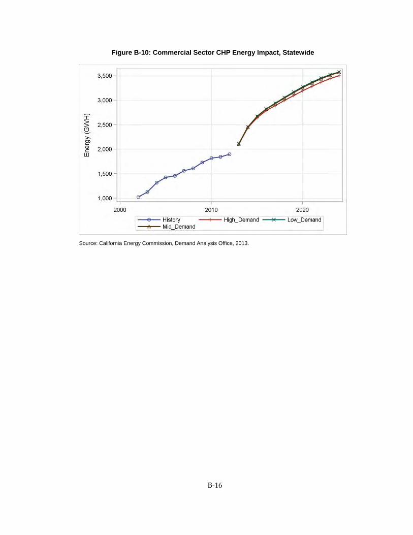
B‐16

Figure B-10: Commercial Sector CHP Energy Impact, Statewide


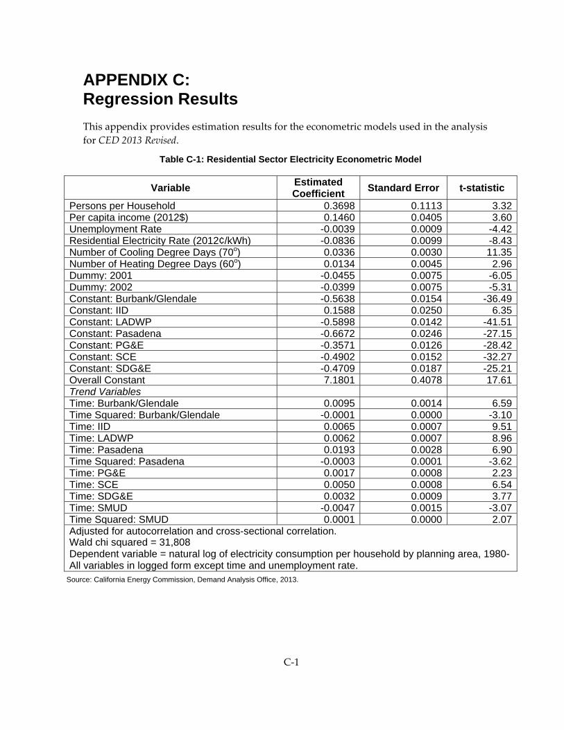
C‐1

APPENDIX C: Regression Results This appendix provides estimation results for the econometric models used in the analysis for CED 2013 Revised.

Table C-1: Residential Sector Electricity Econometric Model

Variable Estimated Coefficient Standard Error t-statistic

Persons per Household 0.3698 0.1113 3.32Per capita income (2012$) 0.1460 0.0405 3.60Unemployment Rate -0.0039 0.0009 -4.42Residential Electricity Rate (2012¢/kWh) -0.0836 0.0099 -8.43Number of Cooling Degree Days (70o) 0.0336 0.0030 11.35Number of Heating Degree Days (60o) 0.0134 0.0045 2.96Dummy: 2001 -0.0455 0.0075 -6.05Dummy: 2002 -0.0399 0.0075 -5.31Constant: Burbank/Glendale -0.5638 0.0154 -36.49Constant: IID 0.1588 0.0250 6.35Constant: LADWP -0.5898 0.0142 -41.51Constant: Pasadena -0.6672 0.0246 -27.15Constant: PG&E -0.3571 0.0126 -28.42Constant: SCE -0.4902 0.0152 -32.27Constant: SDG&E -0.4709 0.0187 -25.21Overall Constant 7.1801 0.4078 17.61Trend Variables Time: Burbank/Glendale 0.0095 0.0014 6.59Time Squared: Burbank/Glendale -0.0001 0.0000 -3.10Time: IID 0.0065 0.0007 9.51Time: LADWP 0.0062 0.0007 8.96Time: Pasadena 0.0193 0.0028 6.90Time Squared: Pasadena -0.0003 0.0001 -3.62Time: PG&E 0.0017 0.0008 2.23Time: SCE 0.0050 0.0008 6.54Time: SDG&E 0.0032 0.0009 3.77Time: SMUD -0.0047 0.0015 -3.07Time Squared: SMUD 0.0001 0.0000 2.07Adjusted for autocorrelation and cross-sectional correlation.Wald chi squared = 31,808 Dependent variable = natural log of electricity consumption per household by planning area, 1980-All variables in logged form except time and unemployment rate.


C‐2

Table C-2: Commercial Sector Electricity Econometric Model

Variable Estimated Coefficient

Standard Error t-statistic

Commercial Floor Space (mm. sq. ft.) 0.8682 0.0658 13.19% of Floor Space Refrigerated 0.2931 0.0364 8.06Commercial Employment/Floor Space 0.4662 0.0788 5.92Personal Income (billion 2012$) 0.1437 0.0588 2.44Commercial Electricity Rate (2012¢/kWh) -0.0173 0.0147 -1.18Natural Gas Rate: except SMUD (2012$/mm. 0.0109 0.0072 1.52Number of Cooling Degree Days (65o) 0.0470 0.0083 5.64Dummy: 2001 (LADWP) -0.0445 0.0196 -2.27Dummy: 2001 (PG&E) -0.0340 0.0148 -2.30Dummy: 2001 (SDG&E -0.0709 0.0177 -4.00Constant: IID 0.1110 0.0442 2.51Constant: LADWP -0.1214 0.0339 -3.58Constant: Pasadena 0.3863 0.0787 4.91Constant: PG&E -0.2973 0.0624 -4.76Constant: SCE -0.3012 0.0616 -4.89Overall Constant 2.0984 0.2001 10.49Trend Variables Time 0.0086 0.0017 4.97Time Squared -0.0002 0.0000 -5.49Additional Time Impact: Burbank/Glendale 0.0295 0.0036 8.13Additional Time Squared Impact: -0.0006 0.0001 -6.39Additional Time Impact: IID 0.0151 0.0030 5.10Additional Time Squared Impact: IID -0.0003 0.0001 -3.55Additional Time Impact: Pasadena 0.0068 0.0038 1.78Additional Time Impact: SCE 0.0036 0.0006 5.81Adjusted for autocorrelation and cross-sectional correlation. Wald chi squared = 378,145 Dependent variable = natural log of commercial consumption by planning area, 1980-2012. All variables in logged form except time and % of floor space refrigerated.


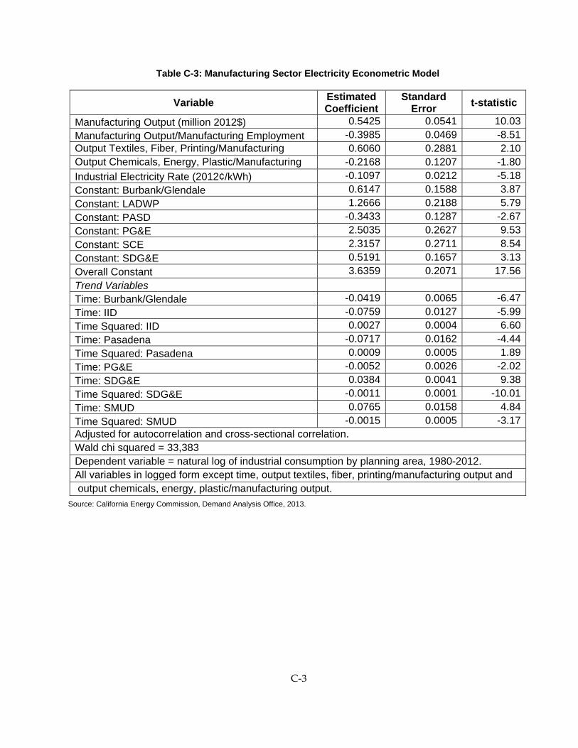
C‐3

Table C-3: Manufacturing Sector Electricity Econometric Model



Manufacturing Output (million 2012$) 0.5425 0.0541 10.03Manufacturing Output/Manufacturing Employment -0.3985 0.0469 -8.51Output Textiles, Fiber, Printing/Manufacturing 0.6060 0.2881 2.10Output Chemicals, Energy, Plastic/Manufacturing -0.2168 0.1207 -1.80Industrial Electricity Rate (2012¢/kWh) -0.1097 0.0212 -5.18Constant: Burbank/Glendale 0.6147 0.1588 3.87Constant: LADWP 1.2666 0.2188 5.79Constant: PASD -0.3433 0.1287 -2.67Constant: PG&E 2.5035 0.2627 9.53Constant: SCE 2.3157 0.2711 8.54Constant: SDG&E 0.5191 0.1657 3.13Overall Constant 3.6359 0.2071 17.56Trend Variables Time: Burbank/Glendale -0.0419 0.0065 -6.47Time: IID -0.0759 0.0127 -5.99Time Squared: IID 0.0027 0.0004 6.60Time: Pasadena -0.0717 0.0162 -4.44Time Squared: Pasadena 0.0009 0.0005 1.89Time: PG&E -0.0052 0.0026 -2.02Time: SDG&E 0.0384 0.0041 9.38Time Squared: SDG&E -0.0011 0.0001 -10.01Time: SMUD 0.0765 0.0158 4.84Time Squared: SMUD -0.0015 0.0005 -3.17Adjusted for autocorrelation and cross-sectional correlation. Wald chi squared = 33,383 Dependent variable = natural log of industrial consumption by planning area, 1980-2012. All variables in logged form except time, output textiles, fiber, printing/manufacturing output and output chemicals, energy, plastic/manufacturing output.


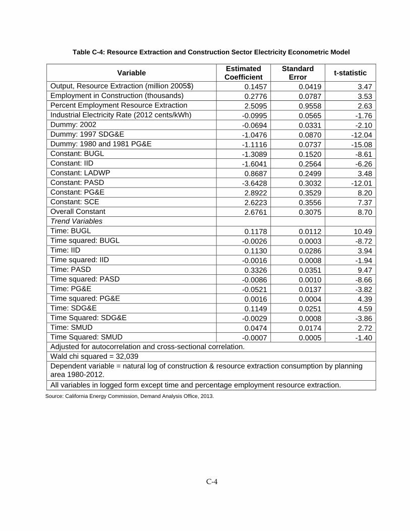
C‐4

Table C-4: Resource Extraction and Construction Sector Electricity Econometric Model



Output, Resource Extraction (million 2005$) 0.1457 0.0419 3.47Employment in Construction (thousands) 0.2776 0.0787 3.53Percent Employment Resource Extraction 2.5095 0.9558 2.63Industrial Electricity Rate (2012 cents/kWh) -0.0995 0.0565 -1.76Dummy: 2002 -0.0694 0.0331 -2.10Dummy: 1997 SDG&E -1.0476 0.0870 -12.04Dummy: 1980 and 1981 PG&E -1.1116 0.0737 -15.08Constant: BUGL -1.3089 0.1520 -8.61Constant: IID -1.6041 0.2564 -6.26Constant: LADWP 0.8687 0.2499 3.48Constant: PASD -3.6428 0.3032 -12.01Constant: PG&E 2.8922 0.3529 8.20Constant: SCE 2.6223 0.3556 7.37Overall Constant 2.6761 0.3075 8.70Trend Variables Time: BUGL 0.1178 0.0112 10.49Time squared: BUGL -0.0026 0.0003 -8.72Time: IID 0.1130 0.0286 3.94Time squared: IID -0.0016 0.0008 -1.94Time: PASD 0.3326 0.0351 9.47Time squared: PASD -0.0086 0.0010 -8.66Time: PG&E -0.0521 0.0137 -3.82Time squared: PG&E 0.0016 0.0004 4.39Time: SDG&E 0.1149 0.0251 4.59Time Squared: SDG&E -0.0029 0.0008 -3.86Time: SMUD 0.0474 0.0174 2.72Time Squared: SMUD -0.0007 0.0005 -1.40Adjusted for autocorrelation and cross-sectional correlation. Wald chi squared = 32,039 Dependent variable = natural log of construction & resource extraction consumption by planning area 1980-2012. All variables in logged form except time and percentage employment resource extraction.


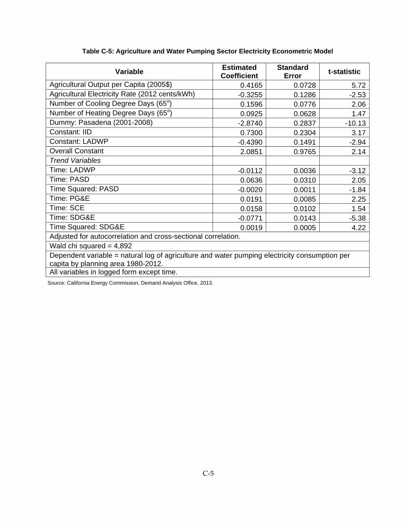
C‐5

Table C-5: Agriculture and Water Pumping Sector Electricity Econometric Model



Agricultural Output per Capita (2005$) 0.4165 0.0728 5.72Agricultural Electricity Rate (2012 cents/kWh) -0.3255 0.1286 -2.53Number of Cooling Degree Days (65o) 0.1596 0.0776 2.06Number of Heating Degree Days (65o) 0.0925 0.0628 1.47Dummy: Pasadena (2001-2008) -2.8740 0.2837 -10.13Constant: IID 0.7300 0.2304 3.17Constant: LADWP -0.4390 0.1491 -2.94Overall Constant 2.0851 0.9765 2.14Trend Variables Time: LADWP -0.0112 0.0036 -3.12Time: PASD 0.0636 0.0310 2.05Time Squared: PASD -0.0020 0.0011 -1.84Time: PG&E 0.0191 0.0085 2.25Time: SCE 0.0158 0.0102 1.54Time: SDG&E -0.0771 0.0143 -5.38Time Squared: SDG&E 0.0019 0.0005 4.22Adjusted for autocorrelation and cross-sectional correlation. Wald chi squared = 4,892 Dependent variable = natural log of agriculture and water pumping electricity consumption per capita by planning area 1980-2012.All variables in logged form except time.


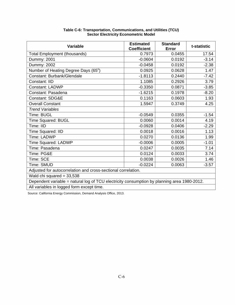
C‐6

Table C-6: Transportation, Communications, and Utilities (TCU) Sector Electricity Econometric Model



Total Employment (thousands) 0.7973 0.0455 17.54Dummy: 2001 -0.0604 0.0192 -3.14Dummy: 2002 -0.0458 0.0192 -2.38Number of Heating Degree Days (65o) 0.0925 0.0628 1.47Constant: Burbank/Glendale -1.8113 0.2440 -7.42Constant: IID 1.1085 0.2926 3.79Constant: LADWP -0.3350 0.0871 -3.85Constant: Pasadena -1.6215 0.1978 -8.20Constant: SDG&E 0.1163 0.0603 1.93Overall Constant 1.5947 0.3749 4.25Trend Variables Time: BUGL -0.0549 0.0355 -1.54Time Squared: BUGL 0.0060 0.0014 4.19Time: IID -0.0928 0.0406 -2.29Time Squared: IID 0.0018 0.0016 1.13Time: LADWP 0.0270 0.0136 1.99Time Squared: LADWP -0.0006 0.0005 -1.01Time: Pasadena 0.0247 0.0035 7.14Time: PG&E 0.0124 0.0033 3.74Time: SCE 0.0038 0.0026 1.46Time: SMUD -0.0224 0.0063 -3.57Adjusted for autocorrelation and cross-sectional correlation. Wald chi squared = 33,538 Dependent variable = natural log of TCU electricity consumption by planning area 1980-2012. All variables in logged form except time.


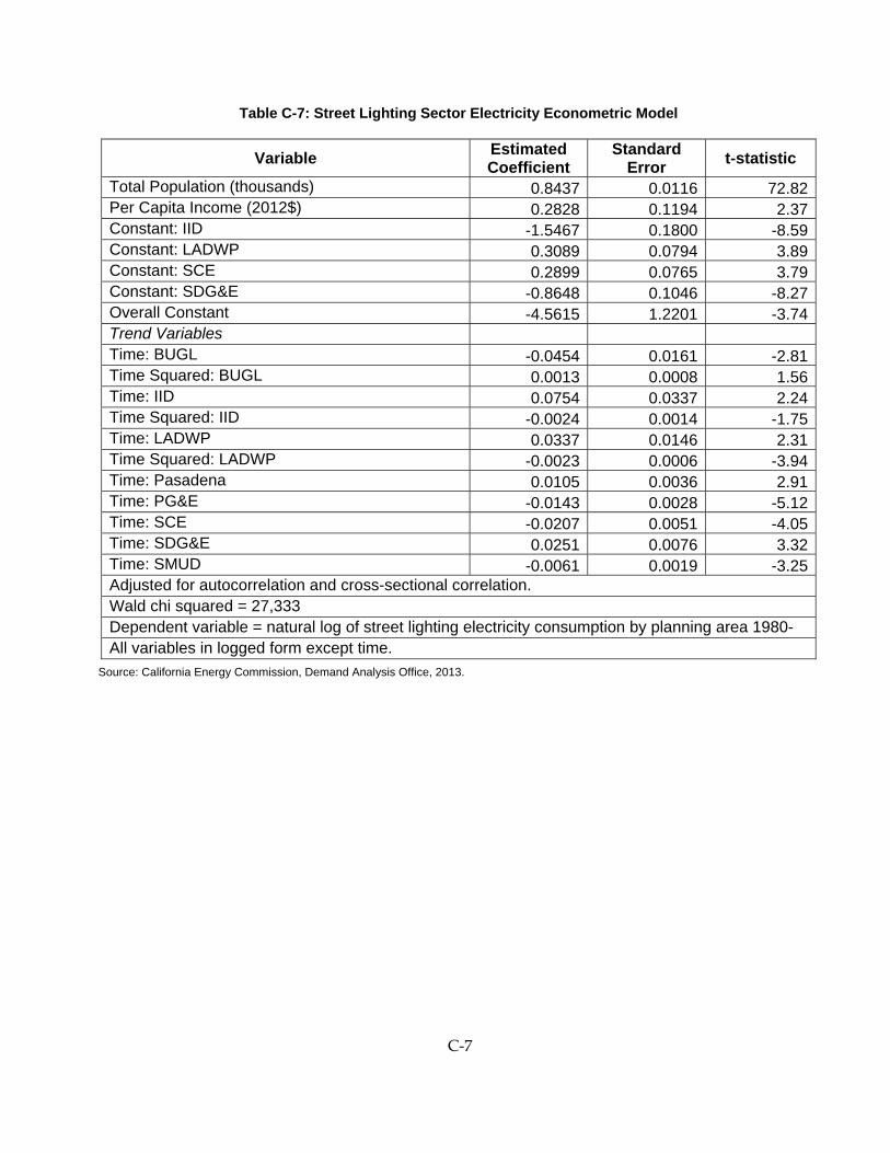
C‐7

Table C-7: Street Lighting Sector Electricity Econometric Model



Total Population (thousands) 0.8437 0.0116 72.82Per Capita Income (2012$) 0.2828 0.1194 2.37Constant: IID -1.5467 0.1800 -8.59Constant: LADWP 0.3089 0.0794 3.89Constant: SCE 0.2899 0.0765 3.79Constant: SDG&E -0.8648 0.1046 -8.27Overall Constant -4.5615 1.2201 -3.74Trend Variables Time: BUGL -0.0454 0.0161 -2.81Time Squared: BUGL 0.0013 0.0008 1.56Time: IID 0.0754 0.0337 2.24Time Squared: IID -0.0024 0.0014 -1.75Time: LADWP 0.0337 0.0146 2.31Time Squared: LADWP -0.0023 0.0006 -3.94Time: Pasadena 0.0105 0.0036 2.91Time: PG&E -0.0143 0.0028 -5.12Time: SCE -0.0207 0.0051 -4.05Time: SDG&E 0.0251 0.0076 3.32Time: SMUD -0.0061 0.0019 -3.25Adjusted for autocorrelation and cross-sectional correlation. Wald chi squared = 27,333 Dependent variable = natural log of street lighting electricity consumption by planning area 1980-All variables in logged form except time.


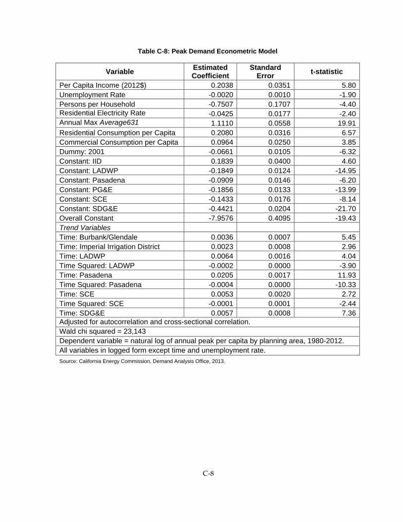
C‐8

Table C-8: Peak Demand Econometric Model



Per Capita Income (2012$) 0.2038 0.0351 5.80Unemployment Rate -0.0020 0.0010 -1.90Persons per Household -0.7507 0.1707 -4.40Residential Electricity Rate -0.0425 0.0177 -2.40Annual Max Average631 1.1110 0.0558 19.91Residential Consumption per Capita 0.2080 0.0316 6.57Commercial Consumption per Capita 0.0964 0.0250 3.85Dummy: 2001 -0.0661 0.0105 -6.32Constant: IID 0.1839 0.0400 4.60Constant: LADWP -0.1849 0.0124 -14.95Constant: Pasadena -0.0909 0.0146 -6.20Constant: PG&E -0.1856 0.0133 -13.99Constant: SCE -0.1433 0.0176 -8.14Constant: SDG&E -0.4421 0.0204 -21.70Overall Constant -7.9576 0.4095 -19.43Trend Variables Time: Burbank/Glendale 0.0036 0.0007 5.45Time: Imperial Irrigation District 0.0023 0.0008 2.96Time: LADWP 0.0064 0.0016 4.04Time Squared: LADWP -0.0002 0.0000 -3.90Time: Pasadena 0.0205 0.0017 11.93Time Squared: Pasadena -0.0004 0.0000 -10.33Time: SCE 0.0053 0.0020 2.72Time Squared: SCE -0.0001 0.0001 -2.44Time: SDG&E 0.0057 0.0008 7.36Adjusted for autocorrelation and cross-sectional correlation. Wald chi squared = 23,143 Dependent variable = natural log of annual peak per capita by planning area, 1980-2012. All variables in logged form except time and unemployment rate. Source: California Energy Commission, Demand Analysis Office, 2013.

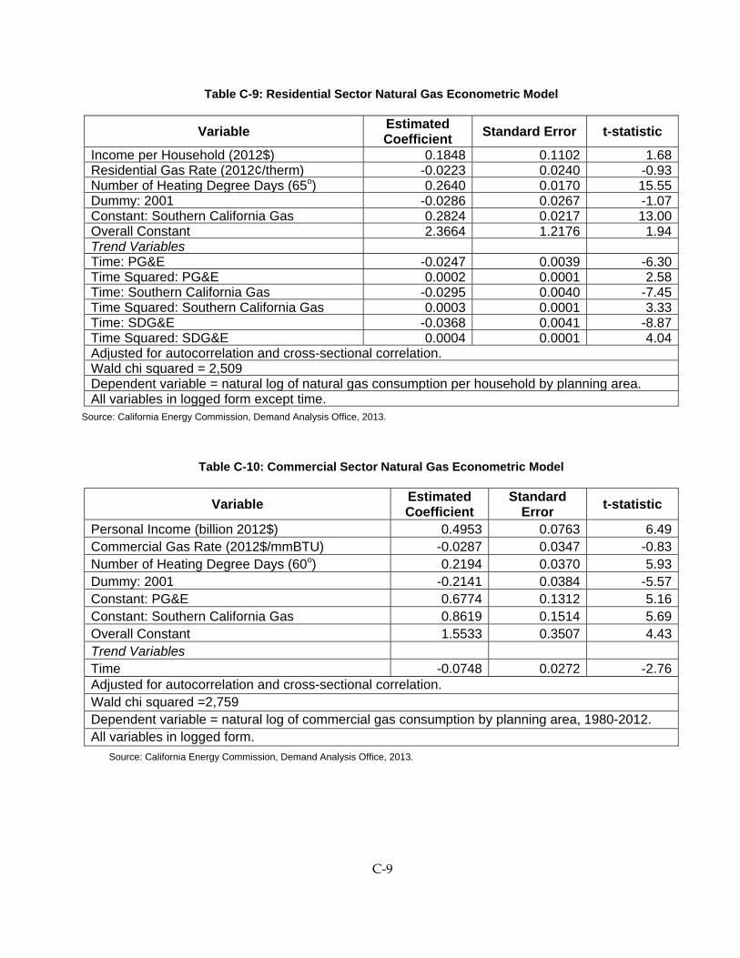
C‐9

Table C-9: Residential Sector Natural Gas Econometric Model

Variable Estimated Coefficient Standard Error t-statistic

Income per Household (2012$) 0.1848 0.1102 1.68Residential Gas Rate (2012¢/therm) -0.0223 0.0240 -0.93Number of Heating Degree Days (65o) 0.2640 0.0170 15.55Dummy: 2001 -0.0286 0.0267 -1.07Constant: Southern California Gas 0.2824 0.0217 13.00Overall Constant 2.3664 1.2176 1.94Trend Variables Time: PG&E -0.0247 0.0039 -6.30Time Squared: PG&E 0.0002 0.0001 2.58Time: Southern California Gas -0.0295 0.0040 -7.45Time Squared: Southern California Gas 0.0003 0.0001 3.33Time: SDG&E -0.0368 0.0041 -8.87Time Squared: SDG&E 0.0004 0.0001 4.04Adjusted for autocorrelation and cross-sectional correlation.Wald chi squared = 2,509 Dependent variable = natural log of natural gas consumption per household by planning area.All variables in logged form except time.


Table C-10: Commercial Sector Natural Gas Econometric Model



Personal Income (billion 2012$) 0.4953 0.0763 6.49Commercial Gas Rate (2012$/mmBTU) -0.0287 0.0347 -0.83Number of Heating Degree Days (60o) 0.2194 0.0370 5.93Dummy: 2001 -0.2141 0.0384 -5.57Constant: PG&E 0.6774 0.1312 5.16Constant: Southern California Gas 0.8619 0.1514 5.69Overall Constant 1.5533 0.3507 4.43Trend Variables Time -0.0748 0.0272 -2.76Adjusted for autocorrelation and cross-sectional correlation. Wald chi squared =2,759 Dependent variable = natural log of commercial gas consumption by planning area, 1980-2012. All variables in logged form.


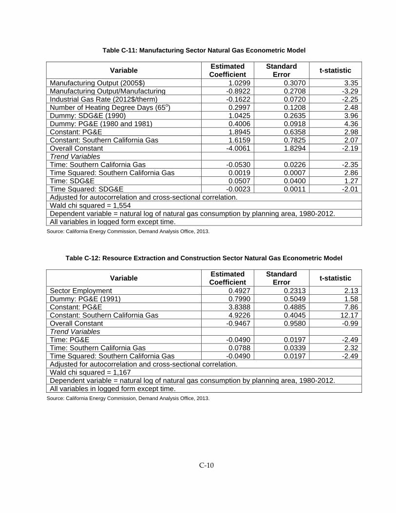
C‐10

Table C-11: Manufacturing Sector Natural Gas Econometric Model



Manufacturing Output (2005$) 1.0299 0.3070 3.35Manufacturing Output/Manufacturing -0.8922 0.2708 -3.29Industrial Gas Rate (2012$/therm) -0.1622 0.0720 -2.25Number of Heating Degree Days (65o) 0.2997 0.1208 2.48Dummy: SDG&E (1990) 1.0425 0.2635 3.96Dummy: PG&E (1980 and 1981) 0.4006 0.0918 4.36Constant: PG&E 1.8945 0.6358 2.98Constant: Southern California Gas 1.6159 0.7825 2.07Overall Constant -4.0061 1.8294 -2.19Trend Variables Time: Southern California Gas -0.0530 0.0226 -2.35Time Squared: Southern California Gas 0.0019 0.0007 2.86Time: SDG&E 0.0507 0.0400 1.27Time Squared: SDG&E -0.0023 0.0011 -2.01Adjusted for autocorrelation and cross-sectional correlation.Wald chi squared = 1,554 Dependent variable = natural log of natural gas consumption by planning area, 1980-2012.All variables in logged form except time.


Table C-12: Resource Extraction and Construction Sector Natural Gas Econometric Model



Sector Employment 0.4927 0.2313 2.13Dummy: PG&E (1991) 0.7990 0.5049 1.58Constant: PG&E 3.8388 0.4885 7.86Constant: Southern California Gas 4.9226 0.4045 12.17Overall Constant -0.9467 0.9580 -0.99Trend Variables Time: PG&E -0.0490 0.0197 -2.49Time: Southern California Gas 0.0788 0.0339 2.32Time Squared: Southern California Gas -0.0490 0.0197 -2.49Adjusted for autocorrelation and cross-sectional correlation.Wald chi squared = 1,167 Dependent variable = natural log of natural gas consumption by planning area, 1980-2012.All variables in logged form except time.


C‐11

Table C-13: Agriculture and Water Pumping Sector Natural Gas Econometric Model



Sector Employment 0.8910 0.0510 17.48Per Capita Income (2012$) 1.1383 0.5302 2.15Commercial Gas Rate (2012$ per mmBTU) -0.0732 0.0937 -0.78Dummy: 2001 -0.1346 0.0903 -1.49Overall Constant -12.0340 5.2987 -2.27Trend Variables Time: PG&E -0.0290 0.0095 -3.06Time: Southern California Gas 0.0249 0.0083 2.99Time: SDG&E -0.0321 0.0120 -2.68Adjusted for autocorrelation and cross-sectional correlation.Wald chi squared = 1,569 Dependent variable = natural log of natural gas consumption by planning area, 1980-2012.All variables in logged form except time.


CED 2014-2024 Revised Forecast Volume 1 - California ... ENERGY DEMAND 2014–2024 REVISED FORECAST...

Documents

Transcript of CED 2014-2024 Revised Forecast Volume 1 - California ... ENERGY DEMAND 2014–2024 REVISED FORECAST...