
C:/Documents and Settings/khoa/Desktop/Kevin's Thesis ...chintha/pdf/thesis/msc_kevin.pdf · In...
105
Abstract R ESEARCH IN WIRELESS COMMUNICATIONS AND NETWORKING has been popularly advocated. It is well-known that a crucial, and thus intensively-studied, issue for improving the performance of wireless networks, i.e., increasing network capacity and operation efficiency, is the efficient management of the available radio resources. This thesis, which consists of three major parts, explores resource allocation problems in wireless data networks using convex optimization. In the first part, a beamforming technique is developed to solve the spectrum sharing problem in wireless networks where secondary users can co-exist with primary users without causing excessive interference. The proposed problems can be solved efficiently using semidefinite programming. The second part investigates different power allocation schemes for multi-user relay networks using ge- ometric programming. Since it is typically not possible to guarantee the quality-of-service for all users in power-limited relay networks, admission control may be necessary. For such cases, an efficient heuristic-based algorithm for solving the joint admission control and power allocation problem is developed. The last part presents a joint cross-layer optimiza- tion approach in multi-hop wireless networks. Given the constraints of the total available energy, network lifetime, and user rates, the problem formulation aims at maximizing the network utility. Although the resulting optimization problem is nonlinear and nonconvex, a convex-based algorithm via two-step optimization is proposed. Furthermore, the problem of maximizing network utility within achievable network lifetime is shown to be quasi-convex. In summary, this thesis research has proposed and then solved several resource allocation problems in wireless networks using convex optimization.
Transcript of C:/Documents and Settings/khoa/Desktop/Kevin's Thesis ...chintha/pdf/thesis/msc_kevin.pdf · In...
Abstract
RESEARCH IN WIRELESS COMMUNICATIONS AND NETWORKING has been
popularly advocated. It is well-known that a crucial, and thus intensively-studied,
issue for improving the performance of wireless networks, i.e., increasing network capacity
and operation efficiency, is the efficient management of the available radio resources.
This thesis, which consists of three major parts, explores resource allocation problems
in wireless data networks using convex optimization. In the first part, a beamforming
technique is developed to solve the spectrum sharing problem in wireless networks where
secondary users can co-exist with primary users without causing excessive interference. The
proposed problems can be solved efficiently using semidefinite programming. The second
part investigates different power allocation schemes for multi-user relay networks using ge-
ometric programming. Since it is typically not possible to guarantee the quality-of-service
for all users in power-limited relay networks, admission control may be necessary. For
such cases, an efficient heuristic-based algorithm for solving the joint admission control and
power allocation problem is developed. The last part presents a joint cross-layer optimiza-
tion approach in multi-hop wireless networks. Given the constraints of the total available
energy, network lifetime, and user rates, the problem formulation aims at maximizing the
network utility. Although the resulting optimization problem is nonlinear and nonconvex, a
convex-based algorithm via two-step optimization is proposed. Furthermore, the problem of
maximizing network utility within achievable network lifetime is shown to be quasi-convex.
In summary, this thesis research has proposed and then solved several resource allocation
problems in wireless networks using convex optimization.
Acknowledgements
Numerous people have supported me during my graduate study at Alberta. A few lines
cannot sufficiently express all my appreciation. Moreover, while I may accidentally miss
out some people whose help deserves to be mentioned, be certain I am most thankful for
your help.
First, I would like to thank my supervisors, Professor Chintha Tellambura and Professor
Sergiy A.Vorobyov for their many suggestions, constant support and inspiration during this
research. I feel providential to have learned from their remarkable combination of technical
knowledge and research enthusiasm. Furthermore, Chintha and Sergiy have taught me
many aspects of carrying out research in the field of wireless communications. My greatest
appreciation is for Sergiy who is also my ‘friend’ for his dedication and professionalism. I
couldn’t find better supervisors at this stage in my research career and I look forward to
our future collaborations. I would also like to thank the committee members, Dr. Ardakani
and Dr. Elmallah for their time and many efforts reading and evaluating my thesis.
I have the fortune to have discussed, interacted and conducted collaborative work with
many distinguished researchers. I have learned immensely from our joint works, from devel-
oping technical skills to presenting nicely the manuscripts. I thank Professor Tho Le-Ngoc
from McGill University, Professor Nicholas D. Sidiropoulos from Technical University of
Crete, Greece, Professor Hai Jiang from University of Alberta, and Professor Ha Nguyen
from University of Saskatchewan for fruitful research collaboration and discussions. Partic-
ularly, I’m grateful to Tho from whom I have learned so much, not only from his insightful
research ideas and suggestions but also from his demonstrated integrity and enthusiasm. I
also thank Professor Hoai An Le-Thi from Paul Verlaine University, France for encouraging
and helping me to study and apply her pioneer mathematical results in wireless communi-

cations and I look forward to our productive collaborative research. Many thanks to Dr.
Long Le from University of Waterloo for his numerous timely advices and support since the
first day we met in HongKong.
Much respect to my friends at the iCORE Wireless Communications Lab. It has been
a truly joy to work and discuss with so many wonderful people at iCORE. While the time
at Edmonton is probably not the best nor even good, I believe that if without you guys, it
could have been much worse. I hope we will keep in touch in the future no matter where
we are. I will miss all of you a lot after an unforgettable period at UofA.
My most compassionate and kindhearted thanks go to my loving wife and daughter,
Hue Chi and Tam Anh. To our Little Princess Tam Anh, I was not there when you were
born; I was not there when you have been growing up. That I couldn’t witness your early
development makes me an unfortunate father. I promise boarding with you and taking you
under my wing for the next trip (and all trips) because you are my everything. To my wife
Chi, I was not there during one of the most difficult time in your life and there’s nothing
more strenuous than being a single-like mom. I’m deeply sorry for not being able to help
our small family. However, your love, understanding and encouragement are never limited,
especially when they are most needed. I enjoy every moment that we talk and plan our
future. Not this thesis but the one we are writing together will be the most significant work
in my life. LET’S UNITE OUR FAMILY!
Finally, I would like to thank my parents who have always been the most important
part of my life, and who have believed in me and supported me throughout. Moreover, our
small family and I in particular are in debt to my mother-in-law for her tremendous love
and care for our Little Princess. Without her help, this thesis couldn’t be completed.
Tran Khoa Phan
Edmonton, May 2008.
Contents
1 Introduction 1
1.1 Motivation . . . . . . . . . . . . . . . . . . . . . . . . . . . . . . . . . . . . 1
1.2 Mathematical Background . . . . . . . . . . . . . . . . . . . . . . . . . . . . 4
1.2.1 Convex problems in standard form . . . . . . . . . . . . . . . . . . . 5
1.2.2 Convex problems in geometric form . . . . . . . . . . . . . . . . . . 6
1.2.3 Lagrange duality theory and KKT optimality conditions . . . . . . . 7
1.2.4 Solving convex problems . . . . . . . . . . . . . . . . . . . . . . . . . 8
1.3 Outline of Thesis . . . . . . . . . . . . . . . . . . . . . . . . . . . . . . . . . 9
2 Spectrum Sharing in Wireless Networks via QoS-Aware Secondary Mul-
ticast Beamforming 11
2.1 Introduction . . . . . . . . . . . . . . . . . . . . . . . . . . . . . . . . . . . . 12
2.2 System Model . . . . . . . . . . . . . . . . . . . . . . . . . . . . . . . . . . . 16
2.3 Beamforming for Secondary Multicasting in Wireless Networks with Perfect
CSI . . . . . . . . . . . . . . . . . . . . . . . . . . . . . . . . . . . . . . . . . 18
2.3.1 Transmit power minimization based beamforming . . . . . . . . . . 18
2.3.2 Interference minimization based beamforming . . . . . . . . . . . . . 19
2.3.3 Maximin fairness based beamforming . . . . . . . . . . . . . . . . . . 21
2.3.4 Worst user SNR-Interference tradeoff analysis . . . . . . . . . . . . . 22
2.4 Solutions . . . . . . . . . . . . . . . . . . . . . . . . . . . . . . . . . . . . . 23
2.4.1 Transmit power minimization based beamforming . . . . . . . . . . 23
2.4.2 Randomization algorithm . . . . . . . . . . . . . . . . . . . . . . . . 24
2.4.3 Interference minimization based beamforming . . . . . . . . . . . . . 26
2.4.4 Maximin fair based beamforming . . . . . . . . . . . . . . . . . . . . 27
2.4.5 Worst user SNR-Interference tradeoff analysis . . . . . . . . . . . . . 28
2.5 SDR via Rank-one Relaxation as the Lagrange Bidual Program . . . . . . . 28
2.6 Beamforming for Secondary Multicasting in Wireless Networks with Channel
Statistics Only . . . . . . . . . . . . . . . . . . . . . . . . . . . . . . . . . . 31
2.7 Simulation Results . . . . . . . . . . . . . . . . . . . . . . . . . . . . . . . . 34
2.7.1 Transmit power minimization based beamforming . . . . . . . . . . 34
2.7.2 Interference minimization based beamforming . . . . . . . . . . . . . 37
2.7.3 Maximin fair based beamforming . . . . . . . . . . . . . . . . . . . . 37
2.7.4 Worst user SNR-Interference tradeoff analysis . . . . . . . . . . . . . 41
2.8 Conclusions . . . . . . . . . . . . . . . . . . . . . . . . . . . . . . . . . . . . 43
3 Power Allocation in Wireless Multi-user Relay Networks 44
3.1 Introduction . . . . . . . . . . . . . . . . . . . . . . . . . . . . . . . . . . . . 45
3.1.1 Literature review . . . . . . . . . . . . . . . . . . . . . . . . . . . . . 45
3.1.2 Motivation and contributions . . . . . . . . . . . . . . . . . . . . . . 46
3.2 System Model . . . . . . . . . . . . . . . . . . . . . . . . . . . . . . . . . . . 48
3.3 Problem Formulations . . . . . . . . . . . . . . . . . . . . . . . . . . . . . . 50
3.3.1 Maximin SNR based power allocation . . . . . . . . . . . . . . . . . 50
3.3.2 Transmit power minimization based power allocation . . . . . . . . . 52
3.3.3 Network throughput maximization based power allocation . . . . . . 53
3.4 Power Allocation in Relay Networks via GP . . . . . . . . . . . . . . . . . . 56
3.4.1 Maximin SNR based power allocation . . . . . . . . . . . . . . . . . 56
3.4.2 Transmit power minimization based power allocation . . . . . . . . . 56
3.4.3 Network throughput maximization based power allocation . . . . . . 56
3.5 Joint Admission Control and Power Allocation . . . . . . . . . . . . . . . . 57
3.5.1 A revised transmit power minimization based power allocation . . . 57
3.5.2 A mathematical framework for joint admission control and power al-
location problem . . . . . . . . . . . . . . . . . . . . . . . . . . . . . 58
3.6 Proposed Algorithm . . . . . . . . . . . . . . . . . . . . . . . . . . . . . . . 59
3.6.1 A reformulation of joint admission control and power allocation problem 59
5
3.6.2 Proposed algorithm . . . . . . . . . . . . . . . . . . . . . . . . . . . 61
3.7 Simulation Results . . . . . . . . . . . . . . . . . . . . . . . . . . . . . . . . 62
3.7.1 Power allocation without admission control . . . . . . . . . . . . . . 62
3.7.2 Joint admission control and power allocation . . . . . . . . . . . . . 67
3.8 Conclusions . . . . . . . . . . . . . . . . . . . . . . . . . . . . . . . . . . . . 71
4 Joint Medium Access Control, Routing and Energy Distribution in Multi-
Hop Wireless Networks 72
4.1 Introduction . . . . . . . . . . . . . . . . . . . . . . . . . . . . . . . . . . . . 73
4.2 Network Model . . . . . . . . . . . . . . . . . . . . . . . . . . . . . . . . . . 73
4.2.1 Link contention graph and maximal cliques . . . . . . . . . . . . . . 75
4.3 Joint Design of MAC, Routing, and Energy Distribution . . . . . . . . . . . 76
4.3.1 Problem formulation . . . . . . . . . . . . . . . . . . . . . . . . . . . 76
4.3.2 Optimal solution . . . . . . . . . . . . . . . . . . . . . . . . . . . . . 77
4.4 Numerical Results . . . . . . . . . . . . . . . . . . . . . . . . . . . . . . . . 81
4.5 Further Discussions . . . . . . . . . . . . . . . . . . . . . . . . . . . . . . . . 84
4.6 Conclusions . . . . . . . . . . . . . . . . . . . . . . . . . . . . . . . . . . . . 85
5 Conclusions and Future Work 86
5.1 Conclusions . . . . . . . . . . . . . . . . . . . . . . . . . . . . . . . . . . . . 86
5.2 Future Work . . . . . . . . . . . . . . . . . . . . . . . . . . . . . . . . . . . 87
References 90
6
List of Tables
3.1 Admission Control: P = 50, PmaxRj
= 50, Running time in seconds . . . . . . 68
3.2 Admission Control: P = 50, PmaxRj
= 20 . . . . . . . . . . . . . . . . . . . . 70
3.3 Admission Control: P = 20, PmaxRj
= 50 . . . . . . . . . . . . . . . . . . . . 70
4.1 Assigned energy and source rate at each node when Tmin = 5000, rLBs = 0.2
and Etot = 100K . . . . . . . . . . . . . . . . . . . . . . . . . . . . . . . . . 83
List of Figures
2.1 A secondary cell with N users and a single primary link . . . . . . . . . . . 17
2.2 Transmit power minimization based beamforming: transmit power versus
users’ SNR thresholds. . . . . . . . . . . . . . . . . . . . . . . . . . . . . . . 35
2.3 Transmit power minimization based beamforming: transmit power versus
interference thresholds. . . . . . . . . . . . . . . . . . . . . . . . . . . . . . . 36
2.4 Interference minimization based beamforming: interference versus user SNR
thresholds. . . . . . . . . . . . . . . . . . . . . . . . . . . . . . . . . . . . . . 38
2.5 Maximin fair based beamforming: worst user SNR versus interference thresh-
olds. . . . . . . . . . . . . . . . . . . . . . . . . . . . . . . . . . . . . . . . . 39
2.6 Maximin fair based beamforming: worst user SNR versus transmit power
with no interference. . . . . . . . . . . . . . . . . . . . . . . . . . . . . . . . 40
2.7 Multi-objective beamforming: worst-user SNR and interference versus trans-
mit power. . . . . . . . . . . . . . . . . . . . . . . . . . . . . . . . . . . . . . 41
2.8 Multi-objective beamforming with different weight parameters: interference
versus worst-user SNR. . . . . . . . . . . . . . . . . . . . . . . . . . . . . . . 42
3.1 Some SNRs versus PRSi, fixed and equal source power PSi
. . . . . . . . . . 55
3.2 A wireless relay system . . . . . . . . . . . . . . . . . . . . . . . . . . . . . . 63
3.3 Data rate versus PmaxRj
, P = 50 . . . . . . . . . . . . . . . . . . . . . . . . . 64
3.4 Data rate versus P , PmaxRj
= 50 . . . . . . . . . . . . . . . . . . . . . . . . . 65
3.5 Transmit power versus γmini and Pmax
Rj. . . . . . . . . . . . . . . . . . . . . 66
3.6 Network throughput versus PmaxRj
, P = 50 . . . . . . . . . . . . . . . . . . . 67
4.1 An example of the network model . . . . . . . . . . . . . . . . . . . . . . . . 79

4.2 Throughput versus minimum network lifetime requirement Tmin. . . . . . . 80
4.3 Throughput versus total available energy Etot . . . . . . . . . . . . . . . . . 82
4.4 Network throughput versus network lifetime requirement Tmin, Etot = 100 KJ 83
9
Chapter 1
Introduction
THE RECENT AND ANTICIPATED DEVELOPMENT of wireless communication
systems has attracted research efforts in investigating methods to increase system
capacity and operation efficiency. The future wireless networks will likely be required to
support services possibly requiring high data rates and provide quality of service (QoS)
for subscribers. The focus of this thesis is on the resource allocation issues in wireless
data networks. Broadly speaking, resource allocation in wireless networks involves efficient
management and distribution of radio resources to participating entities to achieve some
specific goals. Appropriate resource allocation in wireless networks helps to improve the
network capacity and operation efficiency.
1.1 Motivation
Wireless networks have recently emerged as essential means of communications to provide
reliable data communications among many users. The future wireless networks, i.e., cellular,
mesh, or ad hoc networks will likely to be required to provide stringent QoS for users.
This is a challenging task to accomplish, especially for emerging high data rates wireless
applications. Therefore, there is a strong motivation to increase the network capacity and
also stabilize the network operation. Moreover, it is recognized that the issue of efficient
management of communications resources is essential to achieve the aforementioned targets
under difficult circumstances, for instance unreliable propagation channels, interference,
1
user mobility, and resource scarcity. As a result, research on the development of effective
resource allocation techniques in wireless communications has been conducted actively. For
example, power control techniques for conventional cellular communication systems have
been a focus of intensive studies, see [1], [2], [3] and references therein. Since power control
is used to manage interference, it also affects individual user QoS. Resource allocation in
general multi-hop wireless networks includes power allocation, link scheduling, rate control
and so on [4], [5]. Generally, the objectives of resource allocation techniques are to enhance
both communication capacity and lifetime of studied networks, making the most of scarce
radio resources. Efficient and intelligent management of available radio resources is clearly
one of the most, if not the most, challenging task in designing wireless networks.
The radio spectrum available for wireless services is scarce. Therefore, a prime issue in
current wireless systems is the conflict between the increasing demand for wireless services
and the scarce spectrum. Moreover, note that almost all usable bandwidth resource is al-
ready licensed. However, extensive measurements obtained by the FCC [6] indicate that
specific bands of licensed spectrum remain unused for large amounts of time, space, and
frequency due to non-uniform spectral occupation. On the other hand, the implementation
of a variety of wireless devices and emergent wireless services has significantly increased
the spectrum demand. The inconsistency in spectrum licensing and utilization has inspired
much research attention in search for better spectrum access strategies which help to im-
prove system efficiency. As a result, one of the approaches allowing for improved bandwidth
efficiency is the introduction of secondary spectrum licensing, where non-licensed users may
obtain provisional usage of the spectrum. Naturally, secondary spectrum usage happens to
be possible given that the primary users suffer only an acceptable amount of performance
deprivation [7]. Therefore, channel sensing and medium access control (MAC) schemes are
critical for secondary users to detect and access the spectrum opportunity when no primary
users are currently occupying or transmitting. This thesis investigates the spectrum sharing
problem from spectrum underlay perspective [7]. In this context, the secondary access does
not affect the primary users’ operation if the interference power remains below a certain
threshold. Instead of relying on channel sensing and MAC schemes, the benefits of using
multiple antennas i.e., transmit diversity are exploited. Through the use of beamforming
and power control techniques, the interference to the primary network can be effectively
2
controlled. Therefore, even when the primary users are operating, the network of secondary
users is able to exchange information continuously.
Recently, it has been shown that the operation efficiency and QoS of cellular and/or
ad-hoc networks can be increased through the use of relay(s) [8], [9]. In such systems, the
information from the source to the corresponding destination is transmitted via a direct-
link and also forwarded via relays. Due to its significant advantages, for example coverage
extension and performance improvement, relay-assisted communications can be seen as a
candidate for the deployment of future generation networks. Furthermore, in relay net-
works, appropriate power allocation among the participating nodes helps to ensure the
performance and stability of the system. As a result, there have been numerous works
which attempt to optimize the available radio resources, i.e., power and bandwidth to im-
prove the system performance. It is worth mentioning that a single source-destination pair
is typically considered. Indeed, each relay is usually delegated to assist more than one users,
especially when the number of relays is (much) smaller than the number of users. Resource
allocation in a multi-user system usually has to take into account the fairness issue among
users, their relative QoS requirements, channel quality and available resources. Mathemat-
ically, optimizing relay networks with multiple users is very difficult, if tractable, especially
for systems with a large number of sources and relays. Moreover, the power resource is
typically limited and it may happen to be not possible to satisfy QoS requirements for all
users with limited power. Therefore, admission control with some pre-specified objective(s)
should be carried out. Essentially, users are not automatically admitted into the system.
So far, none of the existing works have considered this practical scenario in the context of
relay communications. Therefore, an efficient joint admission control and power allocation
algorithm is desirable.
In the works mentioned above, wireless networks which employ single hop or 2-hop
transmission are considered. However, due to the random deployment and mobility of
wireless nodes, direct i.e., single-hop transmission from the traffic source nodes to the traffic
destination nodes may be impossible. Therefore, multi-hop transmission is necessary where
nodes can forward other nodes’ information, allowing beyond line of sight communication
for wireless nodes. Uninterrupted communications among many users is performed via a
shared wireless channel together with some packet switching protocols. In this case, the
3
efficient design of multi-hop wireless networks is a challenging task.
Recently, the concept of cross-layer design in wireless networks has been investigated
extensively. This is due to the interactions between power allocation, link scheduling,
routing, and rate control in a multi-hop network. Therefore, a cross-layer design across all
layers is important (see, e.g., [10] for an overview). Such a design methodology is shown to
outperform the method of designing each layer separately. Moreover, the existing routing
algorithms adopted in wireless networks try to minimize the total energy consumption which
may cause some particular nodes to run out of energy quickly, especially when nodes are
equipped with equal energy. On the other hand, it has been shown that energy distribution
is critical in multi-hop networks, e.g., sensor and ad hoc networks [11]. Generally, equal
energy assignment to each node may not be optimal. For example, in a mobile ad hoc
network with a wireless gateway, nodes closer to the gateway will likely have more traffic
load, and thus will need more energy. This thesis presents the joint design of medium access
control, routing and energy distribution in a multi-hop wireless network to maximize the
network utility. Each node (or user) has a minimum data rate which must be guaranteed,
as well, the network is able to operate for a given minimum lifetime.
The main mathematical tool for the above resource allocation problems is based on
convex optimization techniques which are briefly described in the next section.
1.2 Mathematical Background
Design and optimization of wireless networks rely heavily on mathematical modeling tools.
Although nonconvex optimization has been shown to be suitable in many scenarios, convex
optimization methods have been used extensively in modeling, analyzing, and designing
of communication systems, for example see [15], [16], [17] and references therein. In par-
ticular, the popularity of convex optimization is also due to the fact that many problems
in communications and signal processing can be naturally formulated or recast as convex
optimization problems. Theoretically, convex optimization is appealing since a local opti-
mum is also a global optimum for a convex problem. Therefore, the computation required
to find the global optimum is much less as compared to the problems with multiple local
optimums. Convex optimization is also attractive because it usually reveals insights into the
4
structure of the optimal solution and the design itself. The last feature usually can not be
obtained from nonconvex optimization methods since they concentrate on the computation
of optimum points. Furthermore, the availability of software, for example [12] and [13], for
solving convex problems makes convex optimization even more popular.
Suppose that S is a subset of Rn for n ≥ 1. A function f : Rn −→ R on a convex set
S1 is a convex function if for any two points x,y ∈ S
f(ζx + (1 − ζ)y) ≤ ζf(x) + (1 − ζ)f(y), 0 ≤ ζ ≤ 1
In other words, along any line segment in S, f is less than or equal to the value of the linear
function agreeing with f at the end points. One says f is concave if −f is convex. Convex
functions are closed under summation, positive scaling, and pointwise maximum operation.
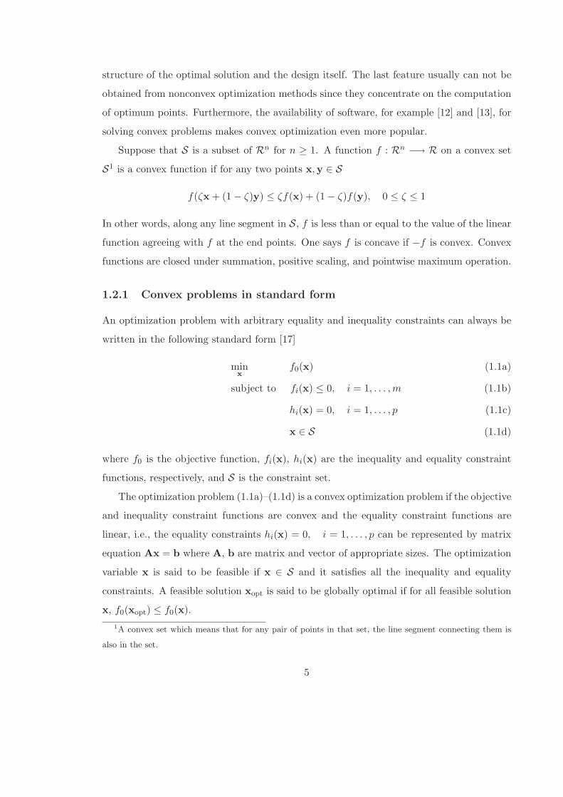
1.2.1 Convex problems in standard form
An optimization problem with arbitrary equality and inequality constraints can always be
written in the following standard form [17]
minx
f0(x) (1.1a)
subject to fi(x) ≤ 0, i = 1, . . . , m (1.1b)
hi(x) = 0, i = 1, . . . , p (1.1c)
x ∈ S (1.1d)
where f0 is the objective function, fi(x), hi(x) are the inequality and equality constraint
functions, respectively, and S is the constraint set.
The optimization problem (1.1a)–(1.1d) is a convex optimization problem if the objective
and inequality constraint functions are convex and the equality constraint functions are
linear, i.e., the equality constraints hi(x) = 0, i = 1, . . . , p can be represented by matrix
equation Ax = b where A, b are matrix and vector of appropriate sizes. The optimization
variable x is said to be feasible if x ∈ S and it satisfies all the inequality and equality
constraints. A feasible solution xopt is said to be globally optimal if for all feasible solution
x, f0(xopt) ≤ f0(x).
1A convex set which means that for any pair of points in that set, the line segment connecting them is
also in the set.
5
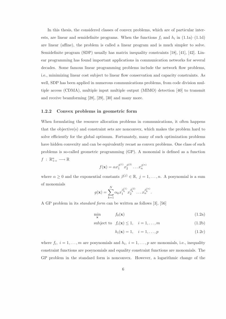
In this thesis, the considered classes of convex problems, which are of particular inter-
ests, are linear and semidefinite programs. When the functions fi and hi in (1.1a)–(1.1d)
are linear (affine), the problem is called a linear program and is much simpler to solve.
Semidefinite program (SDP) usually has matrix inequality constraints [18], [41], [42]. Lin-
ear programming has found important applications in communication networks for several
decades. Some famous linear programming problems include the network flow problems,
i.e., minimizing linear cost subject to linear flow conservation and capacity constraints. As
well, SDP has been applied in numerous communications problems, from code division mul-
tiple access (CDMA), multiple input multiple output (MIMO) detection [40] to transmit
and receive beamforming [28], [29], [30] and many more.
1.2.2 Convex problems in geometric form
When formulating the resource allocation problems in communications, it often happens
that the objective(s) and constraint sets are nonconvex, which makes the problem hard to
solve efficiently for the global optimum. Fortunately, many of such optimization problems
have hidden convexity and can be equivalently recast as convex problems. One class of such
problems is so-called geometric programming (GP). A monomial is defined as a function
f : Rn++ −→ R
f(x) = αxβ(1)
1 xβ(2)
2 . . . xβ(n)
n
where α ≥ 0 and the exponential constants β(j) ∈ R, j = 1, . . . , n. A posynomial is a sum
of monomials
g(x) =
N∑
k=1
αkxβ
(1)k
1 xβ
(2)k
2 . . . xβ
(n)k
n .
A GP problem in its standard form can be written as follows [3], [56]
minx
f0(x) (1.2a)
subject to fi(x) ≤ 1, i = 1, . . . , m (1.2b)
hi(x) = 1, i = 1, . . . , p (1.2c)
where fi, i = 1, . . . , m are posynomials and hi, i = 1, . . . , p are monomials, i.e., inequality
constraint functions are posynomials and equality constraint functions are monomials. The
GP problem in the standard form is nonconvex. However, a logarithmic change of the
6
variables, multiplicative constants, and the function values builds an equivalent convex
problem in new variables. The background and applications of GP in communications can
be found in [3], [17], [56]. In summary, GP is a nonlinear, nonconvex optimization problem
that can be recast as a nonlinear, convex problem. The problems of power allocation in
multi-user wireless relay networks in Chapter 3 are cast as GP problems.
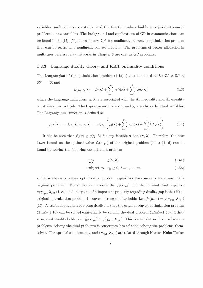
1.2.3 Lagrange duality theory and KKT optimality conditions
The Langrangian of the optimization problem (1.1a)–(1.1d) is defined as L : Rn × Rm ×Rp −→ R and
L(x, γ, λ) = f0(x) +m∑
i=1
γifi(x) +
p∑
i=1
λihi(x) (1.3)
where the Lagrange multipliers γi, λi are associated with the ith inequality and ith equality
constraints, respectively. The Lagrange multipliers γi and λi are also called dual variables.
The Lagrange dual function is defined as
g(γ, λ) = infx∈SL(x, γ, λ) = infx∈S
(
f0(x) +
m∑
i=1
γifi(x) +
p∑
i=1
λihi(x)
)
. (1.4)
It can be seen that f0(x) ≥ g(γ, λ) for any feasible x and (γ, λ). Therefore, the best
lower bound on the optimal value f0(xopt) of the original problem (1.1a)–(1.1d) can be
found by solving the following optimization problem
maxγ,λ
g(γ, λ) (1.5a)
subject to γi ≥ 0, i = 1, . . . , m (1.5b)
which is always a convex optimization problem regardless the convexity structure of the
original problem. The difference between the f0(xopt) and the optimal dual objective
g(γopt, λopt) is called duality gap. An important property regarding duality gap is that if the
original optimization problem is convex, strong duality holds, i.e., f0(xopt) = g(γopt, λopt)
[17]. A useful application of strong duality is that the original convex optimization problem
(1.1a)–(1.1d) can be solved equivalently by solving the dual problem (1.5a)–(1.5b). Other-
wise, weak duality holds, i.e., f0(xopt) > g(γopt, λopt). This is a helpful result since for some
problems, solving the dual problems is sometimes ’easier’ than solving the problems them-
selves. The optimal solutions xopt and (γopt, λopt) are related through Karush-Kuhn-Tucker
7
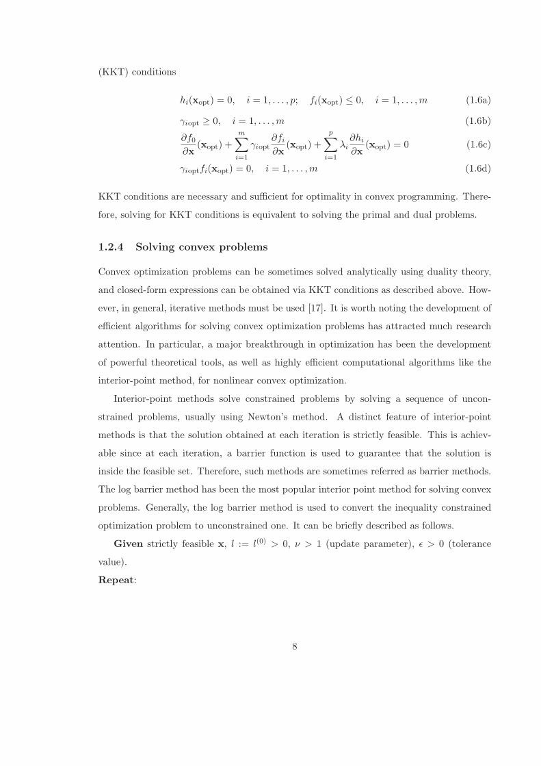
(KKT) conditions
hi(xopt) = 0, i = 1, . . . , p; fi(xopt) ≤ 0, i = 1, . . . , m (1.6a)
γiopt ≥ 0, i = 1, . . . , m (1.6b)
∂f0
∂x(xopt) +
m∑
i=1
γiopt∂fi
∂x(xopt) +
p∑
i=1
λi∂hi
∂x(xopt) = 0 (1.6c)
γioptfi(xopt) = 0, i = 1, . . . , m (1.6d)
KKT conditions are necessary and sufficient for optimality in convex programming. There-
fore, solving for KKT conditions is equivalent to solving the primal and dual problems.
1.2.4 Solving convex problems
Convex optimization problems can be sometimes solved analytically using duality theory,
and closed-form expressions can be obtained via KKT conditions as described above. How-
ever, in general, iterative methods must be used [17]. It is worth noting the development of
efficient algorithms for solving convex optimization problems has attracted much research
attention. In particular, a major breakthrough in optimization has been the development
of powerful theoretical tools, as well as highly efficient computational algorithms like the
interior-point method, for nonlinear convex optimization.
Interior-point methods solve constrained problems by solving a sequence of uncon-
strained problems, usually using Newton’s method. A distinct feature of interior-point
methods is that the solution obtained at each iteration is strictly feasible. This is achiev-
able since at each iteration, a barrier function is used to guarantee that the solution is
inside the feasible set. Therefore, such methods are sometimes referred as barrier methods.
The log barrier method has been the most popular interior point method for solving convex
problems. Generally, the log barrier method is used to convert the inequality constrained
optimization problem to unconstrained one. It can be briefly described as follows.
Given strictly feasible x, l := l(0) > 0, ν > 1 (update parameter), ǫ > 0 (tolerance
value).
Repeat:
8
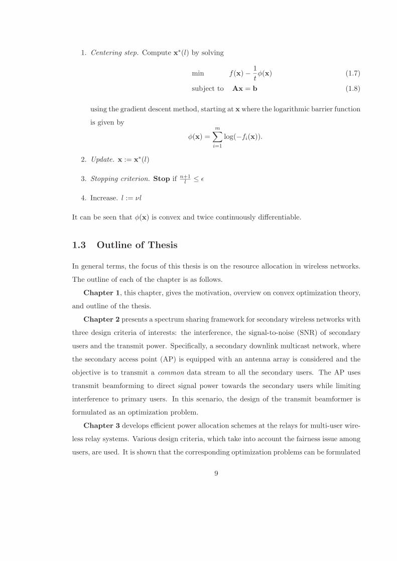
1. Centering step. Compute x∗(l) by solving
min f(x) − 1
tφ(x) (1.7)
subject to Ax = b (1.8)
using the gradient descent method, starting at x where the logarithmic barrier function
is given by
φ(x) =m∑
i=1
log(−fi(x)).
2. Update. x := x∗(l)
3. Stopping criterion. Stop if n+1l ≤ ǫ
4. Increase. l := νl
It can be seen that φ(x) is convex and twice continuously differentiable.
1.3 Outline of Thesis
In general terms, the focus of this thesis is on the resource allocation in wireless networks.
The outline of each of the chapter is as follows.
Chapter 1, this chapter, gives the motivation, overview on convex optimization theory,
and outline of the thesis.
Chapter 2 presents a spectrum sharing framework for secondary wireless networks with
three design criteria of interests: the interference, the signal-to-noise (SNR) of secondary
users and the transmit power. Specifically, a secondary downlink multicast network, where
the secondary access point (AP) is equipped with an antenna array is considered and the
objective is to transmit a common data stream to all the secondary users. The AP uses
transmit beamforming to direct signal power towards the secondary users while limiting
interference to primary users. In this scenario, the design of the transmit beamformer is
formulated as an optimization problem.
Chapter 3 develops efficient power allocation schemes at the relays for multi-user wire-
less relay systems. Various design criteria, which take into account the fairness issue among
users, are used. It is shown that the corresponding optimization problems can be formulated
9

as GP problems. Therefore, optimal power allocation can be obtained efficiently even for
large-scale networks using convex optimization techniques. Another issue is that it may be
impossible to satisfy QoS requirements for all users with limited power. In such scenarios,
some sort of admission control with pre-specified objective(s) should be carried out. In
this chapter, an efficient joint admission control and power allocation algorithm is devel-
oped which aims at maximizing the number of users that can be admitted and served with
(possibly different) QoS demands.
Chapter 4 presents the joint design of MAC, routing and energy distribution in a multi-
hop wireless network, where the QoS of each node must be guaranteed in the minimum
required network lifetime, and the network utility within this lifetime is to be maximized.
The wireless relay service provisioning is formulated as a nonconvex network utility max-
imization (NUM) problem. It is proved that the aforementioned problem is equivalent to
a two-step convex problem. It is also proved that the NUM problem that maximizes the
network utility within achievable network lifetime is a quasi-convex problem, and thus can
be efficiently solved by traditional methods.
Chapter 5 concludes the thesis summarizing the obtained results and proposing some
possible future work.
10
Chapter 2
Spectrum Sharing in Wireless
Networks via QoS-Aware
Secondary Multicast Beamforming
SECONDARY SPECTRUM USAGE HAS THE POTENTIAL to considerably increase
spectrum utilization. In this chapter, quality-of-service (QoS)-aware spectrum under-
lay of a secondary multicast network is considered. A multi-antenna secondary access point
(AP) is used for multicast (common information) transmission to a number of secondary
single-antenna receivers. The idea is that beamforming can be used to steer power towards
the secondary receivers while limiting sidelobes that cause interference to primary receivers.
Various optimal beamformer design formulations are proposed, motivated by different “co-
habitation” scenarios, including robust design that is applicable with limited channel state
information at the secondary AP. These formulations are NP-hard computational problems;
yet it is shown how convex approximation-based multicast beamforming tools (originally
developed without regard to primary interference constraints) can be adapted to work in
a spectrum underlay context. Extensive simulation results demonstrate the effectiveness
of the proposed approaches and provide insights on the tradeoffs between different design
criteria. The work in this chapter can be seen as an extension to the work of Sidiropoulos et.
al. [29] for conventional cellular system with further investigation on the distinct features
of secondary spectrum usage.
11
The rest of the chapter is organized as follows. Section 2.1 overviews the literature on
cognitive radios and summarizes the contributions. In Section 2.2, the system model and
assumptions are presented. Practical formulations for the multicast downlink beamforming
problem are developed in Section 2.3. Section 2.4 shows how semi-definite relaxation (SDR)
and tailored randomization techniques can be employed to solve the problems proposed in
Section 2.3. Section 2.5 provides insights into the method of SDR for one of the considered
beamforming problems. The extension to the case of probabilistically-constrained beam-
forming with unknown instant channels is given in Section 2.6. Numerical results which
demonstrate the effectiveness of our proposed approach are presented in Section 2.7, which
is followed by the conclusions in Section 2.8.
2.1 Introduction
Recently, there is a rapid growth in spectrum demand especially due to the implementation
of a variety of wireless devices and emergent wireless services. However, almost all us-
able frequencies have already been licensed. At the same time, extensive measurements [6]
indicate that many frequency bands remain unused for as large as 85% of time due to
non-uniform spectral occupation. The low utilization of licensed spectrum has inspired a
significant amount of research in searching for better spectrum access strategies for improved
efficiency. One of the approaches allowing for improved bandwidth efficiency is the intro-
duction of secondary spectrum licensing, where non-licensed users may obtain provisional
usage of the spectrum. Naturally, secondary spectrum usage happens to be possible only if
secondary network causes an acceptable (small) amount of performance degradation to the
primary users [52]. Therefore, a secondary network should take into account the impact of
its operation onto the transmission quality of the co-existing primary users. Therefore, it
poses the key challenge in secondary spectrum usage: how to construct spectrum sharing
schemes such that primary users would be protected from excessive interference caused by
the operation of secondary network, and at the same time, the performance of secondary
users would be guaranteed? Addressing this issue successfully will make secondary spectrum
licensing feasible, and thus, likely to improve the overall network efficiency.
Existing works on spectrum sharing/access so far mainly exploit either temporal or
12
spatial spectrum opportunity. For example, a design framework to maximize the throughput
of a secondary network is proposed in [48] based on partially observable Markov decision
process. This approach combines the design of spectrum sensor at the physical layer with
that of spectrum sensing and access policies at the medium access control (MAC) layer. A
graph-theoretic model for spectrum sharing among secondary users is proposed in [20] where
different objective functions are investigated. According to this approach, secondary users
collaboratively utilize the available spectrum holes for the entire network while avoiding
interference with its neighbors. An ad hoc secondary network configuration where the
secondary users operate over the spectrum resources unoccupied by the primary system is
proposed in [21]. This work is based on the so-called bandwidth sharing approach and the
secondary network does not interact with the primary users. In all aforementioned works, it
is assumed that the secondary users first listen to the environment, then decide to transmit
if some channels are not currently used by primary users. The latter strategy is commonly
called as spectrum overlay [52]. Therefore, the interference to the primary users in the
aforementioned works can only be caused by the sensing errors.
In the literature, there also exist several works which tackle the dynamic spectrum access
problem from an adaptive, game theoretic learning perspective. That is, secondary users
behave as game players which compete for unused radio channels. To this extend, each
player aims at capturing enough radio resources to satisfy its spectral demand. Moreover,
it should be noted that this approach happens to be viable only when channel sensing and
allocation occur much faster than changes in secondary user resource demands. For example,
a class of decentralized algorithms in which the secondary users are able to adapt to each
others’ activities and changes in their operating environment is developed in [23], [24]. The
formulation of distributed channel allocation problem using game theory is proposed in [22].
However, in these works the primary users are not explicitly protected from interference
due to spectrum access of secondary users.
In this thesis, the spectrum sharing problem is investigated from the spectrum underlay
perspective [52]. The concept of ‘interference temperature’ has been introduced in [31],
and it indicates the allowable interference level at the primary receivers. Practically, the
secondary access does not affect primary licensees’ operation only if the interference power
remains below a certain threshold. While most of the current literature on secondary spec-
13
trum access relies on channel sensing and medium access control (MAC) schemes, we exploit
the benefits of using multiple antennas. Through the use of beamforming and power control
techniques, the interference to the primary network can be effectively controlled. There-
fore, even when the primary users are operating, the network of secondary users is able
to exchange information continuously. This alleviates spectrum sensing demands, which
are stringent in overlay systems. Whereas spectrum underlay requires channel estimates,
spectrum overlay requires activity detection at a much faster time scale. Similar to clas-
sical random access protocols such as carrier-sense multiple access, activity detection is
compounded by the hidden terminal problem, which is common in wireless.
In traditional cellular systems, the beamforming and power control techniques are well-
known, and are used to control co-channel interference [27], [28], [29], [30]. In [27], an
iterative algorithm is proposed to jointly compute a set of feasible transmit beamforming
weight vectors and power allocations such that the signal-to-interference-plus-noise ratio
(SINR) at each mobile user would be greater than a target value. The approach developed
in [28], [29], [30] is based on convex optimization via semi-definite programming (SDP). For
the latter approach, solution can be efficiently computed using standard interior-point algo-
rithms with guaranteed convergence speed and complexity [13]. Note that in [27] and [28],
the authors consider the transmission of independent information to each of the downlink
users, while a broadcast scenario is considered in [29]. Moreover, an approach to robust
adaptive beamforming in the presence of an arbitrary unknown signal steering vector (chan-
nel) mismatch based on the optimization of the worst-case performance is developed in [30].
In the context of secondary networks, the transmit power control and dynamic spectrum
management problem has been initiated in [31]. In [32], two iterative algorithms have been
proposed for jointly optimal power control and beamforming. The latter work considers
two different system scenarios of spectrum sharing: with and without cooperation between
the secondary and primary networks. Moreover, the uplink-downlink duality has been used
to convert the downlink beamforming problem into the virtual uplink one [33]. In [34], an
admission control algorithm which is performed jointly with power/rate allocation based on
maximin fairness criterion is proposed.
This chapter presents a spectrum sharing framework for secondary wireless networks
by using three different optimization criteria: the interference minimization, the signal-to-
14
noise ratio (SNR) of secondary users maximization, or the transmit power minimization.
Specifically, a secondary downlink multicast network is considered, where the secondary
access point (AP) is equipped with an antenna array and the objective is to transmit a
common data stream to all the secondary users. The AP uses transmit beamforming to
direct signal power towards secondary users while limiting interference to primary users.
In this scenario, the design of the transmit beamformer is formulated as an optimization
problem. Our work can be also viewed as an extension of the work in [29] for traditional
cellular systems with distinct features of secondary networks. Besides the optimization
viewpoint, our work can also be seen as an investigation of the interactions between the
aforementioned criteria. In fact, the latter purpose is our initial motivation.
The following optimization problems are considered in this work in the context of cog-
nitive radio:
• Minimization of the total transmission power subject to constraints on the QoS for
each receiver;
• Minimization of the interference subject to constraints on the SNR of secondary users
and transmit power;
• Maximization of the smallest receiver SNR over the intended secondary users subject
to constraints on the transmit power and interference level;
• A weighted tradeoff formulation that balances interference caused to the primary
system versus the minimum SNR in the secondary system.
It should be noted that all the above problem formulations require perfect channel knowledge
at the design center. However, such channel knowledge may not be always easily accessible
in practice. Therefore, an extension to the case when the AP can not track the channel to
the secondary users is also provided. In this case, by exploiting the statistical characteristic
of the channel gains, it can be shown that a probabilistic constraint on the SNR of the
secondary users is equivalent to a lower bound constraint on the transmit power. Although
the proposed optimization problems are shown to be nonconvex and NP-hard, a convex
relaxation technique via SDP is adopted. Based on this technique the solutions that are
close to being optimal can be efficiently found [29], [37], [38].
15
2.2 System Model
A network which consists of several secondary users in the presence of multiple primary
transmitter-receiver links is considered. An example of such network can be the temporary
deployment of a secondary wireless local area network (WLAN) in the area of an existing
primary WLAN. The particular scenario considered here is one in which the secondary
WLAN AP transmits common information to all secondary users. The secondary AP (or
base station) is equipped with M antennas while each of N secondary and K primary users
has single antenna. Since the primary and secondary networks coexist, the operation of
the latter must not cause excessive interference to the former. This can be accomplished in
two ways. One is to severely limit the total transmission power of the secondary AP, which
will limit the interference to any primary receiver irrespective of the associated coupling
channel vector direction, by virtue of the Cauchy-Schwartz inequality. Knowing the maximal
coupling channel norm is then sufficient to bound interference power. The drawback of this
approach is that it will typically over-constrain the transmission power and thus the spectral
efficiency of the secondary network. A more appealing alternative for the secondary AP is
to estimate the channel vectors between its antenna array and the primary (and secondary)
receivers and use beamforming techniques. If the primary system operates in a time-division
duplex (TDD) mode, this can be accomplished by monitoring primary transmissions in the
reverse link.1 Otherwise, blind beamforming techniques could be employed. Alternatively,
the primary system could cooperate (under a ‘sublet’ agreement) with the secondary system
to pass along channel estimates (see also [25], [32], [34] and references therein) - albeit this is
far less appealing from a practical standpoint. Although perfect CSI will not be available in
the considered scenario, accurate CSI can be obtained in certain (e.g., fixed wireless or low-
mobility) cases. Either way, (approximate or partial/statistical) knowledge of the primary
channel vectors enables (approximate) spatial nulling to protect the primary receivers while
directing higher power towards the secondary receivers - thereby increasing the transmission
rate for the secondary system.
1In this case, the secondary AP can listen to the transmission from the primary receivers and estimate
the channel vectors from itself to primary receivers, assuming reciprocity. Note that this approach is possible
only if the same frequency is used for duplexing.
16
Cell phone
Cell phone
Cell phone
Comm. Tower
Cell phone
User 1
User 2
Primary transmitter
Primary receiver
User N
Interference
Multiple-antenna
BS
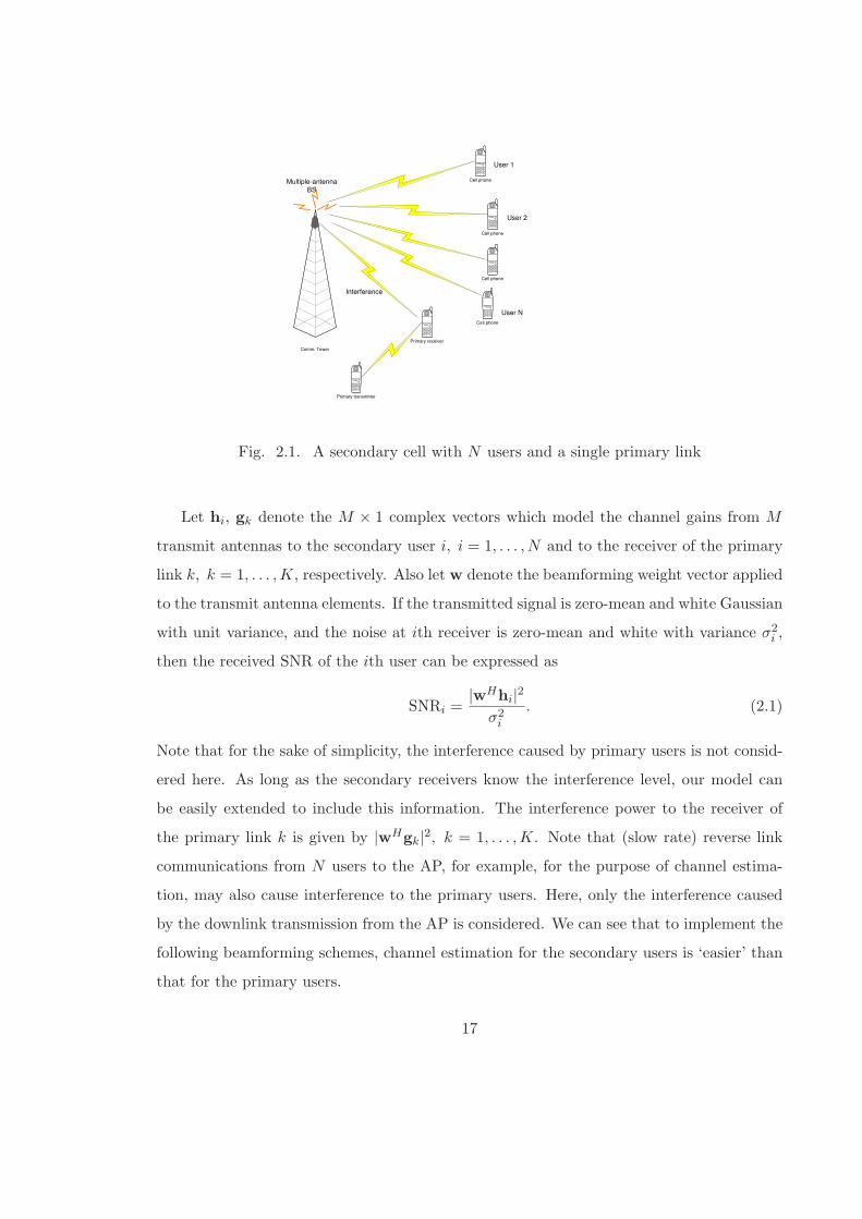
Fig. 2.1. A secondary cell with N users and a single primary link
Let hi, gk denote the M × 1 complex vectors which model the channel gains from M
transmit antennas to the secondary user i, i = 1, . . . , N and to the receiver of the primary
link k, k = 1, . . . , K, respectively. Also let w denote the beamforming weight vector applied
to the transmit antenna elements. If the transmitted signal is zero-mean and white Gaussian
with unit variance, and the noise at ith receiver is zero-mean and white with variance σ2i ,
then the received SNR of the ith user can be expressed as
SNRi =|wHhi|2
σ2i
. (2.1)
Note that for the sake of simplicity, the interference caused by primary users is not consid-
ered here. As long as the secondary receivers know the interference level, our model can
be easily extended to include this information. The interference power to the receiver of
the primary link k is given by |wHgk|2, k = 1, . . . , K. Note that (slow rate) reverse link
communications from N users to the AP, for example, for the purpose of channel estima-
tion, may also cause interference to the primary users. Here, only the interference caused
by the downlink transmission from the AP is considered. We can see that to implement the
following beamforming schemes, channel estimation for the secondary users is ‘easier’ than
that for the primary users.
17
2.3 Beamforming for Secondary Multicasting in Wireless Net-
works with Perfect CSI
2.3.1 Transmit power minimization based beamforming
As discussed above, the operation of the secondary network should not cause excessive
interference to the primary receivers, and simultaneously the performance of secondary
users should be guaranteed. It is well-known that by exploiting the available CSI, one can
efficiently control the QoS of the receivers using optimized transmission. Given lower bound
constraints on the received SNR of each secondary user and upper bound constraints on the
interference to the primary users, the problem of designing the beamformer which minimizes
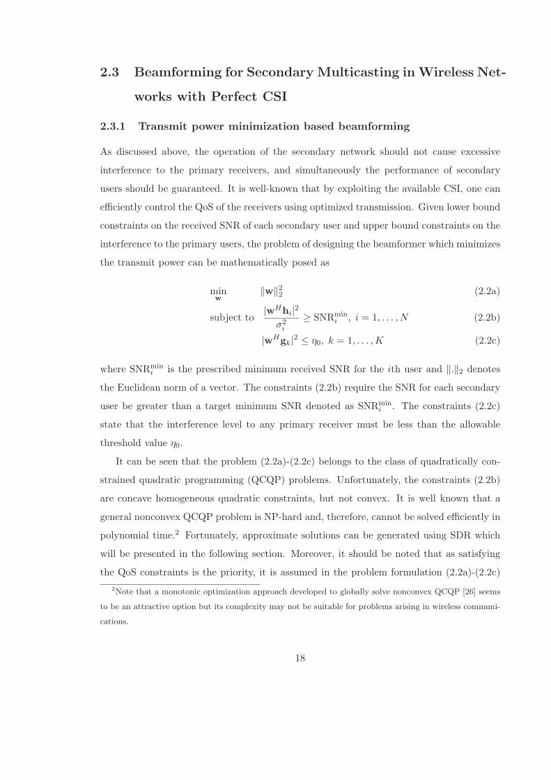
the transmit power can be mathematically posed as
minw
‖w‖22 (2.2a)
subject to|wHhi|2
σ2i
≥ SNRmini , i = 1, . . . , N (2.2b)
|wHgk|2 ≤ η0, k = 1, . . . , K (2.2c)
where SNRmini is the prescribed minimum received SNR for the ith user and ‖.‖2 denotes
the Euclidean norm of a vector. The constraints (2.2b) require the SNR for each secondary
user be greater than a target minimum SNR denoted as SNRmini . The constraints (2.2c)
state that the interference level to any primary receiver must be less than the allowable
threshold value η0.
It can be seen that the problem (2.2a)-(2.2c) belongs to the class of quadratically con-
strained quadratic programming (QCQP) problems. Unfortunately, the constraints (2.2b)
are concave homogeneous quadratic constraints, but not convex. It is well known that a
general nonconvex QCQP problem is NP-hard and, therefore, cannot be solved efficiently in
polynomial time.2 Fortunately, approximate solutions can be generated using SDR which
will be presented in the following section. Moreover, it should be noted that as satisfying
the QoS constraints is the priority, it is assumed in the problem formulation (2.2a)-(2.2c)
2Note that a monotonic optimization approach developed to globally solve nonconvex QCQP [26] seems
to be an attractive option but its complexity may not be suitable for problems arising in wireless communi-
cations.
18
that the AP is endowed with unlimited power. This is because the computed objective
value may turn out to be arbitrarily large.
Observation 1: At optimality, at least one of the constraints (2.2b) must be met with
equality. Otherwise, the beamformer can be scaled down by an appropriate coefficient
such that all the constraints are still met, and at the same time the objective function is
decreased.
It also worth noting that the beamforming problem (2.2a)-(2.2c) is not always feasible.
Geometrically, the feasible region of (2.2a)-(2.2c) is the region determined by the intersection
of the exteriors of N co-centered ellipsoids and of the interiors of K co-centered ellipsoids
[35]. Obviously, this region may turn out to be empty. Moreover, the set of interference
constraints (2.2c) can be satisfied by making the values of the beamformer vector w small.
On the other hand, the set of SNR constraints (2.2b) may require large values of the
beamformer vector w. Therefore, the two types of constraints can ‘conflict’ with each
other. As a result, infeasibility is possible for example when minimum SNR targets SNRmini ,
i = 1, . . . , N are too high or the number of secondary users N is too large. However, one
can argue that by means of Cauchy-Schwartz inequality, the set of interference constraints
(2.2c) can be replaced by an upper bound constraint on the transmit power. However, this
approach admits an overly conservative design, thus, is sub-optimal.
2.3.2 Interference minimization based beamforming
Due to the broadcasting nature of wireless transmission, the operation of the secondary
network inevitably degrades the reception quality of the primary links by creating inter-
ference at the primary receivers. Therefore, a possible problem formulation is to minimize
the interference level while each secondary user has its SNR above some threshold. This
formulation corresponds to the scenarios when the secondary network lease the spectrum
of primary network, thus QoS requirements for secondary users must be guaranteed. In
practice, the QoS requirements are specified by the agreement with the primary network.
19
Then, mathematically, the beamforming problem can be formulated as
minw
K∑
k=1
|wHgk|2 (2.3a)
subject to ‖w‖22 ≤ P (2.3b)
|wHhi|2σ2
i
≥ SNRmini , i = 1, . . . , N. (2.3c)
Similarly to the problem (2.2a)-(2.2c), it can be shown that the problem (2.3a)-(2.3c) is a
nonconvex QCQP due to the constraints (2.3c). Practically, the constraint on the maxi-
mum allowable transmit power is applicable for the power-limited communication systems.
Moreover, the constraint (2.3b) is necessary here because of the following lemma.
LEMMA 2.1: Suppose that K ≤ M , and no hi, ∀i belongs to the orthogonal complement
of the nullspace of the matrix G = [g1,g2, . . . ,gK ]H . When there is no constraint on the
transmit power in (2.3a)-(2.3c), the optimal interference value is zero.
PROOF: Under the conditions of the lemma we can always find a vector w0 as a
solution of the set of equalities |wHgk|2 = 0, ∀k = 1, . . . , K, and w0 is not orthogonal to
any of gk’s. Then, by scaling the length of such vector by an appropriate factor, we can
always satisfy all the received SNR constraints. Therefore, all the constraints are met and
the objective function value is 0. �
Observation 2: Since the objective function (2.3a) is decreasing w.r.t. ‖w‖2, at op-
timality, at least one of the constraints (2.3c) must be met with equality. Otherwise, the
beamformer can be scaled down such that all the constraints are still met, and the objective
function is decreased.
Observation 3: If the elements of hi, ∀i and gk, ∀k are drawn from a distribution, which
is assumed to be continuous with respect to the Lebesgue measure in CM , the condition
that no hi, ∀i belongs to the orthogonal complement of the nullspace of the matrix G =
[g1,g2, . . . ,gK ]H holds almost surely [36].
It can be easily seen that the interference minimization based beamforming problem
(2.3a)-(2.3c) is not always feasible. In fact, the feasibility of the problem (2.3a)-(2.3c)
depends on many factors such as the number of transmit antennas M , the number of
receivers N , the channel realizations hi, i = 1, . . . , N , and the constraints for secondary
users, i.e., the SNR thresholds and the available transmit power. A practical implication
20
of the infeasibility is that it may not be possible to serve all the secondary subscribers at
their desired QoS from a single power-limited AP, and an admission control schemes may
be required. However, investigation of such possibilities is outside of the scope of this work
and is a subject of future research.
Furthermore, since the objective function in the problem (2.3a)-(2.3c) is a sum of in-
terferences to all primary receivers, there may be excessive interferences to some particular
primary receivers at optimality. Therefore, another beamforming problem which prevents
primary users from extreme interferences can be formulated as follows
minw
maxk=1,...,K
{
|wHgk|2}
(2.4a)
subject to The constraints (2.3b)–(2.3c). (2.4b)
For the interference minimization based beamforming, only the optimization problem (2.3a)-
(2.3c) is considered in the sequel.
2.3.3 Maximin fairness based beamforming
The performance of the worst serviced user(s) is often of concern to the cellular network
operator. Therefore, in addition to providing preferential treatment to high priority con-
nections, the services for low priority users must be taken into account. The beamforming
problem which aims at maximizing the minimum received SNR over all receivers subject to
the bound on total transmit power and interference constraint on the primary user can be
written as
maxw
mini=1,...,N
{
|wHhi|2σ2
i
}
(2.5a)
subject to ‖w‖22 ≤ P (2.5b)
|wHgk|2 ≤ η0, k = 1, . . . , K. (2.5c)
Note that other forms of fairness, for example, weighted fairness can be considered. In this
case, the objective function will be a weighted sum of the received SNRs with different
weights for different users. The following lemma is in order.
LEMMA 2.2: At optimality, either one of the constraints in (2.5b) or (2.5c) will be met
with equality.
21
PROOF: It can be proved by contradiction. Suppose that wopt is the optimal solution
and none of the constraints is met with equality. Then, the beamformer wopt can be scaled
by a factor α > 1 which is determined by
α = min
{
P
‖wopt‖22
,η0
|wHoptgk|2k=1,...,K
}
> 1. (2.6)
It can be seen that the resulting beam-vector w = αwopt is also feasible. This will improve
the objective function, thus contradicting the optimality assumption since the objective
function mini=1,...,N
{
|wHhi|
2
σ2i
}
is an increasing function of the norm of w. �
Introducing a new variable t, the problem (2.5a)-(2.5c) can be equivalently rewritten as
the following optimization problem
minw, t
−t (2.7a)
subject to|wHhi|2
σ2i
≥ t, i = 1, . . . , N (2.7b)
‖w‖22 ≤ P, t ≥ 0 (2.7c)
|wHgk|2 ≤ η0, k = 1, . . . , K. (2.7d)
It is easy to check that the constraints (2.7c)-(2.7d) are convex on w and t. However, the
constraints (2.7b) are nonlinear and nonconvex on w and t. Hence, the problem (2.7a)-
(2.7d) also belongs to the class of semi-infinite nonconvex QCQP, and thus, is NP-hard.
Interesting enough, the problem (2.7c)-(2.7d) contains the one in [29] as a special case. Note
that in [29], the constraint on total transmission power had to be met with equality. This
is not the case for our problem (2.7a)-(2.7d) due to the presence of the primary interference
constraints. Therefore, it is not surprising that at least one of the constraints (2.7b) must
be achieved with equality at optimality. Otherwise, t can always be increased, and thus,
the objective function can be decreased.
2.3.4 Worst user SNR-Interference tradeoff analysis
The interference to the primary users is minimized in the problem (2.3a)-(2.3c), while
the minimum received SNR over all receivers is maximized in the problem (2.5a)-(2.5c).
Obviously, simultaneous maximization of the users’ received SNRs and minimization of the
interference caused to the primary users are desirable. However, there is a tradeoff between
22
these two objectives. Given the available transmit power, a mathematical model for tradeoff
analysis between these two objectives can be posed as
maxw
p2 mini=1,...,N
{
|wHhi|2σ2
i
}
− p1 maxk=1,...,K
{
|wHgk|2}
(2.8a)
subject to ‖w‖22 ≤ P. (2.8b)
The optimization problem (2.8a)-(2.8b) can be shown to be a nonconvex QCQP prob-
lem, i.e., convex maximization problem and it is also NP-hard. The arbitrary importance
parameters p1 and p2 quantify the desire to make the largest interference level small and
the SNR of the worst user large, respectively. Moreover, the ratio of p1 and p2, i.e., p1/p2,
can be seen as a relative importance of the interference to the primary users and the per-
formance of the secondary users. In particular, for a fixed value of p2, a larger value of p1
results in smaller interference at the cost of performance degradation for the worst user in
the network. Without loss of generality, we can set p2 = 1 and by varying p1 > 0, obtain
the Pareto optimal points by solving (2.8a)-(2.8b). We further notice that the objectives
are competing since in order to decrease one objective, the other must be increased.
The problem (2.8a)-(2.8b) has another interesting interpretation. The parameters p1,
p2 can be seen as the prices per unit interference level and SNR gain. Therefore, as for
the secondary network operator, p2 mini=1,...,N|wH
hi|2
σ2i
can be viewed as the total revenue
obtained for serving the secondary network. Similarly, p1 maxk=1,...,K |wHgk|2 can be seen
as the total money spent for causing interference to the primary network. This can be also
seen as the money spent for sharing the licensed spectrum. Therefore, the optimization
problem (2.8a)-(2.8b) is to determine the appropriate transmit strategy to maximize the
‘profit’.
In the following section, we show how the proposed formulations can be solved efficiently
using SDR.
2.4 Solutions
2.4.1 Transmit power minimization based beamforming
Although the optimization problem (2.2a)-(2.2c) is nonconvex QCQP problem, it can be
solved using the theory of SDP relaxation. Using the fact that hHi wwHhi = trace(wwHhih
Hi )
23
where trace(·) denotes the trace of a matrix, the optimization problem (2.2a)–(2.2c) can be
recast as follows
minw
trace(wwH) (2.9a)
subject to trace(wwHHi) ≥ SNRmini , i = 1, . . . , N (2.9b)
trace(wwHGk) ≤ η0, k = 1, . . . , K (2.9c)
where Hi , hihHi /σ2
i , i = 1, . . . , N and Gk , gkgHk , k = 1, . . . , K.
Introducing a new variable X , wwH with X being symmetric positive semi-definite
matrix, i.e., X < 0, the problem (2.9a)–(2.9c) can be equivalently rewritten as
minX
trace(X) (2.10a)
subject to trace(XHi) ≥ SNRmini , i = 1, . . . , N (2.10b)
trace(XGk) ≤ η0, k = 1, . . . , K (2.10c)
X < 0, rank(X) = 1 (2.10d)
where rank(·) denotes the rank of a matrix. The objective function and the trace constraints
are linear in X, while the set of symmetric positive semidefinite matrices is convex. However,
the rank constraint is nonconvex. Dropping the rank constraint, the so-called SDR can be
obtained, that is,
minX
trace(X) (2.11a)
subject to trace(XHi) ≥ SNRmini , i = 1, . . . , N (2.11b)
trace(XGk) ≤ η0, k = 1, . . . , K (2.11c)
X < 0 (2.11d)
which is an SDP problem. This SDP problem is convex and can be efficiently solved
using interior point methods, at a complexity cost that is at most O((N + K + M2)3.5).
SeDuMi [13], a MATLAB toolbox that implements modern interior point methods for SDP,
can then be used to solve problem (2.11a)-(2.11d) efficiently
2.4.2 Randomization algorithm
Let Xopt denote the optimal solution to the problem (2.11a)-(2.11d). If the matrix Xopt
is rank-one, then the optimal weight vector can be straightforwardly recovered from it by
24
finding the principal eigenvector corresponding to the only non-zero eigenvalue. However,
because of the SDR step, i.e., relaxation of rank-one constraint, the matrix Xopt may not
be rank-one in general. Similar to [29], once the relaxed SDP problem (2.11a)-(2.11d) is
solved, a randomization approach can be used to obtain an approximate solution to the
original problem from the solution to its relaxed version. Various randomization techniques
have been developed so far, see [40]- [42] and references therein. A common idea of these
techniques is to generate a set of candidate vectors {wcand,l}Ll=1 using Xopt and choose the
best solution from these candidate vectors. Here, L is the number of randomizations used.
In application to our problem, the randomization technique can be modified as follows.
First, to obtain the candidate vectors, the eigen-decomposition of Xopt is calculated in the
form
Xopt = UΣUH (2.12)
and the candidate beamforming vector
wcand,l = UΣ1/2vl (2.13)
is selected as a candidate vector, where U is an unitary matrix of eigenvectors, Σ is a
diagonal matrix of eigenvalues, and vl is a random vector whose elements are independent
random variables uniformly distributed on the unit circle in the complex plane. This ensures
that wHcand,lwcand,l = vH
l (Σ1/2)HUHUΣ1/2vl = trace(ΣvlvHl ) = trace(Σ) = trace(Xopt)
for any realization of vl. Since optimal solution of the relaxed problem requires rank strictly
higher than one, and ‖wcand,l‖22 = trace(Xopt), it follows that wcand,l must violate at least
one of the constraints in (2.2b) or (2.2c) - otherwise a contradiction emerges regarding the
optimality of Xopt. If (2.2b) is violated, the vector wcand,l must be scaled up by a coefficient√
α > 1 which can be determined as
α = maxi=1,...,N
σ2i SNRmin
i
|wHcand,lhi|2
> 1. (2.14)
Thus, a new candidate vector wcand,l =√
αwcand,l can be found. This scaled candidate
vector is guaranteed to satisfy all the QoS constraints (2.2b). However, it is also necessary
to check whether the constraints (2.2c) are satisfied using this new scaled candidate vector.
If (2.2c) is violated, then the particular candidate is discarded, and a new randomization
25
round begins. Finally, among the feasible candidates wcand,l, the one with smallest norm is
chosen as the sup-optimal beamformer vector.
The aforementioned randomization process is different from most of the existing tech-
niques such as, for example, the randomization technique used in [29]. This is because
the beamforming problem (2.2a)-(2.2c) incorporates both convex and concave constraints.
Therefore, it is essential to check that the candidate beamformer satisfies both types of
constraints. It also worths mentioning that the derivation of a theoretical a priori bounds
offered by the sub-optimal beamformers generated by the above randomization technique
is an interesting research problem. However, to the best of our knowlende, there are no
existing results on this issue and, it seems that such derivation is a challenging problem
outside of the scope of this work.3
2.4.3 Interference minimization based beamforming
Following the approach developed for the case of transmit power minimization based beam-
forming, the SDP relaxation of the problem (2.3a)-(2.3c) can be written as
minX
K∑
k=1
trace(XGk) (2.15a)
subject to trace(X) ≤ P (2.15b)
trace(XHi) ≥ SNRmini , i = 1, . . . , N (2.15c)
X < 0. (2.15d)
In the randomization step, the initial candidate vector wcand,l can be obtained from Xopt
and ‖wcand,l‖22 = trace(Xopt) ≤ P . At least one of the constraints (2.3c) is violated for the
candidate vector wcand,l. Indeed,∑K
k=1 trace(XoptGk) =∑K
k=1 |wHcand,lgk|2 is only a lower
bound on the optimal value. Therefore, wcand,l needs to be scaled up as wcand,l =√
αwcand,l
where α can be chosen according to (2.14).
Moreover, since the initial candidate vector was scaled by a coefficient√
α > 1, it is
also necessary to check whether the scaled vector ‖wcand,l‖22 ≤ P . If it holds, then this is a
3Note, however, that for a simplified version of the optimization problem (2.2a)-(2.2c) without the con-
straints (2.2c), approximation bounds for SDP relaxation and Gaussian randomization have been established
in [35].
26
feasible candidate for the sub-optimal beamformer. Finally, among the feasible candidate
vectors, the vector wcand,l, for which∑K
k=1 |wHcand,lgk|2 is smallest, is chosen as the sup-
optimal beamformer vector.
2.4.4 Maximin fair based beamforming
In the same manner, the SDR of the optimization problem (2.7a)-(2.7d) can be written as
minX, t
−t (2.16a)
subject to trace(XHi) ≥ t, i = 1, . . . , N (2.16b)
trace(X) ≤ P (2.16c)
trace(XGk) ≤ η0, k = 1, . . . , K (2.16d)
X < 0, t ≥ 0. (2.16e)
The objective function and the trace constraints in (2.16a)-(2.16e) are linear and, hence,
convex on X and t. Therefore, the optimization problem (2.16a)-(2.16e) is a SDP problem.
The randomization step can also can be developed as before with some appropriate mod-
ifications. First, the initial candidate vector wcand,l is obtained using Xopt and ‖wcand,l‖22 =
trace(Xopt) ≤ P . It is also necessary to check if the interference constraints (2.5c) are sat-
isfied. If all K interference constraints are satisfied as inequalities, the objective (2.5a) can
be increased by scaling the candidate beamforming vector wcand,l up by√
α
α = min
P
‖wcand,l‖2;
η0
|wHcand,lgk|2
∣
∣
∣
∣
∣
k=1,...,K
≥ 1. (2.17)
If at least one of K interference constraints is not satisfied, the candidate beamforming
vector wcand,l must be scaled down by√
β
β = mink=1,...,K
{
η0
|wHcand,lgk|2
}
≤ 1. (2.18)
The so-obtained new scaled candidate beamforming vector always satisfies both the power
constraint (2.5b) and the interference constraints (2.5c). Therefore, the sub-optimal beam-
forming vector is the new scaled candidate vector which yields the largest mini=1,...,N
{
|wHcand,l
hi|2
σ2i
}
and, therefore, provides the maximum to the objective (2.5a).
27
2.4.5 Worst user SNR-Interference tradeoff analysis
Introducing new variables t and t and using SDR, we obtain the following SDR version of
the optimization problem (2.8a)-(2.8b)
maxX, t, t
t − p1t (2.19a)
subject to trace(X) ≤ P (2.19b)
trace(XGk) ≤ t, k = 1, . . . , K (2.19c)
trace(XHi) ≥ t, i = 1, . . . , N (2.19d)
X < 0, t ≥ 0, t ≥ 0. (2.19e)
Note that p2 is set to be equal to 1 for brevity. At least one of the constraints (2.19c) and
at least one of the constraints (2.19d) must be met with equality at optimality. Otherwise,
t, t can always be decreased and increased, respectively, and thus, improving the optimal
value and hence contradicting the optimality.
The randomization step is much simpler for this problem than for the previous problems.
In fact, any of the initial candidate vector wcand,l obtained from Xopt is a feasible one. This
is due to the fact that ‖wcand,l‖22 = trace(Xopt) ≤ P , and thus, any wcand,l satisfies the
power constraint, which is the only constraint in the optimization problem (2.8a)-(2.8b).
Therefore, the final beamforming vector is the candidate vector which provides the smallest
objective value.
2.5 SDR via Rank-one Relaxation as the Lagrange Bidual
Program
In the previous section, the SDRs have been derived in a straightforward manner by relaxing
the nonconvex rank-one constraint. It is interesting to provide some mathematical insight
related with the rank relaxation. This section aims at showing that the resulting SDR
for the transmit power minimization based beamforming problem is in fact the Lagrange
bidual of the original problem. Similar results can be found in earlier literature, for example,
see [37], [38] and references therein. The result still holds in the context of secondary radios
with some technical modifications.
28
It is well-known that for a minimization (or maximization, respectively) problem, there
exists a convex Lagrange dual problem for which the optimal value is a lower (or upper,
respectively) bound on the optimal value of the original optimization problem [38], [56].
Moreover, if the original problem is convex, then the dual of its dual problem is usually the
original problem itself. For the problem (2.2a)-(2.2c), its bidual problem is not exactly the
original one since the bidual problem is always convex, while the original one is shown to be
nonconvex. However, the bidual approach is commonly considered as a standard technique
to convexify nonconvex problems. Therefore, let us prove that the bidual of (2.2a)-(2.2c)
corresponds exactly to the optimization problem (2.11a)-(2.11d). In other words, the bidual
of a nonconvex QCQP is its SDR via dropping rank-one constraint. It should be noted that
the general result on the relationship between bidual and relaxed original problems can be
found also in [43].
The Lagrangian associated with the program (2.2a)-(2.2c) can be written as
L , ‖w‖22 +
K∑
k=1
λk
(
|wHgk|2 − η0
)
−N∑
i=1
βi
(
|wHhi|2σ2
i
− SNRmini
)
(2.20)
where λk ≥ 0, k = 1, . . . , K, and βi ≥ 0, i = 1, . . . , N are the Langrange multipliers
associated with the interference and SNR constraints respectively.
Introducing new terms
Q(λ, β) , I +
K∑
k=1
λkGk −N∑
i=1
βiHi (2.21)
c(λ, β) , −η0
K∑
k=1
λk +N∑
i=1
βiSNRmini (2.22)
where Gk and Hi are appropriate matrices, the Lagrangian (2.20) can be written as the
following quadratic form
L = wHQ(λ, β)w + c(λ, β). (2.23)
Using the notations (2.21) and (2.22), the dual of the original problem (2.2a)-(2.2c) can
be defined as
Dual :{
maxλk≥0, ∀k, βi≥0, ∀i
minw
wHQ(λ, β)w + c(λ, β)}
. (2.24)
29
Introducing a slack variable t, the problem (2.24) can be further rewritten as
Dual : maxλk≥0, ∀k, βi≥0, ∀i
t (2.25a)
s.t. wHQ(λ, β)w + c(λ, β) ≥ t, ∀w. (2.25b)
The following lemma establishes one fundamental property of the optimization problem
(2.25a)-(2.25b).
LEMMA 2.3 [38]: Let A be a symmetric matrix. The condition wHAw+2bHw+c ≥ 0
holds for all w if and only if the matrix
A b
bH c
is positive semidefinite.
Using lemma 2.3, the dual program (2.25a)-(2.25b) can be expressed as
Dual : maxλk≥0, ∀k, βi≥0, ∀i
t (2.26a)
s.t.
Q(λ, β) 0
0H c(λ, β) − t
< 0. (2.26b)
It equips us with all necessary tools to derive the dual of the dual problem. Indeed, the
Lagrangian associated with the program (2.26a)-(2.26b) can be expressed as
LDual = −t − trace
{
X
Q(λ, β) 0
0H c(λ, β) − t
}
= −t − trace{
X1,1Q(λ, β)}
− x2,2
(
c(λ, β) − t)
= −t(
1 − x2,2
)
− trace(X1,1) +N∑
i=1
βi
(
trace(X1,1Hi) − x2,2SNRmini
)
−K∑
k=1
λk
(
trace(X1,1Gk) − x2,2η0
)
(2.27)
where X =
X1,1 x1,2
xH1,2 x2,2
< 0 is a Langrange matrix with sub-matrices of appropriate sizes.
The linear terms in (2.27) are bounded from below only if they are identically equal to zero.
Moreover, one has the following trivial fact that
minx≥0
αx = 0 ⇐⇒ x = 0, and α ≥ 0 (2.28)
because, otherwise, it is unbounded below.
30
Therefore, the dual of of the dual problem (2.26a)-(2.26b), which is also the bidual of
the original problem (2.2a)–(2.2c), can be expressed as
DDual : minX1,1
trace(X1,1) (2.29a)
s.t. trace(X1,1Hi) ≥ x2,2SNRmini , ∀i (2.29b)
trace(X1,1) ≤ x2,2η0, ∀k (2.29c)
X1,1 < 0, 1 − x2,2 = 0. (2.29d)
The problem (2.29a)-(2.29d) is identical to the SDR of the original problem (2.2a)-(2.2c),
which has been derived in the previous section (see (2.11a)–(2.11d)).
2.6 Beamforming for Secondary Multicasting in Wireless Net-
works with Channel Statistics Only
Previously, it has been assumed that the base station of the secondary network has perfect
knowledge of instantaneous CSI. In the absence of such information, it is not possible to
guarantee instantaneous QoS levels. If the channel correlation matrices are known instead,
then it is possible to ensure ensemble-average QoS. The change is particularly simple to
implement in the context of the semidefinite relaxation algorithms to be discussed in Section
VI, for all it takes is replacing the rank-one channel outer products by the given correlation
matrices - everything else carries over verbatim. If correlation matrices are not available
either, one can take recourse to a simple but parsimonious channel model and aim for
probabilistic service guarantees. This is exemplified in the sequel for the commonly adopted
i.i.d. Rayleigh fading model. Specifically, instead of the constraint (2.2b), let us consider
the following probabilistic constraint
Pr
{
mini=1,...,N
θ2i
σ2i
∣
∣wHhi
∣
∣
2 ≥ η
}
≥ ρ (2.30)
where Pr{·} denotes the probability operator of a random variable and the effects of two
signal strength attenuation factors, i.e., path loss and shadowing, are taken into account
by using the constant θi. The constraint (2.30) requires the probability of the event that
the minimum received SNR among all secondary users is greater than some constant η be
lower bounded by a constant 0 ≤ ρ ≤ 1.
31
Let the channel fading gains hi, i = 1, . . . , N consist of independent zero-mean unit-
variance Gaussian random variables. Introducing the notation ηi , σ2i η/θ2
i , it can be shown
that
Pr
{
mini=1,...,N
∣
∣wHhi
∣
∣
2 ≥ ηi
}
= Pr
{
mini=1,...,N
‖w‖22λi ≥ ηi
}
(2.31)
where λi, i = 1, . . . , N are exponential distributed random variables with unit mean. It can
be assumed for brevity that ηi = η, i = 1, . . . , N . Introducing the notation γi , ‖w‖22λi,
it can be shown that γi, i = 1, . . . , N are exponential distributed with mean γi = γ =
‖w‖22,∀i = 1, . . . , N . Therefore, the probability distribution function (pdf) of γi is given by
fγi(x) =
1
γexp{
−x
γ
}
(2.32)
and the pdf of the smallest received SNR w = mini=1,...,N γi can be expressed as [39]
fw(x) = (N − 1)fγ(x)[
1 − Fγ(x)]N−1
(2.33)
where Fγ(x) is cumulative distribution function of exponential variable γ, i.e., Fγ(x) =
1 − exp{
−xγ
}
. Therefore, one can rewrite fw(x) as
fw(x) =N − 1
γexp{
−Nx
γ
}
. (2.34)
Substituting (2.34) into (2.31) , one could obtain that
Pr
{
mini=1,...,N
∣
∣wHhi
∣
∣
2 ≥ η
}
=
∫ ∞
ηfw(x)dx
=
∫ ∞
η
N − 1
γexp{
−Nx
γ
}
dx
=N − 1
Nexp{
−Nη
γ
}
. (2.35)
Thus, the constraint (2.30) is equivalent to the following constraint
N − 1
Nexp{
−Nη
γ
}
≥ ρ. (2.36)
Taking the logarithm from the left- and right-hand side of (2.36) after simple algebraic
operations, the following equivalent constraint can be obtained
‖w‖22 ≥ Nη
log(
N−1Nρ
) . (2.37)
32
It can be concluded that the probabilistic constraint on the worst received SNR (2.30) is
equivalent to the lower bound constraint on the transmit power (2.37). It is easy to see
that the larger lower bound on the SNR η requires more transmit power. the more power
needs to be used. Similarly, more power is required when there are more users or when the
worst user SNR is larger than η with larger probability ρ.
Similarly, the probabilistic constraint on the interference level can be written as follows
Pr
{
maxk=1,...,K
θ2i
∣
∣wHgk
∣
∣
2 ≥ ζ
}
≤ ρ (2.38)
where again θ2i takes into account the effects of signal strength attenuation factors which is
assumed to be equal to 1 for brevity.
Following the same line of arguments as applied for the constraint (2.30) , the pdf of
the largest interference level w = maxk=1,...,K
∣
∣wHgk
∣
∣
2is given by
fw(x) =K
γexp{
−x
γ
}
[
1 − exp{
−x
γ
}]K−1. (2.39)
Therefore, we have
Pr
{
w ≥ ζ
}
=
∫ ∞
ζ
K
γexp{
−x
γ
}
[
1 − exp{
−x
γ
}]K−1dx
=[
1 − exp{
−x
γ
}
]K∣
∣
∣
∣
∣
∞
ζ
= 1 −[
1 − exp{
− ζ
γ
}
]K. (2.40)
Using (2.40), it can be shown that the constraint (2.38) is equivalent to the following
constraint
1 −[
1 − exp{
− ζ
γ
}
]K≤ ρ
⇐⇒ ‖w‖22 ≤ − ζ
log(
1 − (1 − ρ)1/K) . (2.41)
Therefore, the probabilistic constraint on the interference level (2.38) is equivalent to the
upper bound constraint on the transmit power (2.41). For example, for fixed ρ, larger ζ
results in larger allowable transmit power.
It can be concluded that in order to guarantee a certain outage probability for the worst
user SNR and largest interference level, the transmit power should be lower bounded and
33
upper bounded, respectively. If the two bound levels match, we have a simple solution to the
problem under consideration that at least provides probabilistic guarantees. In this case,
we have designed the simplest possible method for spectrum sharing in wireless networks.
2.7 Simulation Results
Two system configurations are considered in the simulations. The first configuration has
a secondary network with 4-antenna AP and four users, while the second configuration
has a secondary network with 4-antenna AP and eight users. The standard independent
identically distributed (i.i.d.) Rayleigh fading channel model is assumed with noise variance
σ2i = 1, i = 1, . . . , N . Only one primary link is considered and it is assumed that all
secondary users have the same received SNR thresholds. All results are averaged over 1000
simulation runs with L = 2000 randomizations.
2.7.1 Transmit power minimization based beamforming
Fig. 2.2 shows the transmit power versus the SNR requirements of the users for both con-
figurations when there is no interference allowed.4 It can be seen that the transmit power
increases when the SNR thresholds increase, or equivalently more power is needed to im-
prove the users’ performance. With the same QoS requirements, more power is also needed
to satisfy eight users than the power needed to satisfy four users. The other specialties in
Fig. 2.2 are that for 4-user system, the optimal power obtained by randomization process
is indistinguishable from its lower bound obtained by SDR. Therefore, the randomization
process almost always provides optimal solution. However, for a larger system of eight
users, there is a gap between the lower bound obtained by SDR and the solution obtained
via randomization. This gap increases for high QoS requirements. Moreover, to gain 1 dB
improvement at high QoS region, one needs to transmit more power than that required at
low QoS region. This property is helpful for network operator to allocate its resource(s).
On the other hand, the transmit power minimization based beamforming problem can be
used be network operators to determine the maximum SNR level at which all the users can
4In this case, randomization is performed using the randomly-generated unit norm vectors which belong
to the null space of g.
34
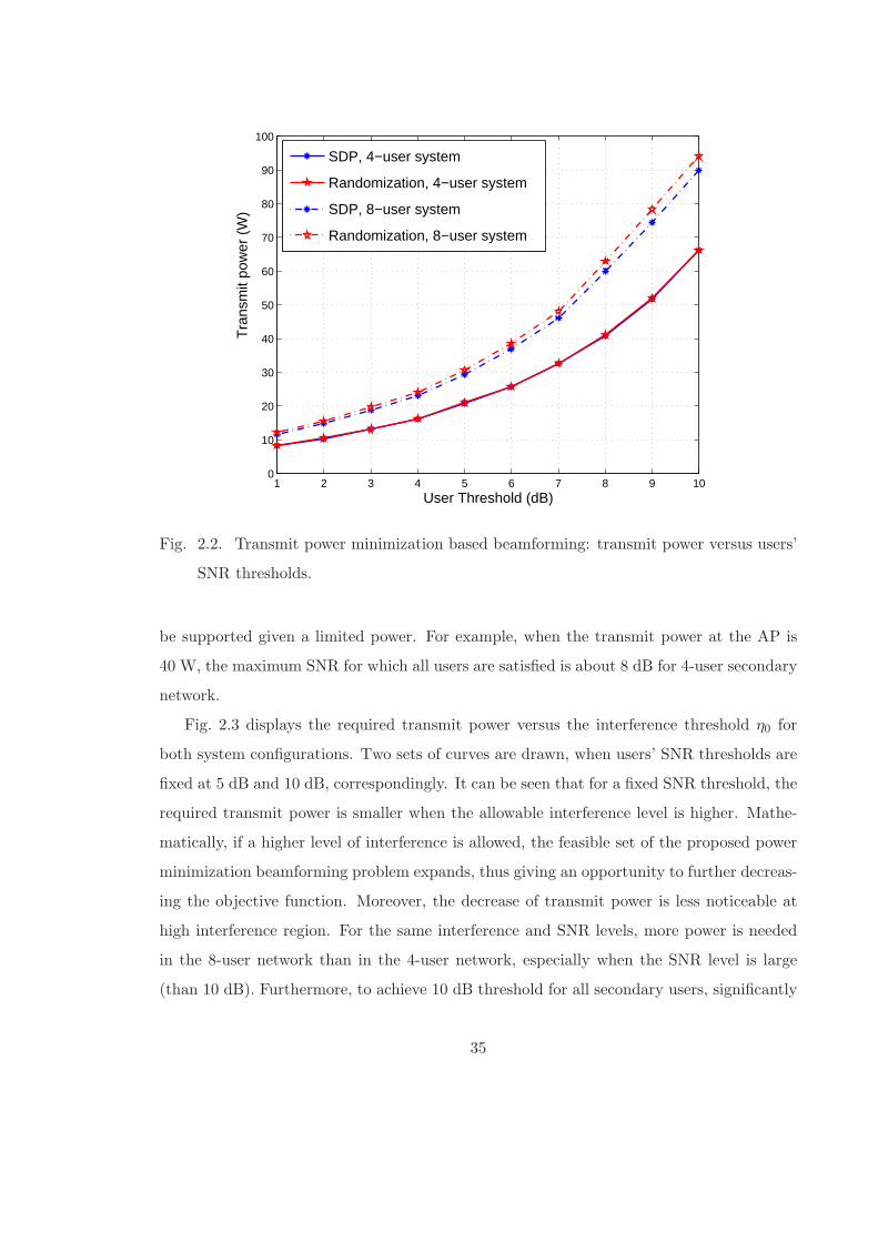
1 2 3 4 5 6 7 8 9 100
10
20
30
40
50
60
70
80
90
100
User Threshold (dB)
Tra
nsm
it po
wer
(W
)
SDP, 4−user system
Randomization, 4−user system
SDP, 8−user system
Randomization, 8−user system
Fig. 2.2. Transmit power minimization based beamforming: transmit power versus users’
SNR thresholds.
be supported given a limited power. For example, when the transmit power at the AP is
40 W, the maximum SNR for which all users are satisfied is about 8 dB for 4-user secondary
network.
Fig. 2.3 displays the required transmit power versus the interference threshold η0 for
both system configurations. Two sets of curves are drawn, when users’ SNR thresholds are
fixed at 5 dB and 10 dB, correspondingly. It can be seen that for a fixed SNR threshold, the
required transmit power is smaller when the allowable interference level is higher. Mathe-
matically, if a higher level of interference is allowed, the feasible set of the proposed power
minimization beamforming problem expands, thus giving an opportunity to further decreas-
ing the objective function. Moreover, the decrease of transmit power is less noticeable at
high interference region. For the same interference and SNR levels, more power is needed
in the 8-user network than in the 4-user network, especially when the SNR level is large
(than 10 dB). Furthermore, to achieve 10 dB threshold for all secondary users, significantly
35
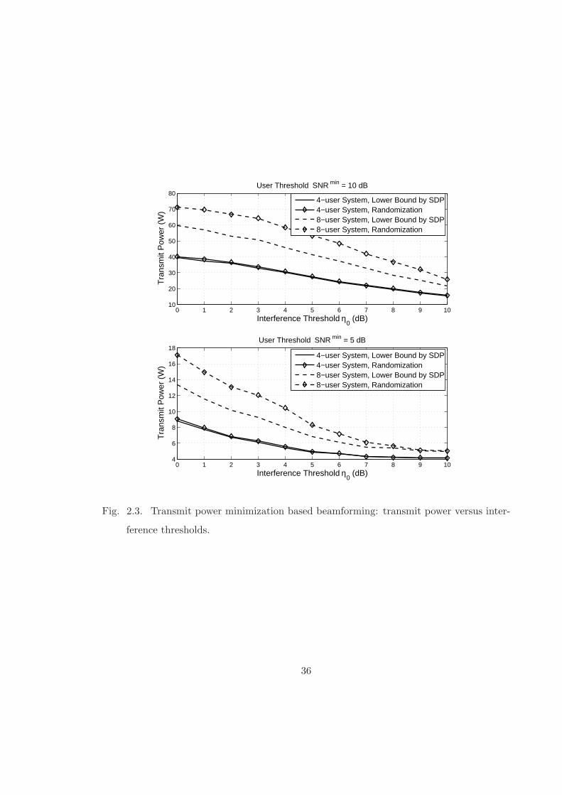
0 1 2 3 4 5 6 7 8 9 1010
20
30
40
50
60
70
80
Interference Threshold η0 (dB)
Tra
nsm
it P
ower
(W
)
User Threshold SNR min = 10 dB
0 1 2 3 4 5 6 7 8 9 104
6
8
10
12
14
16
18
Interference Threshold η0 (dB)
Tra
nsm
it P
ower
(W
)
User Threshold SNR min = 5 dB
4−user System, Lower Bound by SDP4−user System, Randomization8−user System, Lower Bound by SDP8−user System, Randomization
4−user System, Lower Bound by SDP4−user System, Randomization8−user System, Lower Bound by SDP8−user System, Randomization
Fig. 2.3. Transmit power minimization based beamforming: transmit power versus inter-
ference thresholds.
36
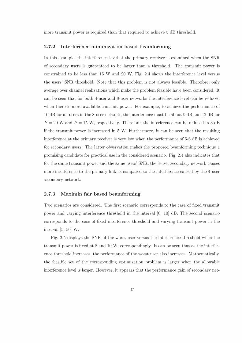
more transmit power is required than that required to achieve 5 dB threshold.
2.7.2 Interference minimization based beamforming
In this example, the interference level at the primary receiver is examined when the SNR
of secondary users is guaranteed to be larger than a threshold. The transmit power is
constrained to be less than 15 W and 20 W. Fig. 2.4 shows the interference level versus
the users’ SNR threshold. Note that this problem is not always feasible. Therefore, only
average over channel realizations which make the problem feasible have been considered. It
can be seen that for both 4-user and 8-user networks the interference level can be reduced
when there is more available transmit power. For example, to achieve the performance of
10 dB for all users in the 8-user network, the interference must be about 9 dB and 12 dB for
P = 20 W and P = 15 W, respectively. Therefore, the interference can be reduced in 3 dB
if the transmit power is increased in 5 W. Furthermore, it can be seen that the resulting
interference at the primary receiver is very low when the performance of 5-6 dB is achieved
for secondary users. The latter observation makes the proposed beamforming technique a
promising candidate for practical use in the considered scenario. Fig. 2.4 also indicates that
for the same transmit power and the same users’ SNR, the 8-user secondary network causes
more interference to the primary link as compared to the interference caused by the 4-user
secondary network.
2.7.3 Maximin fair based beamforming
Two scenarios are considered. The first scenario corresponds to the case of fixed transmit
power and varying interference threshold in the interval [0, 10] dB. The second scenario
corresponds to the case of fixed interference threshold and varying transmit power in the
interval [5, 50] W.
Fig. 2.5 displays the SNR of the worst user versus the interference threshold when the
transmit power is fixed at 8 and 10 W, correspondingly. It can be seen that as the interfer-
ence threshold increases, the performance of the worst user also increases. Mathematically,
the feasible set of the corresponding optimization problem is larger when the allowable
interference level is larger. However, it appears that the performance gain of secondary net-
37
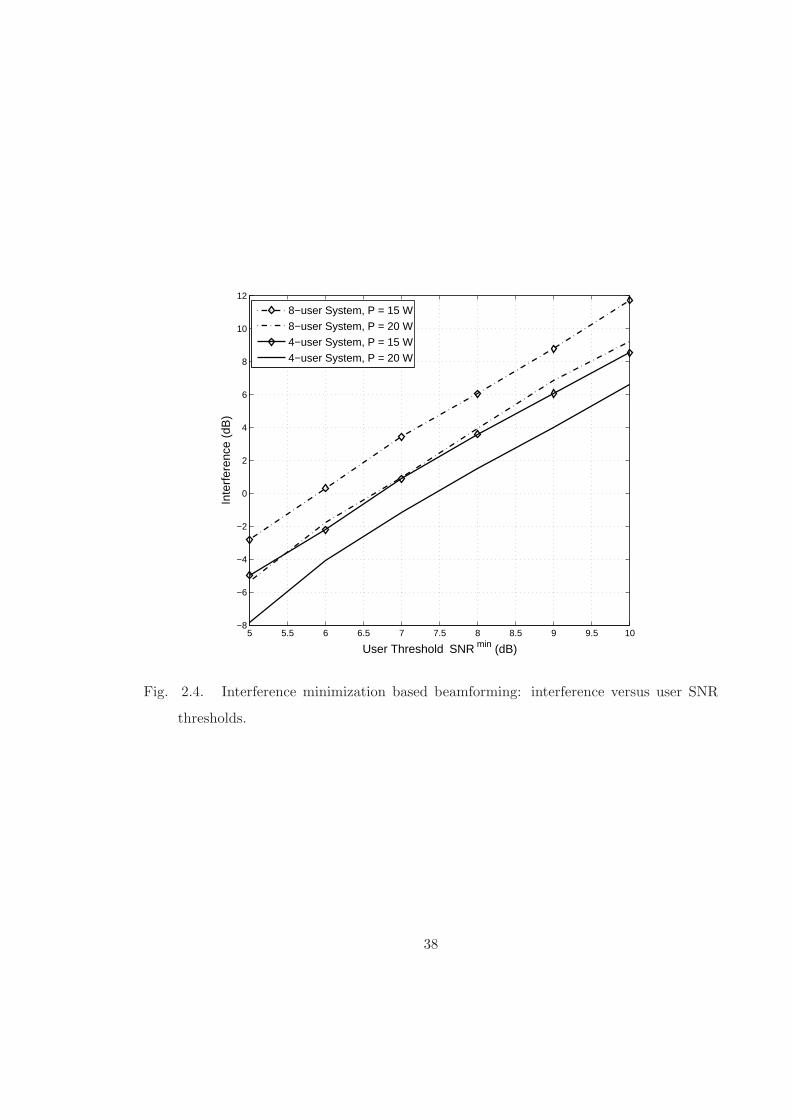
5 5.5 6 6.5 7 7.5 8 8.5 9 9.5 10−8
−6
−4
−2
0
2
4
6
8
10
12
User Threshold SNR min (dB)
Inte
rfer
ence
(dB
)
8−user System, P = 15 W
8−user System, P = 20 W
4−user System, P = 15 W
4−user System, P = 20 W
Fig. 2.4. Interference minimization based beamforming: interference versus user SNR
thresholds.
38
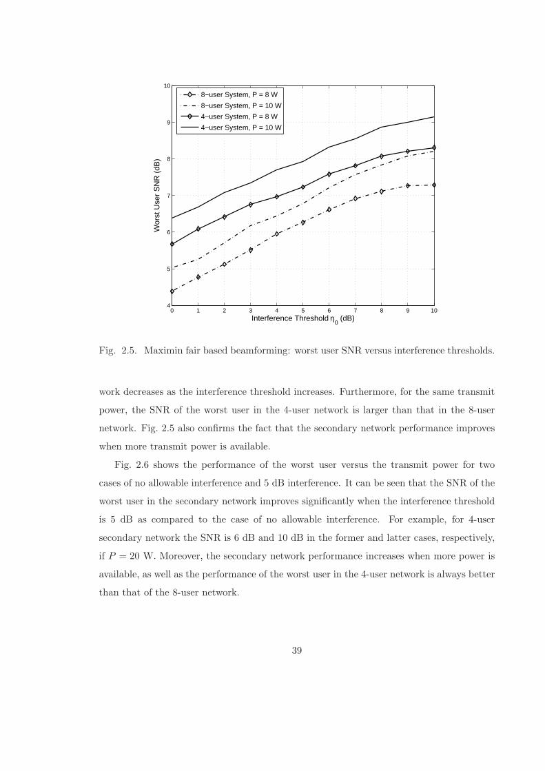
0 1 2 3 4 5 6 7 8 9 104
5
6
7
8
9
10
Interference Threshold η0 (dB)
Wor
st U
ser
SN
R (
dB)
8−user System, P = 8 W
8−user System, P = 10 W
4−user System, P = 8 W
4−user System, P = 10 W
Fig. 2.5. Maximin fair based beamforming: worst user SNR versus interference thresholds.
work decreases as the interference threshold increases. Furthermore, for the same transmit
power, the SNR of the worst user in the 4-user network is larger than that in the 8-user
network. Fig. 2.5 also confirms the fact that the secondary network performance improves
when more transmit power is available.
Fig. 2.6 shows the performance of the worst user versus the transmit power for two
cases of no allowable interference and 5 dB interference. It can be seen that the SNR of the
worst user in the secondary network improves significantly when the interference threshold
is 5 dB as compared to the case of no allowable interference. For example, for 4-user
secondary network the SNR is 6 dB and 10 dB in the former and latter cases, respectively,
if P = 20 W. Moreover, the secondary network performance increases when more power is
available, as well as the performance of the worst user in the 4-user network is always better
than that of the 8-user network.
39
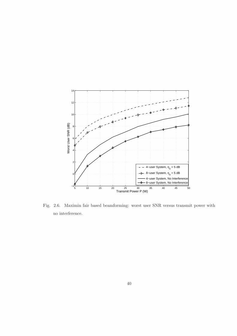
5 10 15 20 25 30 35 40 45 50−2
0
2
4
6
8
10
12
14
Transmit Power P (W)
Wor
st U
ser
SN
R (
dB)
4−user System, η0 = 5 dB
8−user System, η0 = 5 dB
4−user System, No Interference8−user System, No Interference
Fig. 2.6. Maximin fair based beamforming: worst user SNR versus transmit power with
no interference.
40
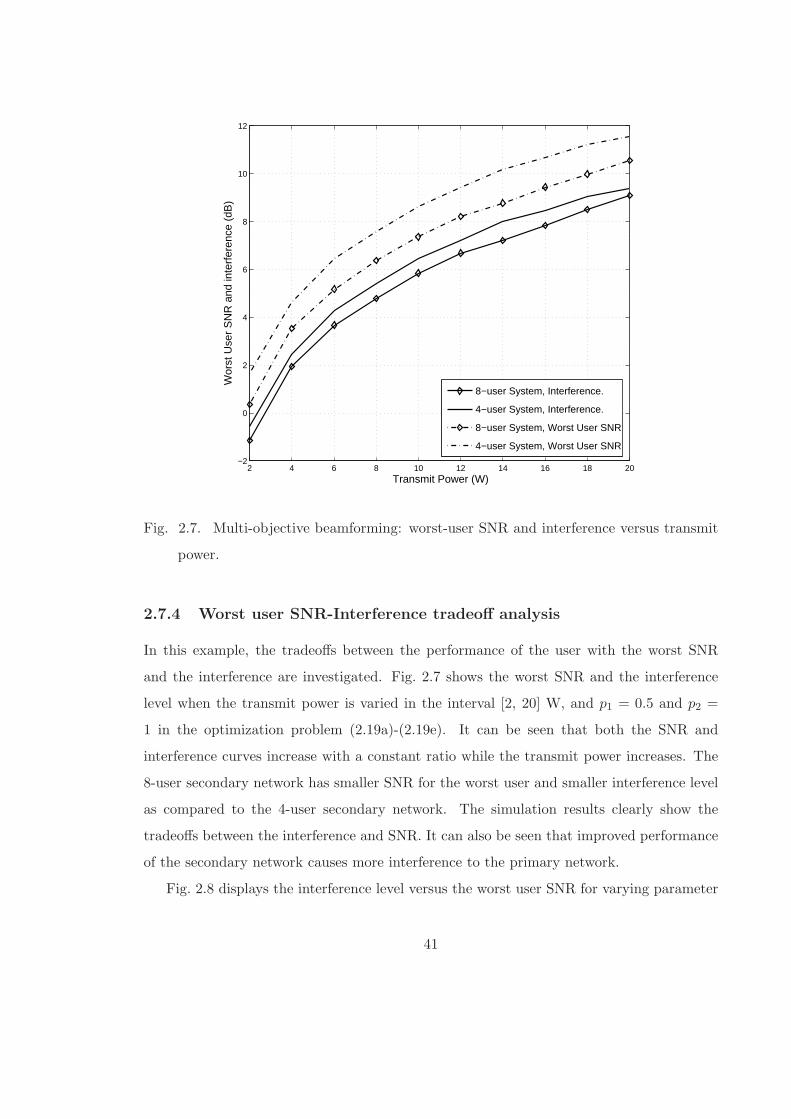
2 4 6 8 10 12 14 16 18 20−2
0
2
4
6
8
10
12
Transmit Power (W)
Wor
st U
ser
SN
R a
nd in
terf
eren
ce (
dB)
8−user System, Interference.
4−user System, Interference.
8−user System, Worst User SNR
4−user System, Worst User SNR
Fig. 2.7. Multi-objective beamforming: worst-user SNR and interference versus transmit
power.
2.7.4 Worst user SNR-Interference tradeoff analysis
In this example, the tradeoffs between the performance of the user with the worst SNR
and the interference are investigated. Fig. 2.7 shows the worst SNR and the interference
level when the transmit power is varied in the interval [2, 20] W, and p1 = 0.5 and p2 =
1 in the optimization problem (2.19a)-(2.19e). It can be seen that both the SNR and
interference curves increase with a constant ratio while the transmit power increases. The
8-user secondary network has smaller SNR for the worst user and smaller interference level
as compared to the 4-user secondary network. The simulation results clearly show the
tradeoffs between the interference and SNR. It can also be seen that improved performance
of the secondary network causes more interference to the primary network.
Fig. 2.8 displays the interference level versus the worst user SNR for varying parameter
41
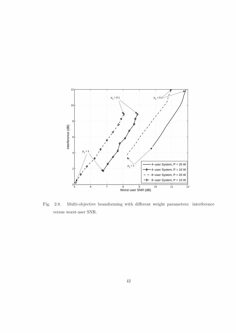
5 6 7 8 9 10 11 120
2
4
6
8
10
12
Worst user SNR (dB)
Inte
rfer
ence
(dB
)
4−user System, P = 20 W
4−user System, P = 10 W
8−user System, P = 20 W
8−user System, P = 10 W
p1 = 0.1 p
1 = 0.1
p1 = 1
p1 = 1
Fig. 2.8. Multi-objective beamforming with different weight parameters: interference
versus worst-user SNR.
42
p1 in the interval [0.1, 1], while the parameter p2 is fixed and equals to 1, and the transmit
power is fixed at 10 W and 20 W. It should be noted that for smaller p1, the proposed
multi-objective beamforming tries to improve the worst user SNR, while for large p1 it tries
to suppress interference. It can be seen in Fig. 2.8 that for p1 = 0.1, the interference is
indeed the largest and the worst user SNR is the largest, while for p1 = 1, the worst user
SNR is the smallest and the interference is the smallest. Fig. 2.8 shows that the interaction
between those two metrics depends on the weight factors that are set for each objective.
2.8 Conclusions
Problem formulations and solution approaches for multicast beamforming for secondary
wireless networks have been developed. Using the CSI available at the transmitter, the QoS
for both primary and secondary users can be effectively controlled. Therefore, the network of
secondary users is able to operate simultaneously with the network of primary users without
any need for channel sensing. In particular, a number of practically important design
scenarios with different criteria involving the interference level at the primary receivers, the
received SNR of the secondary users and the transmit power have been considered. Although
the proposed designs are nonconvex and NP-hard, a convex relaxation approach coupled
with suitable randomization post-processing provides approximate solutions at a moderate
computational cost that is strictly bounded by a low-order polynomial. Our approach
can also be applicable in conventional cellular systems when broadcasting to a number of
receivers and at the same time protecting some specific ‘directions’ from interference.
43
Chapter 3
Power Allocation in Wireless
Multi-user Relay Networks
WE CONSIDER IN THIS CHAPTER AN AMPLIFY-and-FORWARD (AF) wireless
relay network where multiple source nodes communicate with their corresponding
destination nodes with the help of relay nodes. While each user1 is assisted by one relay,
one relay can assist many users. Conventionally, each relay node is assumed to equally
distribute the available communication resources to all sources for which it helps to relay
information. This approach is clearly sub-optimal since each user experiences dissimilar
channel conditions, and thus, demanding different amount of allocated resources to meet its
QoS requirements. For that reason, this work presents novel power allocation schemes to
i) maximize the minimum end-to-end signal-to-noise ratio among all users; ii) minimize the
total transmit power over all sources; iii) maximize the network throughput. Moreover, due
to limited power resource, even with optimal power allocation, it may happen to be not pos-
sible to satisfy QoS requirements for all users. As a result, an admission control algorithm
should be carried out to maximize the number of users that can be served. Depending on
the set of admitted users, optimal power allocation is then performed. Because of its com-
binatorial hardness, the joint optimal admission control and power allocation problem has
high complexity to compute the solution. Therefore, an efficient heuristic-based algorithm
1Hereafter, the term ’user’ refers to a source-destination pair or only the source node depending on the
context.
44
is developed for solving the aforementioned problem with significantly reduced complexity.
Although theoretically sub-optimal, the devised algorithm performs remarkably well. The
proposed power allocation problems are formulated using GP, a well-studied class of non-
linear and nonconvex optimization problems. Since GP problem is readily transformed into
an equivalent convex optimization problem, optimal solution can be obtained efficiently.
Numerical results demonstrate the effectiveness of our proposed approach.
The rest of this chapter is organized as follows. Section 3.1 overviews the literature
review on resource allocation for wireless relay networks and summarizes our contributions.
In Section 3.2, a multi-user wireless relay model with multiple relays is described. Section 3.3
contains the problem formulations for three different power control schemes. The proposed
problems are converted into GP problems in Section 3.4. The problem of joint admission
control and power allocation is presented in Section 3.5. The algorithm for solving the
joint admission control and power allocation problem is described in Section 3.6. Numerical
examples are presented in Section 3.7, followed by the conclusions in Section 3.8.
3.1 Introduction
3.1.1 Literature review
Recently, it has been shown that the operation efficiency and QoS of cellular and/or ad-
hoc networks can be increased through the use of relay(s) [8], [9]. In such systems, the
information from the source to the corresponding destination is transmitted via a direct-
link and also forwarded via relays. Due to its significant advances, for example, coverage
extension and performance improvement, relay-assisted communications can be seen as a
candidate for the deployment of future generation networks. Although various relay system
models have been proposed and studied, the conventional two-hop relay model has attracted
much research attention [8], [9], [44], [45], [46]. This is because it is viable to implement
such systems in practice. The performance of a two-hop relay system is investigated for
various channel models, i.e., Rayleigh or Nakagami-m, and relaying models, i.e., AF or
decode-and-forward (DF). Note, however, that resource allocation is assumed to be fixed in
these works.
Another critical issue for improving the performance of wireless networks is efficient
45
management of available radio resources [4], [5]. Specifically, resource allocation via power
control is commonly used. Furthermore, in relay networks, appropriate power allocation
among the participating nodes helps to ensure the performance and stability of the system.
As a result, there have been numerous works which attempt to optimize the available
communication resources, i.e., power and bandwidth to improve the system performance
[47], [48], [49], [50], [51], [52]. It is worth mentioning that a single source-destination pair
is typically considered in the aforementioned papers. In [47], for example, the authors
derive closed-form expressions for the optimal and near-optimal relay transmission powers
for the single relay and the multiple relays cases, respectively. Both AF and DF relaying
scenarios are considered. The problem of minimizing the transmission power given that a
target outage probability is achieved was tackled in [48]. In [49], the authors derive power
allocation strategies for 3-node AF relaying system based on the knowledge of channel
means. The performance criteria used are either the SNR gain or the outage probability. An
information theoretic analysis for a similar system model with Rayleigh fading and CSI at
the transmitter side is carried out in [50] where the upper and lower bounds on the channel
capacity are derived. Optimal power allocation scheme is also studied. The bandwidth
allocation problem in 3-node Gaussian orthogonal relay channel is also investigated in [51].
The optimization parameter which represents the fraction of the bandwidth assigned to
source-relay channel is computed to maximize a lower bound on the capacity. Given either
full CSI of the links or channel statistics, [52] presents two power allocation schemes to
minimize the outage probability. A cross-layer optimization framework, i.e., congestion
control, routing, relay selection and power allocation via dual decomposition for multihop
networks using cooperative diversity is proposed in [53].
3.1.2 Motivation and contributions
It should be noted that very few works have considered the aforementioned 2-hop relay
model for more practical case of multiple users.2 Therefore, the above-mentioned analy-
sis is applicable to only a special case of the problem under consideration. Indeed, each
2Note that multi-user cooperative network employing orthogonal frequency-division multiple-access
(OFDMA) where subscribers can relay information for each other is already considered, for example
see [54], [55] and references therein.
46
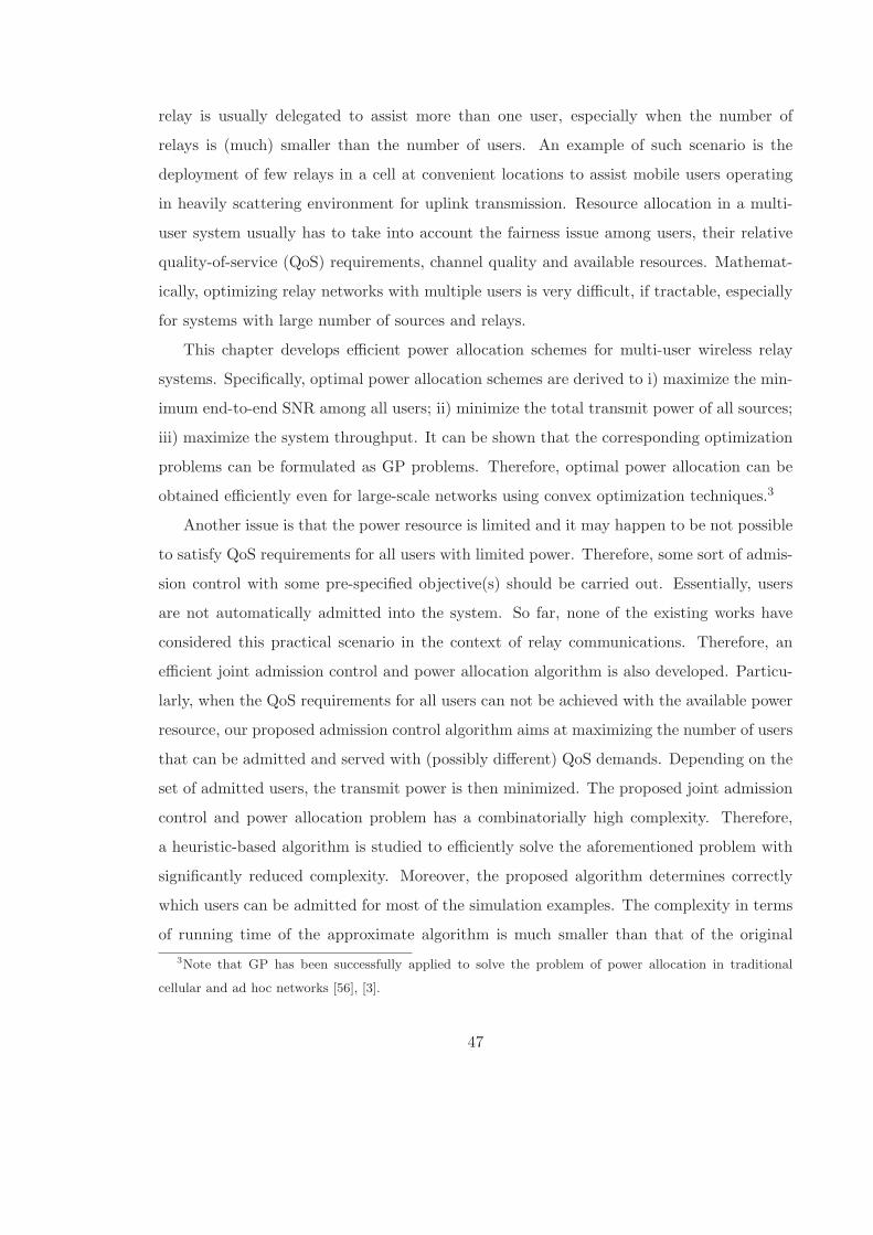
relay is usually delegated to assist more than one user, especially when the number of
relays is (much) smaller than the number of users. An example of such scenario is the
deployment of few relays in a cell at convenient locations to assist mobile users operating
in heavily scattering environment for uplink transmission. Resource allocation in a multi-
user system usually has to take into account the fairness issue among users, their relative
quality-of-service (QoS) requirements, channel quality and available resources. Mathemat-
ically, optimizing relay networks with multiple users is very difficult, if tractable, especially
for systems with large number of sources and relays.
This chapter develops efficient power allocation schemes for multi-user wireless relay
systems. Specifically, optimal power allocation schemes are derived to i) maximize the min-
imum end-to-end SNR among all users; ii) minimize the total transmit power of all sources;
iii) maximize the system throughput. It can be shown that the corresponding optimization
problems can be formulated as GP problems. Therefore, optimal power allocation can be
obtained efficiently even for large-scale networks using convex optimization techniques.3
Another issue is that the power resource is limited and it may happen to be not possible
to satisfy QoS requirements for all users with limited power. Therefore, some sort of admis-
sion control with some pre-specified objective(s) should be carried out. Essentially, users
are not automatically admitted into the system. So far, none of the existing works have
considered this practical scenario in the context of relay communications. Therefore, an
efficient joint admission control and power allocation algorithm is also developed. Particu-
larly, when the QoS requirements for all users can not be achieved with the available power
resource, our proposed admission control algorithm aims at maximizing the number of users
that can be admitted and served with (possibly different) QoS demands. Depending on the
set of admitted users, the transmit power is then minimized. The proposed joint admission
control and power allocation problem has a combinatorially high complexity. Therefore,
a heuristic-based algorithm is studied to efficiently solve the aforementioned problem with
significantly reduced complexity. Moreover, the proposed algorithm determines correctly
which users can be admitted for most of the simulation examples. The complexity in terms
of running time of the approximate algorithm is much smaller than that of the original
3Note that GP has been successfully applied to solve the problem of power allocation in traditional
cellular and ad hoc networks [56], [3].
47
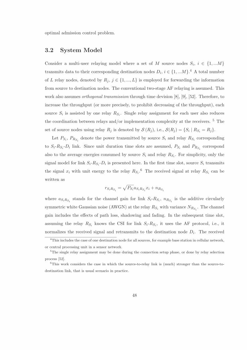
optimal admission control problem.
3.2 System Model
Consider a multi-user relaying model where a set of M source nodes Si, i ∈ {1, ...M}transmits data to their corresponding destination nodes Di, i ∈ {1, ...M}.4 A total number
of L relay nodes, denoted by Rj , j ∈ {1, ..., L} is employed for forwarding the information
from source to destination nodes. The conventional two-stage AF relaying is assumed. This
work also assumes orthogonal transmission through time devision [8], [9], [52]. Therefore, to
increase the throughput (or more precisely, to prohibit decreasing of the throughput), each
source Si is assisted by one relay RSi. Single relay assignment for each user also reduces
the coordination between relays and/or implementation complexity at the receivers. 5 The
set of source nodes using relay Rj is denoted by S (Rj), i.e., S(Rj) = {Si | RSi= Rj}.
Let PSi, PRSi
denote the power transmitted by source Si and relay RSicorresponding
to Si-RSi-Di link. Since unit duration time slots are assumed, PSi
and PRSicorrespond
also to the average energies consumed by source Si and relay RSi. For simplicity, only the
signal model for link Si-RSi-Di is presented here. In the first time slot, source Si transmits
the signal xi with unit energy to the relay RSi.6 The received signal at relay RSi
can be
written as
rSiRSi=√
PSiaSiRSi
xi + nRSi
where aSiRSistands for the channel gain for link Si-RSi
, nRSiis the additive circularly
symmetric white Gaussian noise (AWGN) at the relay RSiwith variance NRSi
. The channel
gain includes the effects of path loss, shadowing and fading. In the subsequent time slot,
assuming the relay RSiknows the CSI for link Si-RSi
, it uses the AF protocol, i.e., it
normalizes the received signal and retransmits to the destination node Di. The received
4This includes the case of one destination node for all sources, for example base station in cellular network,
or central processing unit in a sensor network.5The single relay assignment may be done during the connection setup phase, or done by relay selection
process [52].6This work considers the case in which the source-to-relay link is (much) stronger than the source-to-
destination link, that is usual scenario in practice.
48
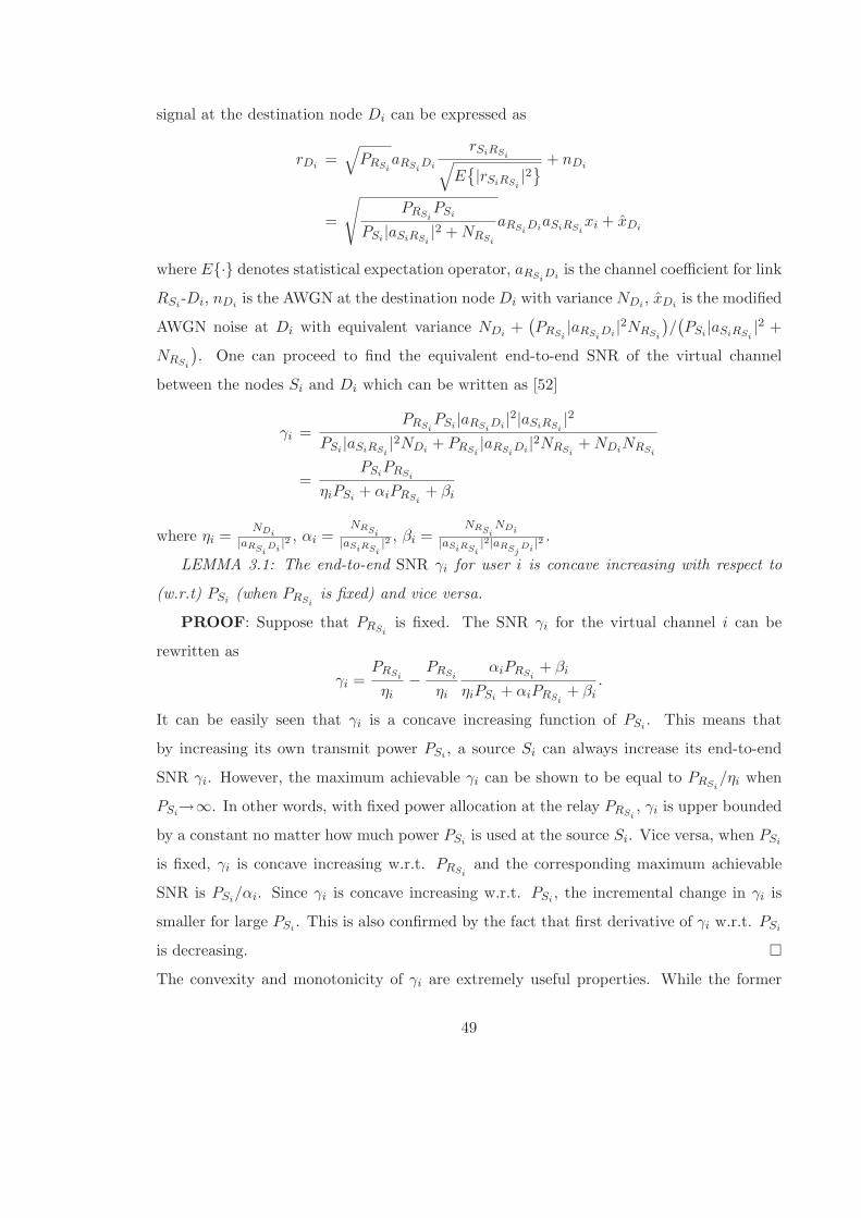
signal at the destination node Di can be expressed as
rDi=√
PRSiaRSi
Di
rSiRSi√
E{
|rSiRSi|2}
+ nDi
=
√
PRSiPSi
PSi|aSiRSi
|2 + NRSi
aRSiDi
aSiRSixi + xDi
where E{·} denotes statistical expectation operator, aRSiDi
is the channel coefficient for link
RSi-Di, nDi
is the AWGN at the destination node Di with variance NDi, xDi
is the modified
AWGN noise at Di with equivalent variance NDi+(
PRSi|aRSi
Di|2NRSi
)
/(
PSi|aSiRSi
|2 +
NRSi
)
. One can proceed to find the equivalent end-to-end SNR of the virtual channel
between the nodes Si and Di which can be written as [52]
γi =PRSi
PSi|aRSi
Di|2|aSiRSi
|2PSi
|aSiRSi|2NDi
+ PRSi|aRSi
Di|2NRSi
+ NDiNRSi
=PSi
PRSi
ηiPSi+ αiPRSi
+ βi
where ηi =NDi
|aRSiDi
|2, αi =
NRSi
|aSiRSi|2
, βi =NRSi
NDi
|aSiRSi|2|aRSj
Di|2
.
LEMMA 3.1: The end-to-end SNR γi for user i is concave increasing with respect to
(w.r.t) PSi(when PRSi
is fixed) and vice versa.
PROOF: Suppose that PRSiis fixed. The SNR γi for the virtual channel i can be
rewritten as
γi =PRSi
ηi−
PRSi
ηi
αiPRSi+ βi
ηiPSi+ αiPRSi
+ βi.
It can be easily seen that γi is a concave increasing function of PSi. This means that
by increasing its own transmit power PSi, a source Si can always increase its end-to-end
SNR γi. However, the maximum achievable γi can be shown to be equal to PRSi/ηi when
PSi→∞. In other words, with fixed power allocation at the relay PRSi
, γi is upper bounded
by a constant no matter how much power PSiis used at the source Si. Vice versa, when PSi
is fixed, γi is concave increasing w.r.t. PRSiand the corresponding maximum achievable
SNR is PSi/αi. Since γi is concave increasing w.r.t. PSi
, the incremental change in γi is
smaller for large PSi. This is also confirmed by the fact that first derivative of γi w.r.t. PSi
is decreasing. �
The convexity and monotonicity of γi are extremely useful properties. While the former
49
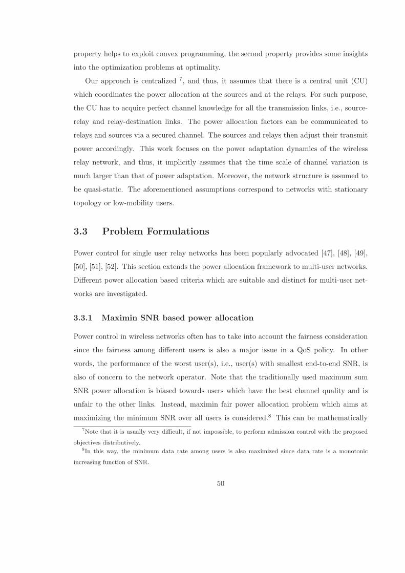
property helps to exploit convex programming, the second property provides some insights
into the optimization problems at optimality.
Our approach is centralized 7, and thus, it assumes that there is a central unit (CU)
which coordinates the power allocation at the sources and at the relays. For such purpose,
the CU has to acquire perfect channel knowledge for all the transmission links, i.e., source-
relay and relay-destination links. The power allocation factors can be communicated to
relays and sources via a secured channel. The sources and relays then adjust their transmit
power accordingly. This work focuses on the power adaptation dynamics of the wireless
relay network, and thus, it implicitly assumes that the time scale of channel variation is
much larger than that of power adaptation. Moreover, the network structure is assumed to
be quasi-static. The aforementioned assumptions correspond to networks with stationary
topology or low-mobility users.
3.3 Problem Formulations
Power control for single user relay networks has been popularly advocated [47], [48], [49],
[50], [51], [52]. This section extends the power allocation framework to multi-user networks.
Different power allocation based criteria which are suitable and distinct for multi-user net-
works are investigated.
3.3.1 Maximin SNR based power allocation
Power control in wireless networks often has to take into account the fairness consideration
since the fairness among different users is also a major issue in a QoS policy. In other
words, the performance of the worst user(s), i.e., user(s) with smallest end-to-end SNR, is
also of concern to the network operator. Note that the traditionally used maximum sum
SNR power allocation is biased towards users which have the best channel quality and is
unfair to the other links. Instead, maximin fair power allocation problem which aims at
maximizing the minimum SNR over all users is considered.8 This can be mathematically
7Note that it is usually very difficult, if not impossible, to perform admission control with the proposed
objectives distributively.8In this way, the minimum data rate among users is also maximized since data rate is a monotonic
increasing function of SNR.
50
posed as
maxPSi
, PRSi
mini=1,...,M
γi(PSi, PRSi
) (3.1a)
subject to:∑
Si∈S(Rj)
PRSi≤ Pmax
Rj, j = 1, . . . , L (3.1b)
M∑
i=1
PSi≤ P (3.1c)
0 ≤ PSi≤ Pmax
Si, ∀Si, i ∈ {1, ...M} (3.1d)
where PmaxRj
is the total power available at the relay node Rj and P is the total power
allocated to all sources. The right-hand side of (3.1b) is the total power that the relay Rj
allocates to the users which it assists and it is constrained to be less than the relay’s total
power. The constraints (3.1d) specify the peak power limit PmaxSi
for each source Si. Note
that the constraint (3.1c) is necessary in this case since otherwise, sources Si, ∀i would
transmit with their maximum power. Moreover, the constraint (3.1c) assumes that the
sources can be coordinated to share the power resource.
LEMMA 3.2: The optimization problem (3.1a)–(3.1c) is feasible. Moreover, to obtain
maximum performance for the system, the inequality constraints (3.1b), (3.1c) must be met
with equality at optimality.
PROOF: Clearly, the constraint set is compact and nonempty, and thus, the opti-
mization problem (3.1a)–(3.1c) is feasible. Using contradiction, we suppose that P ∗S =
[P ∗S1
, . . . , P ∗SM
]T , P ∗R = [P ∗
RS1, . . . , P ∗
RSM]T are the optimal power allocation of the sources
and relays respectively. First, it can be shown that the constraint (3.1c) must be achieved
with equality. If it is not, P ∗S can be scaled by a factor α > 1 which is determined by
α =P
∑Mi=1 P ∗
Si
> 1
i.e., P+S = αP ∗
S . It is clear that the power allocation P+S , P ∗
R is also feasible. This power
allocation will improve the objective function since each of γi is an increasing function w.r.t.
PSi, or equivalently mini=1,...,M γi is increasing w.r.t. PSi
. This contradicts the optimality
assumption. This completes the proof. �
For all users to achieve their maximum performance, the constraints (3.1b) should also
be met with equality. Using similar argument, suppose that the constraint associated with
51
relay Rj is not met with equality at optimality. One then can scale P ∗RSi
, Si ∈ S (Rj) by a
factor greater than 1 and show that the new power allocation is also feasible. This power
allocation will improve the SNR of the users which the relay Rj assists. If the worst user(s)
is assisted by Rj , its performance will be improved. Otherwise, the performance of the
worst user(s) is not affected.
It can be seen that, although the end-to-end performance of user i depends only on
‘local’ power allocation i.e., PSiand PRSi
, the performance of users interact with each other
via the constraints on the available resources. Therefore, resource allocation in a multi-user
network is not as simple as allocating resources for each user individually, albeit orthogonal
transmissions are assumed.
3.3.2 Transmit power minimization based power allocation
In practical wireless networks, one of the targets of power allocation is to prolong the lifetime
of battery-powered devices since nodes with long lifetime help to ensure uninterrupted
information exchange. Commonly, to achieve better performance, the source itself transmits
at its maximum available power as Lemma 3.1 reveals. As a result, the energy may run out
quickly. However, since each user has a minimum QoS requirement in terms of SNR, by
taking into account the optimal power allocation at the relays, the source node might not
need to transmit at its largest power level. Therefore, sources save their power and prolong
its lifetime. Since the relay nodes are usually energy-unlimited devices, this problem exploits
the available power at the relay nodes to save power at the battery-powered source nodes.
The transmit power minimization problem subject to constraints on the end-to-end SNR
for each user can be formulated as follows
minPSi
, PRSi
M∑
i=1
PSi(3.2a)
subject to: γi ≥ γmini , i = 1, . . . , M (3.2b)
The constraints (3.1b), (3.1d) (3.2c)
where γmini is the threshold SNR for ith user.9 It can be seen that the optimization problem
(3.2a)–(3.2c) is also always feasible. The power constraints (3.1b) in (3.2c) are used to pro-
9In this problem formulation, it assumes that the threshold γmini is not larger than the maximum achiev-
able SNR for user i as discussed in Lemma 3.1.
52
hibit a situation when some particular relays are allocating too much power to the user(s).
The resulting optimal power allocation obviously can require some sources to transmit more
power than the others. Therefore, additionally, a weighted sum of powers, or the maximum
user power can be minimized. A practical application of the power optimization problem
(3.2a)–(3.2c) is in the stage of network planning for wireless mesh or ad hoc networks.
LEMMA 3.3: At optimality, the inequality constraints (3.2b), (3.1b) in (3.2c) of the
problem (3.2a)–(3.2c) must be met with equality.
PROOF: It can be proved using the monotonicity of the γi w.r.t. PSiand PRSi
.
Specifically, since γi is increasing w.r.t. PSiand PRSi
, in order to minimize PSi, PRSi
must
attain its possible maximum value. Likewise, γi must attain its possible minimum value to
minimize PSi. Therefore, the inequalities (3.2b), (3.1b) in (3.2c) must be met with equality
at optimality. �
3.3.3 Network throughput maximization based power allocation
The maximin based power allocation aim at improving the system performance by improving
the performance of the worst user. On the other hand, it is well-known that in order to
achieve maximin rate fairness among users, there is a loss in the system throughput, i.e., the
users sum rate. For some applications, for example, applications which require high data
rate transmission from any user, the system throughput with optimal power allocation is
desirable. Users with good channel quality can transmit faster and users with bad channel
quality can transmit slower. Moreover, the network throughput, in the case of perfect CSI
and optimal power allocation, defines the upper bound on the system achievable rates.
Given the end-to-end SNR γi of user i, the data rate Ri can be written as a function of γi
as follows
Ri =1
Tlog2(1 + Kγi) ≈
1
Tlog2(Kγi)
where T is the symbol period which is assumed to be equal to 1 for brevity, K = −ζi
ln(ζ2BER) ,
BER is the target bit error rate, and ζ1, ζ2 are constants dependent on the modulation
scheme [57]. Note that 1 + Kγi has been approximated as Kγi which is reasonable when
Kγi is much larger than 1. For notational simplicity in the rest of the chapter, K is set to
53
be equal to 1. Then, the network aggregate throughput can be written as [3]
R =
M∑
i=1
Ri = log2
[
M∏
i=1
γi
]
.
The power allocation problem to maximize the network throughput can be mathematically
posed as
maxPSi
, PRSi
R = log2
[
M∏
i=1
γi
]
(3.3a)
subject to: The constraints (3.1b), (3.1c), (3.1d). (3.3b)
Note that in the high SNR region, the problem of maximizing network throughout is equiv-
alent to that of maximizing the product of SNRs. Here, no lower constraint on the data
rate for each user is assumed. However, these constraints can be incorporated easily, and
they will not change the GP structure of the problems. Moreover, the achievable network
throughput in this case will be less than that of (3.3a)–(3.3b) due to smaller feasible set.
LEMMA 3.4: At optimality, the inequality constraints (3.3b) of the problem (3.3a)–
(3.3b) must be met with equality.
PROOF: The proof can be constructed similarly as the proof of Lemma 3.3.
Note that the throughput maximization based power allocation (3.3a)–(3.3b) does not
penalize users with “bad” channels and favor users with “good” channels. Interesting that
the system throughput maximization criterion in the power control techniques for cellular
networks usually results in the situation when some users are prevented from transmitting
data [3]. However in our case, as Lemma 3.1 suggests, the SNR γi for a particular user i is
concave increasing function of allocated powers, that is, the incremental change in SNR is
smaller for larger transmit power. In Fig. 3.1, SNRs are plotted versus allocated power at
the relays when source powers are fixed and equal. It can be seen that instead of allocating
more power to the users with “good” channel conditions at high SNR, the proposed scheme
allocates power to the users with “bad” channel conditions at low SNR. It results in im-
provement in the sum throughput of the network as compared to the conventional power
allocation schemes in cellular networks, because the performance of the users with “bad”
channel conditions is not severely affected. This fact is also confirmed in the simulation
section.
54
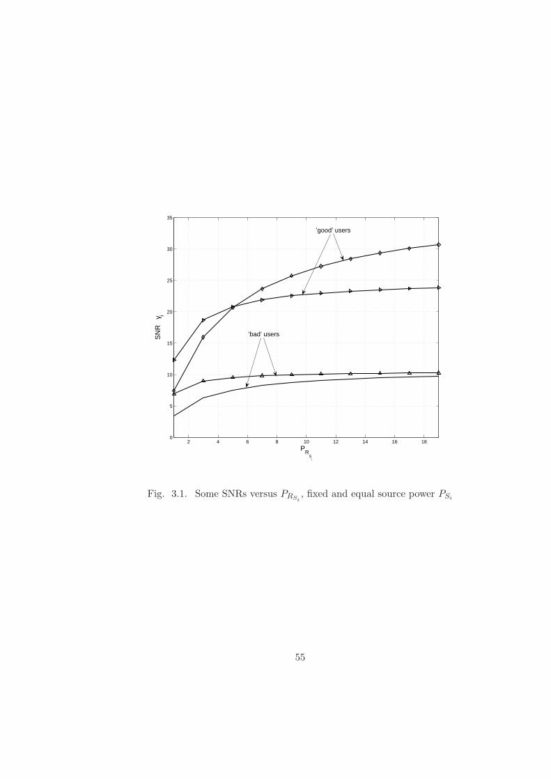
2 4 6 8 10 12 14 16 180
5
10
15
20
25
30
35
PR
Si
SN
R
γ i
’good’ users
’bad’ users
Fig. 3.1. Some SNRs versus PRSi, fixed and equal source power PSi
55
3.4 Power Allocation in Relay Networks via GP
GP is a well-investigated class of nonlinear, nonconvex optimization problems with attrac-
tive theoretical and computational properties [56], [3]. Since equivalent convex reformulation
is possible for a GP problem, there exist no local optimum points but only global optimum.
Moreover, the availability of large-scale software solvers makes GP more appealing.
3.4.1 Maximin SNR based power allocation
Introducing a new slack variable t, one can equivalently rewrite the optimization problem
(3.1a)–(3.1c) as follows
minPSi
, PRSi, t≥0
1
t(3.4a)
subject to:PSi
PRSi
ηiPSi+ αiPRSi
+ βi≥ t, i = 1, . . . , M (3.4b)
The constraints (3.1b), (3.1c), (3.1d). (3.4c)
The objective function of the problem (3.4a)–(3.4c) is a monomial function. Moreover,
the constraints in (3.4b) can be easily converted into posynomial constraints. The con-
straints (3.1b), (3.1c), (3.1d) are linear w.r.t. the power variables, and thus, are posynomial
constraints. Therefore, the optimization problem (3.4a)–(3.4c) is the GP problem.
3.4.2 Transmit power minimization based power allocation
In this case, the objective function is clearly a posynomial function. The constraints can
be written as posynomial ones. Therefore, the power minimization based power allocation
is the GP problem.
3.4.3 Network throughput maximization based power allocation
A simple manipulation of the optimization problem (3.3a)–(3.3b) gives
minPSi
, PRSi
1∏M
i=1 γi
(3.5a)
subject to: The constraints (3.1b), (3.1c), (3.1d). (3.5b)
56
Each of the terms 1/γi is a posynomial in PSiand PRSi
, and the product of posynomials
is also a posynomial. Therefore, the optimization problem (3.5a)–(3.5b) also belongs to
the GP class. 10 As maximizing aggregate throughput can be extremely unfair to some
users, a weighted sum of data rates, i.e.,∑M
i=1 wiRi where wi is a given weight coefficient
for user i, can be used an objective function to be maximized. Using some manipulations,
the resulting optimization problem can be reformulated as a GP problem as well.
It has been shown that all three aforementioned power allocation schemes can be re-
formulated as GP problems. The proposed optimization problems with distinct features
of relaying model are mathematically similar to the ones in [3] for conventional cellular
network. However, the numerator and denominator of the SNR expression for each user
considered in [3] are linear functions of the power variables which is not the case in our
work.
3.5 Joint Admission Control and Power Allocation
It is well-known that one of the important resource management issues is the determination
of which users to establish connections. Then, communications resources are to be assigned
to connected users to ensure that each connected user has an acceptable signal quality [58].
Traditionally, each user has a minimum QoS requirement that needs to be satisfied. Due to
the fact that wireless communication systems are usually resource-limited, they are typically
unable to meet all users’ QoS requirements. As a result, users are not certainly admitted.
In other words, only a limited number of users can be admitted into the system. Our
admission control algorithm determines which users can be served concurrently. Then, the
power allocation is used to minimize the transmit power.
3.5.1 A revised transmit power minimization based power allocation
As mentioned above, the problem formulation (3.2a)–(3.2c) is always feasible as long as
γmini , ∀i is less than the maximum achievable value. This is because the sources have been
10Note that the high operating SNR region is assumed. If medium or low SIR regions are assumed, the
approximation 1 + Kγi by Kγi may not be accurate. In this case, successive convex approximation method
as in [3] can be used. However, it is out of the scope of this work.
57
assumed to be able to transmit as much power as possible to increase their end-to-end
SNRs. However, this is clearly impractical in power-limited systems. Therefore, the power
minimization based allocation problem (3.2a)–(3.2c) incorporating the power constraint can
be re-expressed as follows
minPSi
, PRSi
M∑
i=1
PSi(3.6a)
subject to: γi ≥ γmini , i = 1, . . . , M (3.6b)
∑
Si∈S(Rj)
PRSi≤ Pmax
Rj, j = 1, . . . , L (3.6c)
M∑
i=1
PSi≤ P (3.6d)
0 ≤ PSi≤ Pmax
Si, ∀Si, i ∈ {1, . . . , M}. (3.6e)
There are instances when the optimization problem (3.6a)–(3.6e) becomes infeasible.
For example, it is likely to be infeasible when SNR targets γmini are too high, or simply
when the number of users M is large. Clearly, the channel quality also affects the feasibility
of (3.6a)–(3.6e). It can be seen that infeasibility happens due to the power limits of both the
relays and/or the sources. A practical implication of the infeasibility is that it is impossible
to serve (admit) all M users at their desired QoS requirements. Some approaches to the
infeasible problem can be however used. For example, some users can be dropped or the
SNR targets could be relaxed, i.e., made smaller. This work investigates the former scenario
and try to maximize the number of users that can be served at their desired QoS.
3.5.2 A mathematical framework for joint admission control and power
allocation problem
The joint admission control and power allocation problem can be mathematically stated as
a 2-stage optimization problem [59]. In the first stage, one finds a set S0 of users such that
S0 = arg maxS⊆{1,...,M}, PSi
, PRSi
|S| (3.7a)
subject to: γi ≥ γmini , i ∈ S (3.7b)
The constraints (3.6c), (3.6d), (3.6e) (3.7c)
58
where |S| denotes the cardinality of S. Given the optimal set of admitted users S0, in the
second stage, the required transmit power at the relays is minimized. The second stage
optimization can be written as
minPSi
, PRSi
M∑
i=1
PSi(3.8a)
subject to: γi ≥ γmini , i ∈ S0 (3.8b)
The constraints (3.6c), (3.6d), (3.6e). (3.8c)
Alternatively, the joint admission control and power minimization can be regarded as a
bilevel programming problem. The more difficult part is the admission control problem
which is combinatorially hard. Once the set of admitted users are determined, the power
minimization problem can be shown to be a convex programming problem. Due to its com-
binatorial hardness, the joint admission control and power allocation problem admits high
complexity for practical implementation. In the following section, an efficient algorithm for
solving sub-optimally (3.7a)–(3.7c) and (3.8a)–(3.8c) with significantly reduced complexity
is proposed.
3.6 Proposed Algorithm
3.6.1 A reformulation of joint admission control and power allocation
problem
A brute-force way of doing admission control (3.7a)–(3.7c) involves exhaustively solving
all subsets of users which has high complexity.11 Therefore, a better way of solving the
problem of joint admission control-power allocation is highly desirable. It can be shown
that the admission control problem (3.7a)–(3.7c) can be mathematically recast using the
indicator variables si, i = 1, . . . , M , i.e, si = 0, si = 1 means that user i is not admitted,
or otherwise, respectively. The following theorem is in order.
11In practice, it may not need to search all the sets of users to find the optimal solution.
59
THEOREM 3.1: The aforementioned 2-stage optimization problem (3.7a)–(3.7c), (3.8a)–
(3.8c) is equivalent to the following 1-stage optimization problem
maxsi∈{0,1}, PSi
, PRSi
ǫ
M∑
i=1
si − (1 − ǫ)
M∑
i=1
PSi(3.9a)
subject to: γi ≥ γmini si, i = 1, . . . , M (3.9b)
The constraints (3.6c), (3.6d), (3.6e) (3.9c)
where ǫ is some constant that is chosen such that P/(P + 1) < ǫ < 1..
PROOF: The proof is a 2-step process. First, one needs to prove that the optimization
problem (3.9a)–(3.9c) extracts the maximum number of possibly admitted users. Second,
among all sets of maximum possibly admitted users, solving (3.9a)–(3.9c) gives the set of
users which requires least total power.
Suppose that S∗0 , P ∗
Si, P ∗
RSiare the admitted users and power allocated to users at
the corresponding relays 12, respectively obtained by solving (3.9a)–(3.9c), and |S∗0 | = n∗.
Thus, the optimal value of the objective function is L∗ = ǫn∗ − (1 − ǫ)∑M
i=1 P ∗Si
. Suppose
that there is another feasible solution S+0 , P+
Si, P+
RSisuch that |S+
0 | = n+ > n∗ with the
objective value L+ = ǫn+ − (1 − ǫ)∑M
i=1 P+Si
. One has
L+−L∗ = ǫ(n+ − n∗) + (1 − ǫ)
(
M∑
i=1
P ∗Si
−M∑
i=1
P+Si
)
≥ ǫ − (1 − ǫ)P > 0. (3.10)
The first inequality corresponds to the assumption that n+ − n∗ ≥ 1 and the fact that
∣
∣
∣
M∑
i=1
P ∗Si
−M∑
i=1
P+Si
∣
∣
∣≤ P.
The second inequality is due the choice of ǫ > PP+1 . This obviously contradicts the as-
sumption that S∗0 , P ∗
Si, P ∗
RSiare optimal solutions. Therefore, by solving (3.9a)–(3.9c), one
obtains the largest set of users that can be served at their desired QoS with the available
power. In other words, users are dropped only when necessary.
In the second step, it needs to be proved that among the sets with equal maximum
possibly admitted users, solving (3.9a)–(3.9c) gives the minimum transmit power. Again,
12The optimal set of admitted users is S∗
0 = {i | s∗i = 1}.
60
suppose that S†0, P †
Si, P †
RSiis another feasible solution such that |S†
0| = n∗ with the objective
value L† = ǫn∗ − (1 − ǫ)∑M
i=1 P †Si
. Since S∗0 , P ∗
Si, P ∗
RSiare the optimal solutions to the
problem (3.9a)–(3.9c), L† < L∗. Therefore, it can be concluded that∑M
i=1 P ∗Si
<∑M
i=1 P †Si
.
This completes the proof. �
Note that the problem formulation (3.9a)–(3.9c) is similar to a multi-objective optimiza-
tion problem, i.e., maximization of the number of admitted users and minimization of the
transmit power, with ǫ being the priority for the former criterion. Therefore, it is reasonable
to set ǫ large to maximize number of admitted users as a priority.
LEMMA 3.5: The optimization problem (3.9a)–(3.9c) is always feasible.
PROOF: It is easy to see that no users are admitted in the worst case, i.e., si = 0, ∀i =
1, . . . , N . In this case, the problem is always feasible. �
The indicator variables help to represent the admission control problem in a more com-
pact mathematical form. However, the combinatorial nature of the admission control prob-
lem still exists due to the binary variables si. To this end, it should be mentioned that the
optimization problem (3.9a)–(3.9c) is extremely hard, if not impossible, to solve. It belongs
to the class of nonconvex integer optimization problems. Even when the binary variables si
are relaxed to be continuous, the resulting optimization problem is also nonconvex. This is
a subtle difference compared to the optimization in [59]. Therefore, we propose a reduced-
complexity heuristic algorithm to perform admission control and power allocation. Albeit
theoretical sub-optimal, its performance is remarkably close to that of the optimal solution
for most of the testing instances.
3.6.2 Proposed algorithm
As discussed above, once the difficult admission control part is solved, the problem of
minimizing the transmit power boils down to a convex programming problem. The following
heuristic algorithm can be used to solve (3.9a)–(3.9c).13
• Step 1. Set S := {Si | i = 1, . . . , M}.
• Step 2. Solve GP problem (3.6a)–(3.6e) without the constraint (3.6e) for the
sources in S. Let P ∗Si
, P ∗RSi
denote the resulting power allocation values.
13It should be noted that more efficient may be developed.
61
• Step 3. If∑
Si∈S P ∗Si
≤ P , then stop and P ∗Si
, P ∗RSi
being power allocation values.
Otherwise, user Si with largest required power value, i.e., Si = arg maxSi∈S
{
P ∗Si
}
is
removed from S and go to step 2.
It can be seen that after each iteration, either the set of admitted users and the cor-
responding power allocation levels are determined or one user is removed from the list of
most possibly admitted users. Since there are M initial users, the complexity is bounded
above by that of solving M GP problems with different dimensions. It is worth mentioning
that the proposed reduced complexity algorithm always returns one solution.
3.7 Simulation Results
To demonstrate the effectiveness of the proposed power allocation schemes, consider a wire-
less relay network as in Fig. 3.2 with 10 users and 3 relays distributed in a two-dimensional
region 200m×200m. The relays are fixed at coordinates (100,50), (100,100), and (100,150).
The 10 source nodes and their corresponding destination nodes are deployed randomly in
the area inside the box area [(0, 0), (50, 200)] and [(150, 0), (200, 200)], respectively. In our
simulation, each source is assisted by a random (and then fixed) relay. No microscopic
fading is assumed and the gain for each transmission link is computed using the path loss
model as a = 1/d where d is the Euclidean distance between two transmission ends. The
noise power at the receiver ends is assumed to be identical and equals to N0 = −50 dB.
Although each relay node may assist different number of users, they are assumed to have the
same maximum power level PmaxRj
. Similarly, all users are assumed to have equal minimum
SNR thresholds γmin. The software package [12] has been used for solving convex programs
in our simulations.
3.7.1 Power allocation without admission control
Fig. 3.3 and Fig. 3.4 show the minimum rate among all users and the network throughput
i.e., sum of users’ rates when the maximum power levels of the relays PmaxRj
and sources P are
varied. The performance of the equal power allocation (EPA) scheme is also plotted. In this
case, the power is allocated equally among all sources, i.e., PSi= P/10, ∀Si and each relay
distributes power equally among all users which it assists. For P = 50 (see Fig. 3.3), the
62
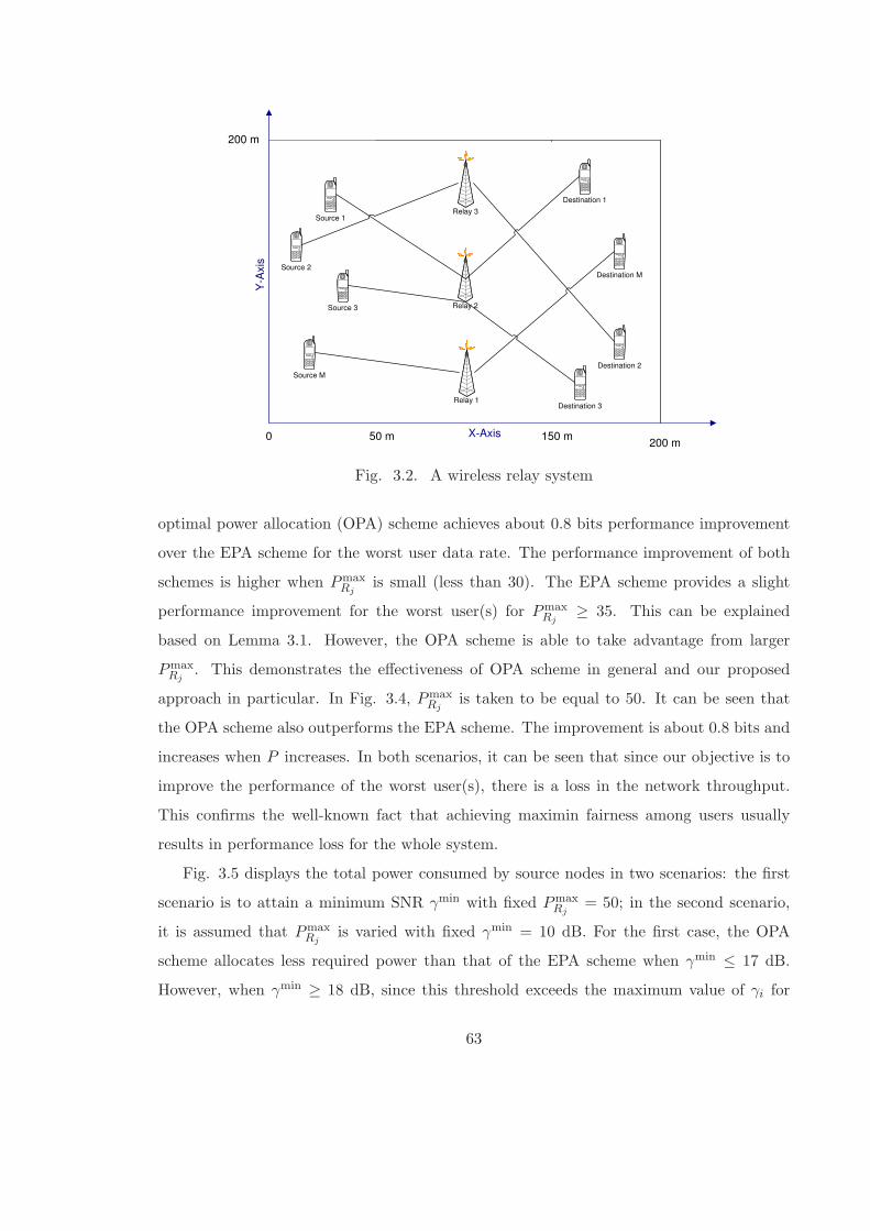
Source 1
Source M
Relay 3
Relay 1
Y-A
xis
X-Axis
200 m
200 m0 50 m 150 m
Relay 2
Source 2
Source 3
Destination M
Destination 2
Destination 3
Destination 1
Fig. 3.2. A wireless relay system
optimal power allocation (OPA) scheme achieves about 0.8 bits performance improvement
over the EPA scheme for the worst user data rate. The performance improvement of both
schemes is higher when PmaxRj
is small (less than 30). The EPA scheme provides a slight
performance improvement for the worst user(s) for PmaxRj
≥ 35. This can be explained
based on Lemma 3.1. However, the OPA scheme is able to take advantage from larger
PmaxRj
. This demonstrates the effectiveness of OPA scheme in general and our proposed
approach in particular. In Fig. 3.4, PmaxRj
is taken to be equal to 50. It can be seen that
the OPA scheme also outperforms the EPA scheme. The improvement is about 0.8 bits and
increases when P increases. In both scenarios, it can be seen that since our objective is to
improve the performance of the worst user(s), there is a loss in the network throughput.
This confirms the well-known fact that achieving maximin fairness among users usually
results in performance loss for the whole system.
Fig. 3.5 displays the total power consumed by source nodes in two scenarios: the first
scenario is to attain a minimum SNR γmin with fixed PmaxRj
= 50; in the second scenario,
it is assumed that PmaxRj
is varied with fixed γmin = 10 dB. For the first case, the OPA
scheme allocates less required power than that of the EPA scheme when γmin ≤ 17 dB.
However, when γmin ≥ 18 dB, since this threshold exceeds the maximum value of γi for
63
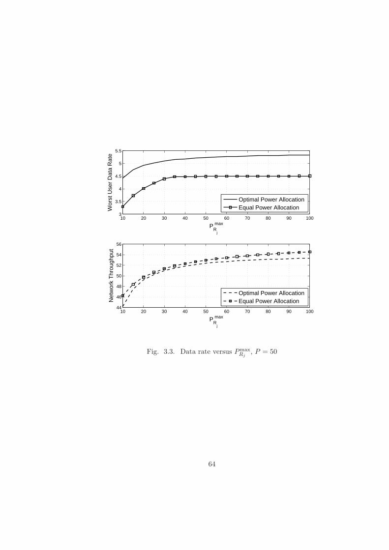
10 20 30 40 50 60 70 80 90 1003
3.5
4
4.5
5
5.5
PR
j
max
Wor
st U
ser
Dat
a R
ate
10 20 30 40 50 60 70 80 90 10044
46
48
50
52
54
56
PR
j
max
Net
wor
k T
hrou
ghpu
t
Optimal Power AllocationEqual Power Allocation
Optimal Power AllocationEqual Power Allocation
Fig. 3.3. Data rate versus PmaxRj
, P = 50
64
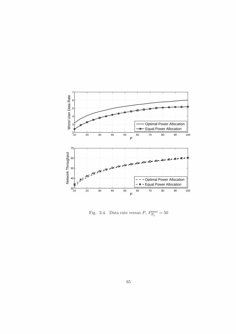
10 20 30 40 50 60 70 80 90 1002
3
4
5
6
7
P
Wor
st U
ser
Dat
a R
ate
10 20 30 40 50 60 70 80 90 10030
40
50
60
70
P
Net
wor
k T
hrou
ghpu
t
Optimal Power AllocationEqual Power Allocation
Optimal Power AllocationEqual Power Allocation
Fig. 3.4. Data rate versus P , PmaxRj
= 50
65
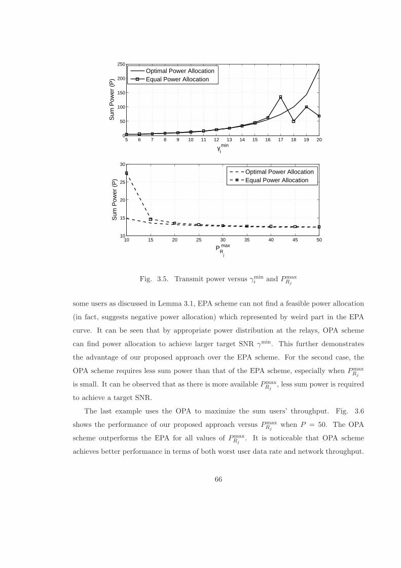
5 6 7 8 9 10 11 12 13 14 15 16 17 18 19 200
50
100
150
200
250
γi min
Sum
Pow
er (
P)
10 15 20 25 30 35 40 45 5010
15
20
25
30
PR
j
max
Sum
Pow
er (
P)
Optimal Power AllocationEqual Power Allocation
Optimal Power AllocationEqual Power Allocation
Fig. 3.5. Transmit power versus γmini and Pmax
Rj
some users as discussed in Lemma 3.1, EPA scheme can not find a feasible power allocation
(in fact, suggests negative power allocation) which represented by weird part in the EPA
curve. It can be seen that by appropriate power distribution at the relays, OPA scheme
can find power allocation to achieve larger target SNR γmin. This further demonstrates
the advantage of our proposed approach over the EPA scheme. For the second case, the
OPA scheme requires less sum power than that of the EPA scheme, especially when PmaxRj
is small. It can be observed that as there is more available PmaxRj
, less sum power is required
to achieve a target SNR.
The last example uses the OPA to maximize the sum users’ throughput. Fig. 3.6
shows the performance of our proposed approach versus PmaxRj
when P = 50. The OPA
scheme outperforms the EPA for all values of PmaxRj
. It is noticeable that OPA scheme
achieves better performance in terms of both worst user data rate and network throughput.
66
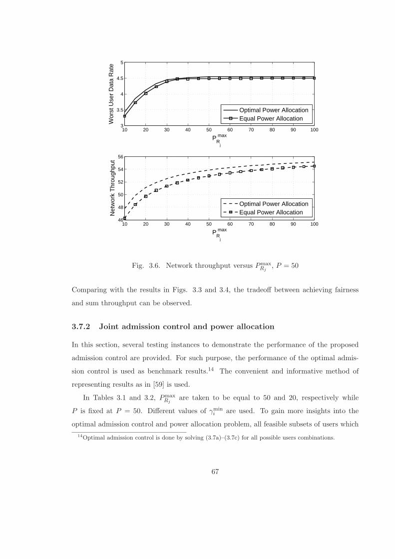
10 20 30 40 50 60 70 80 90 1003
3.5
4
4.5
5
PR
j
max
Wor
st U
ser
Dat
a R
ate
10 20 30 40 50 60 70 80 90 10046
48
50
52
54
56
PR
j
max
Net
wor
k T
hrou
ghpu
t
Optimal Power AllocationEqual Power Allocation
Optimal Power AllocationEqual Power Allocation
Fig. 3.6. Network throughput versus PmaxRj
, P = 50
Comparing with the results in Figs. 3.3 and 3.4, the tradeoff between achieving fairness
and sum throughput can be observed.
3.7.2 Joint admission control and power allocation
In this section, several testing instances to demonstrate the performance of the proposed
admission control are provided. For such purpose, the performance of the optimal admis-
sion control is used as benchmark results.14 The convenient and informative method of
representing results as in [59] is used.
In Tables 3.1 and 3.2, PmaxRj
are taken to be equal to 50 and 20, respectively while
P is fixed at P = 50. Different values of γmini are used. To gain more insights into the
optimal admission control and power allocation problem, all feasible subsets of users which
14Optimal admission control is done by solving (3.7a)–(3.7c) for all possible users combinations.
67
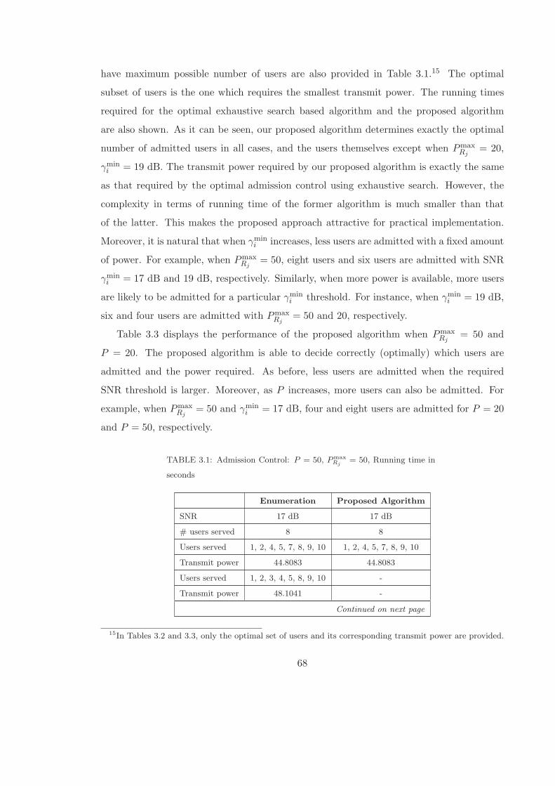
have maximum possible number of users are also provided in Table 3.1.15 The optimal
subset of users is the one which requires the smallest transmit power. The running times
required for the optimal exhaustive search based algorithm and the proposed algorithm
are also shown. As it can be seen, our proposed algorithm determines exactly the optimal
number of admitted users in all cases, and the users themselves except when PmaxRj
= 20,
γmini = 19 dB. The transmit power required by our proposed algorithm is exactly the same
as that required by the optimal admission control using exhaustive search. However, the
complexity in terms of running time of the former algorithm is much smaller than that
of the latter. This makes the proposed approach attractive for practical implementation.
Moreover, it is natural that when γmini increases, less users are admitted with a fixed amount
of power. For example, when PmaxRj
= 50, eight users and six users are admitted with SNR
γmini = 17 dB and 19 dB, respectively. Similarly, when more power is available, more users
are likely to be admitted for a particular γmini threshold. For instance, when γmin
i = 19 dB,
six and four users are admitted with PmaxRj
= 50 and 20, respectively.
Table 3.3 displays the performance of the proposed algorithm when PmaxRj
= 50 and
P = 20. The proposed algorithm is able to decide correctly (optimally) which users are
admitted and the power required. As before, less users are admitted when the required
SNR threshold is larger. Moreover, as P increases, more users can also be admitted. For
example, when PmaxRj
= 50 and γmini = 17 dB, four and eight users are admitted for P = 20
and P = 50, respectively.
TABLE 3.1: Admission Control: P = 50, PmaxRj
= 50, Running time in
seconds
Enumeration Proposed Algorithm
SNR 17 dB 17 dB
# users served 8 8
Users served 1, 2, 4, 5, 7, 8, 9, 10 1, 2, 4, 5, 7, 8, 9, 10
Transmit power 44.8083 44.8083
Users served 1, 2, 3, 4, 5, 8, 9, 10 -
Transmit power 48.1041 -
Continued on next page
15In Tables 3.2 and 3.3, only the optimal set of users and its corresponding transmit power are provided.
68
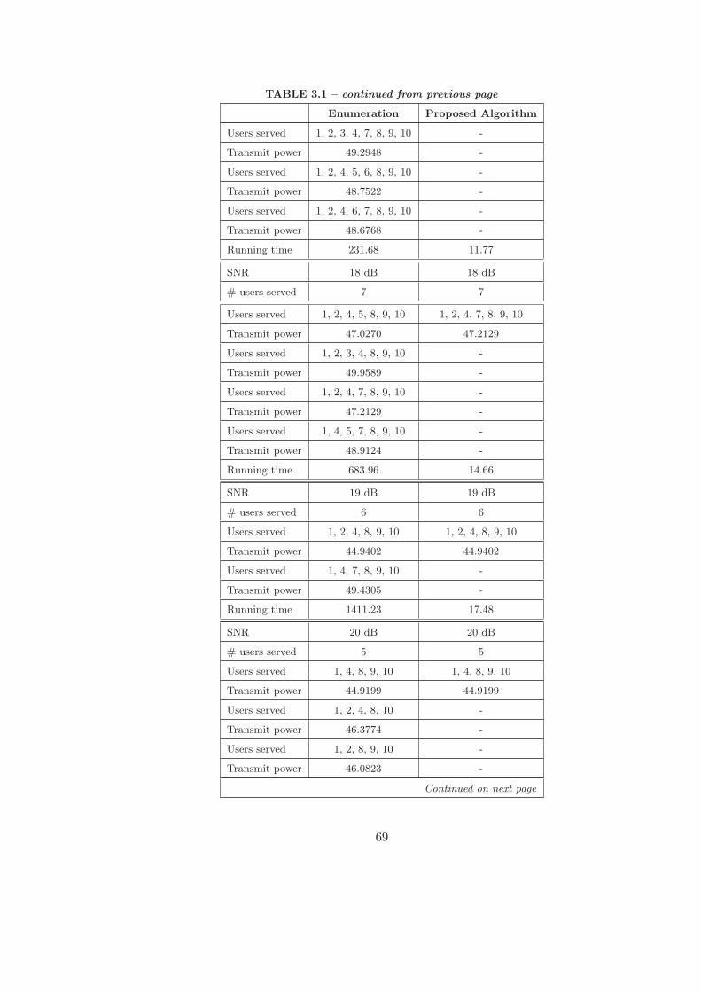
TABLE 3.1 – continued from previous page
Enumeration Proposed Algorithm
Users served 1, 2, 3, 4, 7, 8, 9, 10 -
Transmit power 49.2948 -
Users served 1, 2, 4, 5, 6, 8, 9, 10 -
Transmit power 48.7522 -
Users served 1, 2, 4, 6, 7, 8, 9, 10 -
Transmit power 48.6768 -
Running time 231.68 11.77
SNR 18 dB 18 dB
# users served 7 7
Users served 1, 2, 4, 5, 8, 9, 10 1, 2, 4, 7, 8, 9, 10
Transmit power 47.0270 47.2129
Users served 1, 2, 3, 4, 8, 9, 10 -
Transmit power 49.9589 -
Users served 1, 2, 4, 7, 8, 9, 10 -
Transmit power 47.2129 -
Users served 1, 4, 5, 7, 8, 9, 10 -
Transmit power 48.9124 -
Running time 683.96 14.66
SNR 19 dB 19 dB
# users served 6 6
Users served 1, 2, 4, 8, 9, 10 1, 2, 4, 8, 9, 10
Transmit power 44.9402 44.9402
Users served 1, 4, 7, 8, 9, 10 -
Transmit power 49.4305 -
Running time 1411.23 17.48
SNR 20 dB 20 dB
# users served 5 5
Users served 1, 4, 8, 9, 10 1, 4, 8, 9, 10
Transmit power 44.9199 44.9199
Users served 1, 2, 4, 8, 10 -
Transmit power 46.3774 -
Users served 1, 2, 8, 9, 10 -
Transmit power 46.0823 -
Continued on next page
69
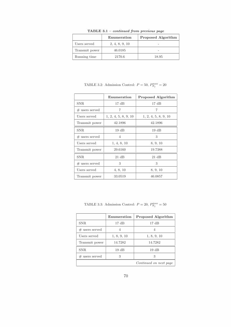
TABLE 3.1 – continued from previous page
Enumeration Proposed Algorithm
Users served 2, 4, 8, 9, 10 -
Transmit power 46.0185 -
Running time 2170.6 18.95
TABLE 3.2: Admission Control: P = 50, PmaxRj
= 20
Enumeration Proposed Algorithm
SNR 17 dB 17 dB
# users served 7 7
Users served 1, 2, 4, 5, 8, 9, 10 1, 2, 4, 5, 8, 9, 10
Transmit power 42.1896 42.1896
SNR 19 dB 19 dB
# users served 4 3
Users served 1, 4, 8, 10 8, 9, 10
Transmit power 29.6160 19.7388
SNR 21 dB 21 dB
# users served 3 3
Users served 4, 8, 10 8, 9, 10
Transmit power 33.0519 46.0857
TABLE 3.3: Admission Control: P = 20, PmaxRj
= 50
Enumeration Proposed Algorithm
SNR 17 dB 17 dB
# users served 4 4
Users served 1, 8, 9, 10 1, 8, 9, 10
Transmit power 14.7282 14.7282
SNR 19 dB 19 dB
# users served 3 3
Continued on next page
70
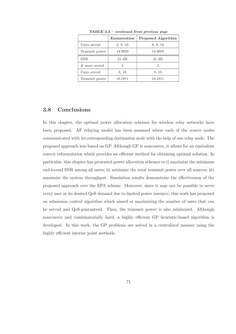
TABLE 3.3 – continued from previous page
Enumeration Proposed Algorithm
Users served 8, 9, 10 8, 9, 10
Transmit power 14.9059 14.9059
SNR 21 dB 21 dB
# users served 2 2
Users served 8, 10 8, 10
Transmit power 10.1811 10.1811
3.8 Conclusions
In this chapter, the optimal power allocation schemes for wireless relay networks have
been proposed. AF relaying model has been assumed where each of the source nodes
communicated with its corresponding destination node with the help of one relay node. The
proposed approach was based on GP. Although GP is nonconvex, it allows for an equivalent
convex reformulation which provides an efficient method for obtaining optimal solution. In
particular, this chapter has presented power allocation schemes to i) maximize the minimum
end-to-end SNR among all users; ii) minimize the total transmit power over all sources; iii)
maximize the system throughput. Simulation results demonstrate the effectiveness of the
proposed approach over the EPA scheme. Moreover, since it may not be possible to serve
every user at its desired QoS demand due to limited power resource, this work has proposed
an admission control algorithm which aimed at maximizing the number of users that can
be served and QoS-guaranteed. Then, the transmit power is also minimized. Although
nonconvex and combinatorially hard, a highly efficient GP heuristic-based algorithm is
developed. In this work, the GP problems are solved in a centralized manner using the
highly efficient interior point methods.
71
Chapter 4
Joint Medium Access Control,
Routing and Energy Distribution
in Multi-Hop Wireless Networks
IT IS A CHALLENGING TASK TO PROVIDE end-to-end QoS provisioning in multi-hop
wireless networks which involves a cross-layer optimization. This chapter presents a joint
cross-layer optimization approach, i.e., joint medium access control, routing, and energy
distribution. Given the constraints of the total available energy, the minimum required
network lifetime and the minimum user rates, the proposed approach aims at maximizing the
user satisfaction during the required network lifetime. Although the optimization problem is
nonlinear and nonconvex, it can be proved that it is equivalent to a two-step convex problem.
Furthermore, the problem of maximizing network utility within achievable network lifetime
is shown to be quasi-convex, and thus can be efficiently solved by traditional methods.
The rest of this chapter is organized as follows. Section 4.1 presents a brief overview
of cross-layer designs in wireless networks. Network model is given in Section 4.2. The
joint MAC, routing, and energy distribution design is presented in Section 4.3. Numerical
results are given in Section 4.4, followed by further discussions in Section 4.5 and concluding
remarks in Section 4.6.
72
4.1 Introduction
Supporting multimedia traffic with end-to-end QoS guarantee in multi-hop wireless networks
(e.g., mobile ad hoc networks, wireless sensor networks, and wireless mesh networks) is a
challenging technical problem. In such networks, a node may have the functionality of
both a source node and a relay node. Therefore, MAC and routing should be involved and
jointly designed in the wireless relay service provisioning, where the MAC is to deal with
the transmission over a wireless hop, and routing is to find a path from the source node to
the destination node [60], [61]. The joint MAC/routing design has attracted much attention
recently [62]. On the other hand, it has been also shown that energy distribution is critical
in multi-hop networks [11]. Generally, equal energy assignment to each node may not be
optimal. For example, in a mobile ad hoc network with a wireless gateway, nodes closer
to the gateway will likely have more traffic load, and thus will need more energy. In [11],
energy distribution methods in sensor networks are studied, depending on the locations of
the nodes.
This chapter presents the joint design of MAC, routing and energy distribution in a
multi-hop wireless network, where the QoS of each node must be guaranteed in the mini-
mum required network lifetime, and the network utility within this lifetime is to be maxi-
mized. The wireless relay service provisioning is formulated as a nonconvex network utility
maximization (NUM) problem. It is proved that the problem is equivalent to a two-step
convex problem. It is also proved that the NUM problem that maximizes the network utility
within achievable network lifetime is a quasi-convex problem, and thus can be efficiently
solved by traditional methods.
4.2 Network Model
A network with a node set S is considered. For the simplicity of presentation, it is assumed
that there is only one traffic destination (not included in S) for all the nodes in S, and the
traffic destination does not have any traffic to other nodes.1 Note that the simplified formu-
lation can be easily extended to the case when any node acts as both a traffic source and a
1One example of the traffic destination is the traffic sink in a wireless sensor network.
73
traffic destination, since such a node can be represented by two nodes at the same location,
one being the traffic source and relay node, and the other being the traffic destination.
For each node s ∈ S, information is generated and injected into the network at source
rate rs. Each node is guaranteed a minimal level of QoS, i.e., rs should be no less than a
lower bound rLBs . It is assumed that each node has sufficient traffic to send if allowed. Note
that the problem formulation can be also extended straightforwardly to the case when each
node has a source rate upper bound.
Let L denote the set of one-hop unidirectional links in the network.2 For each node s,
let O(s) denote the set of outgoing links, and I(s) the set of incoming links. Then for node
s, the difference of its total outgoing traffic and total incoming traffic should be exactly the
traffic generated at s, that is
∑
l∈O(s)
Rl −∑
l∈I(s)
Rl = rs, s ∈ S (4.1)
where Rl is the transmission rate over link l.
For each link l, let ǫl and εl denote the energy needed to transmit and receive a unit
of traffic, respectively. Then the constraint on total energy consumption at node s can be
expressed as[
∑
l∈O(s)
ǫlRl +∑
l∈I(s)
εlRl
]
· Ts ≤ Es, s ∈ S (4.2)
where Es is the initial energy supply at node s, and Ts denotes the lifetime of node s.
Requiring that the QoS requirement of each node is guaranteed during the network lifetime,
i.e., during the time before any node dies3, the network lifetime can be expressed as
T = mins∈S
Ts = mins∈S
Es∑
l∈O(s)
ǫlRl +∑
l∈I(s)
εlRl
.
The work in this chapter designs a method for the stage of network planing. Therefore,
low node mobility in the network, e.g., in a sensor network and/or mesh network is assumed.
2Note that a bidirectional link in the network, if any, can be represented by two unidirectional links.3Although this definition is appropriate for ad hoc networks and mesh networks, it may not be appropriate
for sensor networks. When a sensor network is considered, the network lifetime can be partitioned into a
number of intervals, and a node dies at the end of each interval. Our proposed design can be applied in each
interval to find the optimal solution.
74

In the network planning stage, the network designer needs to assign each wireless node a
certain amount of energy (e.g., a number of AAA batteries) according to the network
topology and QoS constraints of the nodes. Apparently equal energy distribution among
the nodes may not work well. Thus one of the design tasks is to equip different wireless
nodes with different battery capacities. Let Etot denote the total available energy for the
whole network, which is under the form of available batteries with different capacities. Thus,
assuming continuous energy distribution, the following constrain must be satisfied for the
whole network∑
s∈S
Es ≤ Etot. (4.3)
4.2.1 Link contention graph and maximal cliques
Link contention graph and maximal cliques [62], [63], [64], [65] are popular and powerful
tools used to capture the contention relations in a network. In a link contention graph,
a link is represented by a vertex, while an edge between two vertices indicates that the
two represented links contend with each other. In the link contention graph, a clique is a
subgraph within which any two vertices have an edge, and a maximal clique is the clique
which is not included in any other clique. Some links may belong to several maximal cliques.
A necessary condition for the successful transmission through a target link is that it is the
only link that transmits in any maximal clique that it belongs to. Let Cl denote the capacity
of the wireless link l. Since only one link can be active at a time at any maximal clique, it
can be written that∑
l∈Mk
Rl
Cl≤ 1, k = 1, . . . , K (4.4)
where Rl
Clis the fraction of time when link l is active, K is the total number of maximal
cliques in the link contention graph, and Mk is the kth maximal clique. Moreover, it is
assumed here that the link contention graph is perfect [64].4Therefore, the condition (4.4)
also means that a feasible schedule exists to achieve the link rates Rl’s [64].
4A graph is perfect if for every induced subgraph its chromatic number equals to the clique number of
the graph, see [64] and references therein. In general, it is hard to determine whether a graph is perfect
which may require the global topology information of the graph.
75
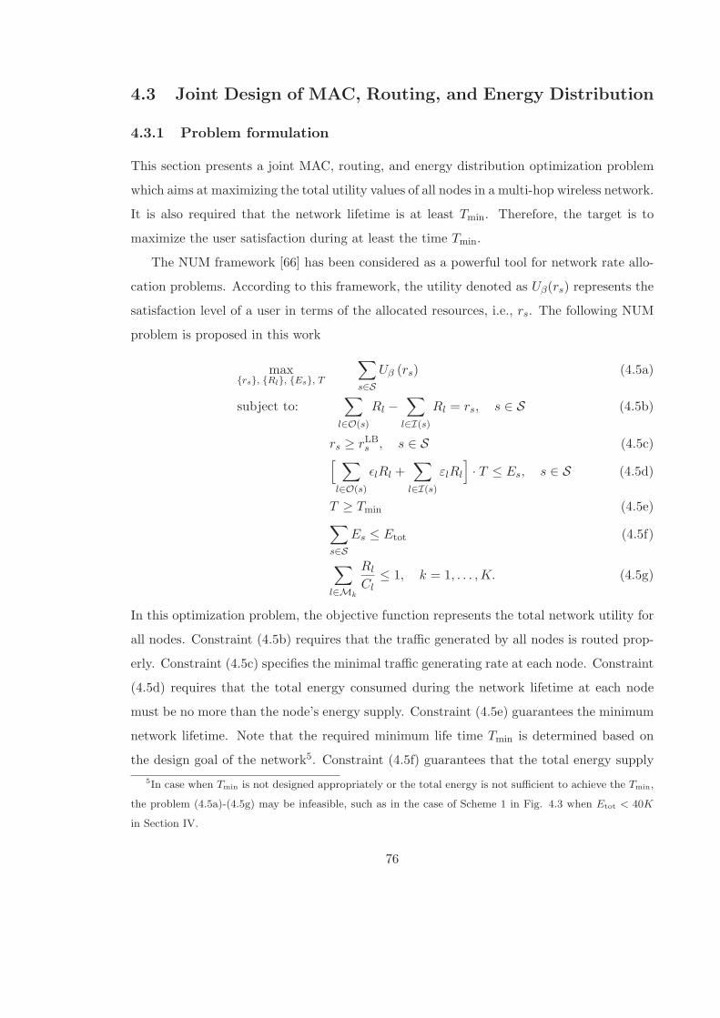
4.3 Joint Design of MAC, Routing, and Energy Distribution
4.3.1 Problem formulation
This section presents a joint MAC, routing, and energy distribution optimization problem
which aims at maximizing the total utility values of all nodes in a multi-hop wireless network.
It is also required that the network lifetime is at least Tmin. Therefore, the target is to
maximize the user satisfaction during at least the time Tmin.
The NUM framework [66] has been considered as a powerful tool for network rate allo-
cation problems. According to this framework, the utility denoted as Uβ(rs) represents the
satisfaction level of a user in terms of the allocated resources, i.e., rs. The following NUM
problem is proposed in this work
max{rs}, {Rl}, {Es}, T
∑
s∈S
Uβ (rs) (4.5a)
subject to:∑
l∈O(s)
Rl −∑
l∈I(s)
Rl = rs, s ∈ S (4.5b)
rs ≥ rLBs , s ∈ S (4.5c)
[
∑
l∈O(s)
ǫlRl +∑
l∈I(s)
εlRl
]
· T ≤ Es, s ∈ S (4.5d)
T ≥ Tmin (4.5e)∑
s∈S
Es ≤ Etot (4.5f)
∑
l∈Mk
Rl
Cl≤ 1, k = 1, . . . , K. (4.5g)
In this optimization problem, the objective function represents the total network utility for
all nodes. Constraint (4.5b) requires that the traffic generated by all nodes is routed prop-
erly. Constraint (4.5c) specifies the minimal traffic generating rate at each node. Constraint
(4.5d) requires that the total energy consumed during the network lifetime at each node
must be no more than the node’s energy supply. Constraint (4.5e) guarantees the minimum
network lifetime. Note that the required minimum life time Tmin is determined based on
the design goal of the network5. Constraint (4.5f) guarantees that the total energy supply
5In case when Tmin is not designed appropriately or the total energy is not sufficient to achieve the Tmin,
the problem (4.5a)-(4.5g) may be infeasible, such as in the case of Scheme 1 in Fig. 4.3 when Etot < 40K
in Section IV.
76
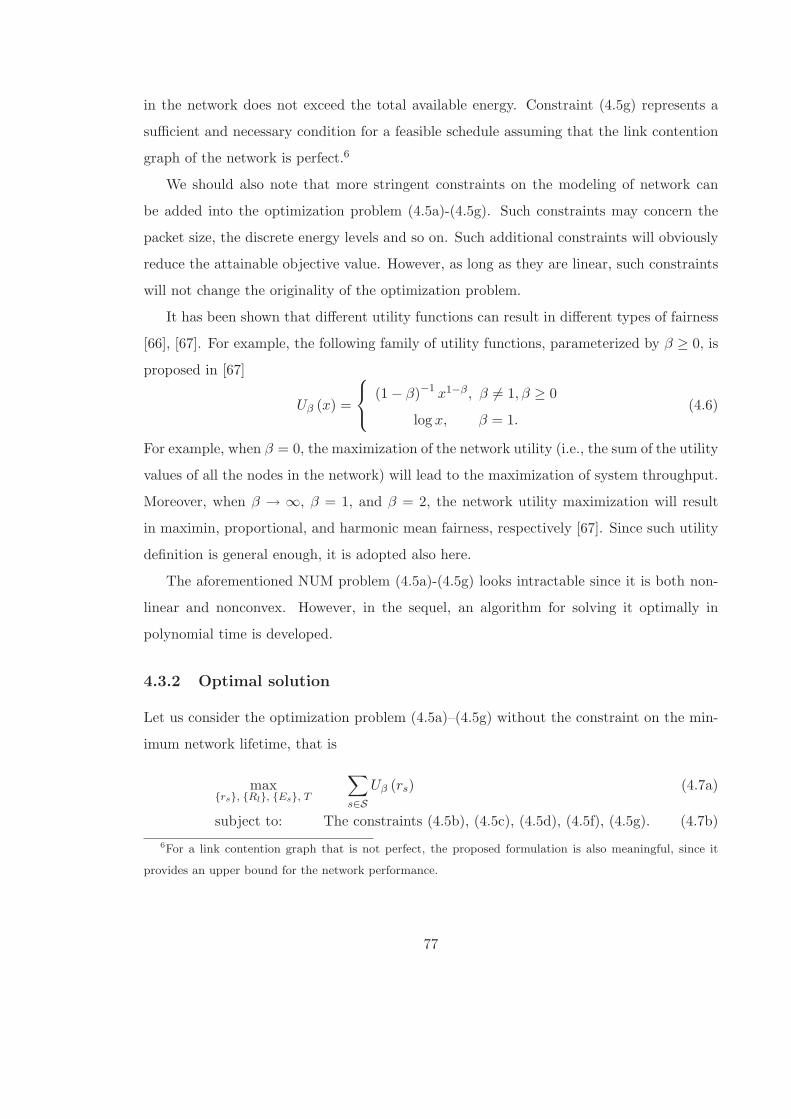
in the network does not exceed the total available energy. Constraint (4.5g) represents a
sufficient and necessary condition for a feasible schedule assuming that the link contention
graph of the network is perfect.6
We should also note that more stringent constraints on the modeling of network can
be added into the optimization problem (4.5a)-(4.5g). Such constraints may concern the
packet size, the discrete energy levels and so on. Such additional constraints will obviously
reduce the attainable objective value. However, as long as they are linear, such constraints
will not change the originality of the optimization problem.
It has been shown that different utility functions can result in different types of fairness
[66], [67]. For example, the following family of utility functions, parameterized by β ≥ 0, is
proposed in [67]
Uβ (x) =
(1 − β)−1 x1−β , β 6= 1, β ≥ 0
log x, β = 1.(4.6)
For example, when β = 0, the maximization of the network utility (i.e., the sum of the utility
values of all the nodes in the network) will lead to the maximization of system throughput.
Moreover, when β → ∞, β = 1, and β = 2, the network utility maximization will result
in maximin, proportional, and harmonic mean fairness, respectively [67]. Since such utility
definition is general enough, it is adopted also here.
The aforementioned NUM problem (4.5a)-(4.5g) looks intractable since it is both non-
linear and nonconvex. However, in the sequel, an algorithm for solving it optimally in
polynomial time is developed.
4.3.2 Optimal solution
Let us consider the optimization problem (4.5a)–(4.5g) without the constraint on the min-
imum network lifetime, that is
max{rs}, {Rl}, {Es}, T
∑
s∈S
Uβ (rs) (4.7a)
subject to: The constraints (4.5b), (4.5c), (4.5d), (4.5f), (4.5g). (4.7b)
6For a link contention graph that is not perfect, the proposed formulation is also meaningful, since it
provides an upper bound for the network performance.
77
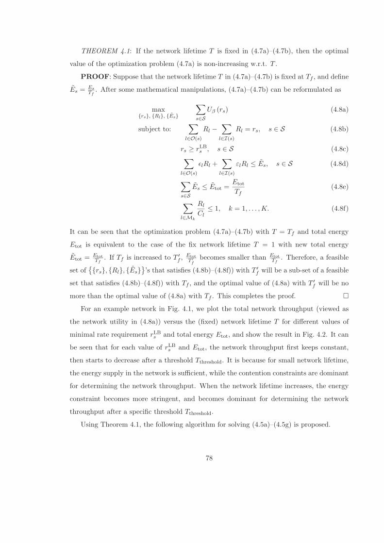
THEOREM 4.1: If the network lifetime T is fixed in (4.7a)–(4.7b), then the optimal
value of the optimization problem (4.7a) is non-increasing w.r.t. T .
PROOF: Suppose that the network lifetime T in (4.7a)–(4.7b) is fixed at Tf , and define
Es = Es
Tf. After some mathematical manipulations, (4.7a)–(4.7b) can be reformulated as
max{rs}, {Rl}, {Es}
∑
s∈S
Uβ (rs) (4.8a)
subject to:∑
l∈O(s)
Rl −∑
l∈I(s)
Rl = rs, s ∈ S (4.8b)
rs ≥ rLBs , s ∈ S (4.8c)
∑
l∈O(s)
ǫlRl +∑
l∈I(s)
εlRl ≤ Es, s ∈ S (4.8d)
∑
s∈S
Es ≤ Etot =Etot
Tf(4.8e)
∑
l∈Mk
Rl
Cl≤ 1, k = 1, . . . , K. (4.8f)
It can be seen that the optimization problem (4.7a)–(4.7b) with T = Tf and total energy
Etot is equivalent to the case of the fix network lifetime T = 1 with new total energy
Etot = EtotTf
. If Tf is increased to T ′f , Etot
T ′
f
becomes smaller than EtotTf
. Therefore, a feasible
set of{
{rs}, {Rl}, {Es}}
’s that satisfies (4.8b)–(4.8f)) with T ′f will be a sub-set of a feasible
set that satisfies (4.8b)–(4.8f)) with Tf , and the optimal value of (4.8a) with T ′f will be no
more than the optimal value of (4.8a) with Tf . This completes the proof. �
For an example network in Fig. 4.1, we plot the total network throughput (viewed as
the network utility in (4.8a)) versus the (fixed) network lifetime T for different values of
minimal rate requirement rLBs and total energy Etot, and show the result in Fig. 4.2. It can
be seen that for each value of rLBs and Etot, the network throughput first keeps constant,
then starts to decrease after a threshold Tthreshold. It is because for small network lifetime,
the energy supply in the network is sufficient, while the contention constraints are dominant
for determining the network throughput. When the network lifetime increases, the energy
constraint becomes more stringent, and becomes dominant for determining the network
throughput after a specific threshold Tthreshold.
Using Theorem 4.1, the following algorithm for solving (4.5a)–(4.5g) is proposed.
78
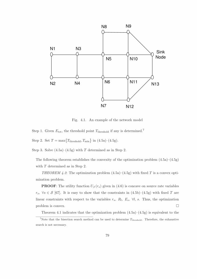
N1Sink
Node
N3
N8 N9
N10N5
N6 N11N13
N12N7
N4N2
Fig. 4.1. An example of the network model
Step 1. Given Etot, the threshold point Tthreshold if any is determined.7
Step 2. Set T = max{
Tthreshold, Tmin
}
in (4.5a)–(4.5g).
Step 3. Solve (4.5a)–(4.5g) with T determined as in Step 2.
The following theorem establishes the convexity of the optimization problem (4.5a)–(4.5g)
with T determined as in Step 2.
THEOREM 4.2: The optimization problem (4.5a)–(4.5g) with fixed T is a convex opti-
mization problem.
PROOF: The utility function Uβ (rs) given in (4.6) is concave on source rate variables
rs, ∀s ∈ S [67]. It is easy to show that the constraints in (4.5b)–(4.5g) with fixed T are
linear constraints with respect to the variables rs, Rl, Es, ∀l, s. Thus, the optimization
problem is convex. �
Theorem 4.1 indicates that the optimization problem (4.5a)–(4.5g) is equivalent to the
7Note that the bisection search method can be used to determine Tthreshold. Therefore, the exhaustive
search is not necessary.
79
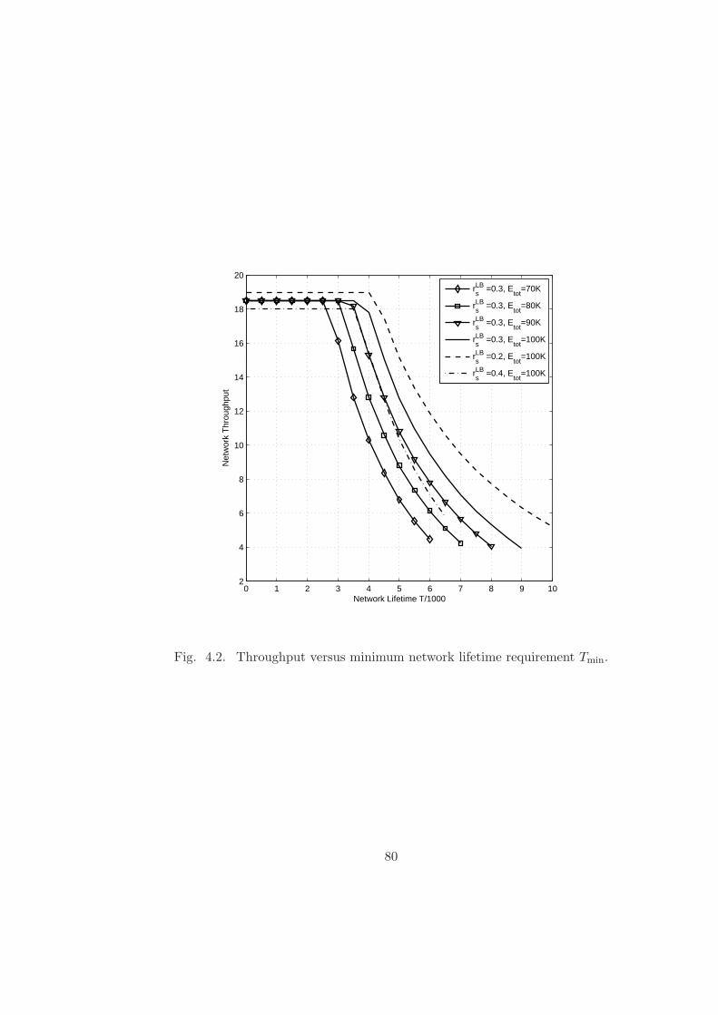
0 1 2 3 4 5 6 7 8 9 102
4
6
8
10
12
14
16
18
20
Network Lifetime T/1000
Net
wor
k T
hrou
ghpu
t
rsLB =0.3, E
tot=70K
rsLB =0.3, E
tot=80K
rsLB =0.3, E
tot=90K
rsLB =0.3, E
tot=100K
rsLB =0.2, E
tot=100K
rsLB =0.4, E
tot=100K
Fig. 4.2. Throughput versus minimum network lifetime requirement Tmin.
80
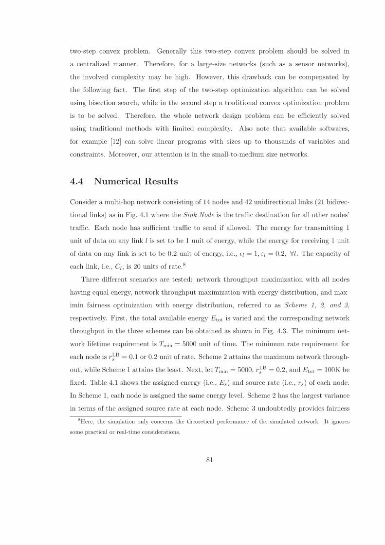
two-step convex problem. Generally this two-step convex problem should be solved in
a centralized manner. Therefore, for a large-size networks (such as a sensor networks),
the involved complexity may be high. However, this drawback can be compensated by
the following fact. The first step of the two-step optimization algorithm can be solved
using bisection search, while in the second step a traditional convex optimization problem
is to be solved. Therefore, the whole network design problem can be efficiently solved
using traditional methods with limited complexity. Also note that available softwares,
for example [12] can solve linear programs with sizes up to thousands of variables and
constraints. Moreover, our attention is in the small-to-medium size networks.
4.4 Numerical Results
Consider a multi-hop network consisting of 14 nodes and 42 unidirectional links (21 bidirec-
tional links) as in Fig. 4.1 where the Sink Node is the traffic destination for all other nodes’
traffic. Each node has sufficient traffic to send if allowed. The energy for transmitting 1
unit of data on any link l is set to be 1 unit of energy, while the energy for receiving 1 unit
of data on any link is set to be 0.2 unit of energy, i.e., ǫl = 1, εl = 0.2, ∀l. The capacity of
each link, i.e., Cl, is 20 units of rate.8
Three different scenarios are tested: network throughput maximization with all nodes
having equal energy, network throughput maximization with energy distribution, and max-
imin fairness optimization with energy distribution, referred to as Scheme 1, 2, and 3,
respectively. First, the total available energy Etot is varied and the corresponding network
throughput in the three schemes can be obtained as shown in Fig. 4.3. The minimum net-
work lifetime requirement is Tmin = 5000 unit of time. The minimum rate requirement for
each node is rLBs = 0.1 or 0.2 unit of rate. Scheme 2 attains the maximum network through-
out, while Scheme 1 attains the least. Next, let Tmin = 5000, rLBs = 0.2, and Etot = 100K be
fixed. Table 4.1 shows the assigned energy (i.e., Es) and source rate (i.e., rs) of each node.
In Scheme 1, each node is assigned the same energy level. Scheme 2 has the largest variance
in terms of the assigned source rate at each node. Scheme 3 undoubtedly provides fairness
8Here, the simulation only concerns the theoretical performance of the simulated network. It ignores
some practical or real-time considerations.
81
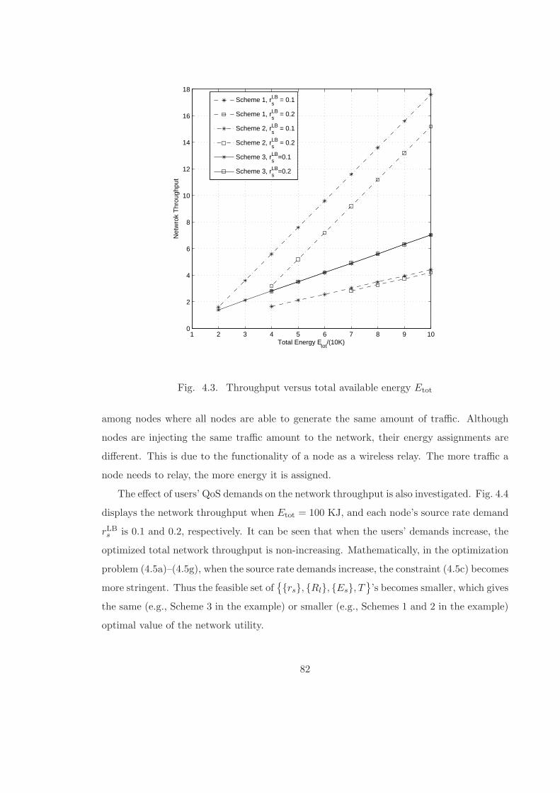
1 2 3 4 5 6 7 8 9 100
2
4
6
8
10
12
14
16
18
Total Energy Etot
/(10K)
Net
wro
k T
hrou
ghpu
t
Scheme 1, r
sLB = 0.1
Scheme 1, rsLB = 0.2
Scheme 2, rsLB = 0.1
Scheme 2, rsLB = 0.2
Scheme 3, rsLB=0.1
Scheme 3, rsLB=0.2
Fig. 4.3. Throughput versus total available energy Etot
among nodes where all nodes are able to generate the same amount of traffic. Although
nodes are injecting the same traffic amount to the network, their energy assignments are
different. This is due to the functionality of a node as a wireless relay. The more traffic a
node needs to relay, the more energy it is assigned.
The effect of users’ QoS demands on the network throughput is also investigated. Fig. 4.4
displays the network throughput when Etot = 100 KJ, and each node’s source rate demand
rLBs is 0.1 and 0.2, respectively. It can be seen that when the users’ demands increase, the
optimized total network throughput is non-increasing. Mathematically, in the optimization
problem (4.5a)–(4.5g), when the source rate demands increase, the constraint (4.5c) becomes
more stringent. Thus the feasible set of{
{rs}, {Rl}, {Es}, T}
’s becomes smaller, which gives
the same (e.g., Scheme 3 in the example) or smaller (e.g., Schemes 1 and 2 in the example)
optimal value of the network utility.
82
0 1 2 3 4 5 6 7 8 9 102
4
6
8
10
12
14
16
18
20
Network Lifetime Tmin
/1000
Net
wor
k T
hrou
ghpu
t
Scheme 1, rsLB = 0.1
Scheme 1, rsLB = 0.2
Scheme 2, rsLB = 0.1
Scheme 2, rsLB = 0.2
Scheme 3, rsLB = 0.1
Scheme 3, rsLB = 0.2
Fig. 4.4. Network throughput versus network lifetime requirement Tmin, Etot = 100 KJ
TABLE 4.1
Assigned energy and source rate at each node when Tmin = 5000, rLBs = 0.2 and
Etot = 100K
Node ID N1 N2 N3 N4 N5 N6 N7 N8 N9 N10 N11 N12 N13
Scheme 1 7.7 7.7 7.7 7.7 7.7 7.7 7.7 7.7 7.7 7.7 7.7 7.7 7.7
Energy Scheme 2 1.4 1.0 3.2 1.8 5.3 2.4 1.0 1.0 23.9 28.2 2.8 2.2 25.9
Scheme 3 3.6 2.7 8.1 5.0 13.3 7.1 2.7 2.7 6.0 23.2 8.3 6.0 11.4
Scheme 1 0.2 0.2 0.2 0.2 0.2 0.2 0.2 0.2 0.9 0.7 0.2 0.2 0.7
Rate Scheme 2 0.2 0.2 0.2 0.2 0.2 0.2 0.2 0.2 4.5 4.3 0.2 0.2 4.4
Scheme 3 0.5 0.5 0.5 0.5 0.5 0.5 0.5 0.5 0.5 0.5 0.5 0.5 0.5
83
4.5 Further Discussions
In the NUM formulation in Section 4.3, the objective is to maximize the user satisfaction,
i.e., network utility, within the minimum required network lifetime. An alternative for-
mulation is to maximize the network utility within the achievable network lifetime, while
guaranteeing that the achievable life time is, at least, as long as the minimum required
network lifetime. For this case, the energy supply at each node (i.e., Es) is fixed, and have
the following NUM problem:
max{rs}, {Rl}, T
T ·∑
s∈S
Uβ (rs) (4.9a)
subject to:∑
l∈O(s)
Rl −∑
l∈I(s)
Rl = rs, s ∈ S (4.9b)
rs ≥ rLBs , s ∈ S (4.9c)
[
∑
l∈O(s)
ǫlRl +∑
l∈I(s)
εlRl
]
· T ≤ Es, s ∈ S (4.9d)
T ≥ Tmin (4.9e)∑
l∈Mk
Rl
Cl≤ 1, k = 1, . . . , K. (4.9f)
THEOREM 4.3: The optimization problem (4.9a)–(4.9f) is quasi-convex.
PROOF: Introducing a new variable B = 1/T , the problem (4.9a)–(4.9f) can be equiv-
alently rewritten as
min{rs}, {Rl}, B
− 1
B·∑
s∈S
Uβ (rs) (4.10a)
subject to:∑
l∈O(s)
ǫlRl +∑
l∈I(s)
εlRl ≤ BEs, s ∈ S (4.10b)
B ≤ 1/Tmin (4.10c)
The constraints (4.9b), (4.9c), (4.9f). (4.10d)
The constraints (4.10b)–(4.10d) in the above problem are linear on variables {rs}, {Rl}and B. In order to prove that the objective function (4.10a) is quasi-convex, consider the
84
following sub-level set
N =
{
{rs}, {Rl}, B∣
∣
∣− 1
B·∑
s∈S
Uβ (rs) ≤ α, α ∈ R}
=
{
{rs}, {Rl}, B∣
∣
∣−∑
s∈S
Uβ (rs) − α · B ≤ 0
}
where α is a constant. Since∑
s∈S Uβ (rs) is concave, −∑s∈S Uβ (rs) is convex. And
α · B is linear on B. Therefore, the set N is convex, and the objective function (4.10a) is
quasi-convex [56]. This completes the proof. �
Note that the problem (4.10a)–(4.10d) can be efficiently solved by traditional methods
such as interior-point methods [56].
4.6 Conclusions
Achieving end-to-end QoS guarantee in multi-hop wireless networks requires a cross-layer
design approach. In this chapter, the joint design of MAC, routing, and energy distribution
in a multi-hop network is formulated as NUM optimization problem. The method for
solving the nonconvex and nonlinear NUM optimization problem optimally is developed. It
is also show that the problem of maximizing sum utility within achievable network lifetime
is quasi-convex. This research should provide insights to the development and deployment
of multi-hop wireless networks, such as wireless sensor networks, mobile ad hoc network,
and wireless mesh networks.
85
Chapter 5
Conclusions and Future Work
THIS THESIS HAS CONSIDERED A NUMBER OF resource allocation problems
for various wireless networks using convex optimization. While the first problem
studied the spectrum sharing in cognitive wireless networks using beamforming techniques,
the second problem investigated the power allocation issue, with and without admission
control, in wireless multi-user relay networks. A cross-layer design problem in multi-hop
wireless networks to maximize the total utility of all users was also studied. Details for each
chapter is summarized as follows.
5.1 Conclusions
Chapter 1 has provided the motivation of the thesis, brief overview of convex optimization
theory on which the results of this thesis are based on, and the outline of the thesis.
Chapter 2 has proposed several problem formulations and solution approaches for multi-
cast beamforming for secondary wireless networks. For such purposes, the thesis considered
practical design scenarios with different criteria involving the interference level at the pri-
mary receivers, the received SNRs of the secondary users and the transmit power. By
exploiting the available CSI via transmit optimization, the network of secondary users is
able to co-exist and exchange information between its users simultaneously with the net-
work of primary users. Although the proposed designs are nonconvex and NP-hard, a
convex relaxation approach coupled with suitable randomization post-processing can pro-
86
vide approximate solutions at a moderate computational cost that is strictly bounded by a
low-order polynomial.
Chapter 3 has focused on the optimal power allocation schemes for multi-user wireless
AF relay networks. Power allocation is done at both the relays and the mobile users.
Specifically, optimal power allocation schemes to i) maximize the minimum end-to-end
SNR among all users; ii) minimize the total transmit power of all sources; iii) maximize the
system throughput were derived. It has been shown that the corresponding optimization
problems can be formulated as GP problems. Therefore, optimal power allocation can
be obtained efficiently even for large-scale networks using convex optimization techniques.
Although GP is nonconvex, it allows for an equivalent convex reformulation which provides
an efficient method for obtaining optimal solution. Moreover, since it may not be possible
to serve every user at its desired QoS demand due to limited power resource, this thesis
have proposed a joint admission control and power allocation algorithm which aimed at first
maximizing the number of users that can be served and then minimizing the transmit power.
Although the original problem is nonconvex and combinatorially hard, a highly efficient GP
heuristic-based algorithm which has running time much smaller than that of the original
optimization problem was developed. This makes the proposed approach attractive for
practical implementation.
Chapter 4 has proposed a joint design of MAC, routing, and energy distribution in a
multi-hop network. The problem has been formulated as NUM optimization problem. The
method for solving the nonconvex and nonlinear NUM optimization problem optimally is
developed. It was also shown that the problem of maximizing sum utility within achievable
network lifetime is quasi-convex. This research should provide insights to the development
and deployment of multi-hop wireless networks, such as wireless sensor networks, mobile ad
hoc network, and wireless mesh networks.
5.2 Future Work
To extend the obtained results, several lines for future research have been recognized.
Regarding the multicast beamforming problem in Chapter 2, it has been assumed that
the design center has perfect channel knowledge from the base station (access point) to both
87
secondary and primary users. However, perfect CSI may not be available in the considered
scenarios. This is because in practice, there is some estimation error in the channel gains
(because of noisy measurements and/or channel variations over time). Therefore, it is
interesting to extend the results which were initially obtained for the case of perfect CSI, to
account for imperfect CSI. Actually, some preliminary results when imperfect CSI is present
have been published [68]. However, the effects of imperfect CSI need to be investigated more
thoroughly. Moreover, broadcasting has also been assumed. This assumption may not be
suitable for some applications where different information needs to be sent to different users.
Semidefinite programming is still a useful tool in this case. However, it is interesting to
investigate the performance of such networks. Another interesting issue is regarding the
admission control problem in such multicast network. Due to limited resources, not all
(secondary) users can always be served at their desirable QoS requirements. Therefore,
some sort of admission control should be carried out and it is interesting to study efficient
admission control algorithms in such cases.
In Chapter 3, the power allocation process is carried out in a centralized manner. In
such context, a central unit (CU) is necessary to coordinate the power allocation at the
sources and at the relays. Moreover, the CU should have channel knowledge for all the
transmission links. This is sometimes impractical due to high complexity, especially for
large-scale networks. Therefore, it is challenging to investigate whether distributed power
allocation via GP is possible. In networks which implement distributed power control,
only local channel information is required for each user. Power allocation is updated by
exchanging control messages between participating relays and users. Therefore, it is scalable
for networks with large sizes. Note that distributed power allocation has been studied
intensively in cellular networks, for example see [2]. Moreover, each source is assumed to
be assisted by one relay which makes it easy to utilize GP. In practice, information from
a source to destination can be forwarded by several relays. It is worth studying efficient
power allocation techniques in this scenario.
Chapter 4 has discussed the cross-layer design in wireless networks to maximize the total
utility of all users. What makes convex programming applicable is the assumption that
utility functions are convex. However, nonconcave utility functions are shown to be more
appropriate in some particular scenarios. In this case, convex programming is unsuitable
88

and global nonconvex programming is necessary. Therefore, it is desirable to look at cross-
layer design problems with nonconvex utility functions.
89
References
[1] G. J. Foschini, and Z. Miljanic, “A simple distributed autonomous power control al-
gorithm and its convergence,” IEEE Trans. Veh. Technol., vol. 42, pp. 641–646, Nov.
1993.
[2] R. D. Yates, “A framework for uplink power control in cellular radio systems,” IEEE
Journal Selected Areas in Communications, vol. 13, pp. 1341–1347, Sept. 1995.
[3] M. Chiang, C. W. Tan, D. Palomar, D. O’Neill, and D. Julian, “Power control by
geometric programming,” IEEE Trans. Wireless Commun., vol. 6, pp. 2640–2651, July
2007.
[4] L. Georgiadis, M. J. Neely, and L. Tassiulas, “Resource allocation and cross-Layer con-
trol in wireless networks,” Foundations and Trends in Networking, vol. 1, pp. 1–144,
2006.
[5] L. B. Le, and E. Hossain, “Multihop cellular networks: Potential gains, research chal-
lenges, and a resource allocation framework,” IEEE Communications Magazine, vol. 45,
pp. 66–73, Sept. 2007.
[6] FCC Spectrum Policy Task Force, “FCC report of the spectrum efficiency working
group,” FCC Technical Report, 2002.
[7] Q. Zhao, and B. M. Sadler, “A survey of dynamic spectrum access,” IEEE Signal Pro-
cessing Magazine, vol. 24, pp. 79–89, May 2007.
[8] J. N. Laneman, D. N. C. Tse, and G. W. Wornell, “Cooperative diversity in wireless
networks: Efficient protocols and outage behavior,” IEEE Trans. Inform. Theory, vol.
50, pp. 3062–3080, Dec. 2004.
90
[9] M. O. Hasna, and M. S. Alouini, “End-to-end performance of transmission systems
with relays over Rayleigh fading channels,” IEEE Trans. Wireless Commun., vol. 2, pp.
1126–1131, Nov. 2003.
[10] X. Lin, N. Shroff, and R. Srikant, “A tutorial on cross-layer optimization in wireless
networks,” IEEE Journal on Selected Areas in Communications, vol. 24, pp. 1452–1463,
Aug. 2006.
[11] M. L. Sichitiu and R. Dutta, “On the lifetime of large wireless sensor networks with
multiple battery levels,” Ad Hoc & Sensor Wireless Networks, to be published.
[12] M. Grant, and S. Boyd, CVX: Matlab software for disciplined convex programming
(web page and software), http://stanford.edu/∼boyd/cvx, February 2008.
[13] J. F. Sturm, “Using SeDuMi 1.02, a MATLAB toolbox for optimization over symmetric
cones,” Optimization Mathematical Software, vol. 11-12, pp. 625–653, Aug. 1999.
[14] J. H. Chang, and L. Tassiulas, “Energy conserving routing in wireless ad-hoc networks,”
in Proc. IEEE INFOCOM, pp. 21–31, Tel-Aviv, Israel, Mar. 2000.
[15] Z. Q. Luo, and W. Yu, “An introduction to convex optimization for communications
and signal processing,” IEEE Journal on Selected Areas in Commun., Special Issue on
Nonlinear Optimization for Communication Systems, vol. 24, pp. 1426–1438, Aug. 2006.
[16] D. P. Palomar, A. Pascual-Iserte, J. M. Cioffi, and M. A. Lagunas, “Convex Opti-
mization Theory Applied to Joint Transmitter-Receiver Design in MIMO Channels” in
Space-Time Processing for MIMO Communications, Chapter 8, pp. 269–318, A. B. Ger-
shman and N. Sidiropoulos, Editors, John Wiley & Sons, April 2005.
[17] S. Boyd, and L. Vandenberghe, Convex Optimization, Cambridge University Press,
2004.
[18] L. Vandenberghe and S. Boyd, “Semidefinite programming,” SIAM Rev., vol. 38, pp.
49–95, Mar. 1996.
[19] Q. Zhao, L. Tong, A. Swami, and Y. Chen, “Decentralized cognitive MAC for oppor-
tunistic spectrum access in ad hoc networks: A POMDP framework,” IEEE J. Select.
91
Areas Commun.: Special Issue on Adaptive, Spectrum Agile and Cognitive Wireless
Networks, vol. 25, pp. 589–600, Apr. 2007.
[20] H. Zheng, and C. Peng, “Collaborative and fairness in opportunistic spectrum access,”
in Proc. IEEE Int. Conf. Commun. (ICC), Korea, May 2005, pp. 3132–3136.
[21] S. Sankaranarayanan, P. Papadimitratos, A. Mishra, “A bandwidth sharing approach
to improve licensed spectrum utilization,” IEEE Communications Magazine, vol. 43,
pp. S10-S14, Dec. 2005.
[22] N. Nie, and C. Comaniciu, “Adaptive channel allocation spectrum etiquette for cogni-
tive radio networks,” in Proc. IEEE New Frontiers in Dynamic Spectrum Access Net-
works (DySPAN), Maryland, USA, Nov. 2005, pp. 269–278.
[23] M. Maskery, V. Krishnamurthy, Q. Zhao, Game Theoretic Learning and Pricing for
Dynamic Spectrum Access in Cognitive Radio, in Cognitive Wireless Communications
Networks, Springer Verlag, Editors: V. Bhargava and E. Hossain, 2007.
[24] M. Maskery, V. Krishnamurthy, and Q. Zhao, “Decentralized dynamic spectrum access
for cognitive radios: Cooperative design of a non-cooperative game”, submitted to IEEE
Trans. on Communs., Mar. 2007.
[25] M. Vu, N. Devroye, M. Sharif, and V. Tarokh, “Scaling laws of cognitive networks,”
in Proc. Int. Conf. Cognitive Radio Oriented Wireless Networks and Communications,
Orlando, Aug. 2007.
[26] T. Hoang, and P. Nguyen-Thi, “A robust algorithm for quadratic optimization under
quadratic constraints,” Journal Global Optimization, vol. 37, pp. 557–569, Apr. 2007.
[27] F. Rashid-Farrokhi, K. J. R. Liu, and L. Tassiulas, “Transmit beamforming and power
control for cellular wireless systems,” IEEE J. Select. Areas Commun., vol. 16, pp.
1437–1450, Oct. 1998.
[28] M. Bengtsson, and B. Ottersten, “Optimal and suboptimal transmit beamforming,”
ch. 18 in Handbook of Antennas in Wireless Communications, L. C. Godara, Ed., CRC
Press, Aug. 2001.
92
[29] N. D. Sidiropoulos, T. N. Davidson, and Z. Q. Luo, “Transmit beamforming for
physical-layer multicasting,” IEEE Trans. Signal Processing, vol. 54, pp. 2239–2251,
June 2006.
[30] S. A. Vorobyov, A. B. Gershman, and Z. Q. Luo, “Robust adaptive beamforming using
worst-case performance optimization: A solution to the signal mismatch problem,” IEEE
Trans. Signal Processing, vol. 51, pp. 313–324, Feb. 2003.
[31] S. Haykin, “Cognitive radio: brain-empowered wireless communications,” IEEE J.
Select. Areas Commun., vol. 23, pp. 201220, Feb. 2005.
[32] M. H. Islam, Y. C. Liang, and A. T. Hoang, “Joint beamforming and power control
in the downlink of cognitive radio networks,” in Proc. IEEE Wireless Commun. and
Networking Conf. (WCNC), HongKong, Mar. 2007, pp. 21–26.
[33] H. Boche, and M. Schubert, “A general duality theory for uplink and downlink beam-
forming,” in Proc. IEEE Veh. Tech. Conf. (VTC) Fall, Vancouver, Canada, Sept. 2002,
pp. 87–91.
[34] L. B. Le, and E. Hossain, “QoS-aware spectrum sharing in cognitive wireless networks,”
in Proc. IEEE Global Telecommunications Conference (GLOBECOM), Washington DC,
USA, Nov. 2007, pp. 3563–3567.
[35] Z. Q. Luo, N. D. Sidiropoulos, P. Tseng, and S. Zhang, “Approximation bounds for
quadratic optimization with homogeneous quadratic constraints,” SIAM Journal Opti-
mization, vol. 18, pp. 1–28, 2007.
[36] T. Jiang, N. D. Sidiropoulos, and J. M. F. ten Berge, “Almost sure identifiability of
multi-dimensional harmonic retrieval,” IEEE Trans. Signal Processing, vol. 49, no. 9,
pp. 1849-1859, Sep. 2001.
[37] A. Wiesel, Y. C. Eldar, and S. Shamai, “Semidefinite relaxation for detection of 16-
QAM signaling in MIMO channels,” IEEE Signal Process. Lett., vol. 12, pp. 653–656,
Sept. 2005.
[38] A. Ben Tal, and A. Nemirovski, “Lectures on modern convex optimization,” MPS-
SIAM Series on Optimization, 2001.
93
[39] A. Papoulis, Probability, Random Variables, and Stochastic Processes, 3rd ed. New
York: McGraw-Hill, 1991.
[40] W. K. Ma, T. N. Davidson, K. M. Wong, Z. Q. Luo, and P.-C. Ching, “Quasi-ML mul-
tiuser detection using semi-definite relaxation with application to synchronous CDMA,”
IEEE Trans. Signal Processing, vol. 50, pp. 912–922, Apr. 2002.
[41] S. Zhang, “Quadratic maximization and semidefinite relaxation,” Mathematical Pro-
gramming, vol. 87, pp. 453–465, May 2000.
[42] P. Tseng, “Further results on approximating nonconvex quadratic optimization by
semidefinite programming relaxation,” SIAM Journal Optimization, vol. 14, pp. 268–
283, Jul. 2003.
[43] H. Wolkowicz, Relaxations of Q2P, in Handbook of Semidefinite Programming: Theory,
Algorithms, and Applications, chapter 13.4, H. Wolkowicz, R. Saigal, and L. Vanden-
berghe, Eds. Norwell, MA: Kluwer, 2000.
[44] P. A. Anghel, and M. Kaveh, “Exact symbol error probability of a cooperative network
in a Rayleigh-fading environment,” IEEE Trans. Wireless Commun., vol. 3, pp. 1416–
1421, Sept. 2004.
[45] S. Ikki, and M. H. Ahmed, “Performance analysis of cooperative diversity wireless
networks over Nakagami-m fading channel,” IEEE Commun. Letters, vol. 11, pp. 334–
336, Jul. 2007.
[46] N. C. Beaulieu, and J. Hu, “A closed-form expression for the outage probability of
decode-and-forward relaying in dissimilar Rayleigh fading channels,” IEEE Commun.
Letters, vol. 10, pp. 813–815, Dec. 2006.
[47] Y. Li, B. Vucetic, Z. Zhou, and M. Dohler, “Distributed adaptive power allocation for
wireless relay networks,” IEEE Trans. Wireless Commun., vol. 6, pp. 948–958, Mar.
2007.
[48] M. Chen, S. Serbetli, and A. Yener, “Distributed power allocation strategies for parallel
relay networks,” IEEE Trans. Wireless Commun., vol. 7, pp. 552–561, Feb. 2008.
94
[49] X. Deng, and A. M. Haimovich, “Power allocation for cooperative relaying in wireless
networks,” IEEE Commun. Letters, vol. 9, pp. 994–996, Nov. 2005.
[50] A. H. Madsen, and J. Zhang, “Capacity bounds and power allocation for wireless relay
channels,” IEEE Trans. Inform. Theory, vol. 51, pp. 2020–2040, June 2005.
[51] Y. Liang, and V. Veeravalli, “Gaussian orthogonal relay channel: optimal resource
allocation and capacity,” IEEE Trans. Inform. Theory, vol. 51, pp. 3284–3289, Sept.
2005.
[52] Y. Zhao, R. S. Adve, and T. J. Lim, “Improving amplify-and-forward relay networks:
optimal power allocation versus selection,” IEEE Trans. on Wireless Commun., vol. 6,
pp. 3114–3123, Aug. 2007.
[53] L. B. Le, and E. Hossain, “Cross-layer optimization frameworks for multihop wireless
networks using cooperative diversity,” IEEE Trans. Wireless Commun., to appear.
[54] Truman Chiu-Yam Ng, and Wei Yu, “Joint optimization of relay strategies and re-
source allocations in a cooperative cellular network,” IEEE Journal on Selected Areas
in Commun., vol. 25, pp. 328–339, Feb. 2007.
[55] Z. Zhang, W. Zhang, and C. Tellambura, “Improved OFDMA uplink frequency off-
set estimation via cooperative relaying: AF or D&F ?,” in Proc. IEEE Inter. Conf.
Commun. (ICC), Beijjing, China, May 2008.
[56] D. Julian, M. Chiang, D. O’Neill, and S. P. Boyd, “QoS and fairness constrained convex
optimization of resource allocation for wireless cellular and ad hoc networks,” in Proc.
IEEE INFOCOM, New York, NY, Jun. 2002, pp. 477–486.
[57] A. Goldsmith, Wireless Communications, Cambridge University Press, 2004.
[58] C. C. Wu, and D. P. Bertsekas, “Admission control for wireless networks,” IEEE Trans.
on Vehicular Tech., to appear.
[59] E. Matskani, N. D. Sidiropoulos, Z. Q. Luo, and L. Tassiulas, “Joint multiuser downlink
beamforming and admission control: A semidefinite relaxation approach,” in Proc. IEEE
95
Inter. Conf. Accous. Speech and Sig. Proc. (ICASSP), Hawaii, USA, Apr. 2007, pp. 585–
588.
[60] H. T. Cheng, H. Jiang, and W. Zhuang, “Distributed medium access control for wireless
mesh networks,” Wireless Communications and Mobile Computing, vol. 6, pp. 845–864,
Sept. 2006.
[61] X. Shen, W. Zhuang, H. Jiang, and J. Cai, “Medium access control in ultra-wideband
wireless networks,” IEEE Trans. Veh. Technol., vol. 54, pp. 1663–1677, Sept. 2005.
[62] S. J. Kim, X. Wang, and M. Madihian, “Distributed joint routing and medium access
control for lifetime maximization of wireless sensor networks,” IEEE Trans. Wireless
Commun., vol. 6, pp. 2669–2677, July 2007.
[63] T. Nandagopal, T. E. Kim, X. Gao, and V. Bharghavan, “Achieving MAC layer fairness
in wireless packet networks,” in Proc. Inter. Conf. Mobile Computing and Networking
(MOBICOM), Massachusetts, USA, Aug. 2000, pp. 87–98.
[64] Z. Fang and B. Bensaou, “Fair bandwidth sharing algorithms based on game theory
frameworks for wireless ad-hoc networks,” in Proc. IEEE INFOCOM, HongKong, Mar.
2004, pp. 1284–1295.
[65] L. Chen, S. H. Low, and J. C. Doyle, “Joint congestion control and media access
control design for ad hoc wireless networks,” in Proc. IEEE INFOCOM, Miami, USA,
Mar. 2005, pp. 2212–2222.
[66] F. P. Kelly, A. K. Maulloo, and D. K. H. Tan, “Rate control in communication net-
works: shadow prices, proportional fairness and stability,” Journal Optical Research
Society, vol. 49, pp. 237–252, Mar. 1998..
[67] J. Mo, and J. Walrand, “Fair end-to-end window-based congestion control,”
IEEE/ACM Trans. Networking, vol. 8, pp. 556–567, Oct. 2000.
[68] K. T. Phan, S. A.Vorobyov, N. D. Sidiropoulos, and C. Telambura, “Spectrum sharing
in wireless networks: A QoS-aware secondary multicast approach with worst user per-
formance optimization,” in Proc. IEEE Workshop on Sensor Array and Multi-Channel
Signal Processing (SAM), Darmstadt, Germany, July 2008.
96


