cdma2000 Measurement Application Measurement Guide and...
140
Measurement Guide and Programming Examples N9072A cdma2000 Measurement Application This manual provides documentation for the following X-Series Analyzers: MXA Signal Analyzer N9020A EXA Signal Analyzer N9010A Manufacturing Part Number: N9072-90002 Printed in USA November 2007 © Copyright 2007 Agilent Technologies, Inc.
Transcript of cdma2000 Measurement Application Measurement Guide and...

Measurement Guide and Programming Examples
N9072A cdma2000 Measurement Application
This manual provides documentation for the following X-Series Analyzers:
MXA Signal Analyzer N9020AEXA Signal Analyzer N9010A
Manufacturing Part Number: N9072-90002Printed in USANovember 2007
© Copyright 2007 Agilent Technologies, Inc.

Legal InformationThe information contained in this document is subject to change without notice.
Agilent Technologies makes no warranty of any kind with regard to this material, including but not limited to, the implied warranties of merchantability and fitness for a particular purpose. Agilent Technologies shall not be liable for errors contained herein or for incidental or consequential damages in connection with the furnishing, performance, or use of this material.
Where to Find the Latest Information
Documentation is updated periodically.
• For the latest information about Agilent Technologies Signal Analyzers, including software upgrades and application information, go to:
http://www.agilent.com/find/mxa
http://www.agilent.com/find/exa
Technology Licenses The hardware and/or software described in this document are furnished under a license and may be used or copied only in accordance with the terms of such license.
Restricted Rights LegendIf software is for use in the performance of a U.S. Government prime contract or subcontract, Software is delivered and licensed as “Commercial computer software” as defined in DFAR 252.227-7014 (June 1995), or as a “commercial item” as defined in FAR 2.101(a) or as “Restricted computer software” as defined in FAR 52.227-19 (June 1987) or any equivalent agency regulation or contract clause. Use, duplication or disclosure of Software is subject to Agilent Technologies’ standard commercial license terms, and non-DOD Departments and Agencies of the U.S. Government will receive no greater than Restricted Rights as defined in FAR 52.227-19(c)(1-2) (June 1987). U.S. Government users will receive no greater than Limited Rights as defined in FAR 52.227-14 (June 1987) or DFAR 252.227-7015 (b)(2) (November 1995), as applicable in any technical data.
2

ContentsTable of C
ontents
1. Making cdma2000 MeasurementsSetting Up and Making a Measurement . . . . . . . . . . . . . . . . . . . . . . . . . . . . . . . . . . . . . . . . . . . . . . . . . . . . . 8
Making the Initial Signal Connection . . . . . . . . . . . . . . . . . . . . . . . . . . . . . . . . . . . . . . . . . . . . . . . . . . . . . 8Using Analyzer Mode and Measurement Presets . . . . . . . . . . . . . . . . . . . . . . . . . . . . . . . . . . . . . . . . . . . . 8The 3 Steps to Set Up and Make Measurements. . . . . . . . . . . . . . . . . . . . . . . . . . . . . . . . . . . . . . . . . . . . . 8
2. Channel Power MeasurementsSetting Up and Making a Measurement . . . . . . . . . . . . . . . . . . . . . . . . . . . . . . . . . . . . . . . . . . . . . . . . . . . . 12
Configuring the Measurement System . . . . . . . . . . . . . . . . . . . . . . . . . . . . . . . . . . . . . . . . . . . . . . . . . . . 12Setting the MS (Example) . . . . . . . . . . . . . . . . . . . . . . . . . . . . . . . . . . . . . . . . . . . . . . . . . . . . . . . . . . . . . 12Measurement Procedure . . . . . . . . . . . . . . . . . . . . . . . . . . . . . . . . . . . . . . . . . . . . . . . . . . . . . . . . . . . . . . 13
3. ACP MeasurementsSetting Up and Making a Measurement . . . . . . . . . . . . . . . . . . . . . . . . . . . . . . . . . . . . . . . . . . . . . . . . . . . . 16
Configuring the Measurement System . . . . . . . . . . . . . . . . . . . . . . . . . . . . . . . . . . . . . . . . . . . . . . . . . . . 16Setting the MS (Example) . . . . . . . . . . . . . . . . . . . . . . . . . . . . . . . . . . . . . . . . . . . . . . . . . . . . . . . . . . . . . 16Measurement Procedure . . . . . . . . . . . . . . . . . . . . . . . . . . . . . . . . . . . . . . . . . . . . . . . . . . . . . . . . . . . . . . 17
4. Spectrum Emission Mask MeasurementsSetting Up and Making a Measurement . . . . . . . . . . . . . . . . . . . . . . . . . . . . . . . . . . . . . . . . . . . . . . . . . . . . 22
Configuring the Measurement System . . . . . . . . . . . . . . . . . . . . . . . . . . . . . . . . . . . . . . . . . . . . . . . . . . . 22Setting the MS (Example) . . . . . . . . . . . . . . . . . . . . . . . . . . . . . . . . . . . . . . . . . . . . . . . . . . . . . . . . . . . . . 22Measurement Procedure . . . . . . . . . . . . . . . . . . . . . . . . . . . . . . . . . . . . . . . . . . . . . . . . . . . . . . . . . . . . . . 23Troubleshooting Hints . . . . . . . . . . . . . . . . . . . . . . . . . . . . . . . . . . . . . . . . . . . . . . . . . . . . . . . . . . . . . . . . 24
5. Spurious Emissions MeasurementSetting Up and Making a Measurement . . . . . . . . . . . . . . . . . . . . . . . . . . . . . . . . . . . . . . . . . . . . . . . . . . . . 28
Configuring the Measurement System . . . . . . . . . . . . . . . . . . . . . . . . . . . . . . . . . . . . . . . . . . . . . . . . . . . 28Setting up the MS (Example) . . . . . . . . . . . . . . . . . . . . . . . . . . . . . . . . . . . . . . . . . . . . . . . . . . . . . . . . . . 28Measurement Procedure . . . . . . . . . . . . . . . . . . . . . . . . . . . . . . . . . . . . . . . . . . . . . . . . . . . . . . . . . . . . . . 28Measurement Results . . . . . . . . . . . . . . . . . . . . . . . . . . . . . . . . . . . . . . . . . . . . . . . . . . . . . . . . . . . . . . . . 29
6. Occupied Bandwidth MeasurementsSetting Up and Making a Measurement . . . . . . . . . . . . . . . . . . . . . . . . . . . . . . . . . . . . . . . . . . . . . . . . . . . . 34
Configuring the Measurement System . . . . . . . . . . . . . . . . . . . . . . . . . . . . . . . . . . . . . . . . . . . . . . . . . . . 34Setting the MS (Example) . . . . . . . . . . . . . . . . . . . . . . . . . . . . . . . . . . . . . . . . . . . . . . . . . . . . . . . . . . . . . 34Measurement Procedure . . . . . . . . . . . . . . . . . . . . . . . . . . . . . . . . . . . . . . . . . . . . . . . . . . . . . . . . . . . . . . 35Troubleshooting Hints . . . . . . . . . . . . . . . . . . . . . . . . . . . . . . . . . . . . . . . . . . . . . . . . . . . . . . . . . . . . . . . . 35
7. Code Domain MeasurementsSetting Up and Making a Measurement . . . . . . . . . . . . . . . . . . . . . . . . . . . . . . . . . . . . . . . . . . . . . . . . . . . . 38
cdma2000 Measurement Example (MS). . . . . . . . . . . . . . . . . . . . . . . . . . . . . . . . . . . . . . . . . . . . . . . . . . 38cdma2000 Measurement Example (BTS) . . . . . . . . . . . . . . . . . . . . . . . . . . . . . . . . . . . . . . . . . . . . . . . . . 47Troubleshooting Hints . . . . . . . . . . . . . . . . . . . . . . . . . . . . . . . . . . . . . . . . . . . . . . . . . . . . . . . . . . . . . . . . 52
8. Modulation Accuracy (Composite Rho) MeasurementsSetting Up and Making a Measurement . . . . . . . . . . . . . . . . . . . . . . . . . . . . . . . . . . . . . . . . . . . . . . . . . . . . 56
3
ContentsTa
ble
of C
onte
nts
cdma2000 Measurement Example (MS) . . . . . . . . . . . . . . . . . . . . . . . . . . . . . . . . . . . . . . . . . . . . . . . . . 56cdma2000 Measurement Example (BTS). . . . . . . . . . . . . . . . . . . . . . . . . . . . . . . . . . . . . . . . . . . . . . . . . 61Troubleshooting Hints. . . . . . . . . . . . . . . . . . . . . . . . . . . . . . . . . . . . . . . . . . . . . . . . . . . . . . . . . . . . . . . . 64
9. Power Statistics CCDF MeasurementsSetting Up and Making a Measurement . . . . . . . . . . . . . . . . . . . . . . . . . . . . . . . . . . . . . . . . . . . . . . . . . . . . 66
Configuring the Measurement System . . . . . . . . . . . . . . . . . . . . . . . . . . . . . . . . . . . . . . . . . . . . . . . . . . . 66Setting the MS (Example). . . . . . . . . . . . . . . . . . . . . . . . . . . . . . . . . . . . . . . . . . . . . . . . . . . . . . . . . . . . . 66Measurement Procedure . . . . . . . . . . . . . . . . . . . . . . . . . . . . . . . . . . . . . . . . . . . . . . . . . . . . . . . . . . . . . . 67Troubleshooting Hints. . . . . . . . . . . . . . . . . . . . . . . . . . . . . . . . . . . . . . . . . . . . . . . . . . . . . . . . . . . . . . . . 68
10. QPSK EVM MeasurementsSetting Up and Making a Measurement . . . . . . . . . . . . . . . . . . . . . . . . . . . . . . . . . . . . . . . . . . . . . . . . . . . . 70
Configuring the Measurement System . . . . . . . . . . . . . . . . . . . . . . . . . . . . . . . . . . . . . . . . . . . . . . . . . . . 70Setting the MS . . . . . . . . . . . . . . . . . . . . . . . . . . . . . . . . . . . . . . . . . . . . . . . . . . . . . . . . . . . . . . . . . . . . . 70Measurement Procedure . . . . . . . . . . . . . . . . . . . . . . . . . . . . . . . . . . . . . . . . . . . . . . . . . . . . . . . . . . . . . . 71Troubleshooting Hints. . . . . . . . . . . . . . . . . . . . . . . . . . . . . . . . . . . . . . . . . . . . . . . . . . . . . . . . . . . . . . . . 73
11. Monitor Spectrum MeasurementsSetting Up and Making a Measurement . . . . . . . . . . . . . . . . . . . . . . . . . . . . . . . . . . . . . . . . . . . . . . . . . . . . 76
Configuring the Measurement System . . . . . . . . . . . . . . . . . . . . . . . . . . . . . . . . . . . . . . . . . . . . . . . . . . . 76Setting the MS (Example). . . . . . . . . . . . . . . . . . . . . . . . . . . . . . . . . . . . . . . . . . . . . . . . . . . . . . . . . . . . . 76Measurement Procedure . . . . . . . . . . . . . . . . . . . . . . . . . . . . . . . . . . . . . . . . . . . . . . . . . . . . . . . . . . . . . . 77
12. IQ Waveform (Time Domain) MeasurementsSetting Up and Making Measurements . . . . . . . . . . . . . . . . . . . . . . . . . . . . . . . . . . . . . . . . . . . . . . . . . . . . 80
Configuring the Measurement System . . . . . . . . . . . . . . . . . . . . . . . . . . . . . . . . . . . . . . . . . . . . . . . . . . . 80Setting the MS (Example). . . . . . . . . . . . . . . . . . . . . . . . . . . . . . . . . . . . . . . . . . . . . . . . . . . . . . . . . . . . . 80Measurement Procedure . . . . . . . . . . . . . . . . . . . . . . . . . . . . . . . . . . . . . . . . . . . . . . . . . . . . . . . . . . . . . . 81
13. ConceptsWhat Is the cdma2000 Communication System?. . . . . . . . . . . . . . . . . . . . . . . . . . . . . . . . . . . . . . . . . . . . . 86
Introduction. . . . . . . . . . . . . . . . . . . . . . . . . . . . . . . . . . . . . . . . . . . . . . . . . . . . . . . . . . . . . . . . . . . . . . . . 86Spreading Rate . . . . . . . . . . . . . . . . . . . . . . . . . . . . . . . . . . . . . . . . . . . . . . . . . . . . . . . . . . . . . . . . . . . . . 87Radio Configuration . . . . . . . . . . . . . . . . . . . . . . . . . . . . . . . . . . . . . . . . . . . . . . . . . . . . . . . . . . . . . . . . . 87Forward Link Air Interface. . . . . . . . . . . . . . . . . . . . . . . . . . . . . . . . . . . . . . . . . . . . . . . . . . . . . . . . . . . . 87Reverse link air interface — HPSK . . . . . . . . . . . . . . . . . . . . . . . . . . . . . . . . . . . . . . . . . . . . . . . . . . . . . 89Forward link power control . . . . . . . . . . . . . . . . . . . . . . . . . . . . . . . . . . . . . . . . . . . . . . . . . . . . . . . . . . . 91Differences between cdma2000 and W-CDMA . . . . . . . . . . . . . . . . . . . . . . . . . . . . . . . . . . . . . . . . . . . . 92
Adjacent Channel Power (ACP) Measurement Concepts . . . . . . . . . . . . . . . . . . . . . . . . . . . . . . . . . . . . . . 93Purpose . . . . . . . . . . . . . . . . . . . . . . . . . . . . . . . . . . . . . . . . . . . . . . . . . . . . . . . . . . . . . . . . . . . . . . . . . . . 93Measurement Method . . . . . . . . . . . . . . . . . . . . . . . . . . . . . . . . . . . . . . . . . . . . . . . . . . . . . . . . . . . . . . . . 93
Channel Power Measurement Concepts. . . . . . . . . . . . . . . . . . . . . . . . . . . . . . . . . . . . . . . . . . . . . . . . . . . . 95Purpose . . . . . . . . . . . . . . . . . . . . . . . . . . . . . . . . . . . . . . . . . . . . . . . . . . . . . . . . . . . . . . . . . . . . . . . . . . . 95Measurement Method . . . . . . . . . . . . . . . . . . . . . . . . . . . . . . . . . . . . . . . . . . . . . . . . . . . . . . . . . . . . . . . . 95
Code Domain Measurement Concepts . . . . . . . . . . . . . . . . . . . . . . . . . . . . . . . . . . . . . . . . . . . . . . . . . . . . . 96Purpose . . . . . . . . . . . . . . . . . . . . . . . . . . . . . . . . . . . . . . . . . . . . . . . . . . . . . . . . . . . . . . . . . . . . . . . . . . . 96Measurement Method . . . . . . . . . . . . . . . . . . . . . . . . . . . . . . . . . . . . . . . . . . . . . . . . . . . . . . . . . . . . . . . . 96
4

ContentsTable of C
ontents
Modulation Accuracy (Composite Rho) Measurement Concepts . . . . . . . . . . . . . . . . . . . . . . . . . . . . . . . . 98Purpose . . . . . . . . . . . . . . . . . . . . . . . . . . . . . . . . . . . . . . . . . . . . . . . . . . . . . . . . . . . . . . . . . . . . . . . . . . . 98Measurement Method . . . . . . . . . . . . . . . . . . . . . . . . . . . . . . . . . . . . . . . . . . . . . . . . . . . . . . . . . . . . . . . . 98
Occupied Bandwidth Measurement Concepts . . . . . . . . . . . . . . . . . . . . . . . . . . . . . . . . . . . . . . . . . . . . . . 100Purpose . . . . . . . . . . . . . . . . . . . . . . . . . . . . . . . . . . . . . . . . . . . . . . . . . . . . . . . . . . . . . . . . . . . . . . . . . . 100Measurement Method . . . . . . . . . . . . . . . . . . . . . . . . . . . . . . . . . . . . . . . . . . . . . . . . . . . . . . . . . . . . . . . 100
Power Statistics CCDF Measurement Concepts. . . . . . . . . . . . . . . . . . . . . . . . . . . . . . . . . . . . . . . . . . . . . 101Purpose . . . . . . . . . . . . . . . . . . . . . . . . . . . . . . . . . . . . . . . . . . . . . . . . . . . . . . . . . . . . . . . . . . . . . . . . . . 101Measurement Method . . . . . . . . . . . . . . . . . . . . . . . . . . . . . . . . . . . . . . . . . . . . . . . . . . . . . . . . . . . . . . . 103
QPSK EVM Measurement Concepts . . . . . . . . . . . . . . . . . . . . . . . . . . . . . . . . . . . . . . . . . . . . . . . . . . . . . 104Purpose . . . . . . . . . . . . . . . . . . . . . . . . . . . . . . . . . . . . . . . . . . . . . . . . . . . . . . . . . . . . . . . . . . . . . . . . . . 104Measurement Method . . . . . . . . . . . . . . . . . . . . . . . . . . . . . . . . . . . . . . . . . . . . . . . . . . . . . . . . . . . . . . . 107
Monitor Spectrum Measurement Concepts . . . . . . . . . . . . . . . . . . . . . . . . . . . . . . . . . . . . . . . . . . . . . . . . 108Purpose . . . . . . . . . . . . . . . . . . . . . . . . . . . . . . . . . . . . . . . . . . . . . . . . . . . . . . . . . . . . . . . . . . . . . . . . . . 108Measurement Method . . . . . . . . . . . . . . . . . . . . . . . . . . . . . . . . . . . . . . . . . . . . . . . . . . . . . . . . . . . . . . . 108Troubleshooting Hints . . . . . . . . . . . . . . . . . . . . . . . . . . . . . . . . . . . . . . . . . . . . . . . . . . . . . . . . . . . . . . . 108
Spectrum Emission Mask Measurement Concepts. . . . . . . . . . . . . . . . . . . . . . . . . . . . . . . . . . . . . . . . . . . 109Purpose . . . . . . . . . . . . . . . . . . . . . . . . . . . . . . . . . . . . . . . . . . . . . . . . . . . . . . . . . . . . . . . . . . . . . . . . . . 109Measurement Method . . . . . . . . . . . . . . . . . . . . . . . . . . . . . . . . . . . . . . . . . . . . . . . . . . . . . . . . . . . . . . . 109
Spurious Emissions Measurement Concepts . . . . . . . . . . . . . . . . . . . . . . . . . . . . . . . . . . . . . . . . . . . . . . . 110Purpose . . . . . . . . . . . . . . . . . . . . . . . . . . . . . . . . . . . . . . . . . . . . . . . . . . . . . . . . . . . . . . . . . . . . . . . . . . 110Measurement Method . . . . . . . . . . . . . . . . . . . . . . . . . . . . . . . . . . . . . . . . . . . . . . . . . . . . . . . . . . . . . . . 110
IQ Waveform Measurement Concepts . . . . . . . . . . . . . . . . . . . . . . . . . . . . . . . . . . . . . . . . . . . . . . . . . . . . 111Purpose . . . . . . . . . . . . . . . . . . . . . . . . . . . . . . . . . . . . . . . . . . . . . . . . . . . . . . . . . . . . . . . . . . . . . . . . . . 111Measurement Method . . . . . . . . . . . . . . . . . . . . . . . . . . . . . . . . . . . . . . . . . . . . . . . . . . . . . . . . . . . . . . . 111
Other Sources of Measurement Information . . . . . . . . . . . . . . . . . . . . . . . . . . . . . . . . . . . . . . . . . . . . . . . 112Instrument Updates at www.agilent.com . . . . . . . . . . . . . . . . . . . . . . . . . . . . . . . . . . . . . . . . . . . . . . . . 112
References. . . . . . . . . . . . . . . . . . . . . . . . . . . . . . . . . . . . . . . . . . . . . . . . . . . . . . . . . . . . . . . . . . . . . . . . . . 113
14. Programming ExamplesAvailable Programing Examples. . . . . . . . . . . . . . . . . . . . . . . . . . . . . . . . . . . . . . . . . . . . . . . . . . . . . . . . . 116Programming Fundamentals . . . . . . . . . . . . . . . . . . . . . . . . . . . . . . . . . . . . . . . . . . . . . . . . . . . . . . . . . . . . 119
SCPI Language Basics . . . . . . . . . . . . . . . . . . . . . . . . . . . . . . . . . . . . . . . . . . . . . . . . . . . . . . . . . . . . . . 120Improving Measurement Speed . . . . . . . . . . . . . . . . . . . . . . . . . . . . . . . . . . . . . . . . . . . . . . . . . . . . . . . 127Programming in C Using the VTL . . . . . . . . . . . . . . . . . . . . . . . . . . . . . . . . . . . . . . . . . . . . . . . . . . . . . 131
5

ContentsTa
ble
of C
onte
nts
6
1 Making cdma2000 Measurements
This chapter begins with instructions common to all measurements, then details all the measurements available by pressing the Meas key when the cdma2000 mode is selected. For information specific to individual measurements, see the sections at the page numbers below.
• “Channel Power Measurements” on page 11
• “ACP Measurements” on page 15
• “Spectrum Emission Mask Measurements” on page 21
• “Spurious Emissions Measurement” on page 27
• “Occupied Bandwidth Measurements” on page 33
• “Power Statistics CCDF Measurements” on page 65
• “Code Domain Measurements” on page 37
• “Modulation Accuracy (Composite Rho) Measurements” on page 55
• “QPSK EVM Measurements” on page 69
• “Monitor Spectrum Measurements” on page 75
• “IQ Waveform (Time Domain) Measurements” on page 79
7
Making cdma2000 MeasurementsSetting Up and Making a Measurement
Mak
ing
cdm
a200
0 M
easu
rem
ents
Setting Up and Making a Measurement
Making the Initial Signal Connection
CAUTION Before connecting a signal to the analyzer, make sure the analyzer can safely accept the signal level provided. The signal level limits are marked next to the RF Input connectors on the front panel.
See the Input Key menu for details on selecting input ports and the AMPTD Y Scale menu for details on setting internal attenuation to prevent overloading the analyzer.
Using Analyzer Mode and Measurement Presets
To set your current measurement mode to a known factory default state, press Mode Preset. This initializes the analyzer by returning the mode setup and all of the measurement setups in the mode to the factory default parameters.
To preset the parameters that are specific to an active, selected measurement, press Meas Setup, Meas Preset. This returns all the measurement setup parameters to the factory defaults, but only for the currently selected measurement.
The 3 Steps to Set Up and Make Measurements
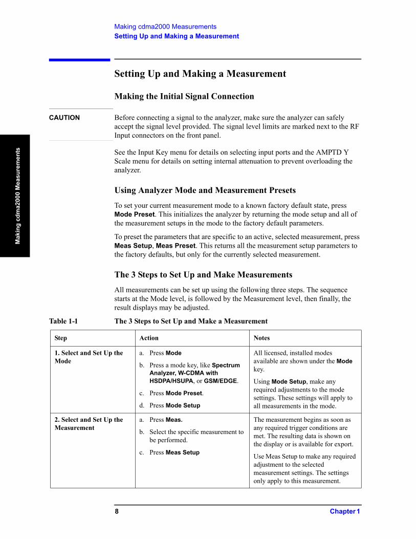
All measurements can be set up using the following three steps. The sequence starts at the Mode level, is followed by the Measurement level, then finally, the result displays may be adjusted.
Table 1-1 The 3 Steps to Set Up and Make a Measurement
Step Action Notes
1. Select and Set Up the Mode
a. Press Mode
b. Press a mode key, like Spectrum Analyzer, W-CDMA with HSDPA/HSUPA, or GSM/EDGE.
c. Press Mode Preset.
d. Press Mode Setup
All licensed, installed modes available are shown under the Mode key.
Using Mode Setup, make any required adjustments to the mode settings. These settings will apply to all measurements in the mode.
2. Select and Set Up the Measurement
a. Press Meas.
b. Select the specific measurement to be performed.
c. Press Meas Setup
The measurement begins as soon as any required trigger conditions are met. The resulting data is shown on the display or is available for export.
Use Meas Setup to make any required adjustment to the selected measurement settings. The settings only apply to this measurement.
8 Chapter 1

Making cdma2000 MeasurementsSetting Up and Making a Measurement
Making cdm
a2000 Measurem
ents
NOTE A setting may be reset at any time, and will be in effect on the next measurement cycle or view.
3. Select and Set Up a View of the Results
Press View/Display. Select a display format for the current measurement data.
Depending on the mode and measurement selected, other graphical and tabular data presentations may be available. X-Scale and Y-Scale adjustments may also be made now.
Table 1-2 Main Keys and Functions for Making Measurements
Step Primary Key Setup Keys Related Keys
1. Select and set up a mode. Mode Mode Setup, FREQ Channel
System
2. Select and set up a measurement. Meas Meas Setup Sweep/Control, Restart, Single, Cont
3. Select and set up a view of the results.
View/Display SPAN X Scale, AMPTD Y Scale
Peak Search,Quick Save, Save, Recall, File, Print
Table 1-1 The 3 Steps to Set Up and Make a Measurement
Step Action Notes
Chapter 1 9

Making cdma2000 MeasurementsSetting Up and Making a Measurement
Mak
ing
cdm
a200
0 M
easu
rem
ents
10 Chapter 1
2 Channel Power Measurements
This chapter explains how to make a channel power measurement on a cdma2000 mobile station (MS). This test measures the total RF power present in the channel. The results are shown in a graph window and in a text window.
11
Channel Power MeasurementsSetting Up and Making a Measurement
Cha
nnel
Pow
er M
easu
rem
ents
Setting Up and Making a Measurement
Configuring the Measurement System
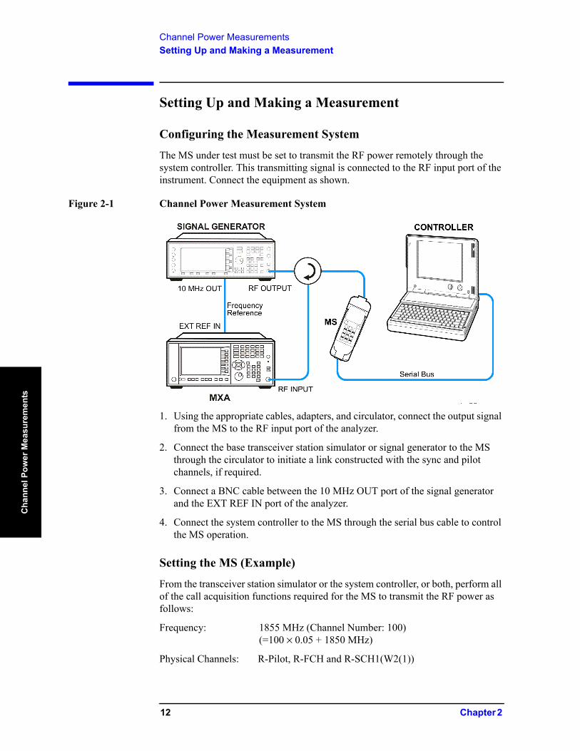
The MS under test must be set to transmit the RF power remotely through the system controller. This transmitting signal is connected to the RF input port of the instrument. Connect the equipment as shown.
Figure 2-1 Channel Power Measurement System
1. Using the appropriate cables, adapters, and circulator, connect the output signal from the MS to the RF input port of the analyzer.
2. Connect the base transceiver station simulator or signal generator to the MS through the circulator to initiate a link constructed with the sync and pilot channels, if required.
3. Connect a BNC cable between the 10 MHz OUT port of the signal generator and the EXT REF IN port of the analyzer.
4. Connect the system controller to the MS through the serial bus cable to control the MS operation.
Setting the MS (Example)
From the transceiver station simulator or the system controller, or both, perform all of the call acquisition functions required for the MS to transmit the RF power as follows:
Frequency: 1855 MHz (Channel Number: 100)(=100 × 0.05 + 1850 MHz)
Physical Channels: R-Pilot, R-FCH and R-SCH1(W2(1))
12 Chapter 2
Channel Power MeasurementsSetting Up and Making a Measurement
Channel Pow
er Measurem
ents
Output Power: –20 dBm (at analyzer input)
Measurement Procedure
Step 1. Enable the cdma2000 measurements.
Press Mode, cdma2000
Step 2. Preset the Mode.
Press Mode Preset.
Step 3. Toggle the device.
Press Mode Setup, Radio, Device to select the device to MS.
Step 4. Set the center frequency.
Press FREQ Channel, 1855, MHz.
Step 5. Initiate the channel power measurement.
Press Meas, Channel Power.
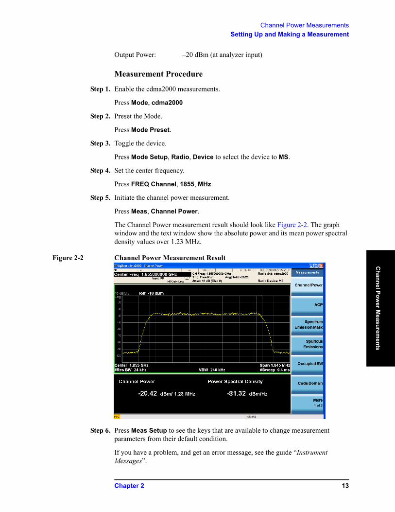
The Channel Power measurement result should look like Figure 2-2. The graph window and the text window show the absolute power and its mean power spectral density values over 1.23 MHz.
Figure 2-2 Channel Power Measurement Result
Step 6. Press Meas Setup to see the keys that are available to change measurement parameters from their default condition.
If you have a problem, and get an error message, see the guide “Instrument Messages”.
Chapter 2 13
Channel Power MeasurementsSetting Up and Making a Measurement
Cha
nnel
Pow
er M
easu
rem
ents
14 Chapter 2
3 ACP Measurements
This chapter explains how to make the adjacent channel leakage power ratio (ACLR or ACPR) measurement on a cdma2000 mobile station (MS). ACPR is a measurement of the amount of interference, or power, in an adjacent frequency channel. The results are displayed as a bar graph or as spectrum data, with measurement data at specified offsets.
15
ACP MeasurementsSetting Up and Making a Measurement
AC
P M
easu
rem
ents
Setting Up and Making a Measurement
Configuring the Measurement System
The MS under test must be set to transmit the RF power remotely through the system controller. This transmitting signal is connected to the RF input port of the instrument. Connect the equipment as shown.
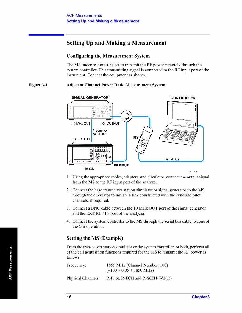
Figure 3-1 Adjacent Channel Power Ratio Measurement System
1. Using the appropriate cables, adapters, and circulator, connect the output signal from the MS to the RF input port of the analyzer.
2. Connect the base transceiver station simulator or signal generator to the MS through the circulator to initiate a link constructed with the sync and pilot channels, if required.
3. Connect a BNC cable between the 10 MHz OUT port of the signal generator and the EXT REF IN port of the analyzer.
4. Connect the system controller to the MS through the serial bus cable to control the MS operation.
Setting the MS (Example)
From the transceiver station simulator or the system controller, or both, perform all of the call acquisition functions required for the MS to transmit the RF power as follows:
Frequency: 1855 MHz (Channel Number: 100)(=100 × 0.05 + 1850 MHz)
Physical Channels: R-Pilot, R-FCH and R-SCH1(W2(1))
16 Chapter 3

ACP MeasurementsSetting Up and Making a Measurement
AC
P Measurem
ents
Output Power: –20 dBm (at analyzer input)
Measurement Procedure
Step 1. Enable the cdma2000 measurements.
Press Mode, cdma2000.
Step 2. Preset the mode.
Press Mode Preset.
Step 3. Select the device.
Press Mode Setup, Radio, Device to select the device to MS.
Step 4. Set the center frequency.
Press FREQ Channel, 1855, MHz.
Step 5. Initiate the adjacent channel leakage power ratio measurement.
Press Meas, ACP.
Figure 3-2 Measurement Result - ACP-RBW View (Default)
NOTE You can zoom on either the numeric or the graphic result by pressing Window Control Keys which are at the bottom of the screen.
Step 6. Press Meas Setup, More, Meas Method, IBW to see the bar graph with the spectrum trace graph overlay. The spectrum graph measurement result should look like Figure 3-3. The graph (referenced to the total power) and a text window are displayed. The text window shows the absolute total power reference, while the
Chapter 3 17
ACP MeasurementsSetting Up and Making a Measurement
AC
P M
easu
rem
ents
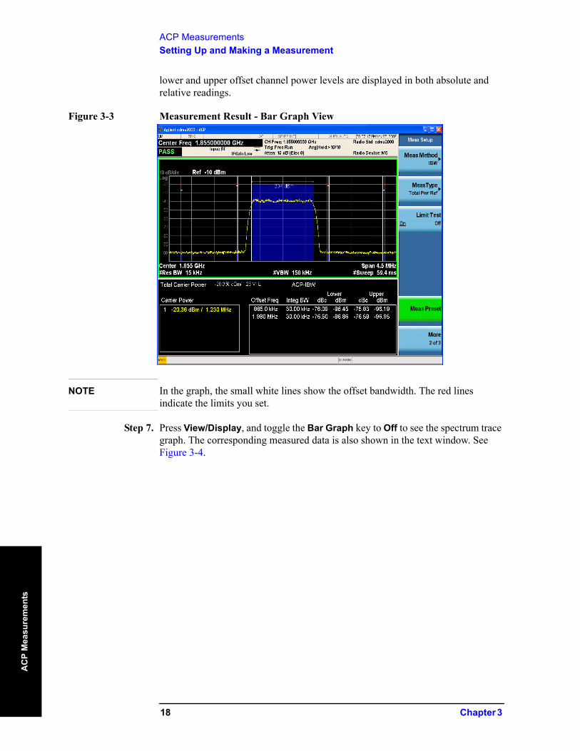
lower and upper offset channel power levels are displayed in both absolute and relative readings.
Figure 3-3 Measurement Result - Bar Graph View
NOTE In the graph, the small white lines show the offset bandwidth. The red lines indicate the limits you set.
Step 7. Press View/Display, and toggle the Bar Graph key to Off to see the spectrum trace graph. The corresponding measured data is also shown in the text window. See Figure 3-4.
18 Chapter 3
ACP MeasurementsSetting Up and Making a Measurement
AC
P Measurem
ents
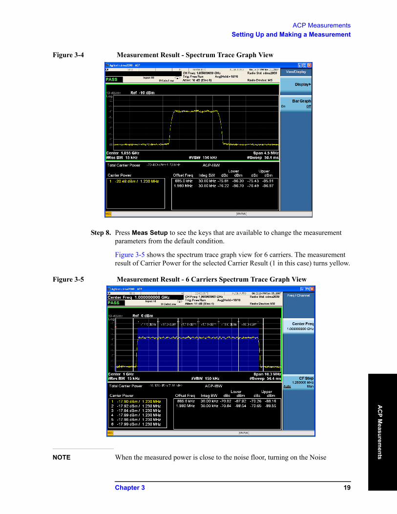
Figure 3-4 Measurement Result - Spectrum Trace Graph View
Step 8. Press Meas Setup to see the keys that are available to change the measurement parameters from the default condition.
Figure 3-5 shows the spectrum trace graph view for 6 carriers. The measurement result of Carrier Power for the selected Carrier Result (1 in this case) turns yellow.
Figure 3-5 Measurement Result - 6 Carriers Spectrum Trace Graph View
NOTE When the measured power is close to the noise floor, turning on the Noise
Chapter 3 19

ACP MeasurementsSetting Up and Making a Measurement
AC
P M
easu
rem
ents
Correction under the Meas Setup menu can make the measurement more accurate.
If you have a problem, and get an error message, see the guide “Instrument Messages”.
20 Chapter 3

4 Spectrum Emission Mask Measurements
This chapter explains how to make the spectrum emission mask (SEM) measurement on a cdma2000 mobile station (MS). SEM compares the total power level within the defined carrier bandwidth and the given offset channels on both sides of the carrier frequency, to levels allowed by the standard. Results of the measurement of each offset segment can be viewed separately.21
Spectrum Emission Mask MeasurementsSetting Up and Making a Measurement
Spec
trum
Em
issi
on M
ask
Mea
sure
men
ts
Setting Up and Making a Measurement
Configuring the Measurement System
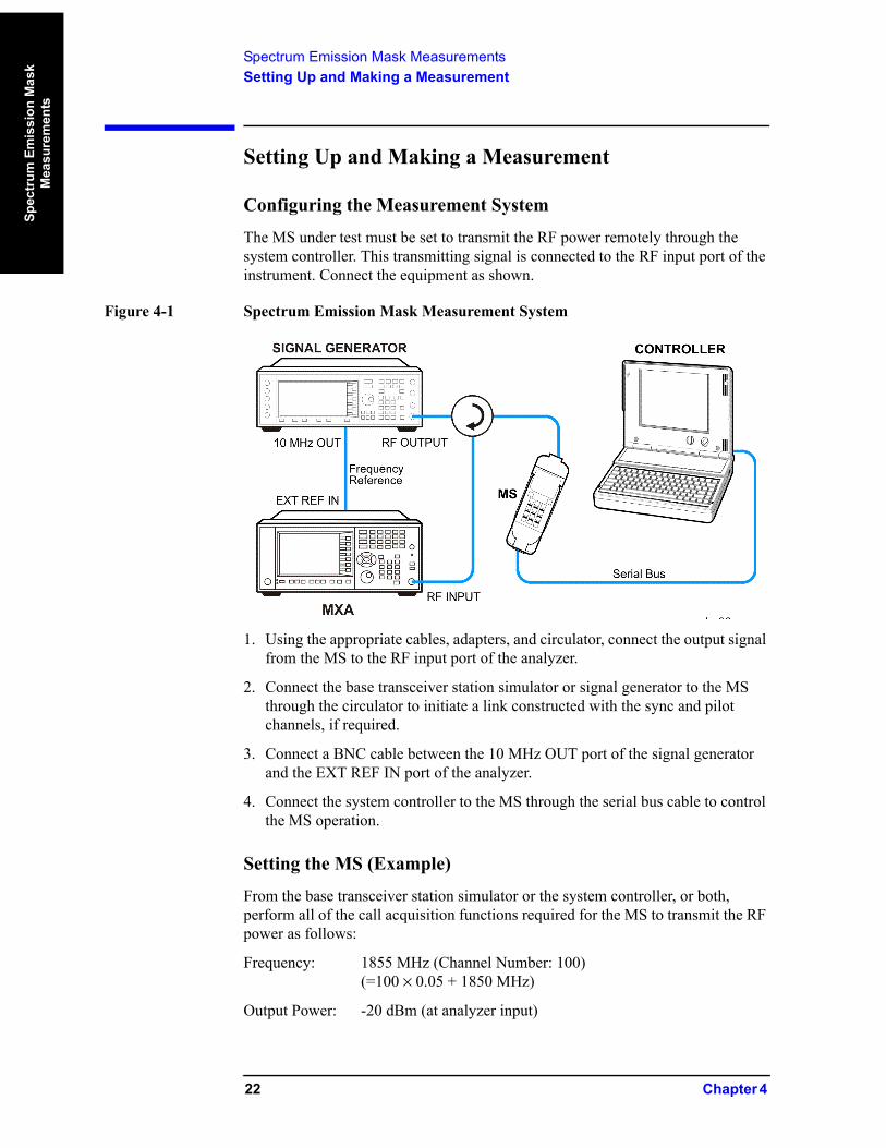
The MS under test must be set to transmit the RF power remotely through the system controller. This transmitting signal is connected to the RF input port of the instrument. Connect the equipment as shown.
Figure 4-1 Spectrum Emission Mask Measurement System
1. Using the appropriate cables, adapters, and circulator, connect the output signal from the MS to the RF input port of the analyzer.
2. Connect the base transceiver station simulator or signal generator to the MS through the circulator to initiate a link constructed with the sync and pilot channels, if required.
3. Connect a BNC cable between the 10 MHz OUT port of the signal generator and the EXT REF IN port of the analyzer.
4. Connect the system controller to the MS through the serial bus cable to control the MS operation.
Setting the MS (Example)
From the base transceiver station simulator or the system controller, or both, perform all of the call acquisition functions required for the MS to transmit the RF power as follows:
Frequency: 1855 MHz (Channel Number: 100)(=100 × 0.05 + 1850 MHz)
Output Power: -20 dBm (at analyzer input)
22 Chapter 4
Spectrum Emission Mask MeasurementsSetting Up and Making a Measurement
Spectrum Em
ission Mask
Measurem
ents
Measurement Procedure
Step 1. Enable the cdma2000 measurements.
Press Mode, cdma2000.
Step 2. Preset the mode.
Press Mode Preset.
Step 3. Select the device to MS.
Press Mode Setup, Radio, Device and toggle the device to MS.
Step 4. Set the center frequency.
Press FREQ Channel, 1855, MHz.
Step 5. Initiate the spectrum emission mask measurement.
Press Meas, Spectrum Emission Mask.
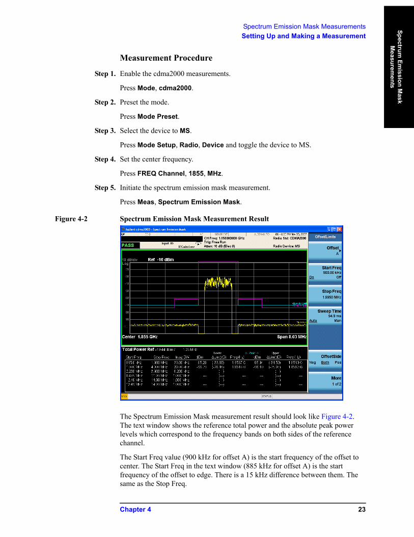
Figure 4-2 Spectrum Emission Mask Measurement Result
The Spectrum Emission Mask measurement result should look like Figure 4-2. The text window shows the reference total power and the absolute peak power levels which correspond to the frequency bands on both sides of the reference channel.
The Start Freq value (900 kHz for offset A) is the start frequency of the offset to center. The Start Freq in the text window (885 kHz for offset A) is the start frequency of the offset to edge. There is a 15 kHz difference between them. The same as the Stop Freq.
Chapter 4 23
Spectrum Emission Mask MeasurementsSetting Up and Making a Measurement
Spec
trum
Em
issi
on M
ask
Mea
sure
men
ts
The Lower or Upper Lim is the minimum margin from limit line which is decided by Fail Mask setting. There are four settings for Fail Mask: Absolute, Relative, Abs AND Rel, Abs OR Rel.
• For Absolute mask, the Lower or Upper Lim is compared with the Absolute Limit line.
• For Relative mask, the Lower or Upper Lim is compared with the Relative Limit line.
• For Abs AND Rel mask, the Lower or Upper Lim is compared with the higher Limit line.
• For Abs OR Rel mask, the Lower or Upper Lim is compared with the lower Limit line.
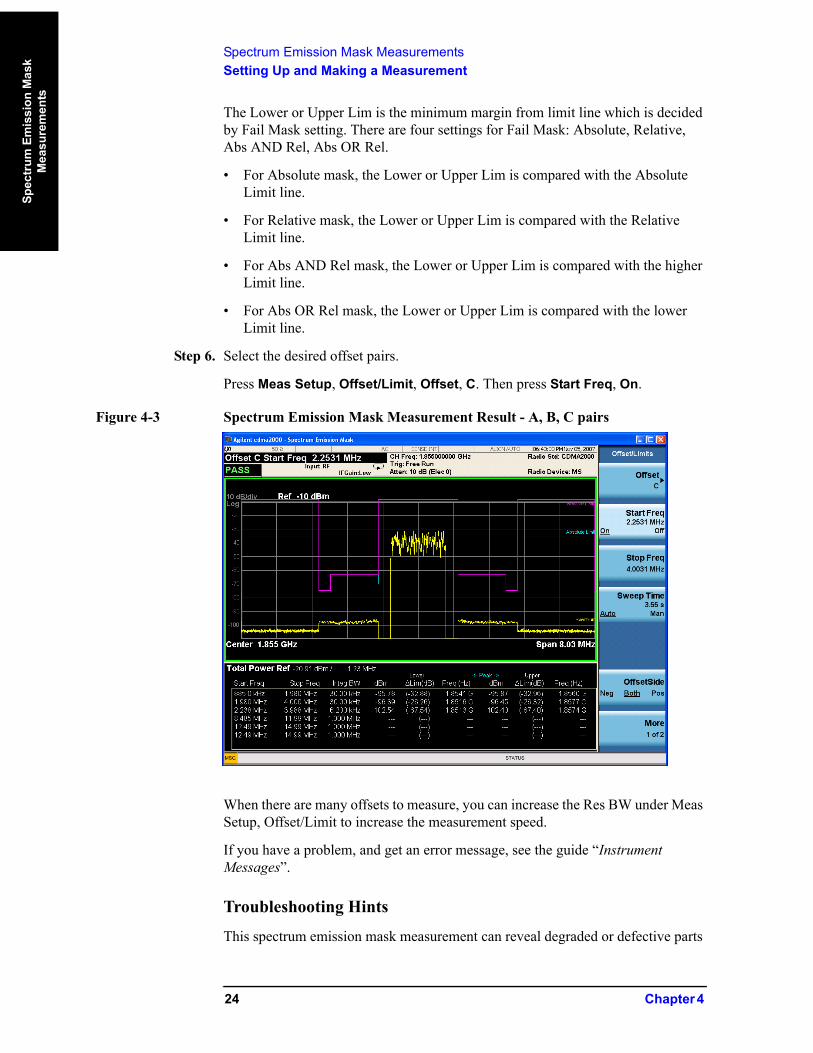
Step 6. Select the desired offset pairs.
Press Meas Setup, Offset/Limit, Offset, C. Then press Start Freq, On.
Figure 4-3 Spectrum Emission Mask Measurement Result - A, B, C pairs
When there are many offsets to measure, you can increase the Res BW under Meas Setup, Offset/Limit to increase the measurement speed.
If you have a problem, and get an error message, see the guide “Instrument Messages”.
Troubleshooting Hints
This spectrum emission mask measurement can reveal degraded or defective parts
24 Chapter 4

Spectrum Emission Mask MeasurementsSetting Up and Making a Measurement
Spectrum Em
ission Mask
Measurem
ents
in the transmitter section of the unit under test (UUT). The following examples are those areas to be checked further.
• Faulty DC power supply control of the transmitter power amplifier.
• RF power controller of the pre-power amplifier stage.
• I/Q control of the baseband stage.
• Degradation in the gain and output power level of the amplifier due to the degraded gain control or increased distortion, or both.
• Degradation of the amplifier linearity or other performance characteristics.
Power amplifiers are one of the final stage elements of a base or mobile transmitter and are a critical part of meeting the important power and spectral efficiency specifications. Since spectrum emission mask measures the spectral response of the amplifier to a complex wideband signal, it is a key measurement linking amplifier linearity and other performance characteristics to the stringent system specifications.
Chapter 4 25

Spectrum Emission Mask MeasurementsSetting Up and Making a Measurement
Spec
trum
Em
issi
on M
ask
Mea
sure
men
ts
26 Chapter 4

5 Spurious Emissions Measurement
This section explains how to make the spurious emission measurement on a cdma2000 mobile station (MS).This measurement identifies and determines the power level of spurious emissions in certain frequency bands.
27
Spurious Emissions MeasurementSetting Up and Making a Measurement
Spur
ious
Em
issi
ons
Mea
sure
men
t
Setting Up and Making a Measurement
Configuring the Measurement System
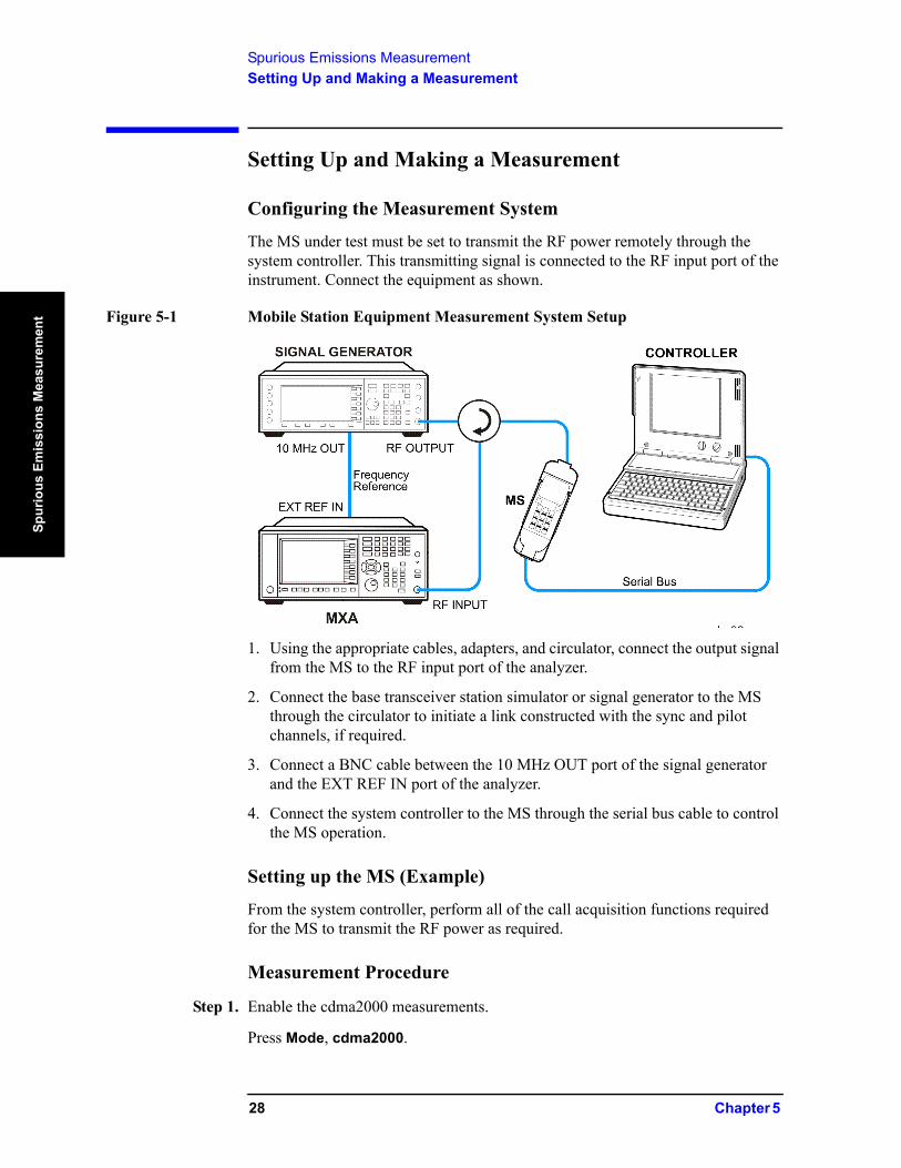
The MS under test must be set to transmit the RF power remotely through the system controller. This transmitting signal is connected to the RF input port of the instrument. Connect the equipment as shown.
Figure 5-1 Mobile Station Equipment Measurement System Setup
1. Using the appropriate cables, adapters, and circulator, connect the output signal from the MS to the RF input port of the analyzer.
2. Connect the base transceiver station simulator or signal generator to the MS through the circulator to initiate a link constructed with the sync and pilot channels, if required.
3. Connect a BNC cable between the 10 MHz OUT port of the signal generator and the EXT REF IN port of the analyzer.
4. Connect the system controller to the MS through the serial bus cable to control the MS operation.
Setting up the MS (Example)
From the system controller, perform all of the call acquisition functions required for the MS to transmit the RF power as required.
Measurement Procedure
Step 1. Enable the cdma2000 measurements.
Press Mode, cdma2000.
28 Chapter 5
Spurious Emissions MeasurementSetting Up and Making a Measurement
Spurious Emissions M
easurement
Step 2. Preset the mode.
Press Mode Preset.
Step 3. Toggle the RF Coupling to DC.
Press Input/Output, RF Input, RF Coupling, DC.
NOTE In AC coupling mode, you can view signals less than 10 MHz but the amplitude accuracy is not specified. To accurately see a signal of less than 10 MHz, you must switch to DC coupling.
When operating in DC coupled mode, ensure protection of the External Mixer by limiting the DC part of the input level to within 200 mV of 0 Vdc.
Step 4. Select the device to MS.
Press Mode Setup, Radio, Device, MS.
Step 5. Enter the center frequency.
Press FREQ Channel, enter a numerical frequency using the front-panel keypad, and select a units key, such as MHz.
Step 6. Initiate the spurious emission measurement.
Press Meas, Spurious Emission.
Depending on the current settings, the instrument will begin making the selected measurements. The resulting data is shown on the display or available for export.
Step 7. Setup the Range Table.
Press Meas Setup, Range Table.
You can enter the settings for up to twenty ranges. Press Meas Setup to returen the screen from range table to spur table.
If you want to change the measurement parameters from other default condition for a customized measurement, press Meas Setup to see the parameter keys that are available.
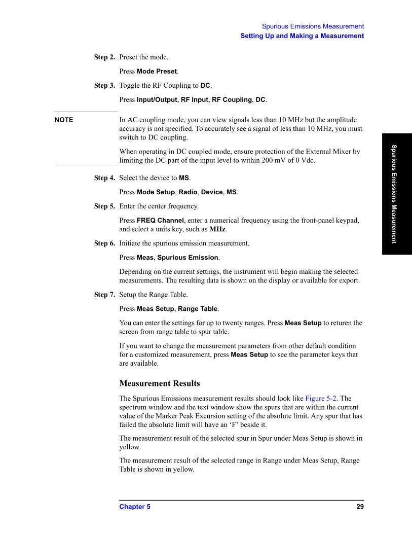
Measurement Results
The Spurious Emissions measurement results should look like Figure 5-2. The spectrum window and the text window show the spurs that are within the current value of the Marker Peak Excursion setting of the absolute limit. Any spur that has failed the absolute limit will have an ‘F’ beside it.
The measurement result of the selected spur in Spur under Meas Setup is shown in yellow.
The measurement result of the selected range in Range under Meas Setup, Range Table is shown in yellow.
Chapter 5 29

Spurious Emissions MeasurementSetting Up and Making a Measurement
Spur
ious
Em
issi
ons
Mea
sure
men
t
Figure 5-2 Spurious Emissions Measurement
NOTE If you set the Meas Type to Examine, the trace is kept updating to show the latest spectrum where the range which has the worst spurious. However, the table is shown the last report. Press Restart to update the table to show the latest result.
For the Meas Type of Examine, if you want to see the measurement result for different ranges, you can pressMeas Setup, Range Table, Range, then enter the range number you care.
You can use the window control keys below the screen to zoom the result screen. See Figure 5-3.
30 Chapter 5
Spurious Emissions MeasurementSetting Up and Making a Measurement
Spurious Emissions M
easurement
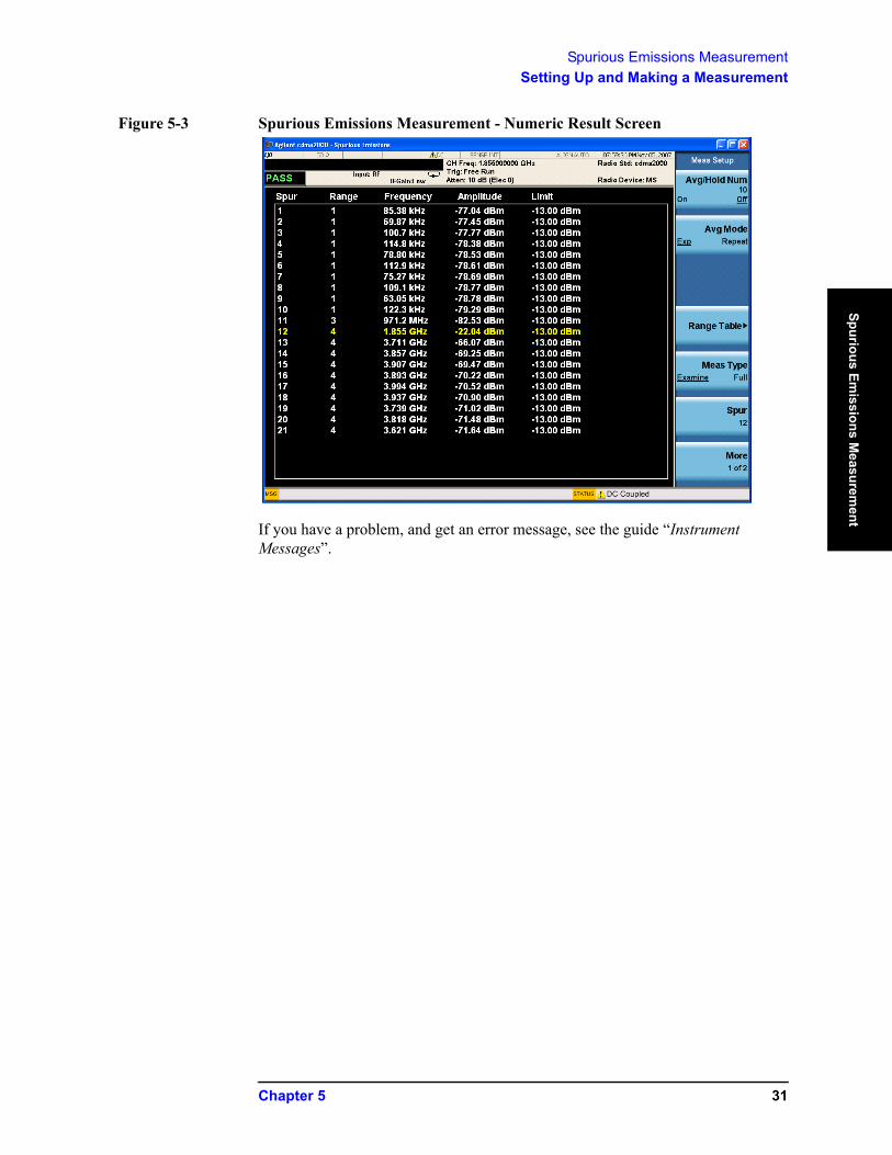
Figure 5-3 Spurious Emissions Measurement - Numeric Result Screen
If you have a problem, and get an error message, see the guide “Instrument Messages”.
Chapter 5 31

Spurious Emissions MeasurementSetting Up and Making a Measurement
Spur
ious
Em
issi
ons
Mea
sure
men
t
32 Chapter 5
6 Occupied Bandwidth Measurements
This chapter explains how to make the occupied bandwidth measurement on a cdma2000 mobile station (MS). The instrument measures power across the band, and then calculates its 99.0% power bandwidth.
33

Occupied Bandwidth MeasurementsSetting Up and Making a Measurement
Occ
upie
d B
andw
idth
Mea
sure
men
ts
Setting Up and Making a Measurement
Configuring the Measurement System
The MS under test must be set to transmit the RF power remotely through the system controller. This transmitting signal is connected to the RF input port of the instrument. Connect the equipment as shown.
Figure 6-1 Occupied Bandwidth Measurement System
1. Using the appropriate cables, adapters, and circulator, connect the output signal of the MS to the RF input of the analyzer.
2. Connect the base transceiver station simulator or signal generator to the MS through the circulator to initiate a link constructed with the sync and pilot channels, if required.
3. Connect a BNC cable between the 10 MHz OUT port of the signal generator and the EXT REF IN port of the analyzer.
4. Connect the system controller to the MS through the serial bus cable to control the MS operation.
Setting the MS (Example)
From the base transceiver station simulator or the system controller, or both, perform all of the call acquisition functions required for the MS to transmit the RF power as follows:
Frequency: 1855 MHz (Channel Number: 100)(=100 × 0.05 + 1850 MHz)
Output Power: –20 dBm (or other power level for the MS)
34 Chapter 6
Occupied Bandwidth MeasurementsSetting Up and Making a Measurement
Occupied B
andwidth M
easurements
Measurement Procedure
Step 1. Enable the cdma2000 measurements.
Press Mode, cdma2000.
Step 2. Preset the mode.
Press Mode Preset.
Step 3. Toggle the device to MS.
Press Mode Setup, Radio, Device, MS.
Step 4. Set the center frequency to 1.855 GHz.
Press FREQ Channel, 1855, MHz.
Step 5. Initiate the occupied bandwidth measurement.
Press Meas, Occupied BW.
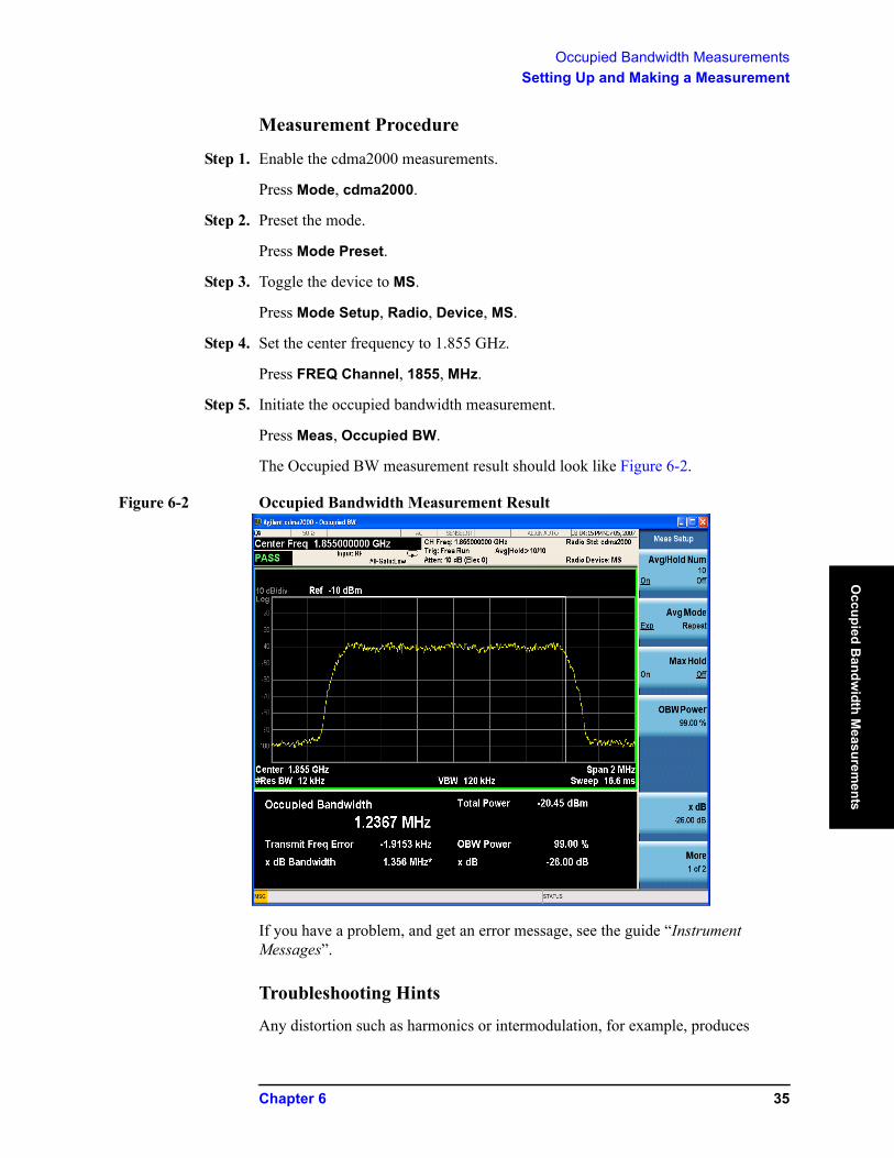
The Occupied BW measurement result should look like Figure 6-2.
Figure 6-2 Occupied Bandwidth Measurement Result
If you have a problem, and get an error message, see the guide “Instrument Messages”.
Troubleshooting Hints
Any distortion such as harmonics or intermodulation, for example, produces
Chapter 6 35
Occupied Bandwidth MeasurementsSetting Up and Making a Measurement
Occ
upie
d B
andw
idth
Mea
sure
men
ts
undesirable power outside the specified bandwidth.
Shoulders on either side of the spectrum shape indicate spectral regrowth and intermodulation. Rounding or sloping of the top shape can indicate filter shape problems.
36 Chapter 6
7 Code Domain Measurements
This chapter explains how to make a code domain measurement on a cdma2000 mobile station (MS) and a base transceiver station (BTS). This is the measurement of power levels of the spread code channels across composite RF channels, relative to the total power within the 1.23 MHz channel bandwidth centered at the center frequency.
37
Code Domain MeasurementsSetting Up and Making a Measurement
Cod
e D
omai
n M
easu
rem
ents
Setting Up and Making a Measurement
cdma2000 Measurement Example (MS)
Configuring the Measurement System
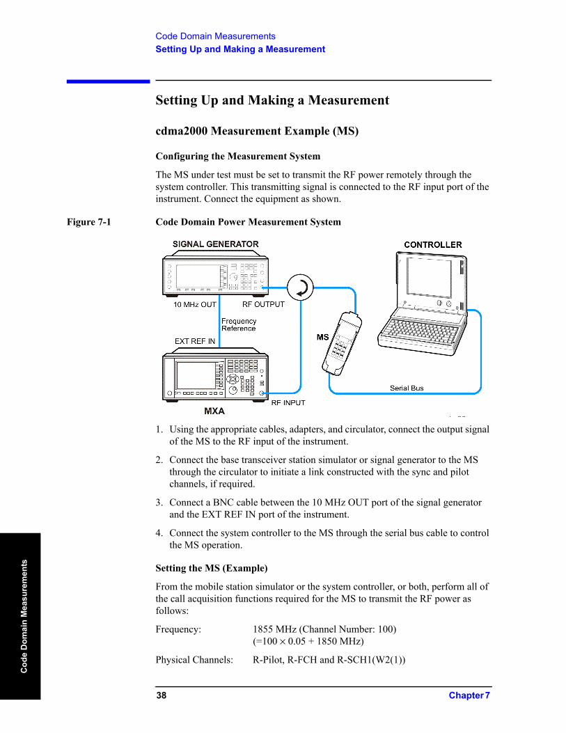
The MS under test must be set to transmit the RF power remotely through the system controller. This transmitting signal is connected to the RF input port of the instrument. Connect the equipment as shown.
Figure 7-1 Code Domain Power Measurement System
1. Using the appropriate cables, adapters, and circulator, connect the output signal of the MS to the RF input of the instrument.
2. Connect the base transceiver station simulator or signal generator to the MS through the circulator to initiate a link constructed with the sync and pilot channels, if required.
3. Connect a BNC cable between the 10 MHz OUT port of the signal generator and the EXT REF IN port of the instrument.
4. Connect the system controller to the MS through the serial bus cable to control the MS operation.
Setting the MS (Example)
From the mobile station simulator or the system controller, or both, perform all of the call acquisition functions required for the MS to transmit the RF power as follows:
Frequency: 1855 MHz (Channel Number: 100)(=100 × 0.05 + 1850 MHz)
Physical Channels: R-Pilot, R-FCH and R-SCH1(W2(1))
38 Chapter 7

Code Domain MeasurementsSetting Up and Making a Measurement
Code D
omain M
easurements
Long Code Mask: 0000000000
Output Power: –20 dBm (at analyzer input)
Measurement Procedure
Step 1. Enable the cdma2000 measurements.
Press Mode, cdma2000.
Step 2. Preset the mode.
Press Mode Preset.
Step 3. Select the device to MS.
Press Mode Setup, Radio, Device to toggle the device to MS.
Step 4. Set the center frequency.
Press FREQ Channel, 1855, MHz.
Step 5. Initiate the code domain measurement.
Press Meas, Code Domain.
The measurement result should look like Figure 7-2. The graph window is displayed with a text window below it. The text window shows the total power level along with the relative power levels of the various channels.
Figure 7-2 Code Domain Measurement Result - Power Graph & Metrics (Default) View
Step 6. Press Peak Search, Next Peak. Because the Consolidated Marker (under View/Display, Power Graph & Metrics menu) is On, the Walsh code channel with
Chapter 7 39
Code Domain MeasurementsSetting Up and Making a Measurement
Cod
e D
omai
n M
easu
rem
ents
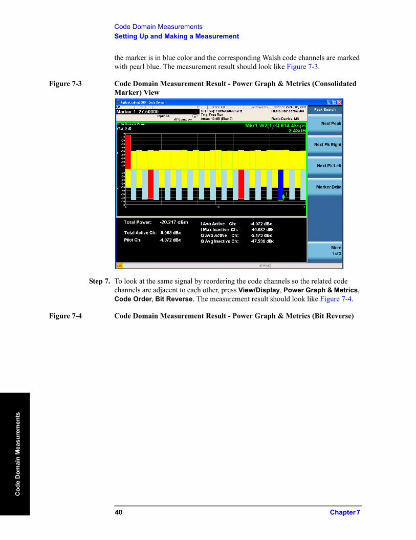
the marker is in blue color and the corresponding Walsh code channels are marked with pearl blue. The measurement result should look like Figure 7-3.
Figure 7-3 Code Domain Measurement Result - Power Graph & Metrics (Consolidated Marker) View
Step 7. To look at the same signal by reordering the code channels so the related code channels are adjacent to each other, press View/Display, Power Graph & Metrics, Code Order, Bit Reverse. The measurement result should look like Figure 7-4.
Figure 7-4 Code Domain Measurement Result - Power Graph & Metrics (Bit Reverse)
40 Chapter 7
Code Domain MeasurementsSetting Up and Making a Measurement
Code D
omain M
easurements
View
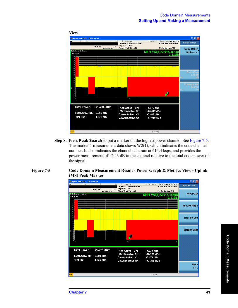
Step 8. Press Peak Search to put a marker on the highest power channel. See Figure 7-5. The marker 1 measurement data shows W2(1), which indicates the code channel number. It also indicates the channel data rate at 614.4 ksps, and provides the power measurement of –2.43 dB in the channel relative to the total code power of the signal.
Figure 7-5 Code Domain Measurement Result - Power Graph & Metrics View - Uplink (MS) Peak Marker
Chapter 7 41
Code Domain MeasurementsSetting Up and Making a Measurement
Cod
e D
omai
n M
easu
rem
ents
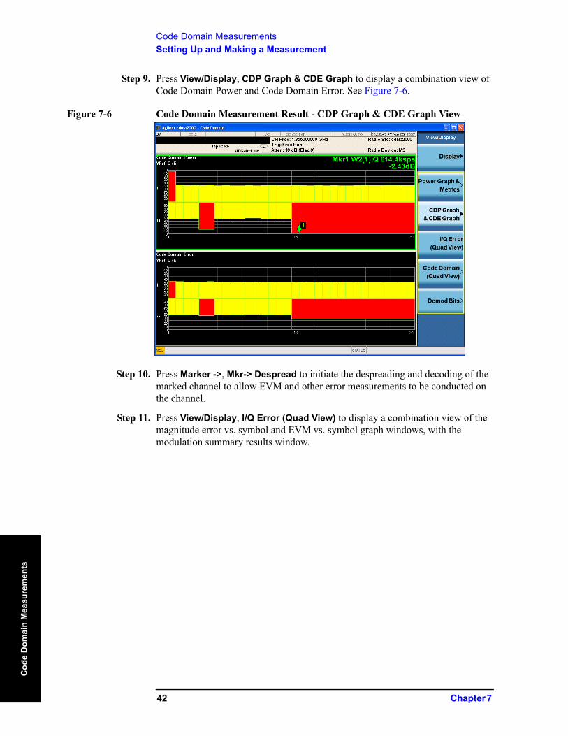
Step 9. Press View/Display, CDP Graph & CDE Graph to display a combination view of Code Domain Power and Code Domain Error. See Figure 7-6.
Figure 7-6 Code Domain Measurement Result - CDP Graph & CDE Graph View
Step 10. Press Marker ->, Mkr-> Despread to initiate the despreading and decoding of the marked channel to allow EVM and other error measurements to be conducted on the channel.
Step 11. Press View/Display, I/Q Error (Quad View) to display a combination view of the magnitude error vs. symbol and EVM vs. symbol graph windows, with the modulation summary results window.
42 Chapter 7
Code Domain MeasurementsSetting Up and Making a Measurement
Code D
omain M
easurements
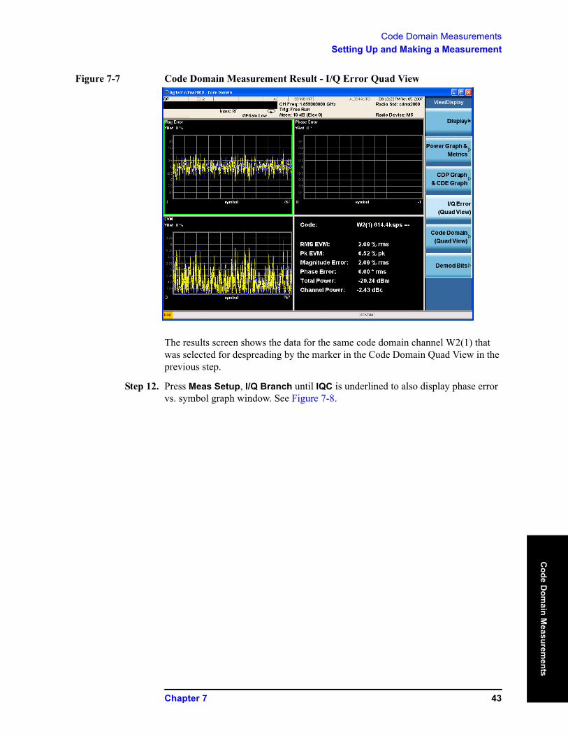
Figure 7-7 Code Domain Measurement Result - I/Q Error Quad View
The results screen shows the data for the same code domain channel W2(1) that was selected for despreading by the marker in the Code Domain Quad View in the previous step.
Step 12. Press Meas Setup, I/Q Branch until IQC is underlined to also display phase error vs. symbol graph window. See Figure 7-8.
Chapter 7 43

Code Domain MeasurementsSetting Up and Making a Measurement
Cod
e D
omai
n M
easu
rem
ents
Figure 7-8 Code Domain Measurement Result - I/Q Error Quad View (with phase error)
Step 13. Press View/Display, Code Domain (Quad View) to display a combination view of the code domain power, symbol power, and I/Q symbol polar vector graph windows, with a summary results window. See Figure 7-9.
Figure 7-9 Code Domain Measurement Result - Code Domain Quad View
44 Chapter 7
Code Domain MeasurementsSetting Up and Making a Measurement
Code D
omain M
easurements
In Figure 7-9, the original Code Domain Measurement is shown at the top left, while the Symbol Power measurement of the marked Q-data channel is at the top right (You can select I-data, Q-data or combined I and Q data in the I/Q Branch of Meas Setup). The solid area below the first graticule (blue on the instrument display) is the composite chip power versus time over the entire capture interval, while the yellow area is symbol power versus time for W2(1). The Capture Interval is 5 PCG, but the measured interval is 1 PCG (if there is only 1 PCG for the measured interval, it is marked with red vertical lines, if there are several PCG, the first measured PCG is marked with red vertical lines, and there is a white vertical line for the others). The Capture Interval and the Meas Interval can be set in the Meas Setup menu.
The graph of the I/Q vector trajectory for W2(1) during the measurement interval is shown at the lower left. As the constellation diagram shows, this example uses Q-only data that is effectively BPSK modulation for channel W2(1), so the phase error must be zero.
The summary data at the lower right indicates peak and RMS EVM, magnitude and phase errors, powers of the signal and the channel.
NOTE You can use the Composite Chip Power key (in the View Settings of Code Domain (Quad View)) to switch the composite chip power display function between On and Off.
Under the View/Display menu, there are arrows in the right side of some keys like Code Domain (Quad View). The first time you press this kind of key means this view is selected, the hollow arrow turns solid, and the second time you press it, the view settings of this view are displayed.
Step 14. Press View/Display, Demod Bits to display a combination view of the code domain power, symbol power graph windows, and the I/Q demodulated bit stream data for the symbol power slots selected by the measurement interval and measurement offset parameters.
Chapter 7 45
Code Domain MeasurementsSetting Up and Making a Measurement
Cod
e D
omai
n M
easu
rem
ents
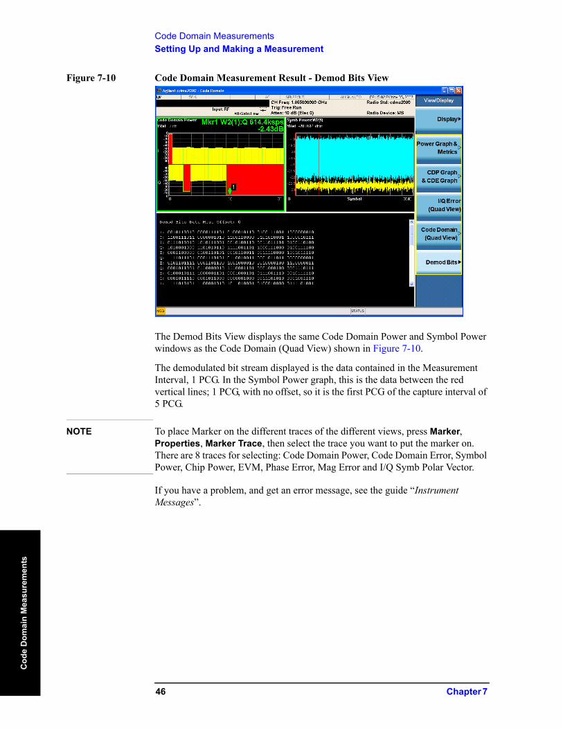
Figure 7-10 Code Domain Measurement Result - Demod Bits View
The Demod Bits View displays the same Code Domain Power and Symbol Power windows as the Code Domain (Quad View) shown in Figure 7-10.
The demodulated bit stream displayed is the data contained in the Measurement Interval, 1 PCG. In the Symbol Power graph, this is the data between the red vertical lines; 1 PCG, with no offset, so it is the first PCG of the capture interval of 5 PCG.
NOTE To place Marker on the different traces of the different views, press Marker, Properties, Marker Trace, then select the trace you want to put the marker on. There are 8 traces for selecting: Code Domain Power, Code Domain Error, Symbol Power, Chip Power, EVM, Phase Error, Mag Error and I/Q Symb Polar Vector.
If you have a problem, and get an error message, see the guide “Instrument Messages”.
46 Chapter 7
Code Domain MeasurementsSetting Up and Making a Measurement
Code D
omain M
easurements
cdma2000 Measurement Example (BTS)
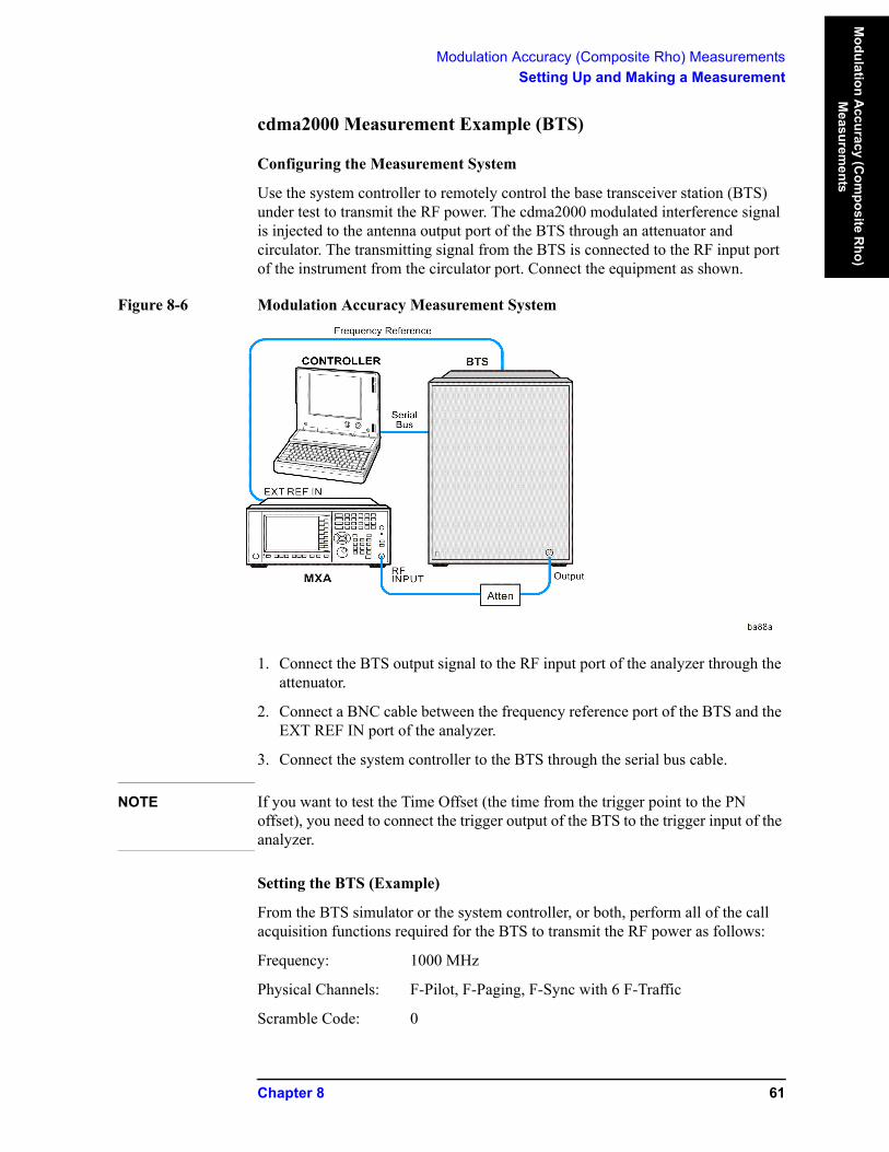
Configuring the Measurement System
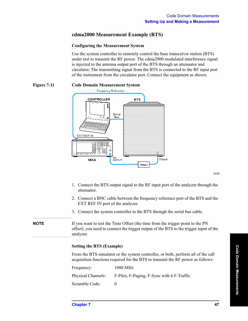
Use the system controller to remotely control the base transceiver station (BTS) under test to transmit the RF power. The cdma2000 modulated interference signal is injected to the antenna output port of the BTS through an attenuator and circulator. The transmitting signal from the BTS is connected to the RF input port of the instrument from the circulator port. Connect the equipment as shown.
Figure 7-11 Code Domain Measurement System
1. Connect the BTS output signal to the RF input port of the analyzer through the attenuator.
2. Connect a BNC cable between the frequency reference port of the BTS and the EXT REF IN port of the analyzer.
3. Connect the system controller to the BTS through the serial bus cable.
NOTE If you want to test the Time Offset (the time from the trigger point to the PN offset), you need to connect the trigger output of the BTS to the trigger input of the analyzer.
Setting the BTS (Example)
From the BTS simulator or the system controller, or both, perform all of the call acquisition functions required for the BTS to transmit the RF power as follows:
Frequency: 1000 MHz
Physical Channels: F-Pilot, F-Paging, F-Sync with 6 F-Traffic
Scramble Code: 0
Chapter 7 47
Code Domain MeasurementsSetting Up and Making a Measurement
Cod
e D
omai
n M
easu
rem
ents
Output Power: –10 dBm
Measurement Procedure
Step 1. Enable the cdma2000 measurements.
Press Mode, cdma2000.
Step 2. Preset the mode.
Press Mode Preset.
Step 3. Select the device to BTS.
Press Mode Setup, Radio, Device to toggle the device to BTS.
Step 4. Set the center frequency.
Press FREQ Channel, 1000, MHz.
Step 5. Initiate the code domain measurement.
Press Meas, Code Domain.
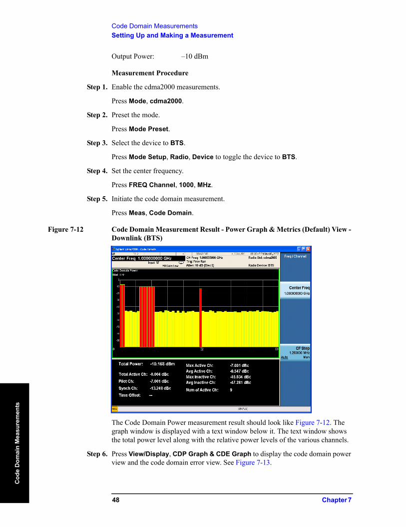
Figure 7-12 Code Domain Measurement Result - Power Graph & Metrics (Default) View - Downlink (BTS)
The Code Domain Power measurement result should look like Figure 7-12. The graph window is displayed with a text window below it. The text window shows the total power level along with the relative power levels of the various channels.
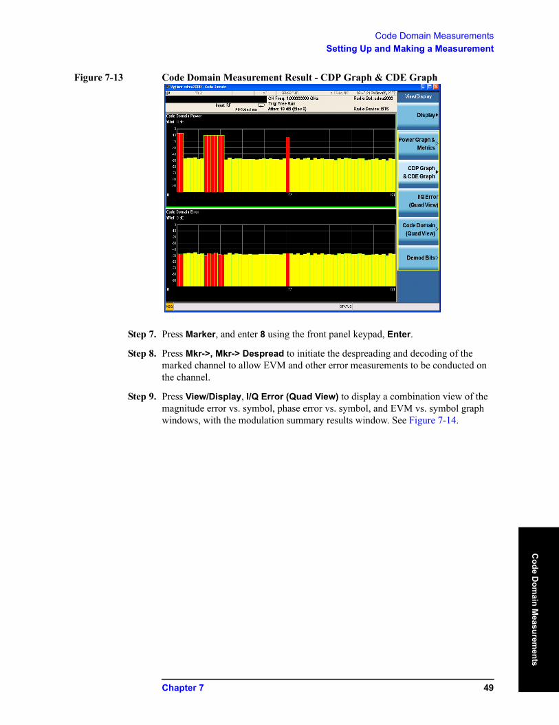
Step 6. Press View/Display, CDP Graph & CDE Graph to display the code domain power view and the code domain error view. See Figure 7-13.
48 Chapter 7
Code Domain MeasurementsSetting Up and Making a Measurement
Code D
omain M
easurements
Figure 7-13 Code Domain Measurement Result - CDP Graph & CDE Graph
Step 7. Press Marker, and enter 8 using the front panel keypad, Enter.
Step 8. Press Mkr->, Mkr-> Despread to initiate the despreading and decoding of the marked channel to allow EVM and other error measurements to be conducted on the channel.
Step 9. Press View/Display, I/Q Error (Quad View) to display a combination view of the magnitude error vs. symbol, phase error vs. symbol, and EVM vs. symbol graph windows, with the modulation summary results window. See Figure 7-14.
Chapter 7 49
Code Domain MeasurementsSetting Up and Making a Measurement
Cod
e D
omai
n M
easu
rem
ents
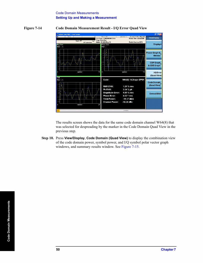
Figure 7-14 Code Domain Measurement Result - I/Q Error Quad View
The results screen shows the data for the same code domain channel W64(8) that was selected for despreading by the marker in the Code Domain Quad View in the previous step.
Step 10. Press View/Display, Code Domain (Quad View) to display the combination view of the code domain power, symbol power, and I/Q symbol polar vector graph windows, and summary results window. See Figure 7-15.
50 Chapter 7
Code Domain MeasurementsSetting Up and Making a Measurement
Code D
omain M
easurements
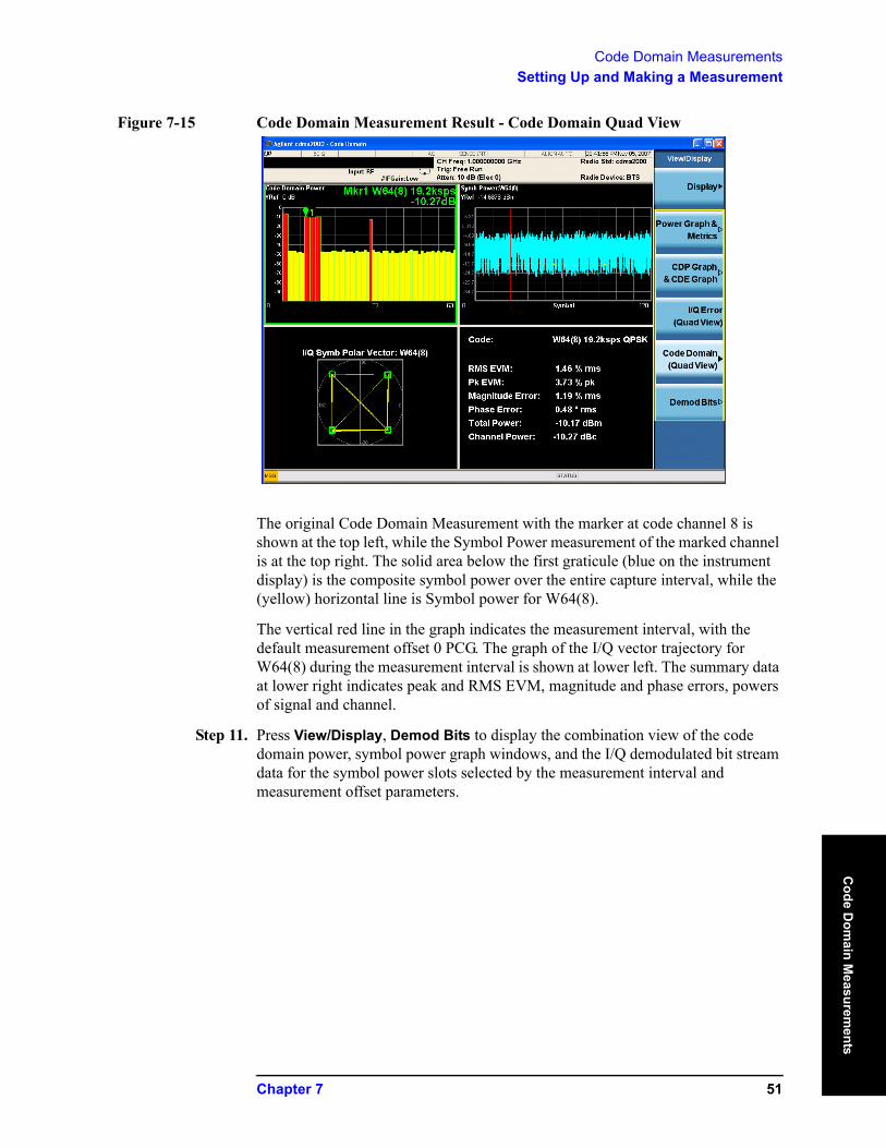
Figure 7-15 Code Domain Measurement Result - Code Domain Quad View
The original Code Domain Measurement with the marker at code channel 8 is shown at the top left, while the Symbol Power measurement of the marked channel is at the top right. The solid area below the first graticule (blue on the instrument display) is the composite symbol power over the entire capture interval, while the (yellow) horizontal line is Symbol power for W64(8).
The vertical red line in the graph indicates the measurement interval, with the default measurement offset 0 PCG. The graph of the I/Q vector trajectory for W64(8) during the measurement interval is shown at lower left. The summary data at lower right indicates peak and RMS EVM, magnitude and phase errors, powers of signal and channel.
Step 11. Press View/Display, Demod Bits to display the combination view of the code domain power, symbol power graph windows, and the I/Q demodulated bit stream data for the symbol power slots selected by the measurement interval and measurement offset parameters.
Chapter 7 51

Code Domain MeasurementsSetting Up and Making a Measurement
Cod
e D
omai
n M
easu
rem
ents
Figure 7-16 Code Domain Measurement Result - Demod Bits View
The Demod Bits View, show in Figure 7-16, displays the Code Domain Power and Symbol Power windows as in Code Domain (Quad View), Figure 7-15.
The demodulated bit stream displayed is the data contained in the Measurement Interval (1 PCG, with no offset, so it is the first PCG) of the Capture Interval of 5 PCGs.
NOTE To place Marker on the different traces of the different views, press Marker, Properties, Marker Trace, then select the trace you want to put the marker on. There are 8 traces for selecting: Code Domain Power, Code Domain Error, Symbol Power, Chip Power, EVM, Phase Error, Mag Error and I/Q Symb Polar Vector.
If you have a problem, and get an error message, see the guide “Instrument Messages”.
Troubleshooting Hints
Uncorrelated interference may cause CW interference, such as local oscillator feed through or spurs. Another cause of uncorrelated noise can be I/Q modulation impairments. Correlated impairments can be due to the phase noise on the local oscillator in the upconverter or I/Q modulator of the unit under test (UUT). These will be analyzed by the code domain measurements along with the QPSK EVM measurements and others.
Poor phase error indicates a problem at the I/Q baseband generator, filter, or modulator in the transmitter circuitry of the UUT, or both. The output amplifier in the transmitter can also create distortion that causes unacceptably high phase error. In a real system, poor phase error will reduce the ability of a receiver to correctly
52 Chapter 7
Code Domain MeasurementsSetting Up and Making a Measurement
Code D
omain M
easurements
demodulate the received signal, especially in marginal signal conditions.
Chapter 7 53

Code Domain MeasurementsSetting Up and Making a Measurement
Cod
e D
omai
n M
easu
rem
ents
54 Chapter 7

8 Modulation Accuracy (Composite Rho) Measurements
This section explains how to make the modulation accuracy (composite Rho) measurement on a cdma2000 mobile station (MS) and a base transceiver station (BTS). Modulation accuracy is the ratio of the correlated power in a multi-coded channel to the total signal power.55
Modulation Accuracy (Composite Rho) MeasurementsSetting Up and Making a Measurement
Mod
ulat
ion
Acc
urac
y (C
ompo
site
Rho
) M
easu
rem
ents
Setting Up and Making a Measurement
cdma2000 Measurement Example (MS)
Configuring the Measurement System
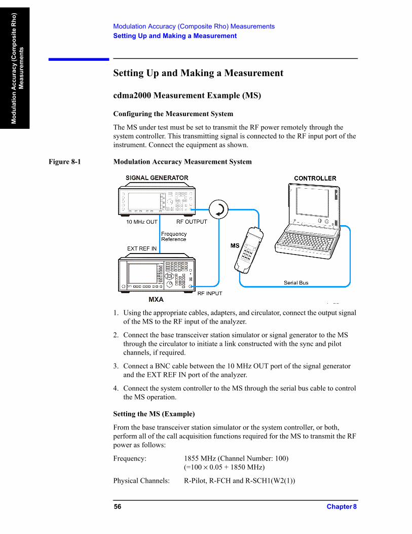
The MS under test must be set to transmit the RF power remotely through the system controller. This transmitting signal is connected to the RF input port of the instrument. Connect the equipment as shown.
Figure 8-1 Modulation Accuracy Measurement System
1. Using the appropriate cables, adapters, and circulator, connect the output signal of the MS to the RF input of the analyzer.
2. Connect the base transceiver station simulator or signal generator to the MS through the circulator to initiate a link constructed with the sync and pilot channels, if required.
3. Connect a BNC cable between the 10 MHz OUT port of the signal generator and the EXT REF IN port of the analyzer.
4. Connect the system controller to the MS through the serial bus cable to control the MS operation.
Setting the MS (Example)
From the base transceiver station simulator or the system controller, or both, perform all of the call acquisition functions required for the MS to transmit the RF power as follows:
Frequency: 1855 MHz (Channel Number: 100)(=100 × 0.05 + 1850 MHz)
Physical Channels: R-Pilot, R-FCH and R-SCH1(W2(1))
56 Chapter 8
Modulation Accuracy (Composite Rho) MeasurementsSetting Up and Making a Measurement
/t
Modulation A
ccuracy (Com
posite Rho)
Measurem
ents
Long Code Mask: 0000000000
Output Power: –20 dBm (at analyzer input)
Measurement Procedure
Step 1. Enable the cdma2000 measurements.
Press Mode, cdma2000.
Step 2. Preset the mode.
Press Mode Preset.
Step 3. Select the device to MS.
Press Mode Setup, Radio, Device to toggle the device to MS.
Step 4. Set the center frequency.
Press FREQ Channel, 1855, MHz.
Step 5. Initiate the modulation accuracy (composite Rho) measurement.
Press Meas, Mod Accuracy (Composite Rho).
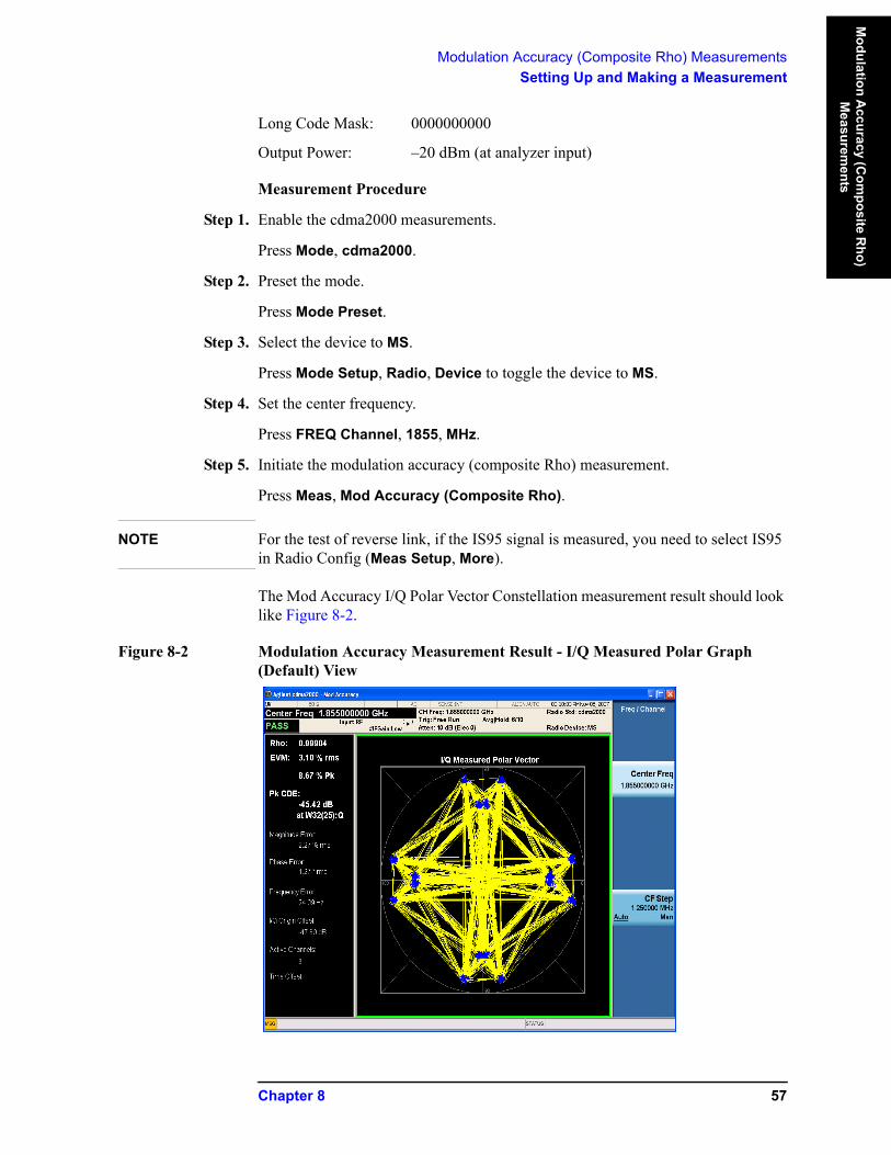
NOTE For the test of reverse link, if the IS95 signal is measured, you need to select IS95 in Radio Config (Meas Setup, More).
The Mod Accuracy I/Q Polar Vector Constellation measurement result should look like Figure 8-2.
Figure 8-2 Modulation Accuracy Measurement Result - I/Q Measured Polar Graph (Default) View
Chapter 8 57
Modulation Accuracy (Composite Rho) MeasurementsSetting Up and Making a Measurement
Mod
ulat
ion
Acc
urac
y (C
ompo
site
Rho
) M
easu
rem
ents
The modulation constellation is shown, along with summary data for Rho, EVM, Peak Code Domain Error, and phase and magnitude errors.
Step 6. Press Meas Setup to see the keys that are available to change measurement parameters from their default condition.
The PASS/FAIL in the top left corner indicates the limit test result. You can manually set the Limits (under Meas Setup menu) of RMS EVM, Peak EVM, Rho, Peak Code Domain Error, Timing Error and Phase Error. If some items do not pass the limit test, the related item will be marked with red “F”.
In the Advanced menu, you can use the EVM Result I/Q Offset key to include or exclude the I/Q origin offset in the measurement results. Also you can set the threshold relative to the channel total power to identify the active channel.
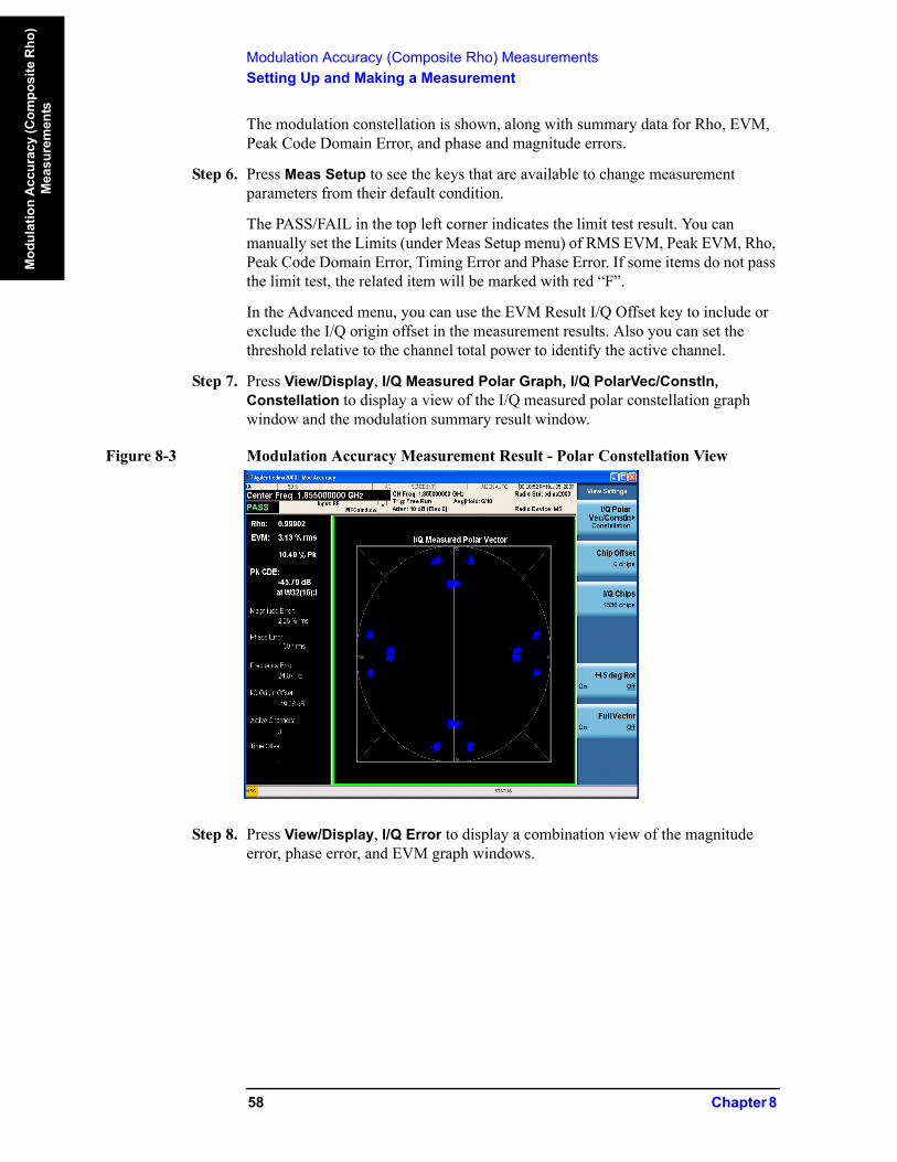
Step 7. Press View/Display, I/Q Measured Polar Graph, I/Q PolarVec/Constln, Constellation to display a view of the I/Q measured polar constellation graph window and the modulation summary result window.
Figure 8-3 Modulation Accuracy Measurement Result - Polar Constellation View
Step 8. Press View/Display, I/Q Error to display a combination view of the magnitude error, phase error, and EVM graph windows.
58 Chapter 8
Modulation Accuracy (Composite Rho) MeasurementsSetting Up and Making a Measurement
/t
Modulation A
ccuracy (Com
posite Rho)
Measurem
ents
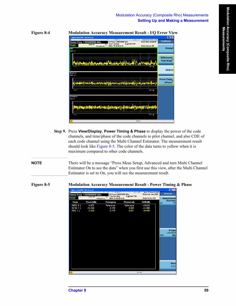
Figure 8-4 Modulation Accuracy Measurement Result - I/Q Error View
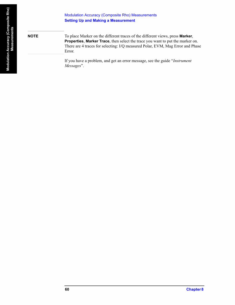
Step 9. Press View/Display, Power Timing & Phase to display the power of the code channels, and time/phase of the code channels to pilot channel, and also CDE of each code channel using the Multi Channel Estimator. The measurement result should look like Figure 8-5. The color of the data turns to yellow when it is maximum compared to other code channels.
NOTE There will be a message “Press Meas Setup, Advanced and turn Multi Channel Estimator On to see the data” when you first use this view, after the Multi Channel Estimator is set to On, you will see the measurement result.
Figure 8-5 Modulation Accuracy Measurement Result - Power Timing & Phase
Chapter 8 59
Modulation Accuracy (Composite Rho) MeasurementsSetting Up and Making a Measurement
Mod
ulat
ion
Acc
urac
y (C
ompo
site
Rho
) M
easu
rem
ents
NOTE To place Marker on the different traces of the different views, press Marker, Properties, Marker Trace, then select the trace you want to put the marker on. There are 4 traces for selecting: I/Q measured Polar, EVM, Mag Error and Phase Error.
If you have a problem, and get an error message, see the guide “Instrument Messages”.
60 Chapter 8
Modulation Accuracy (Composite Rho) MeasurementsSetting Up and Making a Measurement
/t
Modulation A
ccuracy (Com
posite Rho)
Measurem
ents
cdma2000 Measurement Example (BTS)
Configuring the Measurement System
Use the system controller to remotely control the base transceiver station (BTS) under test to transmit the RF power. The cdma2000 modulated interference signal is injected to the antenna output port of the BTS through an attenuator and circulator. The transmitting signal from the BTS is connected to the RF input port of the instrument from the circulator port. Connect the equipment as shown.
Figure 8-6 Modulation Accuracy Measurement System
1. Connect the BTS output signal to the RF input port of the analyzer through the attenuator.
2. Connect a BNC cable between the frequency reference port of the BTS and the EXT REF IN port of the analyzer.
3. Connect the system controller to the BTS through the serial bus cable.
NOTE If you want to test the Time Offset (the time from the trigger point to the PN offset), you need to connect the trigger output of the BTS to the trigger input of the analyzer.
Setting the BTS (Example)
From the BTS simulator or the system controller, or both, perform all of the call acquisition functions required for the BTS to transmit the RF power as follows:
Frequency: 1000 MHz
Physical Channels: F-Pilot, F-Paging, F-Sync with 6 F-Traffic
Scramble Code: 0
Chapter 8 61

Modulation Accuracy (Composite Rho) MeasurementsSetting Up and Making a Measurement
Mod
ulat
ion
Acc
urac
y (C
ompo
site
Rho
) M
easu
rem
ents
Output Power: –10 dBm
Measurement Procedure
Step 1. Enable the cdma2000 measurements.
Press Mode, cdma2000.
Step 2. Preset the mode.
Press Mode Preset.
Step 3. Select the device to BTS.
Press Mode Setup, Radio, Device to toggle the device to BTS.
Step 4. Set the center frequency.
Press FREQ Channel, 1000, MHz.
Step 5. Initiate the modulation accuracy (composite Rho) measurement.
Press Meas, Mod Accuracy (Composite RHO).
The Mod Accuracy I/Q Polar Vector Constellation measurement result should look like Figure 8-7.
Figure 8-7 Modulation Accuracy Measurement Result - I/Q Measured Polar Graph (Default) View
The modulation constellation is shown, along with summary data for Rho, EVM, Peak Code Domain Error, and phase and magnitude errors.
62 Chapter 8
Modulation Accuracy (Composite Rho) MeasurementsSetting Up and Making a Measurement
/t
Modulation A
ccuracy (Com
posite Rho)
Measurem
ents
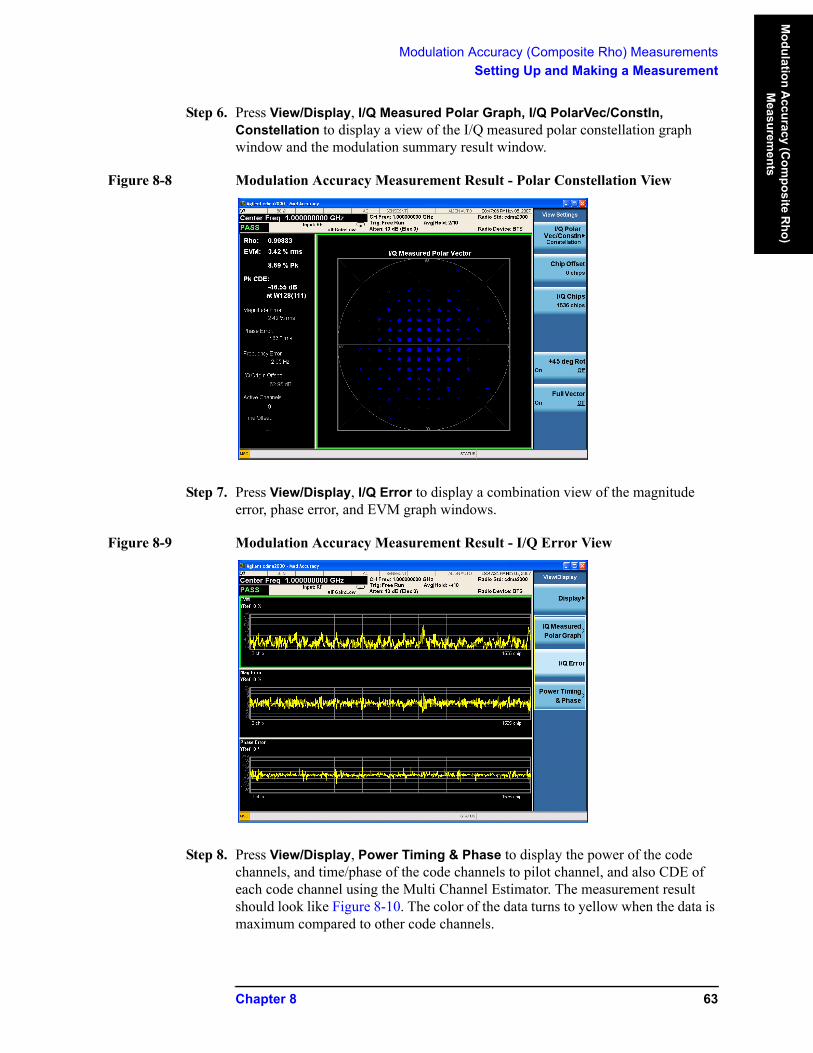
Step 6. Press View/Display, I/Q Measured Polar Graph, I/Q PolarVec/Constln, Constellation to display a view of the I/Q measured polar constellation graph window and the modulation summary result window.
Figure 8-8 Modulation Accuracy Measurement Result - Polar Constellation View
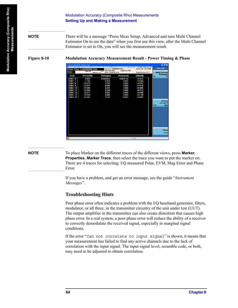
Step 7. Press View/Display, I/Q Error to display a combination view of the magnitude error, phase error, and EVM graph windows.
Figure 8-9 Modulation Accuracy Measurement Result - I/Q Error View
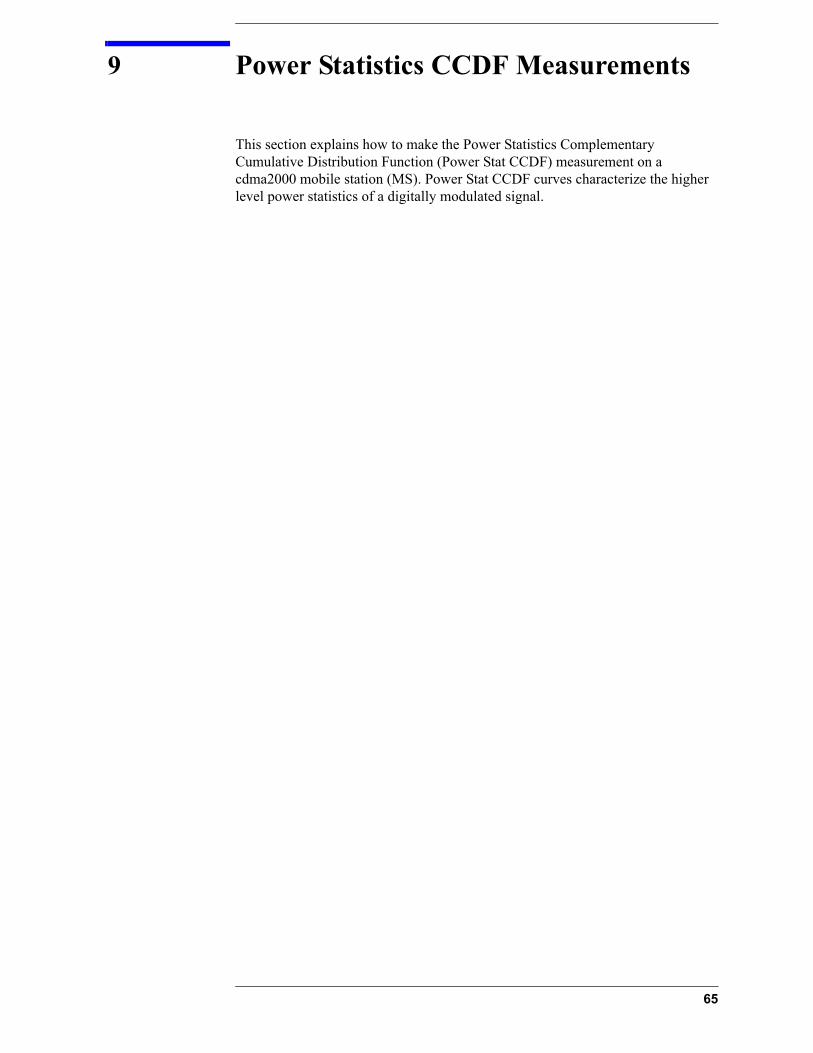
Step 8. Press View/Display, Power Timing & Phase to display the power of the code channels, and time/phase of the code channels to pilot channel, and also CDE of each code channel using the Multi Channel Estimator. The measurement result should look like Figure 8-10. The color of the data turns to yellow when the data is maximum compared to other code channels.
Chapter 8 63
Modulation Accuracy (Composite Rho) MeasurementsSetting Up and Making a Measurement
Mod
ulat
ion
Acc
urac
y (C
ompo
site
Rho
) M
easu
rem
ents
NOTE There will be a message “Press Meas Setup, Advanced and turn Multi Channel Estimator On to see the data” when you first use this view, after the Multi Channel Estimator is set to On, you will see the measurement result.
Figure 8-10 Modulation Accuracy Measurement Result - Power Timing & Phase
NOTE To place Marker on the different traces of the different views, press Marker, Properties, Marker Trace, then select the trace you want to put the marker on. There are 4 traces for selecting: I/Q measured Polar, EVM, Mag Error and Phase Error.
If you have a problem, and get an error message, see the guide “Instrument Messages”.
Troubleshooting Hints
Poor phase error often indicates a problem with the I/Q baseband generator, filters, modulator, or all three, in the transmitter circuitry of the unit under test (UUT). The output amplifier in the transmitter can also create distortion that causes high phase error. In a real system, a poor phase error will reduce the ability of a receiver to correctly demodulate the received signal, especially in marginal signal conditions.
If the error “Can not correlate to input signal” is shown, it means that your measurement has failed to find any active channels due to the lack of correlation with the input signal. The input signal level, scramble code, or both, may need to be adjusted to obtain correlation.
64 Chapter 8
9 Power Statistics CCDF Measurements
This section explains how to make the Power Statistics Complementary Cumulative Distribution Function (Power Stat CCDF) measurement on a cdma2000 mobile station (MS). Power Stat CCDF curves characterize the higher level power statistics of a digitally modulated signal.
65
Power Statistics CCDF MeasurementsSetting Up and Making a Measurement
Pow
er S
tatis
tics
CC
DF
Mea
sure
men
ts
Setting Up and Making a Measurement
Configuring the Measurement System
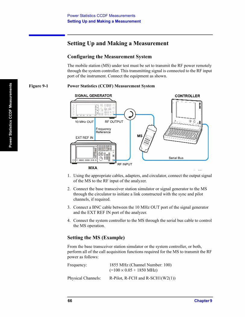
The mobile station (MS) under test must be set to transmit the RF power remotely through the system controller. This transmitting signal is connected to the RF input port of the instrument. Connect the equipment as shown.
Figure 9-1 Power Statistics (CCDF) Measurement System
1. Using the appropriate cables, adapters, and circulator, connect the output signal of the MS to the RF input of the analyzer.
2. Connect the base transceiver station simulator or signal generator to the MS through the circulator to initiate a link constructed with the sync and pilot channels, if required.
3. Connect a BNC cable between the 10 MHz OUT port of the signal generator and the EXT REF IN port of the analyzer.
4. Connect the system controller to the MS through the serial bus cable to control the MS operation.
Setting the MS (Example)
From the base transceiver station simulator or the system controller, or both, perform all of the call acquisition functions required for the MS to transmit the RF power as follows:
Frequency: 1855 MHz (Channel Number: 100)(=100 × 0.05 + 1850 MHz)
Physical Channels: R-Pilot, R-FCH and R-SCH1(W2(1))
66 Chapter 9
Power Statistics CCDF MeasurementsSetting Up and Making a Measurement
Power Statistics C
CD
F Measurem
ents
Output Power: –20 dBm (at analyzer input)
Measurement Procedure
Step 1. Enable the cdma2000 measurements.
Press Mode, cdma2000.
Step 2. Preset the mode.
Press Mode Preset.
Step 3. Select the device to MS.
Press Mode Setup, Radio, Device to toggle the device to MS.
Step 4. Set the center frequency.
Press FREQ Channel, 1855, MHz.
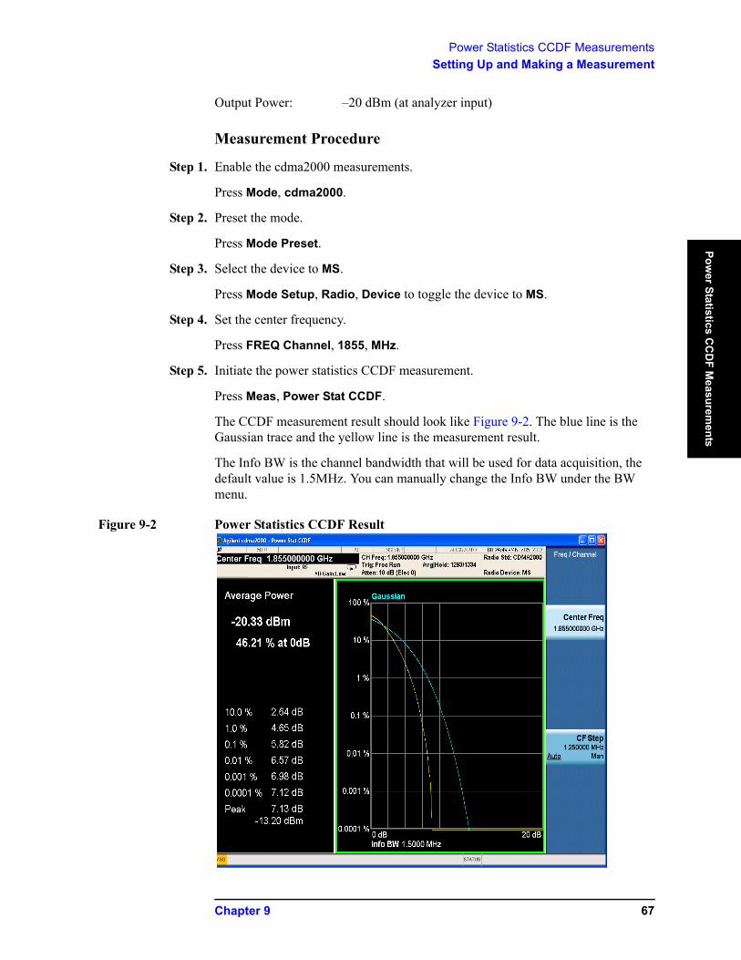
Step 5. Initiate the power statistics CCDF measurement.
Press Meas, Power Stat CCDF.
The CCDF measurement result should look like Figure 9-2. The blue line is the Gaussian trace and the yellow line is the measurement result.
The Info BW is the channel bandwidth that will be used for data acquisition, the default value is 1.5MHz. You can manually change the Info BW under the BW menu.
Figure 9-2 Power Statistics CCDF Result
Chapter 9 67
Power Statistics CCDF MeasurementsSetting Up and Making a Measurement
Pow
er S
tatis
tics
CC
DF
Mea
sure
men
ts
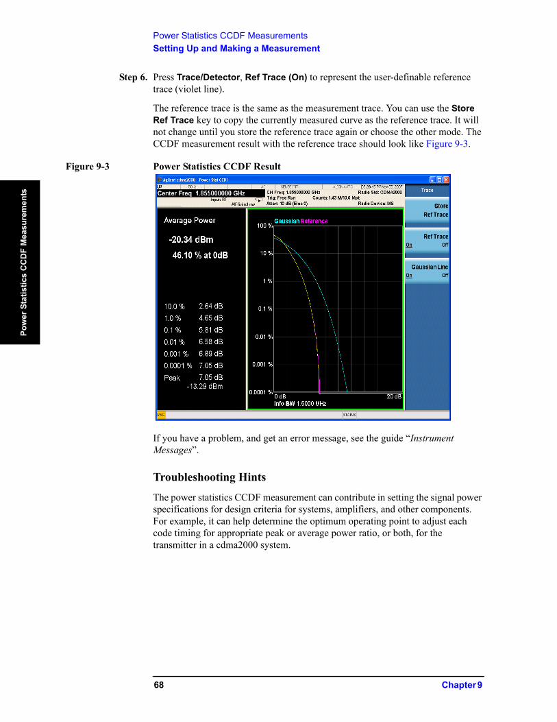
Step 6. Press Trace/Detector, Ref Trace (On) to represent the user-definable reference trace (violet line).
The reference trace is the same as the measurement trace. You can use the Store Ref Trace key to copy the currently measured curve as the reference trace. It will not change until you store the reference trace again or choose the other mode. The CCDF measurement result with the reference trace should look like Figure 9-3.
Figure 9-3 Power Statistics CCDF Result
If you have a problem, and get an error message, see the guide “Instrument Messages”.
Troubleshooting Hints
The power statistics CCDF measurement can contribute in setting the signal power specifications for design criteria for systems, amplifiers, and other components. For example, it can help determine the optimum operating point to adjust each code timing for appropriate peak or average power ratio, or both, for the transmitter in a cdma2000 system.
68 Chapter 9

10 QPSK EVM Measurements
This chapter explains how to make the QPSK error vector magnitude (EVM) measurement on a cdma2000 mobile station (MS). QPSK EVM is a measure of the phase and amplitude modulation quality relates the performance of an actual signal compared to an ideal signal as a percentage, calculated over the course of the ideal constellation.
69
QPSK EVM MeasurementsSetting Up and Making a Measurement
QPS
K E
VM M
easu
rem
ents
Setting Up and Making a Measurement
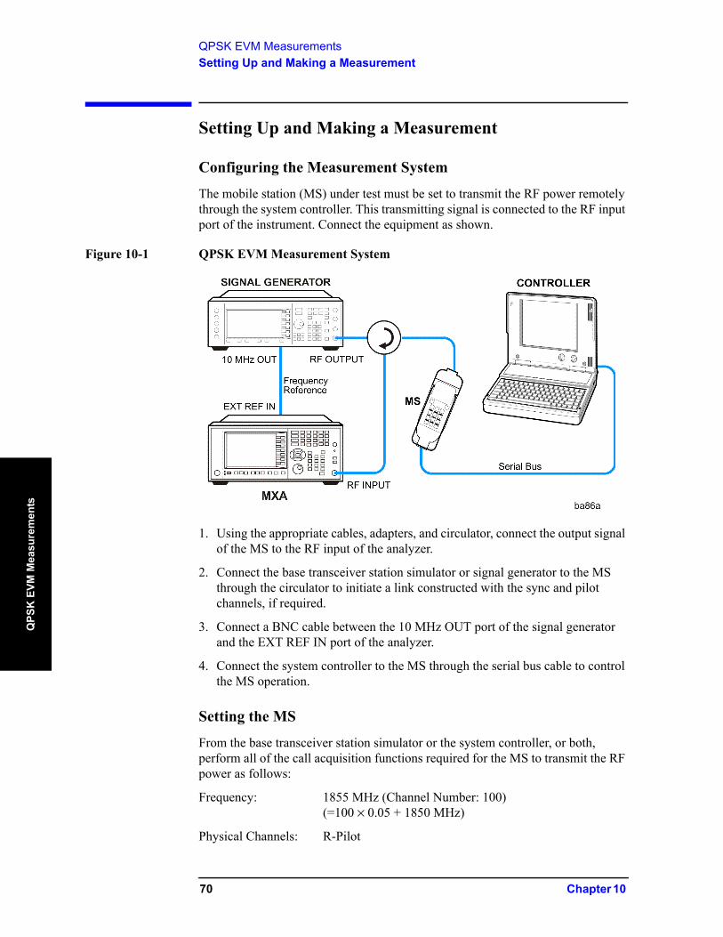
Configuring the Measurement System
The mobile station (MS) under test must be set to transmit the RF power remotely through the system controller. This transmitting signal is connected to the RF input port of the instrument. Connect the equipment as shown.
Figure 10-1 QPSK EVM Measurement System
1. Using the appropriate cables, adapters, and circulator, connect the output signal of the MS to the RF input of the analyzer.
2. Connect the base transceiver station simulator or signal generator to the MS through the circulator to initiate a link constructed with the sync and pilot channels, if required.
3. Connect a BNC cable between the 10 MHz OUT port of the signal generator and the EXT REF IN port of the analyzer.
4. Connect the system controller to the MS through the serial bus cable to control the MS operation.
Setting the MS
From the base transceiver station simulator or the system controller, or both, perform all of the call acquisition functions required for the MS to transmit the RF power as follows:
Frequency: 1855 MHz (Channel Number: 100)(=100 × 0.05 + 1850 MHz)
Physical Channels: R-Pilot
70 Chapter 10
QPSK EVM MeasurementsSetting Up and Making a Measurement
QPSK
EVM M
easurements
Scramble Code: 0
Output Power: –20 dBm (at analyzer input)
Measurement Procedure
Step 1. Enable the cdma2000 measurements.
Press Mode, cdma2000.
Step 2. Preset the mode.
Press Mode Preset.
Step 3. Select the device to MS.
Press Mode Setup, Radio, Device to toggle the device to MS.
Step 4. Set the center frequency.
Press FREQ Channel, 1855, MHz.
Step 5. Initiate the QPSK EVM measurement.
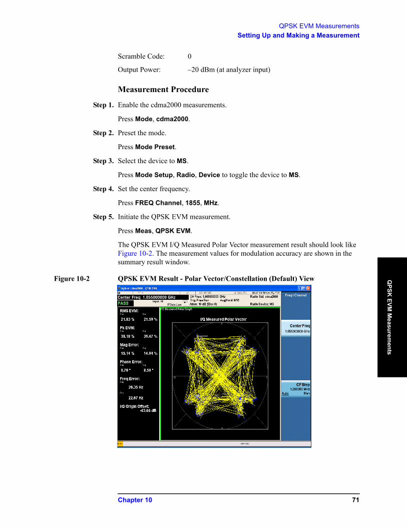
Press Meas, QPSK EVM.
The QPSK EVM I/Q Measured Polar Vector measurement result should look like Figure 10-2. The measurement values for modulation accuracy are shown in the summary result window.
Figure 10-2 QPSK EVM Result - Polar Vector/Constellation (Default) View
Chapter 10 71
QPSK EVM MeasurementsSetting Up and Making a Measurement
QPS
K E
VM M
easu
rem
ents
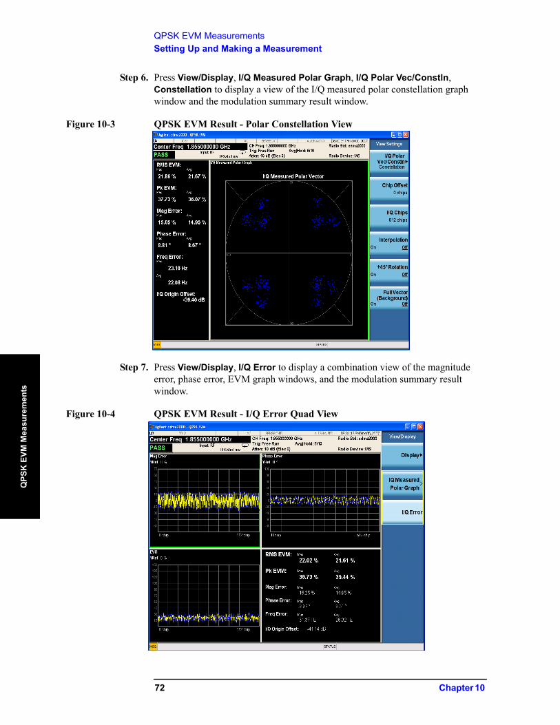
Step 6. Press View/Display, I/Q Measured Polar Graph, I/Q Polar Vec/Constln, Constellation to display a view of the I/Q measured polar constellation graph window and the modulation summary result window.
Figure 10-3 QPSK EVM Result - Polar Constellation View
Step 7. Press View/Display, I/Q Error to display a combination view of the magnitude error, phase error, EVM graph windows, and the modulation summary result window.
Figure 10-4 QPSK EVM Result - I/Q Error Quad View
72 Chapter 10
QPSK EVM MeasurementsSetting Up and Making a Measurement
QPSK
EVM M
easurements
Step 8. Press Meas Setup to see the keys that are available to change measurement parameters from their default condition.
The PASS/FAIL in the top left corner indicates the limit test result. You can manually set the Limits (under Meas Setup menu) of RMS EVM and Freq Error. If some items do not pass the limit test, the related item will be marked with red “F”.
In the Advanced menu, you can use the EVM Result I/Q Offset key to include or exclude the I/Q origin offset in the measurement results.
NOTE In the View/Display menu, the Display key and the IQ Measured Polar Graph key has an arrow in the right middle of the button. If the arrow is hollow, you need to press the key to select the view and the hollow arrow turns solid, If you press the key again, the view settings about this view will be displayed.
If you have a problem, and get an error message, see the guide “Instrument Messages”.
Troubleshooting Hints
Poor phase error indicates a problem with the I/Q baseband generator, filters, or modulator, or all, in the transmitter circuitry of the unit under test (UUT). The output amplifier in the transmitter can also create distortion that causes unacceptably high phase error. In a real system, a poor phase error will reduce the ability of a receiver to correctly demodulate the received signal, especially in marginal signal conditions.
Chapter 10 73
QPSK EVM MeasurementsSetting Up and Making a Measurement
QPS
K E
VM M
easu
rem
ents
74 Chapter 10
11 Monitor Spectrum Measurements
This chapter explains how to make a Monitor Spectrum measurement on a cdma2000 MS (Mobile Station). Monitor Spectrum measurements show a spectrum domain display of the cdma2000 signal.
This example shows a MS under test set up to transmit RF power, and controlled remotely by a system controller. The transmitting signal is connected to the RF input port of the instrument. Connect the equipment as shown.
75
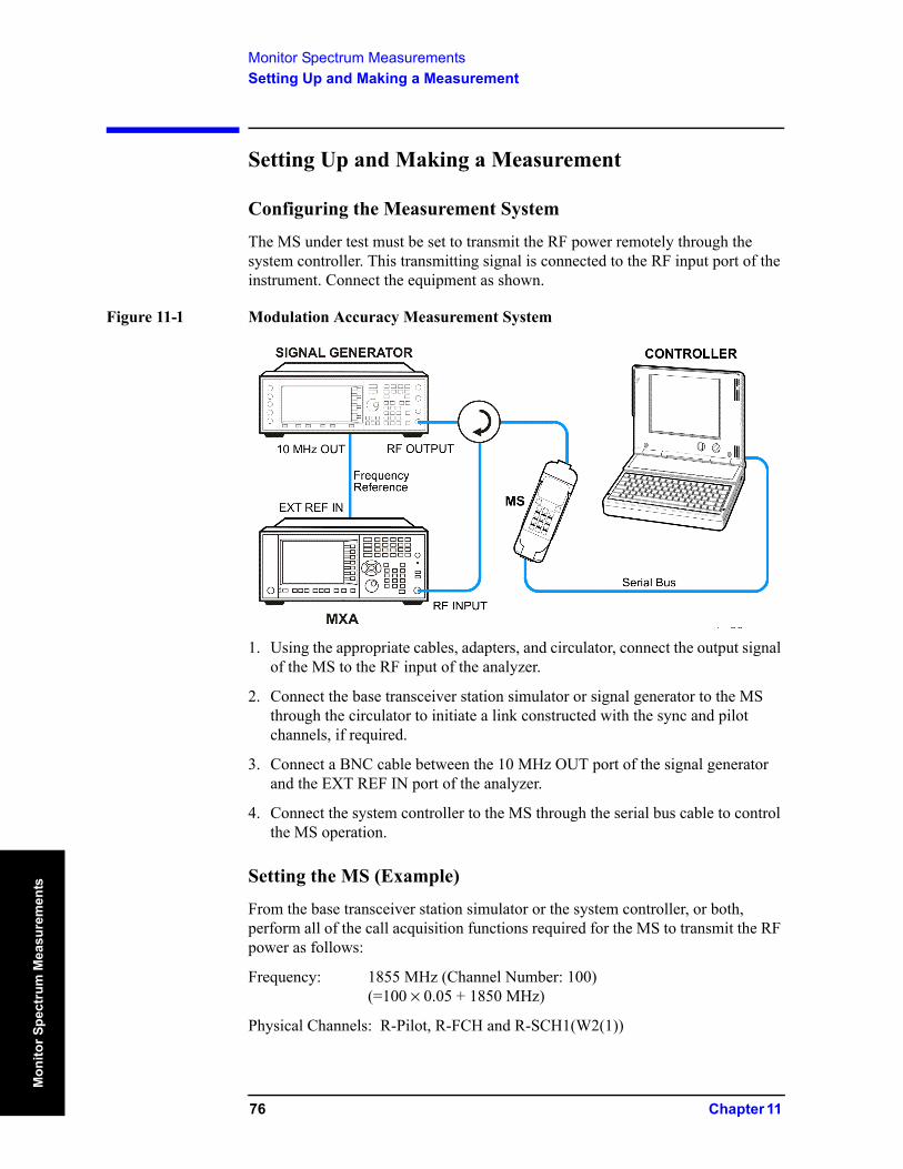
Monitor Spectrum MeasurementsSetting Up and Making a Measurement
Mon
itor S
pect
rum
Mea
sure
men
ts
Setting Up and Making a Measurement
Configuring the Measurement System
The MS under test must be set to transmit the RF power remotely through the system controller. This transmitting signal is connected to the RF input port of the instrument. Connect the equipment as shown.
Figure 11-1 Modulation Accuracy Measurement System
1. Using the appropriate cables, adapters, and circulator, connect the output signal of the MS to the RF input of the analyzer.
2. Connect the base transceiver station simulator or signal generator to the MS through the circulator to initiate a link constructed with the sync and pilot channels, if required.
3. Connect a BNC cable between the 10 MHz OUT port of the signal generator and the EXT REF IN port of the analyzer.
4. Connect the system controller to the MS through the serial bus cable to control the MS operation.
Setting the MS (Example)
From the base transceiver station simulator or the system controller, or both, perform all of the call acquisition functions required for the MS to transmit the RF power as follows:
Frequency: 1855 MHz (Channel Number: 100)(=100 × 0.05 + 1850 MHz)
Physical Channels: R-Pilot, R-FCH and R-SCH1(W2(1))
76 Chapter 11
Monitor Spectrum MeasurementsSetting Up and Making a Measurement
Monitor Spectrum
Measurem
ent
Output Power: –20 dBm (at analyzer input)
Measurement Procedure
Step 1. Enable the cdma2000 Mode:
Press Mode,cdma2000.
Step 2. Preset the analyzer mode:
Press Mode Preset.
Step 3. Set the measurement center frequency:
Press FREQ Channel, enter a numerical frequency using the front-panel keypad, and select a units key, such as MHz.
Step 4. Set the measurement span frequency:
Press SPAN X Scale, enter a numerical span using the front-panel keypad, and select a units key, such as MHz.
Step 5. Initiate the measurement:
Press Meas, Monitor Spectrum.
The default display shows the Current (yellow trace) data. To make viewing the display easier, you can view either the Current trace or Average separately.
• Press Trace/Detector, Select Trace and select the trace(s) desired for display, then toggle Display to Show. Then press Update to On to see the timely update trace.
Chapter 11 77
s
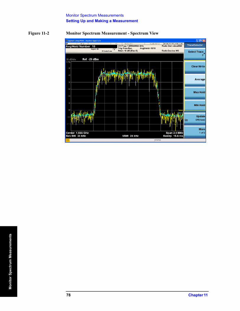
Monitor Spectrum MeasurementsSetting Up and Making a Measurement
Mon
itor S
pect
rum
Mea
sure
men
ts
Figure 11-2 Monitor Spectrum Measurement - Spectrum View
78 Chapter 11

12 IQ Waveform (Time Domain) Measurements
This chapter explains how to make a waveform (time domain) measurement on a cdma2000 mobile station. The measurement of I and Q modulated waveforms in the time domain disclose the voltages which comprise the complex modulated waveform of a digital signal.79

IQ Waveform (Time Domain) MeasurementsSetting Up and Making Measurements
IQ W
avef
orm
(Tim
e D
omai
n)
Mea
sure
men
ts
Setting Up and Making Measurements
Configuring the Measurement System
The MS under test must be set to transmit the RF power remotely through the system controller. This transmitting signal is connected to the RF input port of the instrument. Connect the equipment as shown.
Figure 12-1 Waveform Measurement System
1. Using the appropriate cables, adapters, and circulator, connect the output signal from the MS to the RF input port of the analyzer.
2. Connect the base transceiver station simulator or signal generator to the MS through the circulator to initiate a link constructed with the sync and pilot channels, if required.
3. Connect a BNC cable between the 10 MHz OUT port of the signal generator and the EXT REF IN port of the analyzer.
4. Connect the system controller to the MS through the serial bus cable to control the MS operation.
Setting the MS (Example)
From the base transceiver station simulator or the system controller, or both, perform all of the call acquisition functions required for the MS to transmit the RF power as follows:
Frequency: 1855 MHz (Channel Number: 100)(=100 × 0.05 + 1850 MHz)
Output Power: -20 dBm (at analyzer input)
80 Chapter 12

IQ Waveform (Time Domain) MeasurementsSetting Up and Making Measurements
IQ W
aveform (Tim
e Dom
ain) M
easurements
Measurement Procedure
Step 1. Set the analyzer to the appropriate mode and enable the Mode measurements:
Press Mode, cdma2000.
Step 2. Preset the analyzer mode:
Press Mode Preset.
Step 3. Set the measurement center frequency:
Press FREQ Channel, enter a numerical frequency using the front-panel keypad, and select a units key, for example MHz.
Step 4. Set the measurement span frequency:
Press SPAN X Scale key, enter a numerical span using the front-panel keypad, and select a units key, for example MHz.
Step 5. Initiate the IQ Waveform measurement:
Press Meas, IQ Waveform.
The default display shows the RF Envelope with the current data. The measured values for the mean power and peak-to-mean power are shown in the text window.
Figure 12-2 Waveform Measurement - RF Envelope (Default View)
Step 6. Select the view.
Press View/Display, IQ Waveform.
• The IQ Waveform window provides a view of the I (yellow trace) and Q (blue trace) waveforms on the same graph in terms of voltage versus time in linear
Chapter 12 81
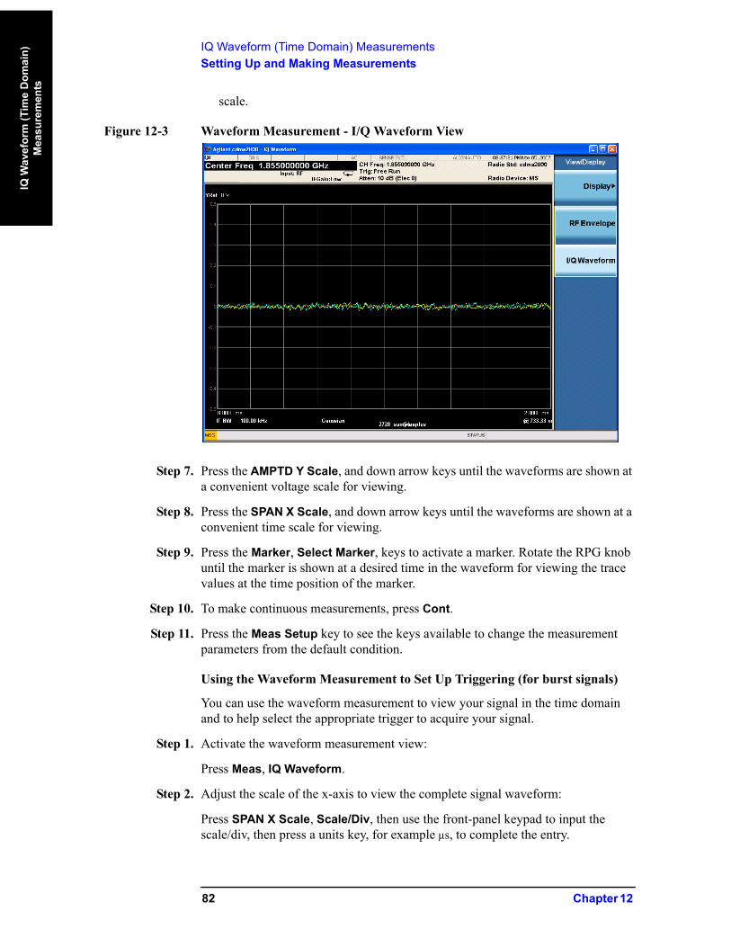
IQ Waveform (Time Domain) MeasurementsSetting Up and Making Measurements
IQ W
avef
orm
(Tim
e D
omai
n)
Mea
sure
men
ts
scale.
Figure 12-3 Waveform Measurement - I/Q Waveform View
Step 7. Press the AMPTD Y Scale, and down arrow keys until the waveforms are shown at a convenient voltage scale for viewing.
Step 8. Press the SPAN X Scale, and down arrow keys until the waveforms are shown at a convenient time scale for viewing.
Step 9. Press the Marker, Select Marker, keys to activate a marker. Rotate the RPG knob until the marker is shown at a desired time in the waveform for viewing the trace values at the time position of the marker.
Step 10. To make continuous measurements, press Cont.
Step 11. Press the Meas Setup key to see the keys available to change the measurement parameters from the default condition.
Using the Waveform Measurement to Set Up Triggering (for burst signals)
You can use the waveform measurement to view your signal in the time domain and to help select the appropriate trigger to acquire your signal.
Step 1. Activate the waveform measurement view:
Press Meas, IQ Waveform.
Step 2. Adjust the scale of the x-axis to view the complete signal waveform:
Press SPAN X Scale, Scale/Div, then use the front-panel keypad to input the scale/div, then press a units key, for example µs, to complete the entry.
82 Chapter 12

IQ Waveform (Time Domain) MeasurementsSetting Up and Making Measurements
IQ W
aveform (Tim
e Dom
ain) M
easurements
Step 3. Select a trigger source (free run is the default setting):
Press Trigger, then select one of the available trigger sources. You can also setup trigger holdoff and auto trigger timing.
Chapter 12 83

IQ Waveform (Time Domain) MeasurementsSetting Up and Making Measurements
IQ W
avef
orm
(Tim
e D
omai
n)
Mea
sure
men
ts
84 Chapter 12
Concepts
13 Concepts
This chapter provides details about the cdma2000 communications systems, and explains how the various measurements are performed by the instrument. Suggestions for optimizing and troubleshooting your setup are provided, along with a list of related Agilent documents that are referenced for further information.
85
ConceptsWhat Is the cdma2000 Communication System?
Con
cept
s
What Is the cdma2000 Communication System?
Introduction
Code Division Multiple Access 2000 (cdma2000) is a wideband CDMA standard that has been adopted by 3GPP2. It provides a wideband air interface for third generation global wireless communications systems. cdma2000 is a derivative of the IS-95-B CDMA system, also known as cdmaOne, and provides an upgrade path to support IMT-2000. This section will present the basics of cdma2000 as it differs from IS-95, and will assume the reader has some familiarity with IS-95 technology.
cdma2000 is defined in the following Telecommunications Industry Association (TIA) and Electronics Industry Alliance (EIA) document: TIA/EIA/IS-2000-1 through TIA/EIA/IS-2000-6.
cdma2000 relies on the Global Positioning System (GPS) for intercell synchronization. Both reverse and forward transmitter power controls are implemented with 1.25 ms intervals. cdma2000 is a direct sequence spread-spectrum digital communications technique that supports wider RF bandwidths from 1.25 to 15 MHz. The main advantages of cdma2000 over other types of digital communication schemes are:
• greater capacity• immunity to signal loss and degradation due to high-level broadband
interference, multipath, and fading• strict minimization of power consumption for mobile stations by both base
station and mobile controls• support for variable data rates; up to 144 kbits/second for mobile (vehicular)
data rate, up to 384 kbits/second for portable (pedestrian) data rate, and up to 2 Mbits/second for fixed installations
• increased security
cdma2000 uses correlative codes to distinguish one user from another. Frequency division is still used, as is done with Frequency Division Multiple Access (FDMA) and Time Division Multiple Access (TDMA), but in a much larger bandwidth such as 1.25 MHz or greater. cdma2000 realizes increased capacity from 1:1 frequency reuse and sectored cells. The capacity limit is soft. That is, capacity can be increased with some degradation of the error rate or voice quality.
In cdma2000, a single user's channel consists of a specific frequency combined with a unique Walsh code channel. Correlative Walsh codes allow each user to operate in the presence of substantial interference. The interference is the sum of all other users on the same cdma2000 frequency, both from within and outside of the home cell, and from delayed versions of these signals. It also includes the usual thermal noise and atmospheric disturbances. Delayed signals caused by multipath are separately received and combined in cdma2000. One of the major differences in access is that any cdma2000 frequency can be used in all sectors of all cells. This is possible because cdma2000 is designed to decode the proper signal in the
86 Chapter 13
ConceptsWhat Is the cdma2000 Communication System?
Concepts
presence of high interference.
Also, cdma2000 offers a number of RF structures to accommodate almost any conceivable application. These options include direct spreading to support those applications where clear spectrum is available, and multi-carrier arrangements using 1.25 MHz wide channels to allow overlays with TIA/EIA-95-B systems.
Spreading Rate
Spreading rate (SR) defines the final spread chip rate in terms of 1.2288 Mcps (Mega Chips Per Second). The two spreading rates are SR1 and SR3. An SR1 signal has a chip rate of 1.2288 Mcps and occupies the same bandwidth as cdmaOne signals. The SR1 system doubles the system capacity, therefore, it can be considered an improved cdmaOne system.
There are two main differences between cdmaOne and cdma2000. The first difference is fast power control and quadrature phase shift keying (QPSK) modulation rather than dual binary phase shift keying (BPSK) in the forward link. The second difference is the presence of a pilot signal, to allow coherent demodulation, and hybrid phase shift keying (HPSK) spreading in the reverse link.
An SR3 cdma2000 signal has a rate of 3.6864 Mcps (3 x 1.2288 Mcps) and occupies three times the bandwidth of cdmaOne. Originally, the SR3 system appeared to be viable. Upon further investigation the SR3 cdma2000 system was determined not to be viable and is no longer receiving any commercial attention at this time. Therefore, we will not cover SR3 in this section.
Radio Configuration
Radio configuration (RC) defines the physical channel configuration based upon a specific channel data rate. Each RC specifies a set of data rates based on either 9.6 or 14.4 kbps bit streams, the two existing data rates supported for cdmaOne. Each RC also specifies the spreading rate (either SR1 or SR3) and the physical coding. Currently there are nine radio configurations defined in the cdma2000 system for the forward link and six for the reverse link. Examples include:
• RC1 is the backwards-compatible mode of cdmaOne for 9600-bps voice traffic. It includes 9.6, 4.8, 2.4, and 1.2 kbps data rates and operates at SR1. It does not use any of the cdma2000 coding improvements.
• RC3 is a cdma2000-specific configuration based on 9.6 kbps that also supports 4.8, 2.7, and 1.5 kbps for voice, while supporting data at 19.2, 38.4, 76.8, and 153.6 kbps and operates at SR1. Each base transceiver station (BTS) or MS must be capable of transmitting using different RCs at the same SR. Refer to [2] for detailed information on the different RCs.
Forward Link Air Interface
The forward link air interface for a cdma2000 SR1 channel is very similar to that of cdmaOne. In order to preserve compatibility, cdma2000 uses the same structure as cdmaOne for the forward pilot (F-Pilot), forward sync (F-Sync), and forward
Chapter 13 87
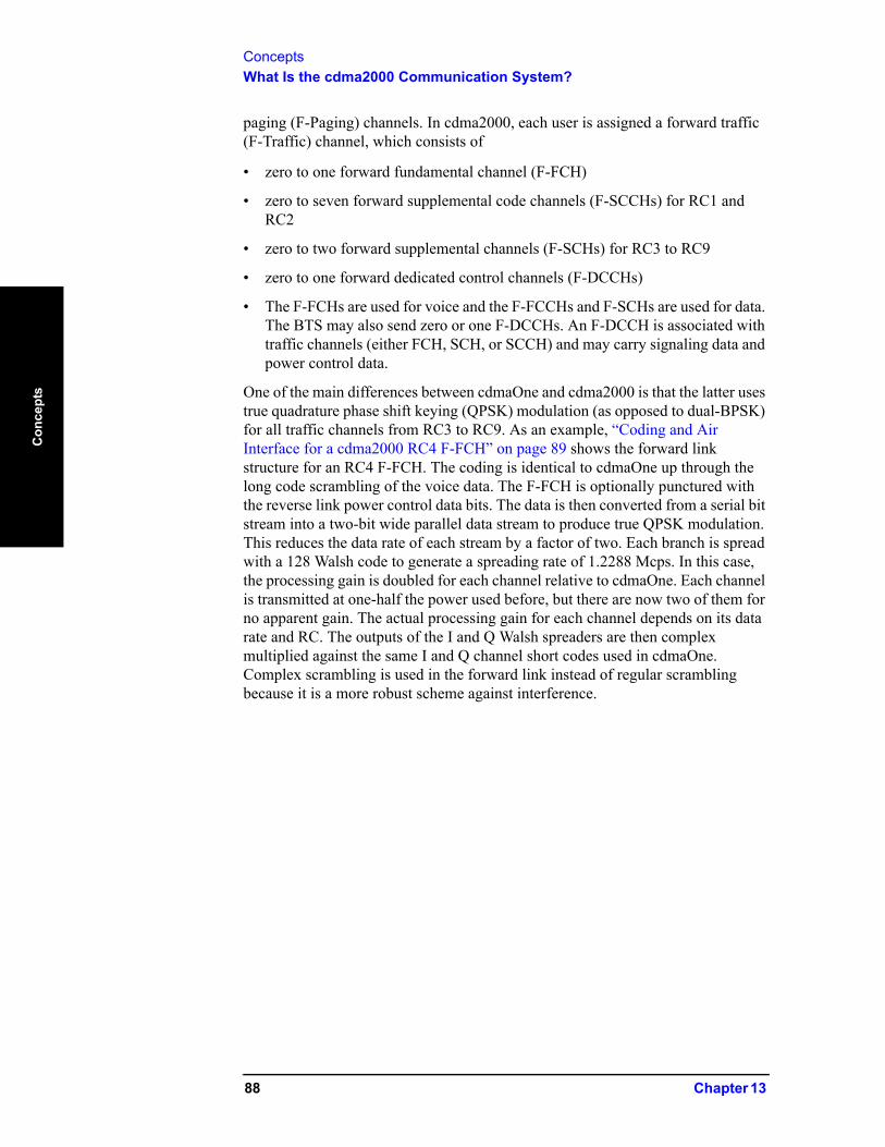
ConceptsWhat Is the cdma2000 Communication System?
Con
cept
s
paging (F-Paging) channels. In cdma2000, each user is assigned a forward traffic (F-Traffic) channel, which consists of
• zero to one forward fundamental channel (F-FCH)
• zero to seven forward supplemental code channels (F-SCCHs) for RC1 and RC2
• zero to two forward supplemental channels (F-SCHs) for RC3 to RC9
• zero to one forward dedicated control channels (F-DCCHs)
• The F-FCHs are used for voice and the F-FCCHs and F-SCHs are used for data. The BTS may also send zero or one F-DCCHs. An F-DCCH is associated with traffic channels (either FCH, SCH, or SCCH) and may carry signaling data and power control data.
One of the main differences between cdmaOne and cdma2000 is that the latter uses true quadrature phase shift keying (QPSK) modulation (as opposed to dual-BPSK) for all traffic channels from RC3 to RC9. As an example, “Coding and Air Interface for a cdma2000 RC4 F-FCH” on page 89 shows the forward link structure for an RC4 F-FCH. The coding is identical to cdmaOne up through the long code scrambling of the voice data. The F-FCH is optionally punctured with the reverse link power control data bits. The data is then converted from a serial bit stream into a two-bit wide parallel data stream to produce true QPSK modulation. This reduces the data rate of each stream by a factor of two. Each branch is spread with a 128 Walsh code to generate a spreading rate of 1.2288 Mcps. In this case, the processing gain is doubled for each channel relative to cdmaOne. Each channel is transmitted at one-half the power used before, but there are now two of them for no apparent gain. The actual processing gain for each channel depends on its data rate and RC. The outputs of the I and Q Walsh spreaders are then complex multiplied against the same I and Q channel short codes used in cdmaOne. Complex scrambling is used in the forward link instead of regular scrambling because it is a more robust scheme against interference.
88 Chapter 13

ConceptsWhat Is the cdma2000 Communication System?
Concepts
Figure 13-1 Coding and Air Interface for a cdma2000 RC4 F-FCH
Reverse link air interface — HPSK
The cdma2000 reverse link is very different from cdmaOne. The MS can transmit more than one code channel to accommodate the high data rates. The minimum configuration consists of a reverse pilot (R-Pilot) channel to allow the BTS to perform synchronous detection and a reverse fundamental channel (R-FCH) for voice. Additional channels, such as the reverse supplemental channels (R-SCHs) and the reverse dedicated control channel (R-DCCH) can be used to send data or signaling information, respectively.
The different channels are assigned to either the I or Q path. For example, for RC3 to RC6, the R-Pilot is assigned to I and R-FCH is assigned to Q (see Figure 13-2 on page 90).
1/ 4 Rate conv.encoder
Interleaver
Long codedecimator
Walsh 64generator
1228.8 kcps
1228.8 kcps
∑
∑
I
Q
1228.8 kcps
1228.8 kcps
Complex scrambling
1228.8 kcps
1228.8 kcps
+
–
+
+
I short code
Q short codeFIR
FIRI
Q
S-P
19.2 ksps
19.2 ksps
I
Q
P.C.
Gain
P.C.dec
P.C.bits
800 bps
800 bps
GainUser longcode mask
Long codegenerator
Add CRC and tail bits
Full ratedata bits
Puncturetiming38.4 ksps
9.6 ksps
38.4 ksps
8.6 ksps
38.4 ksps
38.4 ksps
1228.8 kcps
Decimate byWalsh length/ 2
Powercontrol
puncture
Orthogonalspreading
OptionalCan be carried by F-DCCH
I
Q1228.8 kcps
1228.8 kcps
Chapter 13 89
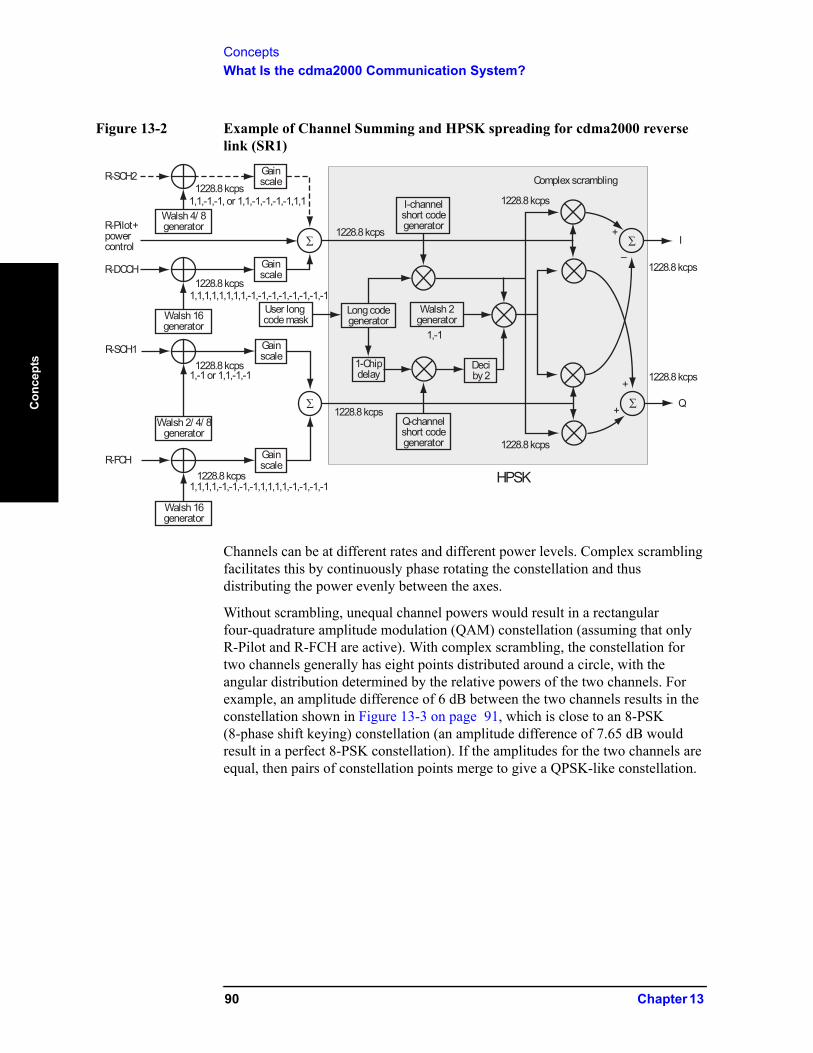
ConceptsWhat Is the cdma2000 Communication System?
Con
cept
s
Figure 13-2 Example of Channel Summing and HPSK spreading for cdma2000 reverse link (SR1)
Channels can be at different rates and different power levels. Complex scrambling facilitates this by continuously phase rotating the constellation and thus distributing the power evenly between the axes.
Without scrambling, unequal channel powers would result in a rectangular four-quadrature amplitude modulation (QAM) constellation (assuming that only R-Pilot and R-FCH are active). With complex scrambling, the constellation for two channels generally has eight points distributed around a circle, with the angular distribution determined by the relative powers of the two channels. For example, an amplitude difference of 6 dB between the two channels results in the constellation shown in Figure 13-3 on page 91, which is close to an 8-PSK (8-phase shift keying) constellation (an amplitude difference of 7.65 dB would result in a perfect 8-PSK constellation). If the amplitudes for the two channels are equal, then pairs of constellation points merge to give a QPSK-like constellation.
1,1,1,1,1,1,1,1,-1,-1,-1,-1,-1,-1,-1,-1
R-SCH2
Walsh 4/ 8generator
Q-channelshort codegenerator
1228.8 kcps
User long code mask
Gainscale
R-DCCH
Walsh 16generator
Gainscale
R-Pilot+powercontrol
1228.8 kcps
∑
R-SCH1
Walsh 2/ 4/ 8generator
1228.8 kcps
Gainscale
R-FCH
Walsh 16generator
Gainscale
1228.8 kcps
∑
Long codegenerator
Walsh 2generator
1-Chipdelay
Deciby 2
I-channelshort codegenerator
1228.8 kcps
1228.8 kcps∑
∑
I
Q
1228.8 kcps
1228.8 kcps
Complex scrambling
1228.8 kcps
1228.8 kcps
+
–
+
+
1,1,-1,-1, or 1,1,-1,-1,-1,-1,1,1
1,-1 or 1,1,-1,-1
1,1,1,1,-1,-1,-1,-1,1,1,1,1,-1,-1,-1,-1
1,-1
HPSK
90 Chapter 13
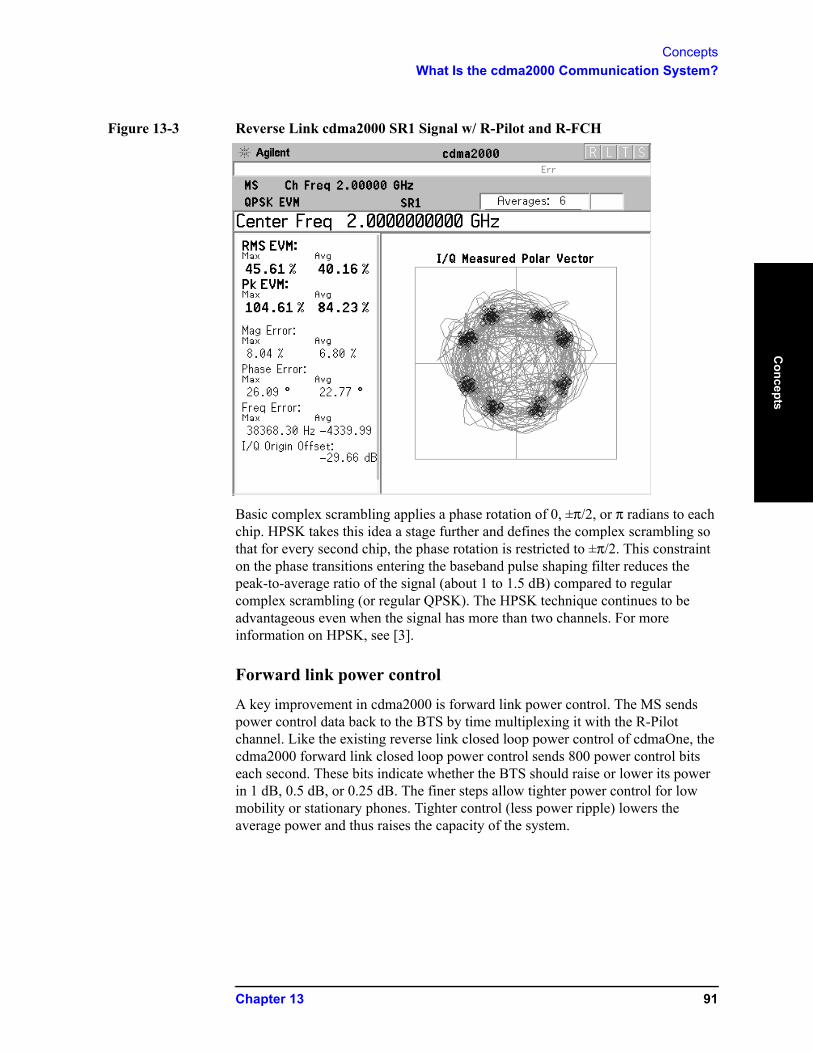
ConceptsWhat Is the cdma2000 Communication System?
Concepts
Figure 13-3 Reverse Link cdma2000 SR1 Signal w/ R-Pilot and R-FCH
Basic complex scrambling applies a phase rotation of 0, ±π/2, or π radians to each chip. HPSK takes this idea a stage further and defines the complex scrambling so that for every second chip, the phase rotation is restricted to ±π/2. This constraint on the phase transitions entering the baseband pulse shaping filter reduces the peak-to-average ratio of the signal (about 1 to 1.5 dB) compared to regular complex scrambling (or regular QPSK). The HPSK technique continues to be advantageous even when the signal has more than two channels. For more information on HPSK, see [3].
Forward link power control
A key improvement in cdma2000 is forward link power control. The MS sends power control data back to the BTS by time multiplexing it with the R-Pilot channel. Like the existing reverse link closed loop power control of cdmaOne, the cdma2000 forward link closed loop power control sends 800 power control bits each second. These bits indicate whether the BTS should raise or lower its power in 1 dB, 0.5 dB, or 0.25 dB. The finer steps allow tighter power control for low mobility or stationary phones. Tighter control (less power ripple) lowers the average power and thus raises the capacity of the system.
Chapter 13 91
ConceptsWhat Is the cdma2000 Communication System?
Con
cept
s
Differences between cdma2000 and W-CDMA
The Third-Generation Partnership Project (3GPP) W-CDMA is the other main wideband CDMA technology competing for the 3G cellular market. There has been much discussion about the need to harmonize W-CDMA and cdma2000 in an attempt to facilitate global use of 3G phones. However, even though both systems are based on a similar CDMA technology, they are significantly different. The main differences are:
• spreading rate - (3.84 Mcps for W-CDMA versus 1.2288 Mcps for cdma2000 SR1)
• synchronization and BTS identification methodology - W-CDMA does not use GPS, or Global Positioning System. For information on-CDMA user equipment (UE)1 design and test issues, refer to [4].
1. W-CDMA specifications use the term UE to refer to mobile phones or other computing devices that provide wireless access to the W-CDMA system.
92 Chapter 13
ConceptsAdjacent Channel Power (ACP) Measurement Concepts
Concepts
Adjacent Channel Power (ACP) Measurement Concepts
Purpose
Adjacent Channel Power (ACP), as it applies to cdma2000, is the power contained in a specified frequency channel bandwidth relative to the total carrier power. It may also be expressed as a ratio of power spectral densities between the carrier and the specified offset frequency band.
As a composite measurement of out-of-channel emissions, ACP combines both in-band and out-of-band specifications to provide useful figures-of-merit for spectral regrowth and emissions produced by components and circuit blocks without the rigor of performing a full spectrum emissions mask measurement.
To maintain a quality call by avoiding channel interference, it is important to measure and reduce any adjacent channel leakage power transmitted from a mobile phone. The characteristics of adjacent channel leakage power are mainly determined by the transmitter design, particularly the low-pass filter.
Measurement Method
This ACP measurement analyzes the total power levels within the defined carrier bandwidth and at given frequency offsets on both sides of the carrier frequency. This measurement requires the user to specify measurement bandwidths of the carrier channel and each of the offset frequency pairs up to 5. Each pair may be defined with unique measurement bandwidths.
For Meas Method of RBW, it uses an appropriate RBW and capture all of the power in the carrier channel and the offsets. For Meas Method of integration bandwidth (IBW), the channel integration bandwidth is analyzed using the user defined resolution bandwidth (RBW), which is much narrower than the channel bandwidth. The measurement computes an average power of the channel over a specified number of data acquisitions, automatically compensating for resolution bandwidth and noise bandwidth.
If Total Pwr Ref is selected as the measurement type, the results are displayed as relative power in dBc and as absolute power in dBm. If PSD Ref (Power Spectral Density Reference) is selected, the results are displayed as relative power in dB, and as absolute power in dBm/Hz.
Recommended Offset Frequencies and Reference Bandwidths
While the user sets the specific offsets and reference bandwidths, the radio specifications recommend some common setups as shown in the following table. The offset frequency is titled as Offset to Edge in the measurement result window. For example, if the measurement bandwidth is set to 30 kHz, the first offset center frequency can be 765 kHz and the offset to edge frequency can be 750 kHz.
Chapter 13 93
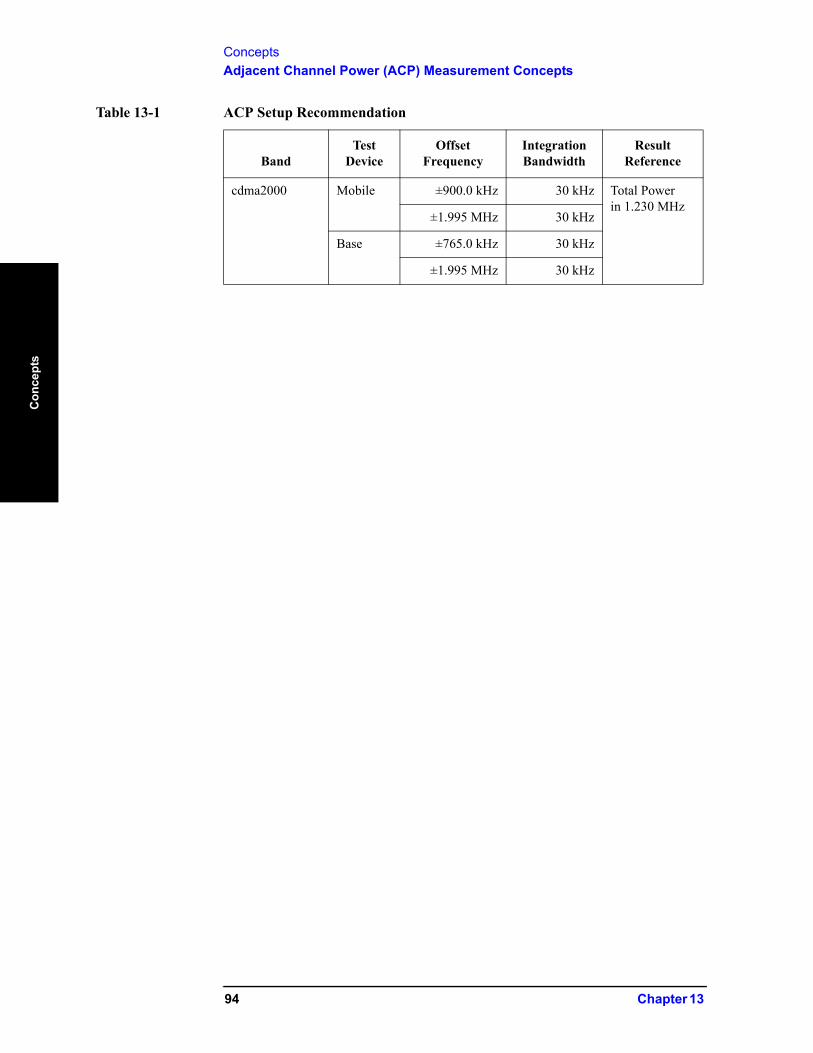
ConceptsAdjacent Channel Power (ACP) Measurement Concepts
Con
cept
s
Table 13-1 ACP Setup Recommendation
BandTest
DeviceOffset
FrequencyIntegration Bandwidth
Result Reference
cdma2000 Mobile ±900.0 kHz 30 kHz Total Powerin 1.230 MHz
±1.995 MHz 30 kHz
Base ±765.0 kHz 30 kHz
±1.995 MHz 30 kHz
94 Chapter 13
ConceptsChannel Power Measurement Concepts
Concepts
Channel Power Measurement Concepts
Purpose
The Channel Power measurement is a common test used in the wireless industry to measure the total transmitted power of a radio within a defined frequency channel. This procedure measures the total power within the defined channel for cdma2000. This measurement is applied to design, characterize, evaluate, and verify transmitters and their components or devices for base stations and mobile stations.
Measurement Method
The Channel Power measurement reports the total transmitted power within the channel bandwidth, 1.23000 MHz for the cdma2000 mode. It takes a sweep and the measurement acquires power in the carrier channel.
The measurement uses the frequency sweep mode, you can change the RBW and VBW setings.
To improve repeatability, you can increase the number of averages. The channel power graph is shown in the graph window, while the absolute channel power in dBm and the mean power spectral density in dBm/Hz are shown in the text window.
Chapter 13 95
ConceptsCode Domain Measurement Concepts
Con
cept
s
Code Domain Measurement Concepts
Purpose
Since the code domain measurements despread and descramble the cdma2000 signal into its physical channels, the number of active channels of various symbol rates (which are denoted by widths) can be observed. The width of the channel is inversely proportional to the Walsh code length in number of bits. In the code domain, there is a fixed amount of code space for a given chip rate. Therefore, by using the different Walsh codes, the system can dynamically allocate the code space for lower rate voice users versus high speed data users.
This code domain power composite view provides information about the in-channel characteristics of the cdma2000 signal. It informs the user of the active channels with their individual channel powers. The composite view also shows which data rates are active and the corresponding amount of code space used. The following are conditions under which a general unlock can occur: the Pilot signal is too low in power or no Pilot signal available, an incorrect long code is used for despreading, the frequency error is too large, or a frequency inversion is present.
When the level of the code domain noise floor is too high, relative to a reference or an expected level, one of the possible causes might be due to CW interference, like local oscillator feedthrough or spurs. I/Q modulation impairments can be another source of this uncorrelated noise. The I/Q demodulation measurements can reveal errors such as I/Q gain imbalance or I/Q quadrature error.
Measurement Method
This procedure measures the power levels of the spread channels in composite RF channels.
The code domain measurement displays the power for each of the spread channels, relative to the total power within the 1.230 MHz channel bandwidth centered at the center frequency. Each spread channel level is displayed as an individual vertical bar with a different width determined by a spread rate. Because this is a relative measurement, the unit of measure is dB (not dBm or watts). This allows a comparison of signal levels between the Pilot and Traffic channels.
96 Chapter 13

ConceptsCode Domain Measurement Concepts
Concepts
If Device is set to MS, the demodulated I and Q signals are individually shown in the code domain power graph window. Depending on the test equipment for MS, it is recommended that you use the trigger output signal from the instrument for synchronization.
The following displays are available for this measurement:
• Power Graph & Metrics - The transmitted energy associated with each of the symbol rates and Walsh codes is shown in the graph window. The following powers along with the total power are shown in the text window depending on the device selection:
• I/Q Error (Quad View) - The magnitude error, phase error, and EVM graphs are individually shown in the graph windows. The summary data for these parameters are also shown in the text window.
• Code Domain (Quad View) - The graphs of the code domain power, the symbol power for the selected spread channel, and the I/Q symbol power polar vector for the symbol power range selected by the measurement interval and measurement offset parameters, are shown in the graph windows. The symbol EVM summary data is also shown in the text window.
• Demod Bits - In addition to the graphs of the code domain power and the symbol power for the selected spread channel, the demodulated bit stream data can be shown for the selected slots of the symbol power in the text window.
Table 13-2 Code Domain Channel Power Metrics
For BTS For MS
Total active channel powerPilot channel powerSynch channel powerTime offset
Maximum active channel powerAverage active channel powerMaximum inactive channel powerAverage inactive channel powerNumber of active channels
Total active channel powerPilot channel power
I average active channel powerI maximum inactive channel powerQ average active channel powerQ maximum inactive channel power
Chapter 13 97
ConceptsModulation Accuracy (Composite Rho) Measurement Concepts
Con
cept
s
Modulation Accuracy (Composite Rho) Measurement Concepts
Purpose
Rho is one of the primary modulation quality metrics, along with EVM and code domain power. Rho is the ratio of the correlated power in a single coded channel to the total signal power. This is a simplified case of code domain power since this measurement is made on a single coded channel. This measurement takes into account all possible error mechanisms in the entire transmission chain including baseband filtering, I/Q modulation anomalies, filter amplitude and phase non-linearities, and power amplifier distortion. This provides an overall indication of the performance level of the transmitter of the UUT.
Measurement Method
This procedure measures the performance of the transmitter’s modulation circuitry.
In a digitally modulated signal, it is possible to predict what the ideal magnitude and phase of the carrier should be at any time, based on the transmitted data sequence. The transmitter’s modulated signal is compared to an ideal signal vector. The difference between these two vectors is sampled and processed using DSP. Rho values are in the range of 0 to 1. A value of 1 indicates perfect correlation to the reference (high modulation quality). The cdma2000 base station standards require that transmitters have a Rho performance of 0.912 or greater.
Depending on the test equipment for MS, it is recommended that you use the trigger output signal from the instrument for synchronization.
If the error code 604 “Can not correlate to input signal” is shown, it means that your measurement has failed to find any active channels due to the lack of correlation with the input signal. The input signal level, for example, may need to be adjusted to obtain correlation.
With the Rho measurement, the following data is provided:
• Rho - modulation quality representing the ratio of the correlated power in a single coded channel to the total signal power
• EVM - peak and rms error vector magnitude
• Peak CDE - peak code domain error with that code number
• Magnitude Error - rms magnitude error
• Phase Error - rms phase error
• Freq Error - the frequency difference between the transmitter’s actual center frequency and the frequency (or channel) that you entered
• I/Q Origin Offset - the origin offset for I/Q signals, in dB
98 Chapter 13
ConceptsModulation Accuracy (Composite Rho) Measurement Concepts
Concepts
• No. of Active Channels
• Time Offset - the time offset between the I and Q signals
Chapter 13 99
ConceptsOccupied Bandwidth Measurement Concepts
Con
cept
s
Occupied Bandwidth Measurement Concepts
Purpose
Occupied bandwidth measurements express the percentage of the transmitted power within a specified bandwidth. This percentage is typically 99%.
The spectrum shape of a cdma2000 signal can give useful qualitative insight into transmitter operation. Any distortion to the spectrum shape can indicate problems in transmitter performance.
Measurement Method
The instrument uses sweep mode to capture the data and the total power within the measurement frequency span is integrated for its 100% of power. The frequencies of 0.5% of the total power are then calculated to get 99.0% bandwidth.
100 Chapter 13
ConceptsPower Statistics CCDF Measurement Concepts
Concepts
Power Statistics CCDF Measurement Concepts
Purpose
Many of the digitally modulated signals appear noise-like in the time and frequency domain. This means that statistical measurements of the signals can be a useful characterization. Power Complementary Cumulative Distribution Function (CCDF) curves characterize the higher-level power statistics of a digitally-modulated signal. The curves can be useful in determining design parameters for digital communications systems.
Long battery life is a key competitive advantage for the mobile phone. cdmaOne uses offset quadrature phase shift keying (OQPSK) as the modulation format for the reverse link. OQPSK minimizes the peak-to-average power ratio by avoiding signal envelope transitions through zero. Peak-to-average power ratio is the ratio of the peak envelope power to the average envelope power of a signal. If the peak-to-average power ratio is small, the headroom required in the amplifier to prevent compression of the signal and interference with the adjacent frequency channels is small. Thus, the amplifier can operate more efficiently.
In cdma2000 the handset can transmit multiple channels to accommodate the high data rates. Modulation schemes such as OQPSK or Gaussian minimum shift keying (GMSK) do not prevent zero-crossings for multiple channels and are no longer suitable. Instead, QPSK is used in combination with HPSK (Hybrid Phase Shift Keying) to minimize the peak-to-average power ratio. (For more information on HPSK see [3].) With this technique, the peak-to-average power ratio for the basic configuration (an R-Pilot channel and an R-FCH) is equal to or larger than 4 dB during 0.1 percent of the time (see Figure 13-4). Even though HPSK reduces the peak-to-average power ratio, it still increases as code channels are activated for higher data rates because the amplitude vectors of each code channel add to each other.
A severe case occurs if two supplemental channels at high data rates are required. In this case, the benefits of HPSK may be lost. This is rarely expected to happen since the forward link will carry most of the high data rate traffic.
The amplifier must be capable of handling the different peak-to-average power ratios the signal exhibits for the different channel configurations, while maintaining good adjacent channel power (ACP) performance. From the measurement perspective, the statistics of the signal may impact the result of the measurement, particularly in the case of adjacent channel power ratio (ACPR). Therefore, it is important to choose the signal’s channel configuration carefully. You need to cover the real-life worst cases, such as those with the most stressful signal configurations or highest peak-to-average power ratios. To do that, you need a way to define the statistics of cdma2000 reverse link signals. The complementary cumulative distribution function (CCDF) does that for you.
CCDF measurement fully characterizes the power statistics of the signal. It provides the distribution of particular peak-to-average power ratios versus
Chapter 13 101
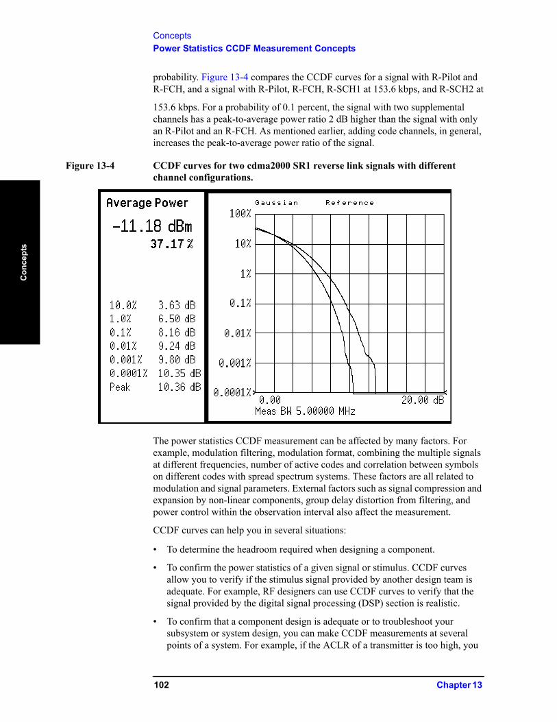
ConceptsPower Statistics CCDF Measurement Concepts
Con
cept
s
probability. Figure 13-4 compares the CCDF curves for a signal with R-Pilot and R-FCH, and a signal with R-Pilot, R-FCH, R-SCH1 at 153.6 kbps, and R-SCH2 at
153.6 kbps. For a probability of 0.1 percent, the signal with two supplemental channels has a peak-to-average power ratio 2 dB higher than the signal with only an R-Pilot and an R-FCH. As mentioned earlier, adding code channels, in general, increases the peak-to-average power ratio of the signal.
Figure 13-4 CCDF curves for two cdma2000 SR1 reverse link signals with different channel configurations.
The power statistics CCDF measurement can be affected by many factors. For example, modulation filtering, modulation format, combining the multiple signals at different frequencies, number of active codes and correlation between symbols on different codes with spread spectrum systems. These factors are all related to modulation and signal parameters. External factors such as signal compression and expansion by non-linear components, group delay distortion from filtering, and power control within the observation interval also affect the measurement.
CCDF curves can help you in several situations:
• To determine the headroom required when designing a component.
• To confirm the power statistics of a given signal or stimulus. CCDF curves allow you to verify if the stimulus signal provided by another design team is adequate. For example, RF designers can use CCDF curves to verify that the signal provided by the digital signal processing (DSP) section is realistic.
• To confirm that a component design is adequate or to troubleshoot your subsystem or system design, you can make CCDF measurements at several points of a system. For example, if the ACLR of a transmitter is too high, you
102 Chapter 13

ConceptsPower Statistics CCDF Measurement Concepts
Concepts
can make CCDF measurements at the input and output of the PA. If the PA design is correct, the curves will coincide. If the PA compresses the signal, the PAR of the signal is lower at the output of the PA (Figure 13-4 on page 102).
Measurement Method
The power measured in power statistics CCDF curves is actually instantaneous envelope power defined by the equation:
(where I and Q are the quadrature voltage components of the waveform and Zo is the characteristic impedance).
A CCDF curve is defined by how much time the waveform spends at or above a given power level. The percent of time the signal spends at or above the level defines the probability for that particular power level. To make the power statistics CCDF measurement, the instrument uses digital signal processing (DSP) to sample the input signal in the channel bandwidth.
The Gaussian distribution line as the band-limited gaussian noise CCDF reference line, the user-definable reference trace, and the currently measured trace can be displayed on a semi-log graph. If the currently measured trace is above the user reference trace, it means that the higher peak power levels against the average power are included in the input signal.
P I2 Q2+( ) Z0⁄=
Chapter 13 103
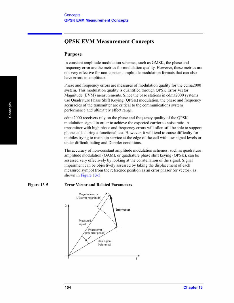
ConceptsQPSK EVM Measurement Concepts
Con
cept
s
QPSK EVM Measurement Concepts
Purpose
In constant amplitude modulation schemes, such as GMSK, the phase and frequency error are the metrics for modulation quality. However, these metrics are not very effective for non-constant amplitude modulation formats that can also have errors in amplitude.
Phase and frequency errors are measures of modulation quality for the cdma2000 system. This modulation quality is quantified through QPSK Error Vector Magnitude (EVM) measurements. Since the base stations in cdma2000 systems use Quadrature Phase Shift Keying (QPSK) modulation, the phase and frequency accuracies of the transmitter are critical to the communications system performance and ultimately affect range.
cdma2000 receivers rely on the phase and frequency quality of the QPSK modulation signal in order to achieve the expected carrier to noise ratio. A transmitter with high phase and frequency errors will often still be able to support phone calls during a functional test. However, it will tend to cause difficulty for mobiles trying to maintain service at the edge of the cell with low signal levels or under difficult fading and Doppler conditions.
The accuracy of non-constant amplitude modulation schemes, such as quadrature amplitude modulation (QAM), or quadrature phase shift keying (QPSK), can be assessed very effectively by looking at the constellation of the signal. Signal impairment can be objectively assessed by taking the displacement of each measured symbol from the reference position as an error phasor (or vector), as shown in Figure 13-5.
Figure 13-5 Error Vector and Related Parameters
Q
I
Magnitude error(I/Q error magnitude)
Measuredsignal
Ideal signal(reference)
Phase error(I/Q error phase)
Error vector
ø
104 Chapter 13
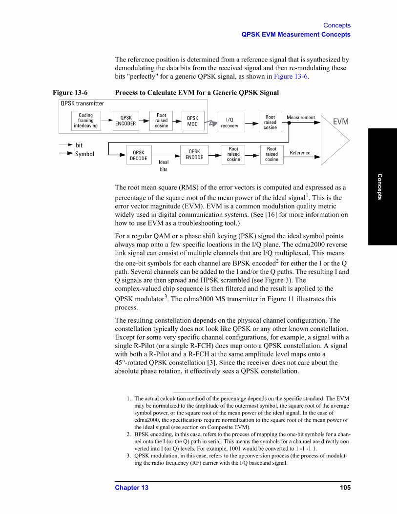
ConceptsQPSK EVM Measurement Concepts
Concepts
The reference position is determined from a reference signal that is synthesized by demodulating the data bits from the received signal and then re-modulating these bits "perfectly" for a generic QPSK signal, as shown in Figure 13-6.
Figure 13-6 Process to Calculate EVM for a Generic QPSK Signal
The root mean square (RMS) of the error vectors is computed and expressed as a percentage of the square root of the mean power of the ideal signal1. This is the error vector magnitude (EVM). EVM is a common modulation quality metric widely used in digital communication systems. (See [16] for more information on how to use EVM as a troubleshooting tool.)
For a regular QAM or a phase shift keying (PSK) signal the ideal symbol points always map onto a few specific locations in the I/Q plane. The cdma2000 reverse link signal can consist of multiple channels that are I/Q multiplexed. This means the one-bit symbols for each channel are BPSK encoded2 for either the I or the Q path. Several channels can be added to the I and/or the Q paths. The resulting I and Q signals are then spread and HPSK scrambled (see Figure 3). The complex-valued chip sequence is then filtered and the result is applied to the QPSK modulator3. The cdma2000 MS transmitter in Figure 11 illustrates this process.
The resulting constellation depends on the physical channel configuration. The constellation typically does not look like QPSK or any other known constellation. Except for some very specific channel configurations, for example, a signal with a single R-Pilot (or a single R-FCH) does map onto a QPSK constellation. A signal with both a R-Pilot and a R-FCH at the same amplitude level maps onto a 45°-rotated QPSK constellation [3]. Since the receiver does not care about the absolute phase rotation, it effectively sees a QPSK constellation.
QPSK transmitter
Codingframing
interleavingEVM
bitSymbol
Measurement
Reference
I/Qrecovery
QPSKMOD
Ideal
bits
Rootraisedcosine
Rootraisedcosine
QPSKENCODER
Rootraisedcosine
QPSKENCODE
Rootraisedcosine
QPSKDECODE
1. The actual calculation method of the percentage depends on the specific standard. The EVM may be normalized to the amplitude of the outermost symbol, the square root of the average symbol power, or the square root of the mean power of the ideal signal. In the case of cdma2000, the specifications require normalization to the square root of the mean power of the ideal signal (see section on Composite EVM).
2. BPSK encoding, in this case, refers to the process of mapping the one-bit symbols for a chan-nel onto the I (or the Q) path in serial. This means the symbols for a channel are directly con-verted into I (or Q) levels. For example, 1001 would be converted to 1 -1 -1 1.
3. QPSK modulation, in this case, refers to the upconversion process (the process of modulat-ing the radio frequency (RF) carrier with the I/Q baseband signal.
Chapter 13 105
ConceptsQPSK EVM Measurement Concepts
Con
cept
s
You can use a regular QPSK EVM measurement to evaluate the modulation quality of the transmitter for a single R-Pilot, a single R-FCH, or a signal with both at the same amplitude level. More complex signals cannot be analyzed with this measurement.
The signal analyzer may use either of the following methodologies to make a QPSK EVM measurement:
• Measure QPSK EVM on the received signal. Filter the recovered I/Q signal with the equalizer and complementary receiver filters and compare it with a reference signal calculated by filtering the demodulated signal with the transmitter, equalizer, and receiver filters See (a) in Figure 13-7 on page 107.
• Measure QPSK EVM on the transmitted signal. Compare the I/Q recovered signal directly with a reference signal calculated by filtering the ideal chips with the transmitter filter. See (b) in Figure 13-7 on page 107.
Both methods yield similar EVM results and you can use either of them to make valid modulation quality measurements of the MS transmitter; however, the resulting constellation looks different. The first method results in four discrete constellation points. The second method results in a fuzzy constellation, as shown in Figure 12a. The constellations for both methods are correct. The reason for the difference is that, for the first method, the constellation displays what the receiver sees after filtering, while the second method displays the constellation of the transmitted signal before applying any receiver filtering.
106 Chapter 13
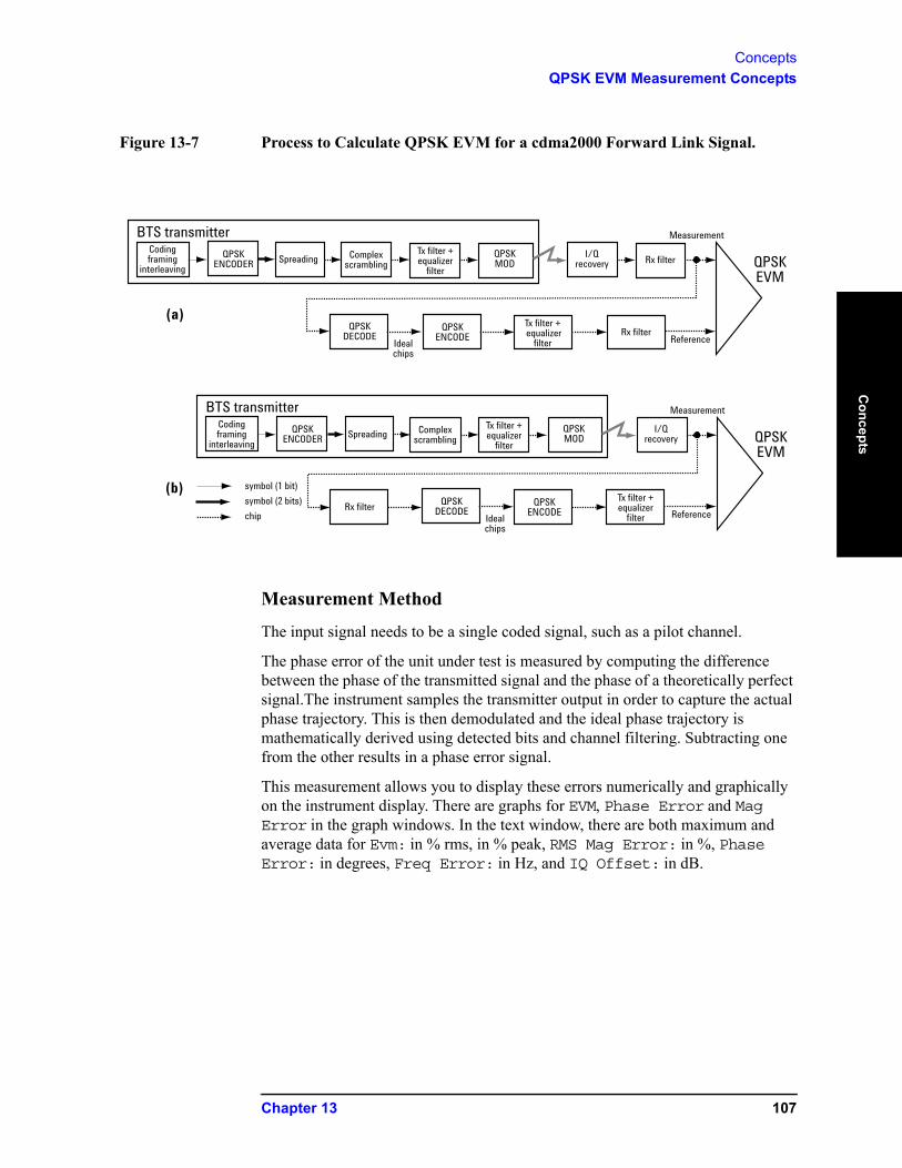
ConceptsQPSK EVM Measurement Concepts
Concepts
Figure 13-7 Process to Calculate QPSK EVM for a cdma2000 Forward Link Signal.
Measurement Method
The input signal needs to be a single coded signal, such as a pilot channel.
The phase error of the unit under test is measured by computing the difference between the phase of the transmitted signal and the phase of a theoretically perfect signal.The instrument samples the transmitter output in order to capture the actual phase trajectory. This is then demodulated and the ideal phase trajectory is mathematically derived using detected bits and channel filtering. Subtracting one from the other results in a phase error signal.
This measurement allows you to display these errors numerically and graphically on the instrument display. There are graphs for EVM, Phase Error and Mag Error in the graph windows. In the text window, there are both maximum and average data for Evm: in % rms, in % peak, RMS Mag Error: in %, Phase Error: in degrees, Freq Error: in Hz, and IQ Offset: in dB.
I/Qrecovery Rx filter
QPSKDECODE
QPSKENCODE
QPSKMOD
Measurement
Rx filterReferenceIdeal
chips
QPSKEVM
Codingframing
interleaving
BTS transmitterQPSK
ENCODER Spreading Complexscrambling
I/Qrecovery
QPSKDECODE
QPSKENCODE
QPSKMOD
Measurement
ReferenceIdealchips
QPSKEVM
symbol (1 bit)
symbol (2 bits)
chip
Codingframing
interleaving
BTS transmitterQPSK
ENCODER Spreading Complexscrambling
Rx filter
(a)
(b)
Tx filter + equalizer
filter
Tx filter + equalizer
filter
Tx filter + equalizer
filter
Tx filter + equalizer
filter
Chapter 13 107
ConceptsMonitor Spectrum Measurement Concepts
Con
cept
s
Monitor Spectrum Measurement Concepts
Purpose
The monitor spectrum measurement provides spectrum analysis capability for the instrument. It is used as a quick, convenient means of looking at the entire spectrum. While the look and feel are similar to the Spectrum Analyzer mode, the functionality is greatly reduced for easy operation. The main purpose of the measurement is to show the spectrum. The default span should cover an appropriate frequency range of the application.
Measurement Method
The measurement takes the sweep and acquires the data between the start frequency and stop frequency, then trace is displayed in the measurement window.
Troubleshooting Hints
Changes made by the user to advanced spectrum settings, particularly to ADC range settings, can inadvertently result in spectrum measurements that are invalid and cause error messages to appear. Care needs to be taken when using advanced features.
108 Chapter 13
ConceptsSpectrum Emission Mask Measurement Concepts
Concepts
Spectrum Emission Mask Measurement Concepts
Purpose
Spectrum Emission Mask measurements include the in-band and out-of-band spurious emissions. As it applies to cdma2000, it is the power contained in a specified frequency bandwidth at certain offsets relative to the total carrier power. It may also be expressed as a ratio of power spectral densities between the carrier and the specified offset frequency band.
As a composite measurement of out-of-channel emissions, the spectrum emission mask measurement combines both in-band and out-of-band specifications to provide useful figures-of-merit for spectral regrowth and emissions produced by components and circuit blocks without the rigor of performing a full spectrum emissions mask measurement.
Measurement Method
The spectrum emission mask measurement measures spurious signal levels in up to six pairs of offset/region frequencies and relates them to the carrier power. The reference channel integration bandwidth method is used to measure the carrier channel power and offset/region powers. When “Offset” is selected, spectrum emission mask measurements are made, relative to the carrier channel frequency bandwidth. When “Region” is selected, spurious emission absolute measurements are made, set by specifying start and stop RF frequencies. The upper frequency range limit is 3.678 GHz. The measurement screen is titled Spurious Emission.
The channel integration bandwidth is analyzed using the user defined resolution bandwidth (RBW), which is much narrower than the channel bandwidth. The measurement computes an average power of the channel or offset/region over a specified number of data acquisitions, automatically compensating for resolution bandwidth and noise bandwidth.
This measurement requires the user to specify measurement bandwidths of the carrier channel and each of the offset/region frequency pairs up to 5. Each pair may be defined with unique measurement bandwidths. The results are displayed both as relative power in dBc, and as absolute power in dBm.
Chapter 13 109

ConceptsSpurious Emissions Measurement Concepts
Con
cept
s
Spurious Emissions Measurement Concepts
Purpose
Spurious signals can be caused by different combinations of signals in the transmitter. The spurious emissions from the transmitter should be minimized to guarantee minimum interference with other frequency channels in the system. Harmonics are distortion products caused by nonlinear behavior in the transmitter. They are integer multiples of the transmitted signal carrier frequency.
This measurement verifies the frequency ranges of interest are free of interference by measuring the spurious signals specified by the user defined range table.
Measurement Method
The table-driven measurement has the flexibility to set up custom parameters such as frequency, span, resolution bandwidth, and video bandwidth.
For each range that you specify and activate, the analyzer scans the band using the specified Range Table settings. Then using the Peak Excursion and Peak Threshold values determines which spurs to report.
As each band is swept, any signal which is above the Peak Threshold value and has a peak excursion of greater than the Peak Excursion value will be added to a list of spurs displayed in the lower results window. A total of 200 spurs can be recorded for one measurement, with a limit of 10 spurs per frequency range. To improve repeatability, you can increase the number of averages.
From the spurs in the list, those with peak amplitude greater than the Absolute Limit for that range will be logged as a measurement failure and denoted by an 'F' in the 'Amplitude' column of the table. If no spurs are reported, but the measured trace exceeds the limit line for any range, the fail flag is set to fail.
This measurement has the ability to display two traces using different detectors on the display simultaneously. All spur detection and limit line testing are only applied to the trace associated with Detector 1, which will be colored yellow. The trace associated with Detector 2 will be colored cyan.
If the sweep time for the range exceeds 2 seconds, a flashing message “Sweeping...Please Wait” will appear in the annunciator area. This advises you that the time to complete the sweep is between 2 and 2000 seconds, and is used as without it the display would appear stagnant and you may think the measurement is not functional.
110 Chapter 13
ConceptsIQ Waveform Measurement Concepts
Concepts
IQ Waveform Measurement Concepts
Purpose
The waveform measurement is a generic measurement for viewing the input signal waveforms in the time domain. This measurement is how the instrument performs the zero span functionality found in traditional spectrum analyzers.
Basic mode waveform measurement data may be displayed using either a Signal Envelope window, or an I/Q window which shows the I and Q signal waveforms in parameters of voltage versus time. The advantage of having an I/Q view available while making a waveform measurement is that it allows you to view complex components of the same signal without changing settings or measurements.
The waveform measurement can be used to perform general purpose power measurements in the time domain with excellent accuracy.
Measurement Method
The instrument makes repeated power measurements at a set frequency, similar to the way a swept-tuned spectrum analyzer makes zero span measurements. The input analog signal is converted to a digital signal, which then is processed into a representation of a waveform measurement. The measurement relies on a high rate of sampling to create an accurate representation of a time domain signal.
Chapter 13 111
ConceptsOther Sources of Measurement Information
Con
cept
s
Other Sources of Measurement InformationAdditional measurement application information is available through your local Agilent Technologies sales and service office. The following application notes treat digital communications measurements in much greater detail than discussed in this measurement guide.
• Application Note 1298
Digital Modulation in Communications Systems - An IntroductionAgilent part number 5965-7160E
• Application Note 1311
Understanding CDMA Measurements for Base Stations and Their ComponentsAgilent part number 5968-0953E
• Application Note 1335
HPSK Spreading for 3GAgilent part number 5968-8438E
• Application Note 1357
Designing and Testing cdma2000 Base StationsAgilent part number 5980-1303E
• Application Note 1358
Designing and Testing cdma2000 Mobile StationsAgilent part number 5980-1237E
• Application Note
Characterizing Digitally Modulated Signals with CCDF CurvesAgilent part number 5968-5858E
Instrument Updates at www.agilent.com
These web locations can be used to access the latest information about the instrument, including the latest firmware version.
http://www.agilent.com/find/mxa
112 Chapter 13
ConceptsReferences
Concepts
References[1] Understanding CDMA Measurements for Base Stations and Their Components, Application Note 1311, literature number 5968-0953E.
[2] Ken Thompson, “Concepts of cdma2000,” Wireless Symposium, 999.
[3] HPSK Spreading for 3G, Application Note 1335, literature number 5968-8438E.
[4] Designing and Testing W-CDMA Base Stations, Application Note 1355, literature number 5980-1239E.
Chapter 13 113
ConceptsReferences
Con
cept
s
114 Chapter 13
14 Programming Examples
• The programming examples were written for use on an IBM compatible PC.
• The programming examples use C, Visual Basic, or VEE programming languages.
• The programming examples use VISA interfaces (GPIB, LAN, or USB).
• Some of the examples use the IVI-COM drivers.
Interchangeable Virtual Instruments COM (IVI-COM) drivers: Develop system automation software easily and quickly. IVI-COM drivers take full advantage of application development environments such as Visual Studio using Visual Basic, C# or Visual C++ as well as Agilent's Test and Measurement Toolkit. You can now develop application programs that are portable across computer platforms and I/O interfaces. With IVI-COM drivers you do not need to have in depth test instrument knowledge to develop sophisticated measurement software. IVI-COM drivers provide a compatible interface to all. COM environments. The IVI-COM software drivers can be found at the URL:http://www.agilent.com/find/ivi-com
• Most of the examples are written in C, Visual Basic, VEE, or LabVIew using the Agilent VISA transition library.
The Agilent I/O Libraries Suite must be installed and the GPIB card, USB to GPIB interface, or Lan interface USB interface configured. The latest Agilent I/O Libraries Suite is available: www.agilent.com/find/iolib
• The STATus subsystem of commands is used to monitor and query hardware status. These hardware registers monitor various events and conditions in the instrument. Details about the use of these commands and registers can be found in the manual/help in the Utility Functions section on the STATus subsystem.
Visual Basic is a registered trademark of Microsoft Corporation.
85

Programming ExamplesAvailable Programing Examples
Prog
ram
min
g Ex
ampl
es
Available Programing ExamplesThe following examples work with a Spectrum Analyzer. These examples use one of the following programming languages: Visual Basic® 6, Visual Basic.NET®, MS Excel®, C++, ANSI C, C#.NET, and Agilent VEE Pro.
These examples are available in either the “progexamples” directory on the Agilent Technologies Spectrum Analyzer documentation CD-ROM or the “progexamples” directory in the analyzer. The file names for each example is listed at the end of the example description. The examples can also be found on the Agilent Technologies, Inc. web site at URL:
http://www.agilent.com/find/sa_programming
NOTE These examples have all been test and validated as functional in the Spectrum Analyzer mode. They have not been tested in all other modes. However, they should work in all other modes except where exceptions are noted.
Programming using Visual Basic® 6, Visual Basic.NET® and MS Excel®:
• Transfer Screen Images from your Spectrum Analyzer using Visual Basic 6
This example program stores the current screen image on the instrument flash memory as “D:\PICTURE.PNG”. It then transfers the image over GPIB or LAN and stores the image on your PC in the current directory as “PICTURE.PNG”. The file “D:\PICTURE.PNG” is then deleted on the instrument flash memory.
File name: _screen.bas
• Binary Block Trace data transfer from your Spectrum Analyzer using Visual Basic 6
This example program queries the IDN string from the instrument and then reads the trace data in Spectrum Analysis mode in binary format (Real,32 or Real,64 or Int,32). The data is then stored to a file “bintrace.txt”. This data transfer method is faster than the default ASCII transfer mode, because less data is sent over the bus.
File name: bintrace.bas
Programming using C++, ANSI C and C#.NET:
• Serial Poll for Sweep Complete using C++
This example demonstrates how to:
1. Perform an instrument sweep. 2. Poll the instrument to determine when the operation is complete.3. Perform an instrument sweep.
File name: _Sweep.c
86 Chapter 14
Programming ExamplesAvailable Programing Examples
Programm
ing Examples
• Service Request Method (SRQ) determines when a measurement is done by waiting for SRQ and reading Status Register using C++.
This example demonstrates how:
1. Set the service request mask to assert SRQ when either a measurement is uncalibrated or an error message has occurred,
2. Initiate a sweep and wait for the SRQ interrupt,3. Poll all instruments and report the nature of the * interrupt on the spectrum
analyzer.
The STATus subsystem of commands is used to monitor and query hardware status. These hardware registers monitor various events and conditions in the instrument. Details about the use of these commands and registers can be found in the manual/help in the Utility Functions section on the STATus subsystem.
File name: _SRQ.C
• Relative Band Power Markers using C++
This example demonstrates how to set markers as Band Power Markers and obtain their band power relative to another specified marker.
File name: _BPM.c
• Trace Detector/Couple Markers using C++
This example demonstrates how to:
1. Set different types of traces (max hold, clear and write, min hold) 2. Set markers to specified traces 3. Couple markers
Note: The Spectrum Analyzer is capable of multiple simultaneous detectors (i.e. peak detector for max hold, sample for clear and write, and negative peak for min hold).
File name: _tracecouple.c
• Phase Noise using C++
This example demonstrates how to:
1. Remove instrument noise from the phase noise2. Calculate the power difference between 2 traces
File name: _phasenoise.c
Programming using Agilent VEE Pro:
• Transfer Screen Images from my Spectrum Analyzer using Agilent VEE Pro
This example program stores the current screen image on the instrument flash memory as “D:\scr.png”. It then transfers the image over GPIB and stores the image on your PC in the desired directory as “capture.gif”. The file “D:\scr.png” is then deleted on the instrument flash memory.
File name: _ScreenCapture.vee
Chapter 14 87
Programming ExamplesAvailable Programing Examples
Prog
ram
min
g Ex
ampl
es
• Transfer Trace Data data transfer using Agilent VEE Pro
This example program transfers the trace data from your Spectrum Analyzer. The program queries the IDN string from the instrument and supports Integer 32, real 32, real 64 and ASCII data. The program returns 1001 trace points for the signal analyzer.
File name: transfertrace.vee
88 Chapter 14
Programming ExamplesProgramming Fundamentals
Programm
ing Examples
Programming Fundamentals• “SCPI Language Basics” on page 90
• “Improving Measurement Speed” on page 97
• “Programming in C Using the VTL” on page 101
Chapter 14 89
Programming ExamplesProgramming Fundamentals
Prog
ram
min
g Ex
ampl
es
SCPI Language Basics
This section is not intended to teach you everything about the SCPI (Standard Commands for Programmable Instruments) programming language. The SCPI Consortium or IEEE can provide that level of detailed information. For more information refer to the websites for the IEEE Standard 488.1 (IEEE Standard Digital Interface for Programmable Instrumentation).
Topics covered in this chapter include:
• “Command Keywords and Syntax” on page 90
• “Creating Valid Commands” on page 90
• “Special Characters in Commands” on page 91
• “Parameters in Commands” on page 92
• “Putting Multiple Commands on the Same Line” on page 94
Command Keywords and Syntax
A typical command is made up of keywords set off by colons. The keywords are followed by parameters that can be followed by optional units.
Example: SENSe:FREQuency:STARt 1.5 MHZ
The instrument does not distinguish between upper and lower case letters. In the documentation, upper case letters indicate the short form of the keyword. The lower case letters, indicate the long form of the keyword. Either form may be used in the command.
Example: Sens:Freq:Star 1.5 mhz
is the same as SENSE:FREQ:start 1.5 MHz
NOTE The command SENS:FREQU:STAR would not be valid because FREQU is neither the short, nor the long form of the command. Only the short and long forms of the keywords are allowed in valid commands.
Creating Valid Commands
Commands are not case sensitive and there are often many different ways of writing a particular command. These are examples of valid commands for a given
90 Chapter 14
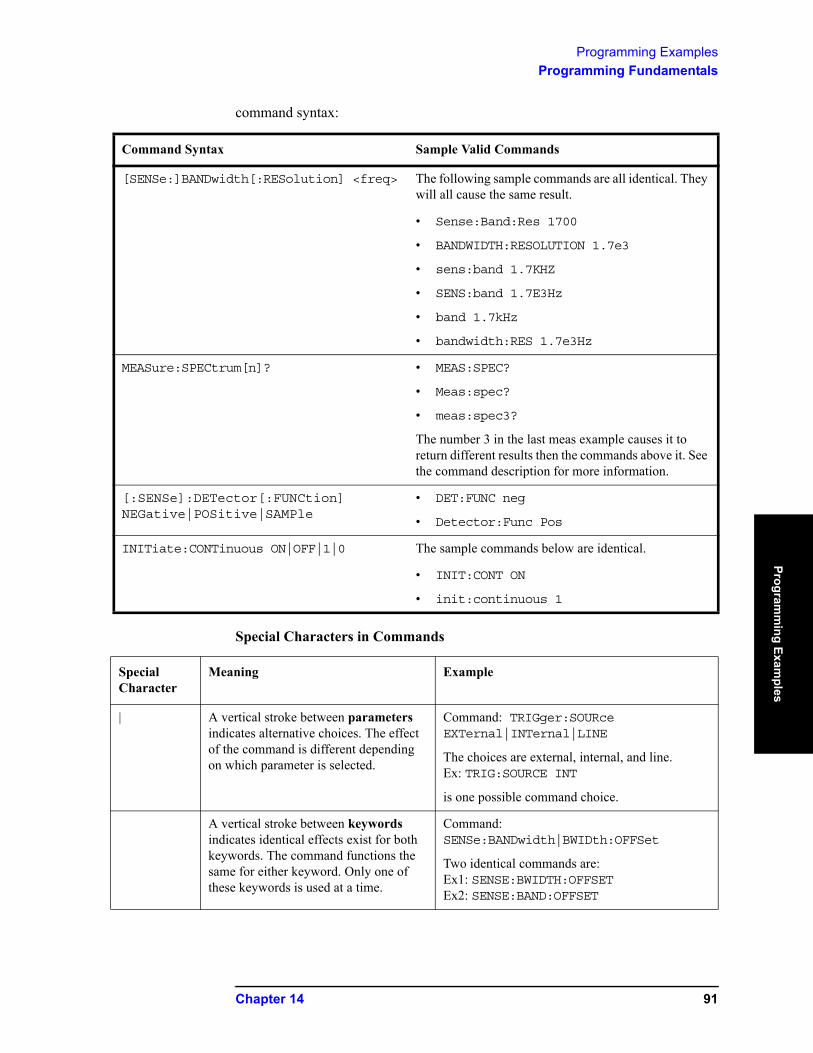
Programming ExamplesProgramming Fundamentals
Programm
ing Examples
command syntax:
Special Characters in Commands
Command Syntax Sample Valid Commands
[SENSe:]BANDwidth[:RESolution] <freq> The following sample commands are all identical. They will all cause the same result.
• Sense:Band:Res 1700
• BANDWIDTH:RESOLUTION 1.7e3
• sens:band 1.7KHZ
• SENS:band 1.7E3Hz
• band 1.7kHz
• bandwidth:RES 1.7e3Hz
MEASure:SPECtrum[n]? • MEAS:SPEC?
• Meas:spec?
• meas:spec3?
The number 3 in the last meas example causes it to return different results then the commands above it. See the command description for more information.
[:SENSe]:DETector[:FUNCtion] NEGative|POSitive|SAMPle
• DET:FUNC neg
• Detector:Func Pos
INITiate:CONTinuous ON|OFF|1|0 The sample commands below are identical.
• INIT:CONT ON
• init:continuous 1
Special Character
Meaning Example
| A vertical stroke between parameters indicates alternative choices. The effect of the command is different depending on which parameter is selected.
Command: TRIGger:SOURce EXTernal|INTernal|LINE
The choices are external, internal, and line.Ex: TRIG:SOURCE INT
is one possible command choice.
A vertical stroke between keywords indicates identical effects exist for both keywords. The command functions the same for either keyword. Only one of these keywords is used at a time.
Command: SENSe:BANDwidth|BWIDth:OFFSet
Two identical commands are:Ex1: SENSE:BWIDTH:OFFSET Ex2: SENSE:BAND:OFFSET
Chapter 14 91
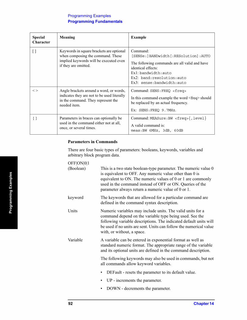
Programming ExamplesProgramming Fundamentals
Prog
ram
min
g Ex
ampl
es
Parameters in Commands
There are four basic types of parameters: booleans, keywords, variables and arbitrary block program data.
OFF|ON|0|1(Boolean) This is a two state boolean-type parameter. The numeric value 0
is equivalent to OFF. Any numeric value other than 0 is equivalent to ON. The numeric values of 0 or 1 are commonly used in the command instead of OFF or ON. Queries of the parameter always return a numeric value of 0 or 1.
keyword The keywords that are allowed for a particular command are defined in the command syntax description.
Units Numeric variables may include units. The valid units for a command depend on the variable type being used. See the following variable descriptions. The indicated default units will be used if no units are sent. Units can follow the numerical value with, or without, a space.
Variable A variable can be entered in exponential format as well as standard numeric format. The appropriate range of the variable and its optional units are defined in the command description.
The following keywords may also be used in commands, but not all commands allow keyword variables.
• DEFault - resets the parameter to its default value.
• UP - increments the parameter.
• DOWN - decrements the parameter.
[ ] Keywords in square brackets are optional when composing the command. These implied keywords will be executed even if they are omitted.
Command: [SENSe:]BANDwidth[:RESolution]:AUTO
The following commands are all valid and have identical effects:Ex1: bandwidth:autoEx2: band:resolution:autoEx3: sense:bandwidth:auto
< > Angle brackets around a word, or words, indicates they are not to be used literally in the command. They represent the needed item.
Command: SENS:FREQ <freq>
In this command example the word <freq> should be replaced by an actual frequency.
Ex: SENS:FREQ 9.7MHz.
{ } Parameters in braces can optionally be used in the command either not at all, once, or several times.
Command: MEASure:BW <freq>{,level}
A valid command is:meas:BW 6MHz, 3dB, 60dB
Special Character
Meaning Example
92 Chapter 14

Programming ExamplesProgramming Fundamentals
Programm
ing Examples
• MINimum - sets the parameter to the smallest possible value.
• MAXimum - sets the parameter to the largest possible value.
The numeric value for the function MINimum, MAXimum, or DEFault can be queried by adding the keyword to the command in its query form. The keyword must be entered following the question mark.
Example query: SENSE:FREQ:CENTER? MAX
Variable Parameters
<integer> is an integer value with no units.
<real> Is a floating point number with no units.
<freq><bandwidth> Is a positive rational number followed by optional units. The
default unit is Hertz. Acceptable units include: Hz, kHz, MHz, GHz.
<time><seconds> Is a rational number followed by optional units. The default
units are seconds. Acceptable units include: ks, s, ms, µs, ns.
<voltage> Is a rational number followed by optional units. The default units are Volts. Acceptable units include: V, mV, µV, nV
<current> Is a rational number followed by optional units. The default units are Amperes. Acceptable units include: A, mA, µA, nA.
<power> Is a rational number followed by optional units. The default units are W. Acceptable units include: mAW, kW, W, mW, µW, nW, pW.
<ampl> Is a rational number followed by optional units. The default units are dBm. Acceptable units include: dBm, dBmV, dBµV.
<rel_power><rel_ampl> Is a positive rational number followed by optional units. The
default units are dB. Acceptable units include: dB.
<percent> Is a rational number between 0 and 100. You can either use no units or use PCT.
<angle><degrees> Is a rational number followed by optional units. The default
units are degrees. Acceptable units include: DEG, RAD.
<string> Is a series of alpha numeric characters.
<bit_pattern> Specifies a series of bits rather than a numeric value. The bit series is the binary representation of a numeric value. There are no units.
Chapter 14 93
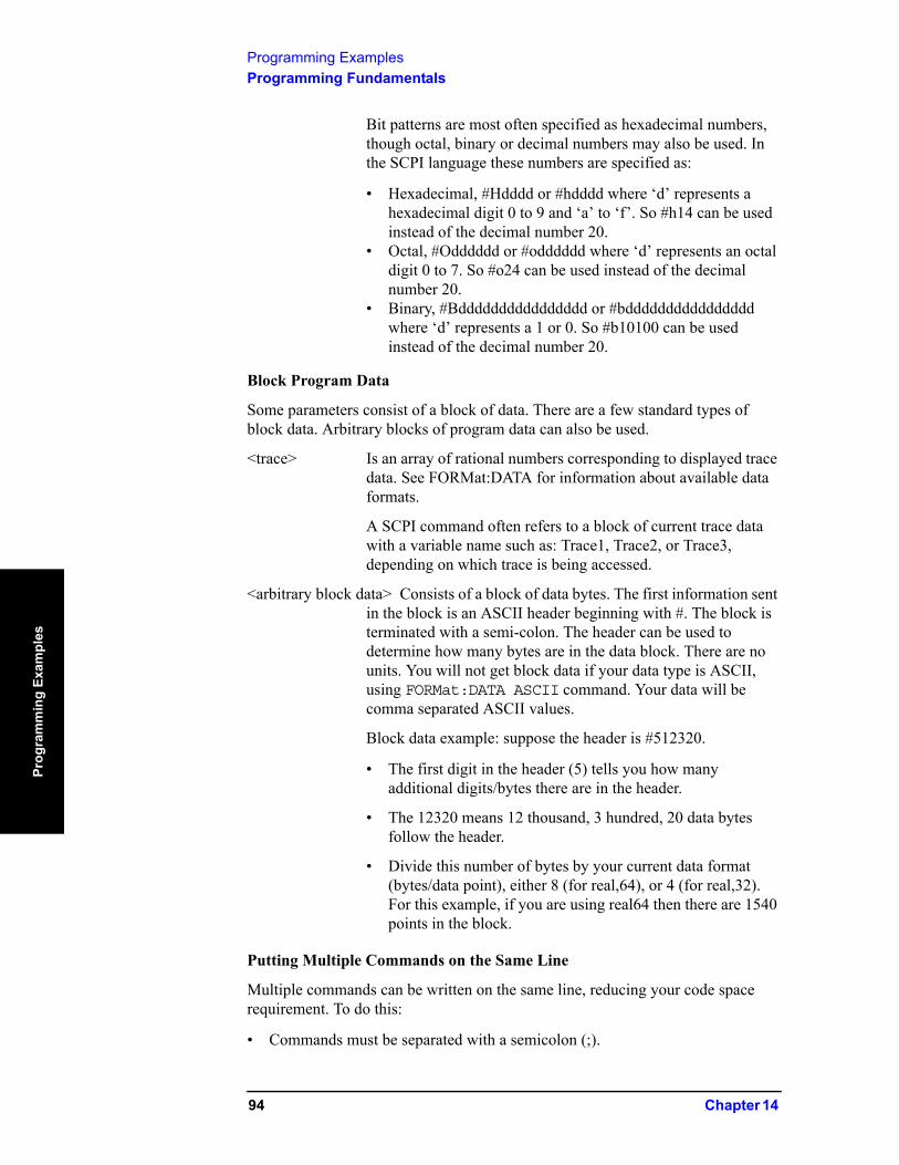
Programming ExamplesProgramming Fundamentals
Prog
ram
min
g Ex
ampl
es
Bit patterns are most often specified as hexadecimal numbers, though octal, binary or decimal numbers may also be used. In the SCPI language these numbers are specified as:
• Hexadecimal, #Hdddd or #hdddd where ‘d’ represents a hexadecimal digit 0 to 9 and ‘a’ to ‘f’. So #h14 can be used instead of the decimal number 20.
• Octal, #Odddddd or #odddddd where ‘d’ represents an octal digit 0 to 7. So #o24 can be used instead of the decimal number 20.
• Binary, #Bdddddddddddddddd or #bdddddddddddddddd where ‘d’ represents a 1 or 0. So #b10100 can be used instead of the decimal number 20.
Block Program Data
Some parameters consist of a block of data. There are a few standard types of block data. Arbitrary blocks of program data can also be used.
<trace> Is an array of rational numbers corresponding to displayed trace data. See FORMat:DATA for information about available data formats.
A SCPI command often refers to a block of current trace data with a variable name such as: Trace1, Trace2, or Trace3, depending on which trace is being accessed.
<arbitrary block data> Consists of a block of data bytes. The first information sent in the block is an ASCII header beginning with #. The block is terminated with a semi-colon. The header can be used to determine how many bytes are in the data block. There are no units. You will not get block data if your data type is ASCII, using FORMat:DATA ASCII command. Your data will be comma separated ASCII values.
Block data example: suppose the header is #512320.
• The first digit in the header (5) tells you how many additional digits/bytes there are in the header.
• The 12320 means 12 thousand, 3 hundred, 20 data bytes follow the header.
• Divide this number of bytes by your current data format (bytes/data point), either 8 (for real,64), or 4 (for real,32). For this example, if you are using real64 then there are 1540 points in the block.
Putting Multiple Commands on the Same Line
Multiple commands can be written on the same line, reducing your code space requirement. To do this:
• Commands must be separated with a semicolon (;).
94 Chapter 14
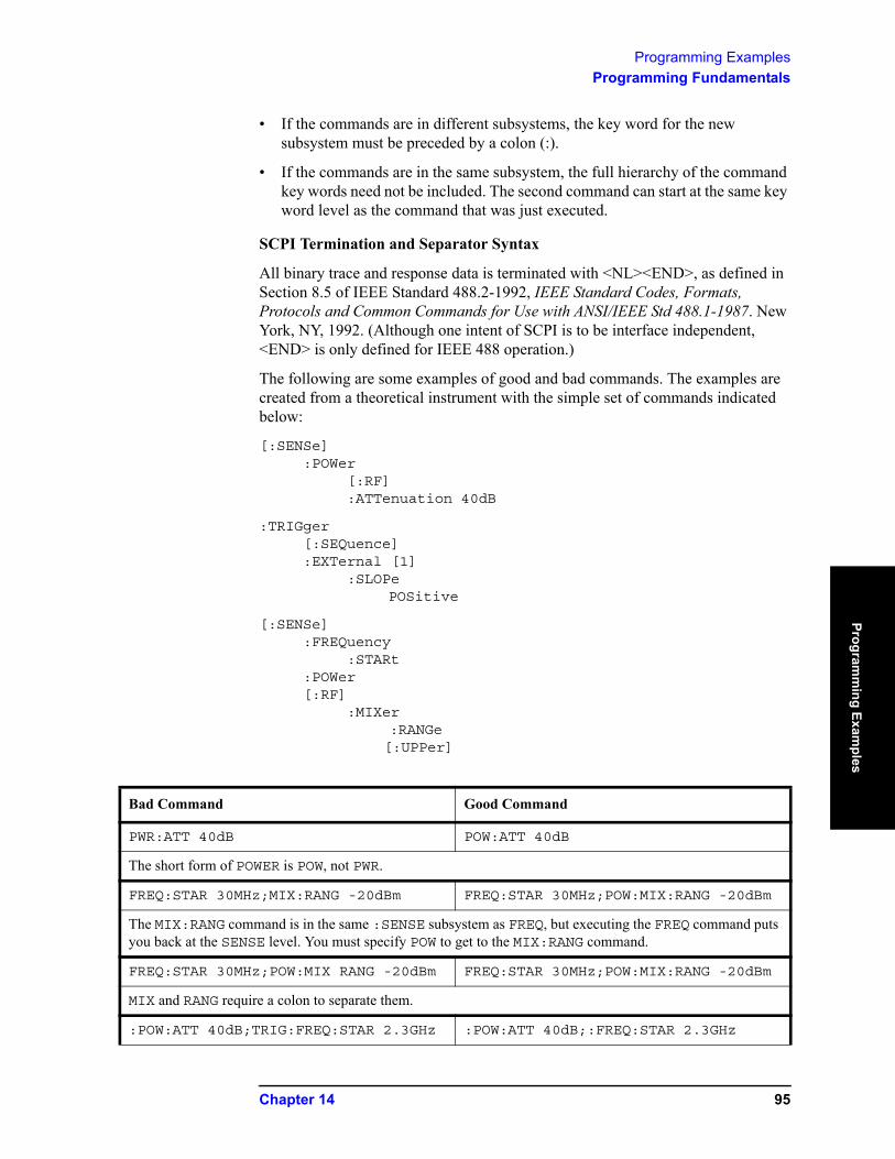
Programming ExamplesProgramming Fundamentals
Programm
ing Examples
• If the commands are in different subsystems, the key word for the new subsystem must be preceded by a colon (:).
• If the commands are in the same subsystem, the full hierarchy of the command key words need not be included. The second command can start at the same key word level as the command that was just executed.
SCPI Termination and Separator Syntax
All binary trace and response data is terminated with <NL><END>, as defined in Section 8.5 of IEEE Standard 488.2-1992, IEEE Standard Codes, Formats, Protocols and Common Commands for Use with ANSI/IEEE Std 488.1-1987. New York, NY, 1992. (Although one intent of SCPI is to be interface independent, <END> is only defined for IEEE 488 operation.)
The following are some examples of good and bad commands. The examples are created from a theoretical instrument with the simple set of commands indicated below:
[:SENSe]:POWer
[:RF]:ATTenuation 40dB
:TRIGger [:SEQuence]:EXTernal [1]
:SLOPePOSitive
[:SENSe]:FREQuency
:STARt:POWer[:RF]
:MIXer:RANGe[:UPPer]
Bad Command Good Command
PWR:ATT 40dB POW:ATT 40dB
The short form of POWER is POW, not PWR.
FREQ:STAR 30MHz;MIX:RANG -20dBm FREQ:STAR 30MHz;POW:MIX:RANG -20dBm
The MIX:RANG command is in the same :SENSE subsystem as FREQ, but executing the FREQ command puts you back at the SENSE level. You must specify POW to get to the MIX:RANG command.
FREQ:STAR 30MHz;POW:MIX RANG -20dBm FREQ:STAR 30MHz;POW:MIX:RANG -20dBm
MIX and RANG require a colon to separate them.
:POW:ATT 40dB;TRIG:FREQ:STAR 2.3GHz :POW:ATT 40dB;:FREQ:STAR 2.3GHz
Chapter 14 95
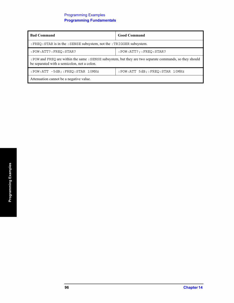
Programming ExamplesProgramming Fundamentals
Prog
ram
min
g Ex
ampl
es
:FREQ:STAR is in the :SENSE subsystem, not the :TRIGGER subsystem.
:POW:ATT?:FREQ:STAR? :POW:ATT?;:FREQ:STAR?
:POW and FREQ are within the same :SENSE subsystem, but they are two separate commands, so they should be separated with a semicolon, not a colon.
:POW:ATT -5dB;:FREQ:STAR 10MHz :POW:ATT 5dB;:FREQ:STAR 10MHz
Attenuation cannot be a negative value.
Bad Command Good Command
96 Chapter 14
Programming ExamplesProgramming Fundamentals
Programm
ing Examples
Improving Measurement Speed
There are a number of things you can do in your programs to make them run faster:
“Turn off the display updates” on page 97
“Use binary data format instead of ASCII” on page 97
“Minimize the number of GPIB transactions” on page 98
“Consider using USB or LAN instead of GPIB” on page 98
“Minimize DUT/instrument setup changes” on page 98
“Avoid automatic attenuator setting” on page 99
“Avoid using RFBurst trigger for single burst signals” on page 99
Turn off the display updates
:DISPlay:ENABle OFF turns off the display. That is, the data may still be visible, but it will no longer be updated. Updating the display slows down the measurement. For remote testing, since the computer is processing the data rather than a person, there is no need to display the data on the analyzer screen.
Use binary data format instead of ASCII
The ASCII data format is the instrument default since it is easier for people to understand and is required by SCPI for *RST. However, data input/output is faster using the binary formats.
:FORMat:DATA REAL,64 selects the 64-bit binary data format for all your numerical data queries. You may need to swap the byte order if you are using a PC rather than UNIX. NORMal is the default byte order. Use :FORMat:BORDer SWAP to change the byte order so that the least significant byte is sent first. (Real,32 which is smaller and somewhat faster, should only be used if you do not need full resolution for your data. Some frequency data may require full 64-bit resolution.)
When using the binary format, data is sent in a block of bytes with an ASCII header. A data query would return the block of data in the following format: #DNNN<nnn binary data bytes>
To parse the data:
• Read two characters (#D), where D tells you how many N characters follow the D character.
• Read D characters, the resulting integer specifies the number of data bytes sent.• Read the bytes into a real array.
For example, suppose the header is #512320.
• The first character/digit in the header (5) tells you how many additional digits there are in the header.
• The 12320 means 12 thousand, 3 hundred, 20 data bytes follow the header.• Divide this number of bytes by your current data format (bytes/data point), 8
Chapter 14 97
Programming ExamplesProgramming Fundamentals
Prog
ram
min
g Ex
ampl
es
for real,64. For this example, there are 1540 data points in the block of data.
Minimize the number of GPIB transactions
When you are using the GPIB for control of your instrument, each transaction requires driver overhead and bus handshaking, so minimizing these transactions reduces the time used.
• You can reduce bus transactions by sending multiple commands per transaction. See the information on “Putting Multiple Commands on the Same Line” in the SCPI Language Basics section.
• If you are making the same measurement multiple times with small changes in the measurement setup, use the READ command. It is faster then using INITiate and FETCh.
Consider using USB or LAN instead of GPIB
USB and LAN allow faster data input and output. This is especially important if you are moving large blocks of data. You will not get this improved throughput using LAN if there is excessive LAN traffic (that is, your test instrument is connected to a very busy enterprise LAN). You may want to use a private LAN that is only for your test system.
Minimize DUT/instrument setup changes
• Some instrument setup parameters are common to multiple measurements. You should look at your measurement process with an eye toward minimizing setup changes. If your test process involves nested loops, make sure that the inner-most loop is the fastest. Also, check if the loops could be nested in a different order to reduce the number of parameter changes as you step through the test.
• Are you are using the measurements under the Meas key? Remember that if you have already set your Meas Setup parameters for a measurement, and you want to make another one of these measurements later, use READ:<meas>?. The MEASure:<meas>?. command resets all the settings to the defaults, while READ changes back to that measurement without changing the setup parameters from the previous use.
• Are you are using the Measurements under the Meas key? Remember that Mode Setup parameters remain constant across all the measurements in that mode (for example, center/channel frequency, amplitude, radio standard, input selection, trigger setup). You do not have to re-initialize them each time you change to a different measurement.
Avoid unnecessary use of *RST
Remember that while *RST does not change the current Mode, it presets all the measurements and settings to their factory defaults. This forces you to reset your analyzer measurement settings even if they use similar mode setup or measurement settings. See Minimize DUT/instrument setup changes. (Also note that *RST may put the instrument in single measurement/sweep for some modes.)
98 Chapter 14
Programming ExamplesProgramming Fundamentals
Programm
ing Examples
Avoid automatic attenuator setting
Many of the one-button measurements use an internal process for automatically setting the value of the attenuator. It requires measuring an initial burst to identify the proper attenuator setting before the next burst can be measured properly. If you know the amount of attenuation or the signal level needed for your measurement, just set it.
Note that spurious types of measurements must be done with the attenuator set to automatic (for measurements like: output RF spectrum, transmit spurs, adjacent channel power, spectrum emission mask). These types of measurements start by tuning to the signal, then they tune away from it and must be able to reset the attenuation value as needed.
Avoid using RFBurst trigger for single burst signals
RFBurst triggering works best when measuring signals with repetitive bursts. For a non-repetitive or single burst signals, use the IF (video) trigger or external trigger, depending on what you have available.
RFBurst triggering depends on its establishment of a valid triggering reference level, based on previous bursts. If you only have a single burst, the peak detection nature of this triggering function, may result in the trigger being done at the wrong level/point generating incorrect data, or it may not trigger at all.
Are you making a single burst measurement? To get consistent triggering and good data for this type of measurement application, you need to synchronize the triggering of the DUT with the analyzer. You should use the analyzer internal status system for this.
The first step in this process is to initialize the status register mask to look for the “waiting for trigger” condition (bit 5). Use :STATus:OPERation:ENABle 32
Then, in the measurement loop:
1. :STATus:OPERation:EVENt? This query of the operation event register is to clear the current register contents.
2. :READ:PVT? initiates a measurement (in this example, for GSM power versus time) using the previous setup. The measurement will then be waiting for the trigger.
Make sure the attenuation is set manually. Do NOT use automatic attenuation as this requires an additional burst to determine the proper attenuation level before the measurement can be made.
3. Create a small loop that will serial poll the instrument for a status byte value of binary 128. Then wait 1 msec (100 ms if the display is left on/enabled) before checking again, to keep the bus traffic down. These two commands are repeated until the condition is set, so we know that the trigger is armed and ready.
4. Trigger your DUT to send the burst.
5. Return the measurement data to your computer.
Chapter 14 99

Programming ExamplesProgramming Fundamentals
Prog
ram
min
g Ex
ampl
es
NOTE This process cannot be done with the current VXI plug-n-play driver implementation. You will need to use the previous SCPI commands.
100 Chapter 14
Programming ExamplesProgramming Fundamentals
Programm
ing Examples
Programming in C Using the VTL
The programming examples that are provided are written using the C programming language and the Agilent VTL (VISA transition library). This section includes some basic information about programming in the C language. Note that some of this information may not be relevant to your particular application. (For example, if you are not using VXI instruments, the VXI references will not be relevant).
Refer to your C programming language documentation for more details. (This information is taken from the manual “VISA Transition Library”, part number E2090-90026.) The following topics are included:
“Typical Example Program Contents” on page 101“Linking to VTL Libraries” on page 102“Compiling and Linking a VTL Program” on page 102“Example Program” on page 103“Including the VISA Declarations File” on page 104“Opening a Session” on page 104“Device Sessions” on page 105“Addressing a Session” on page 106“Closing a Session” on page 107
Typical Example Program Contents
The following is a summary of the VTL function calls used in the example programs.
visa.h This file is included at the beginning of the file to provide the function prototypes and constants defined by VTL.
ViSession The ViSession is a VTL data type. Each object that will establish a communication channel must be defined as ViSession.
viOpenDefaultRM You must first open a session with the default resource manager with the viOpenDefaultRM function. This function will initialize the default resource manager and return a pointer to that resource manager session.
viOpen This function establishes a communication channel with the device specified. A session identifier that can be used with other VTL functions is returned. This call must be made for each device you will be using.
viPrintfviScanf These are the VTL formatted I/O functions that are patterned
after those used in the C programming language. The viPrintf call sends the IEEE 488.2 *RST command to the instrument and puts it in a known state. The viPrintf call is used again to query for the device identification (*IDN?). The viScanf call is then used to read the results.
Chapter 14 101
Programming ExamplesProgramming Fundamentals
Prog
ram
min
g Ex
ampl
es
viClose This function must be used to close each session. When you close a device session, all data structures that had been allocated for the session will be de-allocated. When you close the default manager session, all sessions opened using the default manager session will be closed.
Linking to VTL Libraries
Your application must link to one of the VTL import libraries:
32-bit Version:
C:\VXIPNP\WIN95\LIB\MSC\VISA32.LIB for Microsoft compilers
C:\VXIPNP\WIN95\LIB\BC\VISA32.LIB for Borland compilers
16-bit Version:
C:\VXIPNP\WIN\LIB\MSC\VISA.LIB for Microsoft compilers
C:\VXIPNP\WIN\LIB\BC\VISA.LIB for Borland compilers
See the following section, “Compiling and Linking a VTL Program” for information on how to use the VTL run-time libraries.
Compiling and Linking a VTL Program
32-bit Applications
The following is a summary of important compiler-specific considerations for several C/C++ compiler products when developing WIN32 applications.
For Microsoft Visual C++ version 2.0 compilers:
• Select Project | Update All Dependencies from the menu.
• Select Project | Settings from the menu. Click on the C/C++ button. Select Code Generation from the Use Run-Time Libraries list box. VTL requires these definitions for WIN32. Click OK to close the dialog boxes.
• Select Project | Settings from the menu. Click on the Link button and add visa32.lib to the Object / Library Modules list box. Optionally, you may add the library directly to your project file. Click OK to close the dialog boxes.
• You may wish to add the include file and library file search paths. They are set by doing the following:
1. Select Tools | Options from the menu.
2. Click Directories to set the include file path.
3. Select Include Files from the Show Directories For list box.
4. Click Add and type in the following: C:\VXIPNP\WIN95\INCLUDE
5. Select Library Files from the Show Directories For list box.
102 Chapter 14
Programming ExamplesProgramming Fundamentals
Programm
ing Examples
6. Click Add and type in the following: C:\VXIPNP\WIN95\LIB\MSC
For Borland C++ version 4.0 compilers:
• You may wish to add the include file and library file search paths. They are set under the Options | Project menu selection. Double-click on Directories from the Topics list box and add the following:
C:\VXIPNP\WIN95\INCLUDEC:\VXIPNP\WIN95\LIB\BC
16-bit Applications
The following is a summary of important compiler-specific considerations for the Windows compiler.
For Microsoft Visual C++ version 1.5:
• To set the memory model, do the following:
1. Select Options | Project.
2. Click Compiler, then select Memory Model from the Category list.
3. Click the Model list arrow to display the model options, and select Large.
4. Click OK to close the Compiler dialog box.
• You may wish to add the include file and library file search paths. They are set under the Options | Directories menu selection:
C:\VXIPNP\WIN\INCLUDEC:\VXIPNP\WIN\LIB\MSC
Otherwise, the library and include files should be explicitly specified in the project file.
Example Program
This example program queries a GPIB device for an identification string and prints the results. Note that you must change the address.
/*idn.c - program filename */
#include "visa.h"#include <stdio.h>
void main () {
/*Open session to GPIB device at address 18 */ViOpenDefaultRM (&defaultRM);ViOpen (defaultRM, GPIB0::18::INSTR", VI_NULL,
VI_NULL, &vi);
/*Initialize device */viPrintf (vi, "*RST\n");
/*Send an *IDN? string to the device */
Chapter 14 103
Programming ExamplesProgramming Fundamentals
Prog
ram
min
g Ex
ampl
es
printf (vi, "*IDN?\n");
/*Read results */viScanf (vi, "%t", &buf);
/*Print results */printf ("Instrument identification string: %s\n", buf);
/* Close sessions */viClose (vi);viClose (defaultRM);
}
Including the VISA Declarations File
For C and C++ programs, you must include the visa.h header file at the beginning of every file that contains VTL function calls:
#include “visa.h”
This header file contains the VISA function prototypes and the definitions for all VISA constants and error codes. The visa.h header file includes the visatype.h header file.
The visatype.h header file defines most of the VISA types. The VISA types are used throughout VTL to specify data types used in the functions. For example, the viOpenDefaultRM function requires a pointer to a parameter of type ViSession. If you find ViSession in the visatype.h header file, you will find that ViSession is eventually typed as an unsigned long.
Opening a Session
A session is a channel of communication. Sessions must first be opened on the default resource manager, and then for each device you will be using. The following is a summary of sessions that can be opened:
• A resource manager session is used to initialize the VISA system. It is a parent session that knows about all the opened sessions. A resource manager session must be opened before any other session can be opened.
• A device session is used to communicate with a device on an interface. A device session must be opened for each device you will be using. When you use a device session you can communicate without worrying about the type of interface to which it is connected. This insulation makes applications more robust and portable across interfaces. Typically a device is an instrument, but could be a computer, a plotter, or a printer.
NOTE All devices that you will be using need to be connected and in working condition prior to the first VTL function call (viOpenDefaultRM). The system is configured only on the first viOpenDefaultRM per process. Therefore, if viOpenDefaultRM is called without devices connected and then called again when devices are connected, the devices will not be recognized. You must close ALL resource manager sessions and re-open with all devices connected and in working condition.
104 Chapter 14

Programming ExamplesProgramming Fundamentals
Programm
ing Examples
Device Sessions
There are two parts to opening a communications session with a specific device. First you must open a session to the default resource manager with the viOpenDefaultRM function. The first call to this function initializes the default resource manager and returns a session to that resource manager session. You only need to open the default manager session once. However, subsequent calls to viOpenDefaultRM returns a session to a unique session to the same default resource manager resource.
Next, you open a session with a specific device with the viOpen function. This function uses the session returned from viOpenDefaultRM and returns its own session to identify the device session. The following shows the function syntax:
viOpenDefaultRM (sesn);
viOpen (sesn, rsrcName, accessMode, timeout, vi);
The session returned from viOpenDefaultRM must be used in the sesn parameter of the viOpen function. The viOpen function then uses that session and the device address specified in the rsrcName parameter to open a device session. The vi parameter in viOpen returns a session identifier that can be used with other VTL functions.
Your program may have several sessions open at the same time by creating multiple session identifiers by calling the viOpen function multiple times.
The following summarizes the parameters in the previous function calls:
sesn This is a session returned from the viOpenDefaultRM function that identifies the resource manager session.
rsrcName This is a unique symbolic name of the device (device address).
accessMode This parameter is not used for VTL. Use VI_NULL.
timeout This parameter is not used for VTL. Use VI_NULL.
vi This is a pointer to the session identifier for this particular device session. This pointer will be used to identify this device session when using other VTL functions.
The following is an example of opening sessions with a GPIB multimeter and a GPIB-VXI scanner:
ViSession defaultRM, dmm, scanner;..viOpenDefaultRM(&defaultRM);viOpen (defaultRM, "GPIB0::22::INSTR", VI_NULL,
VI_NULL, &dmm);viOpen (defaultRM, "GPIB-VXI0::24::INSTR", VI_NULL,
VI_NULL, &scanner);..viClose (scanner);
Chapter 14 105

Programming ExamplesProgramming Fundamentals
Prog
ram
min
g Ex
ampl
es
viClose (dmm);viClose(defaultRM);
The above function first opens a session with the default resource manager. The session returned from the resource manager and a device address is then used to open a session with the GPIB device at address 22. That session will now be identified as dmm when using other VTL functions. The session returned from the resource manager is then used again with another device address to open a session with the GPIB-VXI device at primary address 9 and VXI logical address 24. That session will now be identified as scanner when using other VTL functions. See the following section for information on addressing particular devices.
Addressing a Session
As seen in the previous section, the rsrcName parameter in the viOpen function is used to identify a specific device. This parameter is made up of the VTL interface name and the device address. The interface name is determined when you run the VTL Configuration Utility. This name is usually the interface type followed by a number. The following table illustrates the format of the rsrcName for the different interface types
The following describes the parameters used above:
board This optional parameter is used if you have more than one interface of the same type. The default value for board is 0.
VSI logicaladdress This is the logical address of the VXI instrument.
primaryaddress This is the primary address of the GPIB device.
secondaryaddress This optional parameter is the secondary address of the GPIB
device. If no secondary address is specified, none is assumed.
INSTR This is an optional parameter that indicates that you are communicating with a resource that is of type INSTR, meaning instrument.
NOTE If you want to be compatible with future releases of VTL and VISA, you must include the INSTR parameter in the syntax.
The following are examples of valid symbolic names:
XI0::24::INSTR Device at VXI logical address 24 that is of VISA type INSTR.
Interface Syntax
VXI VXI [board]::VXI logical address[::INSTR]
GPIB-VXI GPIB-VXI [board]::VXI logical address[::INSTR]
GPIB GPIB [board]::primary address[::secondary address][::INSTR]
106 Chapter 14
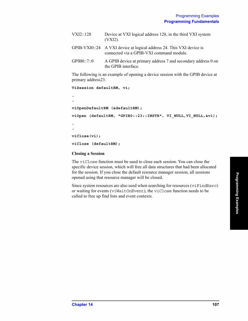
Programming ExamplesProgramming Fundamentals
Programm
ing Examples
VXI2::128 Device at VXI logical address 128, in the third VXI system (VXI2).
GPIB-VXI0::24 A VXI device at logical address 24. This VXI device is connected via a GPIB-VXI command module.
GPIB0::7::0 A GPIB device at primary address 7 and secondary address 0 on the GPIB interface.
The following is an example of opening a device session with the GPIB device at primary address23.
ViSession defaultRM, vi;
.
.
viOpenDefaultRM (&defaultRM);
viOpen (defaultRM, "GPIB0::23::INSTR", VI_NULL,VI_NULL,&vi);
.
.
viClose(vi);
viClose (defaultRM);
Closing a Session
The viClose function must be used to close each session. You can close the specific device session, which will free all data structures that had been allocated for the session. If you close the default resource manager session, all sessions opened using that resource manager will be closed.
Since system resources are also used when searching for resources (viFindRsrc) or waiting for events (viWaitOnEvent), the viClose function needs to be called to free up find lists and event contexts.
Chapter 14 107

Programming ExamplesProgramming Fundamentals
Prog
ram
min
g Ex
ampl
es
108 Chapter 14

Index
Index
AACP (ACLR) measurement, 15
View/Display key, 17, 18angle parameter (variables), 123arbitrary block data, 124
Bbit_pattern parameter (variables), 123block data
arbitrary, 124identifying block size, 124parsing output, 124
boolean parameter (commands), 122
CC language
addressing sessions, 136closing sessions, 137compiling and linking, 132creating, 131example, 133opening session, 134sessions, 135using VISA library, 131using VISA transition library, 132,
134channel power
advanced menu, 95channel bandwidth, 95power spectral density, 95
Channel Power keyMeas key, 13
channel power measurement, 11code domain
code domain with quad view, 97demodulated bit stream, 97I/Q error with quad view, 97I/Q gain imbalance, 96I/Q modulation impairments, 96I/Q quadrature error, 96in-channel characteristics, 96OVSF channels, 96
paging channel, 96pilot channel, 96sync channel, 96traffic channel, 96
power composite view, 96power graph & metrics, 97width of channel, 96
Code Domain (Quad View) keyView/Display key, 44, 48, 50
Code Domain keyMeas key, 39, 40, 48View/Display key, 42, 43, 44, 45,
46, 48, 49, 50, 51, 52, 60, 64commands
boolean parameter, 122keyword parameter, 122multiple on a line, 124parameters, 122syntax, 120termination, IEEE, 125units parameter, 122valid commands, 120variable parameter, 122variable parameter keywords, 122
complex spectrum measurementresults, 77
copyrights, 2
Ddata
arbitrary blocks, 124degree parameter (variables), 123Demod Bits key
View/Display key, 45, 51Device key
Radio key, 13
Ffrequency parameter (variables), 123
II/Q Error (Quad View) key
View/Display key, 42, 43, 49, 58, 59, 63, 72
I/Q Measured Polar Constln keyView/Display key, 58, 63, 72
IEEE command termination, 125instrument mode, 8integer variable (variables), 123
Kkeyword parameter (commands), 122
Llicenses, 2
MMeas key
Channel Power key, 13Code Domain key, 39, 40, 48Mod Accuracy (Composite EVM)
key, 57, 62Occupied BW key, 35Power Stat CCDF key, 67, 68QPSK EVM key, 71Spectrum Emission Mask key, 23,
24Spurious Emission key, 29
measurement
ACP or spurious emissions mask, 110
channel power, 95code domain, 96modulation accuracy (composite
rho), 98correlated power, 98error vector magnitude, 98frequency error, 98I/Q origin offset, 98magnitude error, 98modulation quality, 98number of active channels, 99peak code domain error, 98phase error, 98rho, 98time offset, 99
occupied bandwidth, 100spectrum shape, 100transmitter operation, 100
power statistics CCDF, 101Gaussian distribution curve, 103
QPSK EVM, 104phase and frequency quality, 104
QPSK EVM phase trajectory, 107spectrum emission mask, 109
measurement presets, 8measurement results
spurious emissions, 29measurement set up, 8measurements
ACP, 15channel power, 11increasing speed, 127spurious emissions, 27
measuring in the time domain, 82Mod Accuracy (Composite EVM) key
Meas key, 57, 62View/Display key, 58, 63
Mode keyW-CDMA with HSDPA/HSUPA
key, 13Mode Setup key
Radio key, 13W-CDMA with HSDPA/HSUPA
key, 13
Ooccupied bandwidth
99.0% bandwidth, 100Occupied Bandwidth measurement, 33Occupied BW key
Meas key, 35output data, identifying block size, 124
Pparameter (variables), 123
139
Index
Inde
x
parameters (commands), 122parameters, variable, 123percent parameter (variables), 123phase parameter (variables), 123power parameter (variables), 123Power Stat CCDF key
Meas key, 67, 68procedure
using the waveform measurement, 82
programmingcommand parameters, 122command syntax, 120example using C language, 133SCPI basics, 120using C language, 131valid commands, 120
QQPSK EVM
quadrature phase shift keying modulation, 104
QPSK EVM keyMeas key, 71View/Display key, 72
RRadio key
Device key, 13Mode Setup key, 13
relative power parameter (variables), 123
results data, identifying block size, 124results, waveform measurement, 111
SSCPI language
basic info, 120command parameters, 122command syntax, 120keyword parameters, 122valid commands, 120
signal connection, 8Spectrum (Frequency Domain) key,
108spectrum emission mask
reference channel integration bandwidth
method, 109spectral regrowth, 109spurious emission, 109
Spectrum Emission Mask keyMeas key, 23, 24
Spectrum Emission Mask measurement, 21
Spectrum key
View/Display key, 17, 18spectrum measurement
method, 108results, 77
Spurious Emission keyMeas key, 29
Spurious Emissionsmeasurement results, 29
spurious emissions measurement, 27spurs
measurement results, 29string parameter (variables), 123
Tthroughput, improving, 127time domain measurements, 111time parameter (variables), 123trace data format, 124triggering setup help, waveform
measurement, 82
Uunits parameter (commands), 122
Vvariable parameter (commands), 122variables
angle parameter, 123bit_data parameter, 123degree parameter, 123frequency parameter, 123integer parameter, 123parameters, 123percent parameter, 123phase parameter, 123power parameter, 123relative power parameter, 123string parameter, 123time parameter, 123voltage parameter, 123
View/Display keyACP (ACLR) measurement, 17, 18Code Domain (Quad View) key, 44,
48, 50Code Domain key, 42, 43, 44, 45,
46, 48, 49, 50, 51, 52, 60, 64Demod Bits key, 45, 51I/Q Error (Quad View) key, 42, 43,
49, 58, 59, 63, 72I/Q Measured Polar Constln key, 58,
63, 72Mod Accuracy (Composite EVM)
key, 58, 63QPSK EVM key, 72Spectrum key, 17, 18
view/display selection
I/Q Waveform view, 82magnitude & phase graph view, 82
viewing the time domain, 82VISA library, 132, 134voltage parameter (variables), 123VTL, compiling and linking C
language, 132
Wwaveform
method, 111Waveform (Time Domain) key, 111waveform measurement, 82
results, 81W-CDMA with HSDPA/HSUPA key
Mode key, 13Mode Setup key, 13
140