CCSS Grade 7 TV V1.1 - CPM Educational Program

Making Connections: Course 2 (Grade 7) Supplemental Materials, V1.1 i

Making Connections: Course 2 CCSS Grade 7 Supplemental Materials Teacher Edition, Version 1.1 Supplement to CPM Making Connections, Course 2 This booklet supplements the CPM Educational Program textbook, Making Connections: Foundations for Algebra, Course 2. Together, these two publications align with the Common Core State Standards for Grade 7 (Standards for Mathematical Practice and Standards for Mathematical Content). Managing Editor Bob Petersen Sacramento, CA

Contributing Editors Scott Coyner Sacramento, CA

Leslie Dietiker Michigan State University

Lori Hamada Fresno, CA

Brian Hoey Sacramento, CA

Michael Kassarjian Dallas, TX

Judy Kysh San Francisco, CA

Sarah Maile Sacramento, CA

Technical Manager

Sarah Maile Sacramento, CA Program Directors Leslie Dietiker Judy Kysh, Ph.D. Michigan State University Departments of Mathematics and Education East Lansing, MI San Francisco State University Brian Hoey Tom Sallee, Ph.D. Christian Brothers High School Department of Mathematics Sacramento, CA University of California, Davis

Making Connections: Course 2 (Grade 7) Supplemental Materials, V1.1 ii

Copyright © 2011 by CPM Educational Program. All rights reserved. No part of this publication may be reproduced or transmitted in any form or by any means, electronic or mechanical, including photocopy, recording, or any information storage and retrieval system, without permission in writing from the publisher. Requests for permission should be made in writing to: CPM Educational Program, 1233 Noonan Drive, Sacramento, CA 95822. Email: [email protected].

1 2 3 4 5 6 7 8 9 15 14 13 12 11

Printed in the United States of America ISBN 78-1-60328-061-7

Making Connections: Course 2 (Grade 7) Supplemental Materials, V1.1 iii

Making Connections: Course 2 CCSS Grade 7 Supplemental Materials

Teacher Edition, Version 1.1

Supplement to CPM Making Connections, Course 2

This booklet supplements the CPM Educational Program textbook, Making Connections: Foundations for Algebra, Course 2. Together, these two publications align with the Common Core State Standards for Grade 7 (Standards for Mathematical Practice and Standards for Mathematical Content). This supplemental booklet is available for download for no charge at http://www.cpm.org/teachers/CCSS_Supplements.htm. A correlation of the CCSS Grade 7 content standards with these two publications is available at www.cpm.org/teachers/CCSS_Correlations.htm. A correlation of the CCSS mathematical practices with these two publications is available at http://www.cpm.org/teachers/CCSS_Practices.htm.

CCSS Grade 7 Supplemental Topics

Angle Pairs 1 For use after MC2* Chapter 9 Statistics and Probability Resource: Unit 3 5 For use after MC2 Lesson 11.2.4 Statistics and Probability Resource: Lesson 2.2.2 39 For use after MC2 Lesson 11.2.4 * “MC2” refers to CPM Making Connections: Foundations for Algebra, Course 2

Making Connections: Course 2 (Grade 7) Supplemental Materials, V1.1 iv

Possible Sequence of a CCSS-Aligned CPM Grade 7 Course This supplemental book contains lessons that should be inserted into the usual flow of the CPM course, Making Connections: Foundations for Algebra, Course 2. The Table of Contents that follows (from CPM Making Connections: Foundations for Algebra, Course 2) suggests where these supplemental lessons can be inserted into the course. In addition, suggestions are offered as to which material in the CPM text can be skipped. By following this suggested sequence, both the CCSS content standards and the CCSS practice standards will be fully addressed. Lessons in the Table of Contents that follows are listed as “necessary,” “suggested,” or “optional.” “Necessary” lessons are lessons that are required to align with the Common Core State Standards for Mathematics for Grade 7 Mathematical Content. “Suggested” lessons will enhance learning and provide coherence. “Optional” lessons cover standards from previous or subsequent CCSS courses. It is not suggested nor is it desirable to skip all of the optional lessons, as some may be beneficial for introducing or refreshing the elements of effective student work using study teams. Additionally, selective optional lessons may be chosen at the teacher’s discretion to refresh skills that were taught the previous year or to preview upcoming material. However, since there is substantial new material encompassed in the necessary and suggested lessons, and because students will continually review previous and new material throughout the course, teachers are advised to be cautious not to spend too many days with the optional lessons found in the first few chapters. Chapter 1 Probability and Portions Section 1.1 Course Introduction Problems 1.1.1 Finding Shared and Unique Characteristics suggested 1.1.2 Perimeter and Area Relationships suggested 1.1.3 Finding Unknowns suggested 1.1.4 Representing Data suggested 1.1.5 Investigating Number Patterns necessary

Section 1.2 Probability 1.2.1 Exploring Probability necessary 1.2.2 Comparing Experimental and Theoretical Probabilities necessary 1.2.3 Rewriting Fractions necessary 1.2.4 Compound Probability and Fraction Addition necessary 1.2.5 Subtracting Fractions necessary

Section 1.3 Relating Fractions and Decimal 1.3.1 Fraction to Decimal Conversions necessary 1.3.2 Rewriting Decimals as Fractions necessary Chapter Closure necessary Puzzle Investigator Problems optional

Making Connections: Course 2 (Grade 7) Supplemental Materials, V1.1 v

Chapter 2 Transformations and Area Section 2.1 Integer Operations 2.1.1 Adding Positive and Negative Numbers necessary 2.1.2 Adding and Subtracting Integers necessary 2.1.3 More Integer Operations necessary

Section 2.2 Introduction to Transformations 2.2.1 Rigid Transformations optional (grade 8) 2.2.2 Rigid Transformations on a Coordinate Grid optional (grade 8) 2.2.3 Describing Transformations optional (grade 8) 2.2.4 Multiplication and Dilation necessary Extension Activity: Using Rigid Transformations optional

Section 2.3 Area 2.3.1 Multiplication of Fractions necessary 2.3.2 Decomposing and Recomposing Area necessary 2.3.3 Area of Parallelograms optional (grade 6) 2.3.4 Area of Triangles optional (grade 6) 2.3.5 Area of Trapezoids optional (grade 6) 2.3.6 Order of Operations necessary

Chapter Closure necessary Puzzle Investigator Problems optional Chapter 3 Building Expressions Section 3.1 Variables and Expressions 3.1.1 Area of Rectangular Shapes necessary 3.1.2 Naming Perimeters of Algebra Tiles necessary 3.1.3 Combining Like Terms necessary 3.1.4 Evaluating Variable Expressions necessary 3.1.5 Perimeter and Area of Algebra Tile Shapes necessary

Section 3.2 Solving Word Problems 3.2.1 Describing Relationships Between Quantities necessary 3.2.2 Solving a Word Problem necessary 3.2.3 Strategies for Using the 5-D Process necessary 3.2.4 Using Variables to Represent Quantities in Word Problems necessary 3.2.5 More Word Problem Solving necessary

Chapter Closure necessary

Puzzle Investigator Problems optional

Making Connections: Course 2 (Grade 7) Supplemental Materials, V1.1 vi

Chapter 4 Proportional Reasoning and Statistics Section 4.1 Percents 4.1.1 Part-Whole Relationships necessary 4.1.2 Finding and Using Percentages necessary

Section 4.2 Analyzing Data 4.2.1 Measures of Central Tendency necessary 4.2.2 Multiple Representations of Data necessary 4.2.3 Analyzing Box-and-Whisker Plots necessary 4.2.4 Comparing and Choosing Representations necessary

Section 4.3 Similarity 4.3.1 Dilations and Similar Figures optional (grade 8) 4.3.2 Identifying Similar Shapes optional 4.3.3 Working With Corresponding Sides optional 4.3.4 Solving Problems Involving Similar Shapes optional

Chapter Closure necessary Puzzle Investigator Problems optional Chapter 5 Inequalities and Descriptive Geometry Section 5.1 Writing Expressions 5.1.1 Inverse Operations necessary 5.1.2 Translating Situations into Algebraic Expressions necessary 5.1.3 Simplifying Algebraic Expressions necessary

Section 5.2 Solving Inequalities 5.2.1 Comparing Expressions necessary 5.2.2 Comparing Quantities with Variables necessary 5.2.3 One Variable Inequalities necessary 5.2.4 Solving One Variable Inequalities necessary

Section 5.3 Circles and Descriptive Geometry 5.3.1 Introduction to Constructions necessary 5.3.2 Compass Constructions necessary 5.3.3 Circumference and Diameter Ratios necessary 5.3.4 Circle Area necessary

Section 5.4 Mid-Course Reflection 5.4.1 Mid-Course Reflection Activities optional Chapter Closure necessary Puzzle Investigator Problems optional

Making Connections: Course 2 (Grade 7) Supplemental Materials, V1.1 vii

Chapter 6 Graphing and Solving Equations Section 6.1 Correlations, Predictions and Linear Functions 6.1.1 Circle Graphs optional 6.1.2 Organizing Data in a Scatterplot optional (grade 8) 6.1.3 Identifying Correlation optional (grade 8) 6.1.4 Introduction to Linear Rules optional (grade 8) 6.1.5 Intercepts optional (grade 8) 6.1.5 Tables, Linear Graphs, and Rules optional (grade 8) Extension Activity: Finding and Describing Relationships optional (grade 8) Section 6.2 Writing and Solving Equations 6.2.1 Solving Equations necessary 6.2.2 Checking Solutions and the Distributive Property necessary 6.2.3 Solving Equations and Recording Work necessary 6.2.4 Using a Table to Write Equations from Word Problems necessary 6.2.5 Writing and Solving Equations necessary 6.2.6 Cases with Infinite or No Solutions optional (grade 8) 6.2.7 Choosing a Solving Strategy necessary Chapter Closure necessary Puzzle Investigator Problems optional Chapter 7 Slopes and Rates of Change Section 7.1 Ratios, Rates, and Slope 7.1.1 Comparing Rates necessary 7.1.2 Comparing Rates with Graphs and Tables necessary 7.1.3 Unit Rates necessary 7.1.4 Slope optional (grade 8) 7.1.5 Slope in Different Representations optional (grade 8) 7.1.6 More About Slope optional (grade 8) Section 7.2 Systems of Equations 7.2.1 Systems of Equations optional (grade 8) 7.2.2 Solving Systems of Equations optional (grade 8) 7.2.3 More Solving Systems of Equations optional (grade 8) Chapter Closure optional Puzzle Investigator Problems optional

Making Connections: Course 2 (Grade 7) Supplemental Materials, V1.1 viii

Chapter 8 Percents and More Solving Equations Section 8.1 Distance, Rate, and Time 8.1.1 Distance, Rate, and Time necessary 8.1.2 Comparing Rates necessary

Section 8.2 Percent Increase and Decrease 8.2.1 Scaling Quantities necessary 8.2.2 Solving Problems Involving Percents necessary 8.2.3 Equations with Fraction and Decimal Coefficients necessary 8.2.4 Creating Integer Coefficients necessary 8.2.5 Percent Increase and Decrease necessary 8.2.6 Simple Interest necessary Chapter Closure necessary Puzzle Investigator Problems optional Chapter 9 Proportions and Pythagorean Theorem Section 9.1 Solving Proportions 9.1.1 Recognizing Proportional Relationships necessary 9.1.2 Proportional Equations necessary 9.1.3 Solving Proportions necessary

Section 9.2 Ratio of Areas 9.2.1 Area and Perimeter of Similar Shapes optional 9.2.2 Growth Patterns in Area optional 9.2.3 Applying the Ratio of Areas optional

Section 9.3 Pythagorean Theorem 9.3.1 Side Lengths and Triangles necessary 9.3.2 Pythagorean Theorem optional (grade 8) 9.3.3 Understanding Square Root optional (grade 8) 9.3.4 Applications of the Pythagorean Theorem optional (grade 8) Grade 7 CCSS Supplement: Angle Pairs necessary Chapter Closure optional Puzzle Investigator Problems optional

Making Connections: Course 2 (Grade 7) Supplemental Materials, V1.1 ix

Chapter 10 Exponents and Three Dimensions Section 10.1 Interest and Exponent Rules 10.1.1 Patterns of Growth in Tables and Graphs optional (grade 8) 10.1.2 Compound Interest optional 10.1.3 Linear and Exponential Growth optional (grade 8) 10.1.4 Exponents and Scientific Notation optional (grade 8) 10.1.5 Exponent Rules optional (grade 8) 10.1.6 Negative Exponents optional (grade 8) Section 10.2 Surface Area and Volume 10.2.1 Surface Area and Volume necessary 10.2.2 Visualizing Three-Dimensional Shapes necessary 10.2.3 Volume of a Prism necessary 10.2.4 Volume of Non-Rectangular Prisms necessary 10.2.5 Surface Area and Volume of Cylinders optional (grade 8) 10.2.6 Volume of Cones and Pyramids optional (grade 8) Chapter Closure optional Puzzle Investigator Problems optional Chapter 11 Growth, Probability, and Volume Section 11.1 Non-Linear Growth 11.1.1 Non-Linear Growth optional (grade 8) 11.1.2 Absolute Value optional (grade 8) Section 11.2 More Probability 11.2.1 Revisiting Probability necessary 11.2.2 Comparing Probabilities necessary 11.2.3 Modeling Probabilities of Compound Events necessary 11.2.4 Compound Events necessary Grade 7 CCSS Supplement: Statistics and Probability: Unit 3 necessary Grade 7 CCSS Supplement: Statistics and Probability: Lesson 2.2.2 necessary Section 11.3 Scale Factor and Volume 11.3.1 Exploring Volume optional 11.3.2 Scale Factor and Volume optional 11.3.3 More Scale Factor and Volume optional Section 11.4 Closure Problems and Activities 11.4.1 Indirect Measurement optional 11.4.2 Representing and Predicting Patterns optional 11.4.3 Volume and Scaling optional 11.4.4 Analyzing Data to Identify a Trend optional Chapter Closure optional Puzzle Investigator Problems optional

Making Connections: Course 2 (Grade 7) Supplemental Materials, V1.1 1

ANGLE PAIRS

NAMES AND PROPERTIES OF ANGLE PAIRS

It is common to identify angles using three letters. For example, !ABC means the angle you would find by going from point A to point B to point C in the diagram at right. B is the vertex of the angle (where the endpoints of the two sides meet) and BA

! "!! and

BC! "!!

are the rays that define it. A ray is a part of a line that has an endpoint (starting point) and extends infinitely in one direction.

If two angles have measures that add up to 90°, they are called complementary angles. For example, in the diagram above right, !ABC and !CBD are complementary because together they form a right angle.

If two angles have measures that add up to 180°, they are called supplementary angles. For example, in the diagram at right, !EFG and !GFH are supplementary because together they form a straight angle.

Two angles do not have to share a vertex to be complementary or supplementary. The first pair of angles at right are supplementary; the second pair of angles are complementary.

Adjacent angles are angles that have a common vertex, share a common side, and have no interior points in common. So angles ! c and ! d in the diagram at right are adjacent angles, as are ! c and ! f, ! f and ! g, and ! g and ! d.

Vertical angles are the two opposite (that is, non-adjacent) angles formed by two intersecting lines, such as angles ! c and ! g in the diagram above right. ! c by itself is not a vertical angle, nor is ! g, although ! c and ! g together are a pair of vertical angles. Vertical angles always have equal measure.

C A

B D

F H E

G

60°

120° 40°

50°

Supplementary Complementary

c d f

g


s 30°

ANGLE PAIRS AND EQUATIONS Based on the above information, equations may be written and then solved. Example 1 These angles are complementary. s + 30º= 90º

s = 60º

Example 2 These angles are vertical. 2x + 2 = 30º

2x = 28ºx = 14º

Example 3 These angles are supplementary. x + 6 + 4x !1 = 180º

5x + 5 = 180º5x = 175ºx = 35º

Example 4 These 3 angles are adjacent and together total 43º . x + x + 23º= 43º2x + 23º= 43º

2x = 20ºx = 10º

x x

23° 43°

30º

2x + 2

x + 6 4x – 1


135°

4k–5

40!

3x –5

Problems Based on the information in each diagram, write and solve an equation for the variable. 1.

2.

3.

4.

5.

6.

7.

8.

9.

10.

11.

12.

55˚

90˚

5k

12 x

12 x

x

140°

x

x x

36˚ 90˚

2x 60°

2m + 4

30°

b c

115° a

t

w

2x – 6 4x – 12

x

120° 45°

135°

5w

z


Answers 1. x = 15 2. x = 60 3. m = 28 4.!!!!!!a = c = 65

b = 115

5. t = w = 90

6. x = 33 7. k = 35 8. x = 70

9.!!!!!!w = 27!!!!!!!!!!z = 45

10. x = 90 11. k = 7 12. x = 18


Unit 3 Comparing One-Variable Samples


Unit 3 Teacher Guide

Section Lesson Days Lesson Title Materials Core Problems

3.1.1 2 Measurement Precision

• Rulers • Measuring tapes

3-1 to 3-4 and

3-5 to 3-6 3.1

3.1.2 1 Comparing Distributions None 3-13 to 3-15

3.2.1 1 Representative Samples None 3-19 to 3-23

3.2 3.2.2 1 Inference from

Random Samples

• Envelopes • Scissors • Lesson 3.2.2 Res. Pg.

3-26, 3-27, and 3-29

Total: 5 days


Overview of Unit

This unit builds on the single-variable data displays from Unit 1. Students begin the unit by comparing distributions of data collected from two measurement tools. They conclude that using a tape measure to measure large distances is more precise than using a ruler. This leads to the second lesson in which distributions of data are further compared. Students quantify the overlap in two distributions by using the IQR as a benchmark: the difference between two medians is expressed as a multiple of the IQR.

In Section 3.2, students explore how data is collected. They learn what a representative sample of a population is and learn that random samples are a good way to collect representative data. Students then make inferences about the population from samples. Finally, students informally determine intervals for which characteristics of the population fall. Standards

Common Core State Standards: 7.SP 1. Understand that statistics can be used to gain information about a population by

examining a sample of the population; generalizations about a population from a sample are valid only if the sample is representative of that population. Understand that random sampling tends to produce representative samples and support valid inferences.

7.SP 2. Use data from a random sample to draw inferences about a population with an unknown characteristic of interest. Generate multiple samples (or simulated samples) of the same size to gauge the variation in estimates or predictions. For example, estimate the mean word length in a book by randomly sampling words from the book; predict the winner of a school election based on randomly sampled survey data. Gauge how far off the estimate or prediction might be.

7.SP 3. Informally assess the degree of visual overlap of two numerical data distributions with similar variabilities, measuring the difference between the centers by expressing it as a multiple of a measure of variability. For example, the mean height of players on the basketball team is 10 cm greater than the mean height of players on the soccer team, about twice the variability (mean absolute deviation) on either team; on a dot plot, the separation between the two distributions of heights is noticeable.

7.SP 4. Use measures of center and measures of variability for numerical data from random samples to draw informal comparative inferences about two populations. For example, decide whether the words in a chapter of a seventh-grade science book are generally longer than the words in a chapter of a fourth-grade science book.

NCTM Principles and Standards:

Use observations about differences between two or more samples to make conjectures about the populations from which the samples were taken.


About the Problems

The “core problems” in a lesson are identified in the teacher notes preceding each lesson. The core problems are designed to meet the lesson objectives. Additional problems are provided for students to practice individually. These problems can be assigned as homework or classwork to give students the opportunity to process the learning individually. These additional problems review the lesson objectives for that particular lesson, but do not typically go back and review materials from previous lessons or previous units. Prerequisites

This unit assumes that students have completed, Unit 1: Describing One-Variable Data of this CPM Statistics and Probability Resource. Alternatively students should have learned standards 6.SP1 through 6.SP5 of the Common Core State Standards for High School Statistics and Probability elsewhere. Specifically, students come prepared for this unit being able to describe the distribution of a set of data using center, shape, spread, and outliers. Students can display a distribution using a dot plot, histogram, and box plot. Students can also give quantitative measures of center (median and/or mean) and variability (interquartile range and/or mean absolute deviation). Technology

It is expected that students will have their scientific calculators available at all times, including for any additional problems you may assign for homework. Effective Teamwork

This unit is designed for students to explore mathematics in study teams. Lessons and problems throughout the unit have been constructed with the expectation that students will work together and be able to discuss ideas as they are developed. Team learning is one of the three research-based principles of CPM courses that foster long-term learning. (The complete research base for CPM courses is described at www.cpm.org/teachers/research.htm.) Collaboration will allow students to develop new ways of thinking about mathematics, increase students’ abilities to communicate with others about math, and help them strengthen their understanding by having to explain their thinking to someone else. Students are expected to work in teams for the majority of class time, so it is imperative for teams to function well. For suggestions about how to set up effective teams, refer the “Using Study Teams for Effective Learning” section in the teacher edition of any of the CPM Connections courses or at the CPM website: www.cpm.org/teachers/study.htm.


Lesson 3.1.1 Which tool is more precise? Measurement Precision Lesson Objective: Students will measure a length using two different measuring tools and

generate two sets of data. They will then compare the data by creating histograms and box plots to analyze center, shape, spread, and outliers. Students will begin to develop the understanding that the fewer iterations of a tool that are needed, the more precise the measurement is likely to be.

Standards: CCSS: 7.SP 3. Informally assess the degree of visual overlap of two numerical data distributions with similar variabilities, [measuring the difference between the centers by expressing it as a multiple of a measure of variability.] NCTM: Use observations about differences between two or more samples to make conjectures about the populations from which the samples were taken.

Length of Activity: Two days (approximately 90 minutes)

Core Problems: Day One: Problems 3-1 through 3-4 Day Two: Problems 3-5 and 3-6

Materials: 12-inch rulers, one per student Measuring tapes that are long enough to span one dimension of the classroom, one per team

Materials Preparation:

Before class, decide what length you will have students measure. Many teachers use a span of their classroom. Other options might be the width of a basketball court, tennis court, or other athletic facility, a hallway, or the entire school building. Note: If your classroom floor is tiled with 12-inch tiles, choose a different length for the students to measure. Whatever the length you choose, be sure you have a relatively precise measurement yourself so that you have an idea of the measurements you expect the students to find.

Suggested Lesson Activity:

Day One: Being by having a student volunteer read the lesson introduction and focus questions. Then move on to problem 3-1, which asks students to predict how the data obtained by measuring a length twice with two different measuring tools might compare. Use the questions to lead a whole-class discussion about what the students


think will happen. Then prepare them to begin the task by having a volunteer read problem 3-2 aloud. Before you distribute the 12-inch rulers and measuring tapes, be sure to clarify which length students are measuring, and make suggestions about how several students can measure at once. Remind students that it is important to have every student measure with each tool, since the class will need the data from each of these measurements to compare the tools. If the students think that once they measure they will use that same measurement for the other tool, they are undermining the nature of the experiment. Emphasize that for the experiment to be valid, the data must be gathered as carefully and methodically as possible. To help with time management, teams that finish early should work on problem 3-3, which asks them to analyze the data just from their team. Teams that finish later can skip this question or return to it later. Note: If you choose not to have students actually measure, you can use the sample data for the length of a particular classroom at right. Once all of the data is collected, have teams move on to problem 3-4. Have students record their measurements in a table on the whiteboard or overhead projector so that the whole class can see them. (As students post data, monitor to ensure that each measurement ends up on the correct poster.) After teams have had a few minutes to work on part (b), pull the class together for a whole-class discussion about their ideas on possible outliers. Obvious errors should be corrected or deleted. Part (c) of this problem is preparing students for creating histograms and box plots tomorrow. If you have time, feel free to have students start on tomorrow’s lesson. Note: Direct students to put their work from today in a safe place, as they will use it for the next day. You may want to analyze the data yourself overnight so that you can help students with the intervals on their histograms tomorrow. See the first two paragraphs for Day Two below. Day Two: In part (a) of problem 3-5 students will be making a histogram and in part (b) they will make a box plot. The amount of time it takes to complete this problem, and how much review and guidance you will need to provide, will depend on how experienced

Measures with Ruler

Measures with Tape

324 334 337 343 317 346

330 312 334 320 328 341

335 341 334 340 338 345

330 329 319 321

334 337 330 336 335 335

339 340 336 341 338 340

336 340 338 337 334 339

336 341 337 336


your students are with creating histograms and box plots and describing their characteristics (Unit 1 of this CPM Statistics and Probability Resource).

You may need to assist students with selecting a bin width (interval size) to display the data nicely in the histogram. This goes much more smoothly if you have reviewed the data yourself in advance. As a very broad guideline, some teachers use the square root of the number of observations as the number of bins. For the sample data given, a scale from 310 to 350 with a bin width (interval size) of 5 will work well.

Part (c) of problem 3-5 then asks students to compare the two distributions of data using center, shape, spread, and outliers. Expect a wide variety of observations, related to particular values, the minimum and maximum values, etc. To elicit observations about spread (variability), ask, “Does the data make the same shape in each histogram?” and “Do you notice that this histogram is much taller and thinner while this is shorter and more spread out? What does that say about the data?” Obviously comparisons will vary based on the actual data students collect, but some possible comparisons are given in the solution to the problem. Then direct teams to discuss problem 3-6, in which they will choose a particular measurement as the length of the classroom. Give teams a chance to share their reasoning. Pull the class together and ask questions about the point of this activity. Some possible questions include, “What was the point of this study?”, “How did organizing the data give you a better sense of the measures we found as a class?”, “Which tool seemed to give more consistent measures? How can you tell?”, and “Why didn’t everyone get the same measures?”

Closure: (5 minutes)

Direct teams to discuss problem 3-7, and then pull the class together for a brief discussion. Students are likely to think creatively about ways to obtain a perfect measurement. Encourage these ideas, but be sure that students understand that all measurements are approximate, although, as this lesson has demonstrated, some tools are more likely to lead to more precise approximations than others.

Additional Problems:

Day One: Problems 3-8 and 3-9 Day Two: Problems 3-10 through 3-12


3.1.1 Which tool is more precise? • • • • • • • • • • • • • • • • • • • • • • • • • • • • • • • • • • • • • • • • • • • • • • • • • • • • • • • • • • • • • • • • • Measurement Precision Does the tool that you use matter when you measure length? Do the lengths of the object you are measuring or the tool you choose to measure with affect how precise your measurement is likely to be? In this section, your class will explore this question by analyzing the results of an experiment. As you work with your team, think about the following questions:

What am I measuring?

What unit is being iterated?

What can I do to make my measurement more precise? 3-1. WHICH TOOL GIVES A MORE PRECISE MEASUREMENT? Have you heard the expression, “Measure twice, cut once”? This advice refers to the

care that professionals such as carpenters and fashion designers need to take to measure precisely so that all of the parts of their creations fit together correctly. Does it matter what tool they use to make their measurements?

Imagine using two different tools, such as a 12-inch ruler and a continuous measuring

tape, to measure a length of your classroom or the width of a basketball court (in inches). How might the measurements that you get compare?

Discuss the following questions with your team. Be prepared to share your ideas with

the rest of the class.

• Would you get the same measurement with each tool? • Why might the measures be different? Should they be the same? • Which tool do you think would give you a more precise measurement?

That is, one that is closer to the true length of the classroom?


3-2. Now you and your class will gather data to test your ideas about the precision of measuring the same length with two different tools.

Your task: As directed by your teacher, measure the described length to the nearest

inch twice, each time using a different tool (a 12-inch ruler and a single measuring tape, for example). Although you will share tools with your team and work together to make sure the measures are recorded properly, each person in the team should measure the length twice, once with each tool.

3-3. Once your team members have each made their measurements, compare the results

within your team by answering the following questions:

• Which tool seems to measure more precisely? • What do you think is the actual length of the classroom? How did

you decide? • Which tool do you think gave you a better answer?

3-4. Add your data to the class data table.

a. Examine the sets of data. Record any initial observations you can make.

b. Are there any measures that look very different from the others? These extreme values are called outliers. What could you do to help you see any outliers better? [ Sort the data into order. Plotting the data will also help; this will be done in the next problem. ]

c. Sometimes an outlier can reveal that an error or misunderstanding has occurred. Decide as a class if any data needs to be deleted or corrected due to an error or misunderstanding. [ Answers vary. ]

d. What is the range for each set of data? How do the ranges compare? For each set of data, what is the median? What is the first quartile? The third quartile? [ Answers vary. ]


3-5. Creating visual representations of data makes data sets easier to compare.

a. Make a histogram for each set of data. Make sure to use the same scale for both histograms. [ See histograms below for the sample data. ]

b. Create parallel box plots for the two sets of data, using the same scale as for your histogram. [ If you are using the sample data, the parallel box plot is shown at right. ]

c. Compare the center, shape, spread, and outliers for the two sets of data using the histograms and the box plots. Do they seem to show the same value for the length of the classroom? [ The median with the tape measure is slightly higher, but considering the spread, the difference in medians is not very noteworthy. Both distributions are symmetric, single-peaked, and mound-shaped. There is much more variability in the measurements with the ruler; the tape measure is much more consistent. There are no apparent outliers for the rulers; 330 might be an outlier for the tape measures since the variability of the tape measures is so narrow. ]

320 330 340 350 Length (in inches) from

Measuring Tape

Freq

uenc

y

Length (in inches) from Rulers

Freq

uenc

y

310 320 330 340 350

320 330 340 350 310


3-6. WHICH MEASUREMENT IS BEST? So what is the actual measure? Clearly you

have multiple measurements from which to choose. How can you decide what is the best estimate of the length of the classroom?

Look at the data set for each tool, along with

their histograms and box plots, and consider the center, shape, spread, and outliers. With your team, discuss what you can learn from each of these pieces of information about the precision (consistency) of each measuring tool, as well as about the length of the classroom. Which of the many numbers that you could choose is the best estimate for the actual length of the classroom? Why? What do you think accounts for the greater consistency of one tool? [ While the answer varies depending on the data, the median of the measures with the measuring tape (which should have a smaller spread of data) is a good approximation. We expect students to notice that the measuring tape is more consistent because the measures have less spread (variability) since it avoids the error caused by picking up and moving the ruler. ]

3-7. IS MEASUREMENT ALWAYS APPROXIMATE? As you have seen, the measurements you took are approximate. Is this always true?

Can you imagine a way to measure something that would be exact without any variability? Discuss this with your team and be prepared to share your ideas with the class. [ Ideas vary, but students should conclude that all measurements are approximate. ]


3-8. Ms. Whitney has thirteen students who did extra-

credit assignments to raise their grades. The scores on the assignments were 96, 45, 89, 100, 100, 77, 67, 84, 98, 33, 60, 97, and 100.

a. Make a stem-and-leaf plot of this data. [ See diagram at right. ]

b. Find the median, and the first and third quartiles. [ Median = 89, Q1 = 63.5, Q3 = 99 ]

3-9. Mrs. Ferguson, your school librarian, asks you to conduct

a survey of how many books students read during the year. You get the following results: 12, 24, 10, 32, 12, 4, 35, 10, 8, 12, 15, 20, 18, 25, 21, and 9.

a. Use the data to create a histogram. Use a bin width of 10 books. [ See plot at right. ]

b. Is the mean or median a better measure of the center? Find the value of whichever is more appropriate. [ The data is nearly symmetric with no outliers so either mean or median are appropriate. Mean = 16.69 books, median = 13.5 books ]

c. Make a box plot of the data. [ See box plot at right. ]

d. Describe the center, shape, spread, and outliers of the distribution. [ The typical student reads about 13.5 books. The distribution is nearly symmetrical, single-peaked, and mound-shaped. Some students may say there is a slight right skew, apparent in the box plot. The IQR is 12.5 so there is a lot of variability in the number of books read. There are no apparent outliers. ]

Additional Problems

Note: 2 1 means 21

3 3 4 5 5 6 0 7 7 7 8 4 9 9 6 7 8

10 0 0 0

0 10 20 30 40

0 10 20 30 40


3-10. Ms. Carpenter asked each of her students to record how much time it takes them to get from school to home this afternoon. The next day, students came back with this data, in minutes: 15, 12, 5, 55, 6, 9, 47, 8, 35, 3, 22, 26, 46, 54, 17, 42, 43, 42, 15, 5.

a. Create a combination histogram and box plot to display this information. Use a bin width of 10 minutes. [ See histogram and box plot at right. ]

b. Find the mean and the median. Why does neither plot seem very adequate in describing the center of this distribution? How could you better describe a “typical” trip home? [ The mean is 25.35, the median is 19.5 minutes. The distribution is bimodal; the measures of center fall between the peaks. Typical times seem to center around 10 minutes and 45 minutes. ]

c. Considering the context, make a conjecture as to why this data has a bimodal shape. [ There are two groups of students. Possibly some walk home and others take the bus, or perhaps the school serves two neighborhoods that are a distance apart. ]

3-11. The students at Dolan Middle School are competing

in after-school activities in which they earn points for helping out around the school. Each team consists of the 30 students in a homeroom. Halfway through the competition, here are the scores from the students in two of the teams.

The champion team is the one with the most points when the scores of the 30 students on the team are added. Which team would you rather be on? Explain. [ Both teams seem to be very even in total points. Team 1 is more consistent and has fewer very low scores, so it may be the better choice, even though Team 2 has a slightly higher median at this time. ]

Team 1 Team 2

0 10 20 30 40 50 60


3-12. Scientists studying prehistoric birds have estimated the weights (in grams) of two different sub-species of birds. The data they collected is shown below.

Pre-emergent Thrushes: 49, 54, 52, 58, 61, 72, 73, 78, 73, 82, 83, 73, 61, 67, 68

Post-emergent Thrushes: 65, 35, 48, 29, 57, 87, 94, 68, 86, 73, 58, 74, 85, 91, 88, 97

a. Create a parallel box plot to compare the weights of these two sub-species of birds. [ See parallel box plot at right. ]

b. Would the mean accurately represent the middle of the data? Why or why not? [ Yes. Both distributions are fairly symmetric with no apparent outliers. ]

c. A fossil of a bird is found. Scientists estimated that its weight must have been around 75 grams. Which sub-species was the bird most likely a member of? Explain. [ Post-emergent thrushes. More than 75% of the pre-emergent thrushes weighed less than 75 grams, so that is not a likely candidate. 75 grams is close to the median of post-emergent thrushes. ]

40 20 30 50 60 70 80 90 100


One way to visually represent a distribution of collected data is with a combination histogram and box plot. The box plot is graphed on the same x-axis as the histogram. See Alejandro’s scores at right.

To compare two distributions, a second combination histogram and box plot is drawn with the same scale as the first histogram. The two combination plots can then be lined up exactly on top of each other so that differences are readily observable. Compare Alejandro’s scores from above to César’s scores at right.

Sometimes comparing only the two box plots is enough to be able to compare the distributions. When two box plots are drawn on the same axis, they are called parallel box plots. An example is shown below.

0 1 2 3 4 5 6 7 8 9 10

Alejandro

César

ETHODS AND MEANINGS M

ATH

NO

TES Comparing Box Plots

0 1 2 3 4 5 6 7 8 9 10

Alejandro’s Scores

0 1 2 3 4 5 6 7 8 9 10

César’s Scores


Lesson 3.1.2 How can I compare the results? Comparing Distributions Lesson Objective: Students will compare two populations based on making inferences

from samples. Students will quantify the difference between the medians as a multiple of the IQR.

Standards: CCSS: 7.SP 3. Informally assess the degree of visual overlap of two numerical data distributions with similar variabilities, measuring the difference between the centers by expressing it as a multiple of a measure of variability. 7.SP 4. Use measures of center and measures of variability for numerical data from [random] samples to draw informal comparative inferences about two populations. NCTM: Use observations about differences between two or more samples to make conjectures about the populations from which the samples were taken.

Length of Activity: One day (approximately 45 minutes)

Core Problems: Problems 3-13 through 3-15

Materials: None


Start class with a summary of Lesson 3.1.1. Remind students that they drew conclusions by comparing the distributions of two sets of data. Remind students that the medians were very similar; what differed was the variability of the data which we related to the precision of the measuring tool. In problem 3-13, students are given the bin width for the histogram. At this point, do not expect students to be very good at choosing bin widths. By giving them bin widths they can concentrate on the analysis of the data. Students will become much more proficient at creating appropriate histograms in the high school units. In problem 3-13 students will notice that the medians are quite different from each other. However, in problem 3-14 students are led to the conclusion that this difference in means is not all that noteworthy, since it falls within the variability of one of the distributions. The difference in the medians in problem 3-15 is much more remarkable since the intervals of the IQR do not even overlap. In part (e) students will use the IQR to quantify how different the medians


really are from each other. If students are having a difficult time visualizing this, suggest to them to use the IQR interval like they would a ruler. We are counting how many “rulers” the medians are apart. Problem 3-16 gives students additional time to process using the IQR as a measure of the difference between medians. Students are given less guidance in this problem than they were in previous problems, and the medians are not as dramatically different as they were in the previous problem.


A lengthy closure is not required today. Verify that students understand what a parallel box plot is, and that a difference in medians becomes noteworthy only when it is compared to the width of the distribution. They can share their solutions to problem 3-16.


Problems 3-17 through 3-20


3.1.2 How can I compare the results? • • • • • • • • • • • • • • • • • • • • • • • • • • • • • • • • • • • • • • • • • • • • • • • • • • • • • • • • • • • • • • • • • Comparing Distributions In Lesson 3.1.1, you compared the results of two different methods of measuring to answer the question, “Which measuring tool is more precise?” Today you will continue to develop your methods for comparing two distributions of data. 3-13. Josh is just starting a round of golf. He is 180 yards from the first hole and needs to

decide which club to use for his first shot. He has kept careful records about how close his first shots came to the hole, all from this same distance. His records include data from his use of two different golf clubs, a 5-wood and a 3-iron, over the past year.

5-wood, distance to hole (yards): 0 3 1 2 7 2 15 25 5 22 3-iron, distance to hole (yards): 19 12 12 8 3 11 5 7 10 13 8 10 11 20

a. Create a combination histogram and box plot for each of the clubs. Use a bin width of 5 yards. [ See plots below. ]

b. To find the “typical” distance that Josh hits the ball from the hole with a 5-wood, is the mean or the median a better choice? Find the typical distance Josh hits the ball from the hole with a 5-wood and compare it to the typical distance he hits the ball with a 3-wood. [ Median since the distribution is not symmetrical; 5-wood median is 4 yards, and 3-iron median is 10.5 yards. On average he is 6.5 yards closer with the 5-wood. ]

c. Advise Josh which club to use. Explain your thinking. [ Possible answer: Josh should use the 5-wood. The median is much closer to the hole. Some students may be thinking about the consistency also, which is an excellent preview to the next problem. ]

25 15 10 5 0 20

5-wood

25 15 10 5 0 20

3-iron


3-14. It is just as important to consider the spread of the data as it is to consider the center.

a. Calculate the Interquartile Range (IQR) for each club. With which club is Josh more consistent? [ 5-wood IQR is 13, and 3-iron IQR is 4. Josh is much more consistent with the 3-iron. ]

b. If Josh decided to use the 3-iron, we would expect him to hit his ball so that it lands between 8 and 12 yards from the hole. If Josh decided to use the 5-wood, what is a “typical” interval of distances from the hole he could expect to shoot? [ Between the first and third quartile, between 2 yards and 15 yards from the hole. ]

c. Compare the typical interval of distances for 3-iron with the interval you found for the 5-wood. Do you wish to modify your advice to Josh? Explain. [ The typical interval of distances for the 3-iron is in the middle of the 5-wood interval. So the 3-iron is not so clearly different from the 5-wood. If there is a hazard very close to the hole, Josh may prefer the consistency of the 3-iron. ]

3-15. Mr. Webb has only one more starting position available

on his basketball team, but two students have tried out for it. He wants to choose the student who is likely to score the most points. The two students from whom he can choose are described below.

a. In her most recent games, Jana scored: 7 46 9 6 11 7 9 11 19 7 9 11 9 55 11 7 points, while Alejandra scored 13 15 9 18 13 17 17 15 points. Which girl has the higher average (mean) number of points? [ They are both the same, 14.625 points. ]

b. Which student do you think Mr. Webb should select and why? Use parallel box plots to support your explanation. [ Alejandra typically scores more points. The top 75% of Alejandra’s scores are all higher than the bottom 75% of Jana’s scores. See parallel box plot at right. ]

c. Why was the mean not a good measure of the girl’s typical performance? [ Jana’s scores were not symmetrical. ]

d. Calculate the IQR to measure the variability of each girl’s performance. [ IQR, because mean absolute deviation depends on the mean, which was not a good measure of performance; IQR was 4 for each girl. ]

e. Who had the higher mean and by how many points? How many IQR’s was this? [ Alejandra’s median was about 6 points higher than Jana’s, so Alejandra outperformed Jana by 1.5 IQR’s. ]

50 40 10 30 0 20 60

Jana

Alejandra


3-16. Gregory and his sister shared a computer at home. In order to be fair, they kept track of how much time they spent socializing with friends each day for the last two weeks. Their usage in minutes follows:

Gregory: 49 48 51 52 68 40 73 68 61 60 69 55 51 59 His sister: 49 45 37 63 56 57 62 50 42 48 55 64 40 42 Make a parallel box plot to compare their usage. Is their

median usage notably different from each other? If the usage is notably different, how much more did one of them use the computer than the other, measured in number of IQR’s? [ Gregory’s median usage is about one half IQR longer than his sister’s. See box plot at right. ]

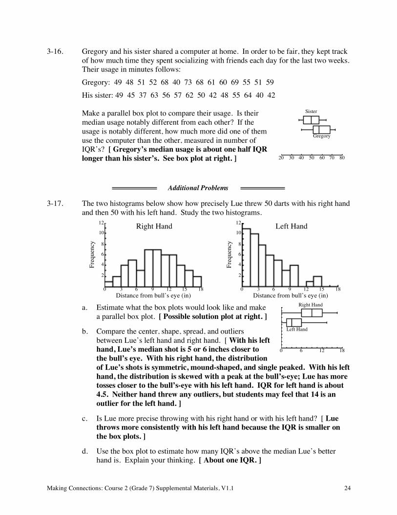
3-17. The two histograms below show how precisely Lue threw 50 darts with his right hand

and then 50 with his left hand. Study the two histograms.

a. Estimate what the box plots would look like and make a parallel box plot. [ Possible solution plot at right. ]

b. Compare the center, shape, spread, and outliers between Lue’s left hand and right hand. [ With his left hand, Lue’s median shot is 5 or 6 inches closer to the bull’s eye. With his right hand, the distribution of Lue’s shots is symmetric, mound-shaped, and single peaked. With his left hand, the distribution is skewed with a peak at the bull’s-eye; Lue has more tosses closer to the bull’s-eye with his left hand. IQR for left hand is about 4.5. Neither hand threw any outliers, but students may feel that 14 is an outlier for the left hand. ]

c. Is Lue more precise throwing with his right hand or with his left hand? [ Lue throws more consistently with his left hand because the IQR is smaller on the box plots. ]

d. Use the box plot to estimate how many IQR’s above the median Lue’s better hand is. Explain your thinking. [ About one IQR. ]

Additional Problems

20 30 50 40 60 70 80

Gregory

Sister

0 3 6 9 12 15 18

2

4

6

8

10

Distance from bull’s eye (in)

Freq

uenc

y

Right Hand 12

0 3 6 9 12 15 18

2

4

6

8

10

Distance from bull’s eye (in)

Freq

uenc

y Left Hand 12

0 6 12 18

Right Hand

Left Hand


3-18. Do honors students read more over the summer? Serena’s class asked 30 parents to estimate how many pages their child read over the summer. They collected the following data. Honors students: 10 30 230 130 110 240 150 260 60 230 100 20 50 160 90 pages

Regular students: 210 100 0 40 260 240 200 220 190 150 50 100 12 140 40 pages

a. Make parallel box plots and compare the center, shape, spread, and outliers. [ See plot at right. Center, shape, and spread are nearly identical for both groups. Median of regular students may be about 30 pages higher, but that difference is very small when compared to variability. Both distributions are symmetric. IQR is about 160-180 pages. Neither group has outliers. ]

b. Do honors students read more? How many IQR’s more (use the box plots to estimate)? [ We cannot conclude that honors students read more. The difference of 30 pages is less than 1/4 of an IQR. ]

0 50 100 150

Honors

Regular

200 250 300


Lesson 3.2.1 Is the survey fair? Representative Samples

Lesson Objective: Students will analyze methods of sampling and critique how well a sample represents a certain population.

Standards: CCSS: 7.SP 1. Understand that statistics can be used to gain information about a population by examining a sample of the population; generalizations about a population from a sample are valid only if the sample is representative of that population. [Understand that random sampling tends to produce representative samples and support valid inferences.]


Core Problems: Problems 3-19 through 3-23

Materials: None


Begin by asking a student volunteer to read the introduction and the focus questions. Then direct teams to work on problems 3-19 and 3-20. When they are done, bring the class together and conduct a whole class discussion about their answers. Students should understand the significance of who is interviewed in a survey. In problems 3-21 and 3-22, students continue to develop understanding about the appropriateness of a representative sample. Hold a class discussion about their responses before moving on. It is not important for students to be able to distinguish between different types of sampling techniques: they are not expected to know, for example, whether a given situation is a volunteer response sample or a cluster sample or a combination of both. The focus should be on whether a sample represents the population of interest well enough. In part (d) of problem 3-22 students are introduced to the notion that association does not imply causation. This topic will be covered in much more detail in the high school units, but it is important for students to be exposed to the notion early. They are bombarded with statistics on a daily basis.


Ask for student volunteers to recap what they have learned about representative samples. Use problem 3-23 as a culmination and summary of the lesson. The point of choosing a representative sample is to be able to make inferences about the whole population. Make sure students leave class today with this concept.




3.2.1 Is the survey fair? • • • • • • • • • • • • • • • • • • • • • • • • • • • • • • • • • • • • • • • • • • • • • • • • • • • • • • • • • • • • • • • • • • • • Representative Samples If you want to know what a bowl of soup tastes like, do you need to eat all of the soup in the bowl? Or can you get a good idea of the taste by trying a small sample? When conducting a survey, it is not usually possible to survey every person in the population you are interested in (all female teenage shoppers, students at your school, etc.). Instead, statisticians collect information about a sample (a portion) of the population. However, finding a representative sample (a sample that represents the whole population well) is not easy. 3-19. As social director on Class Council, Ramin would like to survey a few students about

their interests.

When Ramin analyzes the results from the survey, he wants to make claims about the interests of all of the students in school. If he were to survey only students in the Class Council, for example, it might be hard to make claims about what all students think. Students who are in Class Council may not have the same social interests as other students. Consider this idea as you think about the samples described below.

a. If Ramin wanted to generalize the opinions of all students at his school, would it make sense to go to the grocery store and survey the people there? Why or why not? [ No; That sample probably does not go to your school. ]

b. If he wanted to generalize the opinions of all students at his school, would it make sense to ask all of his friends at school? Why or why not? [ No; The students who are not his friends might have different sorts of opinions than his friends. ]

c. If he wanted to generalize the opinions of all students at his school, would it make sense to ask every third person who entered the cafeteria at lunch? Why or why not? [ No; While this is the best sample yet, it still does not include students who bring their own lunch. ]


3-20. There are a variety of ways to choose samples of the population you are studying. Every sample has features that make it more or less representative of the larger population. For example, if you want to represent all of the students at your school, but you survey all of the students at school 30 minutes after the last class has ended, you are likely to get a disproportionate number of students who play school sports, attend after school activities, or go to after school tutoring.

a. If you ask the opinion of the people around you, then you have used a convenience sample. If you took a convenience sample right now, what would be some features of the sample? Would you expect a convenience sample to represent the entire student population at your school? Why or why not? [ Students taking this math class; No: Reasons vary. ]

b. If you email or create an online questionnaire then you have used a voluntary response sample. What are some features of the people in a volunteer response sample? Could it represent well the sample of all of the students at school? [ They are people who regularly use a computer and who choose to respond. Probably not; Students may argue that people most likely to respond are people who feel most strongly about the issues being surveyed. ]

c. If you believe an existing group of people represent all of the students at your school well enough, this group is a cluster sample. What cluster of students might you survey at your school to represent all of the students at your school? Explain. Are there any reasons that this cluster might not be fully representative of all the students at your school? [ Some good cluster samples might be: Haphazard students at morning break because very few students leave campus for morning break; Students in a homeroom depending on how homerooms are selected; Students exiting a school-wide assembly; Students on registration day, depending on how registration is conducted. ]


3-21. From what population is each of these samples taken? Write down the actual population for each of these sampling techniques. [ See answers in bold in table below. ]

Method of Sampling Description of Actual Population

Call every hundredth name in the phone book.

People with phones who also have their numbers listed

Survey people who come to the “Vote Now” booth at the high school football game.

Athletic supporters who are interested enough in the topic to stop.

Ask every tenth student entering a high school football game.

A much better survey than above, but still limited only to athletic supporters.

Haphazardly survey students standing in the quad at morning break.

All students at the school.

Text response to an online “instant” poll. People who are using a computer and also a cell phone, who care strongly enough about the issue to respond.

Hand out surveys in the library before school.

“Studious” students.

Survey all students in Period 1 English classes.

Could represent all students at school, depending on how students are assigned to English class periods.


3-22. A study at the University of Iowa in 2008 concluded that children that play violent video games are more aggressive in real life. Children ages 9 to 12 were studied for how much they played violent video games; peers and teachers were asked how much these students hit, kicked, and got into fights with other students.

a. Can you legitimately conclude from this study that teenagers who play violent video games tend to be more aggressive? Why or why not? [ No; The sample did not include teenagers. ]

b. Can you legitimately conclude from this study that children ages 9 to 12 who play violent video games are more likely to commit violent crimes? Why or why not? [ No; crimes rates were not studied. ]

c. Can you legitimately conclude from this study that children ages 9 to 12 tend to hit and kick more in school? [ This study does indicate a relationship. ]

d. Can you legitimately conclude from this study that playing a lot of violent video games will cause 9 to 12-year-old students to become more violent at school? [ No; We can only say that there is a relationship between the two. We don’t know which is the cause and which is the effect. It might be that violent students are more attracted to violent video games. ]

3-23. Addie was helping children in a kindergarten class learn to read. She was curious

how old the typical child was when they entered kindergarten. It was not practical to look up the school records of all 100 kindergarteners. So on the first day of school, Addie took a sample: she asked the parent of the first fifteen students to be dropped off at the school how old (in months) their child was. Her data is listed below.

67 61 69 72 71 65 67 67 57 68 71 72 61 59 62 Make an inference (a statistical prediction) of the mean age of Kindergarteners at the school. [ 65.9 months ]


3-24. Suppose you were conducting a survey to try to determine what portion of voters in

your small town support a particular candidate for mayor. Consider each of the following methods for sampling the voting population of your town. State whether each is likely to produce a representative sample and explain your reasoning.

a. Ask every voter on your block. [ Not representative; neighborhoods in towns tend to have different characteristics from each other like wealth, ethnic makeup, proximity to services, traffic, etc. ]

b. Randomly pick one house from each block in the neighborhood and survey the homeowner. [ Fairly representative; but this will also survey non-voters. It would be better to survey only voters. ]

c. Survey each person at the pancake house after church on Sunday morning. [ Not representative; this samples the population of people who attend church and who favor the particular pancake house and have the time and money for a leisurely brunch. ]

d. Ask people who are leaving the twice-yearly town hall meeting. [ Possibly; It might be pretty representative because you will get active citizens who are also more likely to vote. But if a “hot topic” is on the agenda, you might get mostly those who are passionate about the one agenda item. ]

e. Visit every tenth person on the county’s voter registration list. [ This sample is just about the best you are going to get for a representative sample of voters. ]

3-25. Imagine that you and your team will be conducting a survey to see how many minutes

long lunch should be at your school. Students understand that the longer lunch is, the longer the school day is. Since you cannot ask every student, you will take a sample.

a. You ask every tenth student leaving the school-wide assembly to stop and think about how long they would like lunch to be. Do you think this sample is representative of the whole school? [ Yes, this is a good sample. ]

b. These are the answers of the first 20 students:

60 40 50 25 30 15 30 50 50 35 45 25 25 50 25 60 55 60 60 15 minutes

Make an inference (a statistical prediction) about the average length all students at your school think lunch should be. [ Mean 40.25 minutes, median is 42.5 minutes. Either mean or median is acceptable since the distribution is fairly symmetrical. ]

Additional Problems


Lesson 3.2.2 How close is my sample? Inference from Random Samples Lesson Objective: Students will use random sampling to draw inferences about a population.

They will generate multiple samples of the same size to gauge the variation in sample statistics.


Standards: CCSS: 7.SP 1. Understand that statistics can be used to gain information about a population by examining a sample of the population; generalizations about a population from a sample are valid only if the sample is representative of that population. Understand that random sampling tends to produce representative samples and support valid inferences. 7.SP 2. Use data from a random sample to draw inferences about a population with an unknown characteristic of interest. Generate multiple samples (or simulated samples) of the same size to gauge the variation in estimates or predictions.

Core Problems: Problems 3-26, 3-27, and 3-29

Materials: Envelopes, one per pair of students Scissors, one per pair of students Lesson 3.2.2 Resource Page, “A Whole Town of American Robins,” one per student


So that the cutting is not too disruptive later, start the class by having students prepare the envelopes. The envelopes can be used over and over, so only your first class needs to prepare them. Pass out the resource page, have students cut strips of rows or columns, and then cut them apart into little squares. Carefully place all 100 robins into the envelope. The envelope represents every robin in town; students will take a random sample of them to make an inference about the whole town’s population. Bring the class back together and have a student volunteer read the introduction and the beginning of problem 3-26 aloud. Then have students read the Math Notes box silently to themselves where prompted in part (a). Hold a whole-class discussion for part (b). Students can work in their teams on parts (c) through (e). Students will need a way to combine their data in part (a) of problem 3-27. Use the white board or an overhead projector. A whole-class discussion would be fruitful for parts (b) and (c). Part (c) very informally introduces students to the notion of a margin of error, although the term is never used. Using the IQR interval is adequate until more formal developments come in high school.


Problem 3-28 is additional reinforcement of this new concept of finding an interval that the population is probably within.

Closure: (10-15 minutes)

Allow plenty of time for problem 3-29 so that students can process their learning and write it down. Hold a class discussion of students’ ideas.


Problem 3-30 If students did not have enough time to process problem 3-29 individually in class, assign it for homework.


3.2.2 How close is my sample? • • • • • • • • • • • • • • • • • • • • • • • • • • • • • • • • • • • • • • • • • • • • • • • • • • • • • • • • • • • • • • • • • • • • • • • Inference from Random Samples In the previous lesson you studied techniques for sampling populations. If you wanted to know the average height of the trees in a forest you would not want to measure every tree in the forest. You would take a sample of the trees and measure them to give you a good prediction of the average height of all the trees. If you measured 10 trees and found the mean, you would get a number that describes those 10 trees, but how well does that number describe all of the trees in the entire forest? Let’s investigate similar situations. 3-26. The sighting of American robins in yards is considered a sign that spring has arrived.

You would like to know the average weight of an American robin in your town.

a. Of course you cannot weigh every robin in town, even if you could figure out how to catch them all. A sample seems like a good idea. Read the Math Notes box, “Random Samples,” that follows this lesson.

b. Think about how you can take a random sample from the population of robins in your envelope. What things would be important to do? Discuss this with your team. [ Sample responses include not looking in the envelope, choosing one at a time, stirring or shaking the envelope, replacing or not replacing the birds between samples. ]

c. Now take a random sample of ten robins from your envelope and record their weights. Each member of your team should do the same.

d. Calculate the mean of your sample. Do you think that your mean is representative of the population? What inferences can you make about the population from your sample? [ The sample is representative because it is random. Means will most likely be between 70g and 95g. ]

e. Compare your estimate of the population mean to your team’s means. Is your mean the true average weight for all American robins in town? Is your teammate’s the true average? How can you explain any differences between the means? [ Answers will vary, but might include that by chance one partner has particularly large or small birds in their sample. No sample can give the true mean, just like no measurement is exact from Lesson 3.1.1. ]


3-27. Your estimate of the mean will probably be a little larger or smaller than the true average weight of robins. Let’s explore how much larger or smaller your estimate might be than the true average.

a. Combine your estimate of the population mean with the rest of the class. Make a combination histogram and box plot of the data. Use a bin width of 5g on your histogram. [ See sample plot at right. ]

b. What causes variation in the sample means? That is, why are some of the sample means on your class graph so much larger or smaller than others? Why are so many of the sample means bunched up in the middle? [ Sample response: Some of the samples, just by chance, might have a lot of large birds or small birds in them, or, just by chance, there might be an outlier in the sample affecting the mean. But most of the samples will have mostly typical birds in them, so the means will bunch up in the middle. ]

c. Within what interval do you suppose the true mean weight of American Robins is? [ Typical answer: between 75 and 90g if using the histogram, or between 77g and 86g if using the first and third quartile on the box plot. ]

3-28. Cyrus plays volleyball in county-wide tournaments. He wondered what portion of

volleyball players prefer plain water over sports drinks during intense games.

a. At his next tournament, Cyrus selected 50 random players from all the teams to ask about their preference. 78% preferred plain water. What inference can Cyrus make about all the volleyball players in the county? [ 78% prefer plain water. Based on the previous problem, some students will indicate that the true percentage lies within an interval. ]

b. What additional information would Cyrus gain if it was practical to take many samples at many tournaments in the county? [ He would get an interval within which the true percentage probably lies. ]

c. If many samples could be taken, the distribution of percentages in each of the samples might look like this:

% preferring water: 84% 71% 73% 83% 80% 80% 79% 77% 81% 72% 81% 78%

Make a box plot of the samples. With this additional information, make a new statement about volleyball players and water. [ See box plot at right. The true percentage of volleyball payers in the county that prefer water over sports drinks is probably between 75% and 81%. ]

70 65 75 80 85 90 95 100

70 80 90


3-29. Make an entry in your notes and title it “Inferences From Random Samples.” Why would you want to take a sample instead of just testing the entire population? What is the best way to take a sample from a population? Why are random samples more representative of the population than other kinds of samples? What additional information would you have if you could take many samples from the same population? [ A random sample is helpful if testing the entire population is too time-consuming, costly, or impractical (like catching every robin). The best samples are random because they account for variables in the population you forgot about or did not even know about. By taking many samples, we would have an interval within which the true population characteristics probably fall. ]

3-30. Athena was working on her Girl Scouts silver award and was wondering what

percentage of people support Girl Scouts financially through cookie sales at the grocery store.

At the next cookie sale, Athena kept track of how many customers at the grocery store walked by the cookie table and how many stopped to purchase cookies. 32% of families stopped and purchased cookies at the table. Athena continued collecting data at several different grocery stores around town. Here are the percent of those who bought cookies at each store: 32% 29% 19% 31% 30% 24% 38% 33% 42% 25% 22% 27%

Make a box plot of the samples, then make a new statement about what proportion of people (in what interval) we can expect to but girl scout cookies at the grocery store. [ See box plot at right. The true percentage of grocery store shoppers that buy Girl Scout cookies is probably between 25% and 33%. ]

Additional Problems

10 25 50


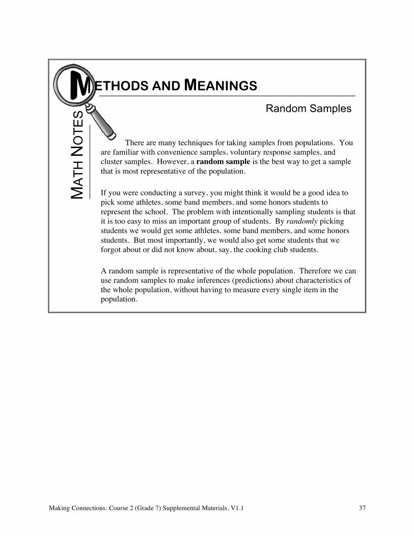
There are many techniques for taking samples from populations. You are familiar with convenience samples, voluntary response samples, and cluster samples. However, a random sample is the best way to get a sample that is most representative of the population.

If you were conducting a survey, you might think it would be a good idea to pick some athletes, some band members, and some honors students to represent the school. The problem with intentionally sampling students is that it is too easy to miss an important group of students. By randomly picking students we would get some athletes, some band members, and some honors students. But most importantly, we would also get some students that we forgot about or did not know about, say, the cooking club students.

A random sample is representative of the whole population. Therefore we can use random samples to make inferences (predictions) about characteristics of the whole population, without having to measure every single item in the population.

ETHODS AND MEANINGS M

ATH

NO

TES Random Samples


Lesson 3.2.2 Resource Page

A Whole Town of American Robins

66 102 115 60 59 122 106 119 113 63

83 89 74 54 86 87 104 103 74 103

86 103 87 86 114 79 95 93 91 99

27 73 86 83 41 59 49 104 97 46

40 98 67 82 70 74 117 78 108 103

42 57 87 81 61 72 80 67 53 103

98 91 63 103 114 60 79 69 115 66

62 72 78 63 75 87 82 73 82 71

78 95 89 73 76 92 64 84 76 95

97 81 76 79 71 96 108 67 89 42


Lesson 2.2.2 What if it is too complicated? Computer Simulations of Probabilities Lesson Objective: Students will use a computer simulation to find experimental

probabilities of complex compound probabilities.

Standards: CCSS: 7-SP8c. Design and use a simulation to generate frequencies for compound events. NCTM: Use proportionality and a basic understanding of probability to make and test conjectures about the results of experiments and simulations.


Core Problems: Problems 2-75 to 2-76

Materials: Random Number Generator, one per pair or team (see Technology section in the prologue to Unit 2).

Technology Notes: Study teams will need a Random Number Generator that produces the numbers from 1 through 20. See the Technology section in the prologue to Unit 2. If you are using graphing calculators, remember to seed the random number generator as indicated in the Technology section.


Direct teams to read the focus questions in the lesson introduction, and then to begin work on problem 2-75. It may be necessary to explain to the class what a random number generator is, but do not distribute the technology yet. Students should complete parts (a) and (b) before beginning to play the game in part (c). To generate the ten random numbers needed for problem 2-75, enter “randInt(1,20,10)” on the TI83+/TI-84+ calculator. Figuring out the theoretical probability for problem 2-76 is challenging, even for college students. This type of problem, then, leads itself nicely to being estimated with a computer simulation. Professional statisticians might even check their answers to a theoretical calculation with a simulation like this. To simulate the five action figures purchased over the course of the summer in problem 2-76, enter “randInt(1,3,5)” on the TI83+/TI-84+ calculator. To simulate a family of three children in problem 2-77, enter “randInt(0,1,3)” on the TI83+/TI-84+ calculator. The “1” can stand for a girl, and the “0” for a boy. The theoretical probability for compound probabilities such as this one will be developed starting in the next lesson. Do not attempt to explain the theoretical probability to students at this stage.


To simulate rolling two dice in problem 2-78, enter “randInt(1,6,2)” on the TI83+/TI-84+ calculator.


Part (b) of problem 2-78 can be used as a closure discussion. Again, do not attempt to explain the theoretical probability at this juncture. Development of the theory will begin in the next lesson.




2.2.2 What if it is too complicated? • • • • • • • • • • • • • • • • • • • • • • • • • • • • • • • • • • • • • • • • • • • • • • • • • • • • • • • • • • • • • • • • • Computer Simulations of Probability If you toss a coin ten times, what is the probability of having a run of three or more “heads” in a row? If an airline “overbooks” a certain flight, what is the chance more passengers show up than the airplane has seats for? When 67 people get cancer in the 250 homes in a small town, could that be due to chance alone, or is polluted well water a more likely explanation of the cluster of cancer cases? When the mathematics becomes too complicated to figure out the theoretical probability of certain events, statisticians often use computer simulations instead. All simulations require the use of random numbers. Random numbers have no pattern; they cannot be predicted in any way. Knowing a random number in no way allows you to predict the next random number. An example of a random number generator is a standard number cube, which will randomly generate a number from 1 to 6 when you roll it. Complex simulations like modeling the weather, traffic patterns, cancer radiation therapy, or stock market swings require tens of billions of random numbers. For those simulations a large computer running for hours or even days is needed, but many simple simulations can be done with classroom technology. 2-75. RANDOM NUMBER GENERATOR

Imagine a random number generator that produces numbers from 1 to 20. In each game below, if the stated outcome happens, Player X wins. If it does not, then Player Y wins.

Game 1: A prime number = Player X wins Game 2: An even number = Player X wins Game 3: A number not divisible by three = Player X wins

a. In each case, what is the theoretical probability that Player X wins? That Player Y wins? Decide whether each game above is fair. [ a: Game 1: P(prime) = 8

20 , P(not prime) = 12

20 , not fair; Game 2: P(even) = 1020 = 1

2 , P(odd) = 1020 = 1

2 , fair; Game 3: P(not div by 3) = 14

20 , P(div by 3) = 620 , not fair. ]

b. In which of the three games is Player X most likely to win? Why? [ Game 3 ]

c. In Game 1, the prime number game, if you play 40 times, how many times would you expect Player X to win? What if you played 50 times? [ About 16 times; About 20 times. ]

Problem continues on next page. →


2-75. Problem continued from previous page.

d. Obtain a random number generator from your teacher and set it up to generate integers from 1 to 20. Play the prime number game (Game 1) 10 times with a partner. Start by deciding who will be Player X and who will be Player Y. Record who wins each time you play.

e. How did the experimental and theoretical probabilities of Player X winning from part (a) and part (d) compare? [ Answers vary based on experimental results. ]

2-76. Janelle is going to baby-sit her nephew all day long five times this summer. She had

the great idea that one way to entertain him is to walk to McBurger’s for a Kids Meal for lunch each time. The Kids Meal comes packed randomly with one of three possible action figures. Janelle would like to know the probability that they get all three figures in five trips.

a. Call the action figures #1, #2, and #3. Your teacher will show you how to use a random number generator to simulate five trips to McBurger’s. Did you get all three action figures?

b. Simulate another five trips to McBurger’s. Did you get all five action figures this time? Do the simulation at least 20 times, keeping track of how many times you got all five action figures, and how many times you did not.

c. Use your results to estimate the probability of getting all five action figures this summer. Should Janelle be worried? [ Theoretical probability is about 0.62. ]

d. How could Janelle get an even more accurate estimation of the probability? [ Run more simulations, or combine results with other teams in the class. ]

2-77. Janelle’s aunt and uncle had three children. Two of them were girls. Since girls and

boys are equally likely, Janelle thought that the chance of having two or more girls must be 50%. Janelle’s brother thought the chance of having so many girls had to be less than 50%.

a. What do you think? Make a conjecture about the probability of having two or three girls in a family of three siblings.

b. Do a computer simulation to estimate the probability of having two or three girls in a family of three siblings. Your teacher will show you how to simulate a family of three siblings. [ Theoretical probability is 0.5. ]


2-78. Sophia and her brother are trying to create a fair game in which you roll two dice. They cannot agree on the probability of both numbers being even, so they decide to design a simulation.

a. Make a conjecture. What is the probability both dice are even? [ Students may answer 50% since odd and even are equally likely. ]

b. Design a simulation with a random number generator. How many random numbers do you need? In what interval should the numbers be? How many times will you do the simulation. [ Two random numbers in the interval from 1 to 6. The more trials, time allowing, the closer the simulated probability will be to the theoretical probability. ]

c. Your teacher will help you set up the simulation that you designed. Do you want to revise your conjecture from part (a)? [ Theoretical probability is 0.25. ]

2-79. A BETTER CHANCE OF WINNING Each of the problems below describes two different games you can play with a

random number generator. In each case, you will win if the random number generator gives you the indicated kind of number. Find the theoretical probability that you win each game below. Decide and justify whether Game I or Game II in each part gives you a better chance of winning. [ a: 820 > 4

20 , Game I; b: 420 = 840 ,

equal chance; c: 540 < 425 or12.5%< 16% , Game II. ]

Game I Game II

a. Picking a prime number from the integers between 1 and 20

Picking a prime number from the integers between 21 and 40

b. Picking a multiple of 5 from the integers between 1 and 20

Picking a multiple of 5 from the integers between 1 and 40

c. Picking a multiple of 7 from the integers between 1 and 40

Picking a multiple of 6 from the integers between 1 and 25

Additional Problems


2-80. If you used a random number generator for the numbers from 1 through 20 to play a game, what is the theoretical probability of getting each of these outcomes? [ a: 820 , b: 1, c: 920 , d: Answers will vary. ]

a. A multiple of three or a multiple of 7, P(multiple of 3 or multiple of 7)

b. P(even or odd)

c. P(prime or 1)

d. How did you find the probabilities of these events? Be ready to share your ideas with the class.

2-81. Nicole has a random number generator that will produce the numbers from 1 through

50 when she pushes a button. If she pushes the button, what is: [ a: 550 , b: 1, c: 3850 , d: 950 ]

a. P(multiple of 10) ? b. P(not 100) ?

c. P(not a multiple of 4)? d. P(one-digit number) ?

CCSS Grade 7 TV V1.1 - CPM Educational Program

Documents

Transcript of CCSS Grade 7 TV V1.1 - CPM Educational Program