CBMS Lecture Series Recent Advances in the Numerical...
160
CBMS Lecture Series Recent Advances in the Numerical Approximation of Stochastic Partial Differential Equations or more accurately Taylor Approximations of Stochastic Partial Differential Equations A. Jentzen Department of Mathematics Universit¨atBielefeld Bielefeld, Germany Email: [email protected] P.E. Kloeden Institut f¨ ur Mathematik GoetheUniversit¨at Frankfurt am Main, Germany Email: [email protected] 1
Transcript of CBMS Lecture Series Recent Advances in the Numerical...
CBMS Lecture Series
Recent Advances in
the Numerical Approximation
of Stochastic Partial Differential Equations
or more accurately
Taylor Approximations
of Stochastic Partial Differential Equations
A. Jentzen
Department of Mathematics
Universitat Bielefeld
Bielefeld, Germany
Email: [email protected]
P.E. Kloeden
Institut fur Mathematik
Goethe Universitat
Frankfurt am Main, Germany
Email: [email protected]
1
10 Lectures on Taylor Expansions!!
Taylor expansions are a very basic tool in numerical analysis and other areas
of mathematics that require approximations.
They enable the derivation of one–step numerical schemes for differential equa-
tions of arbitrary high order.
1. Ordinary Differential Equations
2. Random Ordinary Differential Equations
3. Stochastic Ordinary Differential Equations
4. Stochastic Ordinary Differential Equations:
Nonstandard Assumptions
5. Stochastic Partial Differential Equations:
Introduction
6. Stochastic Partial Differential Equations:
Numerical Methods
7. & 8. Stochastic Partial Differential Equations:
Additive Noise I & II
9. & 10. Stochastic Partial Differential Equations:
Multiplicative Noise I & II
2
Lecture 1: Ordinary Differential Equations
The Taylor expansion of a p + 1 times continuously differentiable function x :
R → R is given by
x(t) = x(t0) + x′(t0) h + . . . +1
p!x(p)(t0) hp +
1
(p + 1)!x(p+1)(θ) hp+1 (1)
with the remainder term evaluated at some intermediate value θ ∈ [t0, t], which is
usually unknown. Here h = t − t0.
1 Taylor Expansions for ODEs
Let x(t) = x(t, t0, x0) be the solution of a scalar ODE
dx
dt= f(t, x), (2)
with the initial value x(t0) = x0 and define the differential operator L by
Lg(t, x) :=∂g
∂t(t, x) + f(t, x)
∂g
∂x(t, x),
i.e., Lg(t, x(t)) is the total derivative of g(t, x(t)) with respect to a solution x(t) of
the ODE (2), since
d
dtg(t, x(t)) =
∂g
∂t(t, x(t)) +
∂g
∂x(t, x(t)) x′(t) = Lg(t, x(t))
by the chain rule.
1
In particular, for any such solution
x′(t) = f(t, x(t))
x′′(t) =d
dtx′(t) =
d
dtf(t, x(t)) = Lf(t, x(t))
x′′′(t) =d
dtx′′(t) =
d
dtLf(t, x(t)) = L2f(t, x(t)) ,
and, in general,
x(j)(t) = Lj−1f(t, x(t)), j = 1, 2, . . . ,
provided f is smooth enough.
For notational convenience, define L0f(t, x) ≡ f(t, x).
If f is p times continuously differentiable, then the solution x(t) of the ODE
(2) is p+1 times continuously differentiable and has a Taylor expansion (1), which
can be rewritten as
x(t) = x(t0) +
p∑
j=1
1
j!Lj−1f(t0, x(t0)) (t − t0)
j
+1
(p + 1)!Lpf(θ, x(θ)) (t − t0)
p+1.
On a subinterval [tn, tn+1] with h = tn+1 − tn > 0, the Taylor expansion is
x(tn+1) = x(tn) +
p∑
j=1
1
j!Lj−1f(tn, x(tn)) hj +
1
(p + 1)!Lpf(θn, x(θn)) hp+1 (3)
for some θn ∈ [tn, tn+1], which is usually unknown.
2
Nevertheless, the error term can be estimated and is of order 0(hp+1), since
hp+1
(p + 1)!|Lpf(θn, x(θn; tn, xn))| ≤
hp+1
(p + 1)!max
t0≤t≤T
x∈D
|Lpf(t, x)| ≤ Cp,T,D hp+1,
where D is some sufficiently large compact subset of R containing the solution over
a bounded time interval [t0, T ] which contains the subintervals under consideration.
The maximum can be used here since Lpf is continuous on [t0, T ] × D.
Note that Lpf contains the partial derivatives of f of up to order p.
2 Taylor schemes for ODEs
The Taylor scheme of order p for the ODE (2),
xn+1 = xn +
p∑
j=1
hj
j!Lj−1f(tn, xn), (4)
is obtained by discarding the remainder term in the Taylor expansion (3) and re-
placing x(tn) by xn.
The Taylor scheme (4) is an example of one–step explicit scheme which has the
general form
xn+1 = xn + hF (h, tn, xn) (5)
with an increment function F defined by
F (h, t, x) :=
p∑
j=1
1
j!Lj−1f(t, x) hj−1.
3

A one–step explicit scheme is said to have order p if its global discretisation error
Gn(h) := |x(tn, t0, x0) − xn| , n = 0, 1, . . . , Nh :=T − t0
h,
converges with order p, i.e., if
max0≤n≤Nh
Gn(h) ≤ Cp,T,D hp.
A basic result in numerical analyis says that a one–step explicit scheme converges
with order p if its local discretisation error converges with order p + 1. This is
defined by
Ln+1(h) := |x(tn+1) − x(tn) − hF (h, tn, x(tn))| ,
i.e., the error on each subinterval taking one interation of the scheme starting at
the exact value of the solution x(tn) at time tn.
• Thus, the Taylor scheme of order p is indeed a pth order scheme.
The simplest nontrivial Taylor scheme is the Euler scheme
xn+1 = xn + hf(tn, xn),
which has order p = 1.
4
The higher coefficients Lj−1f(t, x) of a Taylor scheme of order p > 1 are, however,
very complicated.
For example,
L2f = L[Lf ] =∂
∂t[Lf ] + f
∂
∂x[Lf ]
=∂
∂t
∂f
∂t+ f
∂f
∂x
+ f∂
∂x
∂f
∂t+ f
∂f
∂x
=∂2f
∂t2+
∂f
∂t
∂f
∂x+ f
∂2f
∂t∂x+ f
∂2f
∂x∂t+ f
(
∂f
∂x
)2
+ f 2 ∂2f
∂x2
and this is just the scalar case!!
Taylor schemes are thus rarely used in practice, but they are very useful for theo-
retical purposes,
e.g., for determining by comparison the local discretization order of other numerical
schemes derived by heuristic means such as the Heun scheme
xn+1 = xn +1
2h [f(tn, xn) + f(tn+1, xn + hf(tn, xn))] ,
which is a Runge-Kutta scheme of order 2.
Symbolic manipulators now greatly facilitate the use of Taylor schemes. Indeed,
B. Coomes, H. Kocak and K. Palmer, Rigorous computational shadowing
of orbits of ordinary differential equations, Numerische Mathematik 69 (1995),
no. 4, 401–421.
applied a Taylor scheme of order 31 to the 3-dimensional Lorenz equations.
5

3 Integral representation of Taylor expansion
Taylor expansions of a solution x(t) = x(t, t0, x0) of an ODE (2) also have an
integral derivation and representation.
These are based on the integral equation representation of the initial value problem
of the ODE,
x(t) = x0 +
∫ t
t0
f(s, x(s)) ds. (6)
By the Fundamental Theorem of Calculus, the integral form of the total derivative
is
g(t, x(t)) = g(t0, x0) +
∫ t
t0
Lg(s, x(s)) ds. (7)
Note that (7) reduces to the integral equation (6) with g(t, x) = x, since Lg = f
in this case.
Applying (7) with g = f over the interval [t0, s] to the integrand of the integral
equation (6) gives
x(t) = x0 +
∫ t
t0
[
f(t0, x0) + +
∫ s
t0
Lf(τ, x(τ)) dτ
]
ds
= x0 + f(t0, x0)
∫ t
t0
ds +
∫ t
t0
∫ s
t0
Lf(τ, x(τ)) dτ ds,
which is the first order Taylor expansion.
6
Then, applying (7) with g = Lf over the interval [t0, τ ] to the integrand in the
double integral remainder term leads to
x(t) = x0 + f(t0, x0)
∫ t
t0
ds + Lf(t0, x0)
∫ t
t0
∫ s
t0
dτ ds
+
∫ t
t0
∫ s
t0
∫ τ
t0
L2f(ρ, x(ρ)) dρ dτ ds.
In this way one obtains the Taylor expansion in integral form
x(t) = x(t0) +
p∑
j=1
Lj−1f(t0, x0)
∫ t
t0
∫ s1
t0
· · ·
∫ sj−1
t0
dsj · · · ds1
+
∫ t
t0
∫ s1
t0
. . .
∫ sj
t0
Lpf(sj+1, x(sj+1)) dsj+1 · · · ds1,
where for j = 1 there is just a single integral over t0 ≤ s1 ≤ t.
This is equivalent to the differential form of the Taylor expansion (3) by the Inte-
mediate Value Theorem for Integrals and the fact that
∫ t
t0
∫ s1
t0
· · ·
∫ sj−1
t0
dsj · · · ds1 =1
j!(t − t0)
j, j = 1, 2, . . . .
7
Lecture 2: Random Ordinary Differential
Equations
Random ordinary differential equations (RODEs) are pathwise ODEs that
contain a stochastic process in their vector field functions.
Typically, the driving stochastic process has at most Holder continuous
sample paths, so the sample paths of the solutions are certainly continuously
differentiable. However, the derivatives of the solution sample paths are at
most Holder continuous in time.
Thus, after insertion of the driving stochastic process, the resulting vector
field is at most Holder continuous in time, no matter how smooth the vector
field is in its original variables.
Consequently, although classical numerical schemes for ODEs can be used
pathwise for RODEs, they rarely attain their traditional order and new
forms of higher order schemes are required.
1
Let
• (Ω,F , P) be a complete probability space
• (ζt)t∈[0,T ] be an Rm-valued stochastic process with continuous sample paths
• f : Rm × R
d → Rd be a continuous function.
A random ordinary differential equation in Rd,
dx
dt= f(ζt(ω), x), x ∈ R
d, (1)
is a nonautonomous ordinary differential equation (ODE)
dx
dt= Fω(t, x) := f(ζt(ω), x) (2)
for almost every ω ∈ Ω.
A simple example of a scalar RODE is
dx
dt= −x + sin Wt(ω),
where Wt is a scalar Wiener process.
Here f(z, x) = −x + sin z and d = m = 1.
• Other kinds of noise such as fractional Brownian motion can also be used.
2
It will be assumed that f is infinitely often continuously differentiable in its vari-
ables, although k-times continuously differentiable with k sufficiently large would
suffice.
Then f is locally Lipschitz in x and the initial value problem
d
dtxt(ω) = f(ζt(ω), xt(ω)), x0(ω) = X0(ω), (3)
where the initial value X0 is a Rd-valued random variable, has a unique pathwise
solution xt(ω) for every ω ∈ Ω, which will be assumed to exist on the finite time
interval [0, T ] under consideration.
• Sufficient conditions guaranteeing the existence and uniqueness of solutions of
(3) are similar to those for ODEs.
The solution of the RODE (3) is a stochastic process (xt)t∈[0,T ], which is nonan-
ticipative if the driving process ζt is nonanticipative and independent of the initial
condition X0.
Important: The sample paths t → xt(ω) of a RODE are continuously differen-
tiable. They need not be further differentiable, since the vector field Fω(t, x) of the
nonautonomous ODE (2) is usually only continuous, but not differentiable in t, no
matter how smooth the function f is in its variables.
3
1 Equivalence of RODEs and SODEs
RODEs with Wiener processes can be rewritten as SODEs, so results for one can
be applied to the other. For example, the scalar RODE
dx
dt= −x + sin Wt(ω)
can be rewritten as the 2-dimensional SODE
d
Xt
Yt
=
−Xt + sin Yt
0
dt +
0
1
dWt.
On the other hand, any finite dimensional SODE can be transformed to a RODE.
This is the famous Doss–Sussmann result.
It is easily illustrated for a scalar SODE with additive noise: the SODE
dXt = f(Xt) dt + dWt
is equivalent to the RODE
dz
dt= f(z + Ot) + Ot, (4)
where z(t) := Xt −Ot and Ot is the Ornstein–Uhlenbeck stochastic stationary
process satisfying the linear SDE
dOt = −Ot dt + dWt.
4
To see this, subtract integral versions of both SODEs and substitute to obtain
z(t) = z(0) +
∫ t
0
[f(z(s) + Os) + Os] ds.
It follows by continuity and the Fundamental Theorem of Calculus that z is path-
wise differentiable. In particular, deterministic calculus can be used pathwise for
SODEs via RODEs.
This greatly facilitates the investigation of dynamical behaviour and other qualita-
tive properties of SODEs. For example, suppose that f in the RODE (4) satisfies
a one–sided dissipative Lipschitz condition (L > 0),
〈x − y, f(x) − f(y)〉 ≤ −L|x − y|2, ∀x, y ∈ R.
Then, for any two solutions z1(t) and z2(t) of the RODE (4),
d
dt|z1(t) − z2(t)|
2 = 2
⟨
z1(t) − z2(t),dz1
dt−
dz2
dt
⟩
= 2 〈z1(t) − z2(t), f(z1(t) + Ot) − f(z2(t) + Ot)〉
≤ −L |z1(t) − z2(t)|2,
from which it follows that
|z1(t) − z2(t)|2 ≤ e−2Lt|z1(0) − z2(0)|2 → 0 as t → ∞ (pathwise).
By the theory of random dynamical systems, there thus exists a pathwise asymp-
totically stable stochastic stationary solution. Transforming back to the SODE,
one concludes that the SODE also has a pathwise asymptotically stable stochastic
stationary solution.
5
2 Simple Numerical schemes for RODEs
The rules of deterministic calculus apply pathwise to RODEs, but the vector field
function in Fω(t, x) in (2) is not smooth in t.
It is at most Holder continuous in time like the driving stochastic process ζt and thus
lacks the smoothness needed to justify the Taylor expansions and the error analysis
of traditional numerical methods for ODEs.
Such methods can be used, but will attain at best a low convergence order, so new
higher order numerical schemes must be derived for RODEs.
For example, let t → ζt(ω) be pathwise Holder continuous with Holder exponent
12.
The Euler scheme
Yn+1(ω) = (1 − ∆n) Yn(ω) + ζtn(ω) ∆n
for the RODE
dx
dt= −x + ζt(ω),
attains the pathwise order 12.
One can do better by using the pathwise averaged Euler scheme
Yn+1(ω) = (1 − ∆n) Yn(ω) +
∫ tn+1
tn
ζt(ω) dt,
which was proposed in
L. Grune and P.E. Kloeden, Pathwise approximation of random ordinary dif-
ferential equations, BIT 41 (2001), 710–721.
6

It attains the pathwise order 1 provided the integral is approximated with Riemann
sums
∫ tn+1
tn
ζt(ω) dt ≈
J∆n∑
j=1
ζtn+jδ(ω) δ
with the step size δ satisfying δ1/2 ≈ ∆n and δ · J∆n= ∆n.
In fact, this was proved for RODEs with an affine structure, i.e., of the form
dx
dt= g(x) + H(x)ζt,
where g : Rd → R
d and H : Rd → R
d × Rm and ζt is an m-dimensional process.
The explicit averaged Euler scheme here is
Yn+1 = Yn + [g (Yn) + H (Yn) In] ∆n,
where
In(ω) :=1
∆n
∫ tn+1
tn
ζs(ω) ds.
For the general RODE (1) this suggests that one could pathwise average the vector
field, i.e.,
1
∆n
∫ tn+1
tn
f (ζs(ω), Yn(ω)) ds,
which is computationally expensive even for low dimensional systems.
An better alternative is to use the averaged noise within the vector field, which
gives the general averaged Euler scheme
Yn+1 = Yn + f (In, Yn) ∆n.
7
3 Taylor–like expansions for RODEs
Taylor–like expansions were used to derive systematically higher order numerical
schemes for RODEs in
P.E. Kloeden and A. Jentzen, Pathwise convergent higher order numerical
schemes for random ordinary differential equations, Proc. Roy. Soc. London, Series
A 463 (2007), 2929–2944.
A. Jentzen and P. E. Kloeden, Pathwise Taylor schemes for random ordinary
differential equations, BIT 49 (1) (2009), 113–140.
even though the solutions of RODES are at most continuously differentiable.
To emphasize the role of the sample paths of the driving stochastic process ζt, a
canonical sample space Ω = C(R+, Rm) of continuous functions from ω : R+ → R
m
will be used, so ζt(ω) = ω(t) for t ∈ R+.
The RODE (1) will henceforth be written
dx
dt= f(ω(t), x),
Since f is assumed to be infinitely often continuously differentiable in its variables,
the initial value problem (3) has a unique solution, which will be assumed to exist
on a finite time interval [t0, T ] under consideration.
By the continuity of the solution x(t) = x(t; t0, x0, ω) on [t0, T ], there exists an R
= R(ω, T ) > 0 such that
|x(t)| ≤ R(ω, T ) for all t ∈ [t0, T ].
8
Holder continuity of the noise
It will be assumed that the sample paths of ζt are locally Holder continuous with
the same Holder exponent,
i.e., there is a γ ∈ (0, 1] such that for P almost all ω ∈ Ω and each T > 0 there
exists a Cω,T > 0 such that
|ω(t) − ω(s)| ≤ Cω,T · |t − s|γ for all 0 ≤ s, t ≤ T. (5)
For such sample paths ω define
‖ω‖∞ := supt∈[t0,T ]
|ω(t)|, ‖ω‖γ := ‖ω‖∞ + sups6=t∈[t0,T ]
|t−s|≤1
|ω(t) − ω(s)|
|t − s|γ,
so
|ω(t) − ω(s)| ≤ ‖ω‖γ · |t − s|γ for all s, t ∈ [t0, T ].
Let θ be the supremum of all γ with this property.
• Two cases will be distinguished: Case A in which (5) also holds for θ itself
and Case B when it does not.
The Wiener process with θ = 12
is an example of Case B.
9
4 Multi–index notation
Let N0 denote the nonnegative integers. For a multi–index α = (α1, α2) ∈ N20 define
|α| := α1 + α2 , α! := α1! α2!
For a given γ ∈ (0, 1] define the weighted magnitude of a multi-index α by
|α|γ := γ α1 + α2
For each K ∈ R+ with K ≥ |α|γ define |α|Kγ := K − |α|γ.
For f ∈ C∞(R × U, R ) denote
fα := ∂αf := (∂1)α1(∂2)
α2f
with ∂(0,0)f = f and (0, 0)! = 1.
Let R(ω, T ) > 0 be an upper bound on the solution of the initial value problem
(3) corresponding to the sample path ω on a fixed interval [t0, T ] and define
‖f‖k := max|α|≤k
sup|y|≤‖ω‖∞|z|≤R
|fα(y, z)|.
For brevity, write ‖f‖ := ‖f‖0.
Note that the solution of the initial value problem (3) is Lipschitz continuous with
|x(t)−x(s)| ≤ ‖f‖ |t− s| for all s, t ∈ [t0, T ].
10
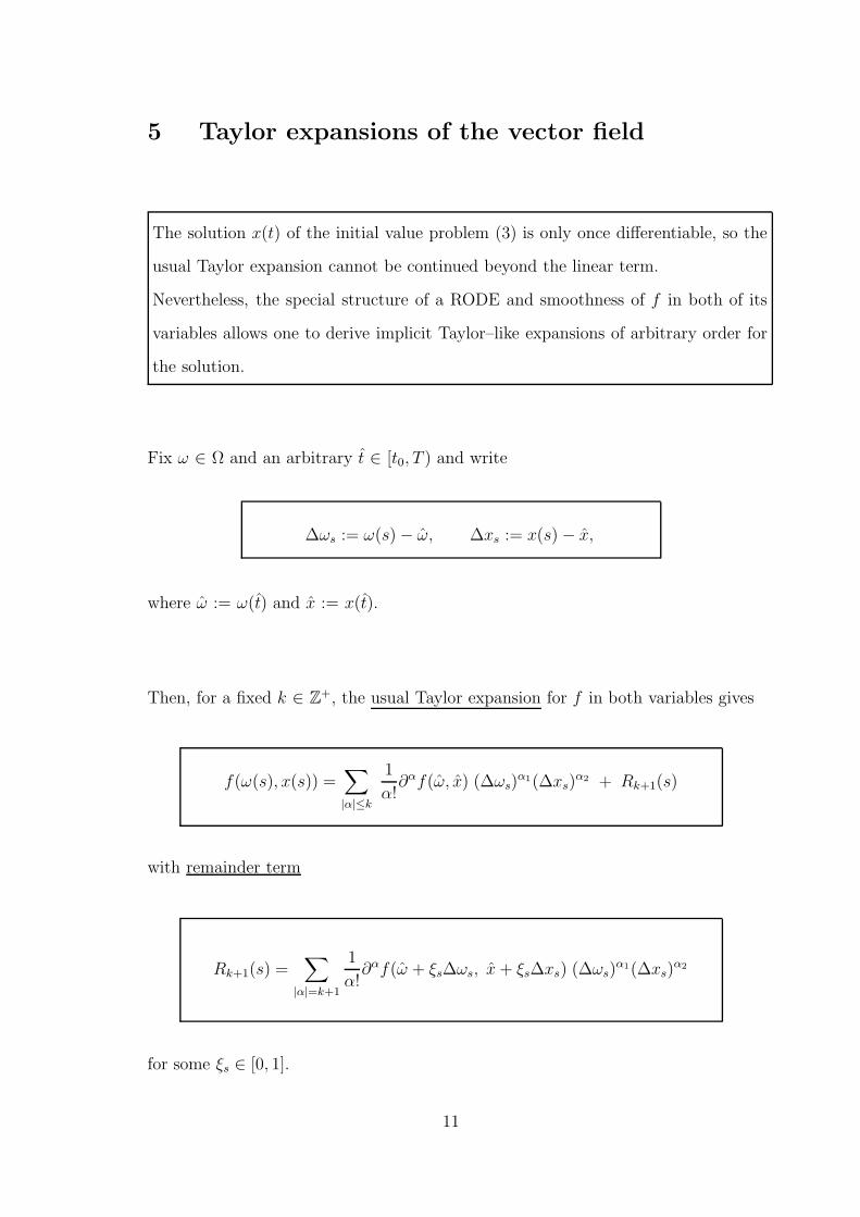
5 Taylor expansions of the vector field
The solution x(t) of the initial value problem (3) is only once differentiable, so the
usual Taylor expansion cannot be continued beyond the linear term.
Nevertheless, the special structure of a RODE and smoothness of f in both of its
variables allows one to derive implicit Taylor–like expansions of arbitrary order for
the solution.
Fix ω ∈ Ω and an arbitrary t ∈ [t0, T ) and write
∆ωs := ω(s) − ω, ∆xs := x(s) − x,
where ω := ω(t) and x := x(t).
Then, for a fixed k ∈ Z+, the usual Taylor expansion for f in both variables gives
f(ω(s), x(s)) =∑
|α|≤k
1
α!∂αf(ω, x) (∆ωs)
α1(∆xs)α2 + Rk+1(s)
with remainder term
Rk+1(s) =∑
|α|=k+1
1
α!∂αf(ω + ξs∆ωs, x + ξs∆xs) (∆ωs)
α1(∆xs)α2
for some ξs ∈ [0, 1].
11
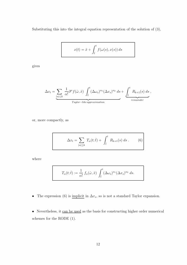
Substituting this into the integral equation representation of the solution of (3),
x(t) = x +
∫ t
t
f(ω(s), x(s)) ds
gives
∆xt =∑
|α|≤k
1
α!∂αf(ω, x)
∫ t
t
(∆ωs)α1(∆xs)
α2 ds
︸ ︷︷ ︸
Taylor−like approximation
+
∫ t
t
Rk+1(s) ds
︸ ︷︷ ︸
remainder
,
or, more compactly, as
∆xt =∑
|α|≤k
Tα(t; t) +
∫ t
t
Rk+1(s) ds . (6)
where
Tα(t; t) :=1
α!fα(ω, x)
∫ t
t
(∆ωs)α1(∆xs)
α2 ds.
• The expression (6) is implicit in ∆xs, so is not a standard Taylor expansion.
• Nevertheless, it can be used as the basis for constructing higher order numerical
schemes for the RODE (1).
12
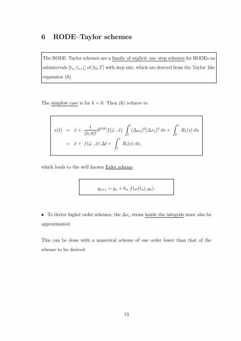
6 RODE–Taylor schemes
The RODE–Taylor schemes are a family of explicit one–step schemes for RODEs on
subintervals [tn, tn+1] of [t0, T ] with step size, which are derived from the Taylor–like
expansion (6).
The simplest case is for k = 0. Then (6) reduces to
x(t) = x +1
(0, 0)!∂(0,0)f(ω , x)
∫ t
t
(∆ωs)0(∆xs)
0 ds +
∫ t
t
R1(s) ds
= x + f(ω , x) ∆t +
∫ t
t
R1(s) ds,
which leads to the well known Euler scheme
yn+1 = yn + hn f(ω(tn), yn).
• To derive higher order schemes, the ∆xs terms inside the integrals must also be
approximated.
This can be done with a numerical scheme of one order lower than that of the
scheme to be derived.
13
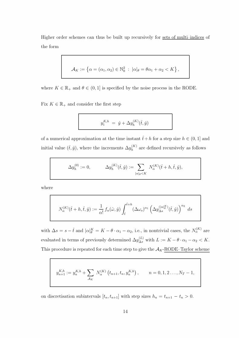
Higher order schemes can thus be built up recursively for sets of multi–indices of
the form
AK :=
α = (α1, α2) ∈ N20 : |α|θ = θα1 + α2 < K
,
where K ∈ R+ and θ ∈ (0, 1] is specified by the noise process in the RODE.
Fix K ∈ R+ and consider the first step
yK,h1 = y + ∆y
(K)h (t, y)
of a numerical approximation at the time instant t+h for a step size h ∈ (0, 1] and
initial value (t, y), where the increments ∆y(K)h are defined recursively as follows
∆y(0)h := 0, ∆y
(K)h (t, y) :=
∑
|α|θ<K
N (K)α (t + h, t, y),
where
N (K)α (t + h, t, y) :=
1
α!fα(ω, y)
∫ t+h
t
(∆ωs)α1
(
∆y(|α|K
θ)
∆s (t, y))α2
ds
with ∆s = s− t and |α|Kθ = K − θ · α1 − α2, i.e., in nontrivial cases, the N(K)α are
evaluated in terms of previously determined ∆y(L)∆s with L := K − θ ·α1 −α2 < K.
This procedure is repeated for each time step to give the AK-RODE–Taylor scheme
yK,hn+1 := yK,h
n +∑
AK
N (K)α
(
tn+1, tn, yK,hn
)
, n = 0, 1, 2 . . . , NT − 1,
on discretisation subintervals [tn, tn+1] with step sizes hn = tn+1 − tn > 0.
14
7 Discretisation error
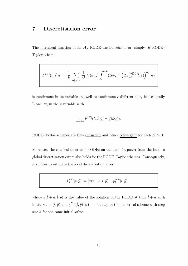
The increment function of an AK-RODE–Taylor scheme or, simply, K-RODE–
Taylor scheme
F (K)(h, t, y) :=1
h
∑
|α|θ<K
1
α!fα(ω, y)
∫ t+h
t
(∆ωs)α1
(
∆y(|α|K
θ)
∆s (t, y))α2
ds
is continuous in its variables as well as continuously differentiable, hence locally
Lipschitz, in the y variable with
limh→0+
F (K)(h, t, y) = f(ω, y).
RODE–Taylor schemes are thus consistent and hence convergent for each K > 0.
Moreover, the classical theorem for ODEs on the loss of a power from the local to
global discretisation errors also holds for the RODE–Taylor schemes. Consequently,
it suffices to estimate the local discretisation error
L(K)h (t, y) :=
∣
∣
∣x(t + h, t, y) − y
K,h1 (t, y)
∣
∣
∣,
where x(t + h, t, y) is the value of the solution of the RODE at time t + h with
initial value (t, y) and yK,h1 (t, y) is the first step of the numerical scheme with step
size h for the same initial value.
15
Define R0 := 0 and for K > 0 define
RK := sup0<L≤K
max(h,t,x)∈
[0,1]×[t0,T ]×[−R,R]d
|F (L)(h, t, x)|.
In addition, let
k = kK :=
⌊
K
θ
⌋
( ⌊·⌋ integer part)
and define
RK := max
RK , ‖f‖k+1
.
It is necessary to distinguish two cases, Case A in which the Holder estimate (5)
also holds for the supremum θ of the admissible exponents itself and Case B when
it does not.
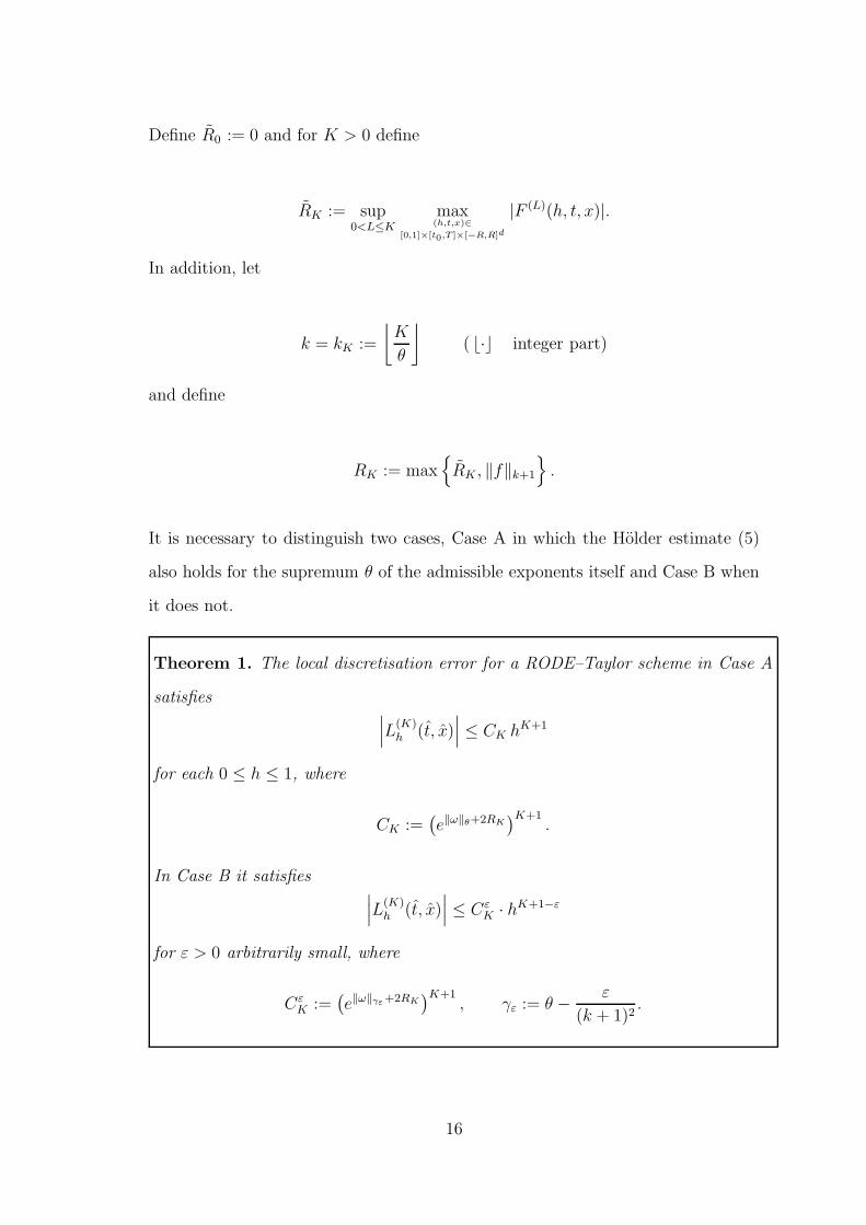
Theorem 1. The local discretisation error for a RODE–Taylor scheme in Case A
satisfies∣
∣
∣L
(K)h (t, x)
∣
∣
∣≤ CK hK+1
for each 0 ≤ h ≤ 1, where
CK :=(
e‖ω‖θ+2RK)K+1
.
In Case B it satisfies∣
∣
∣L
(K)h (t, x)
∣
∣
∣≤ Cε
K · hK+1−ε
for ε > 0 arbitrarily small, where
CεK :=
(
e‖ω‖γε+2RK)K+1
, γε := θ −ε
(k + 1)2.
16
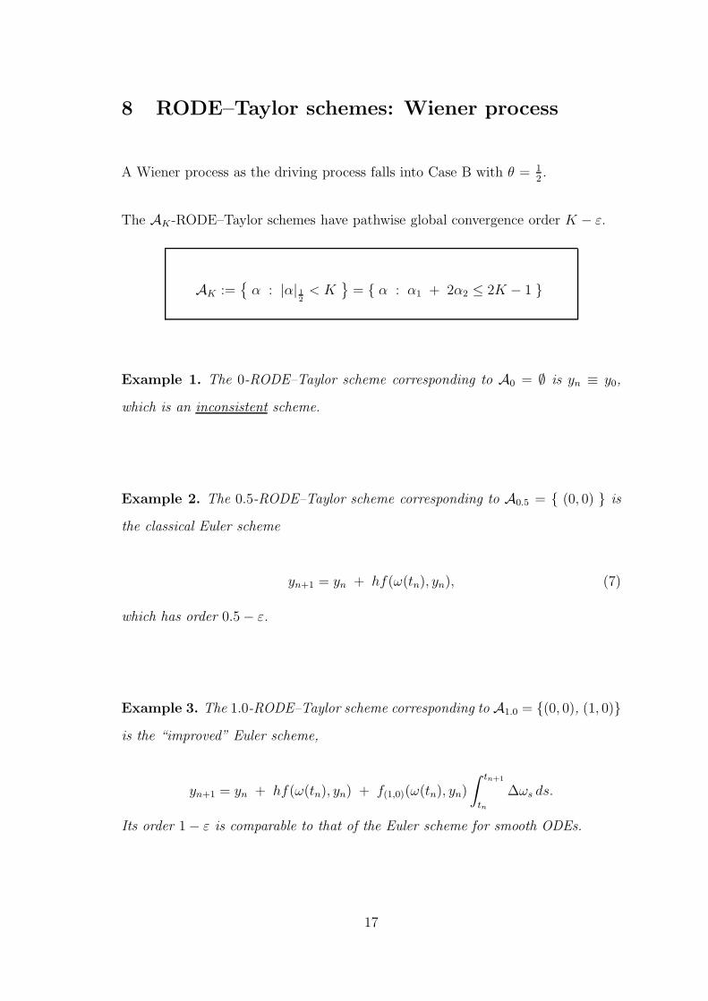
8 RODE–Taylor schemes: Wiener process
A Wiener process as the driving process falls into Case B with θ = 12.
The AK-RODE–Taylor schemes have pathwise global convergence order K − ε.
AK :=
α : |α| 12
< K
= α : α1 + 2α2 ≤ 2K − 1
Example 1. The 0-RODE–Taylor scheme corresponding to A0 = ∅ is yn ≡ y0,
which is an inconsistent scheme.
Example 2. The 0.5-RODE–Taylor scheme corresponding to A0.5 = (0, 0) is
the classical Euler scheme
yn+1 = yn + hf(ω(tn), yn), (7)
which has order 0.5 − ε.
Example 3. The 1.0-RODE–Taylor scheme corresponding to A1.0 = (0, 0), (1, 0)
is the “improved” Euler scheme,
yn+1 = yn + hf(ω(tn), yn) + f(1,0)(ω(tn), yn)
∫ tn+1
tn
∆ωs ds.
Its order 1 − ε is comparable to that of the Euler scheme for smooth ODEs.
17
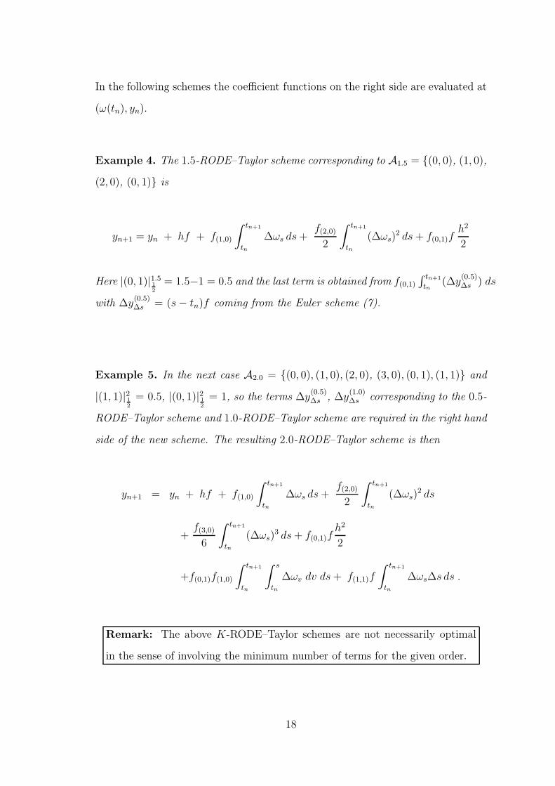
In the following schemes the coefficient functions on the right side are evaluated at
(ω(tn), yn).
Example 4. The 1.5-RODE–Taylor scheme corresponding to A1.5 = (0, 0), (1, 0),
(2, 0), (0, 1) is
yn+1 = yn + hf + f(1,0)
∫ tn+1
tn
∆ωs ds +f(2,0)
2
∫ tn+1
tn
(∆ωs)2 ds + f(0,1)f
h2
2
Here |(0, 1)|1.51
2
= 1.5−1 = 0.5 and the last term is obtained from f(0,1)
∫ tn+1
tn(∆y
(0.5)∆s ) ds
with ∆y(0.5)∆s = (s − tn)f coming from the Euler scheme (7).
Example 5. In the next case A2.0 = (0, 0), (1, 0), (2, 0), (3, 0), (0, 1), (1, 1) and
|(1, 1)|212
= 0.5, |(0, 1)|212
= 1, so the terms ∆y(0.5)∆s , ∆y
(1.0)∆s corresponding to the 0.5-
RODE–Taylor scheme and 1.0-RODE–Taylor scheme are required in the right hand
side of the new scheme. The resulting 2.0-RODE–Taylor scheme is then
yn+1 = yn + hf + f(1,0)
∫ tn+1
tn
∆ωs ds +f(2,0)
2
∫ tn+1
tn
(∆ωs)2 ds
+f(3,0)
6
∫ tn+1
tn
(∆ωs)3 ds + f(0,1)f
h2
2
+f(0,1)f(1,0)
∫ tn+1
tn
∫ s
tn
∆ωv dv ds + f(1,1)f
∫ tn+1
tn
∆ωs∆s ds .
Remark: The above K-RODE–Taylor schemes are not necessarily optimal
in the sense of involving the minimum number of terms for the given order.
18
9 Fractional Brownian motion
Fractional Brownian motion with Hurst exponent H = 34
also falls into Case B
with θ = 34. The RODE–Taylor schemes generally contain fewer terms than the
schemes of the same order with a Wiener process or attain a higher order when
they contain the same terms.
Example 6. For AK = (0, 0) with K ∈ (0, 34] the RODE–Taylor scheme is the
classical Euler scheme in Example 2, but now the order is 34− ε.
Example 7. AK = (0, 0), (1, 0) for K ∈ (34, 1] : the RODE–Taylor scheme is
the same as that in Example 3 and also has order 1 − ε.
Example 8. , For AK = (0, 0), (1, 0), (0, 1) with K ∈ (1, 32] the RODE–Taylor
scheme,
yn+1 = yn + hf + f(1,0)
∫ tn+1
tn
∆ωs + f(0,1)fh2
2,
which has order 1.5−ε, omits one of the terms in the RODE–Taylor scheme of the
same order for a Wiener process given in Example 4.
Example 9. For AK = (0, 0), (1, 0), (0, 1), (2, 0) with K ∈ (32, 7
4] the RODE–
Taylor scheme is the same as that for a Wiener process case in Example 4, but
now has order 74− ε instead of order order 3
2− ε.
19
Lecture 3: Stochastic Ordinary Differential
Equations
Deterministic calculus is much more robust to approximation than Ito stochas-
tic calculus because the integrand function in a Riemann sum approximating a
Riemann integral can be evaluated at an arbitrary point of the discretisation
subinterval, whereas for an Ito stochastic integral the integrand function must
always be evaluated at the left hand endpoint.
Consequently, considerable care is needed in deriving numerical schemes for
stochastic ordinary differential equations (SODEs) to ensure that they are con-
sistent with Ito calculus.
In particular, stochastic Taylor schemes are the essential starting point for the
derivation of consistent higher order numerical schemes for SODEs.
Other types of schemes for SODEs, such as derivative–free schemes, can then be
obtained by modifying the corresponding stochastic Taylor schemes.
1
1 Ito SODEs
Consider a scalar Ito stochastic differential equation (SODE)
dXt = a(t, Xt) dt + b(t, Xt) dWt, (1)
where (Wt)t∈R+ is a standard Wiener process, i.e., with W0 = 0, w.p.1, and incre-
ments Wt−Ws ∼ N(0; t−s) for t ≥ s ≥ 0, which are independent on nonoverlapping
subintervals.
The SODE (1) is, in fact, only symbolic for the stochastic integral equation
Xt = Xt0 +
∫ t
t0
a(s, Xs) ds +
∫ t
t0
b(s, Xs) dWs, (2)
where the first integral is pathwise a deterministic Riemann integral and the second
is an Ito stochastic integral — it is not a pathwise Riemann–Stieltjes integral !
The Ito stochastic integral of a nonanticipative mean–square integrable integrand
g is defined in terms of the mean–square limit, namely,
∫ T
t0
g(s) dWs := m.s. − lim∆→0
NT −1∑
n=0
g(tn, ω)
Wtn+1(ω) − Wtn(ω)
,
taken over partitions of [t0, T ] of maximum step size ∆ := maxn ∆n, where ∆n =
tn+1 − tn and tNT= T .
Two very useful properties of Ito integrals are
E
(∫ T
t0
g(s) dWs
)
= 0, E
(∫ T
t0
g(s) dWs
)2
=
∫ T
t0
Eg(s)2 ds.
2
2 Existence and uniqueness of strong solutions
The following is a standard existence and uniqueness theorem for SODEs. The
vector valued case is analogous.
Theorem 1. Supose that a, b : [t0, T ]× R → R are continuous in (t, x)
and satisfy the global Lipschitz condition
|a(t, x) − a(t, y)| + |b(t, x) − b(t, y)| ≤ L|x − y|
uniformly in t ∈ [t0, T ] and suppose that the random variable X0 is
nonanticipative with respect to the Wiener process Wt with
E(X20 ) < ∞.
Then the Ito SODE
dXt = a(t, Xt) dt + b(t, Xt) dWt
has a unique strong solution on [t0, T ] with initial value Xt0 = X0.
Alternatively, one could assume just a local Lipschitz condition. Then, the addi-
tional linear growth condition
|a(t, x)| + |b(t, x)| ≤ K(1 + |x|)
ensures the existence of the solution on the entire time interval [0, T ], i.e., prevents
explosions of solutions in finite time.
P.E. Kloeden and E. Platen, Numerical Solutions of Stochastic Differential
Equations, Springer-Verlag, Berlin Heidelberg New York, 1992.
3
3 Simple numerical schemes for SODEs
The counterpart of the Euler scheme for the SODE (1) is the Euler–Maruyama scheme
Yn+1 = Yn + a(tn, Yn) ∆n + b(tn, Yn) ∆Wn, (3)
with time and noise increments
∆n = tn+1 − tn =
∫ tn+1
tn
ds, ∆Wn = Wtn+1− Wtn =
∫ tn+1
tn
dWs.
It seems to be (and is) consistent with the Ito stochastic calculus because the noise
term in (3) approximates the Ito stochastic integral in (2) over a discretisation
subinterval [tn, tn+1] by evaluating its integrand at the left hand end point:
∫ tn+1
tn
b(s, Xs) dWs ≈
∫ tn+1
tn
b(tn, Xtn) dWs = b(tn, Xtn)
∫ tn+1
tn
dWs.
It is usual to distinguish between strong and weak convergence, depending on whether
the realisations or only their probability distributions are required to be close.
Let ∆ be the maximum step size of a given partition of a fixed interval [t0, T ]. A
numerical scheme is said to converge with strong order γ if
E
(∣
∣
∣XT − Y
(∆)NT
∣
∣
∣
)
≤ KT ∆γ (4)
and with weak order β if, for each polynomial g,
∣
∣
∣E (g(XT )) − E
(
g(Y(∆)NT
))∣
∣
∣≤ Kg,T ∆β (5)
• The Euler–Maruyama scheme (3) has strong order γ = 12, weak order β = 1.
4
To obtain a higher order, one should avoid heuristic adaptations of well known
deterministic numerical schemes because they are usually inconsistent with Ito
calculus or, when consistent, do not improve the order of convergence.
Example: The deterministic Heun scheme adapted to the Ito SODE (1) has the
form
Yn+1 = Yn +1
2[a(tn, Yn) + a(tn+1, Yn + a(tn, Yn)∆n + b(tn, Yn)∆Wn)] ∆n
+1
2[b(tn, Yn) + b(tn+1, Yn + a(tn, Yn)∆n + b(tn, Yn)∆Wn)] ∆Wn.
For the Ito SODE dXt = Xt dWt it simplifies to
Yn+1 = Yn +1
2Yn (2 + ∆Wn) ∆Wn.
The conditional expectation
E
(
Yn+1 − Yn
∆n
∣
∣
∣
∣
Yn = x
)
=x
∆n
E
(
∆Wn +1
2(∆Wn)2
)
=x
∆n
(
0 +1
2∆n
)
=1
2x
should approximate the drift term a(t, x) ≡ 0 of the SODE. The adapted Heun
scheme is thus not consistent with Ito calculus and does not converge in either the
weak or strong sense.
To obtain a higher order of convergence one needs to provide more information
about the Wiener process within the discretisation subinterval than that provided
by the simple increment ∆Wn.
Such information is provided by multiple integrals of the Wiener process, which
arise in stochastic Taylor expansions of the solution of an SODE.
• Consistent numerical schemes of arbitrarily desired higher order can be derived
by truncating appropriate stochastic Taylor expansions.
5
4 Ito–Taylor expansions
Ito–Taylor expansions or stochastic Taylor expansions of solutions of Ito SODEs are
derived through an iterated application of the stochastic chain rule, the Ito formula.
The nondifferentiability of the solutions in time is circumvented by using the integral
form of the Ito formula.
The Ito formula for scalar valued function f(t, Xt) of the solution Xt of the scalar
Ito SODE (1) is
f(t, Xt) = f(t0, Xt0) +
∫ t
t0
L0f(s, Xs) ds +
∫ t
t0
L1f(s, Xs) dWs, (6)
where the operators L0 and L1 are defined by
L0 =∂
∂t+ a
∂
∂x+
1
2b2 ∂2
∂x2 , L1 = b∂
∂x.
This differs from the deterministic chain rule by the additional third term in the
L0 operator, which is due to the fact that E (|∆W |2) = ∆t.
When f(t, x) ≡ x, the Ito formula (6) is just the integral version (2) of the SODE
(1) in the integral form
Xt = Xt0 +
∫ t
t0
a(s, Xs) ds +
∫ t
t0
b(s, Xs) dWs. (7)
6

Iterated application of the Ito formula
Applying the Ito formula to the integrand functions
f(t, x) = a(t, x), f(t, x) = b(t, x)
in the SODE (7) gives
Xt = Xt0 +
∫ t
t0
[
a(t0, Xt0) +
∫ s
t0
L0a(u, Xu) du +
∫ s
t0
L1a(u, Xu) dWu
]
ds
+
∫ t
t0
[
b(t0, Xt0) +
∫ s
t0
L0b(u, Xu) du +
∫ s
t0
L1b(u, Xu) dWu
]
dWs.
= Xt0 + a(t0, Xt0)
∫ t
t0
ds + b(t0, Xt0)
∫ t
t0
dWs + R1(t, t0) (8)
with the remainder
R1(t, t0) =
∫ s
t0
∫ s
t0
L0a(u, Xu) du ds +
∫ s
t0
∫ s
t0
L1a(u, Xu) dWu ds
+
∫ t
t0
∫ s
t0
L0b(u, Xu) du dWs +
∫ t
t0
∫ s
t0
L1b(u, Xu) dWu dWs.
Discarding the remainder gives the simplest stochastic Taylor approximation
Xt ≈ Xt0 + a(t0, Xt0)
∫ t
t0
ds + b(t0, Xt0)
∫ t
t0
dWs,
which has strong order γ = 0.5 and weak order β = 1.
• Higher order stochastic Taylor expansions are obtained by applying the Ito
formula to selected integrand functions in the remainder.
7
e.g., to the integrand L1b in the fourth double integral of the remainder R1(t, t0)
gives the stochastic Taylor expansion
Xt = Xt0 + a(t0, Xt0)
∫ t
t0
ds + b(t0, Xt0)
∫ t
t0
dWs
+L1b(t0, Xt0)
∫ t
t0
∫ s
t0
dWu dWs + R2(t, t0) (9)
with the remainder
R2(t, t0) =
∫ s
t0
∫ s
t0
L0a(u, Xu) du ds +
∫ s
t0
∫ s
t0
a(u, Xu) dWu ds
+
∫ t
t0
∫ s
t0
L0b(u, Xu) du dWs +
∫ t
t0
∫ s
t0
∫ u
t0
L0L1b(v, Xv) dv dWu dWs
+
∫ t
t0
∫ s
t0
∫ u
t0
L1L1b(v, Xv) dWv dWu dWs.
Discarding the remainder gives the stochastic Taylor approximation
Xt ≈ Xt0 + a(t0, Xt0)
∫ t
t0
ds + b(t0, Xt0)
∫ t
t0
dWs
+ b(t0, Xt0)∂b
∂x(t0, Xt0)
∫ t
t0
∫ s
t0
dWu dWs,
since L1b = b∂b
∂x. This has strong order γ = 1 (and also weak order β = 1).
Remark: These two examples already indicate the general pattern of the schemes:
i) they achieve their higher order through the inclusion of multiple stochastic integral
terms;
ii) an expansion may have different strong and weak orders of convergence;
iii) the possible orders for strong schemes increase by a fraction 12, taking values 1
2,
1, 32, 2, . . ., whereas possible orders for weak schemes are whole numbers 1, 2, 3, . . ..
8
5 General stochastic Taylor expansions
Multi–indices provide a succinct means to describe the terms that should be included
or expanded to obtain a stochastic Taylor expansion of a particular order as well
as for representing the iterated differential operators and stochastic integrals that
appear in the terms of such expansions.
A multi–index α of length l(α) = l is an l-dimensional row vector α = (j1, j2, . . . , jl)
∈ 0, 1l with components ji ∈ 0, 1 for i ∈ 1, 2, . . ., l.
Let M1 be the set of all multi–indices of length greater than or equal to zero, where
a multi–index ∅ of length zero is introduced for convenience.
Given a multi–index α ∈ M1 with l(α) ≥ 1, write −α and α− for the multi–index
in M1 obtained by deleting the first and the last component, respectively, of α.
For a multi–index α = (j1, j2, . . ., jl) with l ≥ 1, define the multiple Ito integral
recursively by (here W 0t = t and W 1
t = Wt)
Iα[g(·)]t0,t :=
∫ t
t0
Iα−[g(·)]t0,s dW jls , I∅[g(·)]t0,t := g(t)
and the Ito coefficient function for a deterministic function f recursively by
fα := Lj1f−α, f∅ = f.
9
The multiple stochastic integrals appearing in a stochastic Taylor expansion with
constant integrands cannot be chosen completely arbitrarily.
The set of corresponding multi–indices must form an hierarchical set, i.e., a nonempty
subset A of M1 with
supα∈A
l(α) < ∞ and − α ∈ A for each α ∈ A \ ∅.
The multi–indices of the remainder terms in a stochastic Taylor expansion for a
given hierarchical set A belong to the corresponding remainder set B(A) of A
defined by
B(A) = α ∈ M1 \ A : −α ∈ A,
i.e., consisting of all of the “next following” multi–indices with respect to the given
hierarchical set.
The Ito–Taylor expansion for the hierarchical set A and remainder set B(A) is
f(t, Xt) =∑
α∈A
fα(t0, Xt0) Iα [1]t0,t +∑
α∈B(A)
Iα [fα(·, X·)]t0,t ,
i.e., with constant integrands (hence constant coefficients) in the first sum and time
dependent integrands in the remainder sum.
10
6 Ito–Taylor Numerical Schemes for SODEs
Ito–Taylor numerical schemes are obtained by applying Ito–Taylor expansion to the
identity function f = id on a subinterval [tn, tn+1] at a starting point (tn, Yn) and
discarding the remainder term.
The Ito-Taylor expansion (8) gives the Euler–Maruyama scheme (3), which is the
simplest nontrivial stochastic Taylor scheme. It has strong order γ = 0.5 and weak
order β = 1.
The Ito–Taylor expansion (9) gives the Milstein scheme
Yn+1 = Yn + a(tn, Yn) ∆n + b(tn, Yn) ∆Wn
+ b(tn, Yn)∂b
∂x(tn, Xn)
∫ tn+1
tn
∫ s
tn
dWu dWs.
Here the coefficient functions are f(0) = a, f(1) = b, f(1,1) = b∂b
∂xand the iterated
integrals
I(0)(tn, tn+1) =
∫ tn+1
tn
dW 0s = ∆n, I(1)(tn, tn+1) =
∫ tn+1
tn
dW 1s = ∆Wn,
and
I(1,1)(tn, tn+1) =
∫ tn+1
tn
∫ s
tn
dW 1τ dW 1
s =1
2
[
(∆Wn)2 − ∆n
]
. (10)
The Milstein scheme converges with strong order γ = 1 and weak order β = 1.
It has a higher order of convergence in the strong sense than the Euler–Maruyama
scheme, but gives no improvement in the weak sense.
11
Applying this idea to the Ito–Taylor expansion corresponding to the hierarchical
set A gives the A-stochastic Taylor scheme
Y An+1 =
∑
α∈A
Iα
[
idα(tn, Y An )
]
tn,tn+1
= Y An +
∑
α∈A\∅
idα(tn, Y An ) Iα [1]tn,tn+1
.
(11)
The strong order γ stochastic Taylor scheme, which converges with strong order γ,
involves the hierarchical set
Λγ =
α ∈ Mm : l(α) + n(α) ≤ 2γ or l(α) = n(α) = γ +1
2
,
where n(α) denotes the number of components of a multi–index α equal to 0.
The weak order β stochastic Taylor scheme, which converges with weak order β,
involves the hierarchical set
Γβ = α ∈ Mm : l(α) ≤ β .
For example, the hierarchical sets Λ1/2 = Γ1 = ∅, (0), (1) give the stochastic
Euler–Maruyama scheme, which is both strongly and weakly convergent, while
the strongly convergent Milstein scheme corresponds to the hierarchical set Λ1 =
∅, (0), (1), (1, 1).
• The Milstein scheme does not correspond to a stochastic Taylor scheme for an
hierarchical set Γβ.
12
0 0
1
0
1
0
0
1
1
0
1
0
1
0
0
1
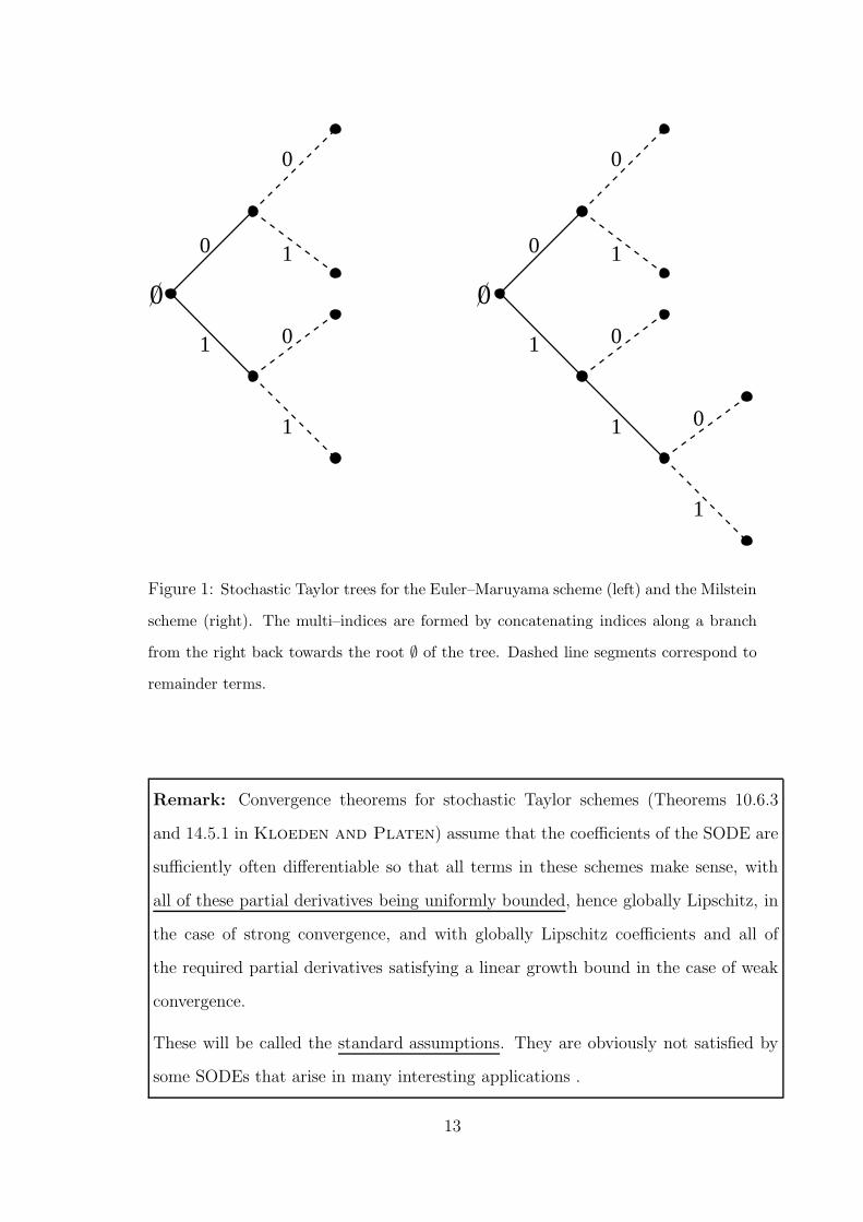
Figure 1: Stochastic Taylor trees for the Euler–Maruyama scheme (left) and the Milstein
scheme (right). The multi–indices are formed by concatenating indices along a branch
from the right back towards the root ∅ of the tree. Dashed line segments correspond to
remainder terms.
Remark: Convergence theorems for stochastic Taylor schemes (Theorems 10.6.3
and 14.5.1 in Kloeden and Platen) assume that the coefficients of the SODE are
sufficiently often differentiable so that all terms in these schemes make sense, with
all of these partial derivatives being uniformly bounded, hence globally Lipschitz, in
the case of strong convergence, and with globally Lipschitz coefficients and all of
the required partial derivatives satisfying a linear growth bound in the case of weak
convergence.
These will be called the standard assumptions. They are obviously not satisfied by
some SODEs that arise in many interesting applications .
13
7 Pathwise convergence
Pathwise convergence was already considered for RODEs and is also interesting for
SODEs because numerical calculations of the random variables Yn in the numerical
scheme above are carried out path by path.
Ito stochastic calculus is, however, an L2 or a mean–square calculus and not a path-
wise calculus.
Given that the sample paths of a Wiener process are Holder continuous with ex-
ponent 12− ǫ one may ask:
Is the convergence order 12− ǫ “sharp” for pathwise approximation?
The answer is no! An arbitrary pathwise convergence order is possible.
P.E. Kloeden and A. Neuenkirch, The pathwise convergence of approximation
schemes for stochastic differential equations, LMS J. Comp. Math. 10 (2007)
Theorem 2. Under the standard assumptions the Ito–Taylor scheme of strong order
γ > 0 converges pathwise with order γ − ǫ for all ǫ > 0, i.e.,
supi=0,...,NT
∣
∣Xtn(ω) − Y (γ)n (ω)
∣
∣ ≤ K(γ)ǫ,T (ω) · ∆γ−ǫ
for almost all ω ∈ Ω.
Note that the error constant here depends on ω, so it is in fact a random variable.
The nature of its statistical properties is an interesting question, about which little
is known theoretically so far and requires further investigation.
14
The proof of Theorem 2 is based on the Burkholder–Davis–Gundy inequality
E sups∈[0,t]
∣
∣
∣
∣
∫ s
0
Xτ dWτ
∣
∣
∣
∣
p
≤ Cp · E
∣
∣
∣
∣
∫ t
0
X2τ dτ
∣
∣
∣
∣
p/2
and a Borel–Cantelli argument in the following lemma.
Lemma 1. Let γ > 0 and cp ≥ 0 for p ≥ 1. If Znn∈N is a sequence of random
variables with
(E|Zn|p)
1/p ≤ cp · n−γ
for all p ≥ 1 and n ∈ N, then for each ǫ > 0 there exists a non–negative random
variable Kǫ such that
|Zn(ω)| ≤ Kǫ(ω) · n−γ+ε, a.s.,
for all n ∈ N.
15
8 Restrictiveness of the standard assumptions
Proofs in the literature of the convergence orders of Ito–Taylor schemes assume that
the coefficient functions fα are uniformly bounded on R1, i.e., the partial deriva-
tives of appropriately high order of the SODE coefficient functions a and b are
uniformly bounded on R1.
This assumption is not satisfied for many SODEs in important applications such
as:
• the stochastic Ginzburg–Landau equation
dXt =
((
ν +1
2σ2
)
Xt − λX3t
)
dt + σXt dWt.
Matters are even worse for
• the Fisher–Wright equation
dXt = [κ1(1 − Xt) − κ2Xt] dt +√
Xt(1 − Xt) dWt
• the Feller diffusion with logistic growth SODE
dXt = λXt (K − Xt) dt + σ√
Xt dWt
• the Cox–Ingersoll–Ross equation
dVt = κ (λ − Vt) dt + θ√
Vt dWt,
since the square root function is not differentiable at zero and requires the expres-
sion under it to remain non–negative for the SODE to make sense.
16
9 Counterexample: Euler–Maruyama scheme
The scalar SODE
dXt = −X3t dt + dWt
with the cubic drift and additive noise has a globally pathwise asymptotically stable
stochastic stationary solution. Its solution on the time interval [0, 1] for initial value
X0 = 0 satisfies the stochastic integral equation
Xt = −
∫ t
0
X3s ds + Wt (12)
and has finite first moment E |X1| < ∞ at T = 1.
The corresponding Euler–Maruyama scheme with constant step size ∆ = 1N
is given
by
Y(N)k+1 = Y
(N)k −
(
Y(N)k
)3
∆ + ∆Wk(ω).
This scheme does not converge either strongly or weakly.
M. Hutzenthaler, A. Jentzen and P.E. Kloeden, Strong and weak diver-
gence in finite time of Euler’s method for SDEs with non-globally Lipschitz coeffi-
cients, (submitted).
Theorem 3. The solution Xt of (12) and its Euler–Maruyama approximation Y(N)k
satisfy
limN→∞
E
∣
∣
∣X1 − Y
(N)N
∣
∣
∣= ∞. (13)
17
Outline of proof
Let N ∈ N be arbitrary, define rN := max 3N, 2 and consider the event
ΩN :=
ω ∈ Ω : supk=1,...,N−1
|∆Wk(ω)| ≤ 1, |∆W0(ω)| ≥ rN
.
Then, it follows by induction that
∣
∣
∣Y
(N)k (ω)
∣
∣
∣≥ r2k−1
N , ∀ ω ∈ ΩN ,
for every k = 1, 2, . . . , N .
P [ΩN ] = P
[
supk=1,...,N−1
|∆Wk| ≤ 1
]
· P [|∆W0| ≥ rN ]
≥ P
[
sup0≤t≤1
|Wt| ≤1
2
]
· P [|∆W0| ≥ rN ]
= P
[
sup0≤t≤1
|Wt| ≤1
2
]
· P
[√N
∣
∣W1/N
∣
∣ ≥√
NrN
]
≥ P
[
sup0≤t≤1
|Wt| ≤1
2
]
·1
4
√NrNe−(
√NrN )2
≥1
4· P
[
sup0≤t≤1
|Wt| ≤1
2
]
· e−Nr2
N
for every N ∈ N. It follows that
limN→∞
E
∣
∣
∣Y
(N)N
∣
∣
∣≥
1
4· P
[
sup0≤t≤1
|Wt| ≤1
2
]
· limN→∞
e−Nr2
N · 22N−1
=1
4· P
[
sup0≤t≤1
|Wt| ≤1
2
]
· limN→∞
e−9N3
· 22N−1
= ∞.
Finally, since E |X1| is finite,
limN→∞
E
∣
∣
∣X1 − Y
(N)N
∣
∣
∣≥ lim
N→∞E
∣
∣
∣Y
(N)N
∣
∣
∣− E |X1| = ∞.
18
Lecture 4: SODEs: Nonstandard Assumptions
There are various ways to overcome the problems caused by nonstandard
assumptions on the coefficients of an SODE.
One way is to restrict attention to SODEs with special dynamical properties
such as ergodicity, e.g., by assuming that the coefficients satisfy certain
dissipativity and nondegeneracy conditions.
This yields the appropriate order estimates without bounded derivatives of
coefficients.
However, several type of SODEs and in particular SODEs with square root
coefficients remain a problem.
Many numerical schemes do not preserve the domain of the solution of the
SODE and hence may crash when implemented, which has led to various
ad hoc modifications to prevent this from happening.
Pathwise and Monte Carlo convergences often have to be used instead of
strong and weak convergences.
1
1 SODEs without uniformly bounded coefficients
A localisation argument was used by
A. Jentzen, P.E. Kloeden and A. Neuenkirch, Convergence of numerical
approximations of stochastic differential equations on domains: higher order con-
vergence rates without global Lipschitz coefficients, Numerische Mathematik 112
(2009), no. 1, 41–64.
to show that the convergence theorem for strong Taylor schemes remains true for
an SODE
dXt = a(Xt) dt + b(Xt) dWt
when the coefficients satisfy
a, b ∈ C2γ+1(R1; R1),
i.e., they do not necessarily have uniformly bounded derivatives.
The convergence obtained is pathwise. This is a special case of Theorem 1 below.
Pathwise convergence with order γ − ǫ where ǫ > 0:
supi=0,...,N
∣
∣Xtn(ω) − Y (γ)n (ω)
∣
∣ ≤ K(γ)ǫ (ω) · ∆γ−ǫ
for almost all ω ∈ Ω.
Whether a strong convergence rate can always be derived under these assumptions
remains an open problem.
2
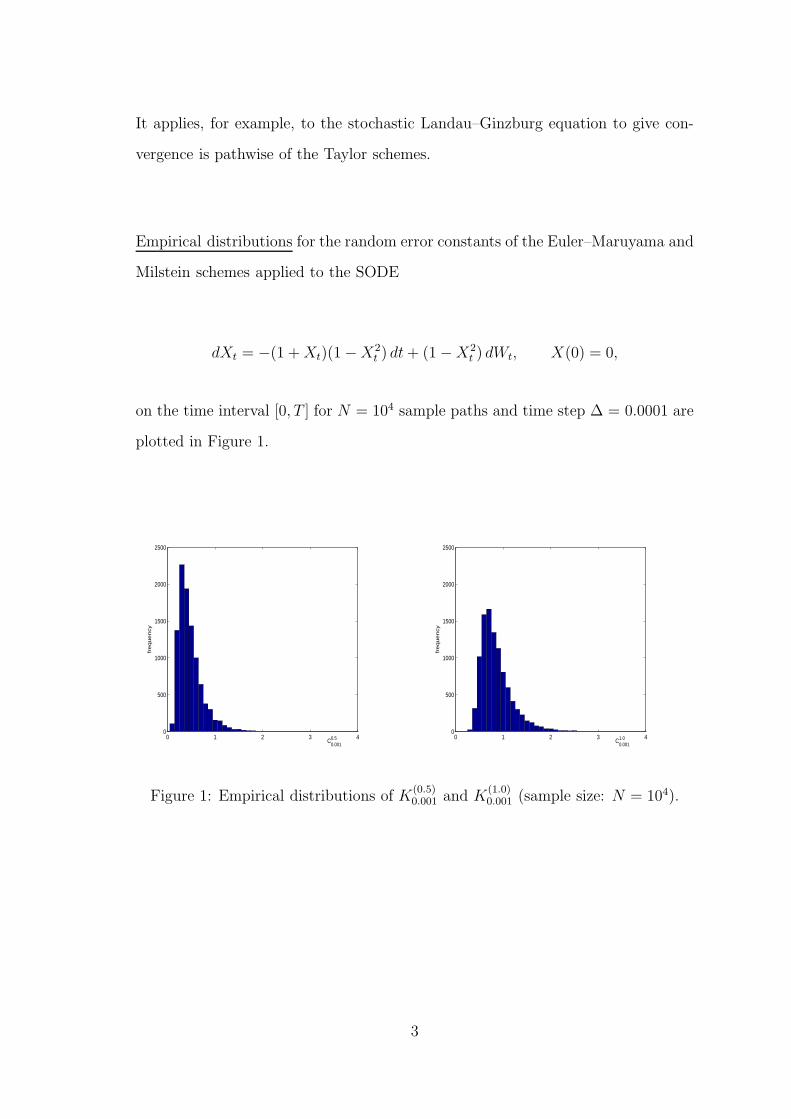
It applies, for example, to the stochastic Landau–Ginzburg equation to give con-
vergence is pathwise of the Taylor schemes.
Empirical distributions for the random error constants of the Euler–Maruyama and
Milstein schemes applied to the SODE
dXt = −(1 + Xt)(1 − X2t ) dt + (1 − X2
t ) dWt, X(0) = 0,
on the time interval [0, T ] for N = 104 sample paths and time step ∆ = 0.0001 are
plotted in Figure 1.
0 1 2 3 40
500
1000
1500
2000
2500
C0.50.001
fre
qu
en
cy
0 1 2 3 40
500
1000
1500
2000
2500
C1.00.001
fre
qu
en
cy
Figure 1: Empirical distributions of K(0.5)0.001 and K
(1.0)0.001 (sample size: N = 104).
3
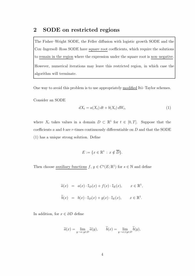
2 SODE on restricted regions
The Fisher–Wright SODE, the Feller diffusion with logistic growth SODE and the
Cox–Ingersoll–Ross SODE have square root coefficients, which require the solutions
to remain in the region where the expression under the square root is non–negative.
However, numerical iterations may leave this restricted region, in which case the
algorithm will terminate.
One way to avoid this problem is to use appropriately modified Ito–Taylor schemes.
Consider an SODE
dXt = a(Xt) dt + b(Xt) dWt, (1)
where Xt takes values in a domain D ⊂ R1 for t ∈ [0, T ]. Suppose that the
coefficients a and b are r-times continuously differentiable on D and that the SODE
(1) has a unique strong solution. Define
E := x ∈ R1 : x /∈ D.
Then choose auxiliary functions f , g ∈ Cs(E; R1) for s ∈ N and define
a(x) = a(x) · ID(x) + f(x) · IE(x), x ∈ R1,
˜b(x) = b(x) · ID(x) + g(x) · IE(x), x ∈ R1.
In addition, for x ∈ ∂D define
a(x) = limy→x; y∈D
a(y), ˜b(x) = limy→x;∈y∈D
˜b(y),
4
and the “modified” derivative of a function h : R1 → R
1 by
∂xlh(x) =∂
∂xlh(x), x ∈ D ∪ E,
∂xlh(x) = limy→x; y∈D
∂xlh(x), l = 1, . . . , d, x ∈ ∂D.
If the above limits do not exist, set a(x) = 0, ˜b(x) = 0 and ∂xlh(x) = 0 for x ∈ ∂D.
A modified Ito–Taylor scheme is the corresponding Ito–Taylor scheme for the SODE
with modified coefficients
dXt = a(Xt) dt +˜b(Xt) dWt, (2)
The purpose of the auxiliary functions is twofold:
• to obtain a well defined approximation scheme
• to “reflect” the numerical scheme back into D after it has left D.
Theorem 1. Assume that a, ˜b ∈ C2γ+1(D; R1)⋂
C2γ−1(E; R1).
Then, for every ǫ > 0 and γ = 12, 1, 3
2, . . . there exists a non–negative random
variable K(f,g)γ,ǫ such that
supn=0,...,NT
∣
∣Xtn(ω) − Y (mod,γ)n (ω)
∣
∣ ≤ K(f,g)γ,ǫ (ω) · ∆γ−ǫ
for almost all ω ∈ Ω and all n = 1, . . ., NT , where ∆ = T/NT and the Y(mod,γ)n
correspond to the modified Ito–Taylor scheme applied to the SODE (2).
The convergence rate does not depend on the choice of the auxiliary functions, but
the random constant in the error bound clearly does.
5
3 Examples
Example 1
Consider the Cox–Ingersoll–Ross SODE
dXt = κ (λ − Xt) dt + θ√
Xt dWt
with κλ ≥ θ2/2 and x(0) = x0 > 0.
Here D = (0,∞) and the coefficients
a(x) = κ (λ − x) , b(x) = θ√
x, x ∈ D,
satisfy a, b ∈ C∞(D; R1).
As auxiliary functions on E = = (−∞, 0) choose, e.g.,
f(x) = g(x) = 0, x ∈ E,
or
f(x) = κ (λ − x) , g(x) = 0, x ∈ E.
The first choice of auxiliary functions “kills” the numerical approximation as soon
as it reaches a negative value.
However, the second is more appropriate, since if the scheme would take a negative
value, the auxiliary functions force the numerical scheme to be positive again after
the next steps, which recovers better the positivity of the exact solution.
6

Example 2
A general version of the Wright–Fisher SODE
dXt = f(Xt) dt +√
Xt(1 − Xt) dWt (3)
typically has a polynomial drift coefficient f .
Its solution should take values in the interval [0, 1], but, in general, depending on
the structure of f , the solution can attain the boundary 0, 1 in finite time, i.e.,
τ0,1 = inft ∈ [0, T ] : Xt /∈ (0, 1) < T
almost surely. Thus, Theorem 1 cannot be applied directly to the SODE (3).
But a modified Ito–Taylor method Y(mod,γ)n with the auxiliary functions f = 0 and
g = 0 to (3) can be used up to the first hitting time of the boundary of D.
The error bound then takes the form
supi=0,...,n
∣
∣
∣Yti(ω) − Y
(mod,γ)i (ω)
∣
∣
∣≤ ηγ,ǫ(ω) · n−γ+ǫ
for almost all ω ∈ Ω and all n ∈ N, where
Yti(ω) = Xt(ω) IXt(ω)∈(0,1), t ≥ 0, ω ∈ Ω.
7
4 Monte Carlo convergence
The concepts of strong and weak convergence of a numerical scheme are theoretical
discretisation concepts.
In practice, one has to estimate the expectations by a finite random sample.
In the weak case, neglecting roundoff and other computational errors, one uses in
fact the convergence
limN,M→∞
∣
∣
∣
∣
∣
E
[
g(
XT
)
]
−1
M
M∑
k=1
g(
Y(N)N (ωk)
)
∣
∣
∣
∣
∣
= 0 (4)
for smooth functions g : R → R with derivatives having at most polynomial growth.
By the triangle inequality
∣
∣
∣
∣
∣
E
[
g(
XT
)
]
−1
M
M∑
k=1
g(
Y(N)N (ωk)
)
∣
∣
∣
∣
∣
≤∣
∣
∣E
[
g(
XT
)
]
− E
[
g(
Y(N)N
)
]∣
∣
∣+
∣
∣
∣
∣
∣
E
[
g(
Y(N)N
)
]
−1
M
M∑
k=1
g(
Y(N)N (ωk)
)
∣
∣
∣
∣
∣
.
where the first and second summands on the right hand side are, respectively,
• the weak discretisation error due to approximating the exact solution with
numerical
• the statistical error due to approximating an expectation with the arithmetic
average of finitely many independent samples.
8
Thus, if the numerical scheme converges weakly, then it also converges in the above
sense (4), which was called Monte Carlo convergence in
M. Hutzenthaler and A. Jentzen, Convergence of the stochastic Euler scheme
for locally Lipschitz coefficients, (submitted).
Monte Carlo convergence often holds for the Euler–Maruyama scheme applied to
a scalar SODE such as
dXt = −X3t dt + dWt, X0 = 0,
for which neither strong nor weak convergence holds.
The sample mean 1M
∑M
k=1 g(
Y(N)N (ωk)
)
in (4) is, in fact, a random variable, so the
Monte Carlo convergence (4) should be interpreted as holding almost surely.
To formulate this in a succinct way, the sample paths of M independent Wiener
processes W(1)t (ω), . . ., W
(M)t (ω) for the same ω will be considered instead of M
different sample paths Wt(ω1), . . ., Wt(ωM) of the same Wiener process Wt.
• The choice M = N2 ensures that Monte Carlo convergence for the Euler–
Maruyama scheme has the same order as that for weak convergence under standard
assumptions, namely 1, since the Monte Carlo simulation of E[
g(
Y(N)N
)]
with M
independent Euler approximations has convergence order 12− ǫ for an arbitrarily
small ǫ > 0.
With these modifications, Monte Carlo convergence takes the form
limN→∞
∣
∣
∣
∣
∣
E
[
g(
XT
)
]
−1
N2
N2
∑
k=1
g(
Y(N,k)N (ω)
)
∣
∣
∣
∣
∣
= 0, a.s., (5)
where Y(N,k)N (ω) is the ω-realisation of the Nth iterate of the Euler–Maruyama
scheme applied to the SODE with the ω-realisation of the kth Wiener process
W(k)t (ω).
9
Let (Ω,F , P) be a probability space.
Theorem 2. Suppose that a, b, g : R → R are four times continuously differentiable
functions with derivatives satisfying
∣
∣a(n)(x)∣
∣ +∣
∣b(n)(x)∣
∣ +∣
∣g(n)(x)∣
∣ ≤ L (1 + |x|r) , ∀x ∈ R,
for n = 0,1,. . . , 4, where L ∈ (0,∞) and r ∈ (1,∞) are fixed constants. Moreover,
suppose that the drift coefficient a satisfies the global one–sided Lipschitz condition
(x − y) · (a(x) − a(y)) ≤ L (x − y)2, ∀x, y ∈ R,
and that the diffusion coefficient satisfies the global Lipschitz condition
|b(x) − b(y)| ≤ L |x − y| , ∀x, y ∈ R.
Then, there is F-measurable mappings Cε : Ω → [0,∞) for each ε ∈ (0, 1) and an
event Ω ∈ F with P[Ω] = 1 such that
∣
∣
∣
∣
∣
E
[
g(XT )
]
−1
N2
(
N2
∑
m=1
g(Y(N,k)N (ω))
)∣
∣
∣
∣
∣
≤ Cε(ω) ·1
N1−ε
for every ω ∈ Ω, N ∈ N and ε ∈ (0, 1), where Xt is the solution of the SODE
dXt = a(Xt) dt + b(Xt) dWt
and Y(N,k)N is the N th iterate of the Euler–Maruyama scheme applied to this SODE
with the Wiener process W(k)t for k = 1, . . ., N2.
10
Lecture 5: Stochastic Partial Differential
Equations
The stochastic partial differential equations (SPDEs) considered here are stochastic
evolution equations of the parabolic or hyperbolic types.
There is an extensive literature on SPDEs.
P.L. Chow, Stochastic Partial Differential Equations, Chapman & Hall/CRC,
Boca Raton, 2007.
G. Da Prato and G. Zabczyk, Stochastic Equations in Infinite Dimensions,
Cambridge University Press, Cambridge, 1992.
W. Grecksch and C. Tudor, Stochastic Evolution Equations. A Hilbert Space
Approach, Akademie–Verlag, Berlin, 1995.
N.V. Krylov and B.L. Rozovskii, Stochastic Evolution Equations, World Sci.
Publ., Hackensack, N.J., 2007.
C. Prevot and M. Rockner, A Concise Course on Stochastic Partial Differ-
ential Equations, Springer–Verlag, Berlin, 2007.
The theory of such SPDEs is complicated by different types of solution concepts and
function spaces depending on the spatial regularity of the driving noise process.
1
1 Random and stochastic PDEs
As with RODEs and SODEs, one can distinguish between random and stochastic
partial differential equations.
Attention is restricted here to parabolic reaction–diffusion type equations on a
bounded spatial domain D in Rd with smooth boundary ∂D with a Dirichlet bound-
ary condition.
An example of a random PDE (RPDE) is
∂u
∂t= ∆u + f(ζt, u), u
∣
∣
∂D= 0,
where ζt is a stochastic process (possibly infinite dimensional). This is interpreted
and analysed pathwise as a deterministic PDE.
An example of an Ito stochastic PDE (SPDE) is
dXt = [∆Xt + f(Xt)] dt + g(Xt) dWt, Xt
∣
∣
∂D= 0, (1)
where Wt an infinite dimensional Wiener process of the form
Wt(x, ω) =
∞∑
k=1
ckWkt (ω)φk(x), t ≥ 0, x ∈ D,
with pairwise independent scalar Wiener processes W kt , k ∈ N, and an orthonormal
basis system (φk)k∈Nof some function space, e.g., L2(D).
As for SODEs, the theory of SPDEs is a mean–square theory and requires an
infinite dimensional version of Ito stochastic calculus.
2
The Doss–Sussmann theory is not as well developed for SPDEs as for SODEs,
but in simple cases an SPDE can be transformed to an RPDE.
For example, the SPDE (1) with additive noise
dXt = [∆Xt + f(Xt)] dt + dWt, Xt
∣
∣
∂D= 0,
is equivalent to the RPDE
∂v
∂t= ∆v + f(v + Ot) + Ot
with v(t) = Xt − Ot, t ≥ 0, where Ot is the (infinite-dimensional) Ornstein–
Uhlenbeck stochastic stationary solution of the linear SPDE
dOt = [∆Ot − Ot] dt + dWt, Ot
∣
∣
∂D= 0.
As a specific example, the RPDE with a scalar Ornstein–Uhlenbeck process,
∂v
∂t=
∂2v
∂x2− v − (v + Ot)
3
on the spatial interval 0 ≤ x ≤ 1 with Dirichlet boundary conditions is equivalent
to the SPDE with additive noise
dXt =
[
∂2
∂x2Xt − Xt − X3
t
]
dt + dWt
on D = [0, 1] with Dirichlet boundary conditions and a scalar Wiener process.
3
2 Mild solutions of SPDEs
An Ito stochastic partial differential equation (SPDE)
dXt = [AXt + F (Xt)] dt + B(Xt) dWt (2)
on a Hilbert space H , where
• A is, in general, an unbounded linear operator, e.g., the Laplace operator ∆
with the Dirichlet boundary condition
• (Wt)t∈R+ is an infinite dimensional cylindrical Wiener process,
is a stochastic integral equation
Xt = x0 +
∫ t
0
[AXs + F (Xs)] ds +
∫ t
0
B(Xs) dWs
on H , where the first integral is pathwise a deterministic integral and the second
an Ito stochastic integral in H .
There are several different interpretations of the stochastic integral equation (2) in
the literature.
The mild form is used here since it is better suited for the derivation of Taylor
expansions and numerical schemes.
The Ito stochastic integrals here and below are defined analogously to the
finite dimensional case.
4
The mild form of the SPDE (2) is also a stochastic integral equation in H
Xt = eAtx0 +
∫ t
0
eA(t−s)F (Xs) ds +
∫ t
0
eA(t−s)B(Xs) dWs, a.s., (3)
where(
eAt)
t≥0is a semigroup of solution operators of the deterministic ODE/PDE
dX
dt= AX ⇔
∂u
∂t= ∆u, u
∣
∣
∂D= 0,
on H , i.e., eAt = St for t ≥ 0, where X(t) = St(x0) is the solution with Dirichlet
boundary conditions for the initial value X(0) = x0.
In the finite dimensional case, H = Rd, the SPDE is an SODE, A is a d× d
matrix and eAt is a matrix exponential.
Define the Lq-norm of of a random variable Z : Ω → U , where U is a Hilbert space,
for q ≥ 1 by
|Z|Lq := (E|Z|qU)1
q
The following is a version of the Burkholder–Davis–Gundy inequality in infinite
dimensions
Lemma 1. Let (Γt)t∈[0,T ] be a predictable stochastic process, whose values are
Hilbert–Schmidt operators from U to H with E∫ T
0‖Γs‖
2HS ds < ∞. Then,
∣
∣
∣
∣
∫ t
0
Γs dWs
∣
∣
∣
∣
Lq
≤ q
(∫ t
0
|‖Γs‖HS|2Lq ds
)
1
2
for every t ∈ [0, T ] and every q ≥ 2. (Both sides could be infinite).
5
3 Function space setting
Let (H, 〈·, ·〉) and (U, 〈·, ·〉) be two separable Hilbert spaces with norms |·| = |·|H
and |·|U .
Let (D, |·|D) be a separable Banach space with H ⊂ D continuously.
Let L(U, D) be the space of all bounded linear operators Γ from U to D. Then
L(U, D) is a Banach space with the operator norm ‖ · ‖.
The space LHS(U, D) of Hilbert–Schmidt operators Γ from U to D is the subspace
of L(U, D) consisting of bounded linear operators with the finite Hilbert–Schmidt
norm
‖Γ‖HS :=
(
∞∑
k=1
|Γuk|2D
)1/2
< ∞,
where (uk)k∈Nis a complete orthonormal basis of U .
The space LN (U, D) of nuclear operators Γ from U to D is the subspace of LHS(U, D)
consisting of bounded linear operators with finite trace norm
‖Γ‖N := Tr Γ∗Γ =
∞∑
k=1
〈Γ∗Γuk, uk〉U < ∞,
where Γ∗ is the adjoint of Γ and (uk)k∈Nis a complete orthonormal basis of U .
6
4 Infinite dimensional Wiener processes
Let (Ω,F , P) be a probability space with a normal filtration (Ft)t≥0. and let W kt ,
k ≥ 1, be pairwise independent scalar Wiener processes that are all adapted to the
filtration Ft.
Let Q ∈ L(U, U) be a symmetric and non–negative operator with Tr Q < ∞.
⇒ there exists a complete orthonormal basis system (uk)k∈Nof U and a bounded
sequence of non–negative real numbers λk such that Quk = λkuk for k ∈ N.
Then the infinite sequence
Wt :=
∞∑
k=1
√
λkWkt uk (4)
converges in the space (U, |·|U) and has the properties
EWt = 0, Cov Wt = t Q, t ≥ 0.
It is called a Q-Wiener process or cylindrical Q-Wiener process on U with respect
to the filtration Ft and Q is called its covariance operator.
Wt is called a cylindrical I-Wiener process on U with respect to Ft when the covari-
ance operator Q = I, the identity operator on U .
Then TrQ = ∞ and the infinite series (4) does not converge in U , but it it does
converge in a larger space with a weaker topology.
7
5 Assumptions
The coefficient terms A, F and B of the SPDE (2) and the stochastic integral
equation (3) are assumed to satisfy the following assumptions.
Assumption 1. (Linear Operator A) Let (λi)i∈I be a family of positive real numbers
with infi∈I λi > 0 and let (ei)i∈I be an orthonormal basis of H, where I is a finite
or countable set.
The linear operator A : D(A) ⊂ H → H is given by
Av =∑
i∈I
−λi 〈ei, v〉 ei
for all v ∈ D(A) =
v ∈ H :∑
i∈I |λi|2 |〈ei, v〉|
2< ∞
.
Assumption 2. (Drift F ) The mapping F : H → H is global Lipschitz continuous
with respect to |·|H .
Assumption 3. (Diffusion B) The embedding D ⊂ D((−A)−r) is continuous for
some r ≥ 0 and B : H → L(U, D) is a measurable mapping such that eAtB(v) is a
Hilbert–Schmidt operator from U to H and
∥
∥eAtB(v)∥
∥
HS≤ L (1 + |v|H) tε−
1
2 ,∥
∥eAt (B(v) − B(w))∥
∥
HS≤ L|v − w|Htε−
1
2
for all v, w ∈ H and t ∈ (0, T ], where L > 0 and ε > 0 are given constants.
Here D((−A)r) with r ∈ R is the interpolation space of powers of the operator −A
and ‖·‖HS the Hilbert–Schmidt norm for Hilbert–Schmidt operators from U to H .
Assumption 4. (Initial value) The initial value is an F0-measurable random
variable x0 : Ω → H with E|x0|pH < ∞ for some p ≥ 2.
8
6 Existence and uniqueness of mild solutions
The literature contains many existence and uniqueness theorems for mild solutions
of SPDEs, such as Theorems 7.4 and 7.6 in Da Prato & Zabczyk which treat the
space–time white noise (cylindrical I-Wiener process) and trace–class noise (cylin-
drical Q-Wiener process) cases separately under different assumptions.
For example, something is assumed about eAt (see equations (7.27) and (7.28) in
DP & Z) in the space–time white noise case and on B (see equation (7.5) in DP &
Z) in the trace–class noise case.
In contrast, Assumption 3, which postulates something on the mapping v 7→ eAtB(v)
satisfies a linear growth bound and a global Lipschitz condition with respect to the
Hilbert–Schmidt norm for each t > 0 with the constants depending of a fractional
power of t.
This allows the space–time white noise and trace–class noise cases to be combined
in a single setting.
The theorems here are taken from
A. Jentzen and P. E. Kloeden, A unified existence and uniqueness theorem
for stochastic evolution equations, Bull. Austral. Math. Soc. 100 (2010), 33–46.
9
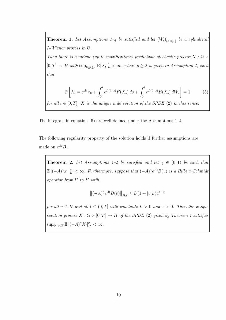
Theorem 1. Let Assumptions 1–4 be satisfied and let (Wt)t∈[0,T ] be a cylindrical
I-Wiener process in U .
Then there is a unique (up to modifications) predictable stochastic process X : Ω ×
[0, T ] → H with sup0≤t≤T E|Xt|pH < ∞, where p ≥ 2 is given in Assumption 4, such
that
P
[
Xt = eAtx0 +
∫ t
0
eA(t−s)F (Xs) ds +
∫ t
0
eA(t−s)B(Xs) dWs
]
= 1 (5)
for all t ∈ [0, T ]. X is the unique mild solution of the SPDE (2) in this sense.
The integrals in equation (5) are well defined under the Assumptions 1–4.
The following regularity property of the solution holds if further assumptions are
made on eAtB.
Theorem 2. Let Assumptions 1–4 be satisfied and let γ ∈ (0, 1) be such that
E |(−A)γx0|p
H < ∞. Furthermore, suppose that (−A)γeAtB(v) is a Hilbert–Schmidt
operator from U to H with
∥
∥(−A)γeAtB(v)∥
∥
HS≤ L (1 + |v|H) tε−
1
2
for all v ∈ H and all t ∈ (0, T ] with constants L > 0 and ε > 0. Then the unique
solution process X : Ω × [0, T ] → H of the SPDE (2) given by Theorem 1 satisfies
sup0≤t≤T E |(−A)γXt|p
H < ∞.
10

Sketch proof of Theorem 1
Introduce the real vector space Vp of all equivalence classes of predictable stochastic
processes X : Ω × [0, T ] → H with sup0≤t≤T |Xt|Lp < ∞.
Equip this space with the norm
‖X‖µ := sup0≤t≤T
eµt |Xt|Lp
for every X ∈ Vp and some µ ∈ R.
Note that the pair(
Vp, ‖·‖µ
)
is a Banach space for any µ ∈ R.
Define the mapping Φ : Vp → Vp by
(ΦX)t := eAtu0 +
∫ t
0
eA(t−s)F (Xs)ds +
∫ t
0
eA(t−s)B(Xs)dWs
for every t ∈ [0, T ] and X ∈ Vp.
First, it needs to be shown that Φ is well defined and then that it is a contraction
with respect to ‖·‖µ for an appropriate µ ∈ R. Now
‖ΦX − ΦY ‖µ ≤K
|µ|‖X − Y ‖µ + Lp
(∫ t
0
s2ε−1e2µs ds
)
1
2
‖X − Y ‖µ
≤
K
|µ|+ Lp
√
∫ T
0
s2ε−1e2µs ds
‖X − Y ‖µ
for µ < 0.
Hence Φ is a contraction with respect to ‖·‖µ for µ ≪ 0 and it has a unique fixed point
X ∈ Vp, which is the desired solution.
11
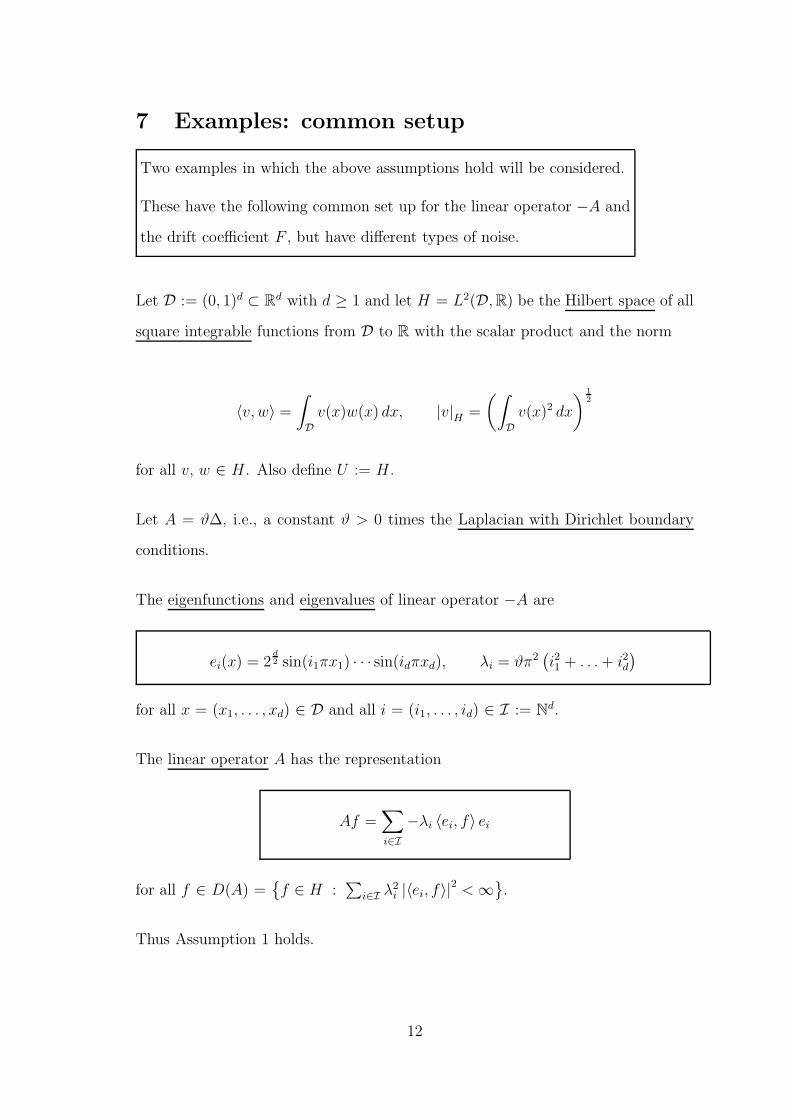
7 Examples: common setup
Two examples in which the above assumptions hold will be considered.
These have the following common set up for the linear operator −A and
the drift coefficient F , but have different types of noise.
Let D := (0, 1)d ⊂ Rd with d ≥ 1 and let H = L2(D, R) be the Hilbert space of all
square integrable functions from D to R with the scalar product and the norm
〈v, w〉 =
∫
D
v(x)w(x) dx, |v|H =
(∫
D
v(x)2 dx
)1
2
for all v, w ∈ H . Also define U := H .
Let A = ϑ∆, i.e., a constant ϑ > 0 times the Laplacian with Dirichlet boundary
conditions.
The eigenfunctions and eigenvalues of linear operator −A are
ei(x) = 2d2 sin(i1πx1) · · · sin(idπxd), λi = ϑπ2
(
i21 + . . . + i2d)
for all x = (x1, . . . , xd) ∈ D and all i = (i1, . . . , id) ∈ I := Nd.
The linear operator A has the representation
Af =∑
i∈I
−λi 〈ei, f〉 ei
for all f ∈ D(A) =
f ∈ H :∑
i∈I λ2i |〈ei, f〉|
2< ∞
.
Thus Assumption 1 holds.
12
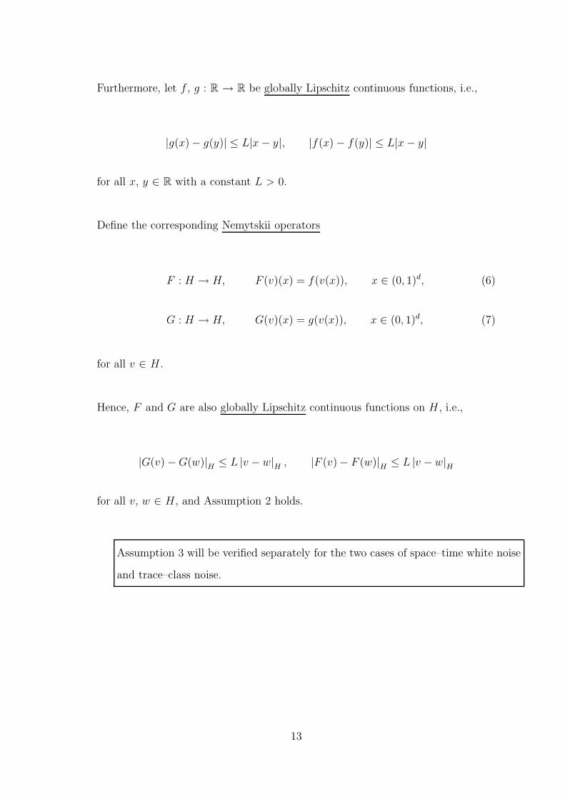
Furthermore, let f , g : R → R be globally Lipschitz continuous functions, i.e.,
|g(x) − g(y)| ≤ L|x − y|, |f(x) − f(y)| ≤ L|x − y|
for all x, y ∈ R with a constant L > 0.
Define the corresponding Nemytskii operators
F : H → H, F (v)(x) = f(v(x)), x ∈ (0, 1)d, (6)
G : H → H, G(v)(x) = g(v(x)), x ∈ (0, 1)d, (7)
for all v ∈ H .
Hence, F and G are also globally Lipschitz continuous functions on H , i.e.,
|G(v) − G(w)|H ≤ L |v − w|H , |F (v) − F (w)|H ≤ L |v − w|H
for all v, w ∈ H , and Assumption 2 holds.
Assumption 3 will be verified separately for the two cases of space–time white noise
and trace–class noise.
13
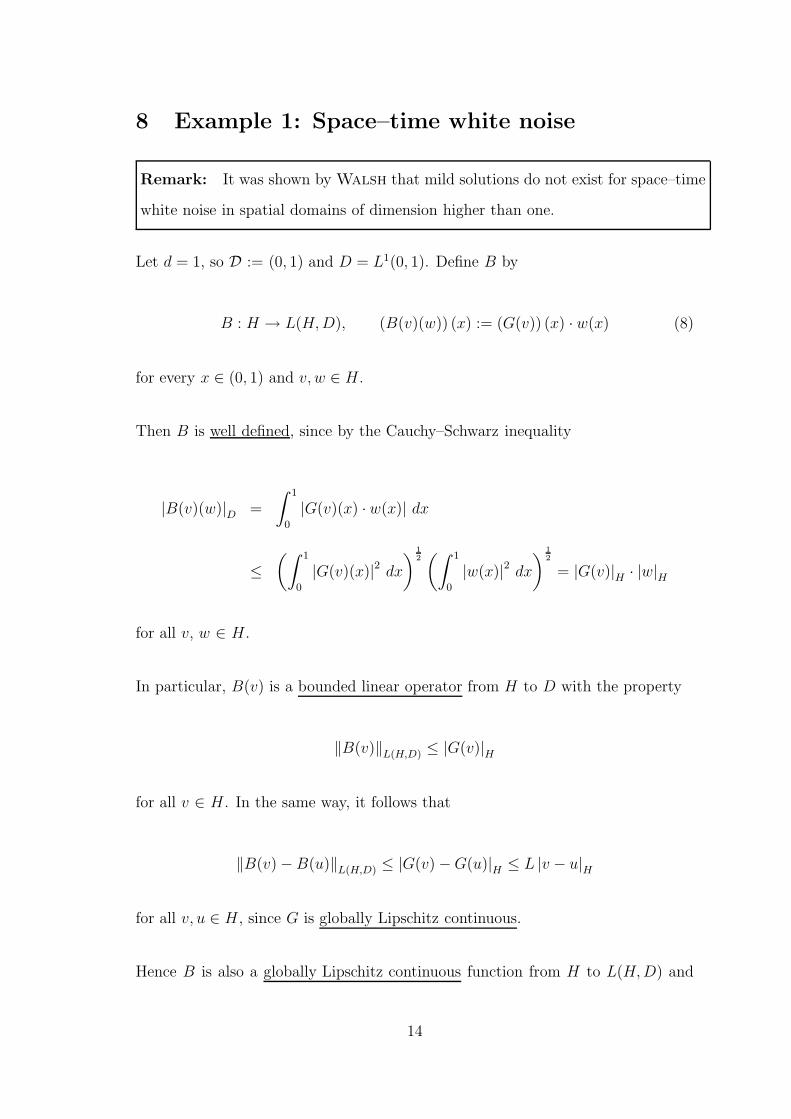
8 Example 1: Space–time white noise
Remark: It was shown by Walsh that mild solutions do not exist for space–time
white noise in spatial domains of dimension higher than one.
Let d = 1, so D := (0, 1) and D = L1(0, 1). Define B by
B : H → L(H, D), (B(v)(w)) (x) := (G(v)) (x) · w(x) (8)
for every x ∈ (0, 1) and v, w ∈ H .
Then B is well defined, since by the Cauchy–Schwarz inequality
|B(v)(w)|D =
∫ 1
0
|G(v)(x) · w(x)| dx
≤
(∫ 1
0
|G(v)(x)|2 dx
)
1
2(∫ 1
0
|w(x)|2 dx
)
1
2
= |G(v)|H · |w|H
for all v, w ∈ H .
In particular, B(v) is a bounded linear operator from H to D with the property
‖B(v)‖L(H,D) ≤ |G(v)|H
for all v ∈ H . In the same way, it follows that
‖B(v) − B(u)‖L(H,D) ≤ |G(v) − G(u)|H ≤ L |v − u|H
for all v, u ∈ H , since G is globally Lipschitz continuous.
Hence B is also a globally Lipschitz continuous function from H to L(H, D) and
14
thus measurable.
In the next step, let γ ≥ 0. Then (−A)γeAtB(v) is a bounded linear operator from
H to H for every v ∈ H and t ∈ (0, T ], since
∥
∥(−A)γeAtB(v)∥
∥
HS=
(
∑
i∈I
∑
j∈I
(
λ2γj e−2λjt |〈ej, B(v)ei〉|
2)
)1
2
≤
(
∑
j∈I
(
λ2γj e−2λj t 2 |G(v)|2H
)
)1
2
=√
2 |G(v)|H∥
∥(−A)γeAt∥
∥
HS
for all v ∈ H , t ∈ (0, T ].
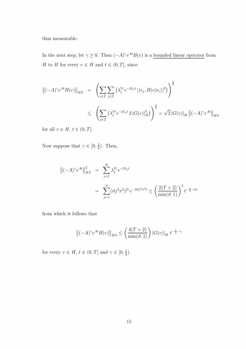
Now suppose that γ ∈ [0, 14). Then,
∥
∥(−A)γeAt∥
∥
2
HS=
∞∑
j=1
λ2γj e−2λjt
=
∞∑
j=1
(ϑj2π2)2γe−2ϑj2π2t ≤
(
2(T + 2)
min(ϑ, 1)
)2
t−1
2−2γ
from which it follows that
∥
∥(−A)γeAtB(v)∥
∥
HS≤
(
4(T + 2)
min(ϑ, 1)
)
|G(v)|H t−1
4−γ
for every v ∈ H , t ∈ (0, T ] and γ ∈ [0, 14).
15
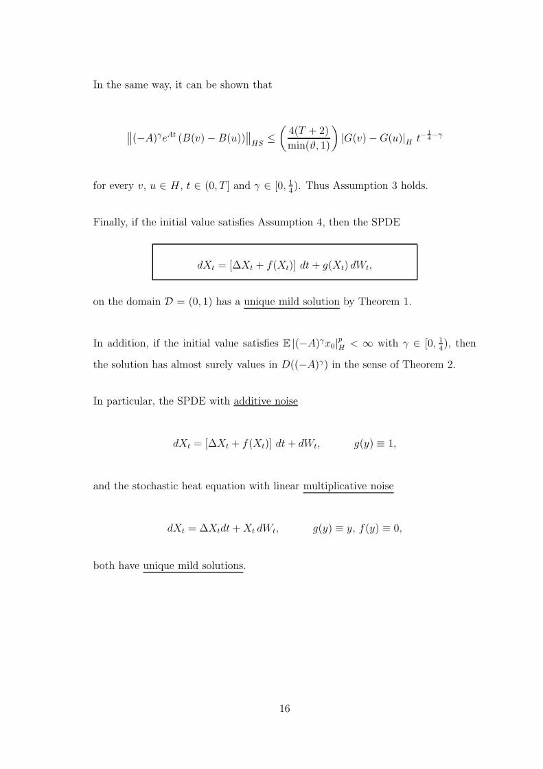
In the same way, it can be shown that
∥
∥(−A)γeAt (B(v) − B(u))∥
∥
HS≤
(
4(T + 2)
min(ϑ, 1)
)
|G(v) − G(u)|H t−1
4−γ
for every v, u ∈ H , t ∈ (0, T ] and γ ∈ [0, 14). Thus Assumption 3 holds.
Finally, if the initial value satisfies Assumption 4, then the SPDE
dXt = [∆Xt + f(Xt)] dt + g(Xt) dWt,
on the domain D = (0, 1) has a unique mild solution by Theorem 1.
In addition, if the initial value satisfies E |(−A)γx0|p
H < ∞ with γ ∈ [0, 14), then
the solution has almost surely values in D((−A)γ) in the sense of Theorem 2.
In particular, the SPDE with additive noise
dXt = [∆Xt + f(Xt)] dt + dWt, g(y) ≡ 1,
and the stochastic heat equation with linear multiplicative noise
dXt = ∆Xtdt + Xt dWt, g(y) ≡ y, f(y) ≡ 0,
both have unique mild solutions.
16
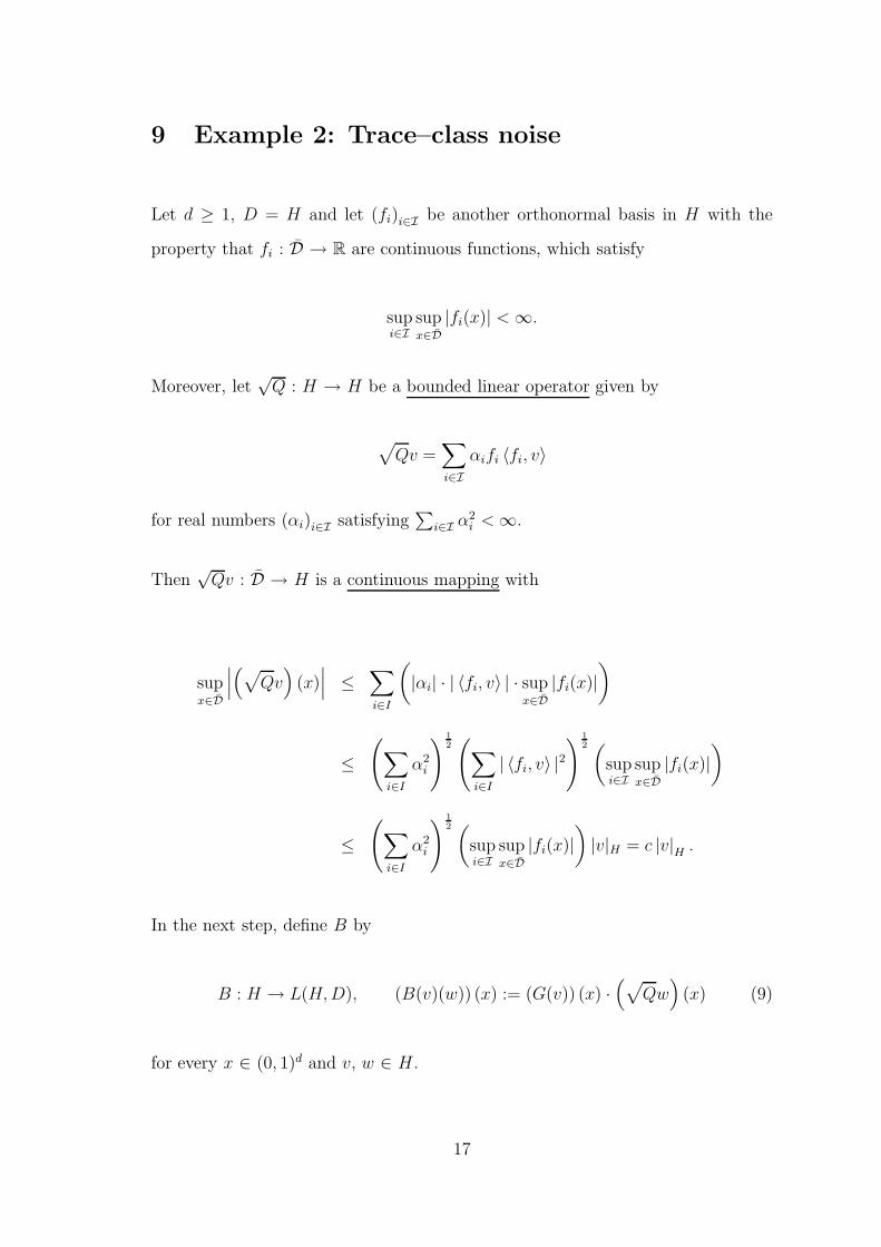
9 Example 2: Trace–class noise
Let d ≥ 1, D = H and let (fi)i∈I be another orthonormal basis in H with the
property that fi : D → R are continuous functions, which satisfy
supi∈I
supx∈D
|fi(x)| < ∞.
Moreover, let√
Q : H → H be a bounded linear operator given by
√
Qv =∑
i∈I
αifi 〈fi, v〉
for real numbers (αi)i∈I satisfying∑
i∈I α2i < ∞.
Then√
Qv : D → H is a continuous mapping with
supx∈D
∣
∣
∣
(
√
Qv)
(x)
∣
∣
∣≤
∑
i∈I
(
|αi| · | 〈fi, v〉 | · supx∈D
|fi(x)|
)
≤
(
∑
i∈I
α2i
)1
2
(
∑
i∈I
| 〈fi, v〉 |2
)1
2(
supi∈I
supx∈D
|fi(x)|
)
≤
(
∑
i∈I
α2i
)1
2(
supi∈I
supx∈D
|fi(x)|
)
|v|H = c |v|H
.
In the next step, define B by
B : H → L(H, D), (B(v)(w)) (x) := (G(v)) (x) ·(
√
Qw)
(x) (9)
for every x ∈ (0, 1)d and v, w ∈ H .
17
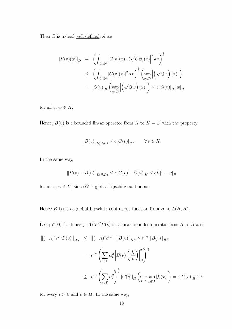
Then B is indeed well defined, since
|B(v)(w)|D =
(∫
(0,1)d
∣
∣
∣G(v)(x) · (
√
Qw)(x)∣
∣
∣
2
dx
)1
2
≤
(∫
(0,1)d
|G(v)(x)|2 dx
)1
2
(
supx∈D
∣
∣
∣
(
√
Qw)
(x)
∣
∣
∣
)
= |G(v)|H
(
supx∈D
∣
∣
∣
(
√
Qw)
(x)
∣
∣
∣
)
≤ c |G(v)|H |w|H
for all v, w ∈ H .
Hence, B(v) is a bounded linear operator from H to H = D with the property
‖B(v)‖L(H,D) ≤ c |G(v)|
H, ∀ v ∈ H.
In the same way,
‖B(v) − B(u)‖L(H,D) ≤ c |G(v) − G(u)|H ≤ cL |v − u|H
for all v, u ∈ H , since G is global Lipschitz continuous.
Hence B is also a global Lipschitz continuous function from H to L(H, H).
Let γ ∈ [0, 1). Hence (−A)γeAtB(v) is a linear bounded operator from H to H and
∥
∥(−A)γeAtB(v)∥
∥
HS≤
∥
∥(−A)γeAt∥
∥ ‖B(v)‖HS ≤ t−γ ‖B(v)‖HS
= t−γ
(
∑
i∈I
α2i
∣
∣
∣
∣
B(v)
(
fi
αi
)∣
∣
∣
∣
2
H
)1
2
≤ t−γ
(
∑
i∈I
α2i
)1
2
|G(v)|H
(
supi∈I
supx∈D
|fi(x)|
)
= c |G(v)|H t−γ
for every t > 0 and v ∈ H . In the same way,
18
∥
∥(−A)γeAt (B(v) − B(u))∥
∥
HS≤ c |G(v) − G(u)|H t−γ
for every t > 0 and v, u ∈ H , which verifies that Assumption 3.
Finally, if the initial value satisfies Assumption 4, then the SPDE
dXt = [∆Xt + f(Xt)] dt + g(Xt)√
Q dWt
on the domain D = (0, 1)d has a unique solution by Theorem 1. Moreover, if
E |(−A)γu0|p
< ∞ with γ ∈ [0, 12), then the solution has almost surely values in
D((−A)γ) in the sense of Theorem 2.
In particular, the SPDE with additive noise
dXt = [∆Xt + f(Xt)] dt +√
QdWt, g(y) ≡ 1,
and the stochastic heat equation with linear multiplicative noise
dXt = ∆Xtdt + Xt
√
Q dWt, g(y) ≡ y, f(y) ≡ 0,
both have unique mild solutions.
19
Lecture 6: Numerical Methods for SPDEs
The numerical approximation of stochastic partial differential equations
(SPDEs), specifically stochastic evolution equations of the parabolic or hy-
perbolic type, encounters all of the difficulties that arise in the numerical
solution of both deterministic PDEs and finite dimensional stochastic ordi-
nary differential equations (SODEs) as well as many more due to the infinite
dimensional nature of the driving noise process.
The state of development of numerical schemes for SPDEs compares with
that for SODEs in the early 1970s.
However, most of the numerical schemes that have been proposed to date
have a low order of convergence, especially in terms of an overall computa-
tional effort.
Only recently has it been shown how to construct higher order schemes.
1
The breakthrough for SODEs started with the Milstein scheme and contin-
ued with the systematic derivation of stochastic Taylor expansions and the
numerical schemes based on them.
These stochastic Taylor schemes are based on an iterated application of the
Ito formula.
The crucial point is that the multiple stochastic integrals which they contain
provide more information about the noise processes within discretisation
subintervals and this allows an approximation of higher order to be obtained.
There is, however, NO general Ito formula for the solutions of SPDEs in
Hilbert spaces or Banach spaces.
Nevertheless, it has recently been shown that Taylor expansions for the
solutions of such equations can be constructed by taking advantage of the
mild form representation of the solutions.
2
1 An early result
Consider a parabolic SPDE with a Dirichlet boundary condition on a bounded
domain D in Rd
dXt = [AXt + F (Xt)] dt + G(Xt) dWt. (1)
Suppose that the coefficients satisfy the assumptions of the previous lecture. In
particular, assume that the eigenvalues λj and the corresponding eigenfunctions φj
∈ H1,20 (D) of the linear operator −A , i.e., with
−Aφj = λjφj , j = 1, 2, . . . ,
form an orthonormal basis in L2(D) with λj → ∞ as j → ∞.
• Assume (for now) also that Wt is a standard scalar Wiener process.
Projecting the SPDE (1) onto the N -dimensional subspace HN of L2(D) spanned
by φ1, . . ., φN gives an N -dimensional Ito–Galerkin SODE in RN of the form
dX(N)t =
[
ANX(N)t + FN(X
(N)t )
]
dt + GN(X(N)t ) dWt, (2)
where X(N) is written synonomously for (XN,1, · · · , XN,N)⊤ ∈ RN or
∑N
j=1 XN,jφj
∈ HN according to the context.
Moreover, FN = PNF∣
∣
HNand GN = PNG
∣
∣
HN, where F and G are now interpreted
as mappings of L2(D) or H1,20 (D) into itself, and PN is the projection of L2(D) or
H1,20 (D) onto HN , while AN = PNA
∣
∣
HNis the diagonal matrix diag [λj , . . . , λN ].
3
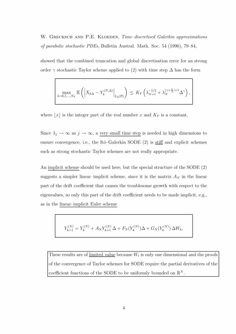
W. Grecksch and P.E. Kloeden, Time–discretised Galerkin approximations
of parabolic stochastic PDEs, Bulletin Austral. Math. Soc. 54 (1996), 79–84,
showed that the combined truncation and global discretisation error for an strong
order γ stochastic Taylor scheme applied to (2) with time step ∆ has the form
maxk=0,1,...,NT
E
(
∣
∣
∣Xk∆ − Y
(N,∆)k
∣
∣
∣
L2(D)
)
≤ KT
(
λ−1/2N+1 + λ
⌊γ+ 1
2⌋+1
N ∆γ)
,
where ⌊x⌋ is the integer part of the real number x and KT is a constant.
Since λj → ∞ as j → ∞, a very small time step is needed in high dimensions to
ensure convergence, i.e., the Ito–Galerkin SODE (2) is stiff and explicit schemes
such as strong stochastic Taylor schemes are not really appropriate.
An implicit scheme should be used here, but the special structure of the SODE (2)
suggests a simpler linear–implicit scheme, since it is the matrix AN in the linear
part of the drift coefficient that causes the troublesome growth with respect to the
eigenvalues, so only this part of the drift coefficient needs to be made implicit, e.g.,
as in the linear–implicit Euler scheme
Y(N)k+1 = Y
(N)k + ANY
(N)k+1 ∆ + FN(Y
(N)k )∆ + GN(Y
(N)k ) ∆Wk,
These results are of limited value because Wt is only one dimensional and the proofs
of the convergence of Taylor schemes for SODE require the partial derivatives of the
coefficient functions of the SODE to be uniformly bounded on RN .
4
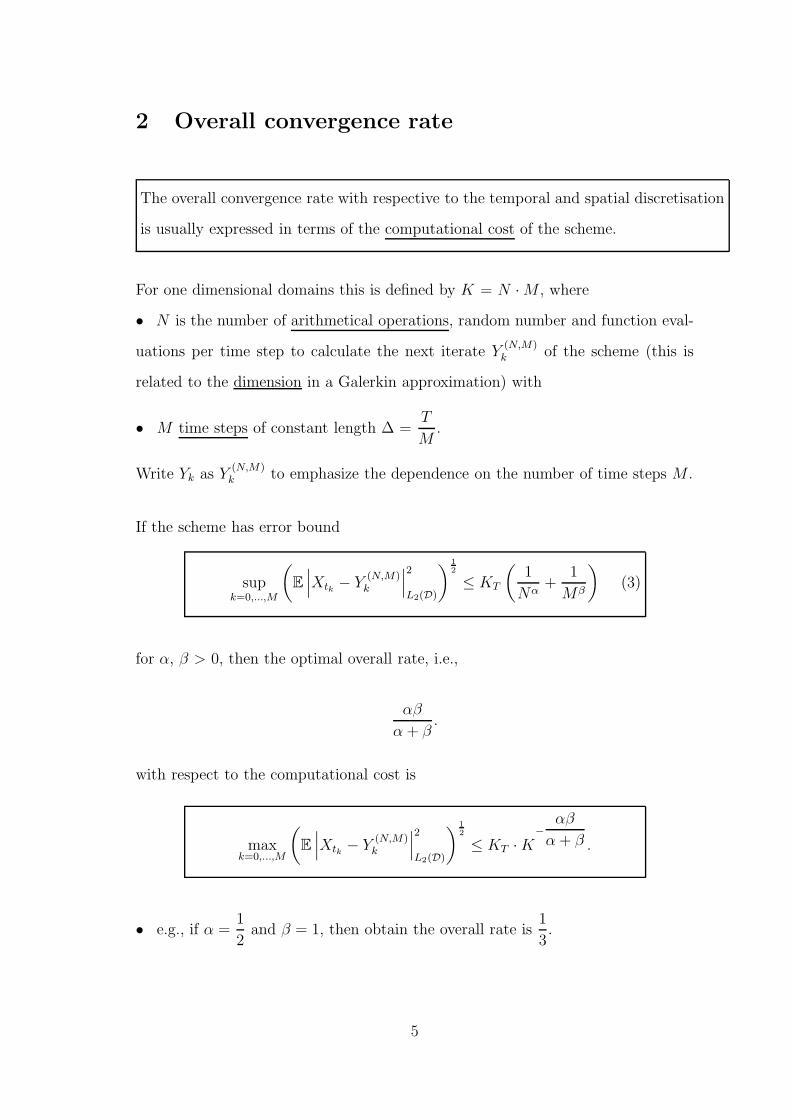
2 Overall convergence rate
The overall convergence rate with respective to the temporal and spatial discretisation
is usually expressed in terms of the computational cost of the scheme.
For one dimensional domains this is defined by K = N · M , where
• N is the number of arithmetical operations, random number and function eval-
uations per time step to calculate the next iterate Y(N,M)k of the scheme (this is
related to the dimension in a Galerkin approximation) with
• M time steps of constant length ∆ =T
M.
Write Yk as Y(N,M)k to emphasize the dependence on the number of time steps M .
If the scheme has error bound
supk=0,...,M
(
E
∣
∣
∣Xtk − Y
(N,M)k
∣
∣
∣
2
L2(D)
)1
2
≤ KT
(
1
Nα+
1
Mβ
)
(3)
for α, β > 0, then the optimal overall rate, i.e.,
αβ
α + β.
with respect to the computational cost is
maxk=0,...,M
(
E
∣
∣
∣Xtk − Y
(N,M)k
∣
∣
∣
2
L2(D)
)1
2
≤ KT · K−
αβ
α + β .
• e.g., if α =1
2and β = 1, then obtain the overall rate is
1
3.
5
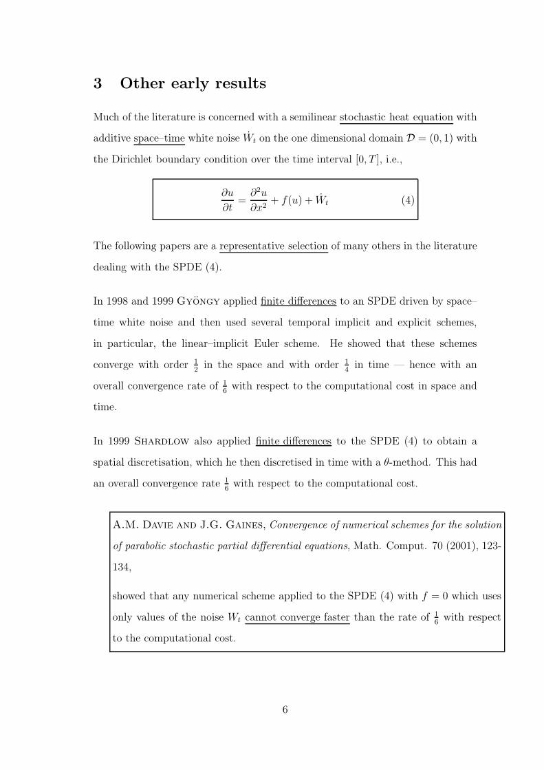
3 Other early results
Much of the literature is concerned with a semilinear stochastic heat equation with
additive space–time white noise Wt on the one dimensional domain D = (0, 1) with
the Dirichlet boundary condition over the time interval [0, T ], i.e.,
∂u
∂t=
∂2u
∂x2+ f(u) + Wt (4)
The following papers are a representative selection of many others in the literature
dealing with the SPDE (4).
In 1998 and 1999 Gyongy applied finite differences to an SPDE driven by space–
time white noise and then used several temporal implicit and explicit schemes,
in particular, the linear–implicit Euler scheme. He showed that these schemes
converge with order 12
in the space and with order 14
in time — hence with an
overall convergence rate of 16
with respect to the computational cost in space and
time.
In 1999 Shardlow also applied finite differences to the SPDE (4) to obtain a
spatial discretisation, which he then discretised in time with a θ-method. This had
an overall convergence rate 16
with respect to the computational cost.
A.M. Davie and J.G. Gaines, Convergence of numerical schemes for the solution
of parabolic stochastic partial differential equations, Math. Comput. 70 (2001), 123-
134,
showed that any numerical scheme applied to the SPDE (4) with f = 0 which uses
only values of the noise Wt cannot converge faster than the rate of 16
with respect
to the computational cost.
6
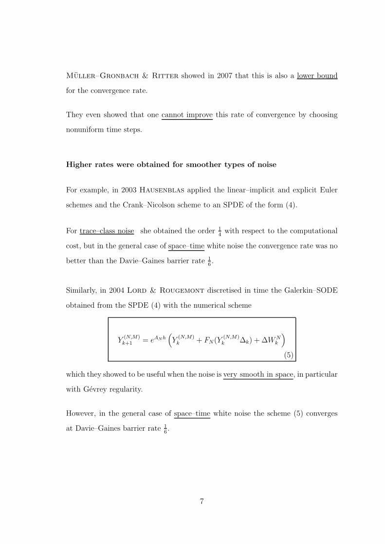
Muller–Gronbach & Ritter showed in 2007 that this is also a lower bound
for the convergence rate.
They even showed that one cannot improve this rate of convergence by choosing
nonuniform time steps.
Higher rates were obtained for smoother types of noise
For example, in 2003 Hausenblas applied the linear–implicit and explicit Euler
schemes and the Crank–Nicolson scheme to an SPDE of the form (4).
For trace–class noise she obtained the order 14
with respect to the computational
cost, but in the general case of space–time white noise the convergence rate was no
better than the Davie–Gaines barrier rate 16.
Similarly, in 2004 Lord & Rougemont discretised in time the Galerkin–SODE
obtained from the SPDE (4) with the numerical scheme
Y(N,M)k+1 = eAN h
(
Y(N,M)k + FN(Y
(N,M)k ∆k) + ∆W N
k
)
(5)
which they showed to be useful when the noise is very smooth in space, in particular
with Gevrey regularity.
However, in the general case of space–time white noise the scheme (5) converges
at Davie–Gaines barrier rate 16.
7
4 The exponential Euler scheme
A. Jentzen and P. E. Kloeden, Overcoming the order barrier in the numerical
approximation of SPDEs with additive space-time noise, Proc. Roy. Soc. London,
Series A 465 (2009), no. 2102, 649–667.
Consider a parabolic SPDE with additive noise
dXt = [AXt + F (Xt)] dt + dWt, X0 = x0, (6)
in a Hilbert space (H, | · |) with inner product < ·, · >, where A is an in general
unbounded linear operator, F : H → H is a nonlinear continuous function and Wt
is a cylindrical Wiener process.
Interpet the SPDE (6) in the mild sense
Xt = eAtx0 +
∫ t
0
eA(t−s)F (Xs) ds+
∫ t
0
eA(t−s) dWs. (7)
Use the fact that the solution of the N -dimensional Ito–Galerkin SODE in the
space HN := PNH (or, equivalently, in RN)
dXNt =
(
ANXNt + FN(XN
t ))
dt + dW Nt (8)
has an analogous “mild” representation
XNt = eAN tuN
0 +
∫ t
0
eAN (t−s)FN(XNs ) ds +
∫ t
0
eAN (t−s) dW Ns . (9)
8
This motivated what Jentzen & Kloeden called the exponential Euler scheme
Y(N,M)k+1 = eAN∆Y
(N,M)k + A−1
N
(
eAN∆ − I)
FN(Y(N,M)k )
+
∫ tk+1
tk
eAN (tk+1−s) dW Ns (10)
with the time step ∆ = TM
for some M ∈ N and discretisation times tk = k∆ for k
= 0, 1, . . . , M .
The exponential Euler scheme is easier to simulate than may seem on the first
sight.
Denoting the components of Y(N,M)k and FN by
Y(N,M)k,i =
⟨
ei, Y(N,M)k
⟩
, F iN = 〈ei, FN〉 , i = 1, . . . , N,
the numerical scheme (10) can be rewritten as
Y(N,M)k+1,1 = e−λ1∆Y
(N,M)k,1 +
(1 − e−λ1∆)
λ1F 1
N(Y(N,M)k ) +
(
q1
2λ1(1 − e−2λ1∆)
)1
2
R1k
......
...
Y(N,M)k+1,N = e−λN∆Y
(N,M)k,N +
(1 − e−λN∆)
λN
F NN (Y
(N,M)k ) +
(
qN
2λN
(1 − e−2λN∆)
)1
2
RNk ,
where the Rik for i = 1,. . . , N and k = 0, 1, . . . , M − 1 are independent, standard
normally distributed random variables.
9
5 Assumptions
Assumption 1. (Linear Operator A) There exist sequences of real eigenvalues 0
< λ1 ≤ λ2 ≤ . . . and orthonormal eigenfunctions (en)n≥1 of A such that the linear
operator A : D(A) ⊂ H → H is given by
Av =
∞∑
n=1
−λn 〈en, v〉 en
for all v ∈ D(A) with D(A) =
v ∈ H :∑∞
n=1 |λn|2 |〈en, v〉|2 < ∞
.
Assumption 2. (Nonlinearity F ) The nonlinearity F : H → H is two times
continuously Frechet differentiable and its derivatives satisfy
‖F ′(x) − F ′(y)‖ ≤ L |x − y|H ,∣
∣(−A)(−r)F ′(x)(−A)rv∣
∣
H≤ L |v|H
for all x, y ∈ H, v ∈ D((−A)r) and r = 0, 12, 1 and
∣
∣A−1F ′′(x)(v, w)∣
∣
H≤ L
∣
∣
∣(−A)−
1
2 v∣
∣
∣
H
∣
∣
∣(−A)−
1
2 w∣
∣
∣
H
for all v,w,x ∈ H, where L > 0 is a positive constant.
Assumption 3. (Cylindrical Q-Wiener process Wt) There exist a sequence (qn)n≥1
of positive real numbers and a real number γ ∈ (0, 1) such that
∞∑
n=1
λ2γ−1n qn < ∞
and pairwise independent, scalar Ft-adapted Wiener processes (W nt )t≥0 for n ≥ 1.
The cylindrical Q-Wiener process Wt is given formally by
Wt =
∞∑
n=1
√qn W n
t en.
10
Assumption 4. (Initial value) The random variable x0 : Ω → D((−A)γ)
satisfies E |(−A)γx0|4H < ∞, where γ > 0 is given in Assumption 3.
Under Assumptions 1–4 the SPDE (6) has a unique mild solution Xt on the time
interval [0, T ], where Xt is the predictable stochastic process in D((−A)γ) given by
the mild form equation (7).
Since Assumption 2 also applies to FN , the Ito–Galerkin SODE (8) also has a
unique solution on [0, T ], which is given implicitly by the mild form equation (9).
The formalism here includes space–time white noise (in one dimensional domains)
as well as trace–class noise.
Theorem 1. Suppose that Assumptions 1–4 are satisfied. Then, there is a constant
CT > 0 such that
supk=0,...,M
(
E
∣
∣
∣Xtk − Y
(N,M)k
∣
∣
∣
2
H
)1
2
≤ CT
(
λ−γ
N +log(M)
M
)
holds for all N , M ∈ N, where Xt is the solution of SPDE (6), Y(N,M)k is the
numerical solution given by (10), tk = Tk
Mfor k = 0, 1, . . . , M , and γ > 0 is the
constant given in Assumption (A2).
In fact, the exponential Euler scheme (10) converges in time with a strong order
1 − ε for an arbitrary small ε > 0 since log(M) can be estimated by Mε, so
log(M)
M≈
1
M1−ε.
An essential point is that the integral∫ tk+1
tkeAN (tk+1−s) dW N
s includes includes more
information about the noise on the discretisation interval.
11
6 Restrictiveness of the assumptions
Assumptions 1–4 in Theorem 1 are typical of those used in the mathematical lit-
erature and are interesting for when they are valid and not valid.
Assumptions 1–4 are quiet restrictive. and Theorem 1 has several
serious shortcomings.
Firstly, the eigenvalues and eigenfunctions of the operator A are rarely known
except in very simple domains — finite element methods are a possible way around
this difficulty.
More seriously, Assumption 2 on the nonlinearity F , which is understood as the
Nemytskii operator of some function f : R → R, is very restrictive and excludes
Nemytskii operators for functions like
f(u) =u
1 + u2, f(u) = u − u3, u ∈ R.
A particular problem is the Frechet differentiability of the function F when con-
sidered as a mapping on the Hilbert space H into itself and the boundedness of the
derivatives of F as expressed in Assumption 2.
The other problem is the global Lipschitz estimate on F — this difficulty also
arises for finite dimensional Ito SODE for which it can be overcome by using
pathwise convergence rather than strong convergence.
12
Lectures 7 & 8: SPDEs with Additive Noise
Taylor expansions of solutions of SPDE in Banach spaces are the basis for deriving
higher order numerical schemes for SPDE, just as for SODE.
There is, however, a major difficulty for SPDE. Although the driving Wiener process
is a martingale, the solution process is usually not even a semi–martingale.
In particular, in general, an Ito formula does not exist for the solutions of SPDEs,
just special cases.
Hence stochastic Taylor expansions for the solutions of an SPDE cannot be derived
as for the solutions of finite dimensional SODE.
In this and the next lecture we consider the derivation of robust Taylor expansions
of solutions of SPDE with additive noise of the form
dXt = [AXt + f(Xt)] dt + B dWt, (1)
which will be interpreted in mild form
Xt = Stξ +
∫ t
0
St−s F (Xs) ds + Ot
for an appropriate semigroup of operators (St)t≥0.
• The Taylor expansions will be derived in essential the same way as for RODEs.
1
1 Assumptions
Let (Ω,F , P) be a probability space and (V, |·|) be separable real Banach space.
Let (L(V ), ‖·‖) denote the real Banach space of all bounded linear operator from V
to V and let(
L(n)(V, V ), ‖·‖)
with n ∈ N be the real Banach space of all bounded
n-multilinear operators from V n to V .
Finally, let B(V ) be the Borel σ-algebra on V and fix T > 0.
A mapping Y : [0, T ] × Ω → V is said to be a stochastic process if the mappings
Yt : Ω → V, ω 7→ Yt(ω) := Y (t, ω), ω ∈ Ω,
are F/B(V )-measurable for every t ∈ [0, T ].
Such a stochastic process Y : [0, T ]×Ω → V is said to have continuous sample paths
if the mappings
[0, T ] → V, t 7→ Yt(ω), t ∈ [0, T ],
are continuous for every ω ∈ Ω.
It is said to have θ-Holder continuous sample paths where θ ∈ (0, 1] if
sup0≤t1<t2≤T
|Yt2(ω) − Yt1(ω)|
(t1 − t2)θ
< ∞
holds for every ω ∈ Ω.
2
Assumption 1 (Semigroup S). The mapping S : [0,∞) → L(V ) satisfies
S0 = I, St1St2 = St1+t2 ,
sup0≤t≤T
‖St‖ < ∞, sup0≤s<t≤T
‖St − Ss‖ · s
t − s< ∞ (2)
for every t1, t2 ∈ [0,∞), where I is the identity operator on V .
Comments on Assumption 1:
For greater generality the semigroup S : [0,∞) → L(V ) in Assumption 1 is not
assumed to be strongly continuous as is usual in the literature.
The last condition in (2) implies that St is locally Lipschitz continuous on (0, T ]
and also indicates the size of the local Lipschitz constant.
If St = eAt, t ≥ 0, is a strongly continuous semigroup on V with the generator A :
D(A) ⊂ V → V , then the last condition in (2) follows from the estimate
∥
∥AeAt∥
∥ ≤ c/t, t ∈ (0, T ],
and some constant c > 0, since
∣
∣eAt2v − eAt1v∣
∣ =∣
∣
(
eA(t2−t1) − I)
eAt1v∣
∣ =
∣
∣
∣
∣
∫ t2−t1
0
(
eAsAeAt1v)
ds
∣
∣
∣
∣
≤
∫ t2−t1
0
∣
∣eAsAeAt1v∣
∣ ds ≤
(
sup0≤t≤T
∥
∥eAt∥
∥
)
c
t1(t2 − t1) |v|
for every 0 < t1 ≤ t2 ≤ T and every v ∈ V .
3
Assumption 2 (Nonlinearity F ). The mapping F : V → V is infinitely often
Frechet differentiable.
Comments on Assumption 2: The smoothness of the drift coefficient provided
by Assumption 2 is required for the Taylor expansions that will be derived below.
The infinitely often differentiablility is assumed only for convenience and it would
suffice to assume that F is k-times Frechet differentiable for some k ∈ N, which is
sufficiently large.
Assumption 3 (Stochastic process O). The stochastic process O : [0, T ] × Ω → V
is θ-Holder continuous sample paths with θ ∈ (0, 1).
Comments on Assumption 3: This means that the mappings
Ot : Ω → V, ω 7→ Ot(ω) := O(t, ω), ω ∈ Ω,
are F/B(V )-measurable for every t ∈ [0, T ] and that
supt1,t2∈[0,T ]
t1 6=t2
|Ot2(ω) − Ot1(ω)|
|t2 − t1|θ
< ∞
holds for every ω ∈ Ω.
Pathwise Holder continuity is typical of noise processes in applications.
Assumption 3 does not require the noise process to be generated by a Wiener process
— fractional Brownian motion is also possible.
4
Assumption 4 (Initial value ξ). The initial value ξ : Ω → V is F/B(V )-measurable
with
supt∈(0,T ]
1
t|Stξ(ω) − ξ(ω)| < ∞
for every ω ∈ Ω.
Comments on Assumption 4: The condition in Assumption 4 states that the
initial random variable ξ : Ω → V is smooth in some sense. This may not be
satisfied in some applications, but can be overcome in some cases.
Assumption 5 (Existence of a solution). There exists a stochastic process X :
[0, T ] × Ω → V with continuous sample paths, which satisfies the integral equation
Xt(ω) = Stξ(ω) +
∫ t
0
St−s F (Xs(ω)) ds + Ot(ω) (3)
for every t ∈ [0, T ] and every ω ∈ Ω.
(The integral in (3) is a V -valued Bochner integral).
Comments on Assumption 5: The existence of a solution of the SPDE provided
by Assumption 5 is a minimal assumption to do numerical analysis.
It is provided by more specific assumptions on the linear operator A in the SPDE.
The explicit use of the semigroup allows greater generality and simpler notation.
5
2 Properties of the solutions
The pathwise uniqueness and Holder continuity of the solution process, the exis-
tence of which is provided by Assumption 5, follow from Assumptions 1–4.
Lemma 1. Suppose that Assumptions 1–5 are satisfied and let X, Y : Ω× [0, T ] →
V be two stochastic processes with continuous sample paths, which satisfy (3), i.e.,
Xt(ω) = Stξ(ω) +
∫ t
0
St−s F (Xs(ω)) ds + Ot(ω)
Yt(ω) = Stξ(ω) +
∫ t
0
St−s F (Ys(ω)) ds + Ot(ω)
for all t ∈ [0, T ] and ω ∈ Ω. Then
Xt(ω) = Yt(ω)
for all t ∈ [0, T ] and ω ∈ Ω.
The sample paths of the unique solution process are not only continuous, but in
fact Holder continuous.
Lemma 2. Suppose that Assumptions 1–5 hold. Then the unique solution process
X : [0, T ] × Ω → V has θ-Holder continuous sample paths, i.e.,
sup0≤t1<t2≤T
|Xt2(ω) − Xt1(ω)|
(t2 − t1)θ
< ∞
holds for every ω ∈ Ω, where θ ∈ (0, 1) is given in Assumption 3.
6
Subtracting the noise process Ot from the solution process Xt in integral equation
(3) gives the equation
Xt − Ot = Stξ +
∫ t
0
St−s F (Xs) ds (4)
for every t ∈ [0, T ].
Proposition 1. Suppose that Assumptions 1 and 2 are sastisfied and let X : [0, T ]×
Ω → V be a stochastic process with continuous sample paths. Then Y : [0, T ] × Ω
→ V given by
Yt(ω) :=
∫ t
0
St−s F (Xs(ω)) ds
for every t ∈ [0, T ] and ω ∈ Ω is a well defined stochastic process with continuous
sample paths.
The process Xt − Ot is smoother than the original solution process Xt. This
additional regularity of the stochastic process Xt − Ot will play an important role
in the derivation Taylor expansions.
Lemma 3. Suppose that Assumptions 1–5 hold. Then the stochastic process X −O
: [0, T ] × Ω → V has Lipschitz continuous sample paths, i.e.,
sup0≤t1<t2≤T
|(Xt2(ω) − Ot2(ω)) − (Xt1(ω) − Ot1(ω))|
t2 − t1< ∞
holds for every ω ∈ Ω, where O and X are given in Assumptions 3 and 5.
7
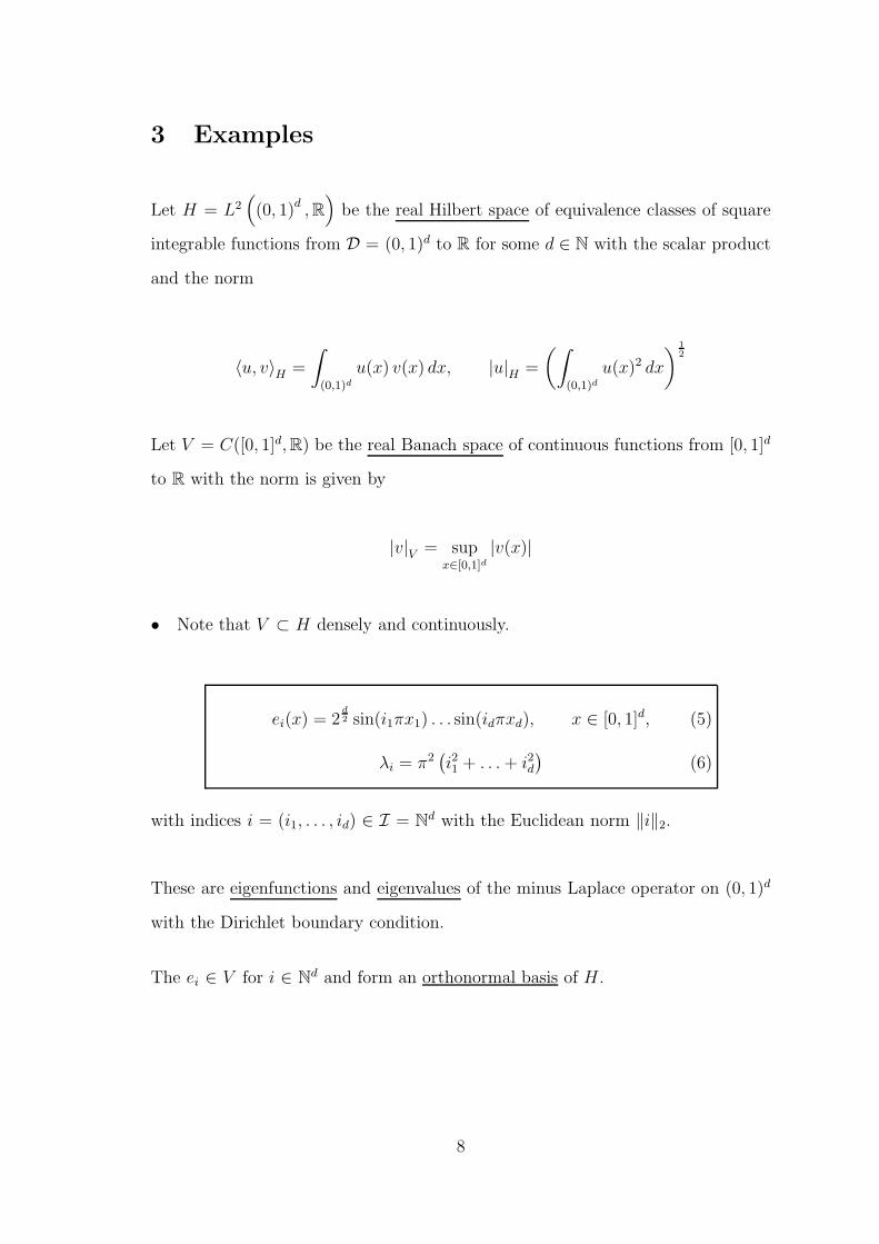
3 Examples
Let H = L2(
(0, 1)d, R)
be the real Hilbert space of equivalence classes of square
integrable functions from D = (0, 1)d to R for some d ∈ N with the scalar product
and the norm
〈u, v〉H =
∫
(0,1)d
u(x) v(x) dx, |u|H =
(∫
(0,1)d
u(x)2 dx
)1
2
Let V = C([0, 1]d, R) be the real Banach space of continuous functions from [0, 1]d
to R with the norm is given by
|v|V = supx∈[0,1]d
|v(x)|
• Note that V ⊂ H densely and continuously.
ei(x) = 2d2 sin(i1πx1) . . . sin(idπxd), x ∈ [0, 1]d, (5)
λi = π2(
i21 + . . . + i2d)
(6)
with indices i = (i1, . . . , id) ∈ I = Nd with the Euclidean norm ‖i‖2.
These are eigenfunctions and eigenvalues of the minus Laplace operator on (0, 1)d
with the Dirichlet boundary condition.
The ei ∈ V for i ∈ Nd and form an orthonormal basis of H .
8
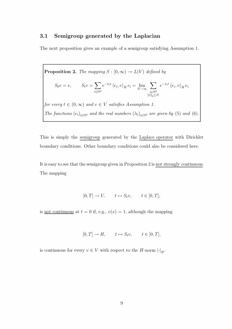
3.1 Semigroup generated by the Laplacian
The next proposition gives an example of a semigroup satisfying Assumption 1.
Proposition 2. The mapping S : [0,∞) → L(V ) defined by
S0v = v, Stv =∑
i∈Nd
e−λit 〈ei, v〉H ei = limN→∞
∑
i∈Nd
‖i‖2≤N
e−λit 〈ei, v〉H ei
for every t ∈ (0,∞) and v ∈ V satisfies Assumption 1.
The functions (ei)i∈Nd and the real numbers (λi)i∈Nd are given by (5) and (6).
This is simply the semigroup generated by the Laplace operator with Dirichlet
boundary conditions. Other boundary conditions could also be considered here.
It is easy to see that the semigroup given in Proposition 2 is not strongly continuous.
The mapping
[0, T ] → V, t 7→ Stv, t ∈ [0, T ],
is not continuous at t = 0 if, e.g., v(x) = 1, although the mapping
[0, T ] → H, t 7→ Stv, t ∈ [0, T ],
is continuous for every v ∈ V with respect to the H-norm |·|H .
9

3.2 The drift as a Nemytskii operator
The drift mapping F : V → V can often be defined as the Nemytskii operator of
a real valued function of real variables.
Let f : [0, 1]d × R → R be a continuous function such that the mappings
R → R, y 7→ f(x, y), y ∈ R, (7)
are infinitely often differentiable for each x ∈ [0, 1]d and let
∂n
∂ynf : [0, 1]d × R → R
be the nth derivative of f with respect to its last variable in [0, 1]d × R ⊂ Rd+1.
Proposition 3. Let f : [0, 1]d × R → R be a continuous function which is smooth
in its last variable in the sense of (7) such that that the partial derivatives∂n
∂ynf :
[0, 1]d × R → R are continuous for every n ∈ N.
Then the corresponding Nemytskii operator
F : V → V, (F (v)) (x) := f(x, v(x)), x ∈ [0, 1]d, v ∈ V,
is infinitely often Frechet differentiable and its Frechet derivatives F (n) : V →
L(n)(V, V ) are given by
(
F (n)(v)(v1, . . . , vn))
(x) =
(
∂n
∂ynf
)
(x, v(x)) · v1(x) · . . . · vn(x)
for every x ∈ [0, 1]d and v, v1, . . . , vn ∈ V for each n ∈ N.
Moreover, these derivatives satisfy
∥
∥F (n)(v)∥
∥ = supx∈[0,1]d
∣
∣
∣
∣
(
∂n
∂ynf
)
(x, v(x))
∣
∣
∣
∣
for every v ∈ V and n ∈ N.
10
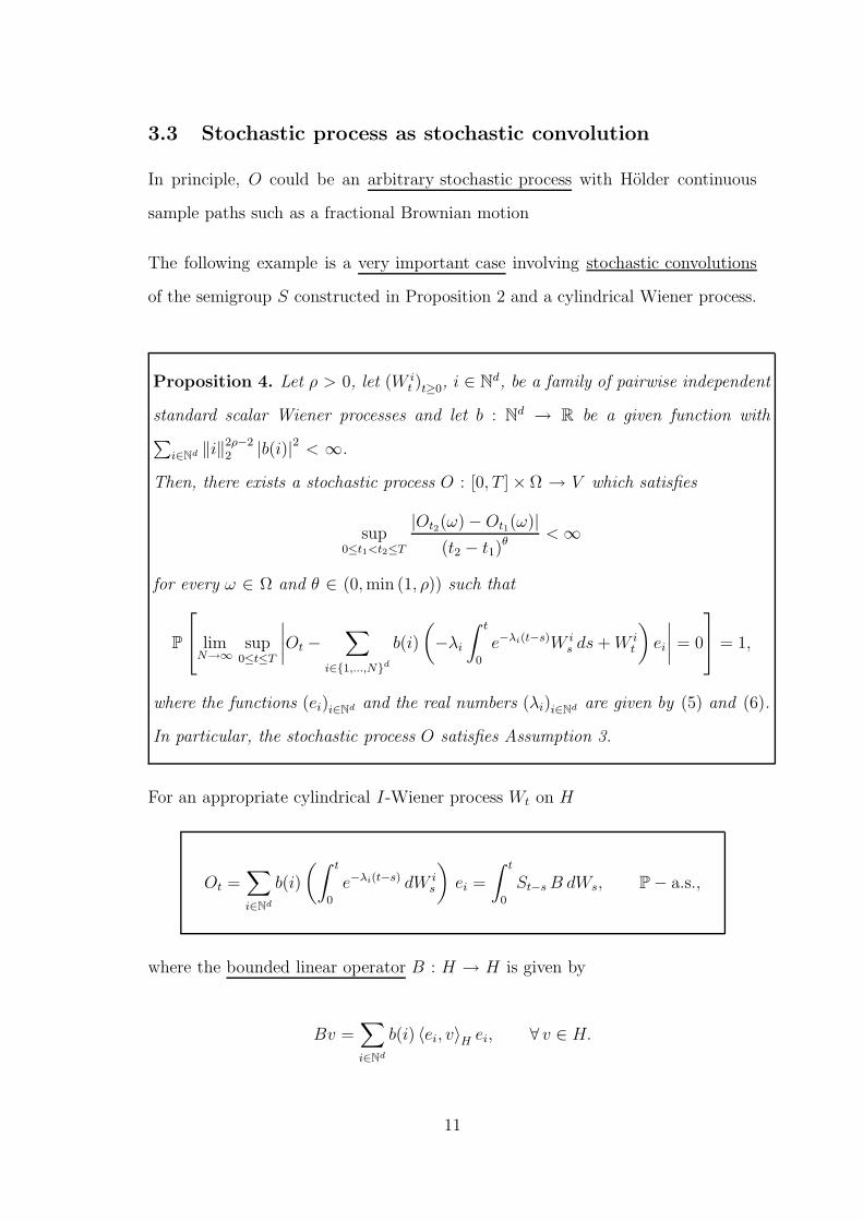
3.3 Stochastic process as stochastic convolution
In principle, O could be an arbitrary stochastic process with Holder continuous
sample paths such as a fractional Brownian motion
The following example is a very important case involving stochastic convolutions
of the semigroup S constructed in Proposition 2 and a cylindrical Wiener process.
Proposition 4. Let ρ > 0, let (W it )t≥0, i ∈ N
d, be a family of pairwise independent
standard scalar Wiener processes and let b : Nd → R be a given function with
∑
i∈Nd ‖i‖2ρ−22 |b(i)|2 < ∞.
Then, there exists a stochastic process O : [0, T ] × Ω → V which satisfies
sup0≤t1<t2≤T
|Ot2(ω) − Ot1(ω)|
(t2 − t1)θ
< ∞
for every ω ∈ Ω and θ ∈ (0, min (1, ρ)) such that
P
limN→∞
sup0≤t≤T
∣
∣
∣
∣
Ot −∑
i∈1,...,Nd
b(i)
(
−λi
∫ t
0
e−λi(t−s)W is ds + W i
t
)
ei
∣
∣
∣
∣
= 0
= 1,
where the functions (ei)i∈Nd and the real numbers (λi)i∈Nd are given by (5) and (6).
In particular, the stochastic process O satisfies Assumption 3.
For an appropriate cylindrical I-Wiener process Wt on H
Ot =∑
i∈Nd
b(i)
(∫ t
0
e−λi(t−s) dW is
)
ei =
∫ t
0
St−s B dWs, P − a.s.,
where the bounded linear operator B : H → H is given by
Bv =∑
i∈Nd
b(i) 〈ei, v〉H ei, ∀ v ∈ H.
11
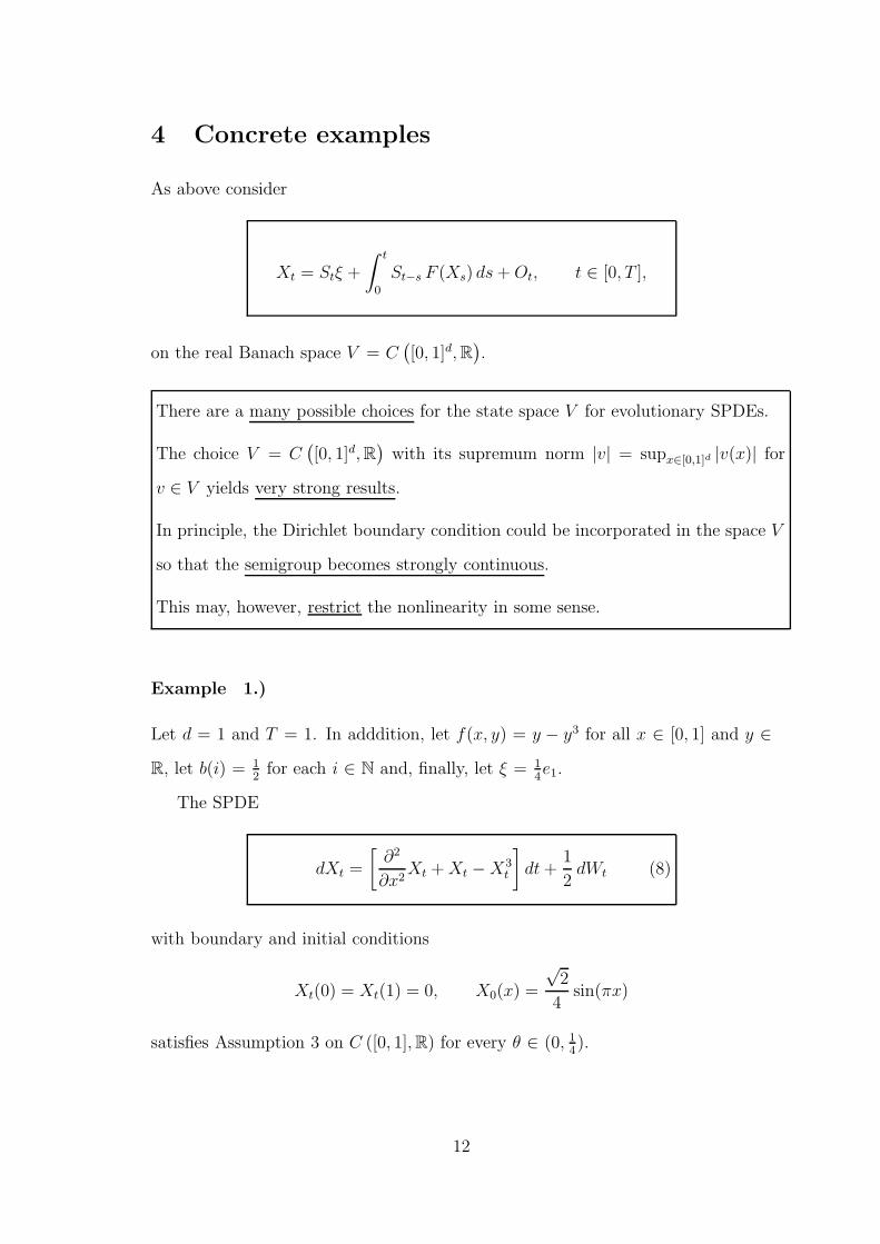
4 Concrete examples
As above consider
Xt = Stξ +
∫ t
0
St−s F (Xs) ds + Ot, t ∈ [0, T ],
on the real Banach space V = C(
[0, 1]d, R)
.
There are a many possible choices for the state space V for evolutionary SPDEs.
The choice V = C(
[0, 1]d, R)
with its supremum norm |v| = supx∈[0,1]d |v(x)| for
v ∈ V yields very strong results.
In principle, the Dirichlet boundary condition could be incorporated in the space V
so that the semigroup becomes strongly continuous.
This may, however, restrict the nonlinearity in some sense.
Example 1.)
Let d = 1 and T = 1. In adddition, let f(x, y) = y − y3 for all x ∈ [0, 1] and y ∈
R, let b(i) = 12
for each i ∈ N and, finally, let ξ = 14e1.
The SPDE
dXt =
[
∂2
∂x2Xt + Xt − X3
t
]
dt +1
2dWt (8)
with boundary and initial conditions
Xt(0) = Xt(1) = 0, X0(x) =
√2
4sin(πx)
satisfies Assumption 3 on C ([0, 1], R) for every θ ∈ (0, 14).
12
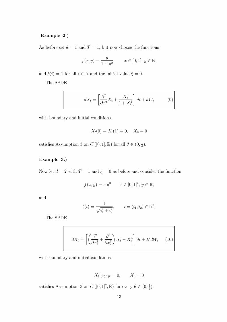
Example 2.)
As before set d = 1 and T = 1, but now choose the functions
f(x, y) =y
1 + y2, x ∈ [0, 1], y ∈ R,
and b(i) = 1 for all i ∈ N and the initial value ξ = 0.
The SPDE
dXt =
[
∂2
∂x2Xt +
Xt
1 + X2t
]
dt + dWt (9)
with boundary and initial conditions
Xt(0) = Xt(1) = 0, X0 = 0
satisfies Assumption 3 on C ([0, 1], R) for all θ ∈ (0, 14).
Example 3.)
Now let d = 2 with T = 1 and ξ = 0 as before and consider the function
f(x, y) = −y3 x ∈ [0, 1]2, y ∈ R,
and
b(i) =1
√
i21 + i22, i = (i1, i2) ∈ N
2.
The SPDE
dXt =
[(
∂2
∂x21
+∂2
∂x22
)
Xt − X3t
]
dt + B dWt (10)
with boundary and initial conditions
Xt|∂(0,1)2 = 0, X0 = 0
satisfies Assumption 3 on C ([0, 1]2, R) for every θ ∈ (0, 12).
13

5 Taylor Expansions
Recall that we are considering the pathwise SPDE with additive noise in mild form
Xt(ω) = Stξ(ω) +
∫ t
0
St−s F (Xs(ω)) ds + Ot(ω)
Taylor expansions of the solution of the SPDE (3) will be derived here in much the
same way as was done for RODEs,
i.e., using Taylor expansions of the drift function and inserting lower order Taylor
expansions of the right hand side of higher order ones to obtain a closed form
expression for the solution.
This will involve special integral operators acting on a space C of all stochastic
processes Y : [t0, T ] × Ω → V with continuous sample paths defined by
C :=
Y : [t0, T ] × Ω → V∣
∣ Yt : Ω → V is F/B(V )-measurable ∀t ∈ [t0, T ]
and [t0, T ] ∋ t 7→ Yt(ω) is continuous ∀ ω ∈ Ω
.
This is a real vector space since V is assumed to be separable.
14
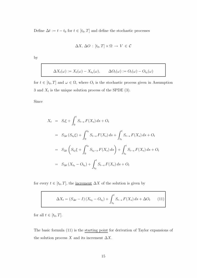
Define ∆t := t − t0 for t ∈ [t0, T ] and define the stochastic processes
∆X, ∆O : [t0, T ] × Ω → V ∈ C
by
∆Xt(ω) := Xt(ω) − Xt0(ω), ∆Ot(ω) := Ot(ω) − Ot0(ω)
for t ∈ [t0, T ] and ω ∈ Ω, where Ot is the stochastic process given in Assumption
3 and Xt is the unique solution process of the SPDE (3).
Since
Xt = Stξ +
∫ t
0
St−s F (Xs) ds + Ot
= S∆t (St0ξ) +
∫ t0
0
St−s F (Xs) ds +
∫ t
t0
St−s F (Xs) ds + Ot
= S∆t
(
St0ξ +
∫ t0
0
St0−s F (Xs) ds
)
+
∫ t
t0
St−s F (Xs) ds + Ot
= S∆t (Xt0 − Ot0) +
∫ t
t0
St−s F (Xs) ds + Ot
for every t ∈ [t0, T ], the increment ∆X of the solution is given by
∆Xt = (S∆t − I) (Xt0 − Ot0) +
∫ t
t0
St−s F (Xs) ds + ∆Ot (11)
for all t ∈ [t0, T ].
The basic formula (11) is the starting point for derivation of Taylor expansions of
the solution process X and its increment ∆X.
15

6 Integral operators
Define the stochastic processes I0 and I0∗ ∈ C by
I0(t, ω) := (S∆t − I) (Xt0(ω) − Ot0(ω)) +
(∫ ∆t
0
Ss ds
)
F (Xt0(ω))
I0∗ (t, ω) := (S∆t − I) (Xt0(ω) − Ot0(ω)) +
∫ t
t0
St−s F (Xs(ω)) ds
for every t ∈ [t0, T ] and ω ∈ Ω.
Note that the subscript ∗ means that the solution process X is included
in the integrand.
The absence of this subscript means that only the constant value Xt0 is present.
For each n ∈ N define n-multilinear symmetric mappings In and In∗ : Cn → C by
In[g1, . . . , gn](t, ω) :=1
n!
∫ t
t0
St−s F (n)(Xt0(ω)) (g1(s, ω), . . . , gn(s, ω)) ds
and
In∗ [g1, . . . , gn](t, ω) :=
∫ t
t0
St−s
(∫ 1
0
F (n)(Xt0(ω) + r∆Xs(ω)) (g1(s, ω), . . . , gn(s, ω))(1 − r)n−1
(n − 1)!dr
)
ds
for every t ∈ [t0, T ], ω ∈ Ω and g1, . . . , gn ∈ C.
It follows as in Proposition 1 from Assumptions 1–5 that the stochastic processes
I0, I0∗ ∈ C and the mappings In, In
∗ : Cn → C for n ∈ N are well defined.
16
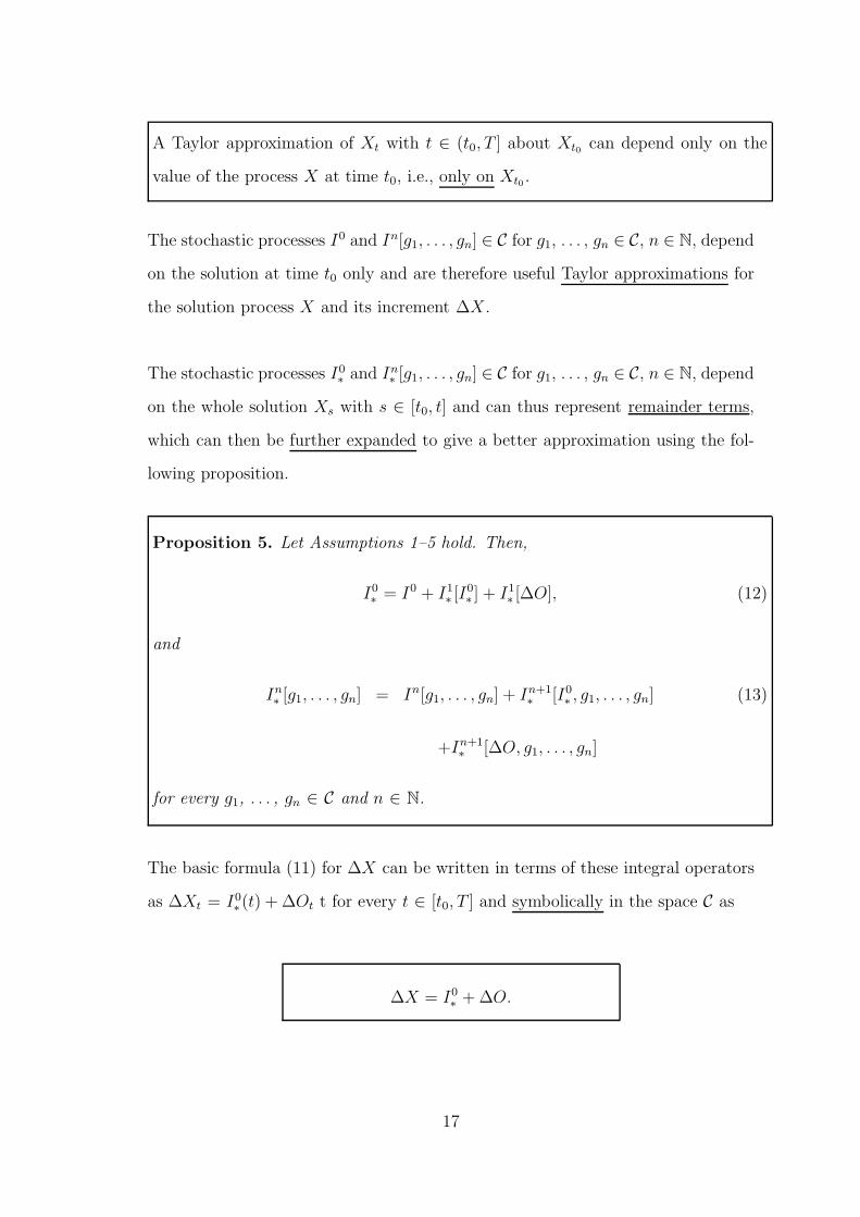
A Taylor approximation of Xt with t ∈ (t0, T ] about Xt0 can depend only on the
value of the process X at time t0, i.e., only on Xt0 .
The stochastic processes I0 and In[g1, . . . , gn] ∈ C for g1, . . . , gn ∈ C, n ∈ N, depend
on the solution at time t0 only and are therefore useful Taylor approximations for
the solution process X and its increment ∆X.
The stochastic processes I0∗ and In
∗ [g1, . . . , gn] ∈ C for g1, . . . , gn ∈ C, n ∈ N, depend
on the whole solution Xs with s ∈ [t0, t] and can thus represent remainder terms,
which can then be further expanded to give a better approximation using the fol-
lowing proposition.
Proposition 5. Let Assumptions 1–5 hold. Then,
I0∗ = I0 + I1
∗ [I0∗ ] + I1
∗ [∆O], (12)
and
In∗ [g1, . . . , gn] = In[g1, . . . , gn] + In+1
∗ [I0∗ , g1, . . . , gn] (13)
+In+1∗ [∆O, g1, . . . , gn]
for every g1, . . . , gn ∈ C and n ∈ N.
The basic formula (11) for ∆X can be written in terms of these integral operators
as ∆Xt = I0∗ (t) + ∆Ot t for every t ∈ [t0, T ] and symbolically in the space C as
∆X = I0∗ + ∆O.
17
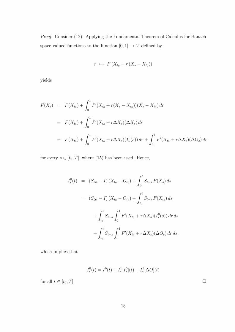
Proof. Consider (12). Applying the Fundamental Theorem of Calculus for Banach
space valued functions to the function [0, 1] → V defined by
r 7→ F (Xt0 + r (Xs − Xt0))
yields
F (Xs) = F (Xt0) +
∫ 1
0
F ′(Xt0 + r(Xs − Xt0))(Xs − Xt0) dr
= F (Xt0) +
∫ 1
0
F ′(Xt0 + r∆Xs)(∆Xs) dr
= F (Xt0) +
∫ 1
0
F ′(Xt0 + r∆Xs)(I0∗ (s)) dr +
∫ 1
0
F ′(Xt0 + r∆Xs)(∆Os) dr
for every s ∈ [t0, T ], where (15) has been used. Hence,
I0∗ (t) = (S∆t − I) (Xt0 − Ot0) +
∫ t
t0
St−s F (Xs) ds
= (S∆t − I) (Xt0 − Ot0) +
∫ t
t0
St−s F (Xt0) ds
+
∫ t
t0
St−s
∫ 1
0
F ′(Xt0 + r∆Xs)(I0∗ (s)) dr ds
+
∫ t
t0
St−s
∫ 1
0
F ′(Xt0 + r∆Xs)(∆Os) dr ds,
which implies that
I0∗ (t) = I0(t) + I1
∗ [I0∗ ](t) + I1
∗ [∆O](t)
for all t ∈ [t0, T ].
18
An iterated application of Proposition 5 then allows Taylor expansions to be de-
rived step by step, as will be seen below.
The corresponding Taylor approximation is obtained by omitting the remainder
terms in the Taylor expansion.
Write Yt = O((∆t)r) for a stochastic process Y ∈ C and some real number r
∈ (0,∞) to denote that
supt∈(t0,T ]
|Yt(ω)|
(t − t0)r< ∞
holds for every ω ∈ Ω.
The following proposition will allow the order of a Taylor approximation to be es-
timated.
Proposition 6. Let Assumptions 1–5 hold. Then I0(t) = O (∆t) and I0∗ (t) = O (∆t) .
Moreover, if g1, . . . , gn ∈ C for n ∈ N satisfy g1(t) = O ((∆t)α1), . . ., gn(t) = O ((∆t)
αn)
with α1, . . . , αn ∈ (0,∞), then
In[g1, . . . , gn](t) = O(
(∆t)1+α1+...+αn
)
, In∗ [g1, . . . , gn](t) = O
(
(∆t)1+α1+...+αn
)
. (14)
Proof. Define the F/B([0,∞))-measurable mapping R : Ω → [0,∞) by
R(ω) := 1 + sup0≤t≤T
|F (Xt(ω))| + sup0≤t≤T
‖St‖
+ sup0≤t1<t2≤T
|(Xt2(ω) − Ot2(ω)) − (Xt1(ω) − Ot1(ω))|
t2 − t1
for every ω ∈ Ω, which is indeed finite and hence well defined by Assumptions 1–5
and Lemma 3.
19
From the previous lecture
(Xt2 − Ot2) − (Xt1 − Ot1)
= (St2 − St1) ξ +
∫ t2
0
St2−s F (Xs) ds −
∫ t1
0
St1−s F (Xs) ds
= (St2−t1 − I)
(
St1ξ +
∫ t1
0
St1−s F (Xs) ds
)
+
∫ t2
t1
St2−s F (Xs) ds
= (St2−t1 − I) (Xt1 − Ot1) +
∫ t2
t1
St2−s F (Xs) ds
for all 0 ≤ t1 < t2 ≤ T .
Hence
|(St2−t1 − I) (Xt1 − Ot1)|
=
∣
∣
∣
∣
(Xt2 − Ot2) − (Xt1 − Ot1) −
∫ t2
t1
St2−s F (Xs) ds
∣
∣
∣
∣
≤ |(Xt2 − Ot2) − (Xt1 − Ot1)| +
∣
∣
∣
∣
∫ t2
t1
St2−s F (Xs) ds
∣
∣
∣
∣
≤ R (t2 − t1) + R2 (t2 − t1) ≤ 2R2 (t2 − t1)
for all 0 ≤ t1 < t2 ≤ T .
20

It follows that
∣
∣I0(t)∣
∣ =
∣
∣
∣
∣
(St−t0 − I) (Xt0 − Ot0) +
∫ t
t0
St−s F (Xt0) ds
∣
∣
∣
∣
≤ |(St−t0 − I) (Xt0 − Ot0)| +
∣
∣
∣
∣
∫ t
t0
St−s F (Xt0) ds
∣
∣
∣
∣
≤ 2R2 (t − t0) +
∫ t
t0
‖St−s‖ |F (Xt0)| ds
≤ 2R2 (t − t0) + R2 (t − t0) ≤ 3R2 (t − t0)
and
∣
∣I0∗ (t)
∣
∣ =
∣
∣
∣
∣
(St−t0 − I) (Xt0 − Ot0) +
∫ t
t0
St−s F (Xs) ds
∣
∣
∣
∣
≤ |(St−t0 − I) (Xt0 − Ot0)| +
∣
∣
∣
∣
∫ t
t0
St−s F (Xs) ds
∣
∣
∣
∣
≤ 2R2 (t − t0) +
∫ t
t0
‖St−s‖ |F (Xs)| ds
≤ 2R2 (t − t0) + R2 (t − t0) ≤ 3R2 (t − t0)
for every t ∈ [t0, T ], which shows
I0(t) = O (∆t) and I0∗ (t) = O (∆t) .
The rest of the proof is by induction.
21
7 Abstract examples of Taylor expansions
Proposition 5 will be used here to derive various Taylor expansions of the solution
X of the SPDE (3) and Proposition 6 will be used to determine their orders of
convergence.
Taylor expansion of order 1
The simplest Taylor expansion of the increment ∆X is given by the basic formula
(15), i.e.,
∆X = I0∗ + ∆O. (15)
or ∆Xt = I0∗ (t) + ∆Ot for t ∈ [t0, T ].
If the solution X is known at time t0 only, the expression I0∗ (t) cannot be used to
determine ∆Xt = Xt − Xt0 for t ∈ (t0, T ] since it contains the unknown solution
path Xs with s ∈ [t0, t] .
Omitting I0∗ gives the approximation ∆X ≈ ∆O, which can also be written as
Xt ≈ Xt0 + Ot − Ot0 , t ∈ [t0, T ]. (16)
By Proposition 6 the remainder term I0∗ of the Taylor approximation (16) can be
estimated by I0∗ (t) = O(∆t), so
Xt = Xt0 + Ot − Ot0 + O(∆t) (17)
gives the simplest Taylor approximation of the solution process X.
22
Taylor expansion of order 1 + θ
Proposition 5 can now be used to derive a higher order expansion of the
basic formula (15).
More precisely, formula (12) is inserted to the remainder stochastic process I0∗ , i.e.,
I0∗ = I0 + I1
∗ [I0∗ ] + I1
∗ [∆O]
into the basic formula (15) to give
∆X =(
I0 + I1∗ [I
0∗ ] + I1
∗ [∆O])
+ ∆O,
which can also be written as
∆X = I0 + ∆O +(
I1∗ [I
0∗ ] + I1
∗ [∆O])
. (18)
Omitting the double integral terms I1∗ [I
0∗ ] and I1
∗ [∆O] gives the Taylor approxima-
tion
∆X ≈ I0 + ∆O, (19)
which, using the definition of the stochastic process I0, is equal to
∆Xt ≈ (S∆t − I) (Xt0 − Ot0) +
(∫ ∆t
0
Ss ds
)
F (Xt0) + ∆Ot
for t ∈ [t0, T ].
23
Hence
Xt ≈ S∆tXt0 +
(∫ ∆t
0
Ss ds
)
F (Xt0) + (Ot − S∆tOt0) (20)
is another Taylor approximation for the solution of the SPDE (3).
By Proposition 6, I0∗ (t) = O (∆t) and, by Assumption 3, ∆Ot = O
(
(∆t)θ)
. Hence
from (14) it follows that
I1∗ [I
0∗ ](t) = O
(
(∆t)2)
, I1∗ [∆O](t) = O
(
(∆t)1+θ)
.
Since 1 + θ < 2, these imply that
I1∗ [I
0∗ ](t) + I1
∗ [∆O](t) = O(
(∆t)1+θ)
.
Hence, from (18),
∆X = I0 + ∆O + O(
(∆t)1+θ)
It then follows from the definition of the stochastic process I0 ∈ C that
Xt = S∆tXt0 +
(∫ ∆t
0
Ss ds
)
F (Xt0) + (Ot − S∆tOt0) + O(
(∆t)1+θ)
. (21)
The Taylor approximation (21) plays an analogous role to the strong order γ =
0.5 Taylor expansion giving the Euler–Maruyama scheme for finite dimensional
SODEs.
It will be called the exponential Euler approximation since it gives the exponential
Euler scheme for SPDES with additive noise.
24
Taylor expansion of order 1 + min(1, 2θ)
Further expansions of the remainder terms in a Taylor expansion give a Taylor
expansion of higher order.
The remainder term of (18) consists of two terms: I1∗ [I
0∗ ] and I1
∗ [∆O].
There are now two possibilities for obtaining a higher order Taylor expansion:
expand either
I1∗ [I
0∗ ](t) = O
(
(∆t)2)
or I1∗ [∆O](t) = O
(
(∆t)1+θ)
.
Since 1 + θ < 2 by Assumption 3, the stochastic process I1∗ [∆O] is of lower order
than I1∗ [I
0∗ ].
Hence the term I1∗ [∆O] should be expanded to improve on the approximation order
1 + θ of the Taylor approximation (21).
More precisely, from (13),
I1∗ [∆O] = I1[∆O] + I2
∗ [I0∗ , ∆O] + I2
∗ [∆O, ∆O],
which is inserted into (18) to yield
∆X =(
I0 + ∆O + I1[∆O])
+ R, (22)
where the remainder term R ∈ C is given by
R = I1∗ [I
0∗ ] + I2
∗ [I0∗ , ∆O] + I2
∗ [∆O, ∆O]. (23)
25
By Proposition 6
I1∗ [I
0∗ ](t) = O
(
(∆t)2)
, I2∗ [I
0∗ , ∆O](t) = O
(
(∆t)2+θ)
,
I2∗ [∆O, ∆O](t) = O
(
(∆t)1+2θ
)
.
Since min(2, 2 + θ, 1 + 2θ) = 1 + min(1, 2θ), it follows that
R = O(
(∆t)1+min(1,2θ)
)
.
Thus
∆Xt = I0(t) + ∆Ot + I1[∆O](t) + O(
(∆t)1+min(1,2θ)
)
.
This can also be written as
Xt = S∆tXt0 +
(∫ ∆t
0
Ss ds
)
F (Xt0) + (Ot − S∆tOt0)
+
∫ t
t0
St−sF′(Xt0)∆Os ds + O
(
(∆t)1+min(1,2θ).
)
(24)
This is a Taylor approximation of order 1 + min(1, 2θ).
26
Taylor expansion of order 1 + min(1, 3θ)
The remainder term (23) consists of three parts, namely
I1∗ [I
0∗ ](t) = O
(
(∆t)2)
, I2∗ [I
0∗ , ∆O](t) = O
(
(∆t)2+θ)
,
I2∗ [∆O, ∆O](t) = O
(
(∆t)1+2θ
)
.
Let θ < 12
. Then min(2, 2+θ, 1+2θ) = 1+2θ and the stochastic process I2∗ [∆O, ∆O]
will be expanded here.
Applying Propostion 5 to this term yields
I2∗ [∆O, ∆O] = I2[∆O, ∆O] + I3
∗ [I0∗ , ∆O, ∆O] + I3
∗ [∆O, ∆O, ∆O]
and inserting this into (22) then gives
∆X = I0 + ∆O + I1[∆O] + I2[∆O, ∆O] + R
with remainder
R = I1∗ [I
0∗ ] + I2
∗ [I0∗ , ∆O] + I3
∗ [I0∗ , ∆O, ∆O] + I3
∗ [∆O, ∆O, ∆O].
Then R = O(
(∆t)1+min(1,3θ)
)
, since by Proposition 6
I3∗ [I
0∗ , ∆O, ∆O](t) = O
(
(∆t)2+2θ)
, I3∗ [∆O, ∆O, ∆O](t) = O
(
(∆t)1+3θ)
,
because here min(2, 2 + θ, 2 + 2θ, 1 + 3θ) = 1 + min(1, 3θ).
The resulting Taylor expansion is
Xt = S∆tXt0 +
(∫ ∆t
0
Ss ds
)
F (Xt0) + (Ot − S∆tOt0) +
∫ t
t0
St−sF′(Xt0)∆Os ds
+1
2
∫ t
t0
St−sF′′(Xt0) (∆Os, ∆Os) ds + O
(
(∆t)1+min(1,3θ)
)
. (25)
27
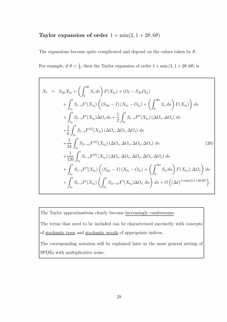
Taylor expansion of order 1 + min(2, 1 + 2θ, 6θ)
The expansions become quite complicated and depend on the values taken by θ.
For example, if θ < 14, then the Taylor expansion of order 1 + min (2, 1 + 2θ, 6θ) is
Xt = S∆tXt0 +
(∫ ∆t
0
Ss ds
)
F (Xt0) + (Ot − S∆tOt0)
+
∫ t
t0
St−sF′(Xt0)
(
(S∆s − I) (Xt0 − Ot0) +
(∫ ∆s
0
Su du
)
F (Xt0)
)
ds
+
∫ t
t0
St−sF′(Xt0)∆Os ds +
1
2
∫ t
t0
St−sF′′(Xt0) (∆Os, ∆Os) ds
+1
6
∫ t
t0
St−sF(3)(Xt0) (∆Os, ∆Os, ∆Os) ds
+1
24
∫ t
t0
S(t−s)F(4)(Xt0) (∆Os, ∆Os, ∆Os, ∆Os) ds (26)
+1
120
∫ t
t0
St−sF(5)(Xt0) (∆Os, ∆Os, ∆Os, ∆Os, ∆Os) ds
+
∫ t
t0
St−sF′′(Xt0)
(
(S∆s − I) (Xt0 − Ot0) +
(∫ ∆s
0
Su du
)
F (Xt0), ∆Os
)
ds
+
∫ t
t0
St−sF′(Xt0)
(∫ s
t0
S(s−u)F′(Xt0)∆Ou du
)
ds + O(
(∆t)1+min(2,1+2θ,6θ)
)
.
The Taylor approximations clearly become increasingly cumbersome.
The terms that need to be included can be characterised succinctly with concepts
of stochastic trees and stochastic woods of appropriate indices.
The corresponding notation will be explained later in the more general setting of
SPDEs with multiplicative noise.
28
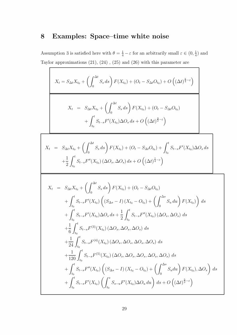
8 Examples: Space–time white noise
Assumption 3 is satisfied here with θ = 14−ε for an arbitrarily small ε ∈ (0, 1
4) and
Taylor approximations (21), (24) , (25) and (26) with this parameter are
Xt = S∆tXt0 +
(∫ ∆t
0
Ss ds
)
F (Xt0) + (Ot − S∆tOt0) + O(
(∆t)5
4−ε)
Xt = S∆tXt0 +
(∫ ∆t
0
Ss ds
)
F (Xt0) + (Ot − S∆tOt0)
+
∫ t
t0
St−sF′(Xt0)∆Os ds + O
(
(∆t)3
2−ε)
Xt = S∆tXt0 +
(∫ ∆t
0
Ss ds
)
F (Xt0) + (Ot − S∆tOt0) +
∫ t
t0
St−sF′(Xt0)∆Os ds
+1
2
∫ t
t0
St−sF′′(Xt0) (∆Os, ∆Os) ds + O
(
(∆t)7
4−ε)
Xt = S∆tXt0 +
(∫ ∆t
0
Ss ds
)
F (Xt0) + (Ot − S∆tOt0)
+
∫ t
t0
St−sF′(Xt0)
(
(S∆s − I) (Xt0 − Ot0) +
(∫ ∆s
0
Su du
)
F (Xt0)
)
ds
+
∫ t
t0
St−sF′(Xt0)∆Os ds +
1
2
∫ t
t0
St−sF′′(Xt0) (∆Os, ∆Os) ds
+1
6
∫ t
t0
St−sF(3)(Xt0) (∆Os, ∆Os, ∆Os) ds
+1
24
∫ t
t0
St−sF(4)(Xt0) (∆Os, ∆Os, ∆Os, ∆Os) ds
+1
120
∫ t
t0
St−sF(5)(Xt0) (∆Os, ∆Os, ∆Os, ∆Os, ∆Os) ds
+
∫ t
t0
St−sF′′(Xt0)
(
(S∆s − I) (Xt0 − Ot0) +
(∫ ∆s
0
Sudu
)
F (Xt0), ∆Os
)
ds
+
∫ t
t0
St−sF′(Xt0)
(∫ s
t0
Ss−uF′(Xt0)∆Ou du
)
ds + O(
(∆t)5
2−ε)
29
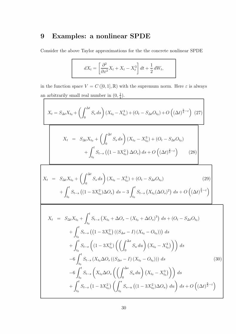
9 Examples: a nonlinear SPDE
Consider the above Taylor approximations for the the concrete nonlinear SPDE
dXt =
[
∂2
∂x2Xt + Xt − X3
t
]
dt +1
2dWt,
in the function space V = C ([0, 1], R) with the supremum norm. Here ε is always
an arbitrarily small real number in (0, 14).
Xt = S∆tXt0 +
(∫ ∆t
0
Ss ds
)
(Xt0 −X3t0
)+(Ot − S∆tOt0)+O(
(∆t)5
4−ε)
(27)
Xt = S∆tXt0 +
(∫ ∆t
0
Ss ds
)
(Xt0 − X3t0) + (Ot − S∆tOt0)
+
∫ t
t0
St−s
((
1 − 3X2t0
)
∆Os
)
ds + O(
(∆t)3
2−ε)
(28)
Xt = S∆tXt0 +
(∫ ∆t
0
Ss ds
)
(Xt0 − X3t0) + (Ot − S∆tOt0) (29)
+
∫ t
t0
St−s
(
(1 − 3X2t0)∆Os
)
ds − 3
∫ t
t0
St−s
(
Xt0(∆Os)2)
ds + O(
(∆t)7
4−ε)
Xt = S∆tXt0 +
∫ t
t0
St−s
(
Xt0 + ∆Os − (Xt0 + ∆Os)3)
ds + (Ot − S∆tOt0)
+
∫ t
t0
St−s
((
1 − 3X2t0
)
((S∆s − I) (Xt0 − Ot0)))
ds
+
∫ t
t0
St−s
(
(1 − 3X2t0)
((∫ ∆s
0
Su du
)
(
Xt0 − X3t0
)
))
ds
−6
∫ t
t0
St−s (Xt0∆Os ((S∆s − I) (Xt0 − Ot0))) ds (30)
−6
∫ t
t0
St−s
(
Xt0∆Os
((∫ ∆s
0
Su du
)
(
Xt0 − X3t0
)
))
ds
+
∫ t
t0
St−s
(
1 − 3X2t0
)
(∫ s
t0
Ss−u
(
(1 − 3X2t0)∆Ou
)
du
)
ds + O(
(∆t)5
2−ε)
30
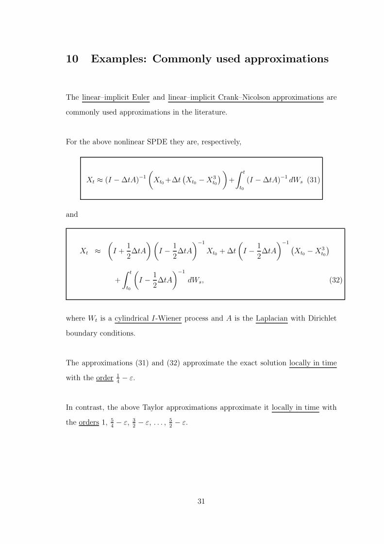
10 Examples: Commonly used approximations
The linear–implicit Euler and linear–implicit Crank–Nicolson approximations are
commonly used approximations in the literature.
For the above nonlinear SPDE they are, respectively,
Xt ≈ (I − ∆tA)−1
(
Xt0 +∆t(
Xt0 − X3t0
)
)
+
∫ t
t0
(I − ∆tA)−1
dWs (31)
and
Xt ≈
(
I +1
2∆tA
)(
I −1
2∆tA
)−1
Xt0 + ∆t
(
I −1
2∆tA
)−1(
Xt0 − X3t0
)
+
∫ t
t0
(
I −1
2∆tA
)−1
dWs, (32)
where Wt is a cylindrical I-Wiener process and A is the Laplacian with Dirichlet
boundary conditions.
The approximations (31) and (32) approximate the exact solution locally in time
with the order 14− ε.
In contrast, the above Taylor approximations approximate it locally in time with
the orders 1, 54− ε, 3
2− ε, . . . , 5
2− ε.
31
Computational burden versus higher order
The iterated integrals in the Taylor approximations need to be computed and it
is natural to ask if the extra computational burden is really worthwhile.
To answer this, note firstly that Taylor approximations are not only useful for
computational purposes, but are also important from a theoretical point of view,
i.e., for understanding local properties of the solution process.
In addition, for example, the Taylor approximation in equation (27) approximates
the exact solution with the order 54− ε, but with the same computational effort!
(up to a constant) as the Euler scheme.
Moreover, it is quiet easy to derive other approximations, which attain a higher order
and involve just a few more terms.
Finally, Taylor approximations such as (27)–(30) provide a theoretical basis for
deriving various higher order one–step numerical schemes for reaction–diffusion
like SPDEs with additive noise.
32

11 Numerical Schemes from Taylor Expansions
The numerical approximation of the SPDE (3) requires the discretisation of the
solution on both the time interval [0, T ] and the infinite dimensional space V .
The above Taylor expansions provide the temporal discretisation in the space V ,
while the space discretisation is introduced in the following assumption, which is
motivated by Galerkin approximations.
Assumption 6 (Projection operators). For each N ∈ N, let PN : V → V be a
bounded linear operator with (PN)2
= PN and PNSt = StPN for all t ∈ [0,∞).
• Denote the image of PN in V by VN := PN (V ) = im(PN) ⊂ V .
Since the operator PN : V → V is linear, (VN , |·|) is a real normed linear subspace
of V for each N ∈ N and, by Assumption 6, PN (v) = v for all v ∈ VN .
In addition, VN is separable and its Borel σ-algebra satisfies B(VN ) = B(V ) ∩ VN .
Moreover, the spaces VN are invariant with respect to the semigroup St, i.e., St(VN )
⊂ VN for all t ∈ [0,∞) by to Assumption 6.
Usually the spaces VN are finite dimensional. Then PN projects the infinite di-
mensional SPDE (3) down onto the finite dimensional space VN , where numerical
computations can be done.
The semigroup S, the nonlinearity F , the driving process O and the initial value ξ
will be approximated by mappings SN : [0,∞) → L(VN) and F N : VN → VN , by a
stochastic process ON : [0, T ]×Ω → VN ⊂ V and a F/B(VN)-measurable random
variable ξ : Ω → VN defined, respectively, by
33

SNt (v) := St(v), FN(v) := PN (F (v)) ,
ONs (ω) := PN (Os(ω)) , xN
0 (ω) := PN (ξ(ω))
for all v ∈ VN , t ∈ [0,∞), s ∈ [0, T ], ω ∈ Ω and each N ∈ N.
These truncated mappings SN satisfy
SN0 = I, SN
t1SN
t1= SN
t1+t2, sup
0≤t≤T
∥
∥SNt
∥
∥ < ∞, sup0≤s<t≤T
∥
∥SNt − SN
s
∥
∥ s
t − s< ∞
for all t1, t2 ∈ [0,∞) by Assumption 1, so are a semigroup on VN for each N ∈ N.
In addition, by Assumption 2, FN : VN → VN is infinitely often Frechet differentiable
and for all v0, . . . , vn ∈ VN for every n and N in N
F(n)N (v0) (v1, . . . , vn) = PN
(
F (n)(v0) (v1, . . . , vn))
.
Finally, ON : [0, T ] × Ω → VN has θ-Holder continuous sample paths for every
N ∈ N, where θ ∈ (0, 1) is given in Assumption 3.
Using this set up one–step numerical schemes in the spaces VN , N ∈ N, can be
derived from the Taylor approximations in the previous sections to approximate
the solution process Xt of the SPDE (3).
The iterates of these schemes will be denoted by the F/B(VN)-measurable map-
pings
YN,M
k : Ω → VN with YN,M0 := ξN + ON
0
for k = 0, 1, . . . , M and N , M ∈ N.
34
The exponential Euler scheme
The global convergence order of the Taylor approximation (17) is too low to give
a consistent scheme. The next higher order Taylor approximation (21), the expo-
nential Euler approximation, leads to the exponential Euler scheme
YN,M
k+1 = SNh Y
N,M
k +
(∫ h
0
SNs ds
)
FN(YN,M
k ) +(
ON(k+1)h − SN
h ONkh
)
(33)
for k = 0, 1,. . . ,M − 1 for fixed N , M ∈ N.
The integral∫ h
0SN
s ds ∈ L(VN , V ) is understood as an L(VN , V )-valued Bochner
integral, where L(VN , V ) is the real Banach space of all bounded linear operators
from VN to V . Now
PN
(∫ h
0
SNs ds
)
=
∫ h
0
PN
(
SNs
)
ds =
∫ h
0
SNs ds, ∀N, M ∈ N,
which shows that∫ h
0SN
s ds is in fact in L(VN) = L(VN , VN) for each N ∈ N. and
hence the iterates of the numerical approximation (33) are well defined.
A higher order Taylor scheme
In a similar way, the Taylor approximation (24) leads to the numerical scheme
YN,M
k+1 = SNh Y
N,M
k +
(∫ h
0
SNs ds
)
FN
(
YN,M
k
)
+(
ON(k+1)h − SN
h ONkh
)
+
∫ (k+1)h
kh
SN(k+1)h−sF
′N
(
YN,M
k
)
(
ONs − ON
kh
)
ds (34)
for k = 0,1, . . . , M − 1 with fixed N and M in N. The well definedness of the
terms here can be shown in the same way as above.
35
A Runge–Kutta scheme for SPDEs
In principle, the next Taylor approximations can be used to derive numerical
schemes of higher order.
These schemes are, however, of limited practical use due to cost and difficulty of
computing the higher iterated integrals as well as the higher order derivatives in
the Taylor approximations.
This situation is already well known for ODEs, where derivative–free schemes,
known as Runge–Kutta schemes, are often used.
Taylor schemes are then used for theoretical puroposes such as for determining
the convergence order.
To show how a Runge–Kutta scheme can be derived for SPDEs consider the Taylor
approximation (24) on the time subinterval [kh, (k + 1)h], namely
X(k+1)h ≈ ShXkh +
(∫ h
0
Ss ds
)
F (Xkh) +(
O(k+1)h − ShOkh
)
+
∫ (k+1)h
kh
S(k+1)h−sF′(Xkh) (Os − Okh) ds
≈ Sh
(
Xkh + h F (Xkh) +
∫ (k+1)h
kh
F ′(Xkh) (Os − Okh) ds
)
+(
O(k+1)h − ShOkh
)
= Sh
(
Xkh + h F (Xkh) + h F ′(Xkh)
(
1
h
∫ (k+1)h
kh
(Os − Okh) ds
))
+(
O(k+1)h − ShOkh
)
for k = 0,1, . . . , M − 1 for a fixed M ∈ N.
36
The expression in the second last line is the classical Taylor approximation
F
(
Xkh +1
h
∫ (k+1)h
kh
(Os − Okh) ds
)
≈ F (Xkh) + F ′(Xkh)
(
1
h
∫ (k+1)h
kh
(Os − Okh) ds
)
.
Using this in the approximation above gives
X(k+1)h ≈ Sh
(
Xkh + h F
(
Xkh +1
h
∫ (k+1)h
kh
(Os − Okh) ds
))
+(
O(k+1)h − ShOkh
)
,
and hence the Runga–Kutta scheme
YN,M
k+1 = SNh
(
YN,M
k + h FN
(
YN,M
k +1
h
∫ (k+1)h
kh
(
ONs − ON
kh
)
ds
))
+(
ON(k+1)h − SN
h ONkh
)
(35)
for k = 0, 1,. . . ,M − 1 and fixed N , M ∈ N.
Reference
S. Becker, A. Jentzen and P. E. Kloeden, Taylor expansions for stochastic
reaction–diffusion equations, (submitted)
A. Jentzen and P. E. Kloeden, Taylor-expansions of solutions of stochastic
partial differential equations with additive noise, Annals Probab. (to appear)
37
Lectures 9 & 10: SPDEs with Multiplicative Noise
The key idea in deriving a higher order Taylor expansion of the solution of a SPDE
with non–additive noise is the same as for SPDE with additive noise.
Simply said, one uses classical Taylor expansions of the drift and diffusion coefficients
of the SPDE in the mild form and then recursively inserts lower order Taylor expansions
of the solution of this SPDE to obtained a closed form with remainder.
Iterating this procedure yields Taylor expansions of the solution of a SPDE of arbitrarily
high orders.
These Taylor expansions contain multiple stochastic integrals involving the infinite
dimensional Wiener process and the semigroup, which provide more information
about the SPDE solution and the noise and, hence, allow an approximation of
higher order to be obtained.
This method for deriving Taylor expansions depends strongly on the semigroup
approach, i.e., interpreting the SPDE as a mild integral equation.
The multiplicative noise case here is technically more demanding than the additive
noise case and is presented for analytical semigroups rather than general ones.
The convergence obtained is strong convergence, not pathwise convergence.
1
1 Heuristic derivation of Taylor expansions
The underlying idea for deriving Taylor approximations for SPDEs will be sketched
briefly again. For simplicity the remainder terms are omitted and assumptions will
not be fully stated just now.
Let U and H be real separable Hilbert spaces and let A : D(A) ⊂ H → H be a
linear operator which generates an analytic semigroup on H ., i.e., eAt : H → H for
t ≥ 0.
Let (Ω,F ,P) be a probability space with a normal filtration Ft and let Wt be a
cylindrical I-Wiener process on U with respect to Ft.
Consider the SPDE
dXt = [AXt + F (Xt)] dt+B(Xt) dWt,
which is understood in the mild form
Xt = eAtX0 +
∫ t
0
eA(t−s)F (Xs) ds+
∫ t
0
eA(t−s)B(Xs) dWs. (1)
The aim is to derive Taylor approximations of Xt about the pivot time t0 ∈ [0, T ).
A first simple Taylor approximation of Xt is obtained by omitting the second term
in (1) and by using the classical Taylor approximation B(Xs) ≈ B(Xt0)
Xt ≈ eA(t−t0)Xt0 +
∫ t
t0
eA(t−s)B(Xt0) dWs. (2)
The Taylor approximation (2) is obviously an approximation of low order.
2
To derive a Taylor approximation of higher order consider the classical Taylor ap-
proximations
F (Xs) ≈ F (Xt0) (3)
B(Xs) ≈ B(Xt0) +B′(Xt0) (Xs −Xt0) , (4)
where B′ denotes the Frechet derivative of B.
Inserting (3) and (4) into (1) and rearranging terms yields
Xt ≈ eA(t−t0)Xt0 +
∫ t
t0
eA(t−s)F (Xt0) ds+
∫ t
t0
eA(t−s)B(Xt0) dWs
+
∫ t
t0
eA(t−s)B′(Xt0) (Xs −Xt0) dWs. (5)
The right hand side of (5) is not a Taylor approximation since the integral
∫ t
t0
eA(t−s)B′(Xt0) (Xs −Xt0) dWs, t ∈ [t0, T ],
contains the unknown solution Xs for s ∈ (t0, t], which is what is to be approxi-
mated.
The trick is to replace Xs in the integral in (5) by the lower order Taylor
approximation (2).
3
This yields
Xt ≈ eA(t−t0)Xt0 +
∫ t
t0
eA(t−s)F (Xt0) ds+
∫ t
t0
eA(t−s)B(Xt0) dWs
+
∫ t
t0
eA(t−s)B′(Xt0)
(
eA(s−t0)Xt0 +
∫ s
t0
eA(s−u)B(Xt0) dWu −Xt0
)
dWs,
which after rearranging gives
Xt ≈ eA(t−t0)Xt0 +
∫ t
t0
eA(t−s)F (Xt0) ds+
∫ t
t0
eA(t−s)B(Xt0) dWs
+
∫ t
t0
eA(t−s)B′(Xt0)((
eA(s−t0) − I)
Xt0
)
dWs
+
∫ t
t0
eA(t−s)B′(Xt0)
∫ s
t0
eA(s−u)B(Xt0) dWu dWs.
Now only the right hand side of (6) contains the solution X at time t0, so this
is an appropriate Taylor approximation. Moreoever, it has a higher order in the
mean–square sense.
The method for deriving the higher order Taylor approximation (6) has two
steps:
1) first, use classical Taylor approximations for the coefficients F and B in
the mild integral equation of the SPDE, see (5);
2) second, insert recursively a lower order Taylor approximation, see (2).
The essential ingredients of such Taylor approximations are iterated derivatives of
the coefficients and iterated stochastic integrals involving the semigroup generated
by the dominant linear operator of the SPDE.
4

2 Setting and assumptions
Let (H, 〈·, ·〉H , |·|H) and (U, 〈·, ·〉U , |·|U) be two real separable Hilbert spaces.
Let (D, |·|D) be a real separable Banach space with H ⊂ D continuously.
Recall that
• ‖·‖L(n)(H,H) is the operator norm in the real Banach space L(n)(H,H) of n-
multilinear bounded operators from Hn := H × · · · ×H to H for each n ∈ N.
•(
L(U,D), ‖·‖L(U,D)
)
denotes the real Banach space of all bounded linear operators
from U to D.
• (LHS(U,H), 〈·, ·〉HS , ‖·‖HS) denotes the real Hilbert space of all Hilbert–Schmidt
operators from U to H .
Fix T > 0 and a probability space (Ω,F ,P) with a normal filtration Ft and let Wt
be a cylindrical I-Wiener process on U with respect to Ft.
Assumption 1 (Linear Operator A). Let I be a finite or countable set. Moreover,
let (λi)i∈I be a family of real numbers with inf i∈I λi > −∞ and let (ei)i∈I be an
orthonormal basis of H. The linear operator A : D(A) → H is given by
Av =∑
i∈I
−λi 〈ei, v〉H ei
for all v ∈ D(A) with D(A) =
v ∈ H :∑
i∈I |λi|2 |〈ei, v〉H |
2<∞
⊂ H.
The linear operator A : D(A)→ H is closed, densely defined and generates an
analytic semigroup eAt : H → H , t ≥ 0.
5
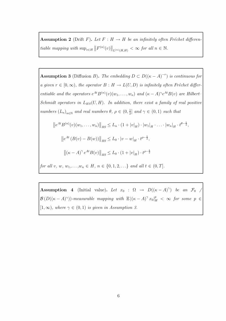
Assumption 2 (Drift F ). Let F : H → H be an infinitely often Frechet differen-
tiable mapping with supv∈H
∥
∥F (n)(v)∥
∥
L(n)(H,H)< ∞ for all n ∈ N.
Assumption 3 (Diffusion B). The embedding D ⊂ D((κ− A)−r
) is continuous for
a given r ∈ [0,∞), the operator B : H → L(U,D) is infinitely often Frechet differ-
entiable and the operators eAtB(n)(v)(w1, . . . , wn) and (κ−A)γeAtB(v) are Hilbert–
Schmidt operators in LHS(U,H). In addition, there exist a family of real positive
numbers (Ln)n∈Nand real numbers θ, ρ ∈ (0, 1
2] and γ ∈ (0, 1) such that
∥
∥eAtB(n)(v)(w1, . . . , wn)∥
∥
HS≤ Ln · (1 + |v|H) · |w1|H · . . . · |wn|H · tθ−
1
2 ,
∥
∥eAt (B(v) − B(w))∥
∥
HS≤ L0 · |v − w|H · tρ−
1
2 ,
∥
∥(κ− A)γeAtB(v)
∥
∥
HS≤ L0 · (1 + |v|H) · tρ−
1
2
for all v, w, w1,. . . ,wn ∈ H, n ∈ 0, 1, 2, . . . and all t ∈ (0, T ].
Assumption 4 (Initial value). Let x0 : Ω → D((κ−A)γ) be an F0 /
B (D((κ− A)γ))-measurable mapping with E |(κ− A)γx0|
p
H < ∞ for some p ∈
[1,∞), where γ ∈ (0, 1) is given in Assumption 3.
6

Consider the SPDE
dXt =
[
AXt + F (Xt)
]
dt+B(Xt) dWt, X0 = x0 (6)
for t ∈ [0, T ].
Under Assumptions 1–4 the SPDE (6) has a unique mild solution.
Proposition 1. Let Assumptions 1–4 be satisfied and let γ ∈ (0, 1) be given by
Assumption 3. Then there is an up to modifications unique predictable stochastic
process X : [0, T ]×Ω → D((κ−A)γ) with sup0≤t≤T E |(κ− A)γXt|
p
H < ∞ such that
P
[
Xt = eAtx0 +
∫ t
0
eA(t−s)F (Xs) ds+
∫ t
0
eA(t−s)B(Xs) dWs
]
= 1 (7)
for all t ∈ [0, T ].
Moreover, X is the unique mild solution of the SPDE (6) in the sense of equation
(7).
Reference
A. Jentzen, Taylor expansions of solutions of stochastic partial differential equa-
tions, Discrete & Cont. Dyn. Systems Series B 14 (2010), 515–557.
7
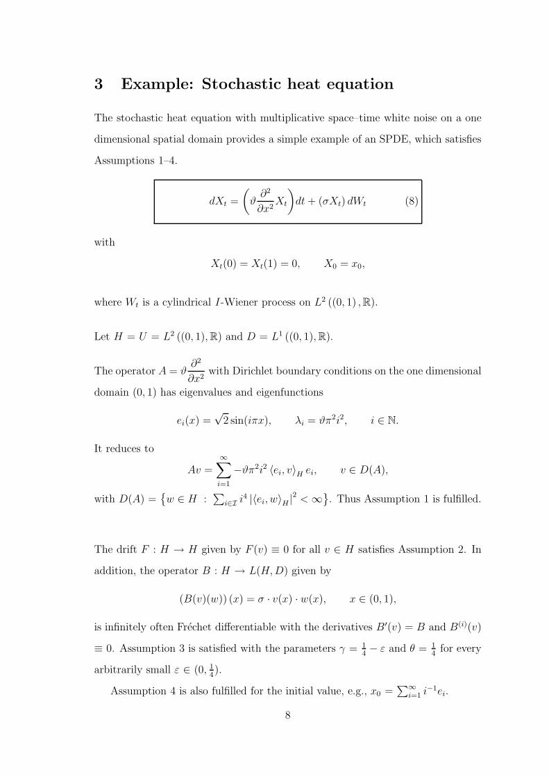
3 Example: Stochastic heat equation
The stochastic heat equation with multiplicative space–time white noise on a one
dimensional spatial domain provides a simple example of an SPDE, which satisfies
Assumptions 1–4.
dXt =
(
ϑ∂2
∂x2Xt
)
dt+ (σXt) dWt (8)
with
Xt(0) = Xt(1) = 0, X0 = x0,
where Wt is a cylindrical I-Wiener process on L2 ((0, 1) ,R).
Let H = U = L2 ((0, 1),R) and D = L1 ((0, 1),R).
The operator A = ϑ∂2
∂x2with Dirichlet boundary conditions on the one dimensional
domain (0, 1) has eigenvalues and eigenfunctions
ei(x) =√
2 sin(iπx), λi = ϑπ2i2, i ∈ N.
It reduces to
Av =
∞∑
i=1
−ϑπ2i2 〈ei, v〉H ei, v ∈ D(A),
with D(A) =
w ∈ H :∑
i∈I i4 |〈ei, w〉H |
2<∞
. Thus Assumption 1 is fulfilled.
The drift F : H → H given by F (v) ≡ 0 for all v ∈ H satisfies Assumption 2. In
addition, the operator B : H → L(H,D) given by
(B(v)(w)) (x) = σ · v(x) · w(x), x ∈ (0, 1),
is infinitely often Frechet differentiable with the derivatives B′(v) = B and B(i)(v)
≡ 0. Assumption 3 is satisfied with the parameters γ = 14− ε and θ = 1
4for every
arbitrarily small ε ∈ (0, 14).
Assumption 4 is also fulfilled for the initial value, e.g., x0 =∑∞
i=1 i−1ei.
8
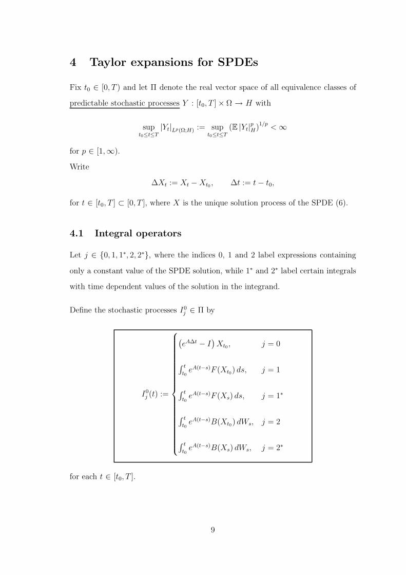
4 Taylor expansions for SPDEs
Fix t0 ∈ [0, T ) and let Π denote the real vector space of all equivalence classes of
predictable stochastic processes Y : [t0, T ] × Ω → H with
supt0≤t≤T
|Yt|Lp(Ω;H) := supt0≤t≤T
(E |Yt|p
H)1/p
<∞
for p ∈ [1,∞).
Write
∆Xt := Xt −Xt0 , ∆t := t− t0,
for t ∈ [t0, T ] ⊂ [0, T ], where X is the unique solution process of the SPDE (6).
4.1 Integral operators
Let j ∈ 0, 1, 1∗, 2, 2∗, where the indices 0, 1 and 2 label expressions containing
only a constant value of the SPDE solution, while 1∗ and 2∗ label certain integrals
with time dependent values of the solution in the integrand.
Define the stochastic processes I0j ∈ Π by
I0j (t) :=
(
eA∆t − I)
Xt0 , j = 0
∫ t
t0eA(t−s)F (Xt0) ds, j = 1
∫ t
t0eA(t−s)F (Xs) ds, j = 1∗
∫ t
t0eA(t−s)B(Xt0) dWs, j = 2
∫ t
t0eA(t−s)B(Xs) dWs, j = 2∗
for each t ∈ [t0, T ].
9
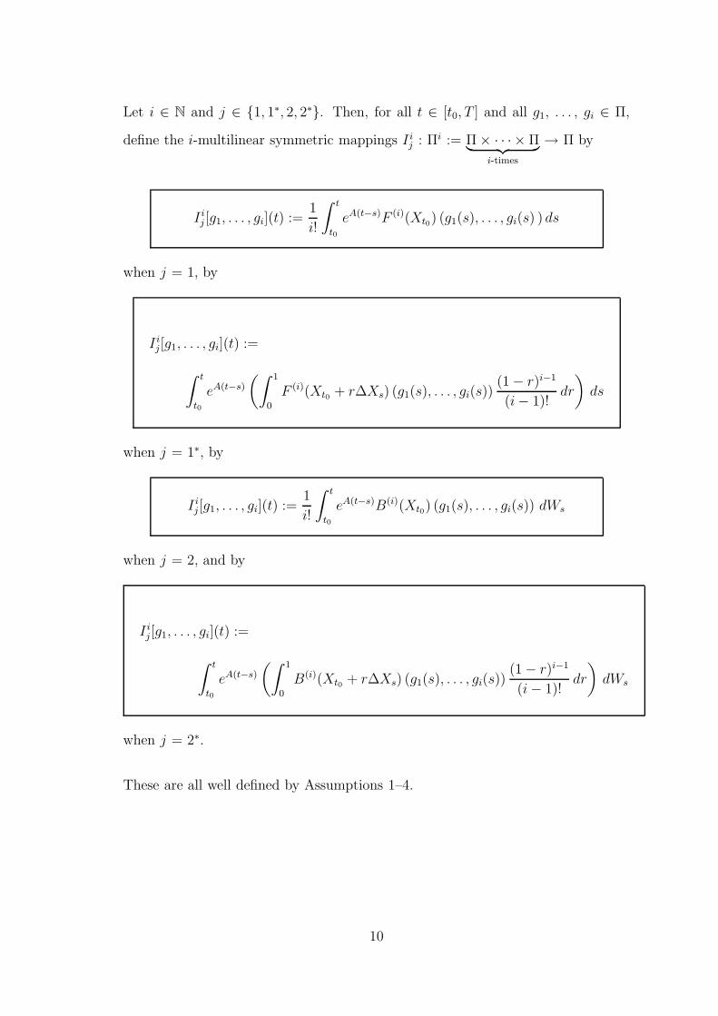
Let i ∈ N and j ∈ 1, 1∗, 2, 2∗. Then, for all t ∈ [t0, T ] and all g1, . . . , gi ∈ Π,
define the i-multilinear symmetric mappings I ij : Πi := Π × · · · × Π
︸ ︷︷ ︸
i-times
→ Π by
I ij [g1, . . . , gi](t) :=
1
i!
∫ t
t0
eA(t−s)F (i)(Xt0) (g1(s), . . . , gi(s) ) ds
when j = 1, by
I ij[g1, . . . , gi](t) :=
∫ t
t0
eA(t−s)
(∫ 1
0
F (i)(Xt0 + r∆Xs) (g1(s), . . . , gi(s))(1 − r)i−1
(i− 1)!dr
)
ds
when j = 1∗, by
I ij[g1, . . . , gi](t) :=
1
i!
∫ t
t0
eA(t−s)B(i)(Xt0) (g1(s), . . . , gi(s)) dWs
when j = 2, and by
I ij[g1, . . . , gi](t) :=
∫ t
t0
eA(t−s)
(∫ 1
0
B(i)(Xt0 + r∆Xs) (g1(s), . . . , gi(s))(1 − r)i−1
(i− 1)!dr
)
dWs
when j = 2∗.
These are all well defined by Assumptions 1–4.
10
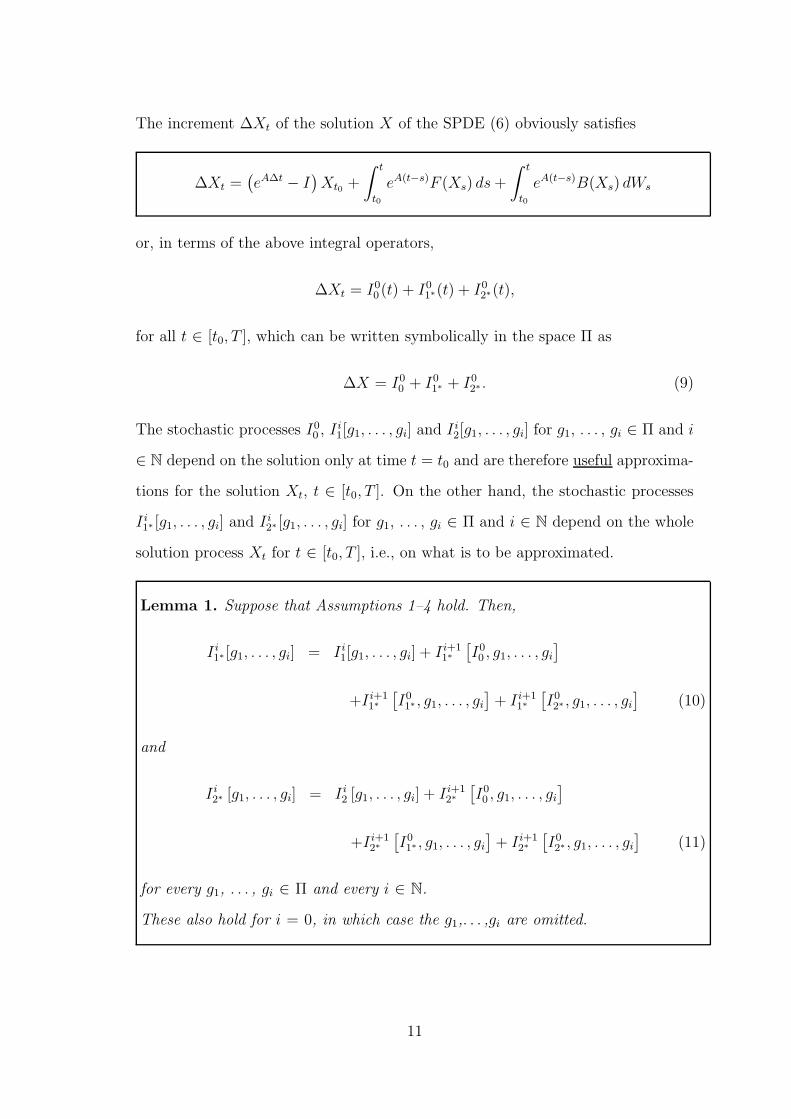
The increment ∆Xt of the solution X of the SPDE (6) obviously satisfies
∆Xt =(
eA∆t − I)
Xt0 +
∫ t
t0
eA(t−s)F (Xs) ds+
∫ t
t0
eA(t−s)B(Xs) dWs
or, in terms of the above integral operators,
∆Xt = I00 (t) + I0
1∗(t) + I02∗(t),
for all t ∈ [t0, T ], which can be written symbolically in the space Π as
∆X = I00 + I0
1∗ + I02∗ . (9)
The stochastic processes I00 , I i
1[g1, . . . , gi] and I i2[g1, . . . , gi] for g1, . . . , gi ∈ Π and i
∈ N depend on the solution only at time t = t0 and are therefore useful approxima-
tions for the solution Xt, t ∈ [t0, T ]. On the other hand, the stochastic processes
I i1∗ [g1, . . . , gi] and I i
2∗ [g1, . . . , gi] for g1, . . . , gi ∈ Π and i ∈ N depend on the whole
solution process Xt for t ∈ [t0, T ], i.e., on what is to be approximated.
Lemma 1. Suppose that Assumptions 1–4 hold. Then,
I i1∗ [g1, . . . , gi] = I i
1[g1, . . . , gi] + I i+11∗
[
I00 , g1, . . . , gi
]
+I i+11∗
[
I01∗ , g1, . . . , gi
]
+ I i+11∗
[
I02∗ , g1, . . . , gi
]
(10)
and
I i2∗ [g1, . . . , gi] = I i
2 [g1, . . . , gi] + I i+12∗
[
I00 , g1, . . . , gi
]
+I i+12∗
[
I01∗ , g1, . . . , gi
]
+ I i+12∗
[
I02∗ , g1, . . . , gi
]
(11)
for every g1, . . . , gi ∈ Π and every i ∈ N.
These also hold for i = 0, in which case the g1,. . . ,gi are omitted.
11
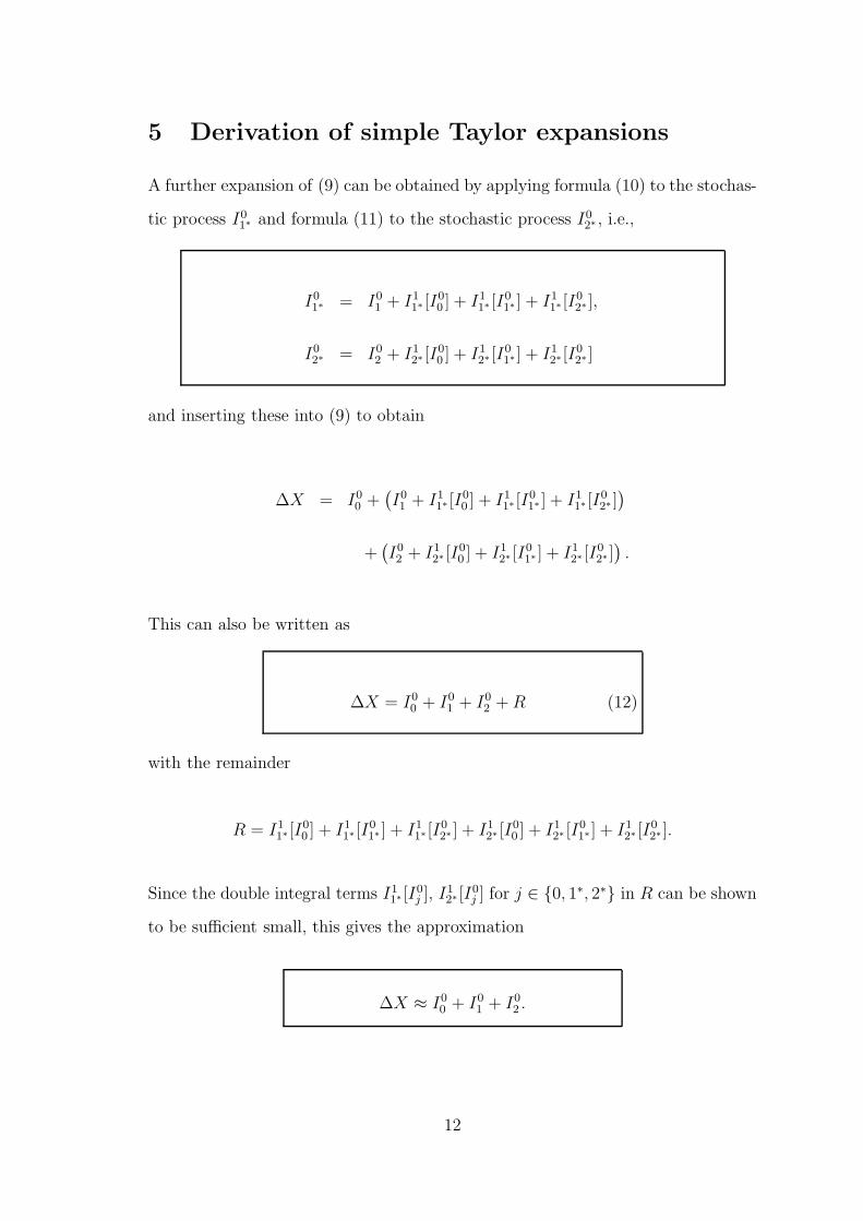
5 Derivation of simple Taylor expansions
A further expansion of (9) can be obtained by applying formula (10) to the stochas-
tic process I01∗ and formula (11) to the stochastic process I0
2∗ , i.e.,
I01∗ = I0
1 + I11∗ [I
00 ] + I1
1∗ [I01∗ ] + I1
1∗ [I02∗ ],
I02∗ = I0
2 + I12∗ [I
00 ] + I1
2∗ [I01∗ ] + I1
2∗ [I02∗ ]
and inserting these into (9) to obtain
∆X = I00 +
(
I01 + I1
1∗ [I00 ] + I1
1∗ [I01∗ ] + I1
1∗ [I02∗ ])
+(
I02 + I1
2∗ [I00 ] + I1
2∗ [I01∗ ] + I1
2∗ [I02∗ ])
.
This can also be written as
∆X = I00 + I0
1 + I02 +R (12)
with the remainder
R = I11∗ [I
00 ] + I1
1∗ [I01∗ ] + I1
1∗ [I02∗ ] + I1
2∗ [I00 ] + I1
2∗ [I01∗ ] + I1
2∗ [I02∗ ].
Since the double integral terms I11∗ [I
0j ], I1
2∗ [I0j ] for j ∈ 0, 1∗, 2∗ in R can be shown
to be sufficient small, this gives the approximation
∆X ≈ I00 + I0
1 + I02 .
12
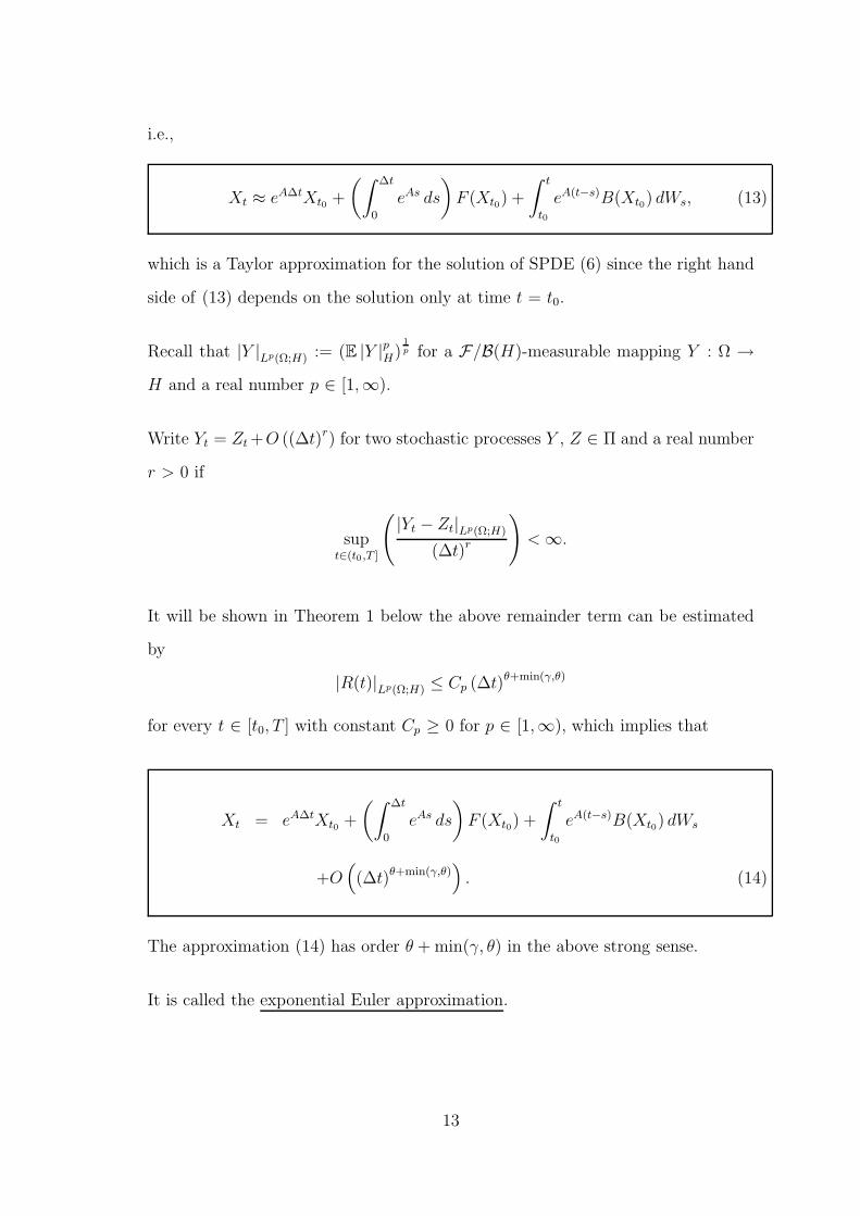
i.e.,
Xt ≈ eA∆tXt0 +
(∫ ∆t
0
eAs ds
)
F (Xt0) +
∫ t
t0
eA(t−s)B(Xt0) dWs, (13)
which is a Taylor approximation for the solution of SPDE (6) since the right hand
side of (13) depends on the solution only at time t = t0.
Recall that |Y |Lp(Ω;H) := (E |Y |pH)1
p for a F/B(H)-measurable mapping Y : Ω →
H and a real number p ∈ [1,∞).
Write Yt = Zt +O ((∆t)r) for two stochastic processes Y , Z ∈ Π and a real number
r > 0 if
supt∈(t0,T ]
(
|Yt − Zt|Lp(Ω;H)
(∆t)r
)
<∞.
It will be shown in Theorem 1 below the above remainder term can be estimated
by
|R(t)|Lp(Ω;H) ≤ Cp (∆t)θ+min(γ,θ)
for every t ∈ [t0, T ] with constant Cp ≥ 0 for p ∈ [1,∞), which implies that
Xt = eA∆tXt0 +
(∫ ∆t
0
eAs ds
)
F (Xt0) +
∫ t
t0
eA(t−s)B(Xt0) dWs
+O(
(∆t)θ+min(γ,θ)
)
. (14)
The approximation (14) has order θ + min(γ, θ) in the above strong sense.
It is called the exponential Euler approximation.
13
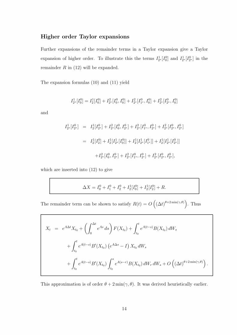
Higher order Taylor expansions
Further expansions of the remainder terms in a Taylor expansion give a Taylor
expansion of higher order. To illustrate this the terms I12∗ [I
00 ] and I1
2∗ [I02∗ ] in the
remainder R in (12) will be expanded.
The expansion formulas (10) and (11) yield
I12∗ [I
00 ] = I1
2 [I00 ] + I2
2∗ [I00 , I
00 ] + I2
2∗ [I01∗ , I
00 ] + I2
2∗ [I02∗ , I
00 ]
and
I12∗ [I
02∗ ] = I1
2 [I02∗ ] + I2
2∗ [I00 , I
02∗ ] + I2
2∗ [I01∗ , I
02∗ ] + I2
2∗ [I02∗ , I
02∗ ]
= I12 [I0
2 ] + I12 [I1
2∗ [I00 ]] + I1
2 [I12∗ [I
01∗ ]] + I1
2 [I12∗ [I
02∗ ]]
+I22∗ [I
00 , I
02∗ ] + I2
2∗ [I01∗ , I
02∗ ] + I2
2∗ [I02∗ , I
02∗ ],
which are inserted into (12) to give
∆X = I00 + I0
1 + I02 + I1
2 [I00 ] + I1
2 [I02 ] +R.
The remainder term can be shown to satisfy R(t) = O(
(∆t)θ+2min(γ,θ)
)
. Thus
Xt = eA∆tXt0 +
(∫ ∆t
0
eAs ds
)
F (Xt0) +
∫ t
t0
eA(t−s)B(Xt0) dWs
+
∫ t
t0
eA(t−s)B′(Xt0)(
eA∆s − I)
Xt0 dWs
+
∫ t
t0
eA(t−s)B′(Xt0)
∫ s
t0
eA(s−r)B(Xt0) dWr dWs +O(
(∆t)θ+2min(γ,θ)
)
.
This approximation is of order θ + 2 min(γ, θ). It was derived heuristically earlier.
14
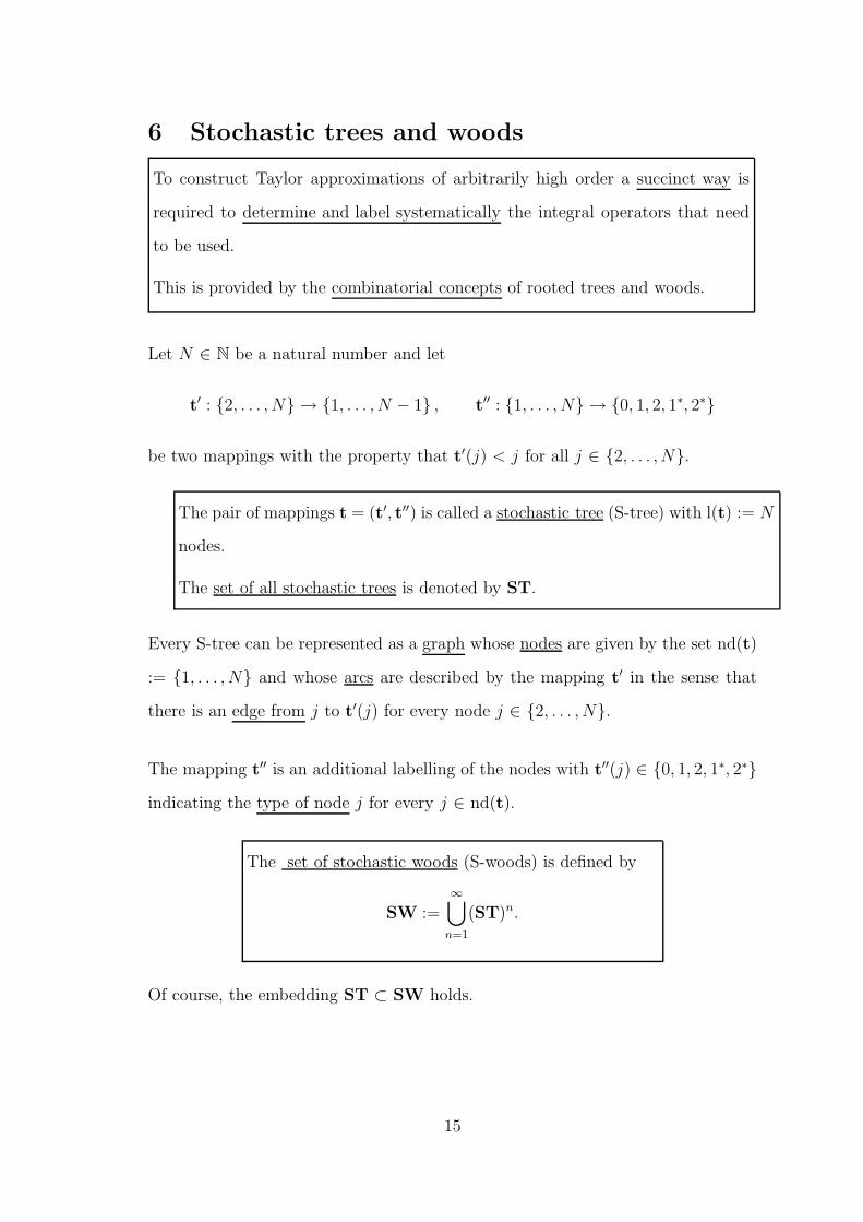
6 Stochastic trees and woods
To construct Taylor approximations of arbitrarily high order a succinct way is
required to determine and label systematically the integral operators that need
to be used.
This is provided by the combinatorial concepts of rooted trees and woods.
Let N ∈ N be a natural number and let
t′ : 2, . . . , N → 1, . . . , N − 1 , t′′ : 1, . . . , N → 0, 1, 2, 1∗, 2∗
be two mappings with the property that t′(j) < j for all j ∈ 2, . . . , N.
The pair of mappings t = (t′, t′′) is called a stochastic tree (S-tree) with l(t) := N
nodes.
The set of all stochastic trees is denoted by ST.
Every S-tree can be represented as a graph whose nodes are given by the set nd(t)
:= 1, . . . , N and whose arcs are described by the mapping t′ in the sense that
there is an edge from j to t′(j) for every node j ∈ 2, . . . , N.
The mapping t′′ is an additional labelling of the nodes with t′′(j) ∈ 0, 1, 2, 1∗, 2∗
indicating the type of node j for every j ∈ nd(t).
The set of stochastic woods (S-woods) is defined by
SW :=
∞⋃
n=1
(ST)n.
Of course, the embedding ST ⊂ SW holds.
15
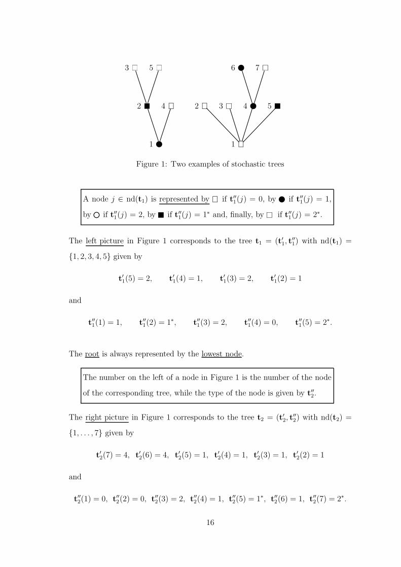
1 b
2 r
3 rs 5 rs
4 ⊗
1 ⊗
2 ⊗ 3 rs 4 b
6 b 7 rs
5 r
Figure 1: Two examples of stochastic trees
A node j ∈ nd(t1) is represented by ⊗ if t′′1(j) = 0, by b if t′′1(j) = 1,
by bCif t′′1(j) = 2, by r if t′′1(j) = 1∗ and, finally, by rs if t′′1(j) = 2∗.
The left picture in Figure 1 corresponds to the tree t1 = (t′1, t′′1) with nd(t1) =
1, 2, 3, 4, 5 given by
t′1(5) = 2, t′1(4) = 1, t′1(3) = 2, t′1(2) = 1
and
t′′1(1) = 1, t′′1(2) = 1∗, t′′1(3) = 2, t′′1(4) = 0, t′′1(5) = 2∗.
The root is always represented by the lowest node.
The number on the left of a node in Figure 1 is the number of the node
of the corresponding tree, while the type of the node is given by t′′2.
The right picture in Figure 1 corresponds to the tree t2 = (t′2, t′′2) with nd(t2) =
1, . . . , 7 given by
t′2(7) = 4, t′2(6) = 4, t′2(5) = 1, t′2(4) = 1, t′2(3) = 1, t′2(2) = 1
and
t′′2(1) = 0, t′′2(2) = 0, t′′2(3) = 2, t′′2(4) = 1, t′′2(5) = 1∗, t′′2(6) = 1, t′′2(7) = 2∗.
16
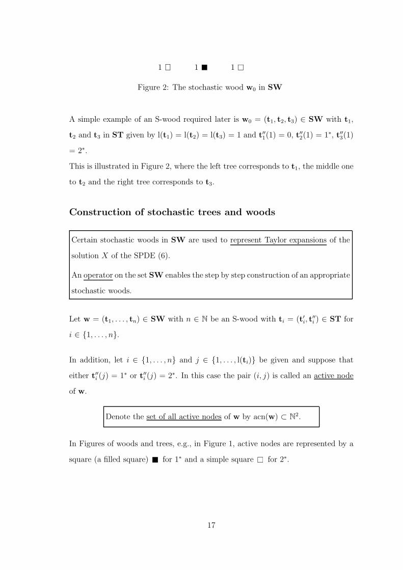
1 ⊗ 1 r 1 rs
Figure 2: The stochastic wood w0 in SW
A simple example of an S-wood required later is w0 = (t1, t2, t3) ∈ SW with t1,
t2 and t3 in ST given by l(t1) = l(t2) = l(t3) = 1 and t′′1(1) = 0, t′′2(1) = 1∗, t′′3(1)
= 2∗.
This is illustrated in Figure 2, where the left tree corresponds to t1, the middle one
to t2 and the right tree corresponds to t3.
Construction of stochastic trees and woods
Certain stochastic woods in SW are used to represent Taylor expansions of the
solution X of the SPDE (6).
An operator on the set SW enables the step by step construction of an appropriate
stochastic woods.
Let w = (t1, . . . , tn) ∈ SW with n ∈ N be an S-wood with ti = (t′i, t′′i ) ∈ ST for
i ∈ 1, . . . , n.
In addition, let i ∈ 1, . . . , n and j ∈ 1, . . . , l(ti) be given and suppose that
either t′′i (j) = 1∗ or t′′i (j) = 2∗. In this case the pair (i, j) is called an active node
of w.
Denote the set of all active nodes of w by acn(w) ⊂ N2.
In Figures of woods and trees, e.g., in Figure 1, active nodes are represented by a
square (a filled square) r for 1∗ and a simple square rs for 2∗.
17
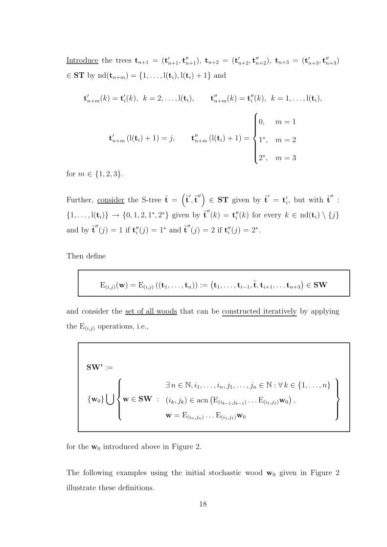
Introduce the trees tn+1 = (t′n+1, t′′n+1), tn+2 = (t′n+2, t
′′n+2), tn+3 = (t′n+3, t
′′n+3)
∈ ST by nd(tn+m) = 1, . . . , l(ti), l(ti) + 1 and
t′n+m(k) = t′i(k), k = 2, . . . , l(ti), t′′n+m(k) = t′′i (k), k = 1, . . . , l(ti),
t′n+m (l(ti) + 1) = j, t′′n+m (l(ti) + 1) =
0, m = 1
1∗, m = 2
2∗, m = 3
for m ∈ 1, 2, 3.
Further, consider the S-tree t =(
t′, t
′′)
∈ ST given by t′
= t′i, but with t′′
:
1, . . . , l(ti) → 0, 1, 2, 1∗, 2∗ given by t′′(k) = t′′i (k) for every k ∈ nd(ti) \ j
and by t′′(j) = 1 if t′′i (j) = 1∗ and t
′′(j) = 2 if t′′i (j) = 2∗.
Then define
E(i,j)(w) = E(i,j) ((t1, . . . , tn)) :=(
t1, . . . , ti−1, t, ti+1, . . . tn+3
)
∈ SW
and consider the set of all woods that can be constructed iteratively by applying
the E(i,j) operations, i.e.,
SW’ :=
w0⋃
w ∈ SW :
∃n ∈ N, i1, . . . , in, j1, . . . , jn ∈ N : ∀ k ∈ 1, . . . , n
(ik, jk) ∈ acn(
E(ik−1,jk−1) . . .E(i1,j1)w0
)
,
w = E(in,jn) . . .E(i1,j1)w0
for the w0 introduced above in Figure 2.
The following examples using the initial stochastic wood w0 given in Figure 2
illustrate these definitions.
18
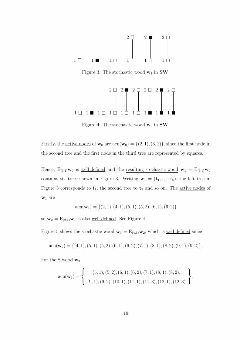
1 ⊗ 1 r 1 rs 1 rs
2 ⊗
1 rs
2 r
1 rs
2 rs
Figure 3: The stochastic wood w1 in SW
1 ⊗ 1 r 1 rs 1 rs
2 ⊗
1 rs
2 r
1 rs
2 rs
1 r
2 ⊗
1 r
2 r
1 r
2 rs
Figure 4: The stochastic wood w2 in SW
Firstly, the active nodes of w0 are acn(w0) = (2, 1), (3, 1), since the first node in
the second tree and the first node in the third tree are represented by squares.
Hence, E(3,1)w0 is well defined and the resulting stochastic wood w1 = E(3,1)w0
contains six trees shown in Figure 3. Writing w1 = (t1, . . . , t6), the left tree in
Figure 3 corresponds to t1, the second tree to t2 and so on. The active nodes of
w1 are
acn(w1) = (2, 1), (4, 1), (5, 1), (5, 2), (6, 1), (6, 2)
so w2 = E(2,1)w1 is also well defined. See Figure 4.
Figure 5 shows the stochastic wood w3 = E(4,1)w2, which is well defined since
acn(w2) = (4, 1), (5, 1), (5, 2), (6, 1), (6, 2), (7, 1), (8, 1), (8, 2), (9, 1), (9, 2) .
For the S-wood w3
acn(w3) =
(5, 1), (5, 2), (6, 1), (6, 2), (7, 1), (8, 1), (8, 2),
(9, 1), (9, 2), (10, 1), (11, 1), (11, 3), (12, 1), (12, 3)
.
19
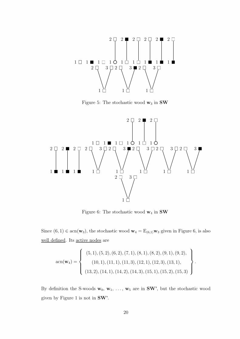
1 ⊗ 1 r 1 rs 1 bC
2 ⊗
1 rs
2 r
1 rs
2 rs
1 r
2 ⊗
1 r
2 r
1 r
2 rs
1 rs
2 ⊗ 3 ⊗
1 rs
2 ⊗ 3 r
1 rs
2 ⊗ 3 rs
Figure 5: The stochastic wood w3 in SW
1 ⊗ 1 r 1 rs 1 bC
2 ⊗
1 rs
2 r
1 bC
2 rs
1 r
2 ⊗
1 r
2 r
1 r
2 rs
1 rs
2 ⊗ 3 ⊗
1 rs
2 ⊗ 3 r
1 rs
2 ⊗ 3 rs
1 rs
2 rs 3 ⊗
1 rs
2 rs 3 r
1 rs
2 rs 3 rs
Figure 6: The stochastic wood w4 in SW
Since (6, 1) ∈ acn(w3), the stochastic wood w4 = E(6,1)w3 given in Figure 6, is also
well defined. Its active nodes are
acn(w4) =
(5, 1), (5, 2), (6, 2), (7, 1), (8, 1), (8, 2), (9, 1), (9, 2),
(10, 1), (11, 1), (11, 3), (12, 1), (12, 3), (13, 1),
(13, 2), (14, 1), (14, 2), (14, 3), (15, 1), (15, 2), (15, 3)
.
By definition the S-woods w0, w1, . . . , w5 are in SW’, but the stochastic wood
given by Figure 1 is not in SW’.
20
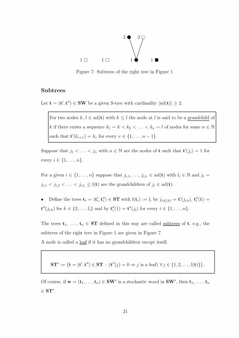
1 ⊗ 1 rs 1 b
2 b 3 rs
1 r
Figure 7: Subtrees of the right tree in Figure 1
Subtrees
Let t = (t′, t′′) ∈ SW be a given S-tree with cardinality |nd(t)| ≥ 2.
For two nodes k, l ∈ nd(t) with k ≤ l the node at l is said to be a grandchild of
k if there exists a sequence k1 = k < k2 < . . . < kn = l of nodes for some n ∈ N
such that t′(kv+1) = kv for every v ∈ 1, . . . , n− 1.
Suppose that j1 < . . . < jn with n ∈ N are the nodes of t such that t′(ji) = 1 for
every i ∈ 1, . . . , n.
For a given i ∈ 1, . . . , n suppose that ji,1, . . ., ji,li ∈ nd(t) with li ∈ N and ji =
ji,1 < ji,2 < . . . < ji,li ≤ l(t) are the grandchildren of ji ∈ nd(t).
• Define the trees ti = (t′i, t′′i ) ∈ ST with l(ti) := li by ji,t′i(k) = t′(ji,k), t′′i (k) =
t′′(ji,k) for k ∈ 2, . . . , li and by t′′i (1) = t′′(ji) for every i ∈ 1, . . . , n.
The trees t1, . . . , tn ∈ ST defined in this way are called subtrees of t, e.g., the
subtrees of the right tree in Figure 1 are given in Figure 7.
A node is called a leaf if it has no grandchildren except itself.
ST’ := t = (t′, t′′) ∈ ST : (t′′(j) = 0 ⇒ j is a leaf) ∀ j ∈ 1, 2, . . . , l(t) .
Of course, if w = (t1, . . . , tn) ∈ SW’ is a stochastic wood in SW’, then t1, . . . , tn
∈ ST’.
21

Order of stochastic trees and woods
The order of an S-tree t ∈ ST’ is given by the function ordt : ST’ → [0,∞)
ordt(t) := |j ∈ nd(t) : t′′(j) = 1 or t′′(j) = 1∗|
+γ |j ∈ nd(t) : t′′(j) = 0| + θ |j ∈ nd(t) : t′′(j) = 2 or t′′(j) = 2∗|
for every S-tree t = (t′, t′′) ∈ ST’.
Example The order of the left tree in Figure 1 is 2+γ+2θ since the left tree has
one node of type 0, two nodes of type 1 and type 1∗, and also two nodes of type 2
and type 2∗.
A tree t = (t′, t′′) ∈ ST’ is said to be active if there is a j ∈ nd(t) such that t′′(j)
= 1∗ or t′′(j) = 2∗, i.e., an S-tree is active if it has an active node.
The order of an S-wood w ∈ SW’ is given by the function ord : SW’ → [0,∞)
ord(w) := min ordt(ti) ∈ [0,∞) : i ∈ 1, . . . , n such that ti is active
for every S-wood w = (t1, . . . , tn) ∈ SW’ with n ∈ N.
ord(w0) = min1, θ = θ
ord(w1) = min1, θ + γ, θ + 1, = θ + min(γ, θ)
ord(w2) = minθ + γ, θ + 1, 2θ, 1 + γ, 2, 1 + θ = θ + min(θ, γ)
ord(w3) = θ + min(θ, 2γ) = ord(w4)
ord(w5) = w5θ + 2 min(θ, γ)
22
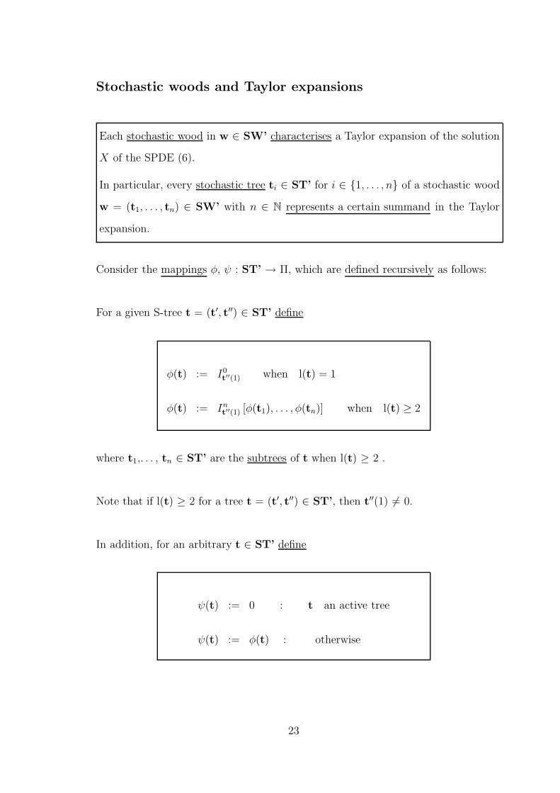
Stochastic woods and Taylor expansions
Each stochastic wood in w ∈ SW’ characterises a Taylor expansion of the solution
X of the SPDE (6).
In particular, every stochastic tree ti ∈ ST’ for i ∈ 1, . . . , n of a stochastic wood
w = (t1, . . . , tn) ∈ SW’ with n ∈ N represents a certain summand in the Taylor
expansion.
Consider the mappings φ, ψ : ST’ → Π, which are defined recursively as follows:
For a given S-tree t = (t′, t′′) ∈ ST’ define
φ(t) := I0t′′(1) when l(t) = 1
φ(t) := Int′′(1) [φ(t1), . . . , φ(tn)] when l(t) ≥ 2
where t1,. . . , tn ∈ ST’ are the subtrees of t when l(t) ≥ 2 .
Note that if l(t) ≥ 2 for a tree t = (t′, t′′) ∈ ST’, then t′′(1) 6= 0.
In addition, for an arbitrary t ∈ ST’ define
ψ(t) := 0 : t an active tree
ψ(t) := φ(t) : otherwise
23

Finally, define mappings Φ, Ψ : SW’ → Π by
Φ(w) = φ(t1) + . . .+ φ(tn), Ψ(w) = ψ(t1) + . . .+ ψ(tn)
for every S-wood w = (t1, . . . , tn) ∈ SW’ with n ∈ N.
For example, for the initial stochastic wood w0 (see Figure 2)
Φ(w0) = I00 + I0
1∗ + I02∗ , Ψ(w0) = I0
0 . (15)
Hence, Φ(w0) = ∆X from (15) and (9).
Furthermore,
Φ(w1) = I00 + I0
1∗ + I02 + I1
2∗ [I00 ] + I1
2∗ [I01∗ ] + I1
2∗ [I02∗ ] (16)
and
Ψ(w1) = I00 + I0
2 (17)
Each stochastic wood w ∈ SW’ thus represents a Taylor expansion
Xt0 + Φ(w)(t)
and the corresponding Taylor approximation
Xt0 + Ψ(w)(t)
for t ∈ [t0, T ] of the solution process X of the SPDE (6).
24

Theorem 1. Let Assumptions 1–4 be fulfilled, let w ∈ SW’. Then there exists a
constant Cp > 0 such that
P
[
Xt = Xt0 + Φ(w) (t)
]
= 1,
and(
E
[
∣
∣Xt −Xt0 − Ψ(w)(t)∣
∣
p
H
])1
p
≤ Cp (t− t0)ord(w)
holds for every t ∈ [t0, T ], where X is the up to modifications unique solution of the
SPDE (6).
The constant Cp here only depends on the S-wood w, p and the coefficients of the
SPDE.
The Taylor approximation in Theorem 1 can also be written as
Xt = Xt0 + Ψ(w) +O(
(∆t)ord(w)
)
(18)
for every stochastic wood w ∈ SW’.
The following lemma shows that there are woods in SW’ with arbitrarily high
orders.
Lemma 2. Let Assumptions 1–4 be fulfilled. Then
supw∈SW’
ord (w) = ∞.
Thus Taylor approximations of arbitrarily high orders can be constructed by suc-
cessively applying the E(i,j) operator.
25
7 Examples of Taylor approximations
Taylor approximationsXt0+Ψ(w)(t) in Theorem 1 and (18) based on the stochastic
woods w ∈ w0,w1, . . . ,w5 are presented here. Theorem 1 gives
(
E
[
∣
∣Xt −Xt0 − Ψ(w)(t)∣
∣
p
H
])1
p
≤ Cp (∆t)ord(w)
for every t ∈ [t0, T ] and appropriate constant Cp > 0, where p ∈ [1,∞).
The orders of the Taylor approximations here depend on the two parameters θ ∈
(0, 12] and γ ∈ (0, 1) in Assumption 3.
Taylor approximation of order θ
The first Taylor expansion of the solution is given by the initial stochastic wood w0
(see Figure 2), i.e., Φ(w0) = ∆X is approximated by Ψ(w0) with order ord(w0).
Specifically, by (15),
Ψ(w0)(t) = (eA∆t − I)Xt0 ,
and
Φ(w0)(t) = (eA∆t − I)Xt0 +
∫ t
t0
eA(t−s)F (Xs) ds+
∫ t
t0
eA(t−s)B(Xs) dWs
for every t ∈ [t0, T ].
Since ord(w0) = θ, the corresponding Taylor approximation
Xt = eA∆tXt0 +O(
(∆t)θ)
(19)
has order θ.
26
Two Taylor approximations of order θ + min(γ, θ)
Consider the Taylor approximation given by the S-wood w1 (see Figure 3) is based
on Φ(w1) and Ψ(w1), which were given in (16) and (17).
Since ord(w1) = θ + min(γ, θ), the Taylor approximation
Xt = eA∆tXt0 +
∫ t
t0
eA(t−s)B(Xt0) dWs +O(
(∆t)θ+min(γ,θ)
)
(20)
has order θ + min(γ, θ).
The stochastic wood w2 (see Figure 4) has order θ + min(γ, θ) and the Taylor
approximation Ψ(w2) of Φ(w2) = ∆X is given by Ψ(w2) = I00 + I0
1 + I02 , i.e.,
Xt = eA∆tXt0 +
(∫ ∆t
0
eAs ds
)
F (Xt0) +
∫ t
t0
eA(t−s)B(Xt0) dWs (21)
+O(
(∆t)θ+min(γ,θ)
)
.
This approximation of order θ+ min(γ, θ) is the exponential Euler approximation.
It is natural to ask is why one should use the Taylor approximation (21) if it is of
the same order as the Taylor approximation (20).
Although both of these Taylor approximations have the same local approximation
order, for numerical schemes it is the global approximation order and behaviour
that are of primary importance, as will be discussed in subsection 9.
It turns out that the exponential Euler scheme based on the Taylor approximation
(21) has very good global approximation properties.
27
Taylor approximation of order θ + min(2γ, θ)
The stochastic wood w3 (see Figure 5) has order θ + min(2γ, θ) and
Ψ(w3) = I00 + I0
1 + I02 + I1
2 [I00 ].
The corresponding Taylor approximation
Xt = eA∆tXt0 +
(∫ ∆t
0
eAs ds
)
F (Xt0) +
∫ t
t0
eA(t−s)B(Xt0) dWs (22)
+
∫ t
t0
eA(t−s)B′(Xt0)((
eA∆s − I)
Xt0
)
dWs +O(
(∆t)θ+min(2γ,θ)
)
thus has order θ + min(2γ, θ).
Note that the stochastic woods w3 and w4 give the same Taylor approximation,
i.e., Ψ(w4) = Ψ(w3).
Taylor approximation of order θ + 2 min(γ, θ)
The Taylor approximation corresponding to the S-wood w5 is
Xt = eA∆tXt0 +
(∫ ∆t
0
eAs ds
)
F (Xt0) +
∫ t
t0
eA(t−s)B(Xt0) dWs
+
∫ t
t0
eA(t−s)B′(Xt0)
∫ s
t0
eA(s−r)B(Xt0) dWr dWs (23)
+
∫ t
t0
eA(t−s)B′(Xt0)((
eA∆s − I)
Xt0
)
dWs +O(
(∆t)θ+2min(γ,θ)
)
and thus has order θ + 2 min(γ, θ).
28
7.1 Application to the stochastic heat equation
The stochastic heat equation (8) satisfies the Assumptions 1–4 with the parameters
θ = 14
and γ = 14− ε for arbitrarily small ε ∈ (0, 1
4).
The Taylor approximations below exploit the special structure of the stochastic
heat equation, i.e., its drift term vanishes and its diffusion term is linear.
The Taylor approximations (20), (22) and (23) reduce to
Xt = eA∆tXt0 +
∫ t
t0
eA(t−s)B(Xt0) dWs +O(
(∆t)1
2−ε)
.
Xt = eA∆tXt0 +
∫ t
t0
eA(t−s)B(Xt0) dWs
+
∫ t
t0
eA(t−s)B((eA∆s − I)Xt0) dWs +O(
(∆t)1
2
)
= eA∆tXt0 +
∫ t
t0
eA(t−s)B(eA∆sXt0) dWs +O(
(∆t)1
2
)
.
Xt = eA∆tXt0 +
∫ t
t0
eA(t−s)B(eA∆sXt0) dWs
+
∫ t
t0
eA(t−s)B
(∫ s
t0
eA(s−r)B(Xt0) dWr
)
dWs + O(
(∆t)3
4−ε)
= eA∆tXt0 +
∫ t
t0
eA(t−s)B
(
eA∆sXt0 +
∫ s
t0
eA(s−r)B(Xt0) dWr
)
dWs
+ O(
(∆t)3
4−ε)
.
29
7.2 Finite dimensional SODEs
The abstract setting for SPDE here includes finite dimensional SODEs.
Let U = H = R and let Wt be a standard scalar Wiener process.
Suppose that the eigenfunctions and the eigenvalues of the linear operator A ≡ 0
in Assumption 1 are given by e1 = 1 ∈ H and λ1 = 0 with the index set I = 1.
Thus D(A) = D((κ−A)r) = H = R, r ∈ R. Define D = H = R, so L(U,D) =
LHS(U,D) = R.
The SPDE (6) in this setup is just the scalar SODE
dXt = F (Xt) dt+B(Xt) dWt.
The appropriate parameters in Assumption 3 here are θ = 12− ε and γ = 1− ε for
arbitrarily small ε ∈ (0, 1).
The exponential Euler approximation (21) here becomes
Xt = Xt0 + F (Xt0) ·∆t+B(Xt0) · (Wt −Wt0) +O(∆t),
which is just the Euler–Maruyama scheme.
Finally, the Taylor approximation (23) reduces to
Xt = Xt0 + F (Xt0) · ∆t+B(Xt0) · (Wt −Wt0)
+B′(Xt0)B(Xt0)
∫ t
t0
∫ s
t0
dWr dWs +O(
(∆t)3
2
)
,
which is the Milstein scheme.
30
8 Numerical schemes for SPDEs
Numerical approximations of the SPDE (6) require the discretisation of both the
infinite dimensional space H and the time interval [0, T ].
The Galerkin discretisation set up of the previous lectures holds here too.
8.1 The exponential Euler scheme
The global convergence orders of the Taylor approximation (19) and the Taylor
approximation (20) are too low to be consistent.
The Taylor approximation (21) gives the consistent exponential Euler scheme
YN,M,L
k+1 = eANh YN,M,L
k +
(∫ h
0
eAN s ds
)
FN
(
YN,M,L
k
)
(24)
+
∫ (k+1)h
kh
eAN ((k+1)h−s)BN,L
(
YN,M,Lk
)
dWs,
for k ∈ 0, 1, . . . ,M − 1 and N , M , L ∈ N.
The conditional distribution with respect to Fkh of the Ito integrals
∫ (k+1)h
kh
eAN ((k+1)h−s)BN,L
(
YN,M,L
k
)
dWs
in this numerical scheme is the normal distribution.
31
8.2 Another Taylor scheme
Similarly, the Taylor approximation (22) gives the numerical scheme
YN,M,L
k+1 = eANh YN,M,L
k +
(∫ h
0
eAN s ds
)
FN
(
YN,M,L
k
)
+
∫ (k+1)h
kh
eAN ((k+1)h−s)BN,L
(
YN,M,L
k
)
dWs
+
∫ (k+1)h
kh
eAN ((k+1)h−s)B′N,L
(
YN,M,L
k
)(
(
eAN (s−kh) − I)
YN,M,L
k
)
dWs
for k ∈ 0, 1, . . . ,M − 1 and N , M , L ∈ N.
The conditional distributions with respect to Fkh of the integrals
∫ (k+1)h
kheAN ((k+1)h−s)BN,L
(
YN,M,L
k
)
dWs,
∫ (k+1)h
kheAN ((k+1)h−s)B′
N,L
(
YN,M,L
k
)(
(
eAN (s−kh) − I)
YN,M,L
k
)
dWs
are also the normal distribution.
However, it is much more complicated to compute the covariance matrix of these
normal distributed random variables than those used in the exponential Euler
scheme.
32
8.3 An infinite dimensional analog of Milstein’s scheme
The Taylor approximation (23) gives the one–step numerical scheme
YN,M,L
k+1 = eANh YN,M,L
k +
(∫ h
0
eAN sds
)
FN
(
YN,M,L
k
)
+
∫ (k+1)h
kh
eAN ((k+1)h−s)BN,L
(
YN,M,L
k
)
dWs
+
∫ (k+1)h
kh
eAN ((k+1)h−s)B′N,L
(
YN,M,L
k
)(
(
eAN (s−kh) − I)
YN,M,L
k
)
dWs
+
∫ (k+1)h
kh
eAN ((k+1)h−s)B′N,L
(
YN,M,L
k
)
∫ s
kh
eAN (s−r)BN,L
(
YN,M,L
k
)
dWr dWs
for k ∈ 0, 1, . . . ,M − 1 and N , M , L ∈ N.
This is an infinite dimensional analog of the Milstein scheme for SODEs.
33
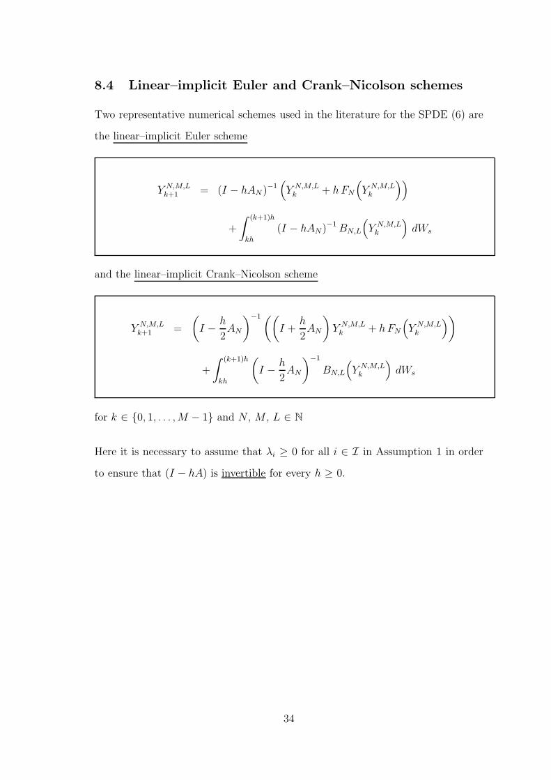
8.4 Linear–implicit Euler and Crank–Nicolson schemes
Two representative numerical schemes used in the literature for the SPDE (6) are
the linear–implicit Euler scheme
YN,M,L
k+1 = (I − hAN )−1(
YN,M,L
k + hFN
(
YN,M,L
k
))
+
∫ (k+1)h
kh
(I − hAN)−1BN,L
(
YN,M,L
k
)
dWs
and the linear–implicit Crank–Nicolson scheme
YN,M,L
k+1 =
(
I −h
2AN
)−1((
I +h
2AN
)
YN,M,L
k + hFN
(
YN,M,L
k
)
)
+
∫ (k+1)h
kh
(
I −h
2AN
)−1
BN,L
(
YN,M,L
k
)
dWs
for k ∈ 0, 1, . . . ,M − 1 and N , M , L ∈ N
Here it is necessary to assume that λi ≥ 0 for all i ∈ I in Assumption 1 in order
to ensure that (I − hA) is invertible for every h ≥ 0.
34

9 Global and local convergence orders
Taylor expansions provide a fundamental instrument for understanding the
local approximation properties of the solution of a differential equation.
For deterministic ODEs it is a general result (under suitable assumptions) that a
numerical scheme for an ODE has global convergence order p if it has local order
p+ 1 with p > 0.
Here local errors accumulate to give a larger global error.
For SODEs the situation is different.
A general result of Milstein that says that a numerical scheme for an
SODE with local order r > 12
has global convergence order r − 12.
The reason is that the errors in every step do not accumulate so rapidly since they
are centered and independent random variables. Hence usually a half order only is
lost.
35
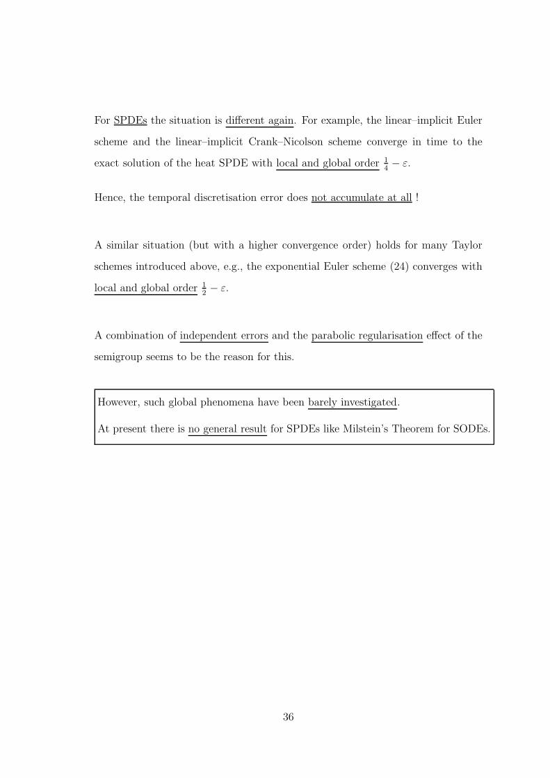
For SPDEs the situation is different again. For example, the linear–implicit Euler
scheme and the linear–implicit Crank–Nicolson scheme converge in time to the
exact solution of the heat SPDE with local and global order 14− ε.
Hence, the temporal discretisation error does not accumulate at all !
A similar situation (but with a higher convergence order) holds for many Taylor
schemes introduced above, e.g., the exponential Euler scheme (24) converges with
local and global order 12− ε.
A combination of independent errors and the parabolic regularisation effect of the
semigroup seems to be the reason for this.
However, such global phenomena have been barely investigated.
At present there is no general result for SPDEs like Milstein’s Theorem for SODEs.
36


![CBMS Innovation [Use of Handheld for Data Gathering] · 1 CBMS Innovation [Use of Handheld for Data Gathering] Province of Tarlac General Activities in Implementing CBMS Step 1 Advocacy](https://static.fdocuments.net/doc/165x107/5e2122c2dafdb9086b0ef648/cbms-innovation-use-of-handheld-for-data-gathering-1-cbms-innovation-use-of-handheld.jpg)