CAVITATION AND BUBBLE FORMATION IN WATER DISTRIBUTION SYSTEMS

Julia Ann Novak

Thesis submitted to the Faculty of the Virginia Polytechnic Institute and State University

in partial fulfillment of the requirements for the degree of

Master of Science in

Environmental Engineering

Dr. Marc Edwards, Chair Panayiotis Diplas G.V. Loganathan

April 8, 2005 Blacksburg, Virginia

Keywords: Gaseous Cavitation, Bubbles, Corrosion, Dissolved Gas

ii

Cavitation and Bubble Formation in Water Distribution Systems

Julia Novak

ABSTRACT Gaseous cavitation is examined from a practical and theoretical standpoint. Classical cavitation experiments which disregard dissolved gas are not directly relevant to natural water systems and require a redefined cavitation inception number which considers dissolved gases. In a pressurized water distribution system, classical cavitation is only expected to occur at extreme negative pressure caused by water hammer or at certain valves. Classical theory does not describe some practical phenomena including noisy pipes, necessity of air release valves, faulty instrument readings due to bubbles, and reports of premature pipe failure; inclusion of gaseous cavitation phenomena can better explain these events. Gaseous cavitation can be expected to influence corrosion in water distribution pipes. Bubbles can form within the water distribution system by a mechanism known as gaseous cavitation. A small scale apparatus was constructed to track gaseous cavitation as it could occur in buildings. Four independent measurements including visual observation of bubbles, an inline turbidimeter, an ultrasonic flow meter, and an inline total dissolved gas probe were used to track the phenomenon. All four measurements confirmed that gaseous cavitation was occurring within the experimental distribution system, even at pressures up to 40 psi. Gaseous cavitation was more likely at higher initial dissolved gas content, higher temperature, higher velocity and lower pressure. Certain changes in pH, conductivity, and surfactant concentration also tended to increase the likelihood of cavitation. For example, compared to the control at pH 5.0 and 30 psig, the turbidity increased 295% at pH 9.9. The formation of bubbles reduced the pump’s operating efficiency, and in the above example, the velocity was decreased by 17% at pH 9.9 versus pH 5.0.

iii

ACKNOWLEDGEMENTS

Thanks to my advisor, Marc Edwards, whose guidance, understanding and patience made this

thesis a reality. Thanks also to Paolo Scardina for providing me with a solid foundation in the understanding of

bubbles and saturation and for his help with paper structure and revisions. Thanks also to the Virginia Tech Via Fellowship, and to the Copper Development Association

and the National Science Foundation under grant DMI-0329474 for their funding of my graduate school program and research.

Finally, thanks to my devoted family and friends, whose support makes all of my accomplishments possible.

iv

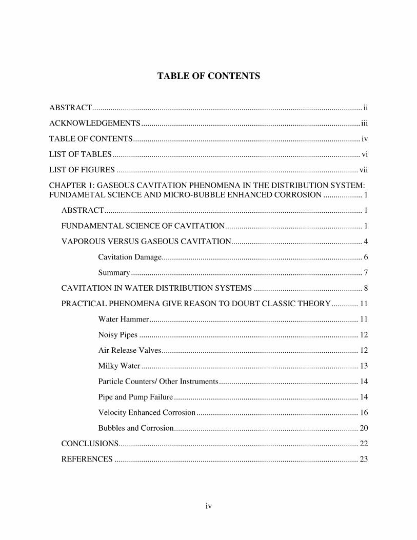
TABLE OF CONTENTS

ABSTRACT.................................................................................................................................... ii

ACKNOWLEDGEMENTS........................................................................................................... iii

TABLE OF CONTENTS............................................................................................................... iv

LIST OF TABLES......................................................................................................................... vi

LIST OF FIGURES ...................................................................................................................... vii

CHAPTER 1: GASEOUS CAVITATION PHENOMENA IN THE DISTRIBUTION SYSTEM: FUNDAMETAL SCIENCE AND MICRO-BUBBLE ENHANCED CORROSION ................... 1

ABSTRACT.............................................................................................................................. 1

FUNDAMENTAL SCIENCE OF CAVITATION................................................................... 1

VAPOROUS VERSUS GASEOUS CAVITATION................................................................ 4

Cavitation Damage.................................................................................................. 6

Summary................................................................................................................. 7

CAVITATION IN WATER DISTRIBUTION SYSTEMS ..................................................... 8

PRACTICAL PHENOMENA GIVE REASON TO DOUBT CLASSIC THEORY............. 11

Water Hammer...................................................................................................... 11

Noisy Pipes ........................................................................................................... 12

Air Release Valves................................................................................................ 12

Milky Water .......................................................................................................... 13

Particle Counters/ Other Instruments.................................................................... 14

Pipe and Pump Failure .......................................................................................... 14

Velocity Enhanced Corrosion ............................................................................... 16

Bubbles and Corrosion.......................................................................................... 20

CONCLUSIONS..................................................................................................................... 22

REFERENCES ....................................................................................................................... 23

v

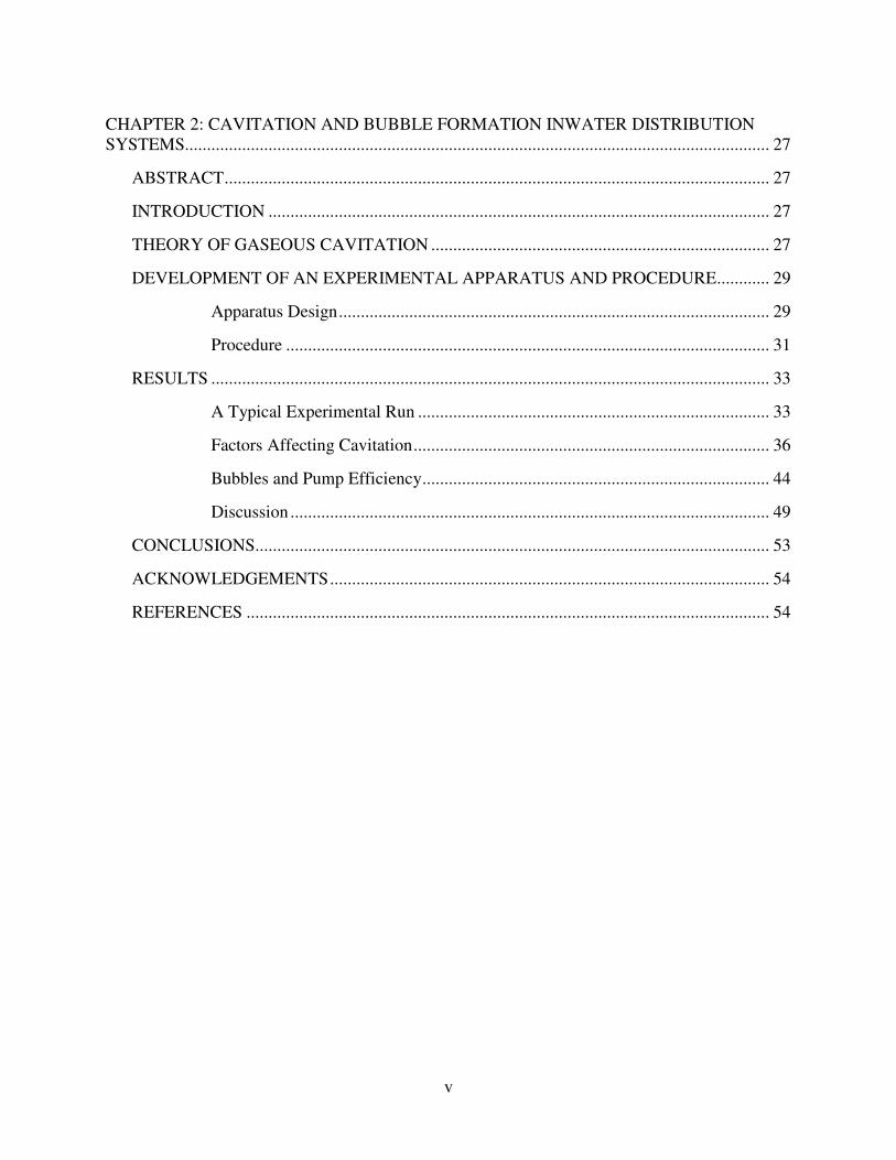
CHAPTER 2: CAVITATION AND BUBBLE FORMATION INWATER DISTRIBUTION SYSTEMS..................................................................................................................................... 27

ABSTRACT............................................................................................................................ 27

INTRODUCTION .................................................................................................................. 27

THEORY OF GASEOUS CAVITATION ............................................................................. 27

DEVELOPMENT OF AN EXPERIMENTAL APPARATUS AND PROCEDURE............ 29

Apparatus Design.................................................................................................. 29

Procedure .............................................................................................................. 31

RESULTS ............................................................................................................................... 33

A Typical Experimental Run ................................................................................ 33

Factors Affecting Cavitation................................................................................. 36

Bubbles and Pump Efficiency............................................................................... 44

Discussion ............................................................................................................. 49

CONCLUSIONS..................................................................................................................... 53

ACKNOWLEDGEMENTS.................................................................................................... 54

REFERENCES ....................................................................................................................... 54

vi

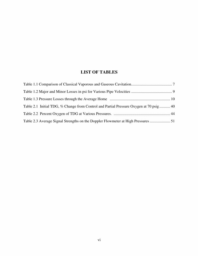
LIST OF TABLES

Table 1.1 Comparison of Classical Vaporous and Gaseous Cavitation.......................................... 7

Table 1.2 Major and Minor Losses in psi for Various Pipe Velocities .......................................... 9

Table 1.3 Pressure Losses through the Average Home .............................................................. 10

Table 2.1 Initial TDG, % Change from Control and Partial Pressure Oxygen at 70 psig ........... 40

Table 2.2 Percent Oxygen of TDG at Various Pressures. .......................................................... 44

Table 2.3 Average Signal Strengths on the Doppler Flowmeter at High Pressures ..................... 51

vii

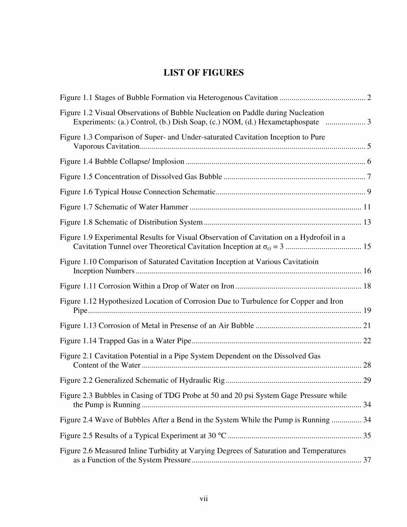
LIST OF FIGURES

Figure 1.1 Stages of Bubble Formation via Heterogenous Cavitation ........................................... 2

Figure 1.2 Visual Observations of Bubble Nucleation on Paddle during Nucleation Experiments: (a.) Control, (b.) Dish Soap, (c.) NOM, (d.) Hexametaphospate .................... 3

Figure 1.3 Comparison of Super- and Under-saturated Cavitation Inception to Pure Vaporous Cavitation................................................................................................................. 5

Figure 1.4 Bubble Collapse/ Implosion .......................................................................................... 6

Figure 1.5 Concentration of Dissolved Gas Bubble ....................................................................... 7

Figure 1.6 Typical House Connection Schematic........................................................................... 9

Figure 1.7 Schematic of Water Hammer ...................................................................................... 11

Figure 1.8 Schematic of Distribution System............................................................................... 13

Figure 1.9 Experimental Results for Visual Observation of Cavitation on a Hydrofoil in a Cavitation Tunnel over Theoretical Cavitation Inception at �ci = 3 ...................................... 15

Figure 1.10 Comparison of Saturated Cavitation Inception at Various Cavitatioin Inception Numbers ................................................................................................................. 16

Figure 1.11 Corrosion Within a Drop of Water on Iron ............................................................... 18

Figure 1.12 Hypothesized Location of Corrosion Due to Turbulence for Copper and Iron Pipe......................................................................................................................................... 19

Figure 1.13 Corrosion of Metal in Presense of an Air Bubble ..................................................... 21

Figure 1.14 Trapped Gas in a Water Pipe..................................................................................... 22

Figure 2.1 Cavitation Potential in a Pipe System Dependent on the Dissolved Gas Content of the Water .............................................................................................................. 28

Figure 2.2 Generalized Schematic of Hydraulic Rig .................................................................... 29

Figure 2.3 Bubbles in Casing of TDG Probe at 50 and 20 psi System Gage Pressure while the Pump is Running .............................................................................................................. 34

Figure 2.4 Wave of Bubbles After a Bend in the System While the Pump is Running ............... 34

Figure 2.5 Results of a Typical Experiment at 30 °C ................................................................... 35

Figure 2.6 Measured Inline Turbidity at Varying Degrees of Saturation and Temperatures as a Function of the System Pressure ..................................................................................... 37

viii

Figure 2.7 Cumulative Bubble Volumes at Varying Degrees of Saturation and Temperatures as a Function of the System Pressure .............................................................. 37

Figure 2.8 TDG Readings for Saturation/Temperature Experiments ........................................... 38

Figure 2.9 Measured Inline Turbidity as a Function of System Pressure of Various Water Qualities ................................................................................................................................. 41

Figure 2.10 Cumulative Bubble Volume as a Function of System Pressure of Various Water Qualities....................................................................................................................... 42

Figure 2.11 Cumulative Mass of Dissolved Gas as a Function of System Pressure of Selected Water Qualities ........................................................................................................ 43

Figure 2.12 Manufacturer's Pump Curve and Typical System Curves......................................... 45

Figure 2.13 Measured Velocity as a Function the System Pressures 50 psig and below; for Various Water Saturation Values at 30 and 45 degrees ................................................... 46

Figure 2.14 Measured Velocity as a Function the System Pressures 50 psig and below; All Water Qualities................................................................................................................. 47

Figure 2.15 Measured Velocity as a Function of Cumulative Bubble Volume of All Water Qualities for Pressures 50 psig and Lower............................................................................. 48

Figure 2.16 Measured Inline Turbidity as a Function of Calculated Bubble Volume of All Water Qualities....................................................................................................................... 50

Figure 2.17 Correlation of Signal Strength at 60 psig to 30 psig Turbidity and 20 psig Cumulative Bubble Volume for Every Experimental Run .................................................... 52

Figure 2.18 Diagram of a Septum in a 90-degree bend ................................................................ 53

- 1 -

Gaseous Cavitation Phenomena in the Distribution System: Fundamental Science and Micro-bubble Enhanced Corrosion

Julia Novak, Marc Edwards

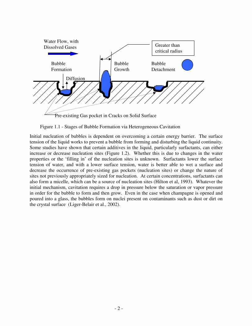
ABSTRACT. Gaseous cavitation is examined from a practical and theoretical standpoint. Classical cavitation experiments which disregard dissolved gas are not directly relevant to natural water systems and require a redefined cavitation inception number which considers dissolved gases. In a pressurized water distribution system, classical cavitation is only expected to occur at extreme negative pressure caused by water hammer or at certain valves. Classical theory does not describe some practical phenomena including noisy pipes, necessity of air release valves, faulty instrument readings due to bubbles, and reports of premature pipe failure; inclusion of gaseous cavitation phenomena can better explain these events. Gaseous cavitation can be expected to influence corrosion in water distribution pipes. FUNDAMENTAL SCIENCE OF CAVITATION. Cavitation is the process by which gas or vapor bubbles nucleate, grow, and then collapse in a liquid. Nucleation is the initial process by which bubbles form, and can occur in either a homogenous or heterogeneous manner. Homogeneous nucleation refers to the spontaneous formation of bubbles in the fluid, whereas heterogeneous nucleation occurs by growth of pre-existing gas nuclei present on particles suspended in the bulk solution and in cracks on solid surfaces. For water at normal temperatures, homogeneous nucleation is virtually irrelevant (Brennen, 1995; Liger-Belair, et al. 2002) due to the very high levels of supersaturation that are required. In heterogeneous nucleation (Figure 1.1), dissolved gas from the bulk liquid diffuses into a bubble forming in tiny cracks and irregularities on surfaces (Harvey, 1975). There may be very specific requirements for these nucleation cracks. To be a gas cavity, a very specific radius of curvature that is greater than a critical radius must exist (Liger-Belair et al., 2002). However, too large a crack will not permit surface tension to maintain an air pocket. Heterogeneous nucleation of bubbles along surfaces may be the precursor to suspended cavitation nuclei that allow for homogeneous nucleation.

- 2 -

Initial nucleation of bubbles is dependent on overcoming a certain energy barrier. The surface tension of the liquid works to prevent a bubble from forming and disturbing the liquid continuity. Some studies have shown that certain additives in the liquid, particularly surfactants, can either increase or decrease nucleation sites (Figure 1.2). Whether this is due to changes in the water properties or the ‘filling in’ of the nucleation sites is unknown. Surfactants lower the surface tension of water, and with a lower surface tension, water is better able to wet a surface and decrease the occurrence of pre-existing gas pockets (nucleation sites) or change the nature of sites not previously appropriately sized for nucleation. At certain concentrations, surfactants can also form a micelle, which can be a source of nucleation sites (Hilton et al, 1993). Whatever the initial mechanism, cavitation requires a drop in pressure below the saturation or vapor pressure in order for the bubble to form and then grow. Even in the case when champagne is opened and poured into a glass, the bubbles form on nuclei present on contaminants such as dust or dirt on the crystal surface (Liger-Belair et al., 2002).

Figure 1.1 - Stages of Bubble Formation via Heterogeneous Cavitation

Bubble Detachment

Diffusion

Bubble Growth

Bubble Formation

Water Flow, with Dissolved Gases

Pre-existing Gas pocket in Cracks on Solid Surface

Greater than critical radius

- 3 -

Figure 1.2 – Visual Observations of Bubble Nucleation on Paddle during Nucleation Experiments: (a.) Control, (b.) Dish Soap, (c.) NOM, (d.) Hexametaphosphate. (after Scardina et

al., 2004, b) Solutions Were Mixed at 40 rpm (G = 42 sec-1). Painting the Surface Could Smooth Surface Imperfections that

Cause Gas Bubble Nucleation or Could Make the Surface More Hydrophobic. Once nuclei are formed, if local pressure remains lower than the critical pressure, bubbles will increase in size, according to the generalized Rayleigh-Plesset equation for bubble dynamics including consideration for dissolved gases

R�

SdtdR

R�

dtdR

dtRd

RRR

TT

�

p�

)(T) - p(Tp

�

(t)) - p(TpL

LB

L

G

L

vBv

L

v 2423

2

2

2300 ++�

�

���

�+=��

���

���

���

�++∞

∞∞∞

(Equation 1.1) where pv is the vapor pressure in the bubble, pGo is the initial gas content of the bubble, TB is the temperature of the bubble, T� is the temperature far away from the bubble, pb is the pressure of the bubble, p� is the pressure far away from the bubble, �L is the density of the liquid, R is the radius of the bubble, �L is the kinematic viscosity of the liquid, and S is the surface tension. This equation allows for consideration of bubble pressure, ambient system pressure, mass diffusion effects and temperature effects for vaporous or gaseous bubbles. With a few basic assumptions of constant temperature and polytropic behavior of the bubble, the radius of a bubble can be determined at any given ambient system pressure and an assumed spherical bubble shape. Many times, however, bubbles are not spherical. More complicated models have been developed more recently to account for the instabilities of the oscillating spherical bubble, and the dynamics of nonspherical bubbles, but they are not empirically proven (Feng et al., 1997).

(a.)

(c.)

(b.)

(d.)

- 4 -

When the local pressure is higher than than the total dissolved gas pressure, the bubble will disappear, sometimes violently. The maximum pressure from the bubble collapse is estimated at tens of thousands of pounds per square inch (psi) and the timespan of collapse can be less than a millisecond (Konno et al., 2001). These implosions create “microjets” that can travel faster than the speed of sound and cause severe pitting in metal (Siegenthaler, 2000). Although theoretically this collapse occurs instantaneously after the bubble moves into an area of higher pressure, the bubbles can persist 20 times beyond the nozzle diameter in jet cavitation in tap water nearly saturated with dissolved gas even at pressures up to 72 psig (Nakano et al., 2001). It is possible that the dissolved gases present in the tap water increase the persistence of the bubbles. VAPOROUS VERSUS GASEOUS CAVITATION. Vaporous cavitation occurs when the bubble is comprised entirely of water vapor, due to local solution pressure dropping below the vapor pressure and “boiling” the water at ambient temperature. The cavitation inception number is defined as

2vfl

ci U0.5�p - p

� = (Equation 1.2)

where σci is the cavitation inception number, pfl is the fluid pressure, pv is the vapor pressure of the liquid at a given temperature, � is the fluid density and U is the free stream velocity. The cavitation inception number, σci, is a dimensionless number used to evaluate the potential for cavitation in a system. Typically cavitation becomes a significant problem when σci drops below 3, although the number has been known to vary depending on circumstances and the system. It has been noted that cavitation inception increases with higher dissolved gas contents (Brennen, 1993). When the nucleation bubble reaches a critical diameter, the bubble grows rapidly as long as the pressure is at or below the vapor pressure of the liquid. Cavitation occurs due to the presence of localized pressure drops in vortices which arise from turbulent eddies (Totten et al., 1998). Turbulent eddies can be formed in a water system at a sudden expansion, at bends and branchings, or at other appurtenances such as valves. Gaseous cavitation refers to bubbles comprised of dissolved gases and formed by a pressure drop below the saturation pressure of the constituent gases (pfl < pg). The distribution of gases in a water in equilibrium with the air are governed by Henry’s Law

kC pgas = (Equation 1.3)

at a constant temperature, where pgas is the partial pressure of the individual gas, k is Henry’s constant and C is the concentration of the gas in air. Henry’s Law states that the solubility of a dissolved gas is directly proportional to the pressure on the fluid. The total dissolved gas pressure is equal to the summation of the partial pressure plus the vapor pressure of water. Typical vapor pressures of water from 10-40° C range from 0.012 to 0.073 atmospheres, whereas the total dissolved gas pressure of natural water is typically in the range from 0.8 to 1.2 atmospheres (Scardina et al., 2004a). Decreasing the pressure to below the total dissolved gas pressure will tend to grow gas bubbles at nucleation sites. Gaseous cavitation bubbles are easily

- 5 -

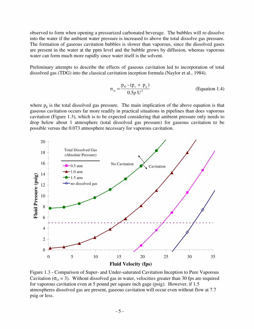
observed to form when opening a pressurized carbonated beverage. The bubbles will re-dissolve into the water if the ambient water pressure is increased to above the total dissolve gas pressure. The formation of gaseous cavitation bubbles is slower than vaporous, since the dissolved gases are present in the water at the ppm level and the bubble grows by diffusion, whereas vaporous water can form much more rapidly since water itself is the solvent. Preliminary attempts to describe the effects of gaseous cavitation led to incorporation of total dissolved gas (TDG) into the classical cavitation inception formula (Naylor et al., 1984).

2gvfl

ci U0.5�

)p (p - p �

+= (Equation 1.4)

where pg is the total dissolved gas pressure. The main implication of the above equation is that gaseous cavitation occurs far more readily in practical situations in pipelines than does vaporous cavitation (Figure 1.3), which is to be expected considering that ambient pressure only needs to drop below about 1 atmosphere (total dissolved gas pressure) for gaseous cavitation to be possible versus the 0.073 atmosphere necessary for vaporous cavitation.

0

2

4

6

8

10

12

14

16

18

20

0 5 10 15 20 25 30 35

Fluid Velocity (fps)

Flui

d Pr

essu

re (p

sig)

0.5 atm1.0 atm1.5 atmno dissolved gas

Total Dissolved Gas (Absolute Pressure)

No CavitationCavitation

Figure 1.3 - Comparison of Super- and Under-saturated Cavitation Inception to Pure Vaporous Cavitation (σci = 3). Without dissolved gas in water, velocities greater than 30 fps are required for vaporous cavitation even at 5 pound per square inch gage (psig). However, if 1.5 atmospheres dissolved gas are present, gaseous cavitation will occur even without flow at 7.7 psig or less.

- 6 -

Cavitation Damage Cavitation damage is generally thought to occur from the collapse of the cavitation bubbles (Figure 1.4). The microjets formed are extremely small and short-lived, but they are still very damaging; in some cases impacting metal surfaces with such force as to literally rip away minute amounts of metal (Siegenthaler, 2000). Although typical gas content is not considered in cavitation, Plesset and Prosperetti noted that some gas content in a vapor bubble could mitigate a violent collapse (Plesset and Prosperetti, 1977). More recently, it has been shown that the implosion of vaporous cavitation is not as violent if gases such as nitrogen were present in the bubble (Koivula, 2000). Additionally, the release of dissolved gases can also cause the damping of pressure waves following a cavitating flow (Kranenburg, 1974).

Gaseous cavitation is generally not attributed to great cavitation damage, but it is instead implicated in excessive system noise (Totten et al., 1998). However, research on the subject is limited. In fact, much of the research on vaporous cavitation was done in waters containing dissolved gas, in which case the observed damage is due to a combination of the two phenomena. The damage from gaseous cavitation may be due to indirect effects: the increased gas content in the bubble could serve as an oxygen reservoir for corrosion or bacterial growth. To illustrate, at higher pressures in a water distribution system, the partial pressure of oxygen in the compressed air, once it is released to solution is very high (Figure 1.5). If they do not implode but instead re-dissolve slowly the bubbles could collect in places along the pipe, for example in the rough surface of scale formation or bacterial plaque in the pipes. These spots could be prime spots for trapping highly oxygenated bubbles providing reactants for reduction reactions that drive corrosion. This could be a factor in localized corrosion.

Figure 1.4 - Bubble Collapse/ Implosion

Water Flow

Bubble collapse - directly on the pipe wall

Contraction to instigate cavitation

Bubble collapse – shock force impinges on wall

- 7 -

Summary Table 1.1 compares vaporous and gaseous cavitation. As long as the water contains dissolved gas, gaseous cavitation will always occur at higher pressure and lower velocity than vaporous cavitation. However, given the kinetic limitations to gas diffusion into growing bubbles, it might be that vaporous cavitation bubbles dominate in some circumstances. Bubble collapse and implosion pressures are often modified by the presence of other gases; if gas quantity is great, the slow nucleation of the cavity will produce less violent implosions (Koivula, 2000). In practice, all cavitation occurring in natural waters will be either gaseous cavitation, or at least a combination of gaseous and vaporous cavitation. This is interesting, because the presence and role of dissolved gases are often ignored in research done on the subject. Table 1.1: Comparison of Classical Vaporous and Gaseous Cavitation Parameter Vaporous Cavitation Gaseous Cavitation Bubble formation rate Very quick on the order of

thousandths of a second Bubbles grow more slowly due to diffusion from bulk solution

Bubble disappearance Vapor will condense in milliseconds once higher pressures are encountered

Bubbles disappear by dissolution of gases into the water (several seconds)

Implosion pressures extremely violent presence of dissolved gases smooths pressure spikes (Lai et al., 2000)

Typical gas content Almost entirely water vapor Nitrogen, oxygen, CO2, Cl2, Ar

Water Flow xygen

1) Cavitation Inception

10 mg/L Dissolved Oxygen

2) Bubble Growth

Figure 1.5 - Concentration of Dissolved Gas Bubble. Steps 1 and 2 occur during flow. Step 3 occurs after the valve is closed again.

3) Formation of Air Pocket, 4 atm pressure; 40 mg/L Oxygen in Bubble

System Pressure 60 psig

- 8 -

CAVITATION IN WATER DISTRIBUTION SYSTEMS. Cavitation is not generally considered to be a concern in water distribution systems, with the exception of pump stations. Calculations based on Bernoulli’s equations show that gaseous cavitation should not occur in pipes, given typical system pressures of 20 psi or greater (Figure 1.3). Even deliberate attempts to construct venturi suction devices in a water system have failed when pressure differentials were 40 to 60 psi (Cauton et al., 2000), since the local solution velocity cannot drop the pressure low enough. The basic equations defining energy losses during pipeline flow (Equation 1.5), minor head loss through appurtenances such as bends, tees, valves (Equation 1.6), and major friction losses through a pipe (Equation 1.7) have been defined:

z�

p2gV

z�

p2gV

21 22

22

11

21

� −+++=++ LH (Equation 1.5)

2gV 2

K (Equation 1.6)

86554

8521

8521

852110020830 .

.

.

.

LdQ

*C

*.h = (Equation 1.7)

Where V is the velocity in the pipe, and g is the gravitational constant, p is the pressure, � is the specific weight of water, z is the elevation head, HL is the head loss between points 1 and 2, K is the minor loss coefficient dependant on the type of appurtenance, hL is the head loss in feet per 100 feet of pipe, C is the Hazen-Williams flow factor dependent on the material and age of the pipe, Q is volumetric flow rate in gallons per minute, and d is the inside pipe diameter in inches. Both minor (US Corps of Engineers, 1999) and major losses increase with increasing pipe velocity (Table 1.2). An average 1500 square foot home typically has 20 ninety-degree bends, 10 tees, 2 reducers, and at least 4 valves (typically gate valves). Table 1.3 gives the total minor losses through all of these appurtenances and an assumed loss for one path of the house network (assume 3 tees, 5 bends, 2 contractions, and one valve). This hypothetical home is connected to a larger water distribution network via a tap into the main distribution system pipe (Figure 1.6). In the distribution system, pipe sizes are too large for significant friction loss, e.g. less than 1 psi every 50 feet for an 8-inch pipe at flows up to 8 fps (Table 1.2). Minor losses through bends, valves, and other appurtenances are not significant below 8 fps (Table 1.2).

- 9 -

Table 1.2: Major and Minor Losses in psi for Various Pipe Velocities

Average Water Velocity 2 fps 5 fps 8 fps 10 fps 15 fps 25 fps MAJOR LOSSES

0.5–inch diameter pipe 1.37 7.46 17.80 26.89 56.93 146.48 0.75–inch diameter pipe 0.85 4.65 11.09 16.75 35.47 91.26 1–inch diameter pipe 0.61 3.32 7.93 11.98 25.35 65.23 1.25–inch diameter pipe 0.47 2.56 6.11 9.23 19.54 50.28 2–inch diameter pipe 0.27 1.48 3.53 5.33 11.29 29.05 4–inch diameter pipe 0.12 0.66 1.57 2.38 5.03 12.94 8–inch diameter pipe 0.05 0.29 0.70 1.06 2.24 5.76 12–inch diameter pipe 0.03 0.18 0.44 0.66 1.40 3.59 16–inch diameter pipe 0.02 0.13 0.31 0.47 1.00 2.57

MINOR LOSSES Branch of Tee 0.05 0.30 0.77 1.21 2.72 7.56 90-degree Bend 0.02 0.15 0.39 0.60 1.36 3.78 Contraction 0.02 0.10 0.26 0.40 0.91 2.52 Gate Valve, fully open 0.01 0.03 0.09 0.13 0.30 0.84

Note: Major loss for 50 foot of pipe, C = 120

Figure 1.6 - Typical House Connection Schematic

Distribution System

Setback

House typical ¾ inch copper piping

Property Line

Tapping into water main

Typically 6-inch to 12-inch mains

W Typical 2-inch or smaller water line

Water Meter

- 10 -

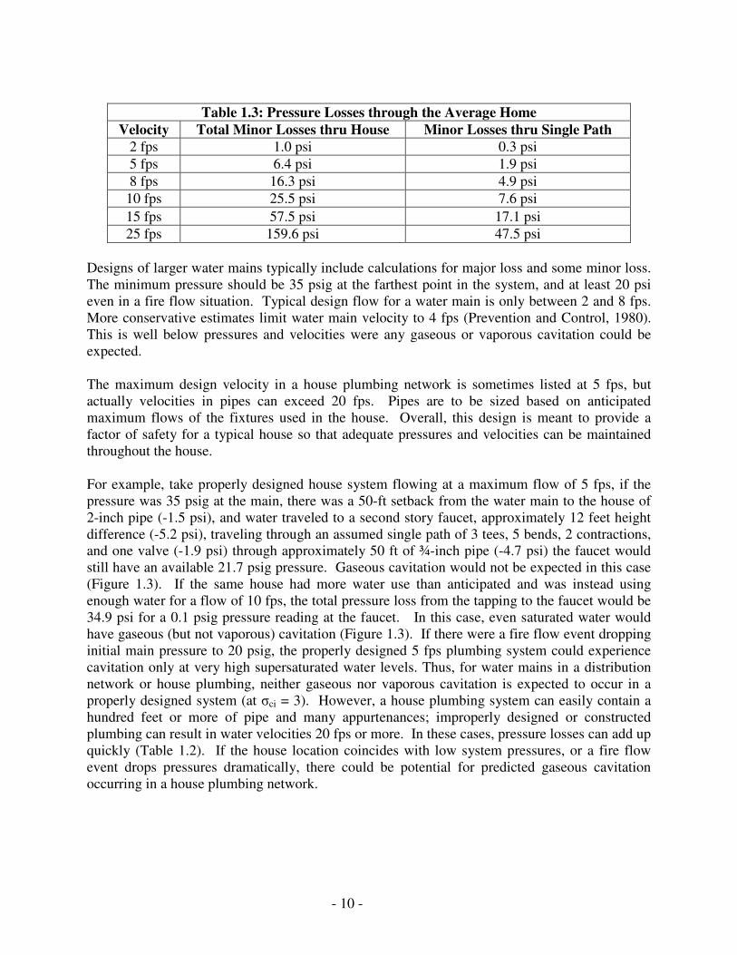
Table 1.3: Pressure Losses through the Average Home

Velocity Total Minor Losses thru House Minor Losses thru Single Path 2 fps 1.0 psi 0.3 psi 5 fps 6.4 psi 1.9 psi 8 fps 16.3 psi 4.9 psi

10 fps 25.5 psi 7.6 psi 15 fps 57.5 psi 17.1 psi 25 fps 159.6 psi 47.5 psi

Designs of larger water mains typically include calculations for major loss and some minor loss. The minimum pressure should be 35 psig at the farthest point in the system, and at least 20 psi even in a fire flow situation. Typical design flow for a water main is only between 2 and 8 fps. More conservative estimates limit water main velocity to 4 fps (Prevention and Control, 1980). This is well below pressures and velocities were any gaseous or vaporous cavitation could be expected. The maximum design velocity in a house plumbing network is sometimes listed at 5 fps, but actually velocities in pipes can exceed 20 fps. Pipes are to be sized based on anticipated maximum flows of the fixtures used in the house. Overall, this design is meant to provide a factor of safety for a typical house so that adequate pressures and velocities can be maintained throughout the house. For example, take properly designed house system flowing at a maximum flow of 5 fps, if the pressure was 35 psig at the main, there was a 50-ft setback from the water main to the house of 2-inch pipe (-1.5 psi), and water traveled to a second story faucet, approximately 12 feet height difference (-5.2 psi), traveling through an assumed single path of 3 tees, 5 bends, 2 contractions, and one valve (-1.9 psi) through approximately 50 ft of ¾-inch pipe (-4.7 psi) the faucet would still have an available 21.7 psig pressure. Gaseous cavitation would not be expected in this case (Figure 1.3). If the same house had more water use than anticipated and was instead using enough water for a flow of 10 fps, the total pressure loss from the tapping to the faucet would be 34.9 psi for a 0.1 psig pressure reading at the faucet. In this case, even saturated water would have gaseous (but not vaporous) cavitation (Figure 1.3). If there were a fire flow event dropping initial main pressure to 20 psig, the properly designed 5 fps plumbing system could experience cavitation only at very high supersaturated water levels. Thus, for water mains in a distribution network or house plumbing, neither gaseous nor vaporous cavitation is expected to occur in a properly designed system (at �ci = 3). However, a house plumbing system can easily contain a hundred feet or more of pipe and many appurtenances; improperly designed or constructed plumbing can result in water velocities 20 fps or more. In these cases, pressure losses can add up quickly (Table 1.2). If the house location coincides with low system pressures, or a fire flow event drops pressures dramatically, there could be potential for predicted gaseous cavitation occurring in a house plumbing network.

- 11 -

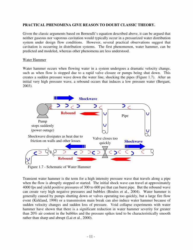
PRACTICAL PHENOMENA GIVE REASON TO DOUBT CLASSIC THEORY. Given the classic arguments based on Bernoulli’s equation described above, it can be argued that neither gaseous nor vaporous cavitation would typically occur in a pressurized water distribution system under design flow conditions. However, several practical observations suggest that cavitation is occurring in distribution systems. The first phenomenon, water hammer, can be predicted and modeled, whereas other phenomena are less understood. Water Hammer Water hammer occurs when flowing water in a system undergoes a dramatic velocity change, such as when flow is stopped due to a rapid valve closure or pumps being shut down. This creates a sudden pressure wave down the water line, shocking the pipes (Figure 1.7). After an initial very high pressure wave, a rebound occurs that induces a low pressure water (Bergant, 2003).

Transient water hammer is the term for a high intensity pressure wave that travels along a pipe when the flow is abruptly stopped or started. The initial shock wave can travel at approximately 4000 fps and yield positive pressures of 300 to 600 psi that can burst pipe. But the rebound wave can create very high negative pressures and bubbles (Boulos et al., 2004). Water hammer is generally caused by pumps shutting down or valves operating too quickly, but a large fire flow event (Kirkland, 1998) or a transmission main break can also induce water hammer because of sudden velocity changes and sudden loss of pressure. Void collapse experiments with water hammer have shown that there is a significant reduction in water hammer severity for greater than 20% air content in the bubbles and the pressure spikes tend to be characteristically smooth rather than sharp and abrupt (Lai et al., 2000).

Figure 1.7 - Schematic of Water Hammer

Pipe Pump

stops suddenly (power outage)

Shockwave

Shockwave dissipates as heat due to friction on walls and other losses

Valve closes too quickly

Rebound

Shockwave

Rebound

- 12 -

Additionally, vaporous cavitation can occur at the very high velocities present within a partly closed valve (Lahlou, 2002). Negative pressures from pressure transients are significant enough to allow water that is surrounding the pipe to be drawn into the distribution system (Boyd et al., 2004). These pressure transients have only a short duration and can go undetected; but incidents of intrusion into a pressurized distribution system may be more common that previously thought (LeChevallier et al., 2003). There is currently no evidence or discussion of intrusion events occurring in home plumbing. Noisy Pipes Bubble formation in pipes can result in significant noise. It is believed that continuous noise from pipes can come from bubbles forming at bends. A crackling or popping sound is often the first indication in pumps that cavitation could be occurring. The frequency of the noise depends on a variety of factors including the size of the bubbles and the speed of the flow. Because most water systems are buried, any noise wouldn’t be evident but noise from pipes in homes can be heard by residents. The amount of noise can vary depending on the time of year (i.e. water temperature) and the velocity of the water in the pipes. The sound of water in pipes increases with dissolved gases (Stryker, 2003), and according to popular advice given to homeowners, pump noise can be stopped completely by appropriate adjustments of pressure, velocity or dissolved gas content (Siegenthaler, 2000). Air Release Valves The placement of air release valves is generally based on AWWA recommendations developed with empirical evidence and common sense regarding portions of pipelines in which air is likely to accumulate. Automatic valves have been developed since it is unknown how much air accumulates over what time period. Their sizing and design is often based on a worst case scenario, in which is it assumed since water is 2% air, that amount should be used for the nominal venting capacity (Equation 1.8).

q = Q * (0.13 cu ft/gal) * .02 Equation (1.8) where q is the air flow and Q is the system flow rate (gpm) (Air Valve, 1996). This is obviously in direct conflict with the earlier theory for flow in a water main. Even with these conservative AWWA guidelines, insufficient air-release valves are installed, resulting in gas buildup that can greatly reduce flow (Kirkland, 1998). The amount of air released is unknown, but without air release valves, the air can cause significant decrease in effective pipe diameter, increasing the actual water velocity in the pipe (exacerbating the problem) and head loss, or even causing air binding and stopping flow entirely (Karassik et al., 2001). The introduction of air into pipelines is attributed to a variety of causes including forced entrainment by pumps, low pressure zones created by change in pipe diameter, slope and elevation, partially filled pipes, or opened and leaky valves (AWWA, 2001). It is also noted that air can enter through leaky joints where suction exists, but this is suggested to only occur near pumps or in locations where the pipeline is above the hydraulic grade line (HGL). While it is not ideal, in practice water mains can be buried above the HGL due to topography and cost

- 13 -

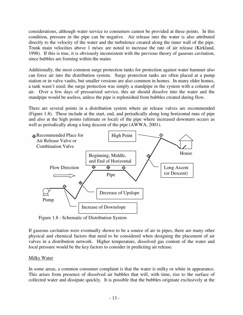
considerations, although water service to consumers cannot be provided at these points. In this condition, pressure in the pipe can be negative. Air release into the water is also attributed directly to the velocity of the water and the turbulence created along the inner wall of the pipe. Trunk main velocities above 1 m/sec are noted to increase the rate of air release (Kirkland, 1998). If this is true, it is obviously inconsistent with the previous theory of gaseous cavitation, since bubbles are forming within the mains Additionally, the most common surge protection tanks for protection against water hammer also can force air into the distribution system. Surge protection tanks are often placed at a pump station or in valve vaults, but smaller versions are also common in homes. In many older homes, a tank wasn’t used; the surge protection was simply a standpipe in the system with a column of air. Over a few days of pressurized service, this air should dissolve into the water and the standpipe would be useless, unless the pipe is replenished from bubbles created during flow. There are several points in a distribution system where air release valves are recommended (Figure 1.8). These include at the start, end, and periodically along long horizontal runs of pipe and also at the high points (ultimate or local) of the pipe where increased downturn occurs as well as periodically along a long descent of the pipe (AWWA, 2001).

If gaseous cavitation were eventually shown to be a source of air in pipes, there are many other physical and chemical factors that need to be considered when designing the placement of air valves in a distribution network. Higher temperature, dissolved gas content of the water and local pressure would be the key factors to consider in predicting air release. Milky Water In some areas, a common consumer complaint is that the water is milky or white in appearance. This arises from presence of dissolved air bubbles that will, with time, rise to the surface of collected water and dissipate quickly. It is possible that the bubbles originate exclusively at the

Figure 1.8 - Schematic of Distribution System

Pipe

Pump

Flow Direction

Recommended Place for Air Release Valve or Combination Valve

Increase of Downslope

Decrease of Upslope

Beginning, Middle, and End of Horizontal

High Point

Long Ascent (or Descent)

House

- 14 -

faucet aerator, but that the problem is exacerbated by dissolved gas pressure and temperature. This would explain the seasonal variation in such complaints. The pressure of dissolved gas in water varies seasonally and even daily due to factors such as algae growth in the source water (Scardina et al., 2002). It has also been reported that milky water problems are greater in newer pipes or near reservoirs, and removal of oxygen from the water by metal corrosion is thought to decrease the likelihood of the problem. Particle Counters/Other Instruments Particle counters are often used in water treatment plants to monitor filter performance. Many detectors claim accuracy in counting various sized particles from 2 to 400 microns in size, which could include pathogens. However, particles counters do not reliably distinguish between actual particles and bubbles. Indeed, the same light scattering techniques used for particle counts and size distribution determination can be used for bubbles. While many particle counters attempt to remove bubbles from the water, equipment manufacturers do not have supporting data to demonstrate that these bubble traps work effectively. A recent paper indicated that these traps do not function very effectively, and that bubbles interfere with particle counting in a manner consistent with gaseous cavitation in the flow cell (Scardina et al., 2004b). An ultrasonic flowmeter uses Doppler technology to bounce sound off moving turbidity or bubbles to measure velocity in a water system. These devices can function by placement on the external pipe wall without destructively altering the pipe. Manufacturer’s specifications for such devices state that, if the water has insufficient particles, placement of the monitor after a bend will allow the system to operate. Gaseous cavitation is the most likely explanation for bubble formation at bends, and indeed it may be a requirement for the device to measure flow. Pipe and Pump Failure Pump, valve and pipe failures are often attributed to cavitation. As mentioned previously, if velocity in water mains is between 2 and 8 fps, neither vaporous nor gaseous cavitation should occur (Figure 1.3). The local velocity can vary significantly from idealized flow defined by the classic Bernoulli’s equation (Equation 1.5), and it is understood that in microeddies pressures might be much lower than predicted (Birkhoff, 1957). The net result is that gaseous cavitation might be occurring in situations where Bernoulli’s equation predicts it would not. Once again, reports in the literature suggest that cavitation is occurring in pipes and that bubbles are contributing to failures. For example, Chan et al. (2002) report that many copper tube failures are occurring in buildings due to cavitation, but that velocity does not approach the 30 fps required for classic vaporous cavitation to occur. Similarly, attack on copper tube has been reported to worsen at higher dissolved gas content, which would be consistent with the increased likelihood of gaseous cavitation in Figure 1.3 (Knutsson et al., 1972). Temperature gradients may also be a factor in pipe failure. For drastic temperature changes, such as in a cooling water line in nuclear power plants, combined gas and liquid flows can develop and form cavitation bubbles (Giese et al., 2000).

- 15 -

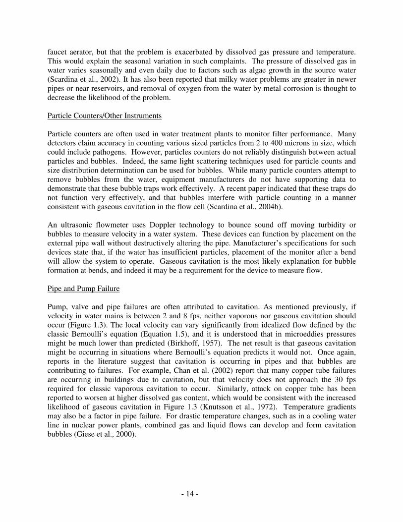
These practical observations suggest that gas is probably being created in more situations in the distribution system (Corcos, 2004). Thus, strict calculations may not completely describe the origins of the problem, and an improved theory may be needed. Hydrofoil work by Naylor and Millard demonstrate that while empirical values of cavitation inception are still applicable (Naylor et al., 1984), the dissolved gases are significant enough that they must be included in the calculation (Equation 1.4). The experimental values of visible cavitation occurrence matched very well with theoretical cavitation inception results when dissolved gases are included in the calculations (Figure 1.9). Note that while this hydrofoil experiment had velocities seen in distribution systems, it was conducted under vacuum conditions. However, the formula can be extended to pressures and gas contents expected in a distributions system, eg. 0.8, 1.0, and 1.2 atm. Cavitation is anticipated in regions below each line. It is possible that cavitation inception occurs at a higher characteristic number for gaseous cavitation when it occurs in pipelines (Figure 1.10). The main conclusion is that even based on Naylor and Millard's results, if the total dissolved gas content of the water is below 1.2 atmospheres, gaseous cavitation is not expected below 8 ft/sec even if local solution pressure dropped to 5 psi.

-20

-15

-10

-5

0

5

10

15

20

25

30

35

0 1 2 3 4 5 6 7 8 9 10

Fluid Velocity (fps)

Flui

d Pr

essu

re (p

sig)

.61 atm .61 atm 0.8 atm

.35 atm .35 atm 1.0 atm

.21 atm .21 atm 1.2 atm

.15 atm .15 atm

Total Dissolved Gas, Absolute Pressure

Theoretical Cavitation Inception

ExperimentalData

Typical House Velocity 5 fps

Minimum 2 fps Maximum 8 fpsTypical System Design Flow Range

Theoretical Cavitation Inception

Figure 1.9 - Experimental Results for Visual Observation of Cavitation on a Hydrofoil in a Cavitation Tunnel over Theoretical Cavitation Inception at a �ci = 3 (after Naylor et al., 1984)

- 16 -

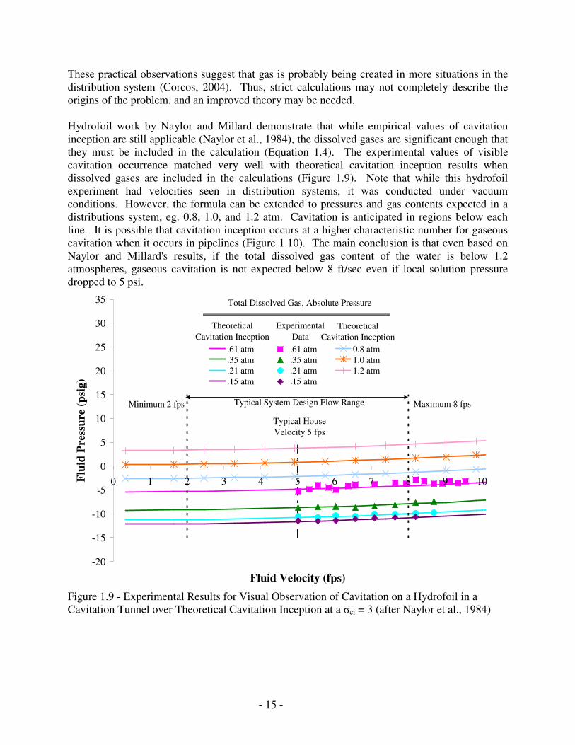
0

5

10

15

20

25

30

0 5 10 15 20 25 30 35

Fluid Velocity (fps)

Flui

d Pr

essu

re (p

sig)

1

2

3

4

5

Cavitation Inception Number for 1 atm Dissolved Gas

No Cavitation

Cavitation

Figure 1.10 - Comparison of Saturated Cavitation Inception at Various Cavitation Inception Numbers. Regions below each line indicate where cavitation may occur; a higher cavitation number would occur if cavitation was more likely than currently predicted, whereas a lower number indicates it is less likely. Velocity Enhanced Corrosion Corrosion influenced by the velocity of the fluid flowing through the piping system and is called flow-accelerated corrosion or flow assisted corrosion (Canadian C&B Devel. Assoc., Silbert, 2002), as evidenced by research on the relationship between copper tube wall thinning and pipe velocity published 45 years ago (Obrecht and Quill, 1960a-f; Obrecht and Quill, 1961; Obrecht et al., 1960). It is uncertain whether the adverse effects of higher velocity are due to enhanced diffusion of oxidants to the surface, enhanced removal of reaction products from the surface, mechanical shearing of protective corrosion scales from the pipe, or other issues such as bubble formation. This section describes a range of possible physical and chemical impacts of velocity on aspects of pipe corrosion.

- 17 -

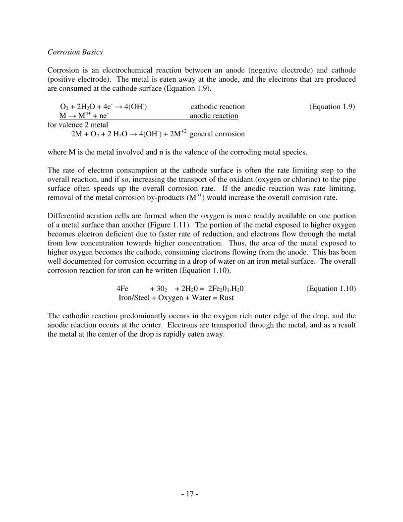
Corrosion Basics Corrosion is an electrochemical reaction between an anode (negative electrode) and cathode (positive electrode). The metal is eaten away at the anode, and the electrons that are produced are consumed at the cathode surface (Equation 1.9).

O2 + 2H2O + 4e- � 4(OH-) cathodic reaction (Equation 1.9) M � Mn+ + ne- anodic reaction

for valence 2 metal 2M + O2 + 2 H2O � 4(OH-) + 2M+2 general corrosion

where M is the metal involved and n is the valence of the corroding metal species. The rate of electron consumption at the cathode surface is often the rate limiting step to the overall reaction, and if so, increasing the transport of the oxidant (oxygen or chlorine) to the pipe surface often speeds up the overall corrosion rate. If the anodic reaction was rate limiting, removal of the metal corrosion by-products (Mn+) would increase the overall corrosion rate. Differential aeration cells are formed when the oxygen is more readily available on one portion of a metal surface than another (Figure 1.11). The portion of the metal exposed to higher oxygen becomes electron deficient due to faster rate of reduction, and electrons flow through the metal from low concentration towards higher concentration. Thus, the area of the metal exposed to higher oxygen becomes the cathode, consuming electrons flowing from the anode. This has been well documented for corrosion occurring in a drop of water on an iron metal surface. The overall corrosion reaction for iron can be written (Equation 1.10).

4Fe + 302 + 2H20 = 2Fe203.H20 (Equation 1.10) Iron/Steel + Oxygen + Water = Rust

The cathodic reaction predominantly occurs in the oxygen rich outer edge of the drop, and the anodic reaction occurs at the center. Electrons are transported through the metal, and as a result the metal at the center of the drop is rapidly eaten away.

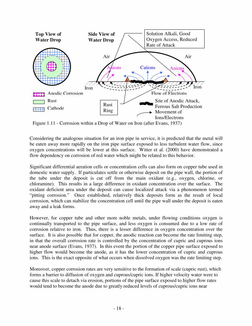
- 18 -

Considering the analogous situation for an iron pipe in service, it is predicted that the metal will be eaten away more rapidly on the iron pipe surface exposed to less turbulent water flow, since oxygen concentrations will be lower at this surface. Witter et al. (2000) have demonstrated a flow dependency on corrosion of red water which might be related to this behavior. Significant differential aeration cells or concentration cells can also form on copper tube used in domestic water supply. If particulates settle or otherwise deposit on the pipe wall, the portion of the tube under the deposit is cut off from the main oxidant (e.g., oxygen, chlorine, or chloramine). This results in a large difference in oxidant concentration over the surface. The oxidant deficient area under the deposit can cause localized attack via a phenomenon termed “pitting corrosion.” Once established, relatively thick deposits form as the result of local corrosion, which can stabilize the concentration cell until the pipe wall under the deposit is eaten away and a leak forms. However, for copper tube and other more noble metals, under flowing conditions oxygen is continually transported to the pipe surface, and less oxygen is consumed due to a low rate of corrosion relative to iron. Thus, there is a lesser difference in oxygen concentration over the surface. It is also possible that for copper, the anodic reaction can become the rate limiting step, in that the overall corrosion rate is controlled by the concentration of cupric and cuprous ions near anode surface (Evans, 1937). In this event the portion of the copper pipe surface exposed to higher flow would become the anode, as it has the lower concentration of cupric and cuprous ions. This is the exact opposite of what occurs when dissolved oxygen was the rate limiting step. Moreover, copper corrosion rates are very sensitive to the formation of scale (cupric rust), which forms a barrier to diffusion of oxygen and cuprous/cupric ions. If higher velocity water were to cause this scale to detach via erosion, portions of the pipe surface exposed to higher flow rates would tend to become the anode due to greatly reduced levels of cuprous/cupric ions near

Top View of Water Drop

Side View of Water Drop

Anodic Corrosion Rust Cathode

Cations

Air

Anions Anions

Flow of Electrons Iron

Solution Alkali, Good Oxygen Access, Reduced Rate of Attack

Rust Ring

Figure 1.11 - Corrosion within a Drop of Water on Iron (after Evans, 1937)

Movement of Ions/Electrons

Site of Anodic Attack, Ferrous Salt Production

Iron

Air

- 19 -

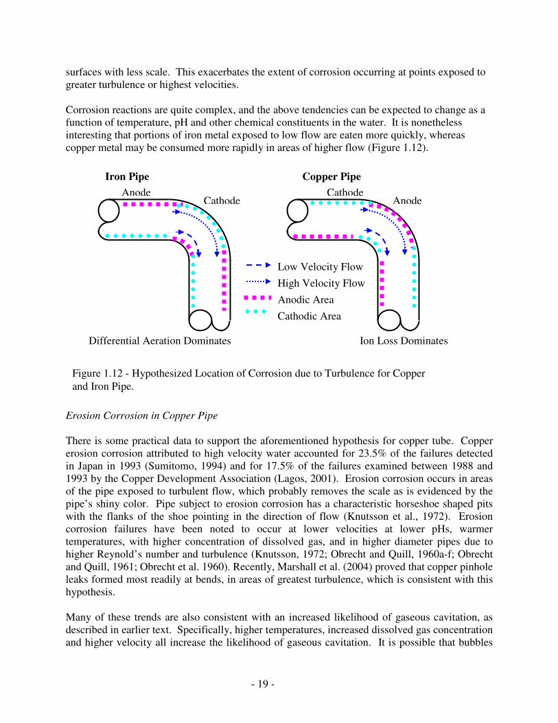
surfaces with less scale. This exacerbates the extent of corrosion occurring at points exposed to greater turbulence or highest velocities. Corrosion reactions are quite complex, and the above tendencies can be expected to change as a function of temperature, pH and other chemical constituents in the water. It is nonetheless interesting that portions of iron metal exposed to low flow are eaten more quickly, whereas copper metal may be consumed more rapidly in areas of higher flow (Figure 1.12).

Erosion Corrosion in Copper Pipe There is some practical data to support the aforementioned hypothesis for copper tube. Copper erosion corrosion attributed to high velocity water accounted for 23.5% of the failures detected in Japan in 1993 (Sumitomo, 1994) and for 17.5% of the failures examined between 1988 and 1993 by the Copper Development Association (Lagos, 2001). Erosion corrosion occurs in areas of the pipe exposed to turbulent flow, which probably removes the scale as is evidenced by the pipe’s shiny color. Pipe subject to erosion corrosion has a characteristic horseshoe shaped pits with the flanks of the shoe pointing in the direction of flow (Knutsson et al., 1972). Erosion corrosion failures have been noted to occur at lower velocities at lower pHs, warmer temperatures, with higher concentration of dissolved gas, and in higher diameter pipes due to higher Reynold’s number and turbulence (Knutsson, 1972; Obrecht and Quill, 1960a-f; Obrecht and Quill, 1961; Obrecht et al. 1960). Recently, Marshall et al. (2004) proved that copper pinhole leaks formed most readily at bends, in areas of greatest turbulence, which is consistent with this hypothesis. Many of these trends are also consistent with an increased likelihood of gaseous cavitation, as described in earlier text. Specifically, higher temperatures, increased dissolved gas concentration and higher velocity all increase the likelihood of gaseous cavitation. It is possible that bubbles

Figure 1.12 - Hypothesized Location of Corrosion due to Turbulence for Copper and Iron Pipe.

Iron Pipe Copper Pipe

Differential Aeration Dominates Ion Loss Dominates

Low Velocity Flow High Velocity Flow

Anode Cathode

Cathode Anode

Anodic Area Cathodic Area

- 20 -

are forming at bends during pipe flow, increasing detachment of scale and contributing to accelerated localized attack on copper. Indeed, a recent research paper identified “cavitation” as a major cause of copper tube failure in Hong Kong (Chan et al., 2002), but noted that vaporous cavitation should not be occurring in domestic water supplies. Gaseous cavitation may be the actual cause of pipe failure in these circumstances. In addition to chemistry, temperature and flow velocity changes, erosion corrosion also encompasses the mechanical destruction of the metal’s protective film by particulates (USACE, 1995). The impingement of particles on pipe surfaces at high velocities can remove protective scale and the metal itself. Corrosion product fines, sand and silt are all noted to increase corrosion rates (CNSC, 2003). Bubbles and Corrosion Bubbles can have a significant role in enhancing corrosion via gas bubble impingement, bubble implosion from vaporous cavitation, and trapped gas. Bubble Impingement For either iron or copper, direct contact of bubbles on a pipe wall can result in loss of pipe material or, more importantly, deterioration of protective films that have developed on the pipe. Entrained gases are known to increase corrosion rates and decrease the velocity at which cavitation occurs (Obrecht et al.,1960; Lagos, 2001). Bubbles traveling in a continuous cloud could have a scouring effect on the metal and could damage it significantly by erosion even without implosion of the bubbles or air trapping. Air scouring – the deliberate injection of air to scour and clean distribution pipes, is a recognized practical application of this idea (Severn Trent Services). The precise role of higher velocity, bubble size and concentration has not been evaluated experimentally. Implosion Bubble collapse after vaporous cavitation can occur with tremendous force and seriously damage metal due to creation of a shock wave (Figure 1.4). While pure vaporous cavitation probably does not occur in a water system saturated with dissolve gases, it is generally more damaging because of the forces involved and localized nature of the problem. Since dissolved gases cushion these implosions, damage from vaporous cavitation would be expected to decrease with higher gas content (Jang et al., 2003), as opposed to the tendency that is actually observed in practice. Trapped Gas Bubbles that have formed may not travel along with the water flow but instead cling to the metallic surface of pipe (Evans, 1937). In this case, corrosion would occur just outside of the air bubble (Figure 1.13). A bubble of air at atmospheric pressure would not be of much concern. The bubble would have its oxygen gradually removed (Evans, 1937), and the local concentration of dissolved oxygen would have started at only 8.4 mg/L at 25° C.

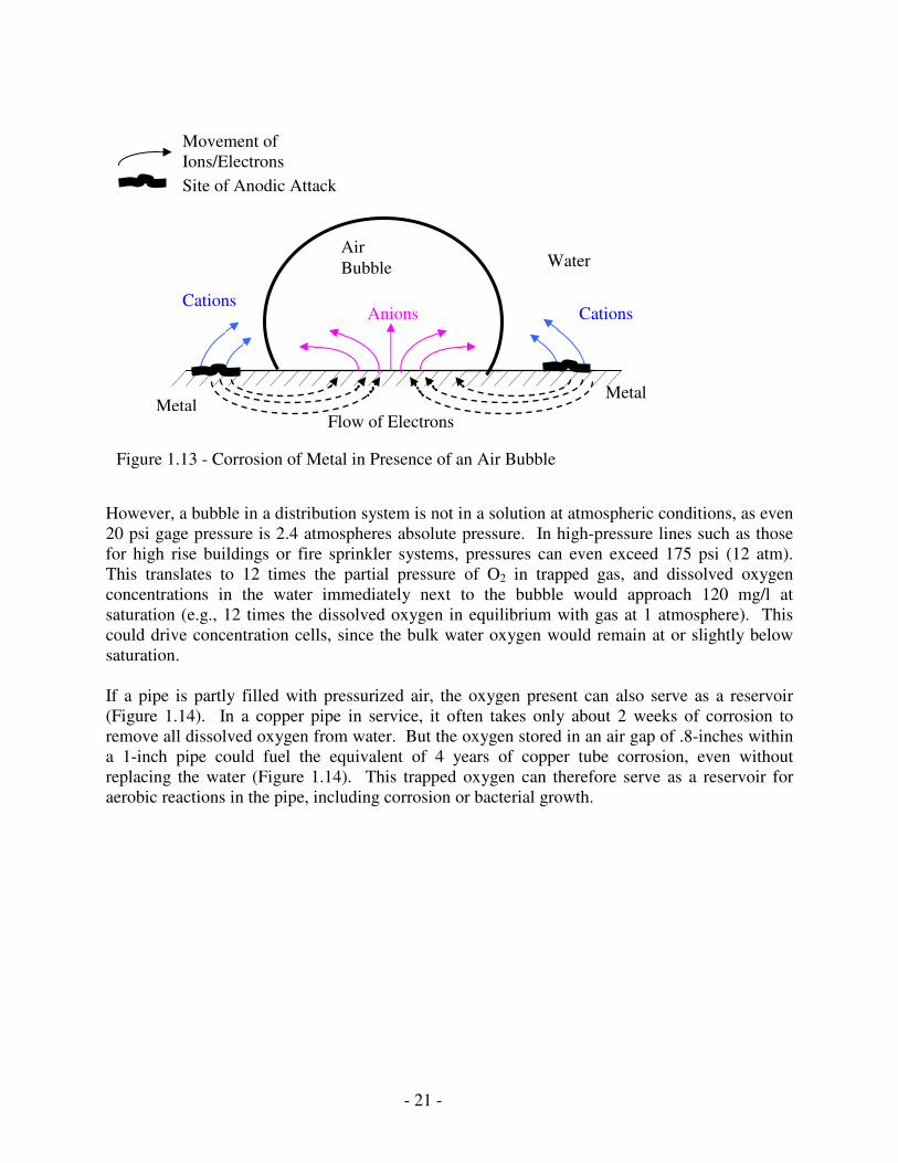
- 21 -

However, a bubble in a distribution system is not in a solution at atmospheric conditions, as even 20 psi gage pressure is 2.4 atmospheres absolute pressure. In high-pressure lines such as those for high rise buildings or fire sprinkler systems, pressures can even exceed 175 psi (12 atm). This translates to 12 times the partial pressure of O2 in trapped gas, and dissolved oxygen concentrations in the water immediately next to the bubble would approach 120 mg/l at saturation (e.g., 12 times the dissolved oxygen in equilibrium with gas at 1 atmosphere). This could drive concentration cells, since the bulk water oxygen would remain at or slightly below saturation. If a pipe is partly filled with pressurized air, the oxygen present can also serve as a reservoir (Figure 1.14). In a copper pipe in service, it often takes only about 2 weeks of corrosion to remove all dissolved oxygen from water. But the oxygen stored in an air gap of .8-inches within a 1-inch pipe could fuel the equivalent of 4 years of copper tube corrosion, even without replacing the water (Figure 1.14). This trapped oxygen can therefore serve as a reservoir for aerobic reactions in the pipe, including corrosion or bacterial growth.

Flow of Electrons Metal

Figure 1.13 - Corrosion of Metal in Presence of an Air Bubble

Site of Anodic Attack

Cations

Water

Anions

Metal

Air Bubble

Movement of Ions/Electrons

Cations

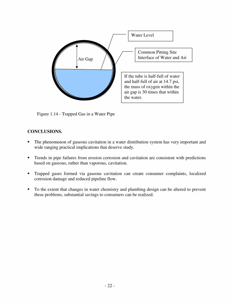
- 22 -

CONCLUSIONS. � The phenomenon of gaseous cavitation in a water distribution system has very important and

wide ranging practical implications that deserve study. � Trends in pipe failures from erosion corrosion and cavitation are consistent with predictions

based on gaseous, rather than vaporous, cavitation. � Trapped gases formed via gaseous cavitation can create consumer complaints, localized

corrosion damage and reduced pipeline flow. � To the extent that changes in water chemistry and plumbing design can be altered to prevent

these problems, substantial savings to consumers can be realized.

Figure 1.14 - Trapped Gas in a Water Pipe

If the tube is half-full of water and half-full of air at 14.7 psi, the mass of oxygen within the air gap is 30 times that within the water.

Air Gap

Water Level

Common Pitting Site Interface of Water and Air

- 23 -

REFERENCES. American Water Works Association. Air-Release, Air/Vacuum, & Combination Air Valves Manual of Water

Supply Practices American Water Works Association AWWA Manual M51, 2001. Bergant, Anton and Tijsseling, Arris (2003). “Parameters Affecting Water Hammer Wave Attenuation, Shape and

Timing”. Eindhoven University of Technology, The Netherlands. Birkhoff, G., Jets, Wakes, and Cavities. Academic Press, Inc., New York, 1957. Boulos, P.F., Lansey, K.E, and Karney, B.W. (2004) Comprehensive Water Distribution Systems Analysis

Handbook for Engineers and Planners. Pasadena, CA: MWH Soft. Pub. Boyd, Glen R., Wang, Hua, Britton, Michael D., Howie, Douglas C., Wood, Don J., Funk, James E., and Friedman

Melinda J. (2004). “Intrusion within a Simulated Water Distribution System due to Hydraulic Transients. I: Description of Test Rig and Chemical Tracer Method”. Journal of Environmental Engineering, 2004 vol 130 no 7 pp 773-777.

Brennen, Christopher Earls, Cavitation And Bubble Dynamics. Oxford University Press 1995. Brennen, Christopher Earls (1993). “Cavitation Bubble Dynamics and Noise Production”. California Institute of

Technology, Pasadena, California. In: 6th International Workshop on Multiphase Flow, 1993, Tokyo, Japan. Canadian Copper and Brass Development Association, Prevention Of Velocity Effects -Erosion Corrosion and

Cavitation., Information Sheet 97-02. Canadian Nuclear Safety Commission, Science and Reactor Fundamentals . Materials Technical Training Group,

2003. Cauton, Philip, Lamoureux, Jonathan (2000). “Design of a Passive and Universal Plate Orifice Chlorine Injector”.

Design Project Course, Agricultural and Biosystems Engineering, McGill University, Macdonald Campus, March 18, 2000.

Chan, W.M., Cheng, F.T. and Chow, W.K. (2002). “Susceptibility of Materials to Cavitation Erosion in Hong

Kong”. Journal AWWA vol 94 issue 8 pp 76-84. Corcos, Gillies, Air in Water Pipes 2nd Edition A Manual for Designers of Spring-Supplied Gravity-Driven

Drinking Water Rural Delivery Systems A Publication of Agua para la Vida, 2004 Evans, Ulikc Richard, Metallic Corrosion Passivity and Protection. Edward Arnold & Co., London, 1937. Feng, Z.C., Leal, L.G. (1997). “Nonlinear Bubble Dynamics” Annu. Rev. Fluid. Mech. 1997. 29:201–43. Giese, T. and E. Laurien (2000) “A Three Dimensional Numerical Model for the Analysis of Pipe Flows with

Cavitation”, Institute for Nuclear Technology and Energy Systems, University of Stuttgart, Germany. Harvey, H. H. (1975). “Gas Disease in Fishes—A Review.” Proc., Chemistry and Physics of Aqueous Gas

Solutions., Electrothermics and Metallurgy and Industrial Electrolytic Divisions, Electrochemical Society, Princeton, N.J., 450-485.

Hilton, A. M., Hey, M. J., Bee, R. D. (1993). “Nucleation and Growth of Carbon Dioxide Gas Bubbles”. Food

Colloids and Polymers: Stability and Mechanical Properties, Special Publication 113, Royal Society of Chemistry, Cambridge, U.K., 365-375.

- 24 -

Jang, Wonyong and Aral, Mustafa M. (2003). “Concentration Evolution of Gas Species within a Collapsing Bubble in a Liquid Medium”. Environmental Fluid Mechanics, Vol 3, pp 173-193.

Karassik, Igor J.; Messina, Joseph P.; Cooper, Paul; Heald, Charles C., Pump Handbook, 3rd Edition. McGraw Hill,

New York, 2001. Kirkland, Colin, “Controlling and Understanding the Effects of Air in Pipelines”, Conference Paper of Water

Industry Operators Association, 1998. Knutsson, L., E. Mattsson, B-E. Ramberg (1972). “Erosion Corrosion in Copper Water Tubing”. British Corrosion

Journal, 1972, vol 7, September. Koivula, Timo (2000) “On Cavitation in Fluid Power”, Procedure of 1st FPNI-PhD Symposium, Hamburg 2000, pp

371-382. Konno, Akihisa and Yamaguchi, Hajime and Kato, Hiroharu and Maeda, Masatsugu (2001). “On the Collapsing

Behavior of Cavitation Bubble Clusters”. CAV 2001: Fourth International Symposium on Cavitation, June 20-23, 2001, California Institute of Technology, Pasadena, CA USA.

Kranenburg, C, (1974) “Gas Release During Transient Cavitation in Pipes “Journal of the Hydraulics Division, Vol.

100, No. 10, October 1974, pp. 1383-1398 Lahlou, Z. Michael (2002). “Valves: A National Drinking Water Clearinghouse Fact Sheet”. National Drinking

Water Clearing House. Lai, A., K. F. Hau, R. Noghrehkar, R. Swartz (2000). “Investigation of Waterhammer in Piping Networks with

Voids Containing Non-Condensable Gas”. Nuclear Engineering and Design vol 197 pp 61-74, 2000. Lagos, Gustavo, Corrosion of Copper Plumbing Tubes and the Liberation of Copper By-Products to Drinking

Water. Catholic University of Chile, ICA Environmental Monograph, October 2001. LeChevallier, Mark W., Gullick, Richard W., Karim, Mohammad (2003) “The Potential for Health Risks from

Intrusion of Contaminants into the Distribution System from Pressure Transients”, J Water Health vol 01 pp 3-14.

Liger-Belair, Gerard, Philippe Jeandet (2002). “Effervescence in a Glass of Champagne: A Bubble Story”

Europhysics News Vol. 33 No. 1 Marshall, Becki Jean, Edwards, Marc (2004) “Initiation, Propagation, And Mitigation Of Aluminum And Chlorine

Induced Pitting Corrosion” Ms Thesis, Virginia Tech. Nakano, Kenta and Hayakawa, Michio and Fujikawa, Shigeo and Yano, Takeru (2001) “Cavitation Bubbles in a

Starting Submerged Water Jet”. In: CAV2001: Fourth International Symposium on Cavitation, June 20-23, 2001, California Institute of Technology, Pasadena, CA USA.

Naylor, F., and Millward A. (1984). “A Method of Predicting the Effect of the Dissolved Gas Content of Water on

Cavitation Inception”. Proc Instn Mech Engineers, 198C:12. Novak, Julia and Edwards, Marc (2005) “Cavitation and Bubble Formation in Water Distribution Systems” MS

Thesis, Virginia Tech. Obrecht, M. F., Quill, L.L. (1960a). “How Temperature, Treatment, and Velocity of Potable Water Affect Corrosion

of Copper and its Alloys in heat exchanger and piping systems”. Heating, Piping and Air Conditioning January 1960, 165-169.

- 25 -

Obrecht, M. F., Quill, L.L. (1960b) “How Temperature, Treatment, and Velocity of Potable Water Affect Corrosion of Copper and its Alloys; Cupro-Nickel, Admiralty Tubes Resist Corrosion Better”. Heating, Piping and Air Conditioning September 1960, 125-133.

Obrecht, M. F., Quill, L.L. (1960c) “How Temperature, Treatment, and Velocity of Potable Water Affect Corrosion

of Copper and its Alloys; Different Softened Waters Have Broad Corrosive Effects on Copper Tubing”. Heating, Piping and Air Conditioning July 1960, 115-122.

Obrecht, M. F., Quill, L.L. (1960d) “How Temperature, Treatment, and Velocity of Potable Water Affect Corrosion

of Copper and its Alloys; Monitoring System Reveals Effects of Different Operating Conditions”. Heating, Piping and Air Conditioning April 1960, 131-137.

Obrecht, M. F., Quill, L.L. (1960e) “How Temperature, Treatment, and Velocity of Potable Water Affect Corrosion

of Copper and its Alloys; Tests Show Effects of Water Quality at Various Temperatures, Velocities”. Heating, Piping and Air Conditioning May 1960, 105-113.

Obrecht, M. F., Quill, L.L. (1960f) How Temperature, Treatment, and Velocity of Potable Water Affect Corrosion

of Copper and its Alloys; What is Corrosion?” Heating, Piping and Air Conditioning March 1960, 109-116. Obrecht, M. F., Quill, L.L. (1961) “How Temperature, Treatment, and Velocity of Potable Water Affect Corrosion

of Copper and its Alloys”. Heating, Piping and Air Conditioning April 1961, 129-134.

Plesset, Milton S., Prosperetti, Andrea (1977) “Bubble Dynamics and Cavitation” Annual Review of Fluid Mechanics, 1977, 9: 145-185.

National Association of Corrosion Engineers Prevention and Control of Water-Caused Problems in Building Potable

Water Systems, TPC Publication No.7, 1980, National Association of Corrosion Engineers, Houston, TX. Scardina, P. and Edwards, M., (2002). “Practical Implications of Bubble Formation in Conventional Treatment”.

Journal American Water Works Association, 94:8:85. Scardina, P. and Edwards, M. (2004a). “Air Binding in Granular Media Filters”. Journal of Environmental

Engineering, 130:10:1126. Scardina , P. and Edwards, M. "Fundamentals of Bubble Formation During Coagulation and Sedimentation

Processes." Submitted to Journal Environmental Engineering 2004b. Severn Trent Services, Product Literature. Siegenthaler, John (2000) “Look Mom, No Cavitation!” Plumbing & Mechanical Publication. Silbert, Marvin D (2002). “Flow-Accelerated Corrosion” The Analyst. Sumitomo Light Metal Industries, Ltd., “Super Tin Coat Copper Tube Data Sheet”, Technical Research

Laboratories, Japan, September 1994. Stryker, Jess (2003) “Water Hammer and Air in Pipes” Irrigation Tutorials, Internet Site. Totten, G.E., Bishop Jr., R.J. Sun, Y.H. and Xie, L., "Hydraulic System Wear By Cavitation: A Review”, SAE

Technical Paper Series, Paper Number 982036, 1998. United States Army Corps of Engineers Engineering and Design – Liquid Process Piping, EM 1110-1-4008, 5 May

1999. United States Army Corps of Engineers Engineering and Design - Painting: New Construction and Maintenance,

Chapter 2: Corrosion Theory and Corrosion Protection, EM 1110-2-3400, 30 April, 1995.

- 26 -

Val-Matic Air Valve Version 5.0. Valve and Manufacturing Corp., 1996. Witter, Kristie, Corbin, Darryl, and Fox, Betty, “In-situ Piping for Pilot Study of Distribution System Corrosion”,

American Water Works Association, Annual Conference Proceedings, 2002.

- 27 -

Cavitation and Bubble Formation in Water Distribution Systems Julia Novak, Paolo Scardina and Marc Edwards

ABSTRACT. Bubbles can form within the water distribution system by a mechanism known as gaseous cavitation. A small scale apparatus was constructed to track gaseous cavitation as it could occur in buildings. Four independent measurements including visual observation of bubbles, an inline turbidimeter, an ultrasonic flow meter, and an inline total dissolved gas probe were used to track the phenomenon. All four measurements confirmed that gaseous cavitation was occurring within the experimental distribution system, even at pressures up to 40 psi. Gaseous cavitation was more likely at higher initial dissolved gas content, higher temperature, higher velocity and lower pressure. Certain changes in pH, conductivity, and surfactant concentration also tended to increase the likelihood of cavitation. For example, compared to the control at pH 5.0 and 30 psig, the turbidity increased 295% at pH 9.9. The formation of bubbles reduced the pump’s operating efficiency, and in the above example, the velocity was decreased by 17% at pH 9.9 versus pH 5.0. INTRODUCTION. Cavitation refers to the general process of bubble formation, growth and collapse in a liquid medium. Cavitation damage can destroy pumps, propellers, and pipe systems when bubbles abrade the surface (erosion corrosion) or spontaneously collapse (microjets). The classical text on cavitation predominantly discusses only vaporous cavitation, wherein liquid water vaporizes to form a bubble. But cavitation can also be gaseous if bubbles form from dissolved gases. The phenomenon of gaseous cavitation can occur whenever the total dissolved gas (TDG) pressure exceeds the local solution pressure (Novak and Edwards, 2005). Historically gaseous cavitation was considered negligible or ignored, but recent work has shown that it can be very important in water treatment plants (Scardina and Edwards, 2002). Considering water quality and operational factors, gaseous cavitation may also occur in water distribution systems. Even small amounts of cavitation damage to pipes could dramatically decrease the usual lifetime of distribution system components, and if undetected, could cause a catastrophic failure. It is therefore important to understand when cavitation will occur, the problems it causes, and potential operational changes that can be employed to reduce its frequency. This work investigated the phenomenon of gaseous cavitation in a small scale simulated home plumbing system. THEORY OF GASEOUS CAVITATION. Naylor and Millward (1984) gathered practical data on gaseous cavitation using hydrofoil tip vortex cavitation in a recirculating water channel. They developed an equation defining a modified vaporous cavitation number (�ci) as a function of dissolved gas:

2

gvflci U0.5�

)p (p - p �

+= (Equation 2.1)

- 28 -

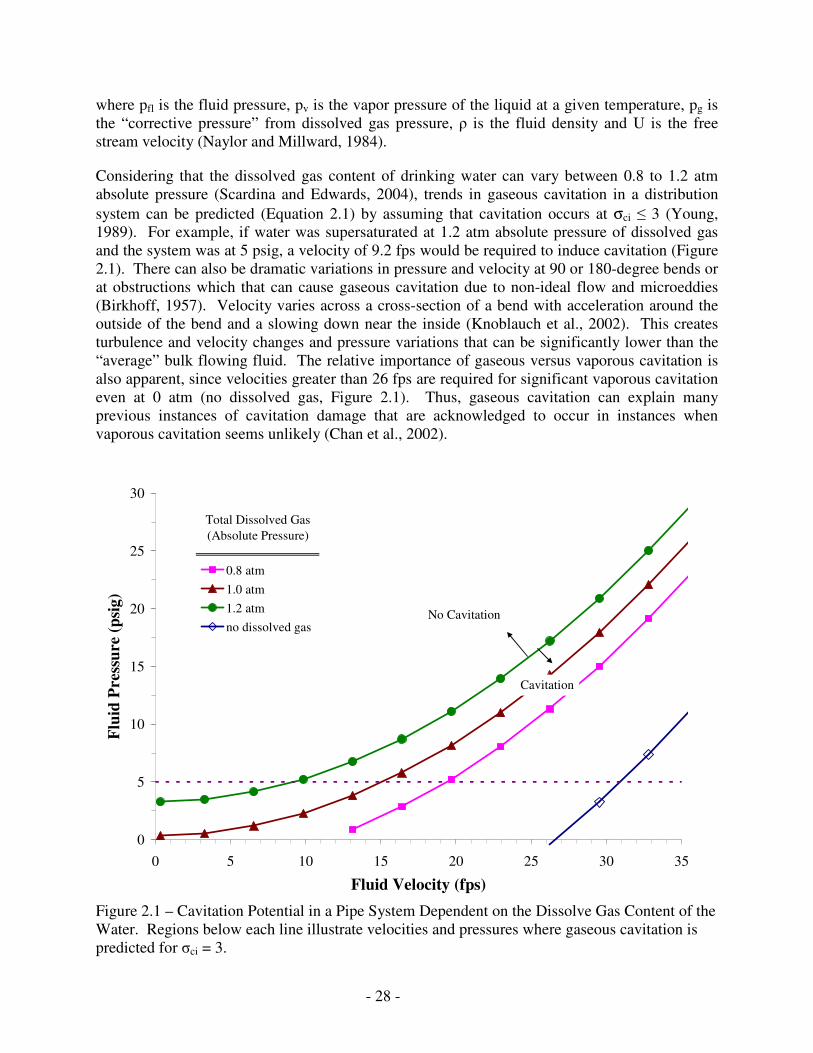
where pfl is the fluid pressure, pv is the vapor pressure of the liquid at a given temperature, pg is the “corrective pressure” from dissolved gas pressure, � is the fluid density and U is the free stream velocity (Naylor and Millward, 1984).

Considering that the dissolved gas content of drinking water can vary between 0.8 to 1.2 atm absolute pressure (Scardina and Edwards, 2004), trends in gaseous cavitation in a distribution system can be predicted (Equation 2.1) by assuming that cavitation occurs at σci � 3 (Young, 1989). For example, if water was supersaturated at 1.2 atm absolute pressure of dissolved gas and the system was at 5 psig, a velocity of 9.2 fps would be required to induce cavitation (Figure 2.1). There can also be dramatic variations in pressure and velocity at 90 or 180-degree bends or at obstructions which that can cause gaseous cavitation due to non-ideal flow and microeddies (Birkhoff, 1957). Velocity varies across a cross-section of a bend with acceleration around the outside of the bend and a slowing down near the inside (Knoblauch et al., 2002). This creates turbulence and velocity changes and pressure variations that can be significantly lower than the “average” bulk flowing fluid. The relative importance of gaseous versus vaporous cavitation is also apparent, since velocities greater than 26 fps are required for significant vaporous cavitation even at 0 atm (no dissolved gas, Figure 2.1). Thus, gaseous cavitation can explain many previous instances of cavitation damage that are acknowledged to occur in instances when vaporous cavitation seems unlikely (Chan et al., 2002).

0

5

10

15

20

25

30

0 5 10 15 20 25 30 35

Fluid Velocity (fps)

Flui

d Pr

essu

re (p

sig)

0.8 atm1.0 atm1.2 atmno dissolved gas

Total Dissolved Gas (Absolute Pressure)

No Cavitation

Cavitation

Figure 2.1 – Cavitation Potential in a Pipe System Dependent on the Dissolve Gas Content of the Water. Regions below each line illustrate velocities and pressures where gaseous cavitation is predicted for �ci = 3.

- 29 -

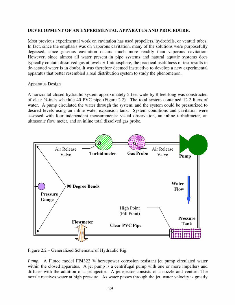
DEVELOPMENT OF AN EXPERIMENTAL APPARATUS AND PROCEDURE. Most previous experimental work on cavitation has used propellers, hydrofoils, or venturi tubes. In fact, since the emphasis was on vaporous cavitation, many of the solutions were purposefully degassed, since gaseous cavitation occurs much more readily than vaporous cavitation. However, since almost all water present in pipe systems and natural aquatic systems does typically contain dissolved gas at levels ≈ 1 atmosphere, the practical usefulness of test results in de-aerated water is in doubt. It was therefore deemed instructive to develop a new experimental apparatus that better resembled a real distribution system to study the phenomenon. Apparatus Design A horizontal closed hydraulic system approximately 5-feet wide by 8-feet long was constructed of clear ¾-inch schedule 40 PVC pipe (Figure 2.2). The total system contained 12.2 liters of water. A pump circulated the water through the system, and the system could be pressurized to desired levels using an inline water expansion tank. System conditions and cavitation were assessed with four independent measurements: visual observation, an inline turbidimeter, an ultrasonic flow meter, and an inline total dissolved gas probe.

Figure 2.2 – Generalized Schematic of Hydraulic Rig. Pump. A Flotec model FP4322 ¾ horsepower corrosion resistant jet pump circulated water within the closed apparatus. A jet pump is a centrifugal pump with one or more impellers and diffuser with the addition of a jet ejector. A jet ejector consists of a nozzle and venturi. The nozzle receives water at high pressure. As water passes through the jet, water velocity is greatly

Clear PVC Pipe Pressure

Tank Flowmeter

Turbidimeter Gas Probe Pump

90 Degree Bends

Pressure Gauge

Water Flow

Air Release Valve

Air Release Valve

High Point (Fill Point)

- 30 -

increased, but the pressure drops. The increased water speed, plus the lower pressure, causes suction around the nozzle. Water around the nozzle is drawn into the water stream and carried along with it. The nozzle and venturi combination (the jet ejector) changes the high-speed jet stream back to a high-pressure for delivery to the impeller eye. On this shallow well jet pump, the jet ejector is located in the pump housing in front of the impeller. The pump provides constant flow and was constructed of rugged fiberglass-reinforced thermoplastic that can operate at up to 100 psig. This pump was chosen based on the manufacturer’s opinion that minimal cavitation was expected at the impeller because of its design. Pumps delivering similar velocities are routinely installed in many newer homes in systems using hot water recirculation. Pressure Tank. An inline water expansion tank (Watts Series ILT-5) maintained a constant fluid pressure throughout the system and could sustain between 5 to 150 psig (± 1 psi). This tank consisted of an outer galvanized steel housing with an inner copper pipe and a butyl bladder that could be pressurized with air and depressurized via a common shrader valve. The use of this device allowed the static hydraulic pressure of the system to be set independent of the velocity. Laboratory experiments were conducted at constant pressures between 10 and 70 psig, as confirmed by a pressure gauge located directly in the pipe (Figure 2.2). Visual Observations. Since the rig was constructed mostly of clear pipe, visual observations could sometimes be used to identify when bubbles were present. The exact amount and diameter of bubbles in the system could not be determined from visual observations due to the high fluid velocity and since the bubbles usually migrated to the top of the pipe after the pump was stopped. However, some general trends were observed. For example, the number and size of bubbles increased at lower system pressures and could be made to completely disappear at higher pressures. Although the apparent bubble size increase is partly due to the lower pressures (i.e. Boyle’s Law), these relationships could not explain the magnitude of changes observed. For example, the ideal gas law predicted that a 1 mm diameter bubble at 70 psig would only grow to 1.5 mm diameter at 10 psig if the change were strictly due to a drop in pressure. In the tests, visual estimates indicated that bubble size increase by 3,000% versus the 50% predicted by the ideal gas law. This suggests that other factors control the size of bubbles that are present. In addition to the semi-quantitative visual observations regarding the quantity of bubbles, the sound of the pump was also noted to increase markedly as the pressure decreased throughout the course of each experiment, consistent with the onset of cavitation Ultrasonic Flowmeter. The Dynasonics Series 901 Enhanced Ultrasonic Doppler Flowmeter consisted of two transducers mounted on the outside of the pipe and can be used on pipes ranging in size from .25 inches to 120 inches in diameter. An ultrasonic sound wave emitted from the transmitting transducer through the pipe wall into the flowing water created a frequency shift via Doppler effect when the sound wave was reflected by suspended particles or bubbles in the liquid. The frequency shift is then translated to a velocity of flowing water (±2% of full scale). Accurate operation of this flowmeter was dependent on generation of an adequate reflected signal strength, and the manufacturer reports that at least 25 ppm of particles or bubbles are required. Given this dependency, the meter’s measurement of signal strength was investigated as a possible measure of total bubble concentration during flow, since all waters tested contained negligible turbidity. The device would not detect water velocity if bubbles were absent. There are eight levels of signal strength displayed on the meter, and practical experience demonstrates that if signal strength was below 6 the velocity measurements were not

- 31 -

reliable. But testing confirmed that the meter would not measure velocity in this system without added particles unless bubbles were present. Turbidimeter. The HACH Optiquant brand Suspended Solids and Turbidity (SST) Probe was placed inline directly in the pipe system and measured turbidity in conformity with ISO 7027 using a scattered light process. The probe had a measurement range of 0.010 to 1000 NTU and could detect particles or bubbles (Scardina and Edwards, 2002). The turbidimeter was installed in a white PVC 4-inch tee along the centerline of the water flow. The turbidity was calibrated as per manufacturer’s recommendations, with the exception that a background signal of 8 to 10 NTU had to be subtracted in particle free water due to reflection of light off the white pipe material used in the apparatus. Since the turbidimeter operates on a light scattering process, it cannot give an indication of the size of the bubbles in this system. While smaller bubbles tend to be registered by the instrument the same as particles, light scattering on large bubbles behaves very differently than on large particles. It was observed that the measured turbidity usually correlated well to visual trends. Gas Probe. The water’s total dissolved gas (TDG) was measured with a Common Sensing Inc. model TBO-L total dissolved gas probe (TDGP), which has been previously used successfully to quantify dissolved gases in solution (Scardina and Edwards, 2002). The probe can measure from 0 to 2 atmospheres (±2 mmHg) absolute pressure of total dissolved gas and is reported to be capable of accurate measurements at up to 150 psi. The probe also was equipped to measure dissolved oxygen up to 1 atmosphere (± 3 mmHg) absolute pressure, which was calibrated daily based upon the barometric pressure also measured by this instrument. The TDG and dissolved oxygen measurements are independent of one another. The probe also measures temperature up to 50º Celsius (± 0.1ºC ). Due to the size of the probe, it was installed in a clear 3 liter filter casing modified so that water moved past the probe and then back into the ¾-inch piping. Based on the lowest average flow, the solution residence time in the filter casing was 6 seconds, so the solution around the probe was assumed representative of that within the pipes. The TDG probe did not function reliably when the pump was in operation; according to the manufacturer, the internal membrane required 15 minutes for an accurate measurement. The TDGP was used for conditions at the beginning and end of the run to obtain measurements of TDG, oxygen and temperature. A stirbar at the bottom of the filter casing kept the solution in the casing well mixed during the measurement. Procedure The water was typically saturated with respect to the atmosphere by aeration for a minimum of 12 hours. No particles were added and other chemicals were dosed as necessary to create a target water quality. The entire rig was filled with the new water to be tested. During filling of the rig, all attempts were made to remove any “trapped” air, since this air could interfere with the experiments. After the initial fill, the system was pressurized to 70 psi, and the pump was run briefly to sweep out trapped air pockets which were collected in standpipes that could be opened to release trapped air. The system was then filled with additional water. This sequence was repeated three times, at which point much of the trapped air had been removed from the system and a consistent initial TDG content within +/- 5% of targeted values could be obtained, with the exception of a few outlier cases explicitly discussed in later text.

- 32 -

Some air still would remain trapped in the system, since water cannot completely wet solid surfaces due to its higher surface tension. Therefore, pre-existing gas pockets are left in small cracks and crevices. This trapped air can serve as nuclei for bubble formation in a mechanism known as heterogeneous nucleation (Harvey, 1975), similar to carbonated beverages. The initial temperature of the water could be adjusted to higher values by operating the pump for a period of time, which heated the water until the desired temperature was reached. Lower temperatures were maintained by allowing the entire apparatus to sit for a period of time. In this manner, a constant temperature could be maintained to within +/- 1 degrees C. Test Conditions. There were two types of experimental runs. The first group examined the effects of initial dissolved gas saturation and temperature. Experimental runs were performed for distilled water that was undersaturated, saturated, or supersaturated with respect to the atmosphere at temperatures of 30 and 45 degrees Celsius. The second group of tests examined various water qualities/chemistries at approximately constant temperature and initial degree of saturation. Four different pH’s were tested using either sodium hydroxide or hydrochloric acid to increase or decrease the pH, respectively. In all of these tests, sodium chloride was added to a level of 10-2 M, which maintained conductivity at 1.1 mS (+/- .3 mS), High pH runs were also conducted using lime (calcium hydroxide) without the NaCl to increase the conductivity from 0.03 mS. Other water quality changes included a higher conductivity, adding soluble natural organic matter (NOM) isolated from a lake and dosed to a final concentration of 0.5 or 2.8 mg C/L NOM, and two different common corrosion inhibitors (and surfactants) including sodium orthophosphate and hexametaphosphate were both dosed to 1 mg P/L. The carbon concentration and phosphorus were measured with a Sievers 800 Total Organic Carbon Analyzer and a JY Ultima ICP-ES (inductively coupled plasma with emission spectroscopy), respectively. In a typical experiment, water was made up at the desired chemistry, and the system was initiated to sweep out trapped gas and achieve the targeted temperature and initial level of gas supersaturation. An experiment began by measuring initial total dissolved gas and dissolved oxygen with the TDGP and stagnant water turbidity with the inline turbidimeter (to establish background NTU). The pump was then operated for 1 minute, during which time 10 separate measurements were made for turbidity, fluid velocity, and the signal strength of the flowmeter. Velocity was measured after 30 seconds. Experience showed that operating the pump for longer than 1 minute did not change the experimental results, aside from those expected due to increasing temperature. After 1 minute, the pump is stopped and total dissolved gas, oxygen, and turbidity readings were taken after 15 minutes as required for the TDG measurements, thus completing a test. The experiment was then re-started at a lower system pressure achieved by releasing a valve on the pressure tank, and the pump was run to return the system to the experimental protocol temperature. An experiment was ended after final measurements for the total system pressure of 10 psig. The experimental apparatus was then emptied completely and rinsed thoroughly. Though not done with every run, in a few experiments, the water was not emptied immediately after the experiment but instead the rig was repressurized and the water was recirculated via the pump.

- 33 -

Each time it took less than 2 minutes of the pump running for the turbidity readings to stabilize at non-detectable levels. Determination of Bubble Volume. The total dissolved gas probe gave a direct, in-system reading of any loss of dissolved gas from the water during the experiment. Any loss in TDG from the water during a run was due to gases leaving solution to form bubbles. Likewise, an increase in TDG would be attributed to dissolution of gas into the water from the pre-existing trapped air pockets. Henry’s gas law could be used to convert the measured dissolved gas partial pressures to concentrations and bubble volume (V) was estimated using the Ideal Gas Law (Equations 2.2 and 2.3) at the system temperature (T) and pressure (P):

[ ] gas*H pK Gas = (Equation 2.2)

PnRT

V = (Equation 2.3)

where pgas is the measured partial pressure of a gas in absolute pressure, KH is Henry’s Gas Law constant adjusted for temperature, n is the sum of the molar concentrations of each gas in solution (�[Gas]), and R is a constant. The TDG measurement can be assumed to be the sum of the oxygen and nitrogen partial pressures, in which case the partial pressure of nitrogen is the difference between the absolute pressures of the measured TDG and that predicted based on Henry’s law (Equation 2.2) and the measured dissolved oxygen (Scardina and Edwards, 2004, II). Less than 0.035% of the total dissolved gas pressure in this system using distilled water is expected to be due to CO2. Any reduction in moles of dissolved gas in the water during a run is assumed to equal the moles of gas (n) in bubbles (Equation 2.3) RESULTS. The data from a typical experiment is introduced first, followed by results from each group of experiments: saturation/temperature and varying water qualities. The important effects of gaseous cavitation on pump operational efficiency are also introduced. A Typical Experimental Run

After filling the apparatus and stabilizing the initial conditions, the system was pressurized and operated at 70 psig, and then stepped down to 10 psig in 10 psi increments. No bubbles were definitively detected by any of the four methods at 70 or 60 psig. Bubbles first became visible at a system pressure of 50 psig at approximately 1 mm in diameter (Figure 2.3). The bubble diameters increased as the system pressure decreased and were as large as 30 mm at 10 psig. Calculations of bubble volume formed suggested that 0.2% of the total flow was gas bubbles. Due to the speed of the water flow, visual observations could not determine the exact location at which bubbles were originating. Immediately after stopping the pump, approximately 25% more bubbles appeared to be present after a bend than before it. As water was flowing through the pipes, the bubbles did not travel in the middle of the flow stream after a bend, but rather in a sinusoidal pattern where the bubbles impacted opposing sides of the pipe. The sinusoidal bubble flow pattern was not a function of bubble size or system pressure and remained stable over time

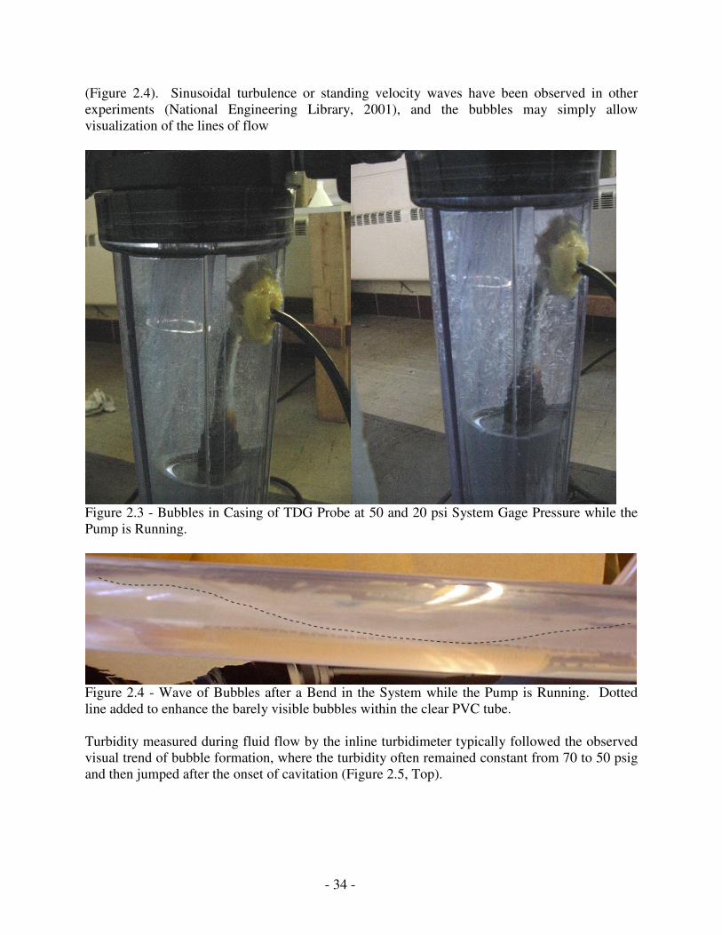
- 34 -

(Figure 2.4). Sinusoidal turbulence or standing velocity waves have been observed in other experiments (National Engineering Library, 2001), and the bubbles may simply allow visualization of the lines of flow

Figure 2.3 - Bubbles in Casing of TDG Probe at 50 and 20 psi System Gage Pressure while the Pump is Running.

Figure 2.4 - Wave of Bubbles after a Bend in the System while the Pump is Running. Dotted line added to enhance the barely visible bubbles within the clear PVC tube. Turbidity measured during fluid flow by the inline turbidimeter typically followed the observed visual trend of bubble formation, where the turbidity often remained constant from 70 to 50 psig and then jumped after the onset of cavitation (Figure 2.5, Top).

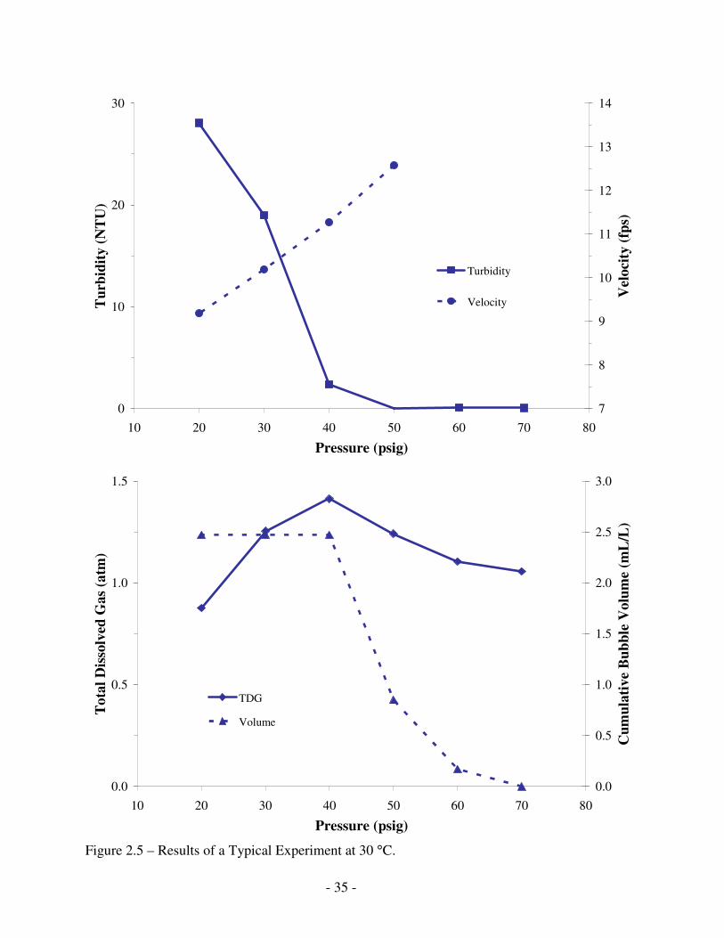
- 35 -

0

10

20

30

10 20 30 40 50 60 70 80

Pressure (psig)

Tur

bidi

ty (N

TU

)

7

8

9

10

11

12

13

14

Vel

ocity

(fps

)

Turbidity

Velocity

0.0

0.5

1.0

1.5

10 20 30 40 50 60 70 80

Pressure (psig)

Tot

al D

isso

lved

Gas

(atm

)

0.0

0.5

1.0

1.5

2.0

2.5

3.0

Cum

ulat

ive

Bub

ble

Vol

ume

(mL

/L)

TDG

Volume

Figure 2.5 – Results of a Typical Experiment at 30 °C.

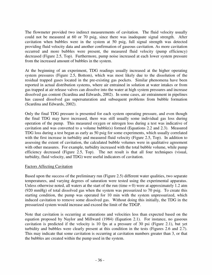
- 36 -

The flowmeter provided two indirect measurements of cavitation. The fluid velocity usually could not be measured at 60 or 70 psig, since there was inadequate signal strength. After cavitation when bubbles were in the system at 50 psig, full signal strength was detected providing fluid velocity data and another confirmation of gaseous cavitation. As more cavitation occurred and more bubbles were present, the measured fluid velocity (pump efficiency) decreased (Figure 2.5, Top). Furthermore, pump noise increased at each lower system pressure from the increased amount of bubbles in the system. At the beginning of an experiment, TDG readings usually increased at the higher operating system pressures (Figure 2.5, Bottom), which was most likely due to the dissolution of the residual trapped gases located in the pre-existing gas pockets. Similar phenomena have been reported in actual distribution systems, where air entrained in solution at water intakes or from gas trapped at air release valves can dissolve into the water at high system pressures and increase dissolved gas content (Scardina and Edwards, 2002). In some cases, air entrainment in pipelines has caused dissolved gas supersaturation and subsequent problems from bubble formation (Scardina and Edwards, 2002). Only the final TDG pressure is presented for each system operating pressure, and even though the final TDG may have increased, there was still usually some individual gas loss during operation of the pump. This measured oxygen or nitrogen loss during a test was indicative of cavitation and was converted to a volume bubble(s) formed (Equations 2.2 and 2.3). Measured TDG loss during a test began as early as 50 psig for some experiments, which usually correlated with the first increase in turbidity and measured fluid velocity (Figure 2.5, Top). In addition to assessing the extent of cavitation, the calculated bubble volumes were in qualitative agreement with other measures. For example, turbidity increased with the total bubble volume, while pump efficiency decreased (Figure 2.5, Top). The net result is that all four techniques (visual, turbidity, fluid velocity, and TDG) were useful indicators of cavitation. Factors Affecting Cavitation Based upon the success of the preliminary run (Figure 2.5) different water qualities, two separate temperatures, and varying degrees of saturation were tested using the experimental apparatus. Unless otherwise noted, all waters at the start of the run (time = 0) were at approximately 1.2 atm (920 mmHg) of total dissolved gas when the system was pressurized to 70 psig. To create this starting condition, the pump was operated for 10 min with the system unpressurized, which induced cavitation to remove some dissolved gas. Without doing this initially, the TDG in the pressurized system would increase and exceed the limit of the TDGP. Note that cavitation is occurring at saturations and velocities less than expected based on the equation proposed by Naylor and Millward (1984) (Equation 2.1). For instance, no gaseous cavitation is predicted if the velocity is 10 fps at a pressure of 30 psi (Figure 2.1), but yet turbidity and bubbles were clearly present at this condition in the tests (Figures 2.6 and 2.7). This may indicate that some cavitation is occurring at cavitation numbers greater than 3, or that the bubbles are created within the pump used in the system.

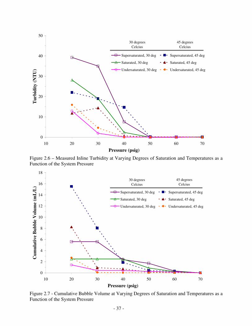
- 37 -

0

10

20

30

40

50

10 20 30 40 50 60 70

Pressure (psig)

Tur

bidi

ty (N

TU

)

Supersaturated, 30 deg Supersaturated, 45 deg

Saturated, 30 deg Saturated, 45 deg

Undersaturated, 30 deg Undersaturated, 45 deg

30 degrees Celcius

45 degrees Celcius

Figure 2.6 – Measured Inline Turbidity at Varying Degrees of Saturation and Temperatures as a Function of the System Pressure

0

2

4

6

8

10

12

14

16

18

10 20 30 40 50 60 70

Pressure (psig)

Cum

ulat

ive

Bub

ble

Vol

ume

(mL

/L)

Supersaturated, 30 deg Supersaturated, 45 deg

Saturated, 30 deg Saturated, 45 deg

Undersaturated, 30 deg Undersaturated, 45 deg

30 degrees Celcius

45 degrees Celcius

Figure 2.7 - Cumulative Bubble Volume at Varying Degrees of Saturation and Temperatures as a Function of the System Pressure

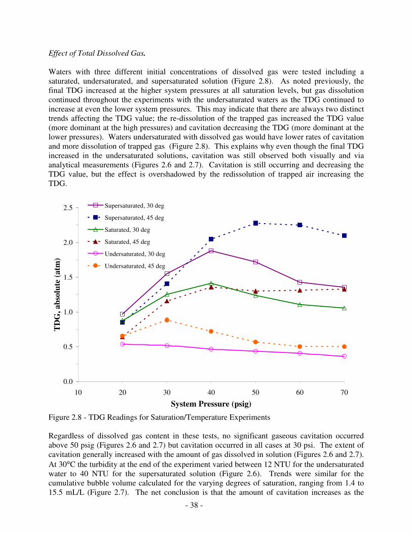
- 38 -

Effect of Total Dissolved Gas. Waters with three different initial concentrations of dissolved gas were tested including a saturated, undersaturated, and supersaturated solution (Figure 2.8). As noted previously, the final TDG increased at the higher system pressures at all saturation levels, but gas dissolution continued throughout the experiments with the undersaturated waters as the TDG continued to increase at even the lower system pressures. This may indicate that there are always two distinct trends affecting the TDG value; the re-dissolution of the trapped gas increased the TDG value (more dominant at the high pressures) and cavitation decreasing the TDG (more dominant at the lower pressures). Waters undersaturated with dissolved gas would have lower rates of cavitation and more dissolution of trapped gas (Figure 2.8). This explains why even though the final TDG increased in the undersaturated solutions, cavitation was still observed both visually and via analytical measurements (Figures 2.6 and 2.7). Cavitation is still occurring and decreasing the TDG value, but the effect is overshadowed by the redissolution of trapped air increasing the TDG.

0.0

0.5

1.0

1.5

2.0

2.5

10 20 30 40 50 60 70

System Pressure (psig)

TD

G, a

bsol

ute

(atm

)

Supersaturated, 30 deg

Supersaturated, 45 deg

Saturated, 30 deg

Saturated, 45 deg

Undersaturated, 30 deg

Undersaturated, 45 deg

Figure 2.8 - TDG Readings for Saturation/Temperature Experiments Regardless of dissolved gas content in these tests, no significant gaseous cavitation occurred above 50 psig (Figures 2.6 and 2.7) but cavitation occurred in all cases at 30 psi. The extent of cavitation generally increased with the amount of gas dissolved in solution (Figures 2.6 and 2.7). At 30°C the turbidity at the end of the experiment varied between 12 NTU for the undersaturated water to 40 NTU for the supersaturated solution (Figure 2.6). Trends were similar for the cumulative bubble volume calculated for the varying degrees of saturation, ranging from 1.4 to 15.5 mL/L (Figure 2.7). The net conclusion is that the amount of cavitation increases as the

- 39 -

amount of dissolved gas increases, but the threshold pressure at which cavitation begins to occur in these experiments was relatively insensitive to dissolved gas. Practically, this demonstrates that it may be easiest to control gaseous cavitation by increasing pressure, since it is difficult to decrease dissolved gas content. Effects of Temperature. The effects 30° and 45° C temperatures were examined within the first group of experiments at various saturation levels. The system temperature was controlled by operation of the pump which tended to heat the water over time. The turbidity at the cooler temperature was generally higher than at the higher temperature (Figure 2.6). These results are consistent with previous predictions in a jar test coagulation study (Scardina and Edwards, 2004). When the Scardina and Edwards bubble equilibrium model (2001) is used to predict bubble formation, the colder solution is predicted to form more gas bubbles for similar initial conditions. This tendency appears to overcome slower mass transfer kinetics at lower temperatures. Yet, the cumulative bubble volumes for each level of saturation were greater in the higher temperature waters (Figure 2.7). Although part of this may be due to an overall higher absolute TDG value at corresponding saturation values (Figure 2.8), it is unlikely that is enough to completely account for the effect. Surface tension is inversely related to temperature so at the higher temperatures, the water has a lower surface tension that perhaps allows for more rapid bubble growth. There were two distinct trends for gaseous cavitation with respect to temperature. At the higher temperatures, there was a marked increase in calculated bubble volume and greater difference in total dissolved gas (Figures 2.8 and 2.5). This would indicate more cavitation as measured by volume of gas at the high temperatures versus the lower temperatures; however, at the same time the higher temperature water had markedly lower turbidity readings (Figure 2.6). This may indicate that while the colder temperature formed more bubbles as measured by the turbidimeter, they were smaller in size relative to the higher temperature bubbles. The turbidimeter also detects bubbles sizes differently; although smaller bubbles react very similar to particles, larger bubbles reflect light very differently than solid particles. Water Quality. A variety of water qualities were examined at a constant system temperature and initial TDG (Table 2.1). It is unclear why the pH 9.9 with lime started with a higher initial TDG and the 2.78 mg/L-C NOM started lower. It is presumed that even though the same procedure was followed, the initial 10 minute degassing may have been more less effective at higher pH than with the NOM. Surprisingly, pH had a largest effect on cavitation (Figures 2.9 and 2.10). The pH of the control was 5.0 and the other solutions with a similar pH (4.0 and 5.0) were not radically different from the control. As the pH increased more cavitation occurred. Compared to the control at 30 psig system pressure, the turbidity increased 30% and 295% at pH 8.5 and 9.9, respectively. The exact reason for this effect is not certain. When the conditions were repeated with lime (CaOH), the turbidity increase was less dramatic (49%) than for caustic at pH 9.9 (Figure 2.9). Solution conductivity may have some influence on the bubble formation in the

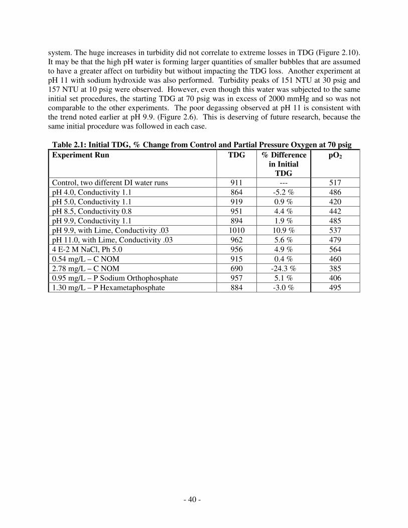
- 40 -

system. The huge increases in turbidity did not correlate to extreme losses in TDG (Figure 2.10). It may be that the high pH water is forming larger quantities of smaller bubbles that are assumed to have a greater affect on turbidity but without impacting the TDG loss. Another experiment at pH 11 with sodium hydroxide was also performed. Turbidity peaks of 151 NTU at 30 psig and 157 NTU at 10 psig were observed. However, even though this water was subjected to the same initial set procedures, the starting TDG at 70 psig was in excess of 2000 mmHg and so was not comparable to the other experiments. The poor degassing observed at pH 11 is consistent with the trend noted earlier at pH 9.9. (Figure 2.6). This is deserving of future research, because the same initial procedure was followed in each case.

Table 2.1: Initial TDG, % Change from Control and Partial Pressure Oxygen at 70 psig Experiment Run TDG % Difference

in Initial TDG

pO2

Control, two different DI water runs 911 --- 517 pH 4.0, Conductivity 1.1 864 -5.2 % 486 pH 5.0, Conductivity 1.1 919 0.9 % 420 pH 8.5, Conductivity 0.8 951 4.4 % 442 pH 9.9, Conductivity 1.1 894 1.9 % 485 pH 9.9, with Lime, Conductivity .03 1010 10.9 % 537 pH 11.0, with Lime, Conductivity .03 962 5.6 % 479 4 E-2 M NaCl, Ph 5.0 956 4.9 % 564 0.54 mg/L – C NOM 915 0.4 % 460 2.78 mg/L – C NOM 690 -24.3 % 385 0.95 mg/L – P Sodium Orthophosphate 957 5.1 % 406 1.30 mg/L – P Hexametaphosphate 884 -3.0 % 495

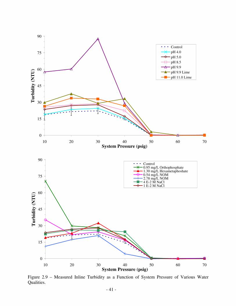
- 41 -

0

15

30

45

60

75

90

10 20 30 40 50 60 70System Pressure (psig)

Tur

bidi

ty (N

TU

)

ControlpH 4.0pH 5.0pH 8.5pH 9.9pH 9.9 LimepH 11.0 Lime

0

15

30

45

60

75

90

10 20 30 40 50 60 70System Pressure (psig)

Tur

bidi

ty (N

TU

)

Control0.95 mg/L Orthophosphate1.30 mg/L Hexametaphoshate0.54 mg/L NOM2.78 mg/L NOM4 E-2 M NaCl1 E-2 M NaCl

Figure 2.9 – Measured Inline Turbidity as a Function of System Pressure of Various Water Qualities.

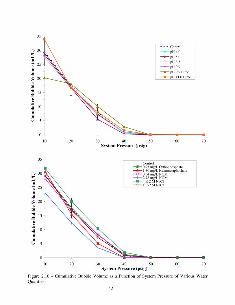
- 42 -

0

5

10

15

20

25

30

35

10 20 30 40 50 60 70System Pressure (psig)

Cum

ulat

ive

Bub

ble

Vol

ume

(mL

/L) Control

pH 4.0pH 5.0pH 8.5pH 9.9pH 9.9 LimepH 11.0 Lime

0

5

10

15

20

25

30

35

10 20 30 40 50 60 70System Pressure (psig)

Cum

ulat

ive

Bub

ble

Vol

ume

(mL

/L)

Control0.95 mg/L Orthophosphate1.30 mg/L Hexametaphoshate0.54 mg/L NOM2.78 mg/L NOM4 E-2 M NaCl1 E-2 M NaCl

Figure 2.10 – Cumulative Bubble Volume as a Function of System Pressure of Various Water Qualities.

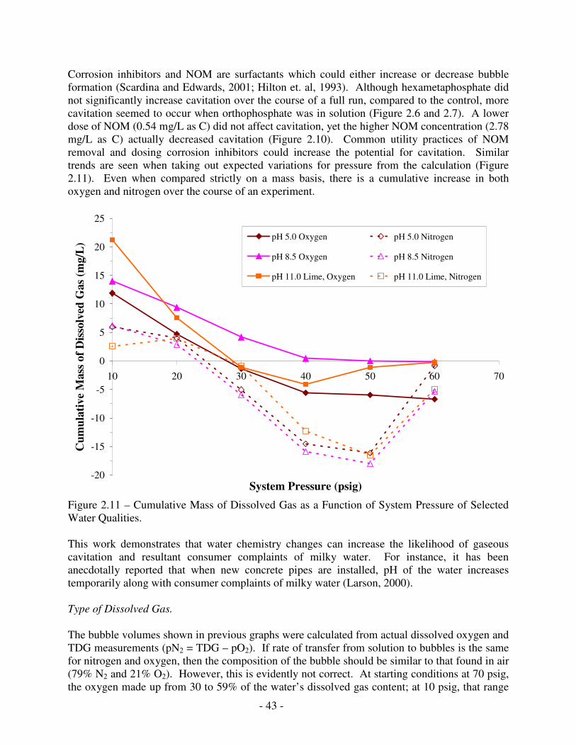
- 43 -

Corrosion inhibitors and NOM are surfactants which could either increase or decrease bubble formation (Scardina and Edwards, 2001; Hilton et. al, 1993). Although hexametaphosphate did not significantly increase cavitation over the course of a full run, compared to the control, more cavitation seemed to occur when orthophosphate was in solution (Figure 2.6 and 2.7). A lower dose of NOM (0.54 mg/L as C) did not affect cavitation, yet the higher NOM concentration (2.78 mg/L as C) actually decreased cavitation (Figure 2.10). Common utility practices of NOM removal and dosing corrosion inhibitors could increase the potential for cavitation. Similar trends are seen when taking out expected variations for pressure from the calculation (Figure 2.11). Even when compared strictly on a mass basis, there is a cumulative increase in both oxygen and nitrogen over the course of an experiment.

-20

-15

-10

-5

0

5

10

15

20

25

10 20 30 40 50 60 70

System Pressure (psig)

Cum

ulat

ive

Mas

s of D

isso

lved

Gas

(mg/

L) pH 5.0 Oxygen pH 5.0 Nitrogen

pH 8.5 Oxygen pH 8.5 Nitrogen

pH 11.0 Lime, Oxygen pH 11.0 Lime, Nitrogen

Figure 2.11 – Cumulative Mass of Dissolved Gas as a Function of System Pressure of Selected Water Qualities. This work demonstrates that water chemistry changes can increase the likelihood of gaseous cavitation and resultant consumer complaints of milky water. For instance, it has been anecdotally reported that when new concrete pipes are installed, pH of the water increases temporarily along with consumer complaints of milky water (Larson, 2000). Type of Dissolved Gas. The bubble volumes shown in previous graphs were calculated from actual dissolved oxygen and TDG measurements (pN2 = TDG – pO2). If rate of transfer from solution to bubbles is the same for nitrogen and oxygen, then the composition of the bubble should be similar to that found in air (79% N2 and 21% O2). However, this is evidently not correct. At starting conditions at 70 psig, the oxygen made up from 30 to 59% of the water’s dissolved gas content; at 10 psig, that range

- 44 -

was 16 to 35%. In other words, oxygen was disproportionately transferred to the bubbles. This is somewhat surprising, given that the diffusion rate constant for nitrogen is actually greater than that for oxygen. The effects of dissolved gas type deserve additional study.

Table 2.2: Percent Oxygen of TDG at Various Pressures Experiment Run 70 psig 40 psig 10 psig Control, two different DI water runs 57% 30% 28% pH 4.0, Conductivity 1.1 56% 28% 29% pH 5.0, Conductivity 1.1 46% 30% 33% pH 8.5, Conductivity 0.8 47% 26% 35% pH 9.9, Conductivity 1.1 54% 29% 30% pH 9.9, with Lime, Conductivity .03 53% 28% 27% pH 11.0, with Lime, Conductivity .03 50% 36% 16% 4 E-2 M NaCl, Ph 5.0 59% 31% 28% 0.54 mg/L – C NOM 50% 28% 29% 2.78 mg/L – C NOM 56% 31% 34% 0.95 mg/L – P Sodium Orthophosphate 42% 29% 30% 1.30 mg/L – P Hexametaphosphate 56% 31% 30% Note that 70 psig is a before pump run measurement, 40 and 10 psig measurements are after pump is run

Bubbles and Pump Efficiency A manufacturer’s pump curve indicates changes in discharge velocity as a function of pressure change across the pump (Figure 2.12). The pump can only operate along this pump curve. The relationship between bubbles and pump efficiency, though, is never explicitly considered in practice. In the absence of bubbles, pump operating efficiency should not be a strong function of total system pressure. This work demonstrates that when bubbles formed, pump operating efficiency and discharge velocity were a strong function of total pressure. Thus, the efficiency of the pump, as measured by the fluid velocity, was influenced by cavitation. Compared to a solution at 30° C, an increase in total dissolved gas levels decreased the efficiency of the pump, as did an increase in water temperature (Figure 2.13). Although there was always more bubble volume produced with higher degrees of saturation (Figure 2.7), supersaturated or undersaturated water both decreased the pump efficiency compared to saturated (Figure 2.13). It may be that a certain degree of dissolved gases are required for optimum pump operation; deviations above and below that degree of saturation decrease pump efficiency. Another parameter, such as actual bubble size or viscosity, could be influencing the results. Compared to water quality changes, changes in velocity were not as dramatic as those for various saturation levels, however they were evident even at high pressures. Theoretically an increased temperature would decrease the viscosity of the water and should result in an increase in pump efficiency, however the opposite was observed (Figure 2.13). This may indicate that bubble effects dominate over viscosity effects in pumping.

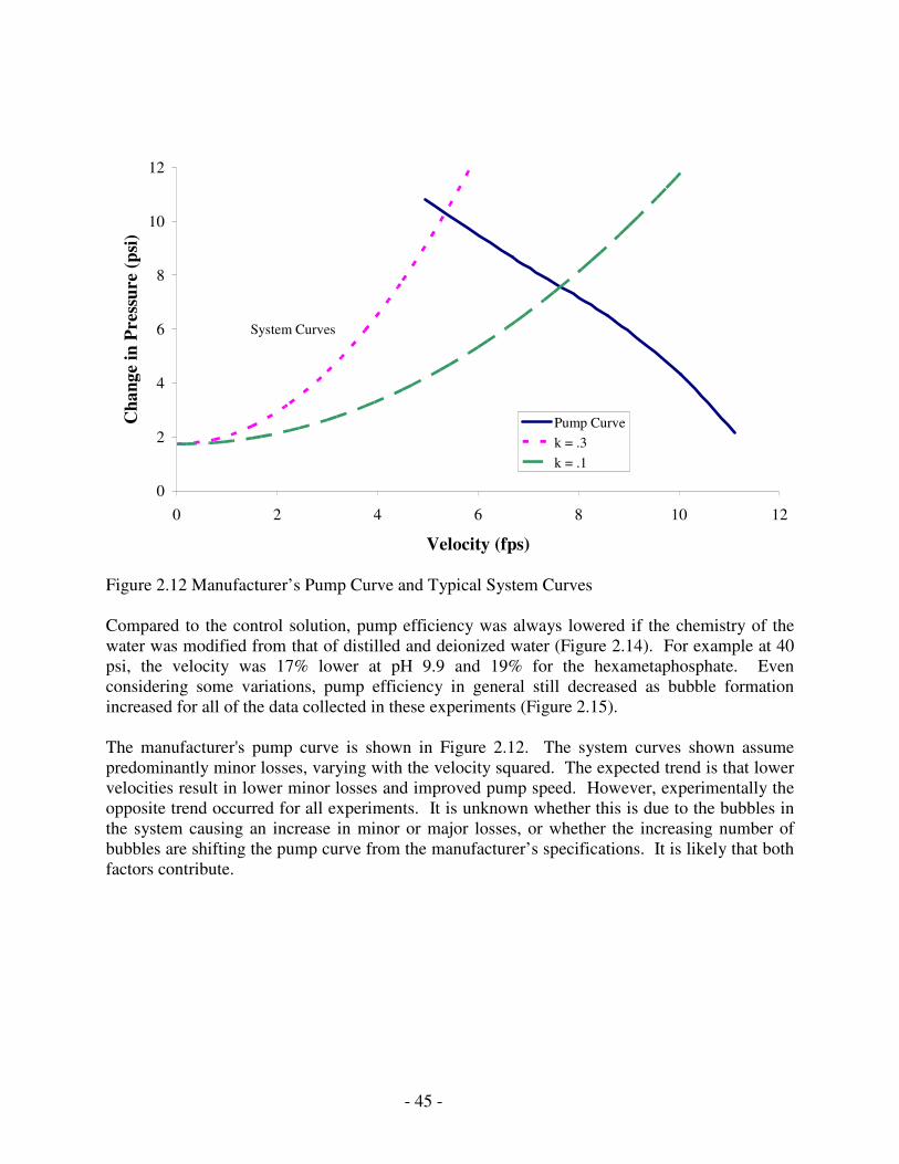
- 45 -

0

2

4

6

8

10

12

0 2 4 6 8 10 12

Velocity (fps)

Cha

nge

in P

ress

ure

(psi

)

Pump Curvek = .3k = .1

System Curves

Figure 2.12 Manufacturer’s Pump Curve and Typical System Curves Compared to the control solution, pump efficiency was always lowered if the chemistry of the water was modified from that of distilled and deionized water (Figure 2.14). For example at 40 psi, the velocity was 17% lower at pH 9.9 and 19% for the hexametaphosphate. Even considering some variations, pump efficiency in general still decreased as bubble formation increased for all of the data collected in these experiments (Figure 2.15). The manufacturer's pump curve is shown in Figure 2.12. The system curves shown assume predominantly minor losses, varying with the velocity squared. The expected trend is that lower velocities result in lower minor losses and improved pump speed. However, experimentally the opposite trend occurred for all experiments. It is unknown whether this is due to the bubbles in the system causing an increase in minor or major losses, or whether the increasing number of bubbles are shifting the pump curve from the manufacturer’s specifications. It is likely that both factors contribute.

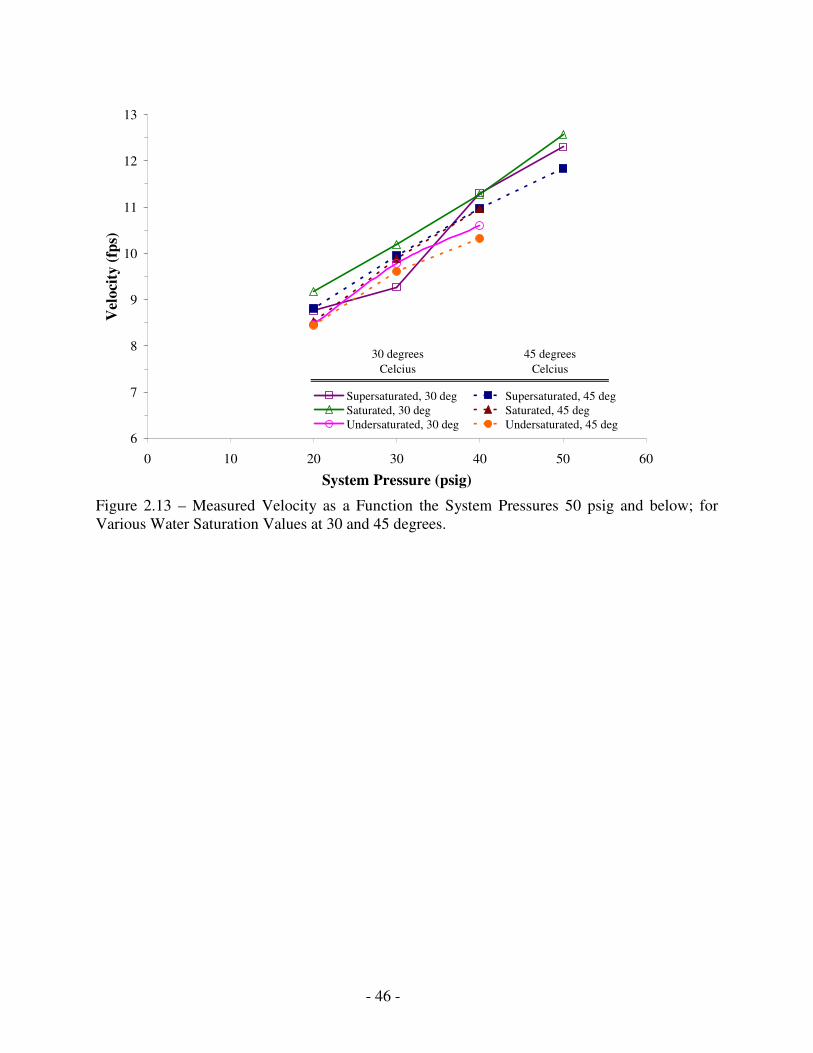
- 46 -

6

7

8

9

10

11

12

13

0 10 20 30 40 50 60

System Pressure (psig)

Vel

ocity

(fps

)

Supersaturated, 30 deg Supersaturated, 45 degSaturated, 30 deg Saturated, 45 degUndersaturated, 30 deg Undersaturated, 45 deg

30 degrees Celcius

45 degrees Celcius

Figure 2.13 – Measured Velocity as a Function the System Pressures 50 psig and below; for Various Water Saturation Values at 30 and 45 degrees.

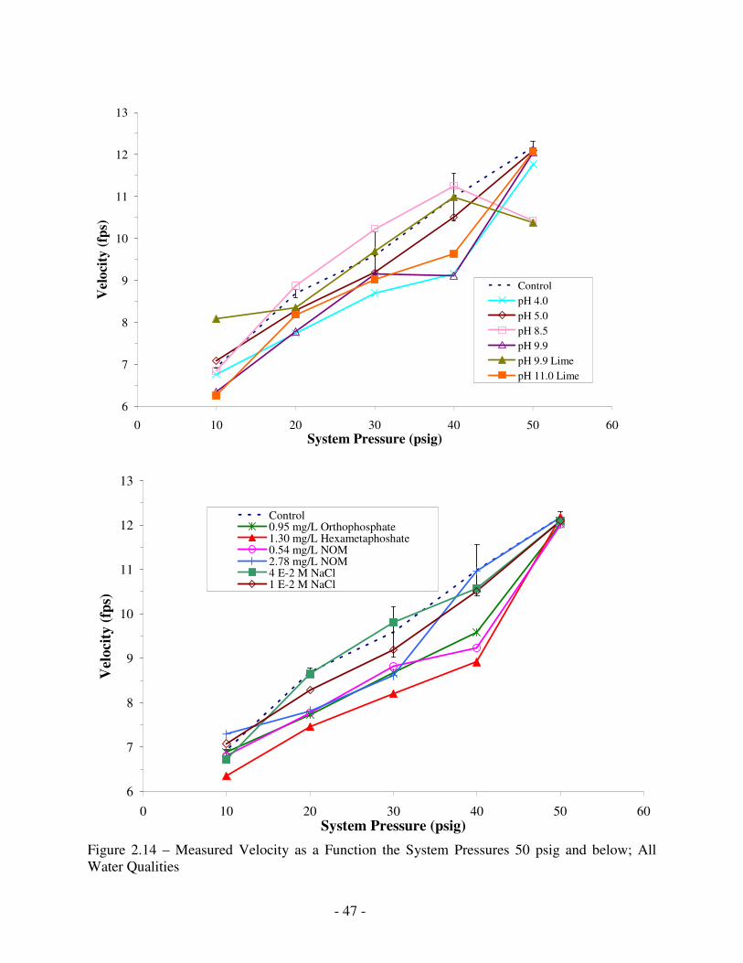
- 47 -

6

7

8

9

10

11

12

13

0 10 20 30 40 50 60System Pressure (psig)

Vel

ocity

(fps

)

ControlpH 4.0pH 5.0pH 8.5pH 9.9pH 9.9 LimepH 11.0 Lime

6

7

8

9

10

11

12

13

0 10 20 30 40 50 60System Pressure (psig)

Vel

ocity

(fps

)

Control0.95 mg/L Orthophosphate1.30 mg/L Hexametaphoshate0.54 mg/L NOM2.78 mg/L NOM4 E-2 M NaCl1 E-2 M NaCl

Figure 2.14 – Measured Velocity as a Function the System Pressures 50 psig and below; All Water Qualities

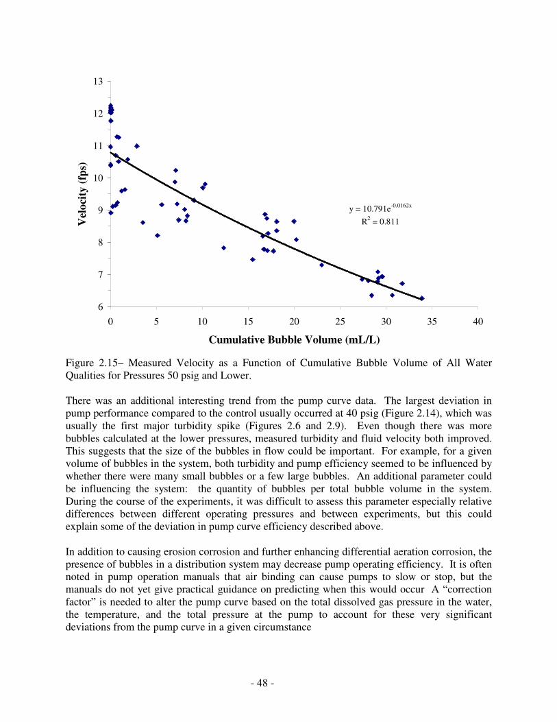
- 48 -

y = 10.791e-0.0162x

R2 = 0.811

6

7

8

9

10

11

12

13

0 5 10 15 20 25 30 35 40

Cumulative Bubble Volume (mL/L)

Vel

ocity

(fps

)

Figure 2.15– Measured Velocity as a Function of Cumulative Bubble Volume of All Water Qualities for Pressures 50 psig and Lower. There was an additional interesting trend from the pump curve data. The largest deviation in pump performance compared to the control usually occurred at 40 psig (Figure 2.14), which was usually the first major turbidity spike (Figures 2.6 and 2.9). Even though there was more bubbles calculated at the lower pressures, measured turbidity and fluid velocity both improved. This suggests that the size of the bubbles in flow could be important. For example, for a given volume of bubbles in the system, both turbidity and pump efficiency seemed to be influenced by whether there were many small bubbles or a few large bubbles. An additional parameter could be influencing the system: the quantity of bubbles per total bubble volume in the system. During the course of the experiments, it was difficult to assess this parameter especially relative differences between different operating pressures and between experiments, but this could explain some of the deviation in pump curve efficiency described above. In addition to causing erosion corrosion and further enhancing differential aeration corrosion, the presence of bubbles in a distribution system may decrease pump operating efficiency. It is often noted in pump operation manuals that air binding can cause pumps to slow or stop, but the manuals do not yet give practical guidance on predicting when this would occur A “correction factor” is needed to alter the pump curve based on the total dissolved gas pressure in the water, the temperature, and the total pressure at the pump to account for these very significant deviations from the pump curve in a given circumstance

- 49 -

Discussion In the experiments conducted with the pipe apparatus, cavitation occurred at saturations and velocities less than expected based on the equation proposed by Naylor and Millward (1984) (Equation 2.1). For instance, no gaseous cavitation is predicted if the velocity is 9 fps at a pressure of 20 psi (Figure 2.1), but yet turbidity and bubbles were clearly present at this testing condition (Figures 2.6 and 2.7). Non-ideal flow conditions occur at bends and other obstructions or the pump most likely created the conditions that allowed cavitation. The implication is that cavitation can occur in many systems in which it was not predicted to occur. The inline turbidimeter was a successful method of identifying cavitation. In fact, this probe was specifically designed for use in pipe systems, and a special adaptor can be purchased to make retrofitting into pipes easier. An advantage of this approach is the simplicity of data collection and interpretation since turbidity is a standard water quality parameter. A grab sample could be collected, degassed, and then measured with a bench top turbidimeter after it passed through the device to determine the turbidity due to particles. Any increase in turbidity during fluid flow would most likely be due to cavitation, although it is impossible to distinguish between bubbles and suspended particulates The turbidimeter provided inconsistent results at low system pressures. As mentioned previously, the turbidimeter had a counter-intuitive trend at low pressures. Even though cumulative bubble volume increased, turbidity was often decreased between 30 and 20 psi (Figures 2.9 and 2.10) even though visually larger bubble sizes were observed. This is likely due to the fact that the turbidimeter detects light scattering, and there is not a strong correlation between turbidity and total bubble volume (Figure 2.16).

- 50 -

R2 = 0.6345

R2 = 0.4067

0

10

20

30

40

50

60

70

80

90

100

0 5 10 15 20 25 30 35

Cumulative Bubble Volume (mL/L)

Tur

bidi

ty (N

TU

) 0.95 mg/L OrthophosphatepH 9.9All Other Water Qualities

Note: Trendlines based only on data series 'All Other Water Qualities'

Figure 2.16 – Measured Inline Turbidity as a Function of Calculated Bubble Volume of All Water Qualities. The curved trendline indicates while there is an overall increasing correlation between turbidity and bubble volume, the decreasing turbidity at lower pressures does affect the correlation. R2 values for linear trendlines for each individual water quality range from 0.22 to 0.87. Even though the total dissolved gas probe (TDGP) measurements were time consuming, it was a powerful tool for assessing bubble formation. Preliminary data suggested that more oxygen was present in bubbles than would be predicted based on Henry’s law and equilibrium consideration. It is possible that this results from a dynamic system in which bubbles are continually being destroyed and created, versus equilibrium. More data is necessary (Table 2.2). TDG measurements should become routine prior to designing a new system. Source waters naturally susceptible to dissolved gas supersaturation could be identified, so that systems could be designed and operated to limit cavitation or bubble formation. More air release valves are likely to be required in situations which are conducive to greater cavitation. A full analysis would also incorporate pH and alkalinity measurements to quantify dissolved carbon dioxide. These experiments were managed such that carbon dioxide was negligible, but carbon dioxide partial pressures can be high in drinking water (Scardina et al., 2005a,b). The ultrasonic flowmeter also proved useful in detecting cavitation. The instrument proved to be consistent with the other methods of identifying cavitation. For instance, a fluid velocity could not be measured at the higher operating pressures when bubbles were not present and cavitation was not occurring. The first indication of full signal strength on the flowmeter always coincided

- 51 -

with the first detected increase in turbidity (Figure 2.3). It is therefore anticipated that this flowmeter could be used in real systems to detect cavitation, as long as suspended particulates are low. This method is advantageous because is nondestructive to the pipe and can be installed anywhere on the pipe. If full signal strength is detected in a distribution system, then the flow rate can be gradually reduced to determine if cavitation or real particles are being detected by the instrument. If the signal disappears at lower flow rates, then cavitation is most likely occurring at the higher velocity. Furthermore, grab samples could be collected to confirm the presence of real particles in the solution. Attempts were made to utilize the weaker signals strengths (0 – 8 scale on instrument) as another detection tool for cavitation (Table 2.3). The fluid velocities at the lower signal strengths were indeed unreliable data, but a higher average signal strength at high pressures loosely correlated to an increased turbidity and cumulative bubble volume at lower pressures (Figure 2.17). This could have serious implications; even high pressures may be subject to a small amount of gaseous cavitation. Even single bubbles can have an impact on corrosion rates and bacterial growth in a pipe (Novak and Edwards, 2005).

Table 2.3: Average Signal Strengths on the Doppler Flowmeter at High Pressures Experiment Run 70 psig 60 psig 30 degree, Supersaturated 1.5 2.5 30 degree, Saturated 5 5 30 degree, Undersaturated 1 0 45 degree, Supersaturated 6 1.5 45 degree, Saturated 6 0 45 degree, Undersaturated 6 0 Control, two different DI water runs 5.5, 5 7, 5.5 pH 4.0, Conductivity 1.1 4 7 pH 5.0, Conductivity 1.1 4 5 pH 8.5, Conductivity 0.8 5.5 8 pH 9.9, Conductivity 1.1 3 6.5 pH 9.9, with Lime, Conductivity .03 5.5 8 pH 11.0, with Lime, Conductivity .03 2.5 7.5 4 E-2 M NaCl, Ph 5.0 2 5.5 0.54 mg/L – C NOM 3 6.5 2.78 mg/L – C NOM 2 5 0.95 mg/L – P Sodium Orthophosphate 5 7 1.30 mg/L – P Hexametaphosphate 8 7.5 Notes: Signal Strengths less than 8 are not considered reliable for velocity readings; numbers reported are an average of the last 30 seconds of readings, rounded to the nearest .5

- 52 -

R2 = 0.5559R2 = 0.5657

0

10

20

30

40

50

60

70

80

90

100

0 1 2 3 4 5 6 7 8 9

Average Signal Strength at 60 psi

Tur

bidi

ty a

t 30

psig

0

5

10

15

20

25

Cum

. Bub

ble

Vol

. at 2

0 ps

ig (m

L/L

)

Turbidity Bubble Volume

Outlier Turbidity, pH 9.9; disregarded in trendline

Figure 2.17 – Correlation of Signal Strength at 60 psi to 30 psig Turbidity and 20 psig Cumulative Bubble Volume for Every Experimental Run Intrusion Experiment.

Gaseous cavitation cannot occur unless the local solution pressure falls below 1 atmosphere. If pressures below one 1 atmosphere do occur in pipelines near a leak, contaminated water will be sucked into the pipelines. Thus, the pressure of gaseous cavitation may indicate a potential public health concern, since leaks in water distribution system pipes are widespread. To demonstrate this, an experiment was performed in an attempt to initiate a continuous intrusion into a water system during normal flow. A 90-degree bend was modified to include a septum (Figure 2.18). A hollow needle was inserted in the septum and at low system pressures (under 10 psi) and velocities of 6 fps, water could be sucked into the rig as it was running. The position of the needle where intrusion occurred was on the downstream side on the inside bend. It is noteworthy that theory would predict the outside bend to be more susceptible to a pressure drop because of the forced increase velocity to maintain a constant flow (Sudo et al., 1998). However, the inner bend on the small diameter 90 degree PVC bends is not a smooth curve but instead a sharp corner creating a large amount of turbulence. Generally in the experimental apparatus, cavitation inception may also be on the downstream side of the outer edge of the 90 degree bend as velocities increase (and pressure drops) to maintain a constant flow around the bend. This issue is deserving of future research.

- 53 -

CONCLUSIONS. An experimental hydraulic apparatus was developed to study gaseous cavitation in distribution systems and to investigate factors which could affect the phenomenon.

• Gaseous cavitation was observed in the system during operation, even though theoretical calculations indicated that it should not occur. It is possible that gaseous cavitation was occurring at the pump itself or that gaseous cavitation in distribution pipes occurs at higher inception numbers than commonly thought. In any case, because recirculating pumps are used in home plumbing, the implication is that cavitation may be widespread.

• Four different measurement techniques could successfully detect and assess cavitation in the experimental apparatus.

• The quantity of gas formed and the susceptibility to gaseous cavitation was increased at higher initial dissolved gas concentration.

• Increased temperature tended to decrease pump efficiency and increase bubble volume at the same dissolved gas content, but tended to have decreased turbidity. This may indicate that bubble size distribution of the temperatures was very different and is important to the effects of gaseous cavitation.

• The water chemistry also affected the amount of cavitation; high pH’s in particular increased turbidity measurements dramatically; sodium hydroxide addition to a pH of 9.9 with an adjusted conductivity to approximately 1.1 had the highest turbidity spike.

• Pump efficiency, as measured by flow velocity, was decreased by gaseous cavitation. Chemical additives and naturally occurring surfactants could impact the extent of cavitation. Pump efficiency decreased as the amount of bubbles in the system increased.

Cut-away Side view of 90 degree ¾-inch bend

Syringe Needle Inserted into Septum

Female connection of bend

Male connection of bend

Septum glued into bend

Figure 2.18: Diagram of septum in 90-degree bend

Pool of Water Sucked into System

- 54 -

ACKNOWLEDGEMENTS. The authors acknowledge the financial support of the Copper Development Association and the National Science Foundation under grant DMI-0329474. Opinions and findings expressed herein are those of the authors and do not necessarily reflect the views of the National Science Foundation or the Copper Development Association. REFERENCES. Birkhoff, G., Jets, Wakes, and Cavities. Academic Press, Inc., New York, 1957. Chan, W.M., F.T. Cheng and W.K. Chow, (2002) “Susceptibility of Materials to Cavitation Erosion in Hong Kong”,

Journal AWWA vol 94 issue 8 pp 76-84. Harvey, H. H. (1975). "Gas Disease in Fishes: A Review." Proc., Chemistry and Physics of Aqueous Gas Solutions.,

Electrothermics and Metallurgy and Industrial Electrolytic Divisions, Electrochemical Society, Princeton, N.J., 450-485.

Hilton, A.M., Hey, M.J., Bee, R.D. (1993). “Nucleation and Growth of Carbon Dioxide Gas Bubbles.” Food

Colloids and Polymers: Stability and Mechanical Properties, Special Publication 113, Royal Society of Chemistry, Cambridge, U.K., 365-375.

Knoblauch, Helmut, Klasinc Roman, Geisler, Thomas, Breitenstein, Stefanie (2002) “Ultrasonic Velocity Profile

Measurements in Pipes and Flumes in a Hydraulic Laboratory” Third Interanational Symposium on Ultrasonic Doppler Methods for Fluid Mechanics and Fluid Engineering, EPFL, Lausanne, Switzerland, September 9-11, 2002.

Larson, M. Personal communication. August 2002. National Engineering Laboratory (2001) Project No: FDWM04 Report No: 290/2001 Naylor, F., and Millward (1984), A.., “A Method of Predicting the Effect of the Dissolved Gas Content of Water on

Cavitation Inception”. Proc Instn Mech Engineers, 198C:12. Novak, Julia (2005) “Gaseous Cavitation Phenomena in the Distribution System: Fundamental Science, Micro-

bubble Enhanced Corrosion and Intrusion.” MS Thesis, Virginia Tech. Scardina, P. and Edwards, M. (2001). “Prediction and Measurement of Bubble Formation in Water Treatment.”

Journal of Environmental Engineering, 127:11:968. Scardina, P. and Edwards, M., (2002). “Practical Implications of Bubble Formation in Conventional Treatment”.

Journal American Water Works Association, 94:8:85. Scardina, P. and Edwards, M. (2004, I). “Air Binding in Granular Media Filters”. Journal of Environmental

Engineering, 130:10:1126. Scardina, P. and Edwards, M. (2004, II). “Addressing Problems with Gas Supersaturation at Potable Water

Treatment Plants.” Submitted to Journal American Water Works Association. Sudo K., Sumida M., Hibara H. (1998) “Experimental Investigation on Turbulent Flow in a Circular-sectioned 90-

degree Bend”. Experiments in Fluids, 25:42-49. Young, Ronald F., Cavitation, Watford College, Hertfordshire, McGraw-Hill, 1989.