Tallis Mobile - an experiment in mobile family learning at Thomas Tallis School
Upload
kenyon-andersonCategory
view
34download
0description
© University of Reading 2008 www.reading.ac.ukApril 19, 2023
CAVIAR Experimenters Meeting 2009
Liam Tallis
INTRODUCTION
2
Lab View
3
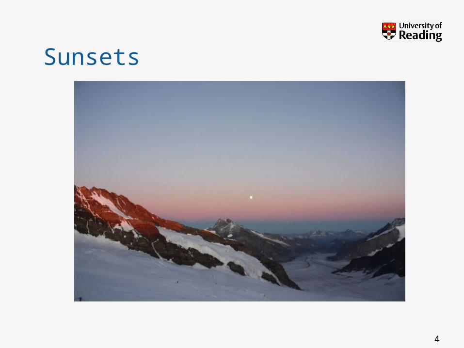
Sunsets
4
Introduction
• Introduction
• Assessment of the consistency of water vapour lines intensities in recent HITRAN databases
• Towards an absolute calibration
• Water Profile for Jungfraujoch
• Future work
5
ASSESSMENT OF THE CONSISTENCY OF WATER VAPOUR LINES INTENSITIES IN RECENT HITRAN DATABASES 6
Consistency Assessment
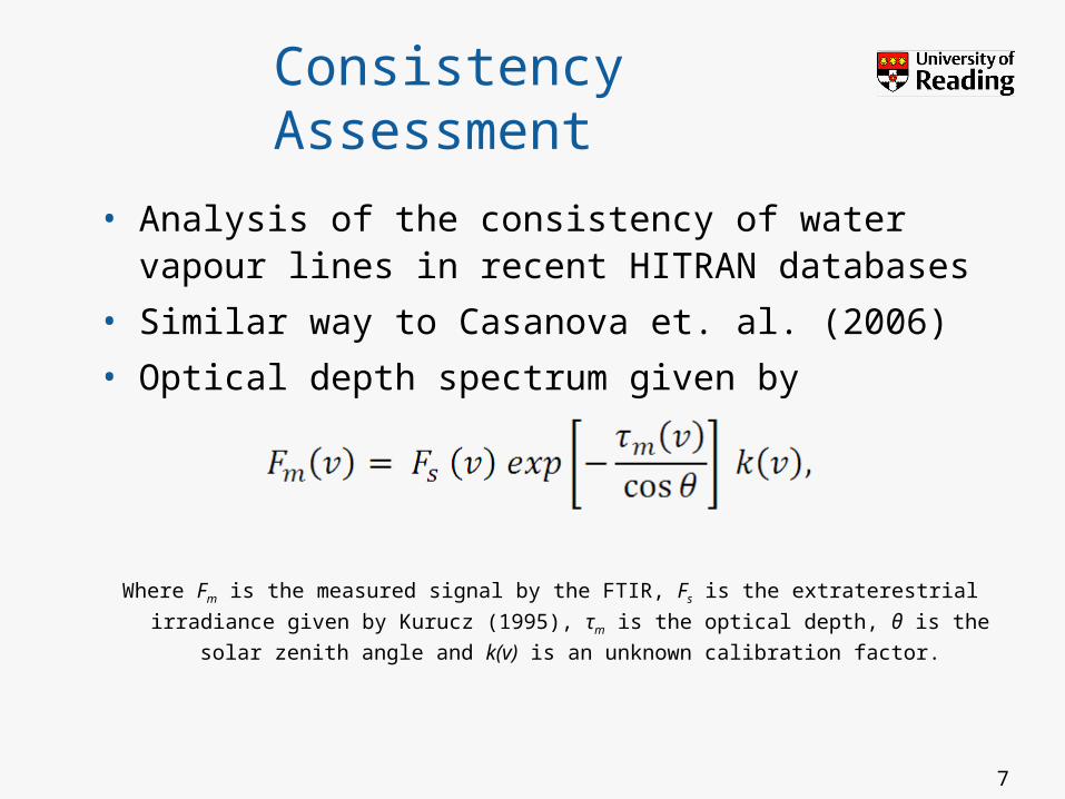
• Analysis of the consistency of water vapour lines in recent HITRAN databases
• Similar way to Casanova et. al. (2006)
• Optical depth spectrum given by
Where Fm is the measured signal by the FTIR, Fs is the extraterestrial irradiance given
by Kurucz (1995), τm is the optical depth, θ is the solar zenith angle and k(v) is an
unknown calibration factor.
7
Consistency Assessment
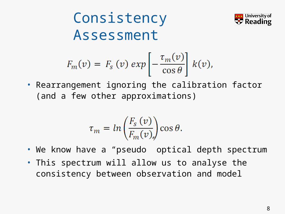
• Rearrangement ignoring the calibration factor (and a few other approximations)
• We know have a “pseudo” optical depth spectrum
• This spectrum will allow us to analyse the consistency between observation and model
8
Consistency Assessment
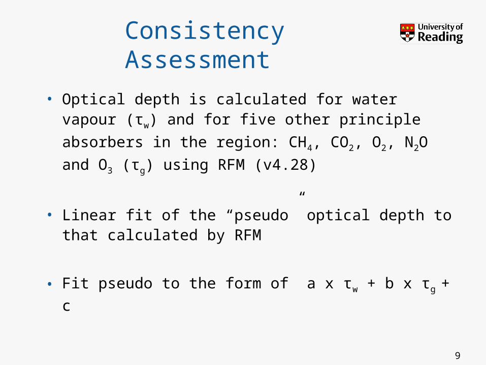
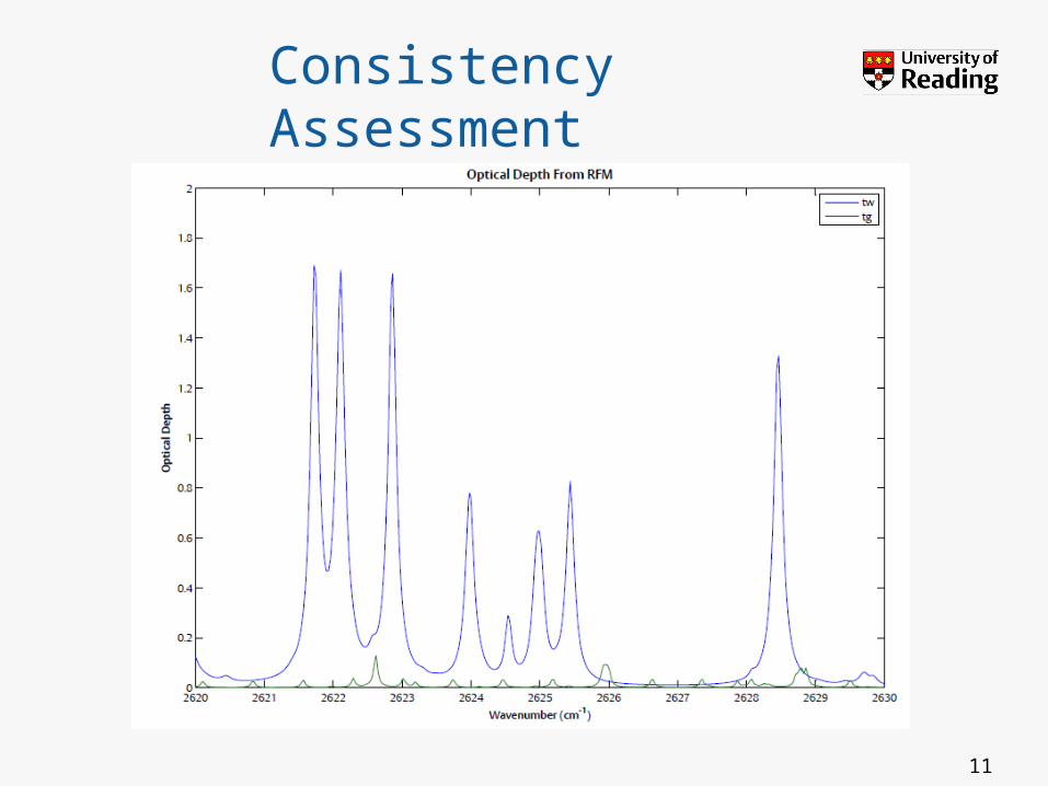
• Optical depth is calculated for water vapour (τw)
and for five other principle absorbers in the region: CH4, CO2, O2, N2O and O3 (τg) using RFM
(v4.28)
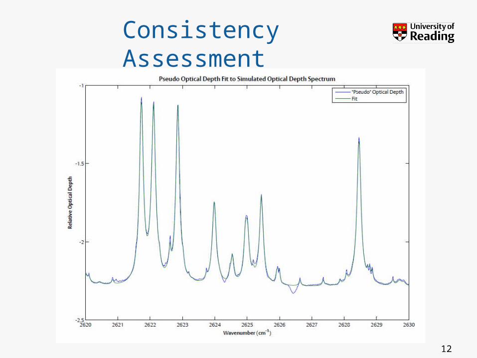
• Linear fit of the “pseudo” optical depth to that calculated by RFM
• Fit pseudo to the form of a x τw + b x τg + c
9
Consistency Assessment
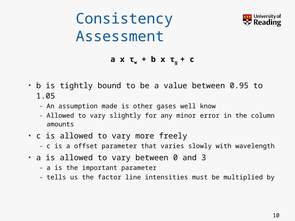
a x τw + b x τg + c
• b is tightly bound to be a value between 0.95 to 1.05– An assumption made is other gases well know– Allowed to vary slightly for any minor error in the column
amounts
• c is allowed to vary more freely– c is a offset parameter that varies slowly with wavelength
• a is allowed to vary between 0 and 3– a is the important parameter– tells us the factor line intensities must be multiplied by
10
Consistency Assessment
11
Consistency Assessment
12
Consistency Assessment
13
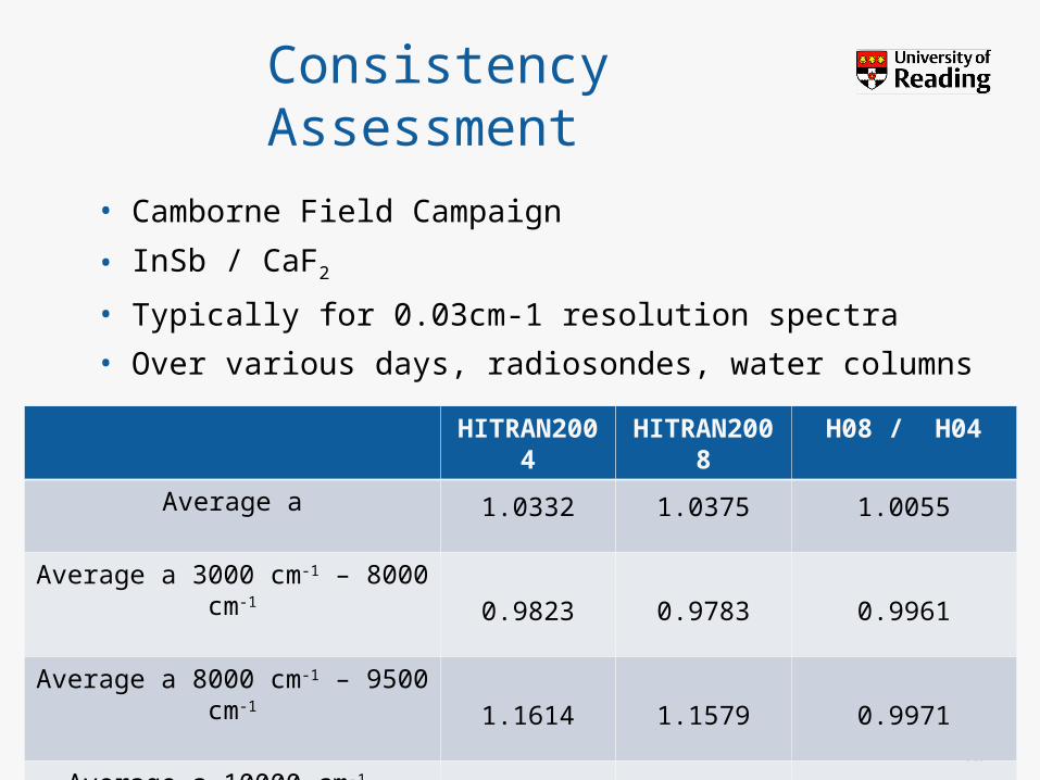
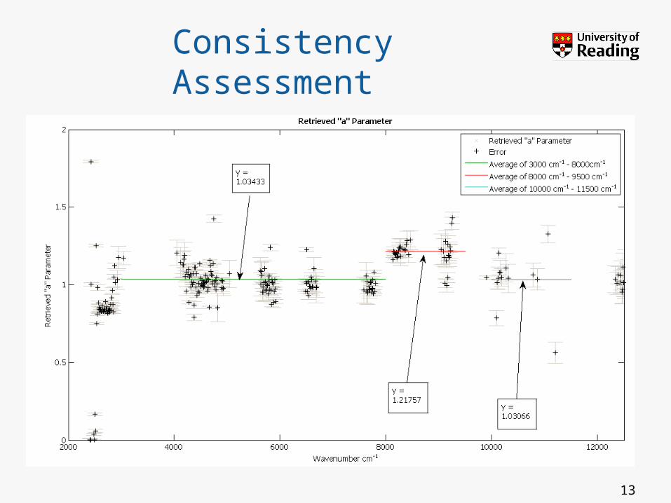
Consistency Assessment
• Camborne Field Campaign
• InSb / CaF2
• Typically for 0.03cm-1 resolution spectra
• Over various days, radiosondes, water columns
14
HITRAN2004
HITRAN2008
H08 / H04
Average a 1.0332 1.0375 1.0055
Average a 3000 cm-1 – 8000 cm-1 0.9823 0.9783 0.9961
Average a 8000 cm-1 – 9500 cm-1 1.1614 1.1579 0.9971
Average a 10000 cm-1 - 11500 cm-1 0.9560 0.9762 1.0233
Consistency Assessment
15
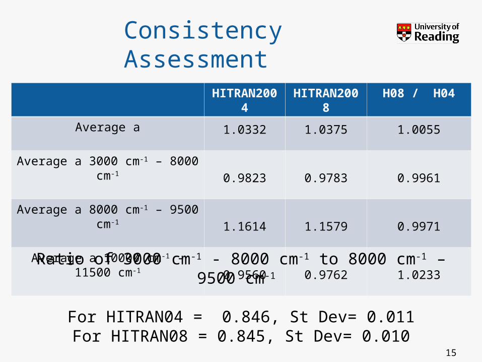
HITRAN2004
HITRAN2008
H08 / H04
Average a 1.0332 1.0375 1.0055
Average a 3000 cm-1 – 8000 cm-1 0.9823 0.9783 0.9961
Average a 8000 cm-1 – 9500 cm-1 1.1614 1.1579 0.9971
Average a 10000 cm-1 - 11500 cm-1 0.9560 0.9762 1.0233
Ratio of 3000 cm-1 - 8000 cm-1 to 8000 cm-1 – 9500 cm-1
For HITRAN04 = 0.846, St Dev= 0.011For HITRAN08 = 0.845, St Dev= 0.010
Consistency Assessment
• Camborne Field Campaign
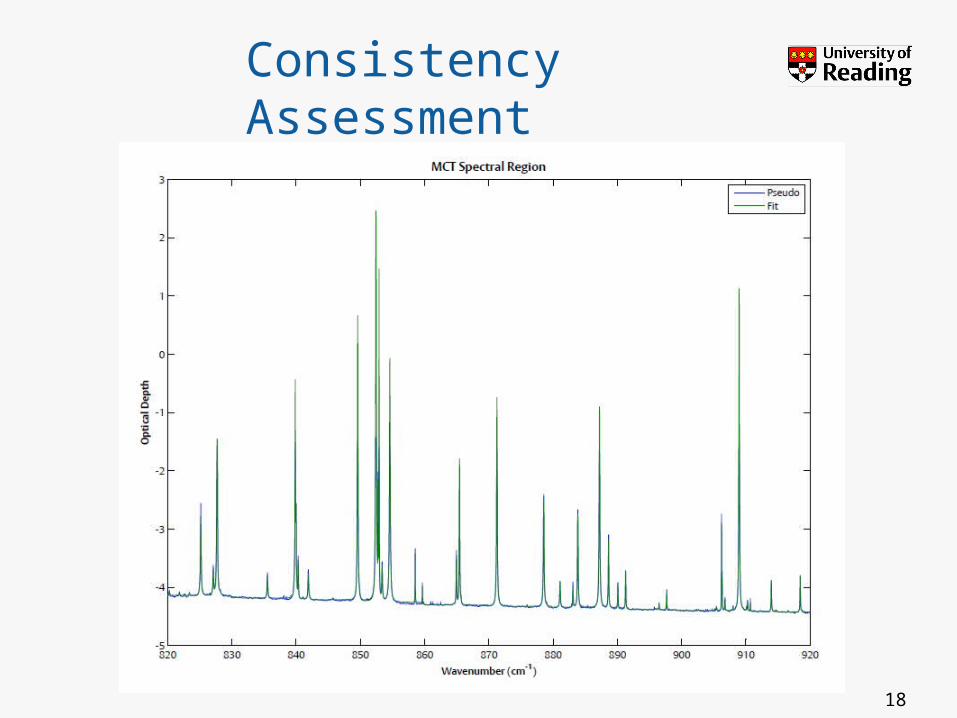
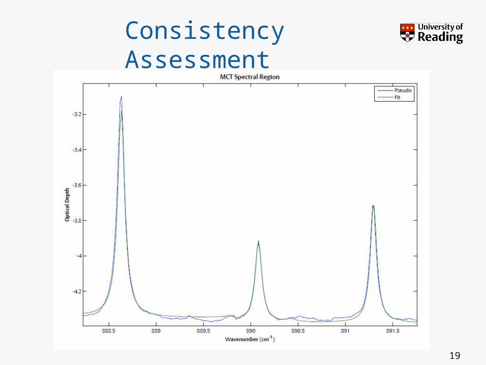
• MCT / KBr
• Problems!
• Fit appears to be good...
• But scaling factor required for water vapour lines feels wrong
• Typical “a” value ~ 0.7
16
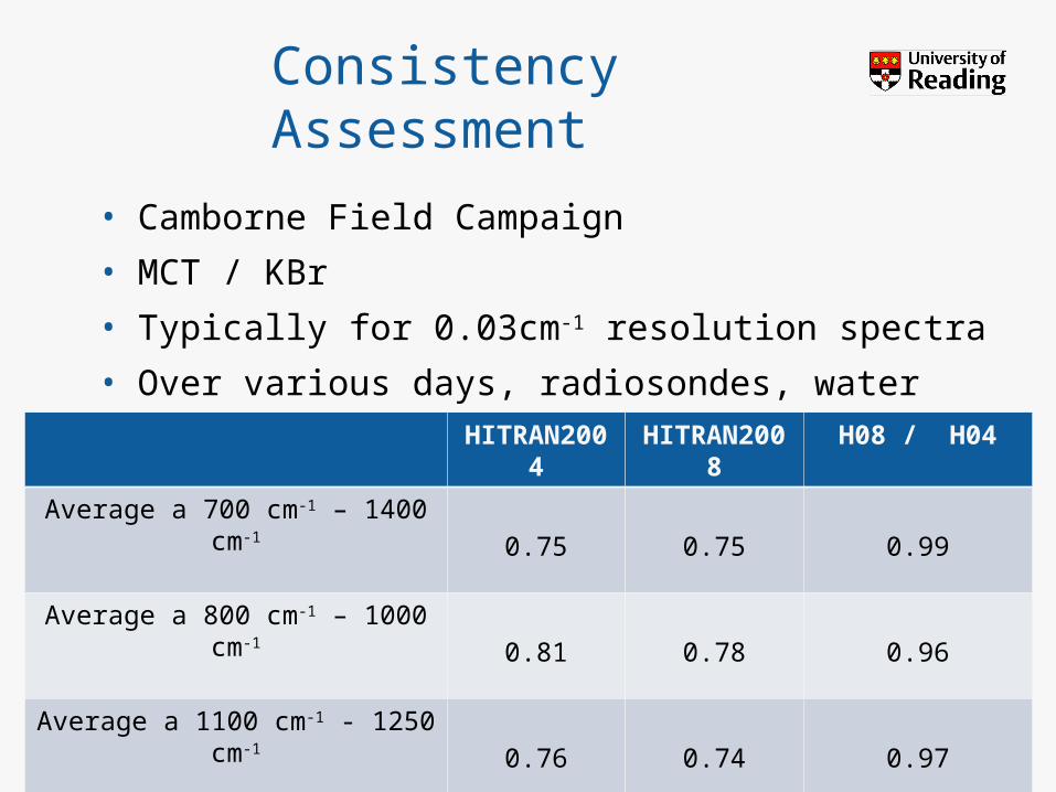
Consistency Assessment
• Camborne Field Campaign
• MCT / KBr
• Typically for 0.03cm-1 resolution spectra
• Over various days, radiosondes, water columns
17
HITRAN2004
HITRAN2008
H08 / H04
Average a 700 cm-1 – 1400 cm-1 0.75 0.75 0.99
Average a 800 cm-1 – 1000 cm-1 0.81 0.78 0.96
Average a 1100 cm-1 - 1250 cm-1 0.76 0.74 0.97
Consistency Assessment
18
Consistency Assessment
19
Consistency Assessment
20
TOWARDS AN ABSOLUTE CALIBRATION
21
Towards an Absolute Calibration
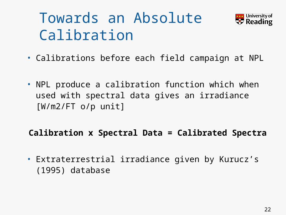
• Calibrations before each field campaign at NPL
• NPL produce a calibration function which when used with spectral data gives an irradiance [W/m2/FT o/p unit]
Calibration x Spectral Data = Calibrated Spectra
• Extraterrestrial irradiance given by Kurucz’s (1995) database
22
Towards an Absolute Calibration
23
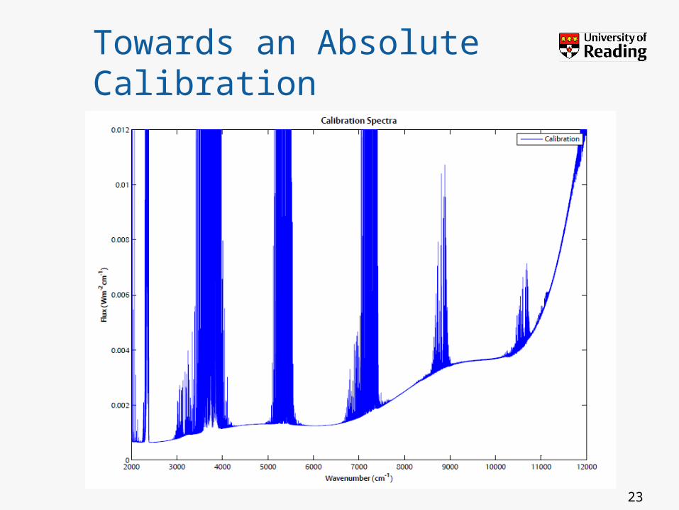
Towards an Absolute Calibration
24
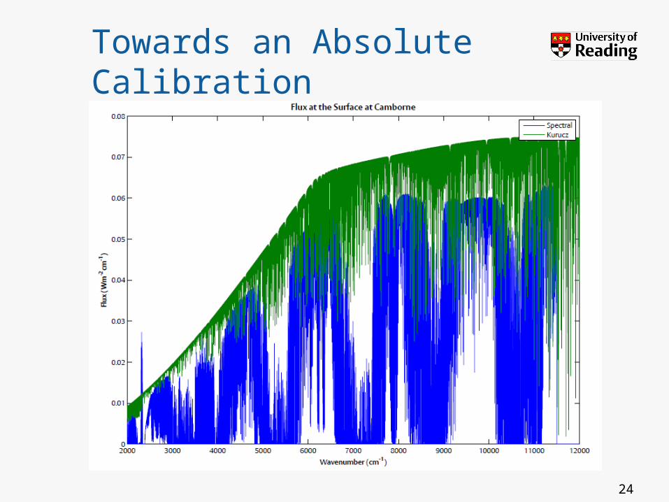
Towards an Absolute Calibration
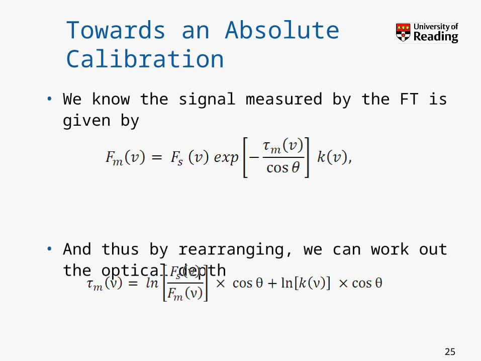
• We know the signal measured by the FT is given by
• And thus by rearranging, we can work out the optical depth
25
Towards an Absolute Calibration
26
Towards an Absolute Calibration
27
Towards an Absolute Calibration
28
Towards an Absolute Calibration
29
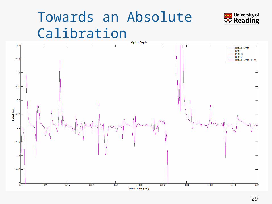
Towards an Absolute Calibration
• Microtops II Sunphotometer
• 13/08/2008
• AOT380 = 0.465, AOT440 = 0.486, AOT675 = 0.577, AOT936 = 0.705, AOT1020 = 0.608
• Campaign Average
• AOT380 = 0.22, AOT440 = 0.17, AOT675 = 0.12, AOT936 = 0.09, AOT1020 = 0.08
30
Towards an Absolute Calibration
31
Towards an Absolute Calibration
32

WATER PROFILE FOR JUNGFRAUJOCH
33
Water Profile for Jungfraujoch
34
• Radiosonde (Payerne)
• Dropsonde (FAAM)
• FAAM Aircraft
• GPS IWV
• ECMWF Forecast Fields
• STARTWAVE Database, University of Bern– GPS Water Vapour– Column Water from Payerne Radiosonde
Water Profile for Jungfraujoch
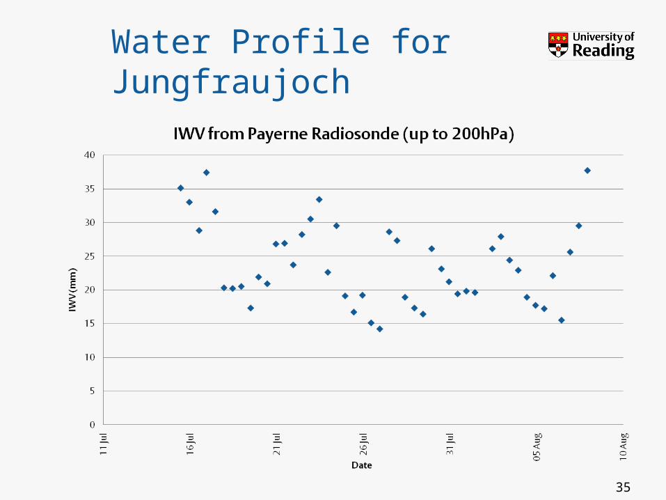
35
Water Profile for Jungfraujoch
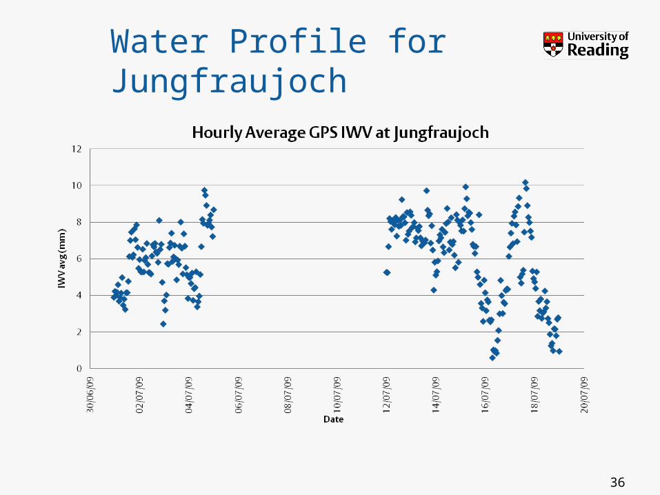
36
Water Profile for Jungfraujoch
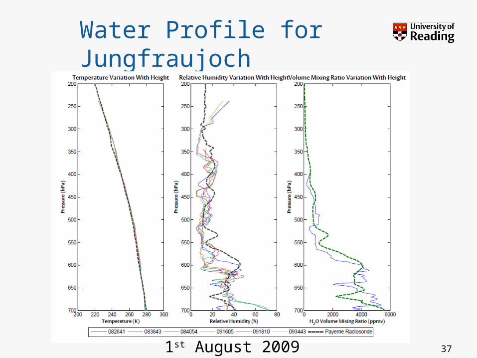
371st August 2009

FUTURE WORK
38
Future Work• Analysis of the consistency of water vapour lines in
recent HITRAN databases– Any improvements to MCT fit possible?– Repeat this style analysis for Jungfraujoch– Try with new ACE-FTS extraterrestrial line list (Hase et. al, JQSRT
2009)
• Absolute Calibration– Account for difference between calibrated spectra and
extraterrestrial irradiance (in atmospheric windows)– Use Reading’s RFM + DISORT Code
• Water Profile for Jungfraujoch– Continued work in this area
• Questions?
39


![Safeguarding/Child Protection Policy - Thomas Tallis School · 4. Thomas Tallis Safeguarding Structures [pg 11-20] There are four key dimensions to Tallis Safeguarding Structures](https://static.fdocuments.net/doc/165x107/5f0c755b7e708231d43580e7/safeguardingchild-protection-policy-thomas-tallis-4-thomas-tallis-safeguarding.jpg)