Causal modelling based on bayesian networks for ...cdn.intechweb.org/pdfs/11956.pdf · Causal...

Causal modelling based on bayesian networks for preliminary design of buildings 293

Causal modelling based on bayesian networks for preliminary design of buildings

Berardo Naticchia and Alessandro Carbonari

X

Causal modelling based on bayesian networks for preliminary design of buildings

Berardo Naticchia and Alessandro Carbonari

Università Politecnica delle Marche, DACS department, Division of Building Construction (www.dacs-bc.univpm.it)

via delle Brecce Bianche, 60131 Ancona, Italy

1. Introduction

The adoption of innovative technologies in construction is sometimes difficult, due to the lack of adequate knowledge to properly estimate and size such systems in the professional environment. Moreover, the lack of proper simulation programs for the preliminary design of buildings which integrate the new technologies prevents the application of these systems to the contemporary construction market, often producing higher costs and less efficient buildings. Despite the recognized validity of several new technological solutions through extended experimentation, and the numerous advances that are being obtained each year, only a small percentage of this technology is being applied to the erection of buildings. This can be explained by the fact that professional architects prefer to adopt standard techniques that they can control rather than try to apply new systems with a high risk of failure, which require assistance from technology experts in order to help architects arrive at their design choices. The best way to overcome these limitations, while fostering wide and fast spread of recently developed technologies on the market, would be to provide professional designers with friendly and reliable simulation tools to help architects discern the best configuration during the conceptual phase of buildings which are to be equipped with these new solutions. In particular, Bayesian Networks will be shown to be a suitable tool for developing multi-criteria decision software programs, given their ease of use and flexibility. In fact, they are able to deal with the difficulty underlying even complex phenomena, by means of an explicit causal framework that links the variables affecting the system. In addition, they can be learned from the same raw data that researchers collect from experiments or advanced simulation tools (e.g. finite difference or finite element methods), automatically giving back accurate estimations to professionals, who in this way do not need to become involved in the use of complex and time consuming simulation programs, like the ones adopted by technology developers. In addition, Bayesian Networks based models can implement decisional functions which are more suitable and quicker than parametric analyses for rough sizing purposes.

18

www.intechopen.com

Bayesian Network294

Even though the Bayesian approach is very powerful, the best methodology to be moulded for its implementation needs to be carefully evaluated, because it must take into account several variables, mainly related to:

- how to build the probabilistic framework relative to complex phenomena involving hundreds of variables linked by non-linear relationships;

- how to use raw data coming from experiments or advanced simulation results to learn conditional probability tables among variables;

- how to validate the model under development. In this chapter a methodology to build a reliable Bayesian model integrating both experimental data and prior knowledge is shown. It is expected to act as a preliminary simulation tool that is a lean and fast way to perform rough sizing, leaving the task of more accurate and time consuming forecasts to the following design stages. Finally, its application to a practical case study for the design of glazed saddlebacked roofpond equipped buildings is taken as an example to show how this multi-criteria decision Bayesian model may be used to assist designers in the problems dealt with by architects during the preliminary stage of design.

2. State of the art

Despite the great potential and flexibility offered by the use of Bayesian Networks, as detailed in the following section 2.1, their application to building design must respond to some basic methodological precautions, which will be indicated in subsection 2.2.

2.1 Scientific background on Bayesian Networks Bayesian networks can be extracted from the knowledge of experts, using a method called causal mapping: it is applied in the context of an information technology outsourcing decision (Nadkarni and Shenoy, 2004). Mathematical models can also be translated into qualitative patterns (Lucas, 2005), in order to infer conditional relations and the graphical structure of the network. Their application has been tested in many areas. Bayesian Networks are used for the management of areas affected by salinity, and they offer the possibility to trade off different kinds of knowledge, like observed data, expert knowledge and results from simulations (Sadoddin et al., 2005). It has been demonstrated that they are able to evaluate the influence of management actions on different aspects of the model framework, such as biophysical, social and economic issues. Bayesian Networks are also applied to study the impact of design, manufacturing and operational decisions relative to oil drill platforms and to the external environment (Zhu et al., 2003). Other applications are known in the field of process monitoring and root cause analysis of complex industrial systems (Weidl et al., 2005). A methodology to be applied in the field of software architectural design, to obtain decisions regarding the adoption or rejection of the best alternative from a web of complex and often uncertain information, has also been proposed (Zhang et al., 2005). The high flexibility of Bayesian Networks has also been shown by (Van Truong et al., 2009), where subjective knowledge, collected by means of questionnaire surveys with experts, was collected to build a network quantifying the most likely causes for delays in construction. Other research is also being carried out in the field of automatic parameter learning in the difficult case of incomplete datasets or sparse data (Wenhui et al., 2009). Bayesian models

also have important properties including the possibility to arrive at decisions, which is critical in many fields, like maintenance processes (Zhiqiang et al., 2008): the networks can be developed from past data about failures and can then be used to obtain decisions, based on the probability of occurrence of future damaging events. Many attempts have also been made in the field of automatic learning Bayesian Networks, whose final purpose would be to provide a machine learning process that finds the network's structure and its associated parameters, which best fit any available dataset (Lauría et al., 2007). However this cannot work properly when data of different kinds are available and they must be put together to develop the final model.

2.2 Advances obtained with respect to the state of the art To the authors’ knowledge, there are no systematic analyses concerning the applicability of Bayesian Networks to the preliminary design stage of innovative buildings, although it is well known that architects involved in this task must cope with a multi-criteria decision making process in order to reason about environmental, cost analysis, structural, aesthetic and other issues (Brouchlaghem, 2000). The software programs which are currently available on the market are mainly based on the numerical solution of complex analytical models. Although accurate and sometimes time-saving, they leave the final choice for the optimization of performance to the designer’s intuition. In fact, an interesting first advance in this direction was pursued by testing Object Oriented models in the housing construction process: the opportunity to visualize and manage together many aspects of this process was appreciated (Harish et al., 2008). Indeed, the possibility to reason from uncertain inputs and to include long-term consequences for each scenario, makes Bayesian tools suitable for use in the early stage of preliminary design, when there is not a complete knowledge of the system and its boundary conditions. The procedure proposed in this chapter is mainly intended to show how to use Bayesian models for building reliable and easy to use simulation tools, which can integrate several types of knowledge coming from different sources into a single probabilistic framework. In addition, this methodology exploits the tool of Object Oriented Bayesian Networks, shortened to OOBNs (Koller et al., 1997), which also helps deal with new technologies which have intrinsic complexity (e.g. many variables interacting according to non-linear relationships) that is a well known challenge for those involved in modelling. Furthermore, they provide an explicit representation of the causal framework that links the variables affecting the system, through which a designer can analyze, criticize and then improve the preliminary project; in order to apply it, he/she needs only know the performance to be obtained and the input data. As regards the specific case of roofponds, presented as a demonstration at the end of this chapter, current approaches proposed by researchers are suitable for executing parametric studies or for verifying thermal performance when boundary conditions are known. Instead, the model developed in the following is able to automatically predict the thermal behaviour of roofpond buildings using only rough input data, which is typical of the preliminary stage of design. This model reasons in a way similar to that adopted by expert designers when detailed data about the new construction are not available, and a heuristic method must be used to describe the system from a functional point of view, inferring the best choice for future design.

www.intechopen.com


Even though the Bayesian approach is very powerful, the best methodology to be moulded for its implementation needs to be carefully evaluated, because it must take into account several variables, mainly related to:

- how to build the probabilistic framework relative to complex phenomena involving hundreds of variables linked by non-linear relationships;

- how to use raw data coming from experiments or advanced simulation results to learn conditional probability tables among variables;

- how to validate the model under development. In this chapter a methodology to build a reliable Bayesian model integrating both experimental data and prior knowledge is shown. It is expected to act as a preliminary simulation tool that is a lean and fast way to perform rough sizing, leaving the task of more accurate and time consuming forecasts to the following design stages. Finally, its application to a practical case study for the design of glazed saddlebacked roofpond equipped buildings is taken as an example to show how this multi-criteria decision Bayesian model may be used to assist designers in the problems dealt with by architects during the preliminary stage of design.

2. State of the art

Despite the great potential and flexibility offered by the use of Bayesian Networks, as detailed in the following section 2.1, their application to building design must respond to some basic methodological precautions, which will be indicated in subsection 2.2.

2.1 Scientific background on Bayesian Networks Bayesian networks can be extracted from the knowledge of experts, using a method called causal mapping: it is applied in the context of an information technology outsourcing decision (Nadkarni and Shenoy, 2004). Mathematical models can also be translated into qualitative patterns (Lucas, 2005), in order to infer conditional relations and the graphical structure of the network. Their application has been tested in many areas. Bayesian Networks are used for the management of areas affected by salinity, and they offer the possibility to trade off different kinds of knowledge, like observed data, expert knowledge and results from simulations (Sadoddin et al., 2005). It has been demonstrated that they are able to evaluate the influence of management actions on different aspects of the model framework, such as biophysical, social and economic issues. Bayesian Networks are also applied to study the impact of design, manufacturing and operational decisions relative to oil drill platforms and to the external environment (Zhu et al., 2003). Other applications are known in the field of process monitoring and root cause analysis of complex industrial systems (Weidl et al., 2005). A methodology to be applied in the field of software architectural design, to obtain decisions regarding the adoption or rejection of the best alternative from a web of complex and often uncertain information, has also been proposed (Zhang et al., 2005). The high flexibility of Bayesian Networks has also been shown by (Van Truong et al., 2009), where subjective knowledge, collected by means of questionnaire surveys with experts, was collected to build a network quantifying the most likely causes for delays in construction. Other research is also being carried out in the field of automatic parameter learning in the difficult case of incomplete datasets or sparse data (Wenhui et al., 2009). Bayesian models

also have important properties including the possibility to arrive at decisions, which is critical in many fields, like maintenance processes (Zhiqiang et al., 2008): the networks can be developed from past data about failures and can then be used to obtain decisions, based on the probability of occurrence of future damaging events. Many attempts have also been made in the field of automatic learning Bayesian Networks, whose final purpose would be to provide a machine learning process that finds the network's structure and its associated parameters, which best fit any available dataset (Lauría et al., 2007). However this cannot work properly when data of different kinds are available and they must be put together to develop the final model.

2.2 Advances obtained with respect to the state of the art To the authors’ knowledge, there are no systematic analyses concerning the applicability of Bayesian Networks to the preliminary design stage of innovative buildings, although it is well known that architects involved in this task must cope with a multi-criteria decision making process in order to reason about environmental, cost analysis, structural, aesthetic and other issues (Brouchlaghem, 2000). The software programs which are currently available on the market are mainly based on the numerical solution of complex analytical models. Although accurate and sometimes time-saving, they leave the final choice for the optimization of performance to the designer’s intuition. In fact, an interesting first advance in this direction was pursued by testing Object Oriented models in the housing construction process: the opportunity to visualize and manage together many aspects of this process was appreciated (Harish et al., 2008). Indeed, the possibility to reason from uncertain inputs and to include long-term consequences for each scenario, makes Bayesian tools suitable for use in the early stage of preliminary design, when there is not a complete knowledge of the system and its boundary conditions. The procedure proposed in this chapter is mainly intended to show how to use Bayesian models for building reliable and easy to use simulation tools, which can integrate several types of knowledge coming from different sources into a single probabilistic framework. In addition, this methodology exploits the tool of Object Oriented Bayesian Networks, shortened to OOBNs (Koller et al., 1997), which also helps deal with new technologies which have intrinsic complexity (e.g. many variables interacting according to non-linear relationships) that is a well known challenge for those involved in modelling. Furthermore, they provide an explicit representation of the causal framework that links the variables affecting the system, through which a designer can analyze, criticize and then improve the preliminary project; in order to apply it, he/she needs only know the performance to be obtained and the input data. As regards the specific case of roofponds, presented as a demonstration at the end of this chapter, current approaches proposed by researchers are suitable for executing parametric studies or for verifying thermal performance when boundary conditions are known. Instead, the model developed in the following is able to automatically predict the thermal behaviour of roofpond buildings using only rough input data, which is typical of the preliminary stage of design. This model reasons in a way similar to that adopted by expert designers when detailed data about the new construction are not available, and a heuristic method must be used to describe the system from a functional point of view, inferring the best choice for future design.

www.intechopen.com

Bayesian Network296

3. Developing complex Bayesian Network models

3.1 Brief overview on Bayesian Networks The main asset of Bayesian Networks lays in the integration of qualitative physical patterns (Boborow, 1984) and computational algorithms elaborated in the field of artificial intelligence (Jensen, 2000) in order to create an intelligent support tool. The main utility of Bayesian Networks consists in the possibility to combine typical results from macroscopic and microscopic analyses (Naticchia et al., 2001). Combining the two approaches, designers have the possibility to perform a trial approach also considering very detailed numerical results in order to reach a higher reliability. Over the last decade, Bayesian Networks (also called belief bayesian networks or causal probabilistic networks) have dominated the field of reasoning under uncertainty, thanks to the ability of such expert models to deal with incomplete or uncertain information (Pearl, 1988; Korb and Nicholson, 2004). Bayesian Networks consist of two parts: a graphical model and an underlying conditional probability distribution. The graphical model is represented by a directed acyclic graph (DAG), whose nodes represent random variables, which are linked by arcs, corresponding to causal relationships with the previous ones. Each variable may take two or more possible states, of both numerical and label types. An arc from a variable A to another variable B denotes, in the general case, that A causes B. Using the standard terminology, A is said to be a parent of B (which is its child). The strength of that relationship is quantified by conditional probability tables (Wonnacott and Wonnacott, 1990), where the probability to observe each state of any child variable is given with respect to all combinations of its parents’ states; in our example it would be generally billed P(b|a), where A is conditionally independent of any variable of the domain that is not its parent, and “a” defines a generic state for variable A. The same holds for variable B. Thus we can obtain a conditional probability distribution over every domain, where the state of each variable can be determined by the knowledge only of the state of its parents, and the joint probability of a set of variables E can be computed applying the “chain rule” (Pearl, 1988): 1121 |...|,..., EPEEPEparentsEPEEPEP nnn (1)

Eq. (1) simplifies the computational process considerably, and it is also the first main feature of Bayesian Networks. In other words, the joint probability of any combination of variables E is given by the product between the variable En, given any sub-set of variables that includes only the parents of En, and any sub-set of variables that are simply ancestors of En, given the conditional probabilities of their parents. Thus the complete specification of any joint probability distribution does not require an absurdly huge database as is the case when every variable is considered to be dependent on the others (Charniak, 1991). Secondly, the Bayesian explicit graphical representation also provides a clear understanding of the qualitative relationships among variables, allowing the user to reason about their causal correlations. In addition, every node of a Bayesian Network can be conditioned with new information via a flow of information through the network. The probability of a set of “query” nodes is computed given the evidence on other nodes for which observations are already available. Furthermore, parameter updating is supported for any direction of reasoning: from causes

to consequences (“predictive” reasoning) or from consequences to causes (“diagnostic” reasoning). This advantage derives from the application of the “Bayes Theorem”:

ePHPHePeHP || (2)

where H is the variable with unknown probability distribution; e is the set of variables for which evidence has been obtained. Finally, Bayesian Networks have the important capability to update it from new evidence: this can be formulated by gradually substituting the prior probability distribution P(H) with P(H|en), that is the probability distribution of H conditioned upon a set of old evidence en. Similarly P(e|H) becomes P(e|en,H), and P(e) becomes P(e|en):

n

nnn eeP

eHPHeePeeHP|

|,|,| (3)

3.2 Building the graphical structure The three basic reference modules of elementary graphical structures are provided in Fig. 1 (Pearl, 1988): given the case of Fig. 1-a, the probability of C, given B, is exactly the same as the probability of C, given A and B. Therefore A and C are conditionally independent: that structure is called a causal chain. The common causes structure in Fig. 1-b is slightly more complex: if there is no evidence or information about B, then learning the probability distribution of A or C will change the probability distribution of the unknown variable between A or C; in the opposite case, when B is given, the knowledge of A or C will not change the probability distribution of the other. The last common effects structure in Fig. 1-c, represents the situation where an effect has two causes: the parents are marginally independent, but become dependent given information about the common effect. While building any causal structure to develop a probabilistic model before validation, this must be compared with the elementary networks in Fig. 1, in order to verify that any conditional independence stated by the causal model really corresponds to the meaning assigned by the corresponding basic reference structure.

a)

b) c) Fig. 1. Elementary networks for conditional independence assumptions.

3.3 Object Oriented Bayesian Networks Probabilistic causal networks to model complex physical phenomena are expected to be made up of several elementary networks (each of them devoted to modelling a part of the whole process), and assembled through the use of Object Oriented Bayesian Networks (OOBNs). This functionality is particularly useful to provide a hierarchical description of complex technology systems, because it breaks down the whole domain into single units or

www.intechopen.com


3. Developing complex Bayesian Network models

3.1 Brief overview on Bayesian Networks The main asset of Bayesian Networks lays in the integration of qualitative physical patterns (Boborow, 1984) and computational algorithms elaborated in the field of artificial intelligence (Jensen, 2000) in order to create an intelligent support tool. The main utility of Bayesian Networks consists in the possibility to combine typical results from macroscopic and microscopic analyses (Naticchia et al., 2001). Combining the two approaches, designers have the possibility to perform a trial approach also considering very detailed numerical results in order to reach a higher reliability. Over the last decade, Bayesian Networks (also called belief bayesian networks or causal probabilistic networks) have dominated the field of reasoning under uncertainty, thanks to the ability of such expert models to deal with incomplete or uncertain information (Pearl, 1988; Korb and Nicholson, 2004). Bayesian Networks consist of two parts: a graphical model and an underlying conditional probability distribution. The graphical model is represented by a directed acyclic graph (DAG), whose nodes represent random variables, which are linked by arcs, corresponding to causal relationships with the previous ones. Each variable may take two or more possible states, of both numerical and label types. An arc from a variable A to another variable B denotes, in the general case, that A causes B. Using the standard terminology, A is said to be a parent of B (which is its child). The strength of that relationship is quantified by conditional probability tables (Wonnacott and Wonnacott, 1990), where the probability to observe each state of any child variable is given with respect to all combinations of its parents’ states; in our example it would be generally billed P(b|a), where A is conditionally independent of any variable of the domain that is not its parent, and “a” defines a generic state for variable A. The same holds for variable B. Thus we can obtain a conditional probability distribution over every domain, where the state of each variable can be determined by the knowledge only of the state of its parents, and the joint probability of a set of variables E can be computed applying the “chain rule” (Pearl, 1988): 1121 |...|,..., EPEEPEparentsEPEEPEP nnn (1)

Eq. (1) simplifies the computational process considerably, and it is also the first main feature of Bayesian Networks. In other words, the joint probability of any combination of variables E is given by the product between the variable En, given any sub-set of variables that includes only the parents of En, and any sub-set of variables that are simply ancestors of En, given the conditional probabilities of their parents. Thus the complete specification of any joint probability distribution does not require an absurdly huge database as is the case when every variable is considered to be dependent on the others (Charniak, 1991). Secondly, the Bayesian explicit graphical representation also provides a clear understanding of the qualitative relationships among variables, allowing the user to reason about their causal correlations. In addition, every node of a Bayesian Network can be conditioned with new information via a flow of information through the network. The probability of a set of “query” nodes is computed given the evidence on other nodes for which observations are already available. Furthermore, parameter updating is supported for any direction of reasoning: from causes

to consequences (“predictive” reasoning) or from consequences to causes (“diagnostic” reasoning). This advantage derives from the application of the “Bayes Theorem”:

ePHPHePeHP || (2)

where H is the variable with unknown probability distribution; e is the set of variables for which evidence has been obtained. Finally, Bayesian Networks have the important capability to update it from new evidence: this can be formulated by gradually substituting the prior probability distribution P(H) with P(H|en), that is the probability distribution of H conditioned upon a set of old evidence en. Similarly P(e|H) becomes P(e|en,H), and P(e) becomes P(e|en):

n

nnn eeP

eHPHeePeeHP|

|,|,| (3)

3.2 Building the graphical structure The three basic reference modules of elementary graphical structures are provided in Fig. 1 (Pearl, 1988): given the case of Fig. 1-a, the probability of C, given B, is exactly the same as the probability of C, given A and B. Therefore A and C are conditionally independent: that structure is called a causal chain. The common causes structure in Fig. 1-b is slightly more complex: if there is no evidence or information about B, then learning the probability distribution of A or C will change the probability distribution of the unknown variable between A or C; in the opposite case, when B is given, the knowledge of A or C will not change the probability distribution of the other. The last common effects structure in Fig. 1-c, represents the situation where an effect has two causes: the parents are marginally independent, but become dependent given information about the common effect. While building any causal structure to develop a probabilistic model before validation, this must be compared with the elementary networks in Fig. 1, in order to verify that any conditional independence stated by the causal model really corresponds to the meaning assigned by the corresponding basic reference structure.

a)

b) c) Fig. 1. Elementary networks for conditional independence assumptions.

3.3 Object Oriented Bayesian Networks Probabilistic causal networks to model complex physical phenomena are expected to be made up of several elementary networks (each of them devoted to modelling a part of the whole process), and assembled through the use of Object Oriented Bayesian Networks (OOBNs). This functionality is particularly useful to provide a hierarchical description of complex technology systems, because it breaks down the whole domain into single units or

www.intechopen.com

Bayesian Network298

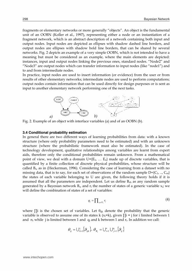
fragments or elementary networks or more generally “objects”. An object is the fundamental unit of an OOBN (Koller et al., 1997), representing either a node or an instantiation of a fragment network, which is an abstract description of a network containing both input and output nodes. Input nodes are depicted as ellipses with shadow dashed line borders, and output nodes are ellipses with shadow bold line borders, that can be shared by several networks. Fig. 2 depicts an example of a very simple OOBN, which is not intended to have a meaning but must be considered as an example, where the main elements are depicted: instances, input and output nodes linking the previous ones, standard nodes. “Node2” and “Node3” are output nodes which can transfer information to input nodes (like “node1”) and to and from intermediate nodes. In practice, input nodes are used to insert information (or evidence) from the user or from results of other elementary networks; intermediate nodes are used to perform computations; output nodes contain information that can be used directly for design purposes or is sent as input to another elementary network performing one of the next tasks.

a) b) Fig. 2. Example of an object with interface variables (a) and of an OOBN (b).

3.4 Conditional probability estimation In general there are two different ways of learning probabilities from data: with a known structure (where only probability parameters need to be estimated) and with an unknown structure (where the probabilistic framework must also be estimated). In the case of technology development, qualitative relationships among variables are learnt from expert aids, therefore only the conditional probabilities remain unknown. From a mathematical point of view, we deal with a domain U={E1, … En} made up of discrete variables, that is quantified by a finite collection of discrete physical probabilities, whose structure will be called Bs, as in (Heckerman, 1996). Considering the case of learning from a dataset with no missing data, that is to say, for each set of observations of the random sample D={C1, .., Cm} the states of each variable belonging to U are given, the following theory holds if it is assumed that all the parameters are independent. Let us define Bsh as any random sample generated by a Bayesian network Bs, and ri the number of states of a generic variable xi; we will define the combination of states of a set of variables:

ilx li rq (4)

where ∏i is the chosen set of variables. Let θijk denote the probability that the generic variable is observed to assume one of its states k (xi=k), given ∏i = j for i limited between 1 and n, while j is limited between 1 and qi and k between 1 and ri. In addition we call: ijk

rkiji 1 , ij

qj

niB

i

s 11

and we suppose that each variable set θij has a Dirichlet distribution: i

ijkr

k

Nijk

hsij cBp

1

1'

,| (5)

where c is a normalization constant, N’ijk are the multinomial parameters of that distribution, limited between 0 and 1, finally ξ is the observed evidence. Eq. (5) can also be expressed in its explicit form using the gamma function Г (Evans et al., 1993):

i

ijkr

k

Nijkr

kk

r

kk

hsij

N

NBp

1

1

1

1 '

'

',| (6)

Thus, if Nijk is the number of observations in the database D in which xi=k and ∏i=j we are able to update that distribution: i

ijkijkr

k

NNijk

hsij cBDp

1

1'

,,| (7)

Eq. (7) is applied to each case belonging to that database. Exploiting the properties of Dirichlet distributions, we can compute the probability that xi=k and ∏i=j in the next case to be seen in the database Cm+1 (but not observed yet) as:

iq

j ijij

ijkijkn

i

hsm NN

NNBDCp

111 '

',,| (8)

where:

ir

kijkij NN

1'' , ir

kijkij NN

1

In the case of missing data in the database D, the “EM learning” algorithm can be applied (Lauritzen, 1995). After learning the probabilities from a database D, it could be necessary to add other information from further empirical data. This can be carried out using the “sequential updating” method, that is a procedure to modify the network parameters over time in order to improve its performance. This method works by modifying the multinomial parameters of the Dirichlet distributions under the assumption of parameter independence. With the term “experience”, we mean quantitative memory which can be based both on quantitative expert judgment and past cases (Spiegelalther and Laurintzen, 1990). For the purpose of learning models relative to the preliminary design of buildings, the prior parameters in the first version of the network can be set with a particular equivalent sample size (by tuning the values N’ijk), after which more data are added using the same procedure, starting from the new equivalent sample size and Dirichlet parameters, independently from

www.intechopen.com


fragments or elementary networks or more generally “objects”. An object is the fundamental unit of an OOBN (Koller et al., 1997), representing either a node or an instantiation of a fragment network, which is an abstract description of a network containing both input and output nodes. Input nodes are depicted as ellipses with shadow dashed line borders, and output nodes are ellipses with shadow bold line borders, that can be shared by several networks. Fig. 2 depicts an example of a very simple OOBN, which is not intended to have a meaning but must be considered as an example, where the main elements are depicted: instances, input and output nodes linking the previous ones, standard nodes. “Node2” and “Node3” are output nodes which can transfer information to input nodes (like “node1”) and to and from intermediate nodes. In practice, input nodes are used to insert information (or evidence) from the user or from results of other elementary networks; intermediate nodes are used to perform computations; output nodes contain information that can be used directly for design purposes or is sent as input to another elementary network performing one of the next tasks.

a) b) Fig. 2. Example of an object with interface variables (a) and of an OOBN (b).

3.4 Conditional probability estimation In general there are two different ways of learning probabilities from data: with a known structure (where only probability parameters need to be estimated) and with an unknown structure (where the probabilistic framework must also be estimated). In the case of technology development, qualitative relationships among variables are learnt from expert aids, therefore only the conditional probabilities remain unknown. From a mathematical point of view, we deal with a domain U={E1, … En} made up of discrete variables, that is quantified by a finite collection of discrete physical probabilities, whose structure will be called Bs, as in (Heckerman, 1996). Considering the case of learning from a dataset with no missing data, that is to say, for each set of observations of the random sample D={C1, .., Cm} the states of each variable belonging to U are given, the following theory holds if it is assumed that all the parameters are independent. Let us define Bsh as any random sample generated by a Bayesian network Bs, and ri the number of states of a generic variable xi; we will define the combination of states of a set of variables:

ilx li rq (4)

where ∏i is the chosen set of variables. Let θijk denote the probability that the generic variable is observed to assume one of its states k (xi=k), given ∏i = j for i limited between 1 and n, while j is limited between 1 and qi and k between 1 and ri. In addition we call: ijk

rkiji 1 , ij

qj

niB

i

s 11

and we suppose that each variable set θij has a Dirichlet distribution: i

ijkr

k

Nijk

hsij cBp

1

1'

,| (5)

where c is a normalization constant, N’ijk are the multinomial parameters of that distribution, limited between 0 and 1, finally ξ is the observed evidence. Eq. (5) can also be expressed in its explicit form using the gamma function Г (Evans et al., 1993):

i

ijkr

k

Nijkr

kk

r

kk

hsij

N

NBp

1

1

1

1 '

'

',| (6)

Thus, if Nijk is the number of observations in the database D in which xi=k and ∏i=j we are able to update that distribution: i

ijkijkr

k

NNijk

hsij cBDp

1

1'

,,| (7)

Eq. (7) is applied to each case belonging to that database. Exploiting the properties of Dirichlet distributions, we can compute the probability that xi=k and ∏i=j in the next case to be seen in the database Cm+1 (but not observed yet) as:

iq

j ijij

ijkijkn

i

hsm NN

NNBDCp

111 '

',,| (8)

where:

ir

kijkij NN

1'' , ir

kijkij NN

1

In the case of missing data in the database D, the “EM learning” algorithm can be applied (Lauritzen, 1995). After learning the probabilities from a database D, it could be necessary to add other information from further empirical data. This can be carried out using the “sequential updating” method, that is a procedure to modify the network parameters over time in order to improve its performance. This method works by modifying the multinomial parameters of the Dirichlet distributions under the assumption of parameter independence. With the term “experience”, we mean quantitative memory which can be based both on quantitative expert judgment and past cases (Spiegelalther and Laurintzen, 1990). For the purpose of learning models relative to the preliminary design of buildings, the prior parameters in the first version of the network can be set with a particular equivalent sample size (by tuning the values N’ijk), after which more data are added using the same procedure, starting from the new equivalent sample size and Dirichlet parameters, independently from

www.intechopen.com

Bayesian Network300

the numerousness of the first dataset. As regards the equivalent sample size relative to the first learning procedure, the larger its size, the greater is the confidence in the previous parameter estimates and the slower the change due to adapting to new data. This technique is also valid with missing data. The procedure described in the next paragraph is intended to provide a generally valid method, to find the optimum ratio between the equivalent sample size and the added empirical database. As further detailed in 4.1, this procedure requires an iterative adaptation of the parameters, until two quality indices of the network are optimized: sensitivity and case-based reasoning. As an alternative, probabilities can be derived by deterministic relations. As required by the subdivision of variables into discrete intervals, this kind of algebra deals with real intervals (Alefeld and Herberg, 1983). In such a case, assuming that [a1, b1), [a2, b2) … [an, bn] are a set of contiguous intervals in the real field, the variables domain will be defined as: nnni pbapbapbaX :,,..,:,,:, 222111 (9) In other words the probability distribution of a generic variable of the Bayesian model will be defined as: nnniii pbaxpbaxpbaxP ,,..,,;, 222111 (10) This kind of interval subdivision will be assigned to each variable, both of the “parent” and “child” type. However, only the distribution of the parent variables is known and not that of the child variables. Subsequently a mathematical expression linking the state of each child to that of their parent variables can be used to compute the probability distribution of child variables (Hugin, 2008): at this juncture, a number of samples within each (bounded) interval of the parents are generated (generally according to the Monte Carlo Simulation method). Each of these samples will result in a “degenerated distribution” for the child node with each distribution corresponding to a given state for the parents. The final distribution assigned to the child node is the average over all the generated distributions. This amounts to counting the number of times a given child state appears when applying deterministic relationships to the generated sample.

4. Causal modelling for the preliminary design of buildings

4.1 Description of the general procedure The general procedure suggested (and applied to a real case in the following) for setting up Bayesian models for the preliminary design of buildings, involves the following steps (Fig. 3): 1. decomposition of all the physical phenomena governing the technology into a set of several simpler processes, which describe their qualitative features through graphical structure representations (linked nodes) and their validation from a semantic point of view; 2. combination of the sub-networks developed on item no. 1 through interface variables into Object Oriented Networks in order to obtain only one whole model; 3. verification of the semantics of this whole model by technology experts, checking that the arrangement aggregation has not determined a lack of meaning;

4. formulation of a simplified release of available analytical methods to work out a first estimation of conditional probabilities; 5. preliminary updating of these conditional probability tables with raw data collected from simulations or field tests; 6. first evaluation of the quality of the network in step no. 5, through sensitivity analyses and case-based validations; 7. iterative refinement of parameters, adding further empirical information, while repeating again items no. 5 and 6. The application of this 7-step procedure provides the following benefits:

1. explicit representation of all the complex phenomena involved in the building’s behaviour through the graphical part of a Bayesian Network;

2. exploitation of both simplified relationships and experimental data to work out reliable (and validated) conditional probability networks;

3. production of a friendly simulation tool, which can act as an expert system in support of professional architects.

Validations in steps 1 and 3 can be performed by comparing the meaning of the qualitative causal relationships represented by the elementary networks in Fig. 1 with the real role played by each variable affecting the technology under development. The first probability learning from deterministic relations in step no. 4, is useful to estimate the parameter N’ijk mentioned in paragraph 3.4 (assessing theoretical knowledge), while the raw data in step no. 5 add further knowledge to estimate the parameters Nijk. Finally, network quality evaluation in steps no. 6 and 7 requires the use of sensitivity analysis and case-based reasoning. In general, any Bayesian network contains a high level of information if it is sensitive to changes in parameters and if it does not produce even probability distributions. For the purpose of model development, the selection among several networks with different values of conditional probabilities is required, each generated from a different probability elicitation, corresponding to a different ratio between theoretical and empirical knowledge. For that purpose, sensitivity to changes in parameters is applied. This method can be exploited in order to find the best ratio between different amounts of experience and theoretical knowledge. The best solution is supposed to be the one giving back the sharpest probability distribution on each variable of interest. Entropy is the metric used to measure the variables’ level of information (in the rest of this paper shortened to LOI): its lowest extreme is zero and corresponds to the maximum level of certainty; therefore the final aim is to minimize entropy. This is defined as (Korb and Nicholson, 2004): kPkPxH

xk2log (11)

being the summation on k carried out for each possible state of the query node.

www.intechopen.com


the numerousness of the first dataset. As regards the equivalent sample size relative to the first learning procedure, the larger its size, the greater is the confidence in the previous parameter estimates and the slower the change due to adapting to new data. This technique is also valid with missing data. The procedure described in the next paragraph is intended to provide a generally valid method, to find the optimum ratio between the equivalent sample size and the added empirical database. As further detailed in 4.1, this procedure requires an iterative adaptation of the parameters, until two quality indices of the network are optimized: sensitivity and case-based reasoning. As an alternative, probabilities can be derived by deterministic relations. As required by the subdivision of variables into discrete intervals, this kind of algebra deals with real intervals (Alefeld and Herberg, 1983). In such a case, assuming that [a1, b1), [a2, b2) … [an, bn] are a set of contiguous intervals in the real field, the variables domain will be defined as: nnni pbapbapbaX :,,..,:,,:, 222111 (9) In other words the probability distribution of a generic variable of the Bayesian model will be defined as: nnniii pbaxpbaxpbaxP ,,..,,;, 222111 (10) This kind of interval subdivision will be assigned to each variable, both of the “parent” and “child” type. However, only the distribution of the parent variables is known and not that of the child variables. Subsequently a mathematical expression linking the state of each child to that of their parent variables can be used to compute the probability distribution of child variables (Hugin, 2008): at this juncture, a number of samples within each (bounded) interval of the parents are generated (generally according to the Monte Carlo Simulation method). Each of these samples will result in a “degenerated distribution” for the child node with each distribution corresponding to a given state for the parents. The final distribution assigned to the child node is the average over all the generated distributions. This amounts to counting the number of times a given child state appears when applying deterministic relationships to the generated sample.

4. Causal modelling for the preliminary design of buildings

4.1 Description of the general procedure The general procedure suggested (and applied to a real case in the following) for setting up Bayesian models for the preliminary design of buildings, involves the following steps (Fig. 3): 1. decomposition of all the physical phenomena governing the technology into a set of several simpler processes, which describe their qualitative features through graphical structure representations (linked nodes) and their validation from a semantic point of view; 2. combination of the sub-networks developed on item no. 1 through interface variables into Object Oriented Networks in order to obtain only one whole model; 3. verification of the semantics of this whole model by technology experts, checking that the arrangement aggregation has not determined a lack of meaning;

4. formulation of a simplified release of available analytical methods to work out a first estimation of conditional probabilities; 5. preliminary updating of these conditional probability tables with raw data collected from simulations or field tests; 6. first evaluation of the quality of the network in step no. 5, through sensitivity analyses and case-based validations; 7. iterative refinement of parameters, adding further empirical information, while repeating again items no. 5 and 6. The application of this 7-step procedure provides the following benefits:

1. explicit representation of all the complex phenomena involved in the building’s behaviour through the graphical part of a Bayesian Network;

2. exploitation of both simplified relationships and experimental data to work out reliable (and validated) conditional probability networks;

3. production of a friendly simulation tool, which can act as an expert system in support of professional architects.

Validations in steps 1 and 3 can be performed by comparing the meaning of the qualitative causal relationships represented by the elementary networks in Fig. 1 with the real role played by each variable affecting the technology under development. The first probability learning from deterministic relations in step no. 4, is useful to estimate the parameter N’ijk mentioned in paragraph 3.4 (assessing theoretical knowledge), while the raw data in step no. 5 add further knowledge to estimate the parameters Nijk. Finally, network quality evaluation in steps no. 6 and 7 requires the use of sensitivity analysis and case-based reasoning. In general, any Bayesian network contains a high level of information if it is sensitive to changes in parameters and if it does not produce even probability distributions. For the purpose of model development, the selection among several networks with different values of conditional probabilities is required, each generated from a different probability elicitation, corresponding to a different ratio between theoretical and empirical knowledge. For that purpose, sensitivity to changes in parameters is applied. This method can be exploited in order to find the best ratio between different amounts of experience and theoretical knowledge. The best solution is supposed to be the one giving back the sharpest probability distribution on each variable of interest. Entropy is the metric used to measure the variables’ level of information (in the rest of this paper shortened to LOI): its lowest extreme is zero and corresponds to the maximum level of certainty; therefore the final aim is to minimize entropy. This is defined as (Korb and Nicholson, 2004): kPkPxH

xk2log (11)

being the summation on k carried out for each possible state of the query node.

www.intechopen.com

Bayesian Network302

Fig. 3. Overall procedure for developing Bayesian networks for building design.

Entropy can also be computed for probability conditioned to some kind of evidence, having in this case P(x|E), where E is the evidence. These metrics easily indicate the best solution, because if the varying of parameters through adding new data does not produce improvements in the network, it means that a flat point has been reached, which is also the best that can be obtained with such a configuration and no further improvements are allowed. Accuracy will be evaluated by running the produced Bayesian networks (with different ratios between theoretical and empirical knowledge) on a set of test cases in order to find which one gives back the highest number of correct predictions or inferences (Korb and Nicholson, 2004). Input variables will be set both on average and extreme values, in order to generate meaningful test case studies, thereby performing a case-based reasoning on a set of observations different from the ones previously used for probability learning.

Case a: RTE = 10/1 Case b: RTE = 1/1 Probability Distribution

LOI 1.54 1.01

Table 1. Computation of LOI for two variables with different RTE.

4.2 The case study: glazed saddlebacked roofponds As an example of application of the methodology described in subsection 4.1, a model for the rough sizing of glazed saddlebacked roofponds will be developed. Roofponds are mainly targeted to one and two-storey buildings located at average latitude climates, to provide cooling and heating loads necessary for air-conditioning (Marlatt et al, 1984). Throughout a normal year and in these specific types of dwellings, with outdoor temperatures ranging from 0°C to 46°C, roofponds allow inside temperatures to be maintained at between 20°C and 28°C with no conditioning. "Roofponds" are a form of high-mass construction systems (Stein and Reynolds, 2000): as they require only the roof to be massive, they allow for considerable design freedom below, both in walls and fenestration. This strategy uses sliding panels of insulation over bags of water; panels slide open on winter days to collect sunlight and open again on summer nights to radiate heat to the sky when the ponds are used for cooling. The first roofponds to be tested were flat, usually used in warmer, less humid areas.

a) b) Fig. 4. Daytime glazed saddlebacked roofpond behaviour in winter (a) and summer (b). Recently, a branch of research has concerned experiments on glazed saddlebacked roofponds, which are specifically designed for cooler climates (Fernández-González, 2003). This system consists of a “ceiling pond” under a pitched roof (to resist snowfalls), conventionally insulated on the north side, and with clear insulated glass on the south slope to collect solar energy (Fig. 4). For summer periods a movable insulating device is used to cover the glazed window and prevent solar gains inside the attic. Glazed saddlebacked roofponds have even been tested in Muncie, Indiana, in order to show that they are able to shift average internal temperatures closer to the comfort range, increasing them during the winter and decreasing them during the summer. The smoothing of temperature swings during both seasons is useful not only for reducing HVAC average consumption, but also for increasing internal comfort. The most surprising effect is registered for the increment in the minimum extreme temperatures during the coldest month, which are responsible for the greatest amount of fuel required by the HVAC system (Fernández-González, 2003).

4.3 Analytical models for preliminary probability quantification Carrying out step no. 4 of Fig. 3 requires the availability of deterministic relations towards a first probability learning. In this paragraph we show how technology developers can work out simplified relations even when starting from complex simulation models. A finite difference approach was used for accurate transient thermal simulations of roofponds (Lord, 1999; Fernandez-Gonzalez, 2004; Fernandez-Gonzalez, 2003). It predicts

www.intechopen.com


Fig. 3. Overall procedure for developing Bayesian networks for building design.

Entropy can also be computed for probability conditioned to some kind of evidence, having in this case P(x|E), where E is the evidence. These metrics easily indicate the best solution, because if the varying of parameters through adding new data does not produce improvements in the network, it means that a flat point has been reached, which is also the best that can be obtained with such a configuration and no further improvements are allowed. Accuracy will be evaluated by running the produced Bayesian networks (with different ratios between theoretical and empirical knowledge) on a set of test cases in order to find which one gives back the highest number of correct predictions or inferences (Korb and Nicholson, 2004). Input variables will be set both on average and extreme values, in order to generate meaningful test case studies, thereby performing a case-based reasoning on a set of observations different from the ones previously used for probability learning.

Case a: RTE = 10/1 Case b: RTE = 1/1 Probability Distribution

LOI 1.54 1.01

Table 1. Computation of LOI for two variables with different RTE.

4.2 The case study: glazed saddlebacked roofponds As an example of application of the methodology described in subsection 4.1, a model for the rough sizing of glazed saddlebacked roofponds will be developed. Roofponds are mainly targeted to one and two-storey buildings located at average latitude climates, to provide cooling and heating loads necessary for air-conditioning (Marlatt et al, 1984). Throughout a normal year and in these specific types of dwellings, with outdoor temperatures ranging from 0°C to 46°C, roofponds allow inside temperatures to be maintained at between 20°C and 28°C with no conditioning. "Roofponds" are a form of high-mass construction systems (Stein and Reynolds, 2000): as they require only the roof to be massive, they allow for considerable design freedom below, both in walls and fenestration. This strategy uses sliding panels of insulation over bags of water; panels slide open on winter days to collect sunlight and open again on summer nights to radiate heat to the sky when the ponds are used for cooling. The first roofponds to be tested were flat, usually used in warmer, less humid areas.

a) b) Fig. 4. Daytime glazed saddlebacked roofpond behaviour in winter (a) and summer (b). Recently, a branch of research has concerned experiments on glazed saddlebacked roofponds, which are specifically designed for cooler climates (Fernández-González, 2003). This system consists of a “ceiling pond” under a pitched roof (to resist snowfalls), conventionally insulated on the north side, and with clear insulated glass on the south slope to collect solar energy (Fig. 4). For summer periods a movable insulating device is used to cover the glazed window and prevent solar gains inside the attic. Glazed saddlebacked roofponds have even been tested in Muncie, Indiana, in order to show that they are able to shift average internal temperatures closer to the comfort range, increasing them during the winter and decreasing them during the summer. The smoothing of temperature swings during both seasons is useful not only for reducing HVAC average consumption, but also for increasing internal comfort. The most surprising effect is registered for the increment in the minimum extreme temperatures during the coldest month, which are responsible for the greatest amount of fuel required by the HVAC system (Fernández-González, 2003).

4.3 Analytical models for preliminary probability quantification Carrying out step no. 4 of Fig. 3 requires the availability of deterministic relations towards a first probability learning. In this paragraph we show how technology developers can work out simplified relations even when starting from complex simulation models. A finite difference approach was used for accurate transient thermal simulations of roofponds (Lord, 1999; Fernandez-Gonzalez, 2004; Fernandez-Gonzalez, 2003). It predicts

www.intechopen.com

Bayesian Network304

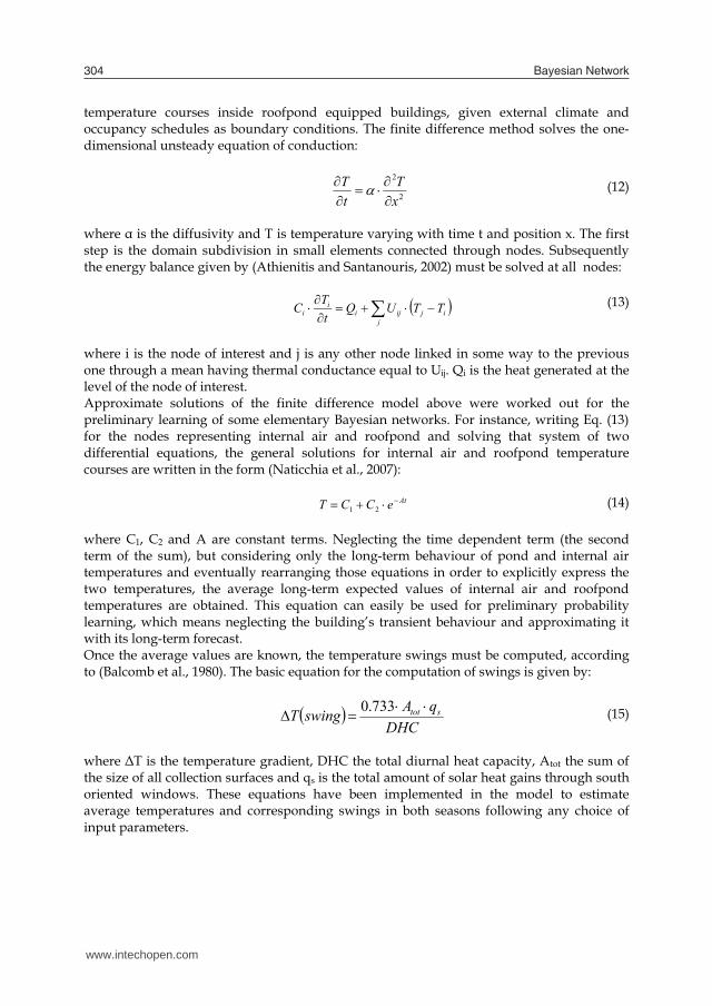
temperature courses inside roofpond equipped buildings, given external climate and occupancy schedules as boundary conditions. The finite difference method solves the one-dimensional unsteady equation of conduction:

2

2

xT

tT

(12)

where α is the diffusivity and T is temperature varying with time t and position x. The first step is the domain subdivision in small elements connected through nodes. Subsequently the energy balance given by (Athienitis and Santanouris, 2002) must be solved at all nodes:

j

ijijii

i TTUQtTC (13)

where i is the node of interest and j is any other node linked in some way to the previous one through a mean having thermal conductance equal to Uij. Qi is the heat generated at the level of the node of interest. Approximate solutions of the finite difference model above were worked out for the preliminary learning of some elementary Bayesian networks. For instance, writing Eq. (13) for the nodes representing internal air and roofpond and solving that system of two differential equations, the general solutions for internal air and roofpond temperature courses are written in the form (Naticchia et al., 2007):

AteCCT 21 (14)

where C1, C2 and A are constant terms. Neglecting the time dependent term (the second term of the sum), but considering only the long-term behaviour of pond and internal air temperatures and eventually rearranging those equations in order to explicitly express the two temperatures, the average long-term expected values of internal air and roofpond temperatures are obtained. This equation can easily be used for preliminary probability learning, which means neglecting the building’s transient behaviour and approximating it with its long-term forecast. Once the average values are known, the temperature swings must be computed, according to (Balcomb et al., 1980). The basic equation for the computation of swings is given by:

DHC

qAswingT stot 733.0 (15)

where ΔT is the temperature gradient, DHC the total diurnal heat capacity, Atot the sum of the size of all collection surfaces and qs is the total amount of solar heat gains through south oriented windows. These equations have been implemented in the model to estimate average temperatures and corresponding swings in both seasons following any choice of input parameters.

4.4 Example of model development The Bayesian model for glazed saddlebacked roofponds was built by combining, through the OOBNs tool, several networks which simulate the thermal behaviour of roofpond equipped buildings with other networks for the estimation of the parameters acting as inputs to the previous ones, leading, finally, to one decision network. The model was based on the platform provided by the program software Hugin ExpertTM. In particular, and referring to Fig. 5, the whole model was organized according to three different levels: - the first level includes seven elementary networks to compute solar heat gains in both seasons, split into attic and main room contributions, besides the needed climatic inputs; - the eight second level networks compute the internal average air temperatures and swings for both the roofpond building and its benchmark, when operating in heating and cooling modes; - the third level is made up of one decision model, solving the problem of choosing the best combination of input variables to optimize the project, finding the best trade-off between benefits pursued in the cold and warm season.

4.4.1 Development of the first level Elementary networks no. 4, 5, 6 and 7 estimate solar gains through the attic and south oriented windows respectively, in the form of mean values in both seasons for the roofpond equipped building and its benchmark. The basic relation implemented is as follows:

SHGCII ext int (16) where I represents irradiation and SHGC is the solar heat gain coefficient (Athienitis and Santanouris, 2002). Networks no. 1, 2 and 3 estimate the input parameters necessary for the computation above, such as average sky temperature and emissivity, irradiation and its angle of incidence on external windows, according to methods suggested by available literature (Balcomb et al, 1980; ASHRAE, 2001), also neglecting non-south oriented window contributions for solar gains. These parameters vary according to climate and building features.

4.4.2 Development of the second level Four elementary networks of level no. 2 were devoted to computing the average internal temperatures in the attic and internal rooms of the roofpond building and its benchmark in both seasons. In particular, networks no. 8 and 9 (the second depicted in Fig. 6) estimate pond and internal temperatures in summer and winter respectively for the roofpond equipped building, based on outputs from the first level networks and other user input parameters. Winter average long-term internal temperatures were computed according to analytical relations put in the form of eq. (14), which has the advantage of being arranged in explicit form. It is a function of heat gains (pond, solar and internal) and losses, mainly due to envelopes and air ventilation (Lord, 1999).

www.intechopen.com


temperature courses inside roofpond equipped buildings, given external climate and occupancy schedules as boundary conditions. The finite difference method solves the one-dimensional unsteady equation of conduction:

2

2

xT

tT

(12)

where α is the diffusivity and T is temperature varying with time t and position x. The first step is the domain subdivision in small elements connected through nodes. Subsequently the energy balance given by (Athienitis and Santanouris, 2002) must be solved at all nodes:

j

ijijii

i TTUQtTC (13)

where i is the node of interest and j is any other node linked in some way to the previous one through a mean having thermal conductance equal to Uij. Qi is the heat generated at the level of the node of interest. Approximate solutions of the finite difference model above were worked out for the preliminary learning of some elementary Bayesian networks. For instance, writing Eq. (13) for the nodes representing internal air and roofpond and solving that system of two differential equations, the general solutions for internal air and roofpond temperature courses are written in the form (Naticchia et al., 2007):

AteCCT 21 (14)

where C1, C2 and A are constant terms. Neglecting the time dependent term (the second term of the sum), but considering only the long-term behaviour of pond and internal air temperatures and eventually rearranging those equations in order to explicitly express the two temperatures, the average long-term expected values of internal air and roofpond temperatures are obtained. This equation can easily be used for preliminary probability learning, which means neglecting the building’s transient behaviour and approximating it with its long-term forecast. Once the average values are known, the temperature swings must be computed, according to (Balcomb et al., 1980). The basic equation for the computation of swings is given by:

DHC

qAswingT stot 733.0 (15)

where ΔT is the temperature gradient, DHC the total diurnal heat capacity, Atot the sum of the size of all collection surfaces and qs is the total amount of solar heat gains through south oriented windows. These equations have been implemented in the model to estimate average temperatures and corresponding swings in both seasons following any choice of input parameters.

4.4 Example of model development The Bayesian model for glazed saddlebacked roofponds was built by combining, through the OOBNs tool, several networks which simulate the thermal behaviour of roofpond equipped buildings with other networks for the estimation of the parameters acting as inputs to the previous ones, leading, finally, to one decision network. The model was based on the platform provided by the program software Hugin ExpertTM. In particular, and referring to Fig. 5, the whole model was organized according to three different levels: - the first level includes seven elementary networks to compute solar heat gains in both seasons, split into attic and main room contributions, besides the needed climatic inputs; - the eight second level networks compute the internal average air temperatures and swings for both the roofpond building and its benchmark, when operating in heating and cooling modes; - the third level is made up of one decision model, solving the problem of choosing the best combination of input variables to optimize the project, finding the best trade-off between benefits pursued in the cold and warm season.

4.4.1 Development of the first level Elementary networks no. 4, 5, 6 and 7 estimate solar gains through the attic and south oriented windows respectively, in the form of mean values in both seasons for the roofpond equipped building and its benchmark. The basic relation implemented is as follows:

SHGCII ext int (16) where I represents irradiation and SHGC is the solar heat gain coefficient (Athienitis and Santanouris, 2002). Networks no. 1, 2 and 3 estimate the input parameters necessary for the computation above, such as average sky temperature and emissivity, irradiation and its angle of incidence on external windows, according to methods suggested by available literature (Balcomb et al, 1980; ASHRAE, 2001), also neglecting non-south oriented window contributions for solar gains. These parameters vary according to climate and building features.

4.4.2 Development of the second level Four elementary networks of level no. 2 were devoted to computing the average internal temperatures in the attic and internal rooms of the roofpond building and its benchmark in both seasons. In particular, networks no. 8 and 9 (the second depicted in Fig. 6) estimate pond and internal temperatures in summer and winter respectively for the roofpond equipped building, based on outputs from the first level networks and other user input parameters. Winter average long-term internal temperatures were computed according to analytical relations put in the form of eq. (14), which has the advantage of being arranged in explicit form. It is a function of heat gains (pond, solar and internal) and losses, mainly due to envelopes and air ventilation (Lord, 1999).

www.intechopen.com

Bayesian Network306

Fig. 5. OOBN representation the whole Bayesian model (a total of 16 networks made up of 219 variable nodes), where only interface nodes are visible. The case of network no. 8 regarding summer behaviour was slightly more complicated, because the application of thermal balance equations to the main room and attic of the roofpond equipped buildings leads to a system with no explicit variables: in this case pond temperature is affected not only by its exchange with the interior but also with the sky. Hence, an explicit equation built on many statistical observations generated by a system including both exchanges between the pond and the interior and between the pond and the exterior. This statistical empirical equation was used to estimate pond temperatures in function of the sky and external conditions. Thermal exchanges with the sky and the interior were inferred from this equation. Validation showed that the model is accurate with an error never exceeding 10%, which was considered as acceptable for preliminary learning. Similar approaches were used to build networks no. 10 and 11, relative to benchmarks, which are simpler given the absence of the roofpond. The other networks are relative to temperature oscillation estimation, in accordance with the theory related to eq. (15) (Balcomb et al., 1980).

4.4.3 Development of the third level Considering that optimizing design choices for winter periods does not guarantee that the same holds for the summer, at this level one large network implementing an objective function to be maximized was set up. It considers two contributions: economic savings deriving from winter benefits that the roofpond determines with respect to its benchmark and from summer benefits. The general form of the objective function is given by:

ch EESEESEES 5.2 (17) where expected energy savings (EES) in the cooling mode (EESc) are more important than those in the heating mode (EESh), because of the difference in fuel and electricity prices. Each term includes energy saving derived from shifting the average temperatures closer to the comfort value and reducing the temperature oscillations around the mean; in addition climate influence and the whole thermal inertia of the building under development are considered. Further details about the model can be found in (Naticchia et al., 2007)

Fig. 6. Elementary network no. 9.

4.5 Model refinement and validation After having implemented the analytical relations into the networks for the approximate relationships in paragraph 4.4, they were subsequently refined using empirical data and by monitoring this process through sensitivity analysis and case-based reasoning, according to the procedure suggested in paragraph 4.1. This paragraph will show some examples of how this could be performed, as it can be applied to any model under development. It has the practical advantage of using all the observations which derive from experiments and simulations worked out by complex software tools. In the particular case of roofponds, the finite difference model described in paragraph 4.3 and based on eq. (13) was implemented on a wide set of real cases to build numerous databases used to implement the sequential updating (paragraph 4.1) on the preliminary conditional probability tables, derived from the equations in paragraph 4.4. This sequential

www.intechopen.com


Fig. 5. OOBN representation the whole Bayesian model (a total of 16 networks made up of 219 variable nodes), where only interface nodes are visible. The case of network no. 8 regarding summer behaviour was slightly more complicated, because the application of thermal balance equations to the main room and attic of the roofpond equipped buildings leads to a system with no explicit variables: in this case pond temperature is affected not only by its exchange with the interior but also with the sky. Hence, an explicit equation built on many statistical observations generated by a system including both exchanges between the pond and the interior and between the pond and the exterior. This statistical empirical equation was used to estimate pond temperatures in function of the sky and external conditions. Thermal exchanges with the sky and the interior were inferred from this equation. Validation showed that the model is accurate with an error never exceeding 10%, which was considered as acceptable for preliminary learning. Similar approaches were used to build networks no. 10 and 11, relative to benchmarks, which are simpler given the absence of the roofpond. The other networks are relative to temperature oscillation estimation, in accordance with the theory related to eq. (15) (Balcomb et al., 1980).

4.4.3 Development of the third level Considering that optimizing design choices for winter periods does not guarantee that the same holds for the summer, at this level one large network implementing an objective function to be maximized was set up. It considers two contributions: economic savings deriving from winter benefits that the roofpond determines with respect to its benchmark and from summer benefits. The general form of the objective function is given by:

ch EESEESEES 5.2 (17) where expected energy savings (EES) in the cooling mode (EESc) are more important than those in the heating mode (EESh), because of the difference in fuel and electricity prices. Each term includes energy saving derived from shifting the average temperatures closer to the comfort value and reducing the temperature oscillations around the mean; in addition climate influence and the whole thermal inertia of the building under development are considered. Further details about the model can be found in (Naticchia et al., 2007)

Fig. 6. Elementary network no. 9.

4.5 Model refinement and validation After having implemented the analytical relations into the networks for the approximate relationships in paragraph 4.4, they were subsequently refined using empirical data and by monitoring this process through sensitivity analysis and case-based reasoning, according to the procedure suggested in paragraph 4.1. This paragraph will show some examples of how this could be performed, as it can be applied to any model under development. It has the practical advantage of using all the observations which derive from experiments and simulations worked out by complex software tools. In the particular case of roofponds, the finite difference model described in paragraph 4.3 and based on eq. (13) was implemented on a wide set of real cases to build numerous databases used to implement the sequential updating (paragraph 4.1) on the preliminary conditional probability tables, derived from the equations in paragraph 4.4. This sequential

www.intechopen.com

Bayesian Network308

updating refines, at each step, the parameters of the Dirichlet distributions underlying the networks, until it optimizes the two quality indices described in paragraph 4.1. Defining as “theoretical experience” the a priori information inserted through simplified analytical laws and “experimental experience” the information deriving from further observations, this method allows the optimum ratio to be found between the importance given to the first and second samples with the aim of learning the Dirichlet parameters. This procedure must be applied to each elementary network included in the model. For instance, let us consider the Bayesian Network no. 6 of level 1 (Fig. 7), relative to the computation of the average hourly SHGC value for the attic window of the roofpond building in winter for direct and diffuse radiation coming from the exterior. After the first learning, based on the use of approximate analytical relationships, a database was generated through accurate simulation. Three values of RTE were then tried: RTE = 10/1; RTE = 3/1; RTE = 1/1. Tab 2 shows LOI values computed in function both of each RTE value chosen and of evidence imposed to parent variables. It can be noticed that RTE = 1/1 gives back the LOI values lower than the initial theoretical model, meaning that entropy is getting closer to zero and that probability distributions are more expressive.

Fig. 7. Graphical structure of elementary network no. 6. In addition, Tab. 3 shows that adding empirical evidence with RTE = 1/1 redirects the values computed by the network towards the real values. In order to perform this case-based reasoning it is necessary to divide any dataset into two parts: the first (and bigger) is generally used for model learning and the second (smaller) is generally used to compare the data provided by the network with the ones recorded by testing or simulation. In this case 90% of the data were used for model learning and 10% for model validation according to case-based reasoning. It was evident that adding further experience to this elementary network did not improve the output of the network, which means that it reached a flat point, beyond which no improvements can be obtained at LOI level. Case-based reasoning must be evaluated on the network’s capability to estimate the correct value for output variables: to that end the interval or contiguous intervals with the highest probability values must be checked. Fig. 8 shows how probability propagation algorithms update output variables probability according to evidence on input variables: black bars are relative to evidence assignment,

while the other probability values are timely and automatically recomputed by the network according to those inputs. Query node Evidence LOI for

theoretical model

LOI for RTE = 1/10

LOI for RTE = 1/3

LOI for RTE = 1/1

Qauh None 2.4 2.4 2.42 2.43

Qauh Ta=“0 to 50”, BIA = 9000 to 12000

1.08 0.63 0.88 0.9

Qauh Ta=“0 to 50”, BIA = 3000 to 6000”

0.99 1.06 1.06 0.87

Table 2. Sensitivity analysis. Query Evidence Results from

theoretical model Results from RTE = 10/1

Results from RTE = 1/1

Real value

Qauh Ta=“0 to 50”, BIA = 3000 to 6000”

70 to 90 (91.6%) 70 to 90 (92.9%)

70 to 90 (97.04%)

83.8

Qauh Ta=“0 to 50”, BIA = 3000 to 6000”

70 to 90 (49.9%) 90 to 110 (49.9%)

70 to 90 (49.9%) 90 to 110 (45.4%)

50 to 70 (25.2%) 70 to 90 (49.09%)

69.4

Table 3. Case-based reasoning for accuracy survey.

Fig. 8. Example of probability updating for elementary network no. 6.

www.intechopen.com


updating refines, at each step, the parameters of the Dirichlet distributions underlying the networks, until it optimizes the two quality indices described in paragraph 4.1. Defining as “theoretical experience” the a priori information inserted through simplified analytical laws and “experimental experience” the information deriving from further observations, this method allows the optimum ratio to be found between the importance given to the first and second samples with the aim of learning the Dirichlet parameters. This procedure must be applied to each elementary network included in the model. For instance, let us consider the Bayesian Network no. 6 of level 1 (Fig. 7), relative to the computation of the average hourly SHGC value for the attic window of the roofpond building in winter for direct and diffuse radiation coming from the exterior. After the first learning, based on the use of approximate analytical relationships, a database was generated through accurate simulation. Three values of RTE were then tried: RTE = 10/1; RTE = 3/1; RTE = 1/1. Tab 2 shows LOI values computed in function both of each RTE value chosen and of evidence imposed to parent variables. It can be noticed that RTE = 1/1 gives back the LOI values lower than the initial theoretical model, meaning that entropy is getting closer to zero and that probability distributions are more expressive.

Fig. 7. Graphical structure of elementary network no. 6. In addition, Tab. 3 shows that adding empirical evidence with RTE = 1/1 redirects the values computed by the network towards the real values. In order to perform this case-based reasoning it is necessary to divide any dataset into two parts: the first (and bigger) is generally used for model learning and the second (smaller) is generally used to compare the data provided by the network with the ones recorded by testing or simulation. In this case 90% of the data were used for model learning and 10% for model validation according to case-based reasoning. It was evident that adding further experience to this elementary network did not improve the output of the network, which means that it reached a flat point, beyond which no improvements can be obtained at LOI level. Case-based reasoning must be evaluated on the network’s capability to estimate the correct value for output variables: to that end the interval or contiguous intervals with the highest probability values must be checked. Fig. 8 shows how probability propagation algorithms update output variables probability according to evidence on input variables: black bars are relative to evidence assignment,

while the other probability values are timely and automatically recomputed by the network according to those inputs. Query node Evidence LOI for

theoretical model

LOI for RTE = 1/10

LOI for RTE = 1/3

LOI for RTE = 1/1

Qauh None 2.4 2.4 2.42 2.43

Qauh Ta=“0 to 50”, BIA = 9000 to 12000

1.08 0.63 0.88 0.9

Qauh Ta=“0 to 50”, BIA = 3000 to 6000”

0.99 1.06 1.06 0.87

Table 2. Sensitivity analysis. Query Evidence Results from

theoretical model Results from RTE = 10/1

Results from RTE = 1/1

Real value

Qauh Ta=“0 to 50”, BIA = 3000 to 6000”

70 to 90 (91.6%) 70 to 90 (92.9%)

70 to 90 (97.04%)

83.8

Qauh Ta=“0 to 50”, BIA = 3000 to 6000”

70 to 90 (49.9%) 90 to 110 (49.9%)

70 to 90 (49.9%) 90 to 110 (45.4%)

50 to 70 (25.2%) 70 to 90 (49.09%)

69.4

Table 3. Case-based reasoning for accuracy survey.

Fig. 8. Example of probability updating for elementary network no. 6.

www.intechopen.com

Bayesian Network310

The same procedure was applied for the other networks of the first and second levels. For instance, network no. 11 is optimized by assigning RTE = 1/1; networks no. 8 and 10 were optimized by assigning RTE = 1/5. In general, this method gives back the amount of experimental data which is sufficient to guarantee good estimations and it can be applied every time technology developers are able to perform controlled tests or software simulations.

5. Applications of the final model

5.1 Overview of the model’s applicability At this level, each sub-network constituting the overall explicit whole network has successfully undergone a validation procedure. Three basic practical applications of Bayesian reasoning within the architectural design profession are (Naticchia et al., 2007):

- determination of the best design solution among several possibilities; - optimal sizing of building parameters; - approximate sizing under conditions of uncertainty.

In the first case, designers could be supported in the process of discerning the best choice among several likely building configurations using the model’s energy efficiency-based objective function. The second aspect is typical of a rough-sizing process: often, before a designer may size any building parameter, the viable choices on the market need to be investigated in terms of various issues. This probabilistic model allows bottom-up reasoning, that is to say, querying the objective function in order to derive the proper values that yield the highest utility for the particular issue being considered. Finally, when there is no certain knowledge about some given parameters (e.g. type of glazing for south facing windows), the designer should be able to make inferences in the case of uncertain distribution over several values and give back a probability distribution for the objective function that is useful for carrying out an exploration of the two previously mentioned design aspects.

5.2 First application case: choice of the best design solution Suppose a designer specifies a glazed, saddleback roofpond application for a one-storey 100 m2 residence located in Salt Lake City, Utah. All the architectural features have been determined except for the total area of the solar attic window. Two available options consist in an area equal to either 50% or 35% of the total floor. All the input values were inserted into the model: climatic parameters in accordance with Salt Lake City characteristics; “5a double clear” type of glass; south facing window area equal to 5 m2; total area of the other windows equal to 35 m2. Thermal transmittance of walls and attic respectively equal to 0.035 W/(m2·K) and 0.02 W/(m2·K); “5/8 in gypsum panel” installed as a ceiling; “4 in thick brick” used for walls; 0.3 m deep pond. Fig. 9 depicts some of the results obtained from the two assumed cases. It can be noticed from temperature diagrams that in the second case (attic window area equal to 35% of the floor) the temperature difference between the roofpond building and the benchmark working in heating mode is higher than in the second, meaning that it brings higher positive benefits in winter. On the contrary, the second case is less advantageous in the summer. Similar remarks could be confirmed for temperature swings. Given this ambiguous situation, the use of the objective function (in BN

no. 16) with the computation of the expected utility, makes us conclude that the second option is better. This is likely to be due to the lower winter losses caused by the smaller area of glazing. a) case no. 1

Sub-network pond heating Sub-net. benchmark heating Objective Function

Sub-network pond cooling Sub-net. benchmark heating Expected utility

Case no. 1: EU = 115.1

b) case no. 2 Sub-network pond heating Sub-net. benchmark heating Objective Function


Case no. 2: EU = 127.4

Fig. 9. Example of selection of the best design option between two possibilities.

5.3 Second application case: optimal sizing of building parameters As a second scenario let us assume that a designer is employing a roofpond strategy in a passively conditioned building made up of a detached single-family dwelling of 200 m2 in Seattle, Washington. The designer is free to determine the area of south-facing glazing. Some input parameters include: thermal transmittance of walls equal to 0.04 W/(m2·K), while for the attic equal to 0.02 W/(m2·K); area of non-south facing windows equal to 20 m2; the glazed window attic area being 0.35 times the floor area; ceiling of “1/2 in gypsum panel” type, wall of “4 in thick hollow brick fired clay” type and 0.3 m deep pond on the roof. The first case in Fig. 10 depicts the results obtained at the level of the Objective Function and the south facing window area, that was left free to vary. The probability

www.intechopen.com


The same procedure was applied for the other networks of the first and second levels. For instance, network no. 11 is optimized by assigning RTE = 1/1; networks no. 8 and 10 were optimized by assigning RTE = 1/5. In general, this method gives back the amount of experimental data which is sufficient to guarantee good estimations and it can be applied every time technology developers are able to perform controlled tests or software simulations.

5. Applications of the final model

5.1 Overview of the model’s applicability At this level, each sub-network constituting the overall explicit whole network has successfully undergone a validation procedure. Three basic practical applications of Bayesian reasoning within the architectural design profession are (Naticchia et al., 2007):

- determination of the best design solution among several possibilities; - optimal sizing of building parameters; - approximate sizing under conditions of uncertainty.

In the first case, designers could be supported in the process of discerning the best choice among several likely building configurations using the model’s energy efficiency-based objective function. The second aspect is typical of a rough-sizing process: often, before a designer may size any building parameter, the viable choices on the market need to be investigated in terms of various issues. This probabilistic model allows bottom-up reasoning, that is to say, querying the objective function in order to derive the proper values that yield the highest utility for the particular issue being considered. Finally, when there is no certain knowledge about some given parameters (e.g. type of glazing for south facing windows), the designer should be able to make inferences in the case of uncertain distribution over several values and give back a probability distribution for the objective function that is useful for carrying out an exploration of the two previously mentioned design aspects.

5.2 First application case: choice of the best design solution Suppose a designer specifies a glazed, saddleback roofpond application for a one-storey 100 m2 residence located in Salt Lake City, Utah. All the architectural features have been determined except for the total area of the solar attic window. Two available options consist in an area equal to either 50% or 35% of the total floor. All the input values were inserted into the model: climatic parameters in accordance with Salt Lake City characteristics; “5a double clear” type of glass; south facing window area equal to 5 m2; total area of the other windows equal to 35 m2. Thermal transmittance of walls and attic respectively equal to 0.035 W/(m2·K) and 0.02 W/(m2·K); “5/8 in gypsum panel” installed as a ceiling; “4 in thick brick” used for walls; 0.3 m deep pond. Fig. 9 depicts some of the results obtained from the two assumed cases. It can be noticed from temperature diagrams that in the second case (attic window area equal to 35% of the floor) the temperature difference between the roofpond building and the benchmark working in heating mode is higher than in the second, meaning that it brings higher positive benefits in winter. On the contrary, the second case is less advantageous in the summer. Similar remarks could be confirmed for temperature swings. Given this ambiguous situation, the use of the objective function (in BN

no. 16) with the computation of the expected utility, makes us conclude that the second option is better. This is likely to be due to the lower winter losses caused by the smaller area of glazing. a) case no. 1

Sub-network pond heating Sub-net. benchmark heating Objective Function


Case no. 1: EU = 115.1

b) case no. 2 Sub-network pond heating Sub-net. benchmark heating Objective Function


Case no. 2: EU = 127.4

Fig. 9. Example of selection of the best design option between two possibilities.

5.3 Second application case: optimal sizing of building parameters As a second scenario let us assume that a designer is employing a roofpond strategy in a passively conditioned building made up of a detached single-family dwelling of 200 m2 in Seattle, Washington. The designer is free to determine the area of south-facing glazing. Some input parameters include: thermal transmittance of walls equal to 0.04 W/(m2·K), while for the attic equal to 0.02 W/(m2·K); area of non-south facing windows equal to 20 m2; the glazed window attic area being 0.35 times the floor area; ceiling of “1/2 in gypsum panel” type, wall of “4 in thick hollow brick fired clay” type and 0.3 m deep pond on the roof. The first case in Fig. 10 depicts the results obtained at the level of the Objective Function and the south facing window area, that was left free to vary. The probability

www.intechopen.com

Bayesian Network312

distribution relative to the area of south windows considers the first interval as the only one not to be chosen, while the others cannot be excluded at this level. If the objective function value is maximized by the introduction of evidence in its highest interval, the south facing probability distribution changes accordingly: it prompts an optimum value between two intervals having approximately the same probability, that can be interpreted as being on average 7 m2. Moreover, in order to show how this model is sensitive to the choice of the decision variable, the possibility that the total area of non-south facing glazing is changed from 20 to 35 m2 is considered, leaving all the other parameters unchanged (case no. 2 in Fig. 10). The probabilistic model has the ability to adjust itself: the objective function value now suggests that it would be more opportune to increase the south facing glazing to between 7 and 12 m2. Case no. 1 Objective function (O.F.)

South windows Maximized O. F. Final south windows

Case no. 2 Objective function (O.F.)


Fig. 10. Example of optimization of a building parameter.

5.4 Third application case: approximate sizing under conditions of uncertainty In the third scenario a designer for a one-storey residence in Seattle, Washington is implementing the glazed saddleback roofpond application and needs to determine the most appropriate type of glazing for all the building windows, while the one relative to skylights of the solar collection space above the roofpond was chosen to be “5a double clear”. For the other windows the designer must choose between “5a double clear” and “17c double low-emission” glazing. In addition to this choice, there is uncertainty regarding the optimum area of the south facing glazing, which will be determined after the preliminary design in accordance with other needs. At this juncture, it will suffice to approximate that there is a 30% probability of choosing a total area of 5.5 m2 and a 70% chance of choosing a total area of 9.5 m2. Fig. 11 depicts the likelihood distribution inserted as the variable “area of south windows”, which lets the network reason under uncertainty.

Fig. 11. Likelihood distribution inserted in the network Other decision variables are: floor area of 200 m2; area of non-south facing windows of 20 m2; ratio of glazed attic surface out of floor equal to 0.35. Sub-network pond heating Sub-net. benchmark heating Objective Function


Case no. 1: EU = 257.8

Fig. 12. Expected utility estimation under conditions of uncertainty for the 1st option In the case of Fig. 12 all the windows are assigned as the “5a double clear” type. The consequent result is an expected utility of 257.8. In the second case (implemented in a way similar to the first case) all the building windows were assigned a “17c low emission” glass type, which gave back an expected utility of 293.25. The results suggest that the “17c double low emission” glazing would work better in terms of thermal performance. This is probably due to the thermal transmittance of the glazed windows utilized in the second case, which is lower than that found in the first case (2.89 versus 3.25 W/(m2·K)).

6. Conclusion

Bayesian Networks are a powerful tool to build accurate models for supporting professional architects in the preliminary design phase of buildings. Their friendly graphical structure is easy to interpret and their learning algorithms are capable of reproducing even non-linear relationships relative to complex phenomena, which involve a number of different sub-processes. This chapter deals with a procedure that research scientists can adopt to develop Bayesian networks for modelling the behaviour of new technologies and favouring their fast spread into the market, simplifying the task of designers who have to make design choices based on estimated building parameters. Developing such models involves discerning which kind of knowledge and data must be inserted in order to obtain a reliable network. For that purpose, this study suggests breaking down the whole process into sub-processes, each simulated by one elementary network, according to the OOBNs approach. Causal

www.intechopen.com


distribution relative to the area of south windows considers the first interval as the only one not to be chosen, while the others cannot be excluded at this level. If the objective function value is maximized by the introduction of evidence in its highest interval, the south facing probability distribution changes accordingly: it prompts an optimum value between two intervals having approximately the same probability, that can be interpreted as being on average 7 m2. Moreover, in order to show how this model is sensitive to the choice of the decision variable, the possibility that the total area of non-south facing glazing is changed from 20 to 35 m2 is considered, leaving all the other parameters unchanged (case no. 2 in Fig. 10). The probabilistic model has the ability to adjust itself: the objective function value now suggests that it would be more opportune to increase the south facing glazing to between 7 and 12 m2. Case no. 1 Objective function (O.F.)


Case no. 2 Objective function (O.F.)


Fig. 10. Example of optimization of a building parameter.

5.4 Third application case: approximate sizing under conditions of uncertainty In the third scenario a designer for a one-storey residence in Seattle, Washington is implementing the glazed saddleback roofpond application and needs to determine the most appropriate type of glazing for all the building windows, while the one relative to skylights of the solar collection space above the roofpond was chosen to be “5a double clear”. For the other windows the designer must choose between “5a double clear” and “17c double low-emission” glazing. In addition to this choice, there is uncertainty regarding the optimum area of the south facing glazing, which will be determined after the preliminary design in accordance with other needs. At this juncture, it will suffice to approximate that there is a 30% probability of choosing a total area of 5.5 m2 and a 70% chance of choosing a total area of 9.5 m2. Fig. 11 depicts the likelihood distribution inserted as the variable “area of south windows”, which lets the network reason under uncertainty.

Fig. 11. Likelihood distribution inserted in the network Other decision variables are: floor area of 200 m2; area of non-south facing windows of 20 m2; ratio of glazed attic surface out of floor equal to 0.35. Sub-network pond heating Sub-net. benchmark heating Objective Function


Case no. 1: EU = 257.8

Fig. 12. Expected utility estimation under conditions of uncertainty for the 1st option In the case of Fig. 12 all the windows are assigned as the “5a double clear” type. The consequent result is an expected utility of 257.8. In the second case (implemented in a way similar to the first case) all the building windows were assigned a “17c low emission” glass type, which gave back an expected utility of 293.25. The results suggest that the “17c double low emission” glazing would work better in terms of thermal performance. This is probably due to the thermal transmittance of the glazed windows utilized in the second case, which is lower than that found in the first case (2.89 versus 3.25 W/(m2·K)).

6. Conclusion

Bayesian Networks are a powerful tool to build accurate models for supporting professional architects in the preliminary design phase of buildings. Their friendly graphical structure is easy to interpret and their learning algorithms are capable of reproducing even non-linear relationships relative to complex phenomena, which involve a number of different sub-processes. This chapter deals with a procedure that research scientists can adopt to develop Bayesian networks for modelling the behaviour of new technologies and favouring their fast spread into the market, simplifying the task of designers who have to make design choices based on estimated building parameters. Developing such models involves discerning which kind of knowledge and data must be inserted in order to obtain a reliable network. For that purpose, this study suggests breaking down the whole process into sub-processes, each simulated by one elementary network, according to the OOBNs approach. Causal

www.intechopen.com

Bayesian Network314

relationships among variables in every elementary network are then learnt, starting from both simplified analytical relationships and from experimental data or those deriving from numerical simulations: the procedure proposed in this chapter suggests how to measure the level of quality of the network, which can gradually be tuned by changing the importance of subjective relationships, with respect to the data. Once the model is built, it has the benefit of performing both predictive and diagnostic reasoning, as well as reasoning under conditions of uncertainty. Therefore it is capable of supporting architects in several single or combined basic tasks: the determination of the best design solution among different available choices; the optimal sizing of building parameters; the approximate sizing under conditions of uncertainty. These applications include what could realistically be of interest for professional designers, who would use the Bayesian models as an expert system to drive them towards fast and accurate designing.

7. References

Alefeld, G. and Herzberg, J. (1983) Introduction to interval computation, Academic Press, New York, NY.

Athienitis A.K., Santanouris M., (2002) Thermal Analysis and Design of Passive Solar Buildings, James and James Science Publisher, London, 2002

Balcomb J.D., Barley D., McFarland R., Perry J., Wray W., Noll S., Passive Solar Design Handbook, vol. 2, Passive Solar Design Analysis, US Department of Energy, Washington, DC, 1980.

Boborow, D. G., (1984) Qualitative reasoning about physical systems, MIT Press, Cambridge, UK.

Charniak, E., Bayesian networks without tears, Artificial Intelligence magazine, vol. 12, no. 4, pp. 50-63, 1991.

Evans, M., Hastings, N., Peacock, B., (1993) Statistical distributions, 2nd edition, John Wiley and sons, New York.

Fernández-González, A. Characterizing Thermal Comfort in Five Different Passive Solar Heating Strategies. Proceedings of the Architectural Research Centers Consortium 2003 Conference, April 10-12, Tempe, AZ.

Fernandez-Gonzalez A., RP_performance: a design tool to simulate the thermal performance of skytherm North roofpond systems, in: Proceedings of the 33rd American Solar Energy Society National Conference, Portland, OR, July 9–14, 2004.

Heckerman, D. (1996) Bayesian Networks for knowledge discovery, in Fayyad, U.M., Piatetsky-Shapiro, G., Smyth, P., Uthurusamy, R., Advances in knowledge discovery and data mining, AAAI Press/MIT Press.

Hugin Expert, (2008) Hugin API – Reference Manual, version 7.0, Hugin Expert A/S. Jensen, F. V., (2000) Bayesian Networks and decision graphs, Springer-Verlag, New York. Koller, D., and Pfeffer, A., Object-oriented Bayesian networks, in 13th Conference on

Uncertainty in Artificial Intelligence (Morgan Kaufmann, San Francisco, 1997), D. Geiger and P. Shenoy, Eds., pp. 302-313.

Korb, K. B., Nicholson, A. E., (2004) Bayesian artificial intelligence, Chapman & Hall/CRC edition.

Lauría, Eitel J.M.; Duchessi, Peter J.; A methodology for developing Bayesian networks: An application to information technology(IT)implementation, European Journal of Operational Research, v 179, n 1, p 234-252, May 16, 2007.

Lauritzen, S. L., The EM algorithm for graphical association models with missing data, Computational Statistics & Data Analysis, vol.19, pp.191-201, (1995).

Lord D., An interactive,Web-based computer program for thermal design of roofponds, Ph.D. Thesis, California Polytechnic State University, College of Architecture and Environmental Design, Architecture Department, 1999.

Lucas, P.J.F., Bayesian network modeling with qualitative pattern, Artificial Intelligence, vol. 163, pp. 233-263, (2005).

Marlatt, W. P., Murray, K. A., Squier, S. E., (1984) Roofpond systems, Energy Technology Engineering center for the U. S. Department of Energy (contract DE-AM03-76SF00700 ), Canoga Park, California.

Nadkarni, S., Shenoy, P. P., A causal mapping approach to constructing Bayesian networks, Decision support systems, vol. 38, pp. 259-281.

Naticchia, B., De Grassi, M., (2001) Modelling environmental complexity for sustainable design practice (Ch, 9 pp. 135-160), in Towards Sustainable Buildings, N. Maiellaro, Kluwer Academic Publisher, pp. 135-160, Netherlands.

Naticchia B., Fernandez-Gonzalez A., Carbonari A., “Bayesian Network model for the design of roofpond equipped buildings”, Energy and Buildings, vol. 39, 2007, pp. 258-272.

Stein, B., Reynolds, J. S., (2000) Mechanical and electrical equipments for buildings, John Wiley and sons, New York, 9th ed.

Pearl, J., (1988) Probabilistic reasoning in Intelligent Systems: networks of plausible inference, Morgan Kauffman ed., San Mateo, California.

Sadoddin, A., Letcher, R.A., Jakeman, A.J., Newham, L.T.H., A Bayesian decision network approach for assessing the ecological impacts of salinity management, Mathematics and computers in simulation, vol. 69, pp. 162-176.

Spiegelalther, D., Laurintzen, S. L., Sequential updating of conditional probabilities on directed graphical structures, Networks, vol. 20, pp. 579-605.

Van Truong, Luu; Soo-Yong, Kim; Nguyen Van, Tuan; Stephen O., Ogunlana “Quantifying schedule risk in construction projects using Bayesian belief networks”, International Journal of Project Management, v 27, n 1, p 39-50, January 2009.

Weidl, G., Madsen, A.L., Israelson, S., Applications of object-oriented Bayesian networks for condition monitoring, root cause analysis and decision support on operation of complex continuous processes, Computers and Chemical Engineering, vol. 29, pp. 1996-2009.

Wenhui, Liao; Qiang, Ji; Learning Bayesian network parameters under incomplete data with domain knowledge, Pattern Recognition, v 42, n 11, p 3046-3056, November 2009.

Wonnacott, T. H. and Wonnacott, R. J., (1990) Introductory statistics – 5th ed., John Wiley and sons, New York, pp. 582-615.

Zhang, H., Jarzabek, S., A Bayesian Network approach to rational architectural design, ,International Journal of Software Engineering and Knowledge Engineering, v 15, n 4, August, 2005, p 695-717.

www.intechopen.com


relationships among variables in every elementary network are then learnt, starting from both simplified analytical relationships and from experimental data or those deriving from numerical simulations: the procedure proposed in this chapter suggests how to measure the level of quality of the network, which can gradually be tuned by changing the importance of subjective relationships, with respect to the data. Once the model is built, it has the benefit of performing both predictive and diagnostic reasoning, as well as reasoning under conditions of uncertainty. Therefore it is capable of supporting architects in several single or combined basic tasks: the determination of the best design solution among different available choices; the optimal sizing of building parameters; the approximate sizing under conditions of uncertainty. These applications include what could realistically be of interest for professional designers, who would use the Bayesian models as an expert system to drive them towards fast and accurate designing.

7. References

Alefeld, G. and Herzberg, J. (1983) Introduction to interval computation, Academic Press, New York, NY.

Athienitis A.K., Santanouris M., (2002) Thermal Analysis and Design of Passive Solar Buildings, James and James Science Publisher, London, 2002

Balcomb J.D., Barley D., McFarland R., Perry J., Wray W., Noll S., Passive Solar Design Handbook, vol. 2, Passive Solar Design Analysis, US Department of Energy, Washington, DC, 1980.

Boborow, D. G., (1984) Qualitative reasoning about physical systems, MIT Press, Cambridge, UK.

Charniak, E., Bayesian networks without tears, Artificial Intelligence magazine, vol. 12, no. 4, pp. 50-63, 1991.

Evans, M., Hastings, N., Peacock, B., (1993) Statistical distributions, 2nd edition, John Wiley and sons, New York.

Fernández-González, A. Characterizing Thermal Comfort in Five Different Passive Solar Heating Strategies. Proceedings of the Architectural Research Centers Consortium 2003 Conference, April 10-12, Tempe, AZ.

Fernandez-Gonzalez A., RP_performance: a design tool to simulate the thermal performance of skytherm North roofpond systems, in: Proceedings of the 33rd American Solar Energy Society National Conference, Portland, OR, July 9–14, 2004.

Heckerman, D. (1996) Bayesian Networks for knowledge discovery, in Fayyad, U.M., Piatetsky-Shapiro, G., Smyth, P., Uthurusamy, R., Advances in knowledge discovery and data mining, AAAI Press/MIT Press.

Hugin Expert, (2008) Hugin API – Reference Manual, version 7.0, Hugin Expert A/S. Jensen, F. V., (2000) Bayesian Networks and decision graphs, Springer-Verlag, New York. Koller, D., and Pfeffer, A., Object-oriented Bayesian networks, in 13th Conference on

Uncertainty in Artificial Intelligence (Morgan Kaufmann, San Francisco, 1997), D. Geiger and P. Shenoy, Eds., pp. 302-313.

Korb, K. B., Nicholson, A. E., (2004) Bayesian artificial intelligence, Chapman & Hall/CRC edition.

Lauría, Eitel J.M.; Duchessi, Peter J.; A methodology for developing Bayesian networks: An application to information technology(IT)implementation, European Journal of Operational Research, v 179, n 1, p 234-252, May 16, 2007.

Lauritzen, S. L., The EM algorithm for graphical association models with missing data, Computational Statistics & Data Analysis, vol.19, pp.191-201, (1995).

Lord D., An interactive,Web-based computer program for thermal design of roofponds, Ph.D. Thesis, California Polytechnic State University, College of Architecture and Environmental Design, Architecture Department, 1999.

Lucas, P.J.F., Bayesian network modeling with qualitative pattern, Artificial Intelligence, vol. 163, pp. 233-263, (2005).

Marlatt, W. P., Murray, K. A., Squier, S. E., (1984) Roofpond systems, Energy Technology Engineering center for the U. S. Department of Energy (contract DE-AM03-76SF00700 ), Canoga Park, California.

Nadkarni, S., Shenoy, P. P., A causal mapping approach to constructing Bayesian networks, Decision support systems, vol. 38, pp. 259-281.

Naticchia, B., De Grassi, M., (2001) Modelling environmental complexity for sustainable design practice (Ch, 9 pp. 135-160), in Towards Sustainable Buildings, N. Maiellaro, Kluwer Academic Publisher, pp. 135-160, Netherlands.

Naticchia B., Fernandez-Gonzalez A., Carbonari A., “Bayesian Network model for the design of roofpond equipped buildings”, Energy and Buildings, vol. 39, 2007, pp. 258-272.

Stein, B., Reynolds, J. S., (2000) Mechanical and electrical equipments for buildings, John Wiley and sons, New York, 9th ed.

Pearl, J., (1988) Probabilistic reasoning in Intelligent Systems: networks of plausible inference, Morgan Kauffman ed., San Mateo, California.

Sadoddin, A., Letcher, R.A., Jakeman, A.J., Newham, L.T.H., A Bayesian decision network approach for assessing the ecological impacts of salinity management, Mathematics and computers in simulation, vol. 69, pp. 162-176.

Spiegelalther, D., Laurintzen, S. L., Sequential updating of conditional probabilities on directed graphical structures, Networks, vol. 20, pp. 579-605.

Van Truong, Luu; Soo-Yong, Kim; Nguyen Van, Tuan; Stephen O., Ogunlana “Quantifying schedule risk in construction projects using Bayesian belief networks”, International Journal of Project Management, v 27, n 1, p 39-50, January 2009.

Weidl, G., Madsen, A.L., Israelson, S., Applications of object-oriented Bayesian networks for condition monitoring, root cause analysis and decision support on operation of complex continuous processes, Computers and Chemical Engineering, vol. 29, pp. 1996-2009.

Wenhui, Liao; Qiang, Ji; Learning Bayesian network parameters under incomplete data with domain knowledge, Pattern Recognition, v 42, n 11, p 3046-3056, November 2009.

Wonnacott, T. H. and Wonnacott, R. J., (1990) Introductory statistics – 5th ed., John Wiley and sons, New York, pp. 582-615.

Zhang, H., Jarzabek, S., A Bayesian Network approach to rational architectural design, ,International Journal of Software Engineering and Knowledge Engineering, v 15, n 4, August, 2005, p 695-717.

www.intechopen.com

Bayesian Network316

Zhiqiang, Cai; Shudong, Sun; Shubin, Si; Bernard, Yannou; Maintenance management system based on Bayesian networks, 2008 International Seminar on Business and Information Management, ISBIM 2008, v 2, p 42-45, 2009.

Zhu, J.Y., Deshmukh, A., Application of Bayesian decision networks to life cycle engineering in Green design and manufacturing, Engineering applications of Artificial Intelligence, vol. 16, pp. 91-103.

www.intechopen.com

Bayesian NetworkEdited by Ahmed Rebai

ISBN 978-953-307-124-4Hard cover, 432 pagesPublisher SciyoPublished online 18, August, 2010Published in print edition August, 2010

InTech EuropeUniversity Campus STeP Ri Slavka Krautzeka 83/A 51000 Rijeka, Croatia Phone: +385 (51) 770 447 Fax: +385 (51) 686 166www.intechopen.com

InTech ChinaUnit 405, Office Block, Hotel Equatorial Shanghai No.65, Yan An Road (West), Shanghai, 200040, China

Phone: +86-21-62489820 Fax: +86-21-62489821

Bayesian networks are a very general and powerful tool that can be used for a large number of problemsinvolving uncertainty: reasoning, learning, planning and perception. They provide a language that supportsefficient algorithms for the automatic construction of expert systems in several different contexts. The range ofapplications of Bayesian networks currently extends over almost all fields including engineering, biology andmedicine, information and communication technologies and finance. This book is a collection of originalcontributions to the methodology and applications of Bayesian networks. It contains recent developments inthe field and illustrates, on a sample of applications, the power of Bayesian networks in dealing the modeling ofcomplex systems. Readers that are not familiar with this tool, but have some technical background, will find inthis book all necessary theoretical and practical information on how to use and implement Bayesian networksin their own work. There is no doubt that this book constitutes a valuable resource for engineers, researchers,students and all those who are interested in discovering and experiencing the potential of this major tool of thecentury.

How to referenceIn order to correctly reference this scholarly work, feel free to copy and paste the following:

Berardo Naticchia and Alessandro Carbonari (2010). Causal Modelling Based on Bayesian Networks forPreliminary Design of Buildings, Bayesian Network, Ahmed Rebai (Ed.), ISBN: 978-953-307-124-4, InTech,Available from: http://www.intechopen.com/books/bayesian-network/causal-modelling-based-on-bayesian-networks-for-preliminary-design-of-buildings

Causal modelling based on bayesian networks for ...cdn.intechweb.org/pdfs/11956.pdf · Causal...

Documents

Transcript of Causal modelling based on bayesian networks for ...cdn.intechweb.org/pdfs/11956.pdf · Causal...