Causal Inference in Economics and Marketing*

Erhan ŞanlıData Science, Istanbul Sehir Universityerhansanli@std.sehir.edu.tr

Data Science & AI WorkshopAugust 4th, 2018

Istanbul Sehir University

* Hal Varian, 7310-7315 | PNAS | July 5, 2016 | vol. 113 | no. 27

Outline

1. Introduction2. A Motivating Problem3. Fundamental Identity of Causal Inference4. Methods for Estimating Causal Effects5. Conclusion6. References

1. Introduction

Causality: The relationship between an event (the cause) and a second event (the effect), where the second event is understood as a consequence of the first.

Causation can be extremely hard to prove. But data scientists use it very recklessly.

1. Introduction

• Article from The Economist: Ice Cream and IQ. Written by “The Data Team”, the article suggests that “… more ice cream eating might be the solution to poor student score.” Seriously!

Correlation does not imply causation!

• What could cause this?…There may be many explanations..

Look for causation!

1. Introduction

2. A Motivating Problem

• 𝑦 = 𝑆𝑎𝑙𝑒𝑠 𝑖𝑛 𝑐𝑖𝑡𝑦 𝑐• 𝑥 = 𝐴𝑑 𝑠𝑝𝑒𝑛𝑑 𝑖𝑛 𝑐𝑖𝑡𝑦 𝑐• Linear model: 𝑦 = 𝑏 𝑥 + 𝑒 (Center data to eliminate the constant)• 𝑒 = 𝑒𝑟𝑟𝑜𝑟 𝑖𝑛 𝑐𝑖𝑡𝑦 𝑐 (cumulative effect of omitted predictors)

GOAL: Estimate causal effect of changing 𝑥 .

e.g., What would happen if we increased ad spend by 10% in every city?

2. A Motivating Problem-Standard Approach

• Run a least-squares regression of 𝑦 on 𝑥 .• To get a good estimate of b;

• 𝑏 = , ( , ) .

• 𝑏 = ,, = 𝑏 + ,

( , )• Need 𝑐𝑜𝑣 𝑥, 𝑒 = 0.

• This is unlikely when x is chosen by decision makers.• They will choose x based on factors they observe but the analyst does not!

So, the best client for the data analyst is someone who is incompetent and makes choices randomly!

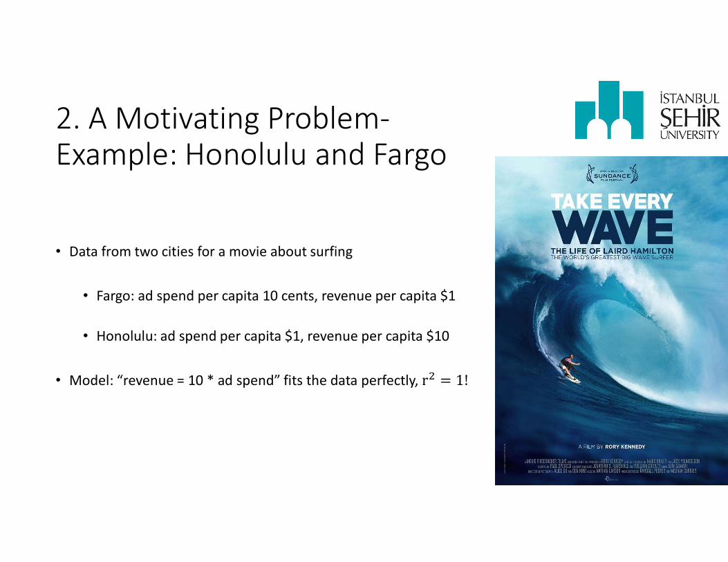
2. A Motivating Problem-Example: Honolulu and Fargo

• Data from two cities for a movie about surfing

• Fargo: ad spend per capita 10 cents, revenue per capita $1

• Honolulu: ad spend per capita $1, revenue per capita $10

• Model: “revenue = 10 * ad spend” fits the data perfectly, r = 1!

2. A Motivating Problem-Example: Honolulu and Fargo

• Honolulu, Hawaii • Fargo, Dakota

2. A Motivating Problem-Example: Honolulu and Fargo

• Honolulu, Hawaii • Fargo, Dakota

Does increasing ad spend in Fargo to $1 result in $10 revenue?For a surfing movie?

What is wrong with the model?

2. What’s wrong?

• Confounding variables are relevant omitted variables (they help predict y) that are also correlated with other predictors.

• They are very common in models involving human choice since decision makers observe important factors that data analyst does not.

CONFOUNDING VARIABLE

(INTEREST IN SURFING)

INDEPENDENT VARIABLE

(X= AD SPEND CHOICES)

DEPENDENT VARIABLE

(Y=REVENUE)

Spurious correlation

2. A Motivating Problem-More examples from economics

• How does fertilizer affect crop yields?• Farmers choose fertilizer application based on land quality(Land quality also affects yield(output): confounding variable)

• How does education affect income?• Students having rich parents or high ability acquire both more education and more income.(Having rich parents affects the predictor and the outcome: confounding variable)

• How does health care affect income?• Those having good jobs tend to have health care.(Having good job is a confounding variable)

2. A Motivating Problem-More examples from economics

Pure observational data is not going to work!

Ideal thing to do is to run an experiment.

But experiments are expensive and sometimes infeasible.

So, what can you learn from observational data when there is no experimentation?

3. Fundamental Identity of Causal Inference• We can decompose the observed outcome of a treatment into two effects:• Outcome for treated – Outcome for untreated

= [Outcome for treated – Outcome for treated if not treated] + [Outcome for treated if not treated – Outcome for untreated]

= Impact of treatment on treated + Selection bias

• The critical concept for understanding causality is the comparison of the actual outcome (what happens to the treated) with the counterfactual (what would have happened if they had not been treated).

• We cannot observe counterfactual, therefore we have to estimate that counterfactual some other way. Machine Learning comes into play!

4. Methods to estimate causal effects from observational data

1. Randomized experiments2. Natural experiments3. Instrumental variables4. Regression discontinuity5. Difference in differences

4. Methods: Randomized experiments• Want to treat subjects at (randomly chosen) times, compare to nontreated times e.g., advertisement. Estimate impact of ad treatment on the advertiser.

• For marketing experiments, use pre-experiment behavior to build a predictive model for outcomes. Use this model to estimate the counterfactual: what would have happened without the treatment

• Train, test, treat, compare (TTTC)• Train: a model on some of your data• Test: a model on holdout data• Treat: apply treatment to treatment group• Compare: outcome for treated to the counterfactual prediction obtained from ML model

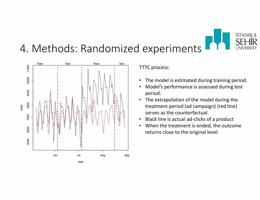
4. Methods: Randomized experimentsTTTC process:

• The model is estimated during training period.• Model’s performance is assessed during test

period.• The extrapolation of the model during the

treatment period (ad campaign) (red line) serves as the counterfactual.

• Black line is actual ad-clicks of a product• When the treatment is ended, the outcome

returns close to the original level.

4. Methods: Natural experimentsExample-Super Bowl and ad impact

Compare sales in treated

cities (home team) to sales in untreated

cities.

Two randomly chosen cities will have 10-15% more ad impressions

Ads are sold months before

it is known which teams

will be playing

Home cities have 10-15 %

larger audience

4. Methods: Instrumental Variables

• A variable that affects the outcome,𝑦 , only via its effect on input,𝑥 , is called an “instrumental variable”.

INSTRUMENTAL VARIABLE

(WINNING THE PLAYOFFS)

X=AD VIEWERSHIP IN

TWO RANDOMLY

CHOSEN CITIES

Y=SALES IN TREATED CITIES

4. Methods: Instrumental VariablesExample• Suppose we want to estimate how air travel responds to change in ticket price (demand)

• Price is chosen by airlines• When times are good, airlines choose high prices and people travel a lot• When times are bad, airlines choose low prices and people don’t travel much• We then find high prices predict high demand, and low prices predict low demand-contrary to

what economics science says-

• Problem is “times are good” is a confounding variable. It affects both price and demand.

• What to do?• Find a good proxy for “times are good” (e.g. GDP), put that into the regression and/or• Find an instrument that moves price but does not directly affect travel; such as a tax, fuel cost,

unionization etc.

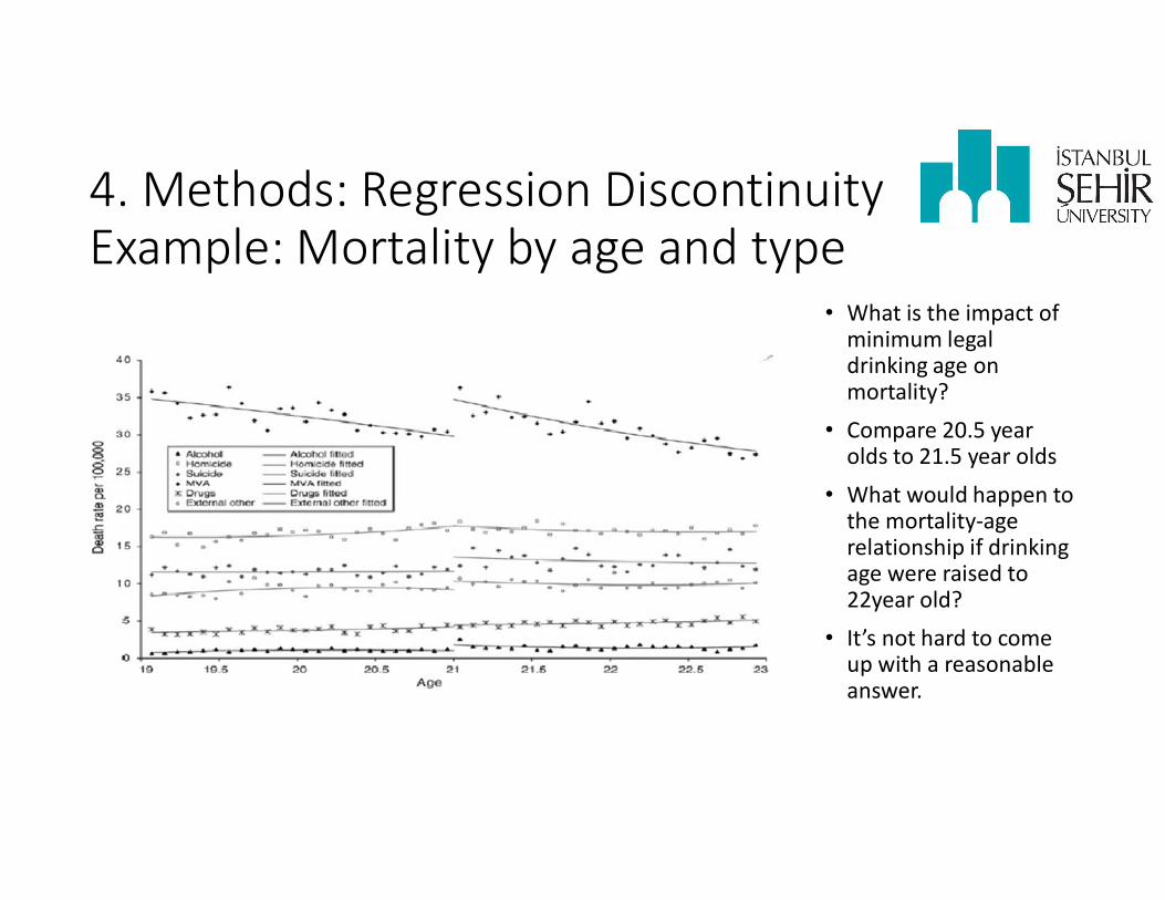
4. Methods: Regression DiscontinuityExample: Mortality by age and type

• What is the impact of minimum legal drinking age on mortality?

• Compare 20.5 year olds to 21.5 year olds

• What would happen to the mortality-age relationship if drinking age were raised to 22year old?

• It’s not hard to come up with a reasonable answer.

4. Methods: Difference in differences• 𝑆 = 𝑠𝑎𝑙𝑒𝑠 𝑎𝑓𝑡𝑒𝑟 𝑡𝑟𝑒𝑎𝑡𝑚𝑒𝑛𝑡 𝑖𝑛 𝑡𝑟𝑒𝑎𝑡𝑒𝑑 𝑔𝑟𝑜𝑢𝑝𝑠• 𝑆 = 𝑠𝑎𝑙𝑒𝑠 𝑏𝑒𝑓𝑜𝑟𝑒 𝑡𝑟𝑒𝑎𝑡𝑚𝑒𝑛𝑡 𝑖𝑛 𝑡𝑟𝑒𝑎𝑡𝑒𝑑 𝑔𝑟𝑜𝑢𝑝𝑠• 𝑆 = 𝑠𝑎𝑙𝑒𝑠 𝑎𝑓𝑡𝑒𝑟 𝑡𝑟𝑒𝑎𝑡𝑚𝑒𝑛𝑡 𝑖𝑛 𝑐𝑜𝑛𝑡𝑟𝑜𝑙 𝑔𝑟𝑜𝑢𝑝𝑠• 𝑆 = 𝑠𝑎𝑙𝑒𝑠 𝑏𝑒𝑓𝑜𝑟𝑒 𝑡𝑟𝑒𝑎𝑡𝑚𝑒𝑛𝑡 𝑖𝑛 𝑐𝑜𝑛𝑡𝑟𝑜𝑙 𝑔𝑟𝑜𝑢𝑝𝑠

Treatment Control Counterfactual

Before 𝑆 𝑆 𝑆After 𝑆 𝑆 𝑆 + (𝑆 − 𝑆 )

• The effect of treatment on treated = Actual-Counterfactual = (𝑆 − 𝑆 ) − (𝑆 − 𝑆 ). This is difference in differences.

• Difference in differences is just a simple model of the counterfactual to estimate impact of treatment on the treated.

• If assignment to treatment or control group is random, then it can be interpreted as the impact of the treatment on the population.

5. Conclusion• This is an elementary introduction to causal inference in economics for readers familiar with

machine learning methods. The critical step in any causal analysis is estimating the counterfactual—a prediction of what would have happened in the absence of the treatment.

• We have described five techniques for estimating causal effects from observational data: Randomized Experiments, Natural Experiments, Instrumental Variables, Regression Discontinuity and Difference in Differences.

• In each of these cases, building a predictive model is a key step in identifying the causal impact. Machine-learning tools offer powerful methods for predictive modeling that may prove useful in this context.

6. References1) R. Varian, Hal. (2016) Causal inference in economics and marketing. Proceedings of the National

Academy of Sciences. 113. 7310-7315. 10.1073/pnas.1510479113.2) Angrist JD, Pischke JS (2009) Mostly Harmless Econometrics (Princeton Univ Press, Princeton).3) Rubin D (1974) Estimating causal effects of treatment in randomized and nonrandomized

studies. J Educ Psychol 66(5):688–701.4) Angrist JD, Pischke JS (2014) Mastering ’Metrics: The Path from Cause to Effect (Princeton Univ

Press, Princeton).5) Carpenter C, Dobkin C (2011) The minimum legal drinking age and public health. J Econ

Perspect 25(2):133–156.6) Stephens-Davidowitz S, Varian HR, Smith MD (2014) Super Returns from the Super Bowl?

(Google, Inc., Mountain View, CA).

Any questions?

Thank you for listening…

Erhan Şanlı erhansanli@std.sehir.edu.trData Science, Istanbul Sehir University