CAU2011-PPT-TreyWalters JimWilcox.pptx
34
Transient Hydraulic Analysis for CAESAR II Evaluation
Transcript of CAU2011-PPT-TreyWalters JimWilcox.pptx
7/28/2019 CAU2011-PPT-TreyWalters JimWilcox.pptx
http://slidepdf.com/reader/full/cau2011-ppt-treywalters-jimwilcoxpptx 1/34
Transient Hydraulic Analysis for
CAESAR II Evaluation
7/28/2019 CAU2011-PPT-TreyWalters JimWilcox.pptx
http://slidepdf.com/reader/full/cau2011-ppt-treywalters-jimwilcoxpptx 2/34
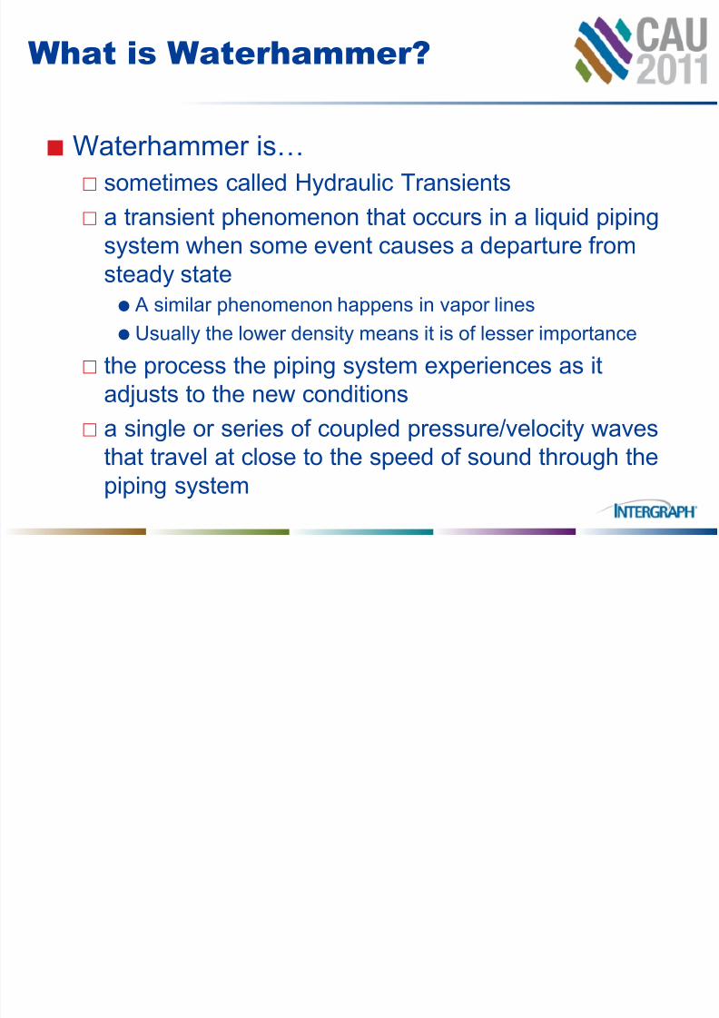
What is Waterhammer?
Waterhammer is…
sometimes called Hydraulic Transients
a transient phenomenon that occurs in a liquid piping
system when some event causes a departure fromsteady state
A similar phenomenon happens in vapor lines
Usually the lower density means it is of lesser importance
the process the piping system experiences as itadjusts to the new conditions
a single or series of coupled pressure/velocity waves
that travel at close to the speed of sound through the
piping system
7/28/2019 CAU2011-PPT-TreyWalters JimWilcox.pptx
http://slidepdf.com/reader/full/cau2011-ppt-treywalters-jimwilcoxpptx 3/34
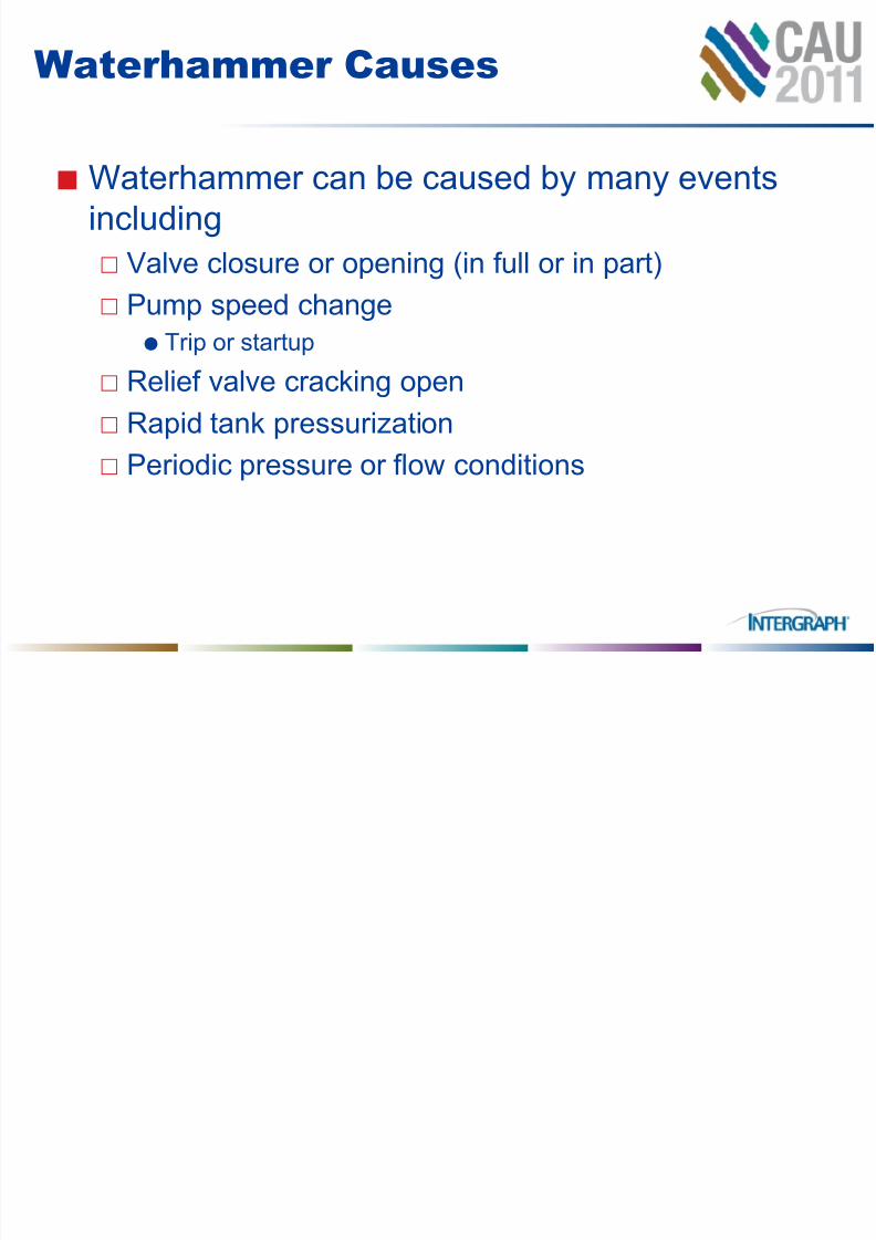
Waterhammer Causes
Waterhammer can be caused by many events
including
Valve closure or opening (in full or in part)
Pump speed change Trip or startup
Relief valve cracking open
Rapid tank pressurization
Periodic pressure or flow conditions
7/28/2019 CAU2011-PPT-TreyWalters JimWilcox.pptx
http://slidepdf.com/reader/full/cau2011-ppt-treywalters-jimwilcoxpptx 4/34
Waterhammer and Force
Imbalances
Waterhammer causes transient force
imbalances in piping systems
This is a result of fast moving pressure waves which
can create temporary force imbalances Elbow pairs are especially susceptible to force
imbalances due to the change in flow direction
Structural supports need to be able to handle
these forces

7/28/2019 CAU2011-PPT-TreyWalters JimWilcox.pptx
http://slidepdf.com/reader/full/cau2011-ppt-treywalters-jimwilcoxpptx 5/34
Waterhammer Video
7/28/2019 CAU2011-PPT-TreyWalters JimWilcox.pptx
http://slidepdf.com/reader/full/cau2011-ppt-treywalters-jimwilcoxpptx 6/34
Waterhammer Software
Waterhammer is a sufficiently complicated
process such that modeling software is usually
required
AFT Impulse™ is a leading waterhammer software
AFT Impulse has been commercially available since
1996
It has been used to model thousands of piping system
transients

7/28/2019 CAU2011-PPT-TreyWalters JimWilcox.pptx
http://slidepdf.com/reader/full/cau2011-ppt-treywalters-jimwilcoxpptx 7/34
Waterhammer Software (2)
Typically the issue of primary interest to the
engineering analyst is understanding transient
pressure extremes
This allows selection of pipe strength and design for equipment protection and general safety
7/28/2019 CAU2011-PPT-TreyWalters JimWilcox.pptx
http://slidepdf.com/reader/full/cau2011-ppt-treywalters-jimwilcoxpptx 8/34
Calculating Force Imbalances
Waterhammer software like AFT Impulse
calculates transient pressures and flows
This information can be used to predict transient
force imbalances
7/28/2019 CAU2011-PPT-TreyWalters JimWilcox.pptx
http://slidepdf.com/reader/full/cau2011-ppt-treywalters-jimwilcoxpptx 9/34
Traditional Force Calculation
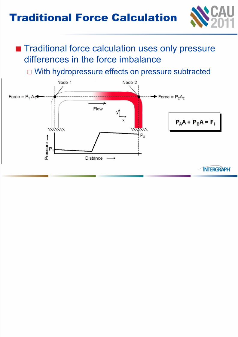
Traditional force calculation uses only pressure
differences in the force imbalance
With hydropressure effects on pressure subtracted
7/28/2019 CAU2011-PPT-TreyWalters JimWilcox.pptx
http://slidepdf.com/reader/full/cau2011-ppt-treywalters-jimwilcoxpptx 10/34
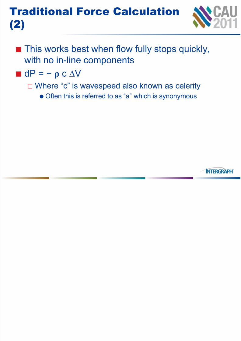
Traditional Force Calculation
(2)
This works best when flow fully stops quickly,
with no in-line components
dP = − ρ c V
Where “c” is wavespeed also known as celerityOften this is referred to as “a” which is synonymous
7/28/2019 CAU2011-PPT-TreyWalters JimWilcox.pptx
http://slidepdf.com/reader/full/cau2011-ppt-treywalters-jimwilcoxpptx 11/34
Traditional Force Calculation
(3)
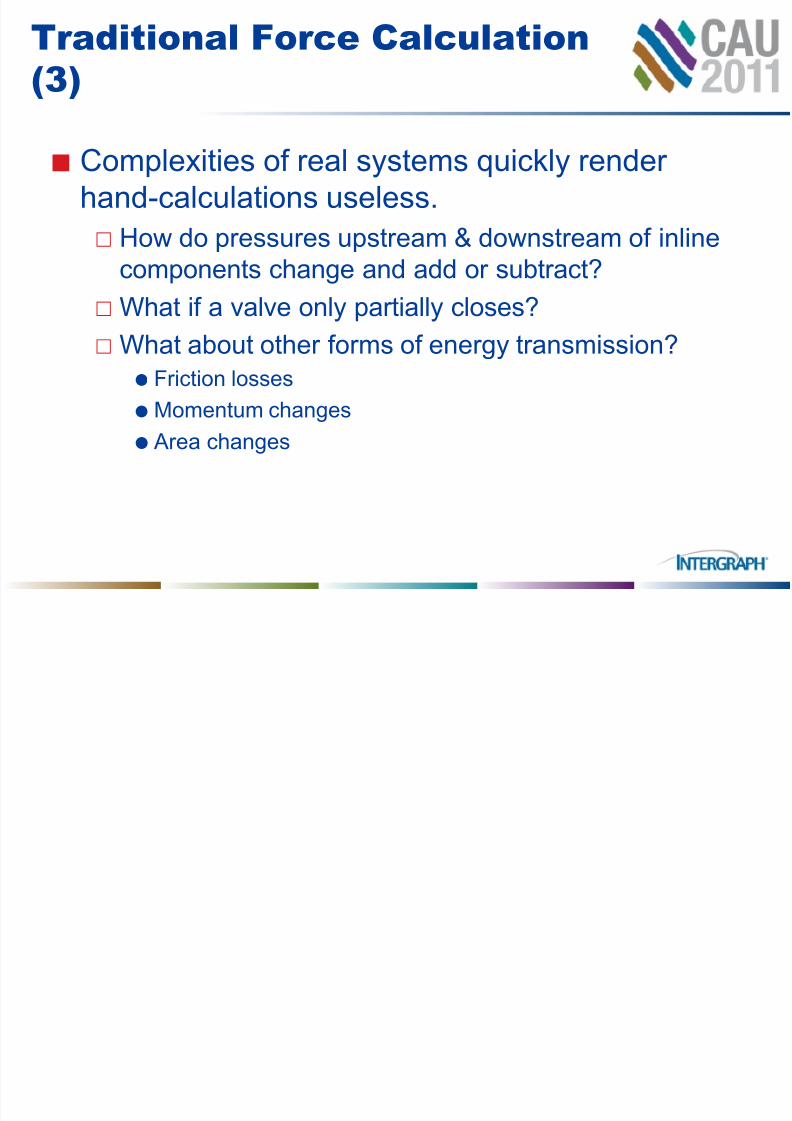
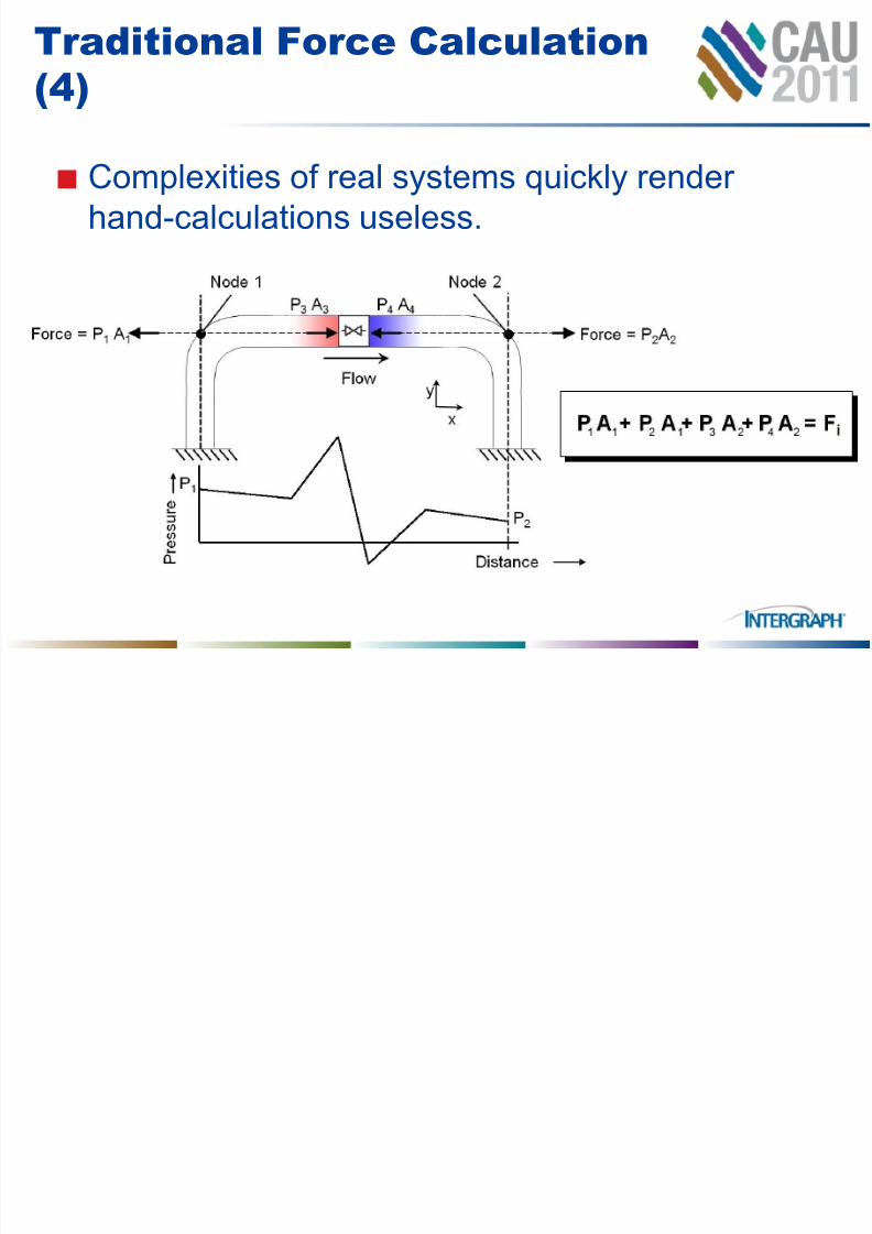
Complexities of real systems quickly render
hand-calculations useless.
How do pressures upstream & downstream of inline
components change and add or subtract? What if a valve only partially closes?
What about other forms of energy transmission?
Friction losses
Momentum changes Area changes
7/28/2019 CAU2011-PPT-TreyWalters JimWilcox.pptx
http://slidepdf.com/reader/full/cau2011-ppt-treywalters-jimwilcoxpptx 12/34
Traditional Force Calculation
(4)
Complexities of real systems quickly render
hand-calculations useless.
7/28/2019 CAU2011-PPT-TreyWalters JimWilcox.pptx
http://slidepdf.com/reader/full/cau2011-ppt-treywalters-jimwilcoxpptx 13/34
Traditional Force Calculation:
Example
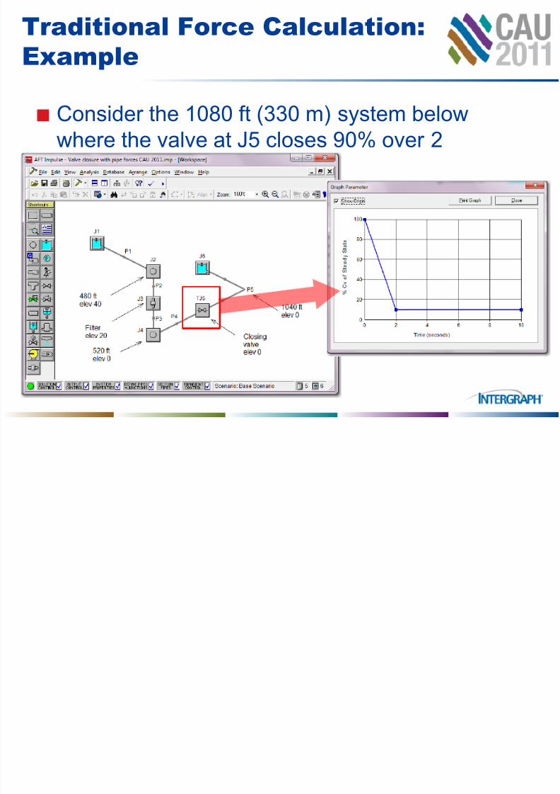
Consider the 1080 ft (330 m) system below
where the valve at J5 closes 90% over 2
seconds
7/28/2019 CAU2011-PPT-TreyWalters JimWilcox.pptx
http://slidepdf.com/reader/full/cau2011-ppt-treywalters-jimwilcoxpptx 14/34
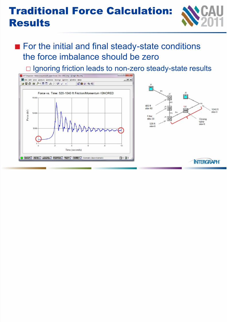
Traditional Force Calculation:
Results
For the initial and final steady-state conditions
the force imbalance should be zero
Ignoring friction leads to non-zero steady-state results

7/28/2019 CAU2011-PPT-TreyWalters JimWilcox.pptx
http://slidepdf.com/reader/full/cau2011-ppt-treywalters-jimwilcoxpptx 15/34
Including Friction
Including all forces including fitting pressure
losses, friction & momentum improves force
calculations
A = πD2/4
Force = PB x AForce = P A x A
Friction & pressure loss forces Other forces + PAA + PBA = 0
Momentum = m A ΔVX,A Momentum = mB ΔVX,B
ΣFfriction + PAA + PBA =
mAΔVX,A - mBΔVX,B
7/28/2019 CAU2011-PPT-TreyWalters JimWilcox.pptx
http://slidepdf.com/reader/full/cau2011-ppt-treywalters-jimwilcoxpptx 16/34
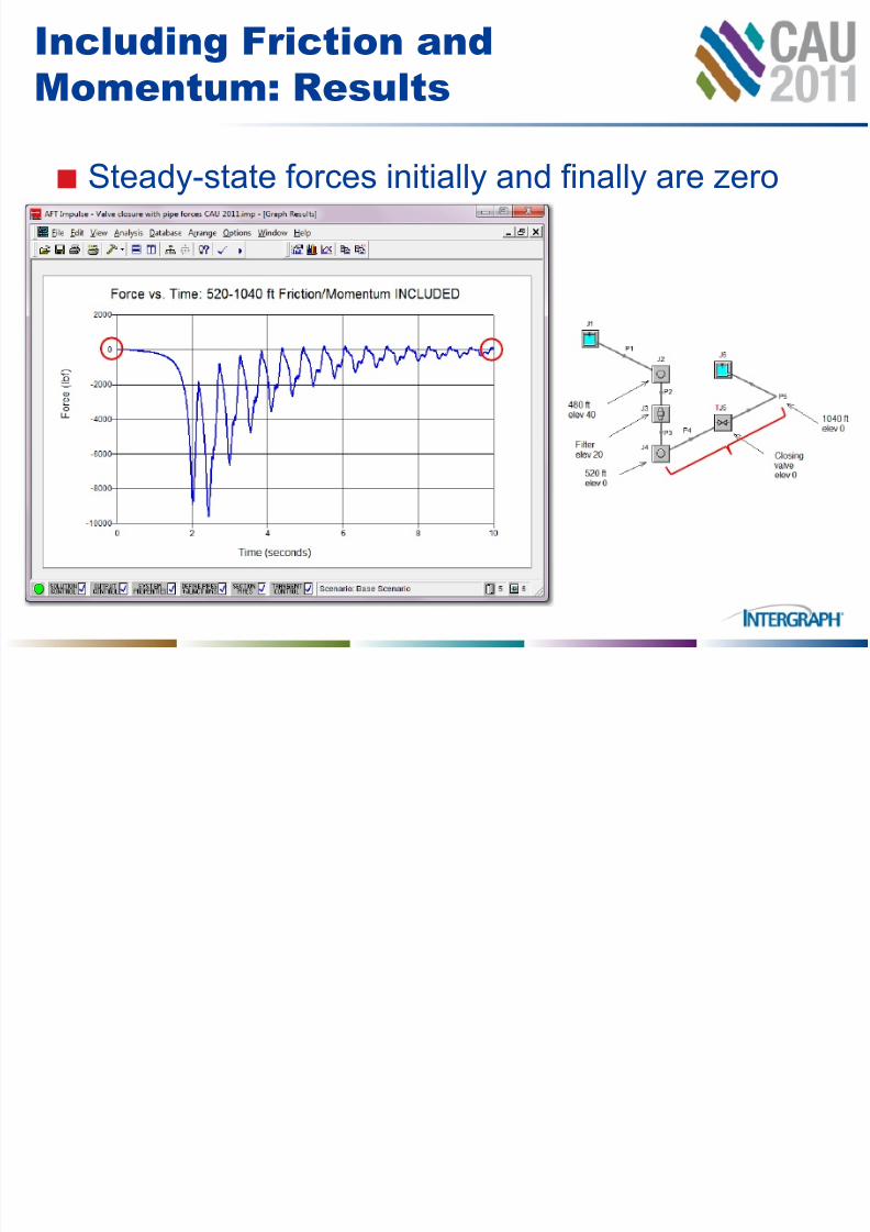
Including Friction and
Momentum: Results
Steady-state forces initially and finally are zero
7/28/2019 CAU2011-PPT-TreyWalters JimWilcox.pptx
http://slidepdf.com/reader/full/cau2011-ppt-treywalters-jimwilcoxpptx 17/34
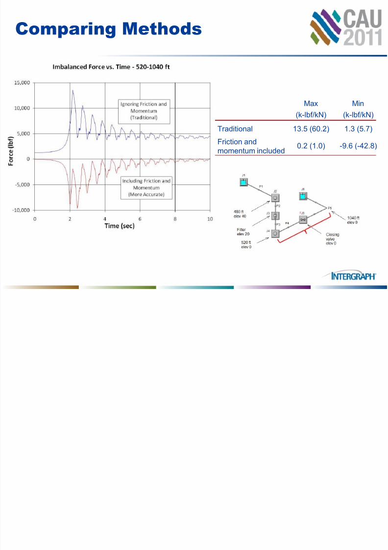
Comparing Methods
Traditional
Friction and
momentum included
Max Min
13.5 (60.2) 1.3 (5.7)
0.2 (1.0) -9.6 (-42.8)
(k-lbf/kN) (k-lbf/kN)
7/28/2019 CAU2011-PPT-TreyWalters JimWilcox.pptx
http://slidepdf.com/reader/full/cau2011-ppt-treywalters-jimwilcoxpptx 18/34
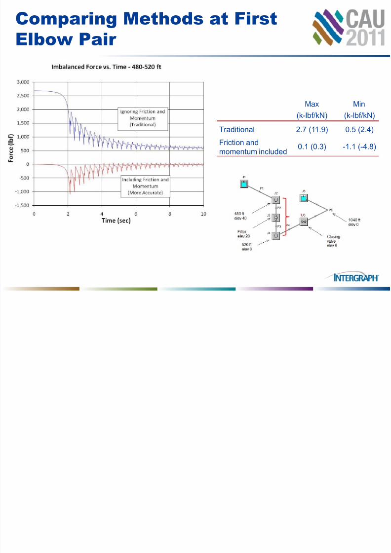
Comparing Methods at First
Elbow Pair
Traditional
Friction and
momentum included
Max Min
2.7 (11.9) 0.5 (2.4)
0.1 (0.3) -1.1 (-4.8)
(k-lbf/kN) (k-lbf/kN)
7/28/2019 CAU2011-PPT-TreyWalters JimWilcox.pptx
http://slidepdf.com/reader/full/cau2011-ppt-treywalters-jimwilcoxpptx 19/34
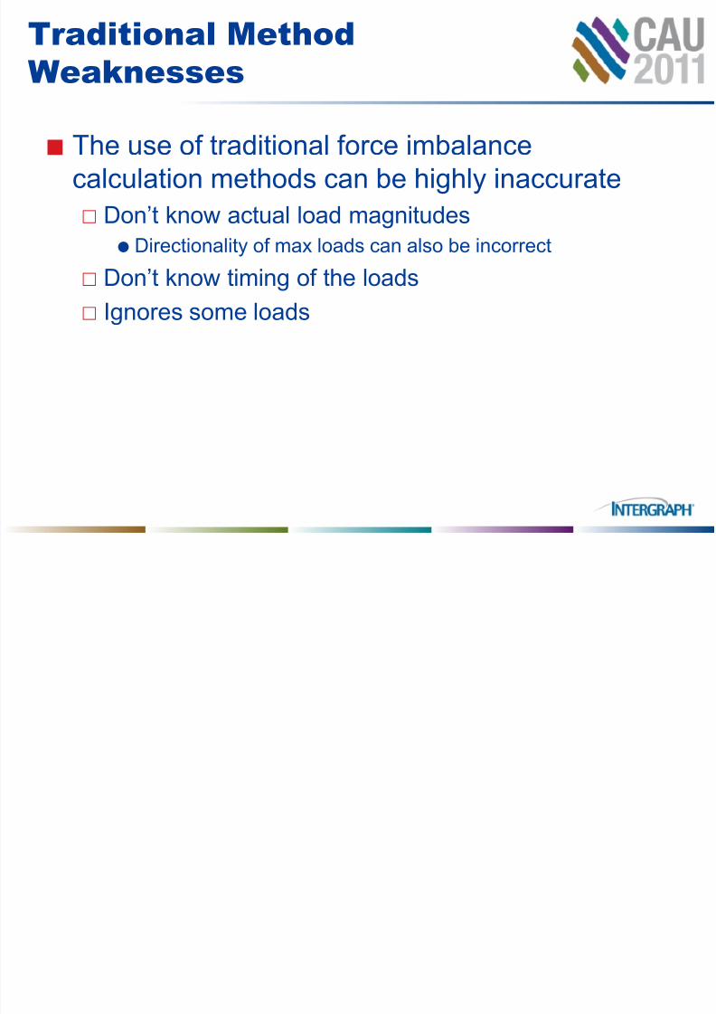
Traditional Method
Weaknesses
The use of traditional force imbalance
calculation methods can be highly inaccurate
Don’t know actual load magnitudes
Directionality of max loads can also be incorrect Don’t know timing of the loads
Ignores some loads
7/28/2019 CAU2011-PPT-TreyWalters JimWilcox.pptx
http://slidepdf.com/reader/full/cau2011-ppt-treywalters-jimwilcoxpptx 20/34
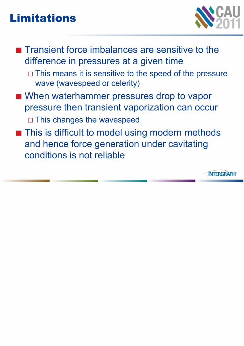
Limitations
Transient force imbalances are sensitive to the
difference in pressures at a given time
This means it is sensitive to the speed of the pressure
wave (wavespeed or celerity) When waterhammer pressures drop to vapor
pressure then transient vaporization can occur
This changes the wavespeed
This is difficult to model using modern methods
and hence force generation under cavitating
conditions is not reliable
7/28/2019 CAU2011-PPT-TreyWalters JimWilcox.pptx
http://slidepdf.com/reader/full/cau2011-ppt-treywalters-jimwilcoxpptx 21/34
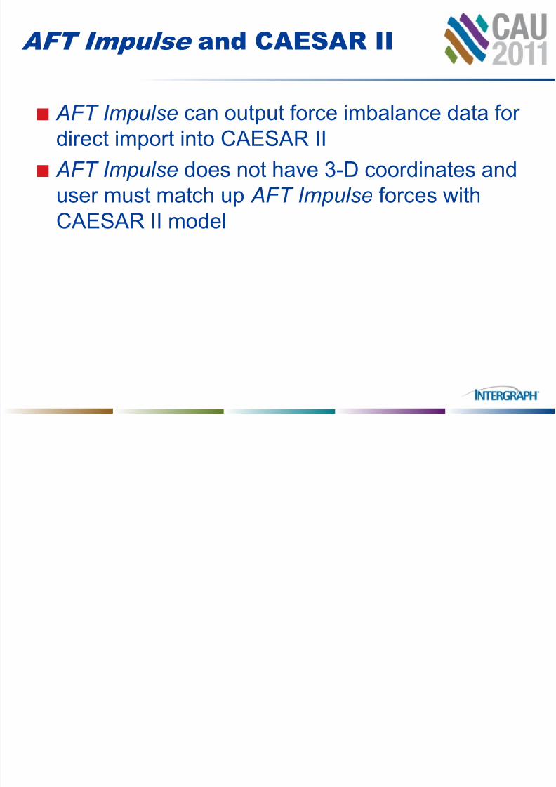
AFT Impulse and CAESAR II
AFT Impulse can output force imbalance data for
direct import into CAESAR II
AFT Impulse does not have 3-D coordinates and
user must match up AFT Impulse forces withCAESAR II model
7/28/2019 CAU2011-PPT-TreyWalters JimWilcox.pptx
http://slidepdf.com/reader/full/cau2011-ppt-treywalters-jimwilcoxpptx 22/34
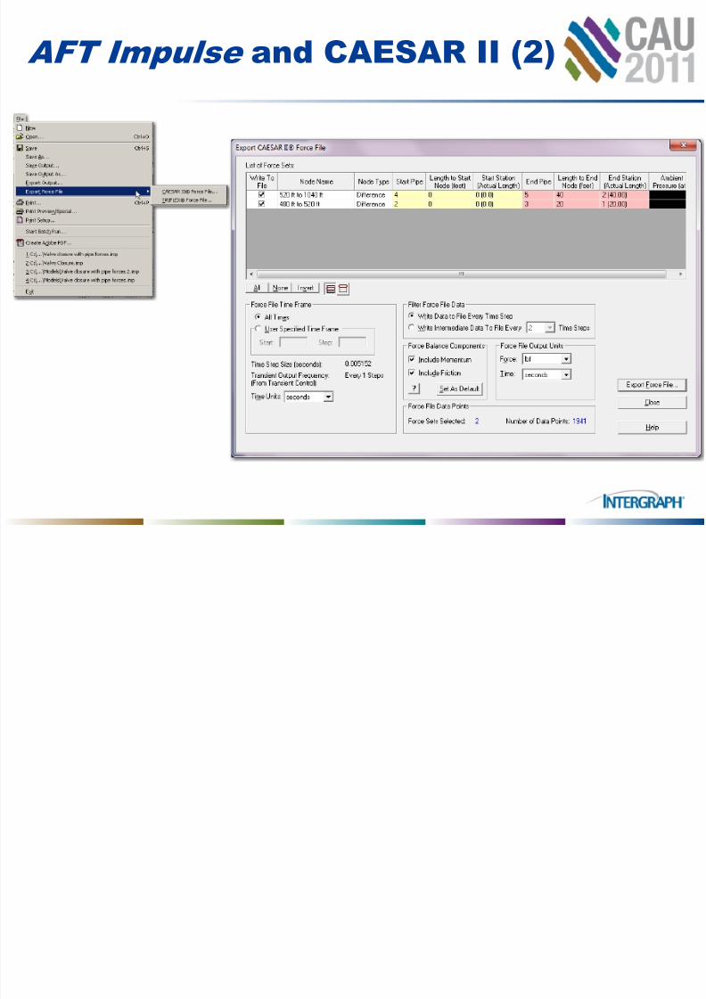
AFT Impulse and CAESAR II (2)
7/28/2019 CAU2011-PPT-TreyWalters JimWilcox.pptx
http://slidepdf.com/reader/full/cau2011-ppt-treywalters-jimwilcoxpptx 23/34
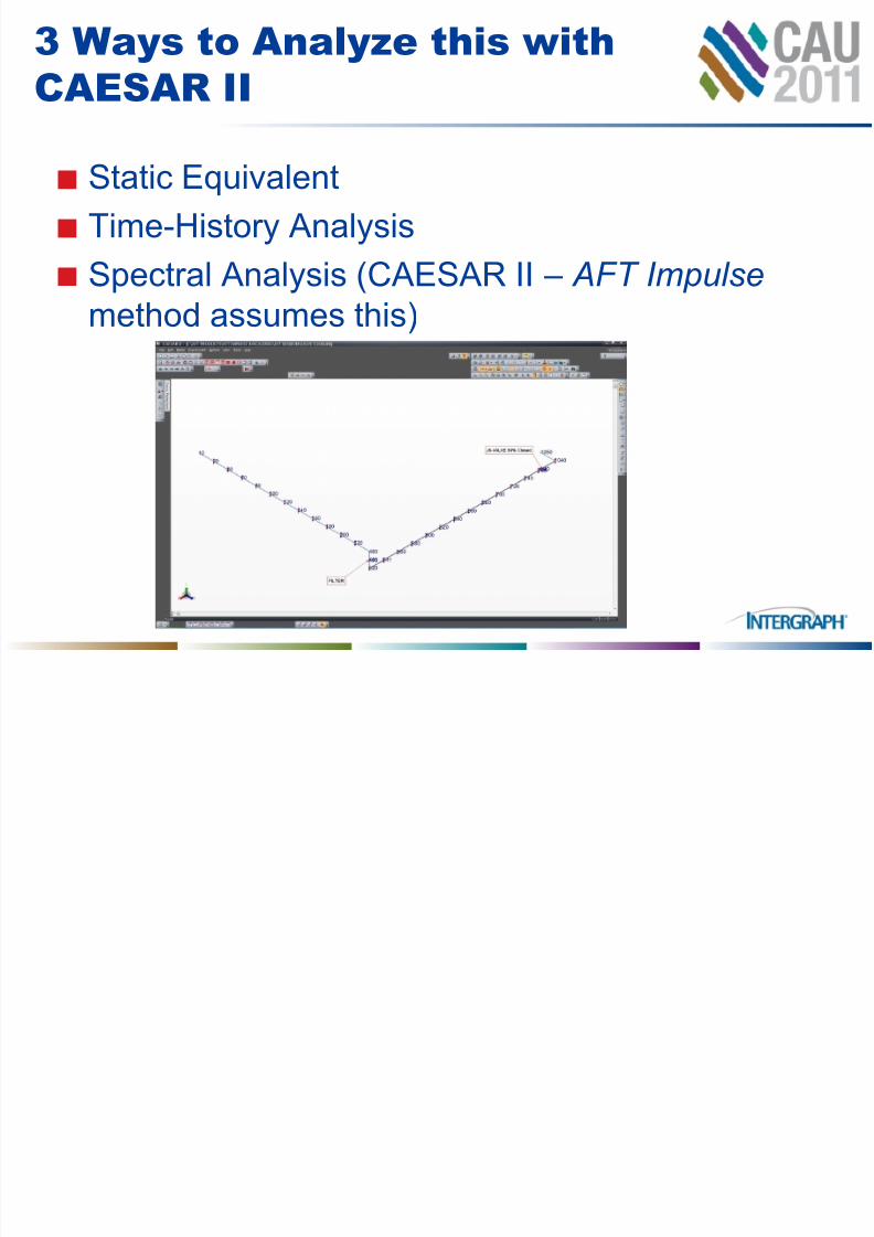
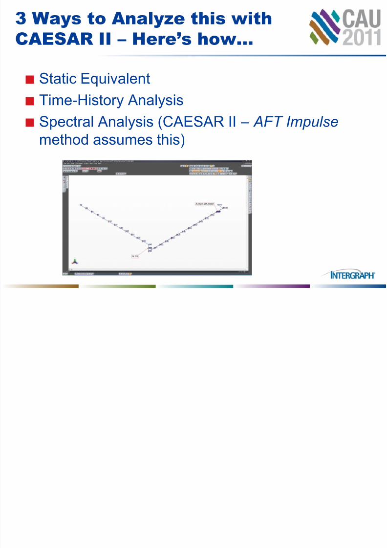
3 Ways to Analyze this with
CAESAR II
Static Equivalent
Time-History Analysis
Spectral Analysis (CAESAR II – AFT Impulse
method assumes this)
7/28/2019 CAU2011-PPT-TreyWalters JimWilcox.pptx
http://slidepdf.com/reader/full/cau2011-ppt-treywalters-jimwilcoxpptx 24/34
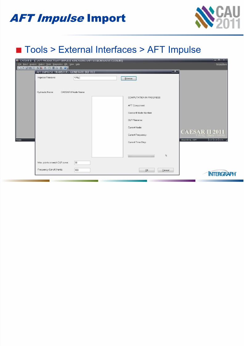
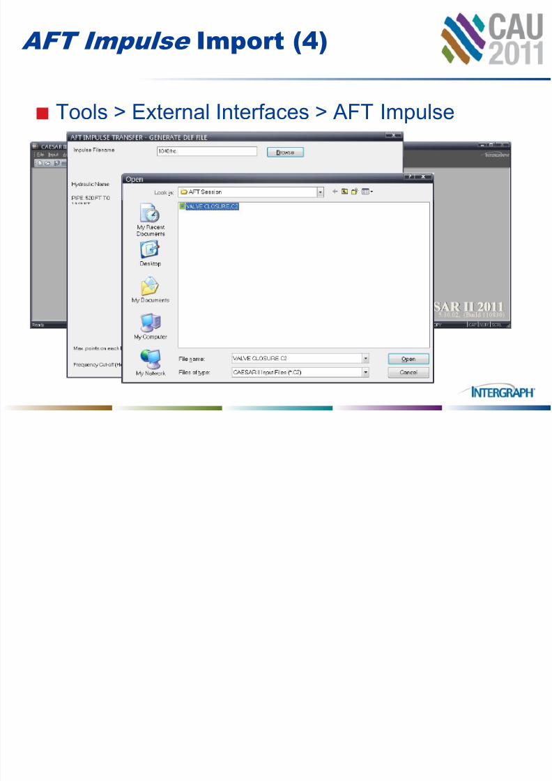
AFT Impulse Import
Tools > External Interfaces > AFT Impulse
7/28/2019 CAU2011-PPT-TreyWalters JimWilcox.pptx
http://slidepdf.com/reader/full/cau2011-ppt-treywalters-jimwilcoxpptx 25/34
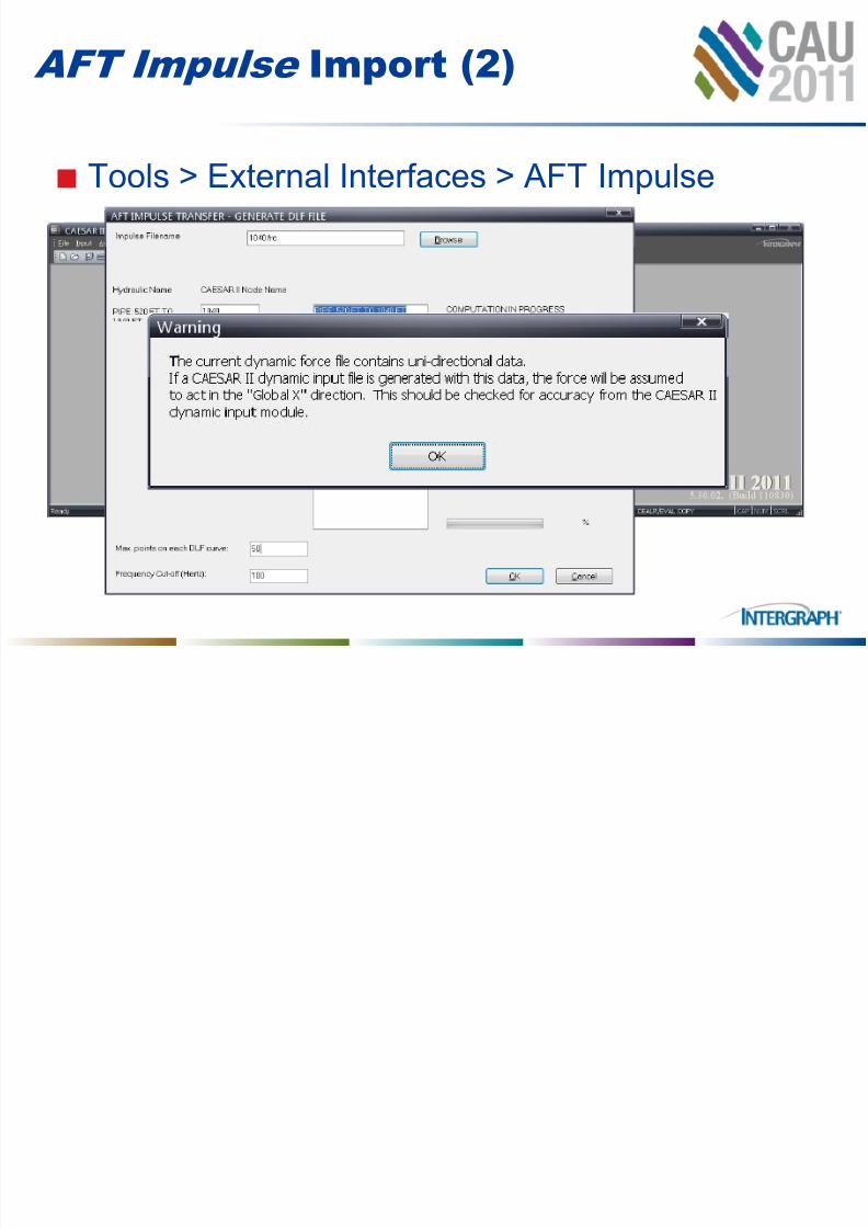
AFT Impulse Import (2)
Tools > External Interfaces > AFT Impulse
7/28/2019 CAU2011-PPT-TreyWalters JimWilcox.pptx
http://slidepdf.com/reader/full/cau2011-ppt-treywalters-jimwilcoxpptx 26/34
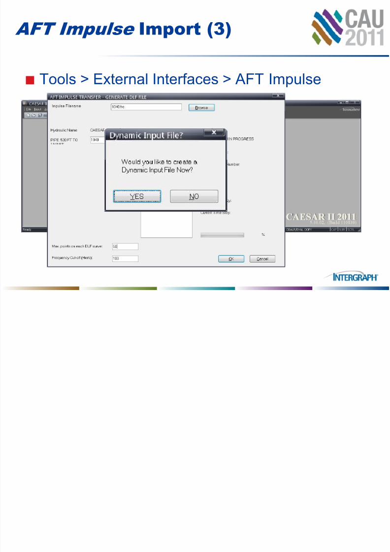
AFT Impulse Import (3)
Tools > External Interfaces > AFT Impulse
7/28/2019 CAU2011-PPT-TreyWalters JimWilcox.pptx
http://slidepdf.com/reader/full/cau2011-ppt-treywalters-jimwilcoxpptx 27/34
AFT Impulse Import (4)
Tools > External Interfaces > AFT Impulse
7/28/2019 CAU2011-PPT-TreyWalters JimWilcox.pptx
http://slidepdf.com/reader/full/cau2011-ppt-treywalters-jimwilcoxpptx 28/34
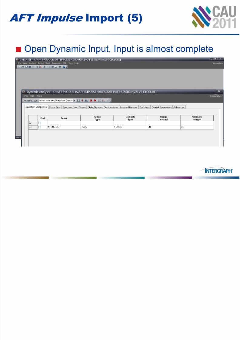
AFT Impulse Import (5)
Open Dynamic Input, Input is almost complete
7/28/2019 CAU2011-PPT-TreyWalters JimWilcox.pptx
http://slidepdf.com/reader/full/cau2011-ppt-treywalters-jimwilcoxpptx 29/34
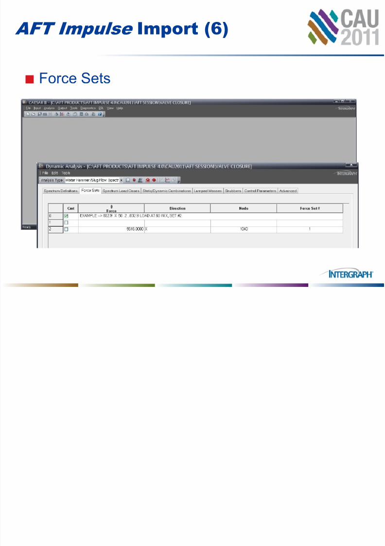
AFT Impulse Import (6)
Force Sets
7/28/2019 CAU2011-PPT-TreyWalters JimWilcox.pptx
http://slidepdf.com/reader/full/cau2011-ppt-treywalters-jimwilcoxpptx 30/34
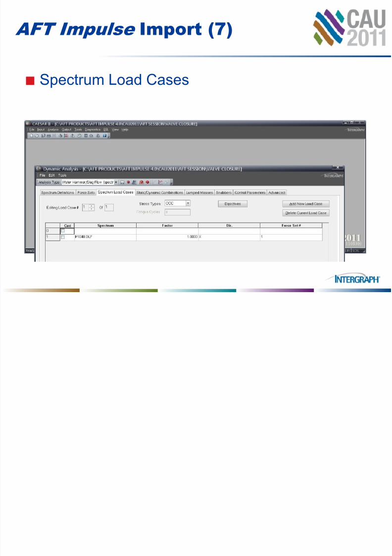
AFT Impulse Import (7)
Spectrum Load Cases
7/28/2019 CAU2011-PPT-TreyWalters JimWilcox.pptx
http://slidepdf.com/reader/full/cau2011-ppt-treywalters-jimwilcoxpptx 31/34
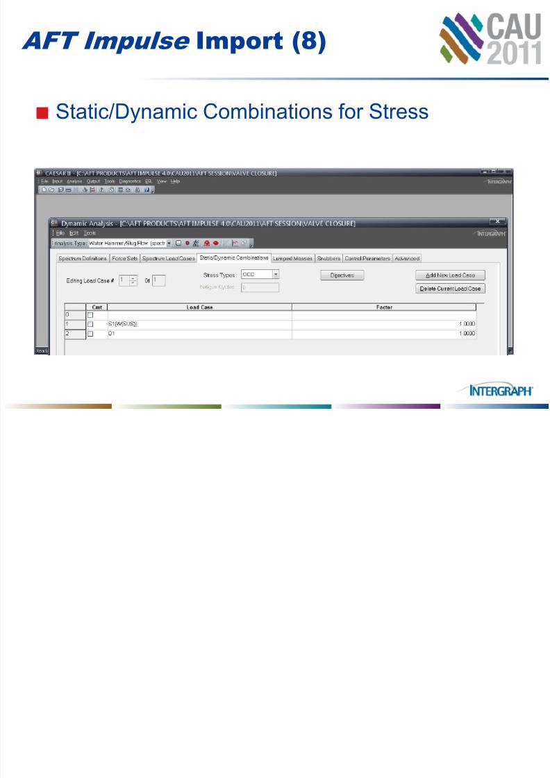
AFT Impulse Import (8)
Static/Dynamic Combinations for Stress
7/28/2019 CAU2011-PPT-TreyWalters JimWilcox.pptx
http://slidepdf.com/reader/full/cau2011-ppt-treywalters-jimwilcoxpptx 32/34
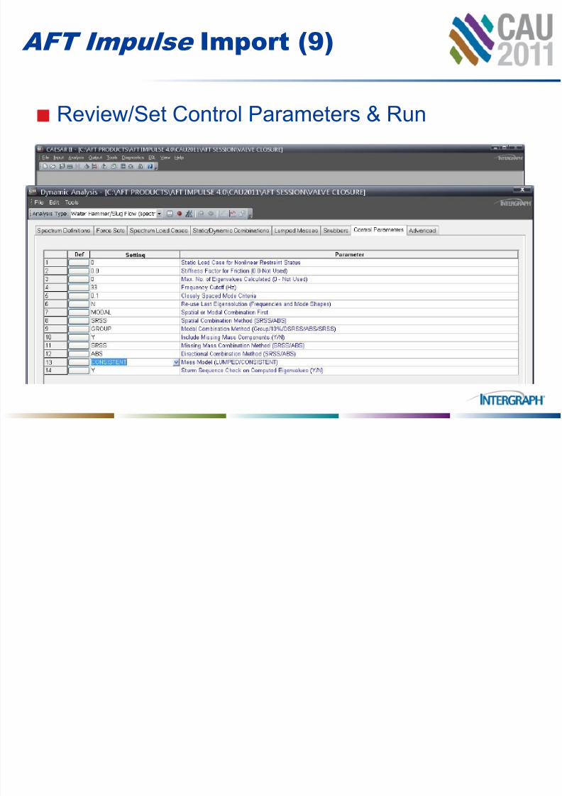
AFT Impulse Import (9)
Review/Set Control Parameters & Run
7/28/2019 CAU2011-PPT-TreyWalters JimWilcox.pptx
http://slidepdf.com/reader/full/cau2011-ppt-treywalters-jimwilcoxpptx 33/34
3 Ways to Analyze this with
CAESAR II – Here’s how…
Static Equivalent
Time-History Analysis
Spectral Analysis (CAESAR II – AFT Impulse
method assumes this)
7/28/2019 CAU2011-PPT-TreyWalters JimWilcox.pptx
http://slidepdf.com/reader/full/cau2011-ppt-treywalters-jimwilcoxpptx 34/34
Conclusions
It is important to model waterhammer events for
proper system design and operation
AFT Impulse can generate transient forces
which can be easily imported into CAESAR II Traditional force estimation techniques which
rely on pressure differences can be highly
inaccurate
Force imbalances in systems with transient
cavitation cannot be reliably predicted because
wavespeeds change