ABSTRACT

System, energy, and flavor dependence of jets through di-hadron correlations in

heavy ion collisions

Christine Nattrass

Yale University

December 2009

QCD predicts a phase transition in nuclear matter at high energy densities. This

matter, called a Quark Gluon Plasma (QGP), should have very different properties

from normal nuclear matter due to its high temperature and density. The Relativistic

Heavy Ion Collider (RHIC) was built to study the QGP. Jets can act as a calibrated

probe to examine the QGP, however, reconstruction of jets in a heavy ion environment

is difficult. Therefore jets have been studied in heavy ion collisions by investigating

the spatial correlations between two intermediate to high-pT hadrons in an event.

Previous studies have shown that the near-side di-hadron correlation peak can be

decomposed into two components, a jet-like correlation and the Ridge. The jet-like

correlation is narrow in both azimuth and pseudorapidity, while the Ridge is narrow

in azimuth but independent of pseudorapidity within STAR’s acceptance. STAR’s

data from Cu+Cu and Au+Au collisions at√sNN = 62 GeV and

√sNN = 200 GeV

allow comparative studies of these components in different systems and at different

energies.

Data on correlations with both identified trigger particles and identified associated

particles are presented, including the first studies of identified particle correlations

in Cu+Cu and the energy dependence of these correlations. The yields are studied

as a function of collision centrality, transverse momentum of the trigger particle,

transverse momentum of the associated particle, and trigger and associated particle

type. The data in this thesis indicate that the jet-like correlation component in heavy

ion collisions is dominantly produced by vacuum fragmentation of hard scattered

partons.

The Ridge component is not present in p+p or d+Au collisions. The Ridge yield

is consistent between systems for the same Npart and has properties similar to the

bulk. Theoretical mechanisms for the production of the Ridge include parton re-

combination, collisional energy loss in the medium (momentum kicks), and gluon

brehmsstrahlung. Comparisons between the expectations of these models and the

data are discussed. The data in this thesis provide key measurements to distinguish

production mechanisms.

System, energy, and flavor dependence of jets through

di-hadron correlations in heavy ion collisions

A Dissertation

Presented to the Faculty of the Graduate School

of

Yale University

in Candidacy for the Degree of

Doctor of Philosophy

By

Christine Nattrass

Dissertation Director: Professor John Harris

December 2009

© Copyright 2009

by

Christine Nattrass

All Rights Reserved

Acknowledgements

Twenty six years ago when I was in day care, I sat on the floor scribbling on a pad of

paper, ripping a sheet of paper off, wadding it up, and throwing it in the trash can.

The staff at the day care came over and asked me what I was doing and I said that

I was writing my dissertation. This thesis has been twenty six years in the making

and many people have helped me along the way.

Many thanks to my parents for their support, encouragement, patience, and toler-

ance. They had to put up with science experiments all over the house - although my

mother’s good canning jars were off limits - and had the creativity to come up with

rules such as, “You can only keep it as a pet if you can identify it,” and, “No eating

while standing on your head.” My mother set a wonderful example for me; many of

the lessons I learned watching her establish herself in psychology as I grew up are

more relevant today in physics than they should be. I got my curiosity and sense

of humor from my father, who taught me how to solder, taught me how to make an

electromagnet, and helped me write my first computer program. Thanks to my older

brother Scott, who never let me take the easy route, and taught me things that he

learned in school - including what our mother termed “bus words.” He has been my

role model, my teacher, my coach, and the best college roommate I ever had. Thanks

to my husband Ondrej, whose support has been invaluable and whose faith in my

abilities has never waivered. It is a very special man who brings his wife chocolate

and extra memory for her computer while she is writing up.

Many people provided company, support, and mentorship throughout my grad-

uate studies - including, in no particular order: Sevil Salur, my Turkish sister, for

unwaivering support, friendship, pan cleaning services, rides, and fun sound effects.

iii

Sevil, I can’t thank you enough for all of your support. Anthony Timmins, mi duck,

for support, physics discussions, last minute plots, friendship, and always being willing

to lend an ear. Astrid Morreale, my friend and co-conspirator - when we work to-

gether, no one can stop us. Anders Knospe for support, friendship, rides, doing dishes,

reaching high shelves, and serving as an excellent guide through New York city. I even

forgive you for Harry Potter. Jana Bielcıkova, for friendship, mentorship, teaching

me how to really program well, and occasional Czech lessons. Latchezar Benetov and

Peter Orth, my second semester quantum field theory study partners, for friendship

and comiseration. Oana Catu, my office mate and partner in crime, for friendship,

help making loud noises, rides, entertainment, and occasional venison. Just no more

police motorcycles, ok? Giorgio Torrieri, for friendship and many, many, many use-

ful physics conversations. Sarah LaPointe, for friendship, plants, chickens, and pigs.

Jaro Bielcık, for friendship and always saying something funny. Betty Abelev - thanks

especially for showing me the tricks to Ξ and Ω reconstruction. Thanks to Monika

Sharma and Sadhana Dash for sari lessons. Thanks to Rashmi Raniwala for Indian

food and Indian cooking lessons and friendship. Thanks to Elena Bruna (who gave

me !), Stephen Baumgart, Richard Witt, Jorn Putschke, Boris Hippolyte, Mark

Heinz, Thomas Ullrich, Xieyue Fan, Jon Gans, Mike Miller, Nikolai Smirnoff, Sofia

Magkiriadou, Jonathan Bouchet, Spiros Margetis, Gene Van Buren, Jerome Lau-

ret, Terry Tarnowsky, Cristina Suarez, Martin Codrington, Michael Daugherity, Jan

Kapitan, Petr Chaloupka, Lee Barnby, Leon Galliard, Marek Bombara, Essam El-

halhuli, George Moschelli, Jason Ulery, Lanny Ray, Jun Takahashi, Fuqiang Wang,

Rene Bellwied, Christina Markert, Marco van Leeuwen, Tim Hallman, Jamie Dunlop,

Bedanga Mohanty, Carla Vale, Sean Gavin, Sergei Voloshin, and Cheuk-yin Wong.

Thanks to the STAR collaboration, the strangeness working group, the high-pT work-

ing group, the jet correlations working group, and the Yale heavy ion group. Thanks

to the RHIC community and the Yale Physics Department - I have been amazed by

the support I’ve received, especially from unexpected sources.

Thanks also to my Roomba and my Scooba, my floor cleaning robots, wedding

gifts from my parents-in-law, and to my dishwasher and my bread machine. Collec-

tively these comprised the army of robots at my command, capable of doing anything

iv

short of writing my thesis. Lindt, Orion, and Figaro deserve special note for having

made my Thesis Chocolate, and thanks to my in-laws for two metric tons of Thesis

Chocolate. Thanks to Saccharomyces cerevisae for the sustainence and entertainment.

Some of my teachers were instrumental in undoing the damage wreaked by others

and these teachers deserve a special thanks. My high school trigonometry teacher,

Mrs. Connie Dotson, reminded me that not only did math not have to be painful

but it actually could be fun, and her nonchalant confidence in my abilities stood in

stark contrast to my math teachers the preceeding three years. My undergraduate

calculus teacher, Dr. Gerald Taylor, reinforced these messages and didn’t even mind

when I limped into class late for the half of a semester when I was on crutches. I

met for the first time with Dr. Richard Eykholt as college sophomore biochemistry

major taking first year physics - the first physics class I’d taken. I told him I wanted

to add a physics major, spend a semester abroad, and still graduate in a total of five

years. Dr. Eykholt, who would become my academic advisor, not only did not laugh

me out of his office but instead helped me draft a plan to do it. I followed that plan

and it eventually led me here, thanks in no small part to his advice and support.

Many thanks to Bonnie Flemming and Meg Urry, both of whom have been in-

valuable mentors and role models. Thanks to Liz Atlas for all of your help. Thanks

to my committee, Richard Easther, Dan McKinsey, Keith Baker, Helen Caines, and

John Harris, for their time and useful comments.

Words cannot convey my graditude towards John Harris, my advisor, and Helen

Caines, my mentor. I really wouldn’t have made it without you. Helen, I hope some

day that I can be as good of a physicist and as good of a person as you are. And I

believe I still owe you a car wash? John, thanks for all of your support and for giving

me so many opportunities to become a better physicist and prove myself. (And sorry

about the exploding root beer!)

v

vi

Contents

Acknowledgements iii

1 Introduction 1

1.1 A new phase of matter . . . . . . . . . . . . . . . . . . . . . . . . . . 1

1.2 The phase diagram of nuclear matter . . . . . . . . . . . . . . . . . . 3

1.3 Phases of the collision . . . . . . . . . . . . . . . . . . . . . . . . . . 6

1.4 Theoretical frameworks to describe heavy ion ccollisions . . . . . . . . 8

1.4.1 Jet quenching models . . . . . . . . . . . . . . . . . . . . . . . 8

1.4.2 The Glasma and the Color Glass Condensate . . . . . . . . . 11

1.4.3 Statistical models . . . . . . . . . . . . . . . . . . . . . . . . . 13

1.4.4 Hydrodynamics . . . . . . . . . . . . . . . . . . . . . . . . . . 15

1.4.5 Recombination . . . . . . . . . . . . . . . . . . . . . . . . . . 22

1.5 Conclusions and overview . . . . . . . . . . . . . . . . . . . . . . . . 24

2 Jets as a probe of a Quark-Gluon Plasma 27

2.1 Studies of jets through high-pT triggered di-hadron correlations . . . 29

2.1.1 Early studies of jets at RHIC . . . . . . . . . . . . . . . . . . 30

2.1.2 The Away-side . . . . . . . . . . . . . . . . . . . . . . . . . . 31

2.1.3 The near-side . . . . . . . . . . . . . . . . . . . . . . . . . . . 33

2.2 Untriggered di-hadron correlations . . . . . . . . . . . . . . . . . . . . 41

2.3 Jet reconstruction . . . . . . . . . . . . . . . . . . . . . . . . . . . . . 42

2.4 Summary . . . . . . . . . . . . . . . . . . . . . . . . . . . . . . . . . 44

vii

3 Experiment 47

3.1 The Relativistic Heavy Ion Collider . . . . . . . . . . . . . . . . . . . 47

3.2 The STAR detector . . . . . . . . . . . . . . . . . . . . . . . . . . . . 49

3.2.1 The Time Projection Chamber . . . . . . . . . . . . . . . . . 53

4 Particle selection and identification 61

4.1 Selection of charged tracks . . . . . . . . . . . . . . . . . . . . . . . . 62

4.2 V 0 reconstruction . . . . . . . . . . . . . . . . . . . . . . . . . . . . . 66

4.3 Ξ and Ω reconstruction . . . . . . . . . . . . . . . . . . . . . . . . . . 74

4.3.1 Ξ reconstruction . . . . . . . . . . . . . . . . . . . . . . . . . 74

4.3.2 Ω reconstruction . . . . . . . . . . . . . . . . . . . . . . . . . 77

5 Correlation Method 81

5.1 Event selection . . . . . . . . . . . . . . . . . . . . . . . . . . . . . . 81

5.2 Correlation technique . . . . . . . . . . . . . . . . . . . . . . . . . . 82

5.2.1 Track merging correction . . . . . . . . . . . . . . . . . . . . . 84

5.3 Separation of the jet-like correlation and the Ridge . . . . . . . . . . 92

5.3.1 Extraction of the jet-like yield . . . . . . . . . . . . . . . . . . 92

5.3.2 Extraction of the Ridge yield . . . . . . . . . . . . . . . . . . 95

6 Results 103

6.1 The jet-like correlation . . . . . . . . . . . . . . . . . . . . . . . . . . 103

6.1.1 Energy and system dependence . . . . . . . . . . . . . . . . . 103

6.1.2 Flavor and system dependence . . . . . . . . . . . . . . . . . . 107

6.2 The Ridge . . . . . . . . . . . . . . . . . . . . . . . . . . . . . . . . . 111

6.2.1 Energy and system dependence . . . . . . . . . . . . . . . . . 111

6.2.2 Flavor dependence . . . . . . . . . . . . . . . . . . . . . . . . 113

6.3 Ω triggered correlations . . . . . . . . . . . . . . . . . . . . . . . . . . 113

6.4 Summary . . . . . . . . . . . . . . . . . . . . . . . . . . . . . . . . . 116

7 Discussion 117

7.1 The jet-like correlation . . . . . . . . . . . . . . . . . . . . . . . . . . 117

viii

7.1.1 Comparisons to PYTHIA . . . . . . . . . . . . . . . . . . . . 119

7.2 The Ridge . . . . . . . . . . . . . . . . . . . . . . . . . . . . . . . . . 124

7.2.1 Theoretical descriptions of the Ridge . . . . . . . . . . . . . . 124

7.2.2 Discussion . . . . . . . . . . . . . . . . . . . . . . . . . . . . . 131

7.2.3 Summary . . . . . . . . . . . . . . . . . . . . . . . . . . . . . 136

8 Conclusions and outlook 137

8.1 Future measurements . . . . . . . . . . . . . . . . . . . . . . . . . . . 138

8.1.1 Studies at√sNN = 200 GeV . . . . . . . . . . . . . . . . . . . 138

8.1.2 Studies of the energy dependence . . . . . . . . . . . . . . . . 141

A Terminology 145

B Geometric cuts 147

B.1 V 0 Geometric Cuts . . . . . . . . . . . . . . . . . . . . . . . . . . . . 147

B.2 Ξ− Geometric Cuts . . . . . . . . . . . . . . . . . . . . . . . . . . . . 153

C Efficiencies 159

C.1 Unidentified hadron efficiencies . . . . . . . . . . . . . . . . . . . . . 159

C.2 V 0 Efficiencies . . . . . . . . . . . . . . . . . . . . . . . . . . . . . . . 160

D Centrality 165

Bibliography 182

ix

x

List of Figures

1.1 QCD coupling constant as a function of energy . . . . . . . . . . . . . 2

1.2 Schematic phase diagram of nuclear matter . . . . . . . . . . . . . . . 3

1.3 Theoretical calculations of the critical point . . . . . . . . . . . . . . 5

1.4 Stages of a heavy ion collision . . . . . . . . . . . . . . . . . . . . . . 6

1.5 Spacetime diagram of a heavy ion collision . . . . . . . . . . . . . . . 7

1.6 Schematic diagram of RAA . . . . . . . . . . . . . . . . . . . . . . . . 9

1.7 Surface bias of single hadrons . . . . . . . . . . . . . . . . . . . . . . 10

1.8 RAA for unidentified hadrons . . . . . . . . . . . . . . . . . . . . . . . 10

1.9 Distribution of gluons as a function of x . . . . . . . . . . . . . . . . 11

1.10 Schematic diagram of the Glasma in a nucleus . . . . . . . . . . . . . 12

1.11 Thermal fits to RHIC data . . . . . . . . . . . . . . . . . . . . . . . . 14

1.12 Diagram showing the location of the reaction plane . . . . . . . . . . 16

1.13 Contours of constant density in a hydrodynamical model . . . . . . . 16

1.14 v2 versus collision energy . . . . . . . . . . . . . . . . . . . . . . . . . 18

1.15 Measured v2 compared to hydrodynamical limits . . . . . . . . . . . . 19

1.16 Particle species dependence of v2 at low-pT . . . . . . . . . . . . . . . 19

1.17 Particle species dependence of v2 at high-pT . . . . . . . . . . . . . . 20

1.18 Comparison of methods for measuring v2 . . . . . . . . . . . . . . . . 21

1.19 Identified particle RCP . . . . . . . . . . . . . . . . . . . . . . . . . . 23

1.20 Cartoon demonstrating recombination . . . . . . . . . . . . . . . . . 24

2.1 Sample di-jet in a p+ p collision at√sNN = 200 GeV . . . . . . . . . 28

2.2 Schematic diagram of a di-jet . . . . . . . . . . . . . . . . . . . . . . 29

2.3 Jet quenching observed in di-hadron correlations . . . . . . . . . . . . 31

xi

2.4 Low-pT correlations . . . . . . . . . . . . . . . . . . . . . . . . . . . . 32

2.5 The punch-through phenomenon . . . . . . . . . . . . . . . . . . . . . 33

2.6 The Ridge in Au+ Au collisions at√sNN = 200 GeV . . . . . . . . . 34

2.7 The Ridge as a function of Npart. . . . . . . . . . . . . . . . . . . . . 35

2.8 The number of particles in the Ridge as a function of ptriggerT . . . . . 36

2.9 Spectra of particles in the Ridge and the jet-like correlation . . . . . 37

2.10 Fragmentation functions with and without Ridge . . . . . . . . . . . 38

2.11 Particle composition of the jet-like correlation and the Ridge . . . . . 39

2.12 Reaction plane dependence of the jet-like correlation and the Ridge . 39

2.13 3-particle correlations on the near-side . . . . . . . . . . . . . . . . . 40

2.14 Di-hadron correlations without pT cuts in Au+Au collisions at√sNN

= 200 GeV . . . . . . . . . . . . . . . . . . . . . . . . . . . . . . . . 41

2.15 Jet spectrum in central Au+ Au collions at√sNN = 200 GeV . . . . 43

3.1 Aerial view of RHIC. . . . . . . . . . . . . . . . . . . . . . . . . . . . 48

3.2 The STAR Detector . . . . . . . . . . . . . . . . . . . . . . . . . . . 50

3.3 Profile of the STAR Detector . . . . . . . . . . . . . . . . . . . . . . 51

3.4 The signal in the ZDC vs the signal in the CTB . . . . . . . . . . . . 52

3.5 The field cage of the TPC . . . . . . . . . . . . . . . . . . . . . . . . 53

3.6 A readout chamber of the TPC . . . . . . . . . . . . . . . . . . . . . 55

3.7 Field lines around a gating grid . . . . . . . . . . . . . . . . . . . . . 56

3.8 Arrangement of the readout modules of the TPC . . . . . . . . . . . 57

3.9 Energy loss per unit length in the STAR TPC. . . . . . . . . . . . . . 58

3.10 An Au+ Au event in the STAR TPC . . . . . . . . . . . . . . . . . . 59

3.11 Vertex resolution in the TPC . . . . . . . . . . . . . . . . . . . . . . 59

3.12 Momentum resolution of the TPC . . . . . . . . . . . . . . . . . . . . 60

4.1 The DCA to the primary vertex for unidentified hadrons. . . . . . . . 63

4.2 The number of TPC hits associated with unidentified hadrons. . . . . 64

4.3 Effective efficiency for reconstructing unidentified hadrons in Cu+Cu

at√sNN = 200 GeV. . . . . . . . . . . . . . . . . . . . . . . . . . . . 64

4.4 Schematic diagram of a V 0 decay. . . . . . . . . . . . . . . . . . . . . 65

xii

4.5 DCA of a V 0 to the primary vertex and of V 0 daughters to each other 67

4.6 pT dependence of the DCA of a V 0 to the primary vertex and of V 0

daughters to each other . . . . . . . . . . . . . . . . . . . . . . . . . . 68

4.7 DCA of Λ daughters to the primary vertex and decay length versus the

reconstructed mass . . . . . . . . . . . . . . . . . . . . . . . . . . . . 69

4.8 DCA of V 0 to primary vertex and of V 0 daughters to each other . . . 71

4.9 V 0 mass widths. . . . . . . . . . . . . . . . . . . . . . . . . . . . . . . 72

4.10 V 0 mass peak centers. . . . . . . . . . . . . . . . . . . . . . . . . . . 72

4.11 V 0 purity. . . . . . . . . . . . . . . . . . . . . . . . . . . . . . . . . . 73

4.12 Effective V 0 reconstruction efficiency. . . . . . . . . . . . . . . . . . . 73

4.13 Ξ DCA of Λ to primary vertex versus DCA of Ξ to primary vertex. . 75

4.14 Ξ mass peak with and without correlated cut . . . . . . . . . . . . . . 76

4.15 Centers of Ξ mass peaks. . . . . . . . . . . . . . . . . . . . . . . . . . 77

4.16 Ξ center. . . . . . . . . . . . . . . . . . . . . . . . . . . . . . . . . . . 78

4.17 Ω mass peaks. . . . . . . . . . . . . . . . . . . . . . . . . . . . . . . . 79

5.1 Distributions of tracks in φ and η . . . . . . . . . . . . . . . . . . . . 84

5.2 Sample track pair efficiency in ∆φ and ∆η . . . . . . . . . . . . . . . 85

5.3 Location of the track merging dips at small ∆φ and small ∆η in h-h

correlations . . . . . . . . . . . . . . . . . . . . . . . . . . . . . . . . 86

5.4 Correction for track merging dips in h-h correlations . . . . . . . . . . 89

5.5 Location of the track merging dips at small ∆φ and small ∆η in V 0-h

correlations . . . . . . . . . . . . . . . . . . . . . . . . . . . . . . . . 90

5.6 Location of the track merging dips at small ∆φ and small ∆η in Ξ-h

correlations . . . . . . . . . . . . . . . . . . . . . . . . . . . . . . . . 91

5.7 Location of the track merging dips at small ∆φ and small ∆η in h-V 0

correlations . . . . . . . . . . . . . . . . . . . . . . . . . . . . . . . . 92

5.8 Sample acceptance corrected correlation . . . . . . . . . . . . . . . . 93

5.9 Sample jet-like correlations using ∆φ and ∆η methods . . . . . . . . 96

5.10 v2 in Cu+ Cu collisions at√sNN = 62 GeV . . . . . . . . . . . . . . 98

5.11 v2 in Cu+ Cu collisions at√sNN = 200 GeV . . . . . . . . . . . . . 99

xiii

5.12 v2 in Au+ Au collisions at√sNN = 62 GeV . . . . . . . . . . . . . . 99

5.13 Sample correlations in ∆φ showing background . . . . . . . . . . . . 101

6.1 ptriggerT dependence of YJet for unidentified hadrons for

√sNN = 62 GeV

and√sNN = 200 GeV . . . . . . . . . . . . . . . . . . . . . . . . . . 104

6.2 passociatedT dependence of YJet for unidentified hadrons for

√sNN = 62

GeV and√sNN = 200 GeV . . . . . . . . . . . . . . . . . . . . . . . 105

6.3 Npart dependence of YJet for inidentified hadrons for√sNN = 62 GeV

and√sNN = 200 GeV . . . . . . . . . . . . . . . . . . . . . . . . . . 105

6.4 Collision energy and system size dependence of widths for unidentified

hadrons . . . . . . . . . . . . . . . . . . . . . . . . . . . . . . . . . . 106

6.5 ptriggerT dependence of YJet for identified trigger particles . . . . . . . . 108

6.6 passociatedT dependence of YJet for identified trigger particles . . . . . . 109

6.7 Npart dependence of YJet for identified trigger particles . . . . . . . . 109

6.8 ptriggerT dependence of YJet for identified associated particles . . . . . . 110

6.9 passociatedT dependence of YJet for identified associated particles . . . . 111

6.10 Npart dependence of YRidge for unidentified hadrons for√sNN = 62

GeV and√sNN = 200 GeV . . . . . . . . . . . . . . . . . . . . . . . 112

6.11 Npart dependence of YRidge/YJet for unidentified hadrons for√sNN =

62 GeV and√sNN = 200 GeV . . . . . . . . . . . . . . . . . . . . . . 112

6.12 Npart dependence of YRidge for identified trigger particles . . . . . . . 113

6.13 Ω triggered correlations for different passociatedT cuts . . . . . . . . . . . 114

6.14 Ω triggered correlations for different ptriggerT cuts . . . . . . . . . . . . 115

6.15 Ω triggered correlations for different geometric cuts . . . . . . . . . . 115

7.1 Comparison of inclusive Λ+Λ2K0

S

to that in the jet-like correlation and the

Ridge in Cu+ Cu and Au+ Au collisions at√sNN = 200 GeV . . . 118

7.2 ptriggerT dependence of YJet for

√sNN = 62 GeV and

√sNN = 200 GeV

compared to PYTHIA . . . . . . . . . . . . . . . . . . . . . . . . . . 120

7.3 passociatedT dependence of YJet for

√sNN = 62 GeV and

√sNN = 200

GeV compared to PYTHIA . . . . . . . . . . . . . . . . . . . . . . . 121

xiv

7.4 Npart dependence of YJet for√sNN = 62 GeV and

√sNN = 200 GeV

compared to PYTHIA . . . . . . . . . . . . . . . . . . . . . . . . . . 122

7.5 Collision energy and system size dependence of widths compared to

PYTHIA . . . . . . . . . . . . . . . . . . . . . . . . . . . . . . . . . . 123

7.6 Schematic diagram depicting the radial flow plus trigger bias model . 124

7.7 Di-hadron correlation predicted in the radial flow plus trigger bias model125

7.8 Di-hadron correlation predicted in the radial flow plus trigger bias model126

7.9 The Ridge produced in a Color Glass Condensate . . . . . . . . . . . 127

7.10 Schematic diagram showing the mechanism for momentum kick model. 129

7.11 Collision energy dependence in the Momentum Kick model . . . . . . 130

7.12 Rapidity dependence of the Ridge yield in the Momentum Kick Model 130

7.13 Ridge production through radiated gluons broadened by transverse flow131

7.14 Broadening of the jet-like correlation from plasma instabilities . . . . 132

8.1 Separation of particles in STAR TOF . . . . . . . . . . . . . . . . . . 140

8.2 Di-hadron correlations in PYTHIA for RHIC beam energy scan energies142

A.1 Rapidity and pseudorapidity . . . . . . . . . . . . . . . . . . . . . . . 146

xv

xvi

List of Tables

3.1 Collision systems and energies at RHIC . . . . . . . . . . . . . . . . . 48

3.2 RHIC design specifications . . . . . . . . . . . . . . . . . . . . . . . . 49

4.1 Properties of the Λ, K0S, Ξ−, and Ω− . . . . . . . . . . . . . . . . . . 62

4.2 Default geometric cuts for V 0s . . . . . . . . . . . . . . . . . . . . . . 67

4.3 V 0 center parameters . . . . . . . . . . . . . . . . . . . . . . . . . . . 70

4.4 Default geometric cuts for Ξ and Ω . . . . . . . . . . . . . . . . . . . 74

4.5 Ξ center parameters . . . . . . . . . . . . . . . . . . . . . . . . . . . . 76

4.6 Cut sets for Ω candidates . . . . . . . . . . . . . . . . . . . . . . . . . 79

5.1 Parameters from fits of v2 in Cu + Cu collisions at√sNN = 62 GeV

and√sNN = 200 GeV . . . . . . . . . . . . . . . . . . . . . . . . . . 98

5.2 Parameters from fits of v2 in Au+ Au collisions at√sNN = 62 GeV . 100

6.1 Inverse slope parameter of passociatedT for unidentified hadrons . . . . . 104

6.2 Inverse slope parameter k (MeV/c) of passociatedT for identified associated

particles . . . . . . . . . . . . . . . . . . . . . . . . . . . . . . . . . . 110

8.1 Number of events proposed for the RHIC beam energy scan compared

to the number of events needed for studies of the Ridge . . . . . . . . 143

B.1 Geometric cuts for Λ . . . . . . . . . . . . . . . . . . . . . . . . . . . 147

B.2 Geometric cuts for K0S . . . . . . . . . . . . . . . . . . . . . . . . . . 150

B.3 Geometric cuts for Ξ . . . . . . . . . . . . . . . . . . . . . . . . . . . 153

xvii

C.1 Parameters from efficiency fits for unidentified hadrons in Au + Au

collisions at√sNN = 62 GeV . . . . . . . . . . . . . . . . . . . . . . 159

C.2 Parameters from efficiency fits for unidentified hadrons in Cu + Cu

collisions at√sNN = 62 GeV . . . . . . . . . . . . . . . . . . . . . . 160

C.3 Parameters from efficiency fits for unidentified hadrons in Cu + Cu

collisions at√sNN = 200 GeV . . . . . . . . . . . . . . . . . . . . . . 160

C.4 Parameters from efficiency fits for Λ baryons in Cu+ Cu collisions at√sNN = 200 GeV . . . . . . . . . . . . . . . . . . . . . . . . . . . . . 160

C.5 Parameters from efficiency fits for Λ baryons in Cu+ Cu collisions at√sNN = 200 GeV . . . . . . . . . . . . . . . . . . . . . . . . . . . . . 161

C.6 Parameters from efficiency fits for K0S baryons in Cu+Cu collisions at

√sNN = 200 GeV . . . . . . . . . . . . . . . . . . . . . . . . . . . . . 162

D.1 Centrality definitions for Cu+ Cu collisions at√sNN = 62 GeV . . . 165

D.2 Centrality definitions for Cu+ Cu collisions at√sNN = 200 GeV . . 165

D.3 Centrality definitions for Au+ Au collisions at√sNN = 62 GeV . . . 166

xviii

Chapter 1

Introduction

1.1 A new phase of matter

The most successful theory for explaining the behavior of nuclear matter so far is

Quantum ChromoDynamics (QCD), and fundamental attributes of QCD indicate

that there is a new phase of nuclear matter at high energy densities. Figure 1.1

shows the QCD coupling constant αs as a function of the momentum transfer, Q.

Unlike Quantum ElectroDynamics (QED), the coupling constant in QCD is large

at low momentum transfer and perturbative calculations do not converge. A direct

consequence of the energy dependence of the coupling constant is asymptotic freedom,

which a Nobel prize was awarded for in 2004. Unlike the macroscopic forces we are

familiar with, the strong force is weaker at very short distances (largeQ2) than at large

distances (small Q2). As a consequence, if bound quarks are separated, it eventually

becomes energetically favorable to create a new quark-antiquark pair rather than to

continue moving the quarks farther apart. Hence free quarks are not observed in

nature. The QCD analog to electric charge in QED is color charge, which carries the

strong force. Only color neutral states, the color singlets, can exist as stable nuclear

matter at normal densities.

However, when quarks are close together, the attraction between individual quarks

is weak. T. D. Lee proposed in 1974 that quarks and gluons could therefore be created

in a state where they would behave as if they were free within the bounds of the

1

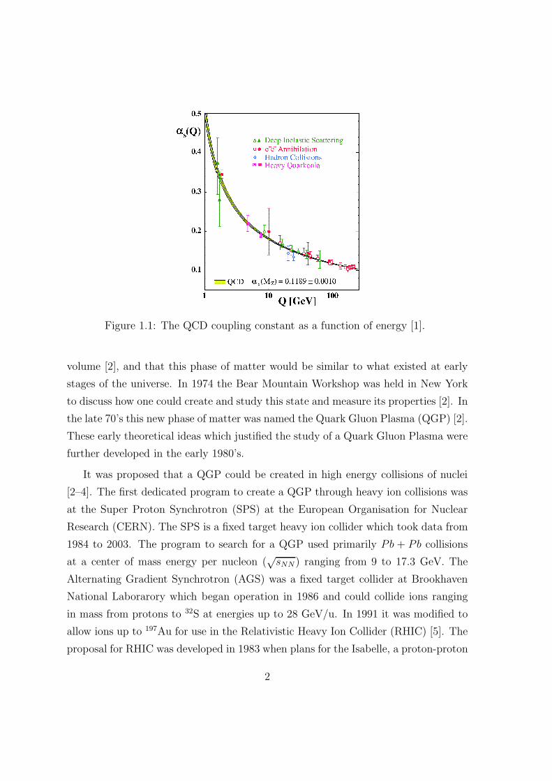
Figure 1.1: The QCD coupling constant as a function of energy [1].

volume [2], and that this phase of matter would be similar to what existed at early

stages of the universe. In 1974 the Bear Mountain Workshop was held in New York

to discuss how one could create and study this state and measure its properties [2]. In

the late 70’s this new phase of matter was named the Quark Gluon Plasma (QGP) [2].

These early theoretical ideas which justified the study of a Quark Gluon Plasma were

further developed in the early 1980’s.

It was proposed that a QGP could be created in high energy collisions of nuclei

[2–4]. The first dedicated program to create a QGP through heavy ion collisions was

at the Super Proton Synchrotron (SPS) at the European Organisation for Nuclear

Research (CERN). The SPS is a fixed target heavy ion collider which took data from

1984 to 2003. The program to search for a QGP used primarily Pb + Pb collisions

at a center of mass energy per nucleon (√sNN ) ranging from 9 to 17.3 GeV. The

Alternating Gradient Synchrotron (AGS) was a fixed target collider at Brookhaven

National Laborarory which began operation in 1986 and could collide ions ranging

in mass from protons to 32S at energies up to 28 GeV/u. In 1991 it was modified to

allow ions up to 197Au for use in the Relativistic Heavy Ion Collider (RHIC) [5]. The

proposal for RHIC was developed in 1983 when plans for the Isabelle, a proton-proton

2

crossover

1

0.1

T, GeV

0 µB, GeV

pointcritical

matterphases

quark

CFLnuclearmattervacuum

hadron gas

QGP

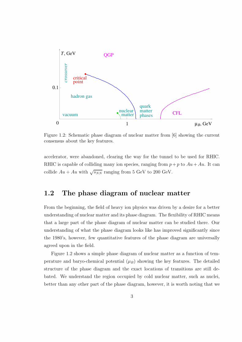
Figure 1.2: Schematic phase diagram of nuclear matter from [6] showing the currentconsensus about the key features.

accelerator, were abandoned, clearing the way for the tunnel to be used for RHIC.

RHIC is capable of colliding many ion species, ranging from p+ p to Au+Au. It can

collide Au+ Au with√sNN ranging from 5 GeV to 200 GeV.

1.2 The phase diagram of nuclear matter

From the beginning, the field of heavy ion physics was driven by a desire for a better

understanding of nuclear matter and its phase diagram. The flexibility of RHIC means

that a large part of the phase diagram of nuclear matter can be studied there. Our

understanding of what the phase diagram looks like has improved significantly since

the 1980’s, however, few quantitative features of the phase diagram are universally

agreed upon in the field.

Figure 1.2 shows a simple phase diagram of nuclear matter as a function of tem-

perature and baryo-chemical potential (µB) showing the key features. The detailed

structure of the phase diagram and the exact locations of transitions are still de-

bated. We understand the region occupied by cold nuclear matter, such as nuclei,

better than any other part of the phase diagram, however, it is worth noting that we

3

still have an incomplete understanding of even the proton. The proton’s spin cannot

be explained by the spin of its valence quarks alone, and the contributions of gluons

and the orbital momentum are still being measured [7]. We know that cool nuclear

matter at moderate densities exists at a µB of about 1 GeV, meaning that it takes a

little more than 1 GeV to add a baryon to the system [6].

At moderate densities and low temperatures, there are ordered phases of cold

quark matter, similar to the various phases of ice [6]. At somewhat higher densities

nuclear matter is expected to be color-flavor locked, meaning that the quarks are ex-

pected to form Cooper pairs, coupling is expected to be weak, and strong correlations

between flavor and color are expected. This matter is expected to behave as a color

superconductor [8]. Nuclear matter at these densities is not directly experimentally

accessible, however, the matter in the center of neutron stars may occupy this region

of the phase diagram.

We know that if we heat nuclear matter at densities comparable to those found

in nuclei to moderate temperatures, it forms a hadron gas, comprising low mass

baryons and mesons made of mostly u and d quarks. At higher temperatures we

expect a quark-gluon plasma, characterized by both chiral symmetry restoration and

free quarks and gluons. At baryo-chemical potentials at and below those of normal

nuclear matter we therefore expect a phase transition from a hadron gas to a quark-

gluon plasma.

The question of the order of the phase transition has been the subject of much

debate. Predictions have been made by lattice QCD. An approximation is made that

space can be discretized, making calculations in the non-perturbative regime of QCD

possible. Lattice simulations indicate that for µB = 0, the transition is a crossover

rather than a phase transition [9]. This means that the hadron gas and the QGP

coexist. A similar crossover transition exists for water. At high temperature and

pressure, the density of water decreases and the density of water vapor increases,

making the two phases indistinguishable. Similarly, the density of the hadron gas is

high and the density of the QGP is low in the crossover region, making the phases

indistinguishable.

Lattice calculations for µB = 0 converge, however, at µB 6= 0 lattice calculations

4

CO94

NJL01NJL89b

CJT02

NJL89a

LR04

RM98

LSM01

HB02 LTE03LTE04

3NJL05

INJL98

LR01

PNJL06

130

9

5

2

17

50

0

100

150

200

0 400 800 1000 1200 1400 1600600200

T ,MeV

µB, MeV

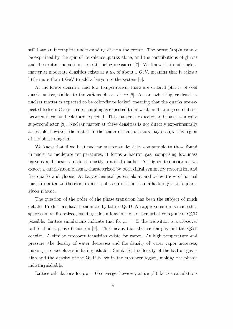
Figure 1.3: Model predictions for the location of the critical point from [6]. Blackpoints are predictions from extrapolations from lattice calculations at µB = 0, greenpoints are lattice predictions, and red circles are the chemical freezeout points forheavy ion collisions at the

√sNN indicated by the point. Dashed lines correspond

to extrapolations of the transition point at µB = 0 using different estimations of the

slopedT

dµ2B

at µB = 0.

do not reliably converge so it is more difficult to make definitive statements [6]. For

larger µB, evidence points towards a first order phase transition [10]. This would

mean there must be a critical point. This would be a tricritical point where confined

nuclear matter and the QGP meet if chiral symmetry has been restored and the u

and d quarks can be considered massless [11].

The location of the tricritical point has been calculated by making assumptions

about how to extrapolate to finite µB from µB = 0, and these calculations are based

on models rather than being solidly rooted in QCD [6]. Figure 1.3 shows model pre-

dictions for the location of the tricritical point, demonstrating that there is still no

consensus. There is therefore no consensus on the location of the line corresponding to

the first order phase transition, although more recent calculations are in better agree-

ment than earlier calculations. The matter produced at RHIC is generally believed

5

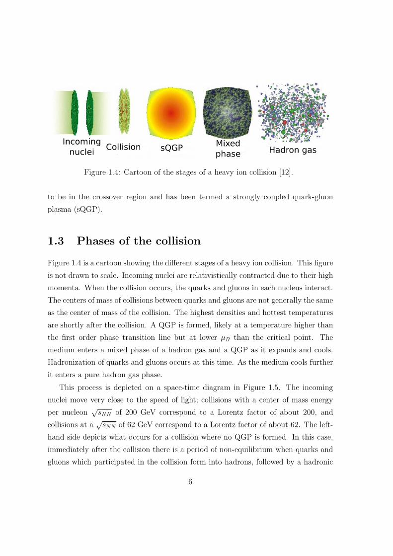
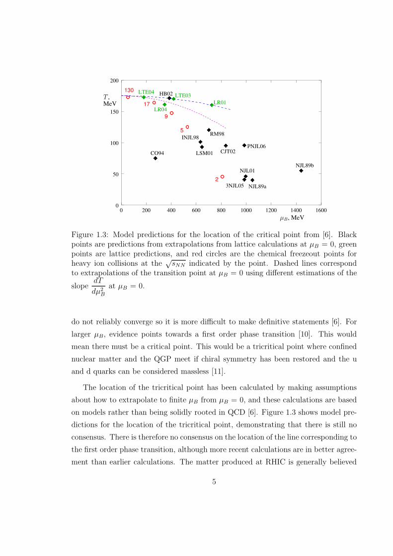
Figure 1.4: Cartoon of the stages of a heavy ion collision [12].

to be in the crossover region and has been termed a strongly coupled quark-gluon

plasma (sQGP).

1.3 Phases of the collision

Figure 1.4 is a cartoon showing the different stages of a heavy ion collision. This figure

is not drawn to scale. Incoming nuclei are relativistically contracted due to their high

momenta. When the collision occurs, the quarks and gluons in each nucleus interact.

The centers of mass of collisions between quarks and gluons are not generally the same

as the center of mass of the collision. The highest densities and hottest temperatures

are shortly after the collision. A QGP is formed, likely at a temperature higher than

the first order phase transition line but at lower µB than the critical point. The

medium enters a mixed phase of a hadron gas and a QGP as it expands and cools.

Hadronization of quarks and gluons occurs at this time. As the medium cools further

it enters a pure hadron gas phase.

This process is depicted on a space-time diagram in Figure 1.5. The incoming

nuclei move very close to the speed of light; collisions with a center of mass energy

per nucleon√sNN of 200 GeV correspond to a Lorentz factor of about 200, and

collisions at a√sNN of 62 GeV correspond to a Lorentz factor of about 62. The left-

hand side depicts what occurs for a collision where no QGP is formed. In this case,

immediately after the collision there is a period of non-equilibrium when quarks and

gluons which participated in the collision form into hadrons, followed by a hadronic

6

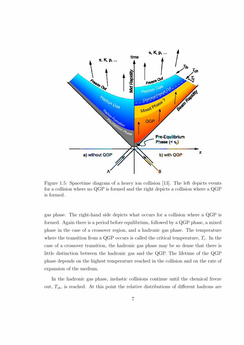
Figure 1.5: Spacetime diagram of a heavy ion collision [13]. The left depicts eventsfor a collision where no QGP is formed and the right depicts a collision where a QGPis formed.

gas phase. The right-hand side depicts what occurs for a collision where a QGP is

formed. Again there is a period before equilibrium, followed by a QGP phase, a mixed

phase in the case of a crossover region, and a hadronic gas phase. The temperature

where the transition from a QGP occurs is called the critical temperature, Tc. In the

case of a crossover transition, the hadronic gas phase may be so dense that there is

little distinction between the hadronic gas and the QGP. The lifetime of the QGP

phase depends on the highest temperature reached in the collision and on the rate of

expansion of the medium.

In the hadronic gas phase, inelastic collisions continue until the chemical freeze

out, Tch, is reached. At this point the relative distributions of different hadrons are

7

fixed. The hadrons are not necessarily in complete chemical equilibrium at this point.

Elastic collisions continue until the thermal freeze out, Tfo. At this point the momenta

of the hadrons are fixed.

1.4 Theoretical frameworks to describe heavy ion

ccollisions

Many different theoretical frameworks have been used to describe heavy ion collisions.

This is not a comprehensive review and emphasis is deliberately on theories and

models which have been connected to the results presented in this thesis. Only broad

descriptions of a QGP are discussed here; theories directly related to the results will

be discussed in Chapter 7.

There are two different classes of theoretical frameworks, those which attempt

to describe the QGP describing the interactions between quarks and gluons from

first principles and those which make assumptions about the QGP and are a more

phenomenological description of the data. Theories which attempt to describe the

interactions of quarks and gluons from first principles, such as energy loss models and

the Color Glass Condensate, are more solidly founded in QCD, however, assumptions

about the initial state and hadronization are made to relate these theories to data.

Statistical models and hydrodynamical models are dependent on assumptions about

the medium created. These classes of models both depend on the medium reaching

equilibrium, at least locally.

1.4.1 Jet quenching models

The ratio of hadron spectra in A+A collisions to that in p+ p collisions is a measure

of the degree to which hadron spectra and yields are modified in heavy ion collisions.

This ratio is divided by the number of binary collisions in an A+ A collision to give

RAA =d2NAA/dpTdη

TAAd2σpp/dpTdη. (1.1)

8

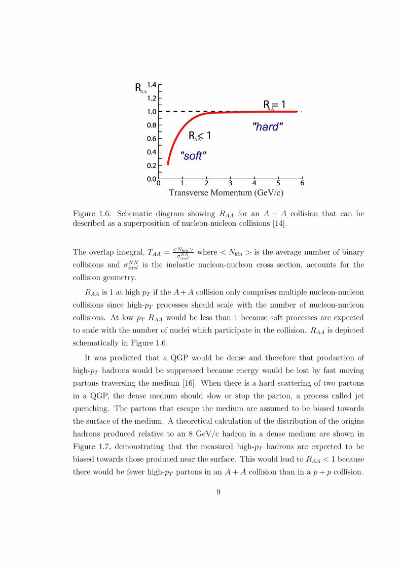
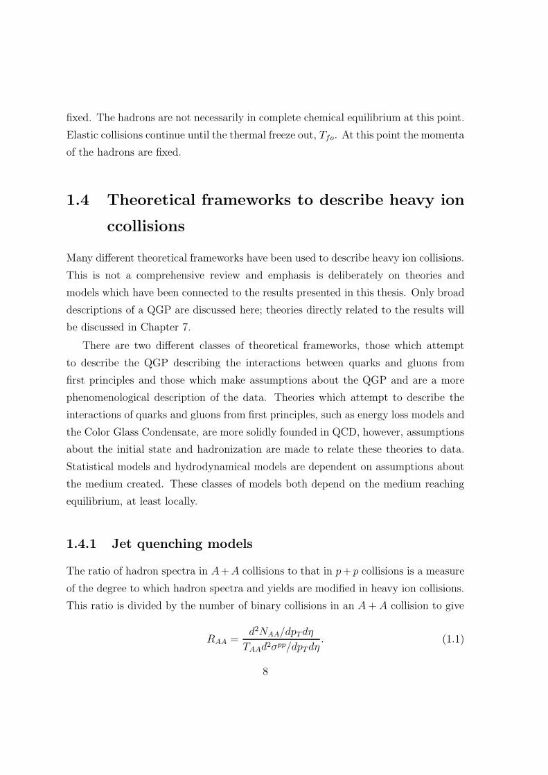
Figure 1.6: Schematic diagram showing RAA for an A + A collision that can bedescribed as a superposition of nucleon-nucleon collisions [14].

The overlap integral, TAA = <Nbin>σNN

inel

where < Nbin > is the average number of binary

collisions and σNNinel is the inelastic nucleon-nucleon cross section, accounts for the

collision geometry.

RAA is 1 at high pT if the A+A collision only comprises multiple nucleon-nucleon

collisions since high-pT processes should scale with the number of nucleon-nucleon

collisions. At low pT RAA would be less than 1 because soft processes are expected

to scale with the number of nuclei which participate in the collision. RAA is depicted

schematically in Figure 1.6.

It was predicted that a QGP would be dense and therefore that production of

high-pT hadrons would be suppressed because energy would be lost by fast moving

partons traversing the medium [16]. When there is a hard scattering of two partons

in a QGP, the dense medium should slow or stop the parton, a process called jet

quenching. The partons that escape the medium are assumed to be biased towards

the surface of the medium. A theoretical calculation of the distribution of the origins

hadrons produced relative to an 8 GeV/c hadron in a dense medium are shown in

Figure 1.7, demonstrating that the measured high-pT hadrons are expected to be

biased towards those produced near the surface. This would lead to RAA < 1 because

there would be fewer high-pT partons in an A+ A collision than in a p+ p collision.

9

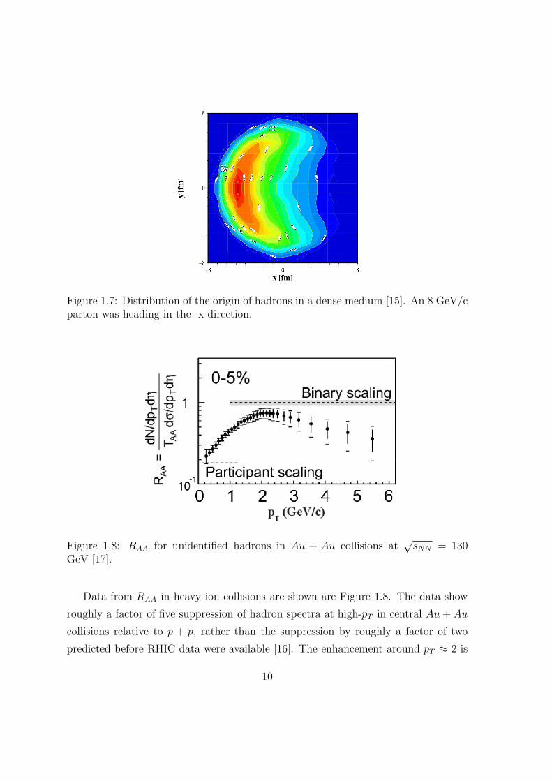
Figure 1.7: Distribution of the origin of hadrons in a dense medium [15]. An 8 GeV/cparton was heading in the -x direction.

Figure 1.8: RAA for unidentified hadrons in Au + Au collisions at√sNN = 130

GeV [17].

Data from RAA in heavy ion collisions are shown are Figure 1.8. The data show

roughly a factor of five suppression of hadron spectra at high-pT in central Au+ Au

collisions relative to p + p, rather than the suppression by roughly a factor of two

predicted before RHIC data were available [16]. The enhancement around pT ≈ 2 is

10

from the Cronin effect, first observed in d + Au collisions by J. Cronin in 1975 [18]

and has also been observed in d+Au collisions at RHIC [19]. It is believed to result

from multiple scattering of initial state partons.

Other models are capable of producing higher suppression but they require larger

partonic energy loss. Energy loss in these models is often parameterized by the

average transverse momentum lost by the parton squared per unit length, q. Attempts

have been made to determine the size of q from experimental data [20]. However,

the theoretical uncertainties are still large and estimates for q range from 0.5 - 20

GeV2/fm [21–23]. While most models can describe the suppression of light hadrons

(π, K, p) and even hadrons containing strange quarks (Λ, Λ, K0S) with a sufficiently

high q, most have trouble describing the RAA of light (u,d,s) and heavy (c,b) quarks

simultaneously [24].

1.4.2 The Glasma and the Color Glass Condensate

2

x1010 1010

Q = 200 GeV

Q = 20 GeV

xG(x,Q )

2 2

2 2

-4 -3 -2 -1

= 5 GeV2Q

2

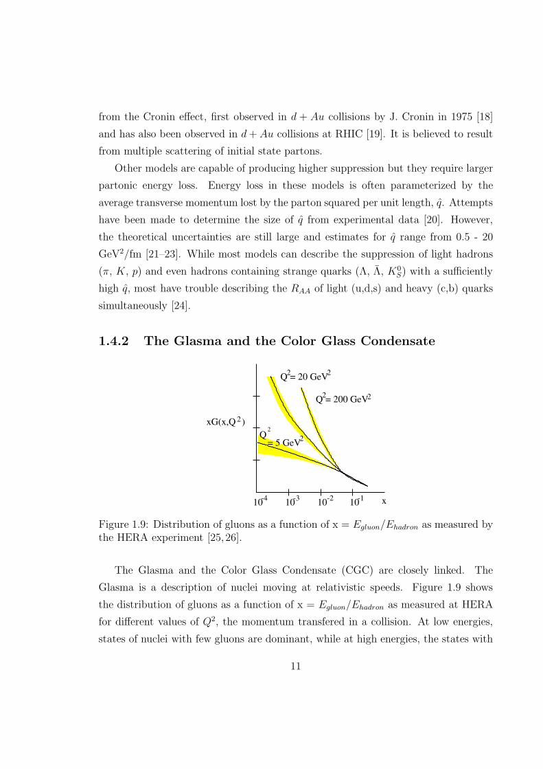
Figure 1.9: Distribution of gluons as a function of x = Egluon/Ehadron as measured bythe HERA experiment [25, 26].

The Glasma and the Color Glass Condensate (CGC) are closely linked. The

Glasma is a description of nuclei moving at relativistic speeds. Figure 1.9 shows

the distribution of gluons as a function of x = Egluon/Ehadron as measured at HERA

for different values of Q2, the momentum transfered in a collision. At low energies,

states of nuclei with few gluons are dominant, while at high energies, the states with

11

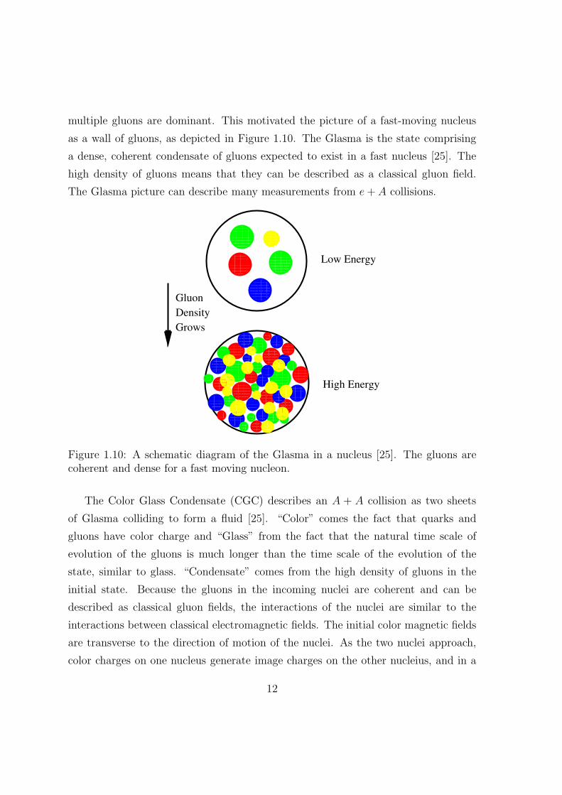
multiple gluons are dominant. This motivated the picture of a fast-moving nucleus

as a wall of gluons, as depicted in Figure 1.10. The Glasma is the state comprising

a dense, coherent condensate of gluons expected to exist in a fast nucleus [25]. The

high density of gluons means that they can be described as a classical gluon field.

The Glasma picture can describe many measurements from e+ A collisions.

Low Energy

High Energy

Gluon

Density

Grows

Figure 1.10: A schematic diagram of the Glasma in a nucleus [25]. The gluons arecoherent and dense for a fast moving nucleon.

The Color Glass Condensate (CGC) describes an A + A collision as two sheets

of Glasma colliding to form a fluid [25]. “Color” comes the fact that quarks and

gluons have color charge and “Glass” from the fact that the natural time scale of

evolution of the gluons is much longer than the time scale of the evolution of the

state, similar to glass. “Condensate” comes from the high density of gluons in the

initial state. Because the gluons in the incoming nuclei are coherent and can be

described as classical gluon fields, the interactions of the nuclei are similar to the

interactions between classical electromagnetic fields. The initial color magnetic fields

are transverse to the direction of motion of the nuclei. As the two nuclei approach,

color charges on one nucleus generate image charges on the other nucleius, and in a

12

short period of time the direction of the fields changes from transverse to parallel to

the direction of the movement nuclei. The medium produced from the interaction of

quarks and gluons in these fields is the CGC [25].

1.4.3 Statistical models

Hadronization of quarks and gluons is not calculable from QCD first principles. Statis-

tical models are one of the models describing the hadronization of quarks and gluons.

The first statistical models for hadronization were proposed before the development

of QCD and interest was renewed when it was proposed that an equilibrated hadron

gas might be a signature for a QGP [27]. These models calculated particle ratios in

a hadron gas at chemical equilibrium and deal with the conserved quantities: baryon

number (B), strangeness (S), and charge (C). Calculations for elementary collisions

such as e+ + e−, p + p, and p + p must use a canonical ensemble to describe hadron

production. In heavy ion collisions the volume of the system is large enough that it

can be described by a grand canonical ensemble and the conserved quantities have

corresponding chemical potentials [28]. The log of the partition function in the grand

canonical ensemble is given by

ln(Z) =∑

speciesi

giV

(2π)3

∫

ln(1 ± e−β(Ei−µi)±1d3p (1.2)

where gi is the degeneracy of the state, V is the volume of the system, β = 1kT

, k is

the Boltzman constant, T is the temperature, Ei =√

p2 +m2i is the particle energy,

mi is the particle mass, p is the particle momentum, and µi is the particle’s chemical

potential. The µi are given by

µi = BiµB + SiµS +QiµQ (1.3)

where µB is the baryon chemical potential, µS is the strangeness chemical potential,

and µQ is the chemical potential corresponding to charge. The number of particles of

each species is given by

Ni = T∂lnZ

∂µi=giV

2π2

∞∑

k=1

m2iT

kK2(

kmi

T)eβkµi (1.4)

13

Figure 1.11: Thermal fit to RHIC data on yields of hadrons [29]. γs is a factorindicating the degree of equilibration of strange quarks. γs = 1 indicates completeequilibration.

where K2 is the modified Bessel function.

Since the volume of the medium produced in a heavy ion collision cannot be

measured directly, statistical models cannot be used to calculate the absolute yields,

however, they can be used to calculate the relative yields of particles. Statistical

models do not describe strangeness well so an ad hoc parameter γs was introduced to

account for the suppression of hadrons with strange valence quarks relative to their

equilibrium value. γs = 1 if strangeness is in equilibrium. Measured particle ratios

are fit to determine µB, µS, µQ, γs and T. Further details of these calculations can

be found in [27] and the references therein.

Figure 1.11 shows a fit of a statistical model described in [30] to particle ratios

in Au + Au collisions at√sNN = 200 GeV, demonstrating that statistical models

describe the data well. The inset shows γs as a function of the number of participants

in the collisions, with collision centrality increasing with the number of participants.

γs ≈ 1 for central collisions.

If the medium does reach equilibrium, statistical models must describe the data,

14

however, this is not a sufficient condition to prove that the medium has reached

equilibrium. Statistical models also describe e+ + e−, p + p, and p + p collisions

reasonably well with γs in the range of 0.4-0.8 [27]. The interpretation of this fact has

been much debated. It is possible that the hadrons are produced in equilibrium, but it

means that statistical models alone cannot be interpreted as proof of an equilibrated

medium.

Regardless of the collision system, the temperature attained from thermal fits is

remarkably constant at around 160 MeV, with the fits of STAR data in Figure 1.11

giving T = 163 ± 4 MeV [29]. This should not be interpreted as the temperature of

the QGP, but rather as the chemical freeze out temperature Tch. Statistical models

cannot describe the full spectra of hadrons produced in a heavy ion collision but

rather are limited to describing the overall yield of particles.

1.4.4 Hydrodynamics

Hydrodynamical models describe the medium as a relativistic fluid. Several of these

models describe a fluid with a viscosity of zero [31–34]. These models are not restricted

to describing a QGP but rather can describe any relativistic fluid.

Hydrodynamical observables are related to two major features in heavy ion col-

lisions. First, the region where the incoming nuclei overlap is asymmetric and this

spatial anisotropy in the initial state results in a momentum anisotropy in the final

state. This phenomenon is called anisotropic flow. Second, the large pressure gradi-

ents lead the medium to expand and particles to move away from the collision point.

This phenomenon is called radial flow.

Figure 1.12 shows the geometric relationship between the reaction plane and the

incoming nuclei. The overlap region between the two incoming nuclei is almond

shaped, and the reaction plane is the plane formed by the beam axis and the centers

of both nuclei. For a large impact parameter, the distance between the centers of the

the two nuclei, the overlap region is more oblong while for a smaller impact parameter

the overlap region is closer to circular.

15

Figure 1.12: Diagram showing the location of the reaction plane relative to the in-coming nuclei [13].

−10 −5 0 5 10

−10

−5

0

5

10

x (fm)

y (

fm)

Figure 1.13: Contours of constant density in a hydrodynamical model [35]. Theprojections of the incoming nuclei are shown as dashed lines. The impact parameteris 7 fm.

It is assumed that the azimuthal momentum anisotropy originates from the collec-

tive movement of a fluid formed at early stages of the collision. This is the most uni-

versally accepted mechanism for the production of an azimuthal anisotropy, however,

other mechanisms have been proposed [36–39]. In a hydrodynamical model, the initial

16

anisotropy in the distribution of particles leads to a pressure gradient. Figure 1.13

shows theoretical calculations for the contours of constant density. The pressure gra-

dient is perpendicular to these lines, meaning that it is azimuthally anisotropic. As

the system evolves, the spatial azimuthal anisotropy in the distribution of particles

will disappear. The anisotropy in the momentum distribution of particles due to the

pressure gradient will remain.

The initial azimuthal anisotropy is often described in terms of the Fourier expan-

sion of the distribution of particles in momentum:

Ed3N

d3pT=

1

2π

d2N

pTdpTdy(1 +

∞∑

n=1

2vncos(n(φ− ψRP ))). (1.5)

v1 is called directed flow and describes the preference for particles to move in the

direction along the beam axis. v2 is called elliptic flow and describes the tendency

for particles to have a preferred direction of motion in the x-y plane as a result of

the spatial anisotropy in the initial condition [40]. Experimentally, the vn are small

and decreasing with increasing n in heavy ion collisions. v2 has been studied most

extensively.

Figure 1.14 shows the magnitude of v2 in A + A collisions as a function of the

energy per nucleon in the collision. At very low energies, the nucleons simply scatter

off each other (bounce-off), leading to a positive v2. At intermediate collision energies,

particles created in the collision cannot move in the direction of the short axis of the

overlap region because they would collide with the constituent nucleons of the colliding

nuclei, bouncing them back in towards the overlap region. The only direction where

particles could escape is in the direction of the long axis of the overlap region since

there is no matter there to stop particles from escaping, leading to a negative v2

(squeeze-out).

At higher collision energies, the incoming nuclei are Lorentz contracted so that

the nucleus is effectively flat and all nucleons interact at nearly the same time. Any

nucleons which did not participate in the interaction have already moved past the

interaction region and can no longer collide with the particles created in the collision.

v2 becomes positive again.

Figure 1.15 shows measurements of v2 at various collision energies compared to

17

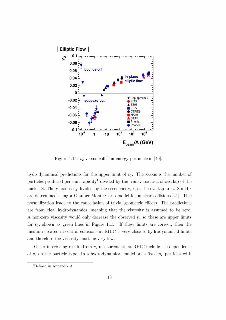
Figure 1.14: v2 versus collision energy per nucleon [40].

hydrodynamical predictions for the upper limit of v2. The x-axis is the number of

particles produced per unit rapidity1 divided by the transverse area of overlap of the

nuclei, S. The y-axis is v2 divided by the eccentricity, ǫ, of the overlap area. S and ǫ

are determined using a Glauber Monte Carlo model for nuclear collisions [41]. This

normalization leads to the cancellation of trivial geometric effects. The predictions

are from ideal hydrodynamics, meaning that the viscosity is assumed to be zero.

A non-zero viscosity would only decrease the observed v2 so these are upper limits

for v2, shown as green lines in Figure 1.15. If these limits are correct, then the

medium created in central collisions at RHIC is very close to hydrodynamical limits

and therefore the viscosity must be very low.

Other interesting results from v2 measurements at RHIC include the dependence

of v2 on the particle type. In a hydrodynamical model, at a fixed pT particles with

1Defined in Appendix A

18

Figure 1.15: v2 measurements compared to hydroynamical limits in different models[40]. The x-axis is a measure of the number of particles produced per unit of rapidityat mid-rapidity divided by the transverse overlap area in the collision. The y-axisis v2 divided by the eccentricity of the overlap area. The green arrow indicates thepredicted position of a color percolation phase transition. The green lines indicatethe ideal hydrodynamics predictions for AGS, SPS, and RHIC energies.

Figure 1.16: Particle species dependence of v2 at low-pT [40].

19

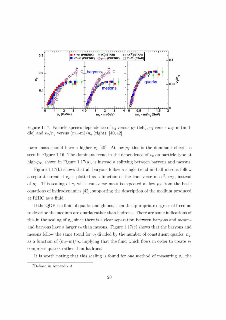
Figure 1.17: Particle species dependence of v2 versus pT (left), v2 versus mT -m (mid-dle) and v2/nq versus (mT -m)/nq (right). [40, 42].

lower mass should have a higher v2 [40]. At low-pT this is the dominant effect, as

seen in Figure 1.16. The dominant trend in the dependence of v2 on particle type at

high-pT , shown in Figure 1.17(a), is instead a splitting between baryons and mesons.

Figure 1.17(b) shows that all baryons follow a single trend and all mesons follow

a separate trend if v2 is plotted as a function of the transverse mass2, mT , instead

of pT . This scaling of v2 with transverse mass is expected at low pT from the basic

equations of hydrodynamics [42], supporting the description of the medium produced

at RHIC as a fluid.

If the QGP is a fluid of quarks and gluons, then the appropriate degrees of freedom

to describe the medium are quarks rather than hadrons. There are some indications of

this in the scaling of v2, since there is a clear separation between baryons and mesons

and baryons have a larger v2 than mesons. Figure 1.17(c) shows that the baryons and

mesons follow the same trend for v2 divided by the number of constituent quarks, nq,

as a function of (mT -m)/nq implying that the fluid which flows in order to create v2

comprises quarks rather than hadrons.

It is worth noting that this scaling is found for one method of measuring v2, the

2Defined in Appendix A

20

0 10 20 30 40 50 60 70 80 (

%)

2v

0

2

4

6

8

Event Plane

4 Cumu.

LYZ_Sum

LYZ_Prod

(a)

% Most Central0 10 20 30 40 50 60 70 80

EP

2

/v2

v

0.7

0.8

0.9

1

1.1 (b)

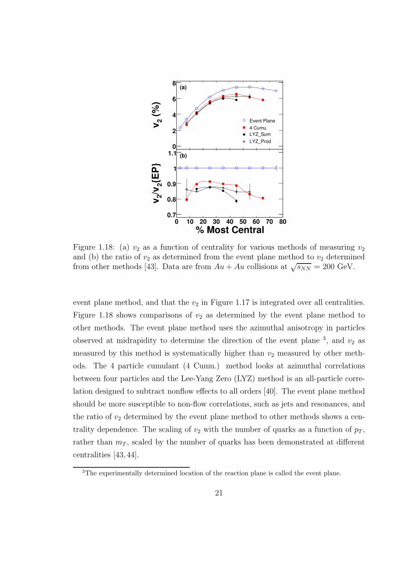
Figure 1.18: (a) v2 as a function of centrality for various methods of measuring v2

and (b) the ratio of v2 as determined from the event plane method to v2 determinedfrom other methods [43]. Data are from Au+ Au collisions at

√sNN = 200 GeV.

event plane method, and that the v2 in Figure 1.17 is integrated over all centralities.

Figure 1.18 shows comparisons of v2 as determined by the event plane method to

other methods. The event plane method uses the azimuthal anisotropy in particles

observed at midrapidity to determine the direction of the event plane 3, and v2 as

measured by this method is systematically higher than v2 measured by other meth-

ods. The 4 particle cumulant (4 Cumu.) method looks at azimuthal correlations

between four particles and the Lee-Yang Zero (LYZ) method is an all-particle corre-

lation designed to subtract nonflow effects to all orders [40]. The event plane method

should be more susceptible to non-flow correlations, such as jets and resonances, and

the ratio of v2 determined by the event plane method to other methods shows a cen-

trality dependence. The scaling of v2 with the number of quarks as a function of pT ,

rather than mT , scaled by the number of quarks has been demonstrated at different

centralities [43, 44].

3The experimentally determined location of the reaction plane is called the event plane.

21

Since hydrodynamics assumes thermalization, the success of ideal hydrodynamics

at describing many aspects of RHIC data implies that the medium is thermalized when

v2 is formed. Figure 1.17 demonstrates that hadrons containing strange quarks follow

the same trends for v2, implying that strangeness is also thermalized. Furthermore,

not only is strangeness thermalized, but measurements of electrons from decays of

hadrons including charm quarks indicate that the v2 of charm quarks is probably

comparable to that of light quarks [24].

Radial flow is also predicted by hydrodynamics. The medium is expanding because

of pressure gradients, as depicted in Figure 1.13. This means that on average particles

are moving away from the center of the interaction region. Both radial flow and

anisotropic flow alter the spectra of particles, since both affect the momentum of

particles. Radial flow is expected to have a mass dependence, similar to anisotropic

flow. Fits of data to a hydrodynamical model inspired parameterization of spectra

called a Blast Wave Model give values for radial flow consistent with those expected

from hydrodynamics. These models yield anisotropic flow comparable to independent

measurements [40].

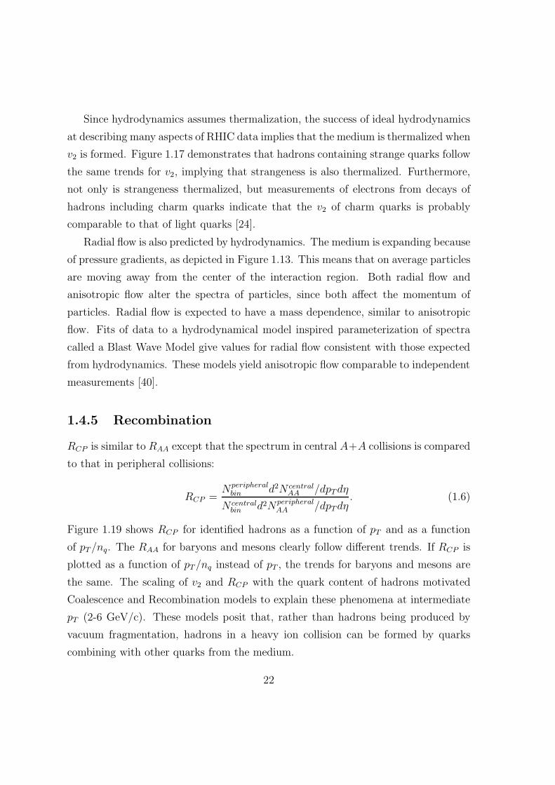
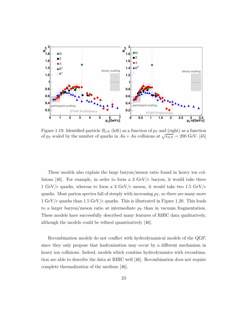
1.4.5 Recombination

RCP is similar to RAA except that the spectrum in central A+A collisions is compared

to that in peripheral collisions:

RCP =Nperipheral

bin d2N centralAA /dpTdη

N centralbin d2Nperipheral

AA /dpTdη. (1.6)

Figure 1.19 shows RCP for identified hadrons as a function of pT and as a function

of pT /nq. The RAA for baryons and mesons clearly follow different trends. If RCP is

plotted as a function of pT /nq instead of pT , the trends for baryons and mesons are

the same. The scaling of v2 and RCP with the quark content of hadrons motivated

Coalescence and Recombination models to explain these phenomena at intermediate

pT (2-6 GeV/c). These models posit that, rather than hadrons being produced by

vacuum fragmentation, hadrons in a heavy ion collision can be formed by quarks

combining with other quarks from the medium.

22

0 1 2 3 4 5 6 7

0.2

0.4

0.6

0.8

1

1.2

1.4

1.6

1.8

2

STAR Preliminary

participant scaling

binary scaling

Ω

Ξ

Λ

0K±K

[GeV/c]T

p

CP

R

0 0.5 1 1.5 2 2.5 3 3.5

0.2

0.4

0.6

0.8

1

1.2

1.4

1.6

1.8

2

STAR Preliminary

participant scaling

binary scaling

Ω

Ξ

Λ

0K

/n[GeV/c]T

p

CP

R

Figure 1.19: Identified particle RCP (left) as a function of pT and (right) as a functionof pT scaled by the number of quarks in Au+Au collisions at

√sNN = 200 GeV. [45]

These models also explain the large baryon/meson ratio found in heavy ion col-

lisions [46]. For example, in order to form a 3 GeV/c baryon, it would take three

1 GeV/c quarks, whereas to form a 3 GeV/c meson, it would take two 1.5 GeV/c

quarks. Most parton spectra fall of steeply with increasing pT , so there are many more

1 GeV/c quarks than 1.5 GeV/c quarks. This is illustrated in Figure 1.20. This leads

to a larger baryon/meson ratio at intermediate pT than in vacuum fragmentation.

These models have successfully described many features of RHIC data qualitatively,

although the models could be refined quantitatively [46].

Recombination models do not conflict with hydrodynamical models of the QGP,

since they only propose that hadronization may occur by a different mechanism in

heavy ion collisions. Indeed, models which combine hydrodynamics with recombina-

tion are able to describe the data at RHIC well [46]. Recombination does not require

complete thermalization of the medium [46].

23

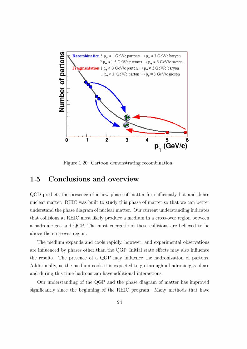
Figure 1.20: Cartoon demonstrating recombination.

1.5 Conclusions and overview

QCD predicts the presence of a new phase of matter for sufficiently hot and dense

nuclear matter. RHIC was built to study this phase of matter so that we can better

understand the phase diagram of nuclear matter. Our current understanding indicates

that collisions at RHIC most likely produce a medium in a cross-over region between

a hadronic gas and QGP. The most energetic of these collisions are believed to be

above the crossover region.

The medium expands and cools rapidly, however, and experimental observations

are influenced by phases other than the QGP. Initial state effects may also influence

the results. The presence of a QGP may influence the hadronization of partons.

Additionally, as the medium cools it is expected to go through a hadronic gas phase

and during this time hadrons can have additional interactions.

Our understanding of the QGP and the phase diagram of matter has improved

significantly since the beginning of the RHIC program. Many methods that have

24

been used to describe a QGP qualitatively describe the features of the data, however,

we do not yet have a complete quantitative description of the data. Some meth-

ods attempt to make predictions by calculating results directly from QCD. Provided

that the approximations are valid, these theories should describe the partonic phases

well, however, they are dependent on models of hadronization and interactions in a

hadronic gas phase. Our knowledge of hadronization is heavily dependent upon ex-

perimental data because hadronization is a non-perturbative process. If the medium

goes through a hadronic gas phase for any significant amount of time and hadrons re-

interact, this would also change the properties of measured hadrons. Either of these

effects or invalid assumptions made in calculations could be responsible for deviations

between QCD-based theories and experimental data.

Many phenomenological models have been successfully used to describe the ex-

perimental data. Hydrodynamics in particular has been useful to describe not only

azimuthal anisotropies but also hadron spectra. The success of hydro at describing

many features of the data implies that the medium produced is a fluid made up

of partons instead of hadrons. Hydrodynamics, however, is heavily dependent on

thermalization of the medium and there is no conclusive proof that the medium has

reached thermal equilibrium. Statistical models are consistent with the data but the

agreement with these models is not sufficient to prove that the medium has reached

thermal equilibrium. Recombination models have successfully described many aspects

of the data and also point towards a picture of a medium characterized by partonic

rather than hadronic degrees of freedom. Recombination models, which posit a mod-

ified hadronization mechanism in heavy ion collisions, are not dependent on complete

thermalization and are consistent with hydrodynamical models.

These models and theories are not all mutually exclusive and may be valid in

different regimes. The best way to test these models is compare them to as many

measurements as possible. The studies presented in this thesis will focus on studies

of jets formed by partons which have traversed the medium, taking advantage of

the wealth of data available at RHIC. Jet-like di-hadron correlations are studied as

a function of the collision system (Cu + Cu versus Au + Au), the collision energy

(√sNN = 62 GeV versus

√sNN = 200 GeV), and particle type and strangeness content

25

(unidentified hadrons, Λ, K0S, and Ξ).

Chapter 2 will introduce high-pT triggered di-hadron correlations and discuss other

relevant studies, performed either previously or concurrently. Here the two promi-

nent features in di-hadron correlations, the jet-like correlation and the Ridge, will be

introduced. These features are from particles close in azimuth to the trigger particle,

called the near-side of the correlation. The properties learned from studies of the

near-side in Au + Au collisions at√sNN = 200 GeV will be discussed. This will

be followed by an overview of the experiment in Chapter 3. The analysis methods

will be presented in Chapter 4 and Chapter 5, first discussing how particles used in

the analysis are selected and then discussing the method for measuring di-hadron

correlations. The results for the system, energy, and particle type dependence will be

discussed in Chapter 6 and their interpretation in light of other data and of models

will be discussed in Chapter 7. Chapter 8 will conclude and discuss the outlook for

future studies of jets in heavy ion collisions. Di-hadron correlations after background

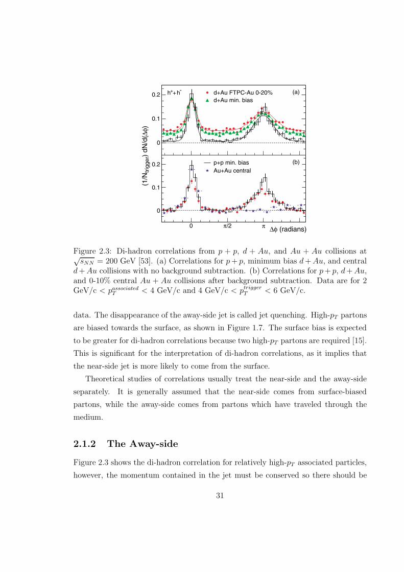
subtraction

26

Chapter 2

Jets as a probe of a Quark-Gluon

Plasma

Due to confinement, particles which carry a color charge, such as quarks and gluons,

cannot be directly observed. Instead, they fragment into hadrons, which are color-

neutral, and these hadrons are detected. In hard scattering processes the majority of

the hadrons are produced roughly colinear to the fragmenting partons, resulting in

a narrow cone of hadrons called a jet. At RHIC energies most jets are produced in

2→2 scattering of hard partons from the incoming nuclei. Since the incoming partons

have momenta nearly parallel with the nuclei, momentum conservation causes the

scattered partons to be separated by roughly 180° in azimuth. Events with jets at

RHIC energies are dominantly back-to-back di-jets. Figure 2.1 shows an example of

a di-jet event in STAR. The beam goes through the center and the lines show the

different sectors of the Time Projection Chamber.

The jet cross section can be calculated in perturbative QCD as the average of

quark, anti-quark, and gluon processes. For two partons scattering the jet cross

section is given by

σi,j→k =∑

i,j

∫

dx1dx2dtf1i (x1, Q

2)f 2j (x2, Q

2)dσi,j→k

dt(2.1)

where x1 and x2 are the fraction of the nucleon’s momentum carried by the parton,

Q2 is the momentum transfer in the scattering, f 1i and f 2

j are the parton distribution

27

Figure 2.1: Sample jet observed in STAR in a real p + p collision at√sNN = 200

GeV

functions in the nucleons, and σi,j→k is the cross section for the reaction ij → k [47].

Parton distribution functions are the probability densities for finding a parton as a

function of Q2 and x.

After the hard scattering, the scattered partons hadronize. The process of hadroniza-

tion is non-perturbative. It is described by fragmentation functions, which represent

the probability for a parton to fragment into a particular hadron. Fragmentation

functions have not been determined from first principles, however, it is possible to

parameterize them as functions of the parton energy and the fraction of energy carried

by the parton and then determine the fragmentation functions from data. Vacuum

fragmentation functions have been well constrained by data from elementary colli-

sions.

In heavy ion collisions, jets are formed from parton scattering which likely occurs

early in the collision. The partons then travel through the medium and therefore serve

as a probe of the medium. This scenario is depicted in Figure 2.2. Since jets have been

studied extensively in p+p collisions, modifications of jets in A+A collisions relative

to p+p can be attributed to interactions with the medium. These modifications may

28

Figure 2.2: Schematic diagram of a di-jet in a heavy ion collision. The red arrowdenotes the leading hadron, the one with the highest pT , and the black arrows denoteother hadrons produced during hadronization.

come in the form of parton energy loss before fragmentation or modification of the

fragmentation functions for partons that fragment in the medium.

There have been many different approaches to studying jets at RHIC. In this

chapter the various methods and key results from RHIC are reviewed. Some of these

studies occurred concurrently with the analyses presented in this thesis, and discussion

of these results is necessary to form a complete picture of what can be learned from

the data on jets at RHIC.

2.1 Studies of jets through high-pT triggered di-

hadron correlations

In di-hadron correlations, a high momentum particle is selected and the distribution

of particles relative to that particle is determined. The former particle is called the

trigger particle and the latter are called the associated particles. The primary criterion

used to determine trigger and associated particles is their momenta and the method

29

neglects contributions from any sources of correlations between high-pT particles other

than jets and anisotropic flow. Anisotropic flow is a background and its subtraction is

discussed further in Chapter 5. The momenta of the trigger and associated particles

are restricted to high-pT to increase the probability that the particles come from

a jet and therefore decrease the combinatorial background. It has been argued that

contributions from other sources are non-negligible. In particular it has been proposed

that a significant fraction of trigger particles may not come from jets [48]. The STAR

collaboration presented correlations normalized per trigger particle and with this

normalization, results from different systems (p+ p, d+Au, Cu+Cu, and Au+Au)

would be identical if there were no modification of the jet [49–55]. The PHENIX

collaboration typically used a different normalization where the amplitude of the

correlation is interpreted as the probability for an associated particle to be correlated

with the jet [56–62].

2.1.1 Early studies of jets at RHIC

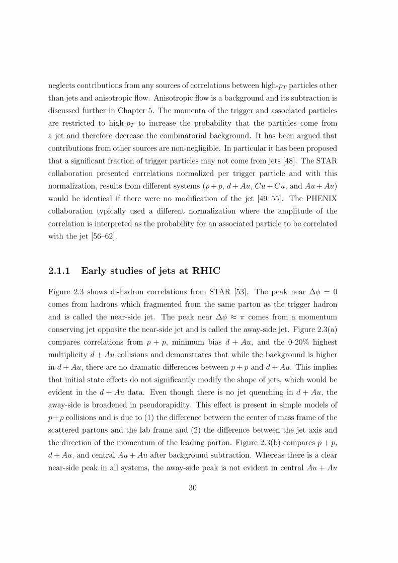
Figure 2.3 shows di-hadron correlations from STAR [53]. The peak near ∆φ = 0

comes from hadrons which fragmented from the same parton as the trigger hadron

and is called the near-side jet. The peak near ∆φ ≈ π comes from a momentum

conserving jet opposite the near-side jet and is called the away-side jet. Figure 2.3(a)

compares correlations from p + p, minimum bias d + Au, and the 0-20% highest

multiplicity d + Au collisions and demonstrates that while the background is higher

in d+Au, there are no dramatic differences between p+ p and d+Au. This implies

that initial state effects do not significantly modify the shape of jets, which would be

evident in the d + Au data. Even though there is no jet quenching in d + Au, the

away-side is broadened in pseudorapidity. This effect is present in simple models of

p+p collisions and is due to (1) the difference between the center of mass frame of the

scattered partons and the lab frame and (2) the difference between the jet axis and

the direction of the momentum of the leading parton. Figure 2.3(b) compares p+ p,

d+Au, and central Au+Au after background subtraction. Whereas there is a clear

near-side peak in all systems, the away-side peak is not evident in central Au + Au

30

0

0.1

0.2 d+Au FTPC-Au 0-20%

d+Au min. bias

0

0.1

0.2 p+p min. bias

Au+Au central

(1/N

trig

ge

r) d

N/d

(∆φ

)

∆φ (radians)0 π /2 π

(a)

(b)

h++h-

Figure 2.3: Di-hadron correlations from p + p, d + Au, and Au + Au collisions at√sNN = 200 GeV [53]. (a) Correlations for p+ p, minimum bias d+Au, and central

d+Au collisions with no background subtraction. (b) Correlations for p+ p, d+Au,and 0-10% central Au + Au collisions after background subtraction. Data are for 2GeV/c < passociated

T < 4 GeV/c and 4 GeV/c < ptriggerT < 6 GeV/c.

data. The disappearance of the away-side jet is called jet quenching. High-pT partons

are biased towards the surface, as shown in Figure 1.7. The surface bias is expected

to be greater for di-hadron correlations because two high-pT partons are required [15].

This is significant for the interpretation of di-hadron correlations, as it implies that

the near-side jet is more likely to come from the surface.

Theoretical studies of correlations usually treat the near-side and the away-side

separately. It is generally assumed that the near-side comes from surface-biased

partons, while the away-side comes from partons which have traveled through the

medium.

2.1.2 The Away-side

Figure 2.3 shows the di-hadron correlation for relatively high-pT associated particles,

however, the momentum contained in the jet must be conserved so there should be

31

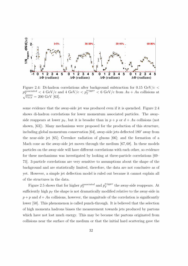
Figure 2.4: Di-hadron correlations after background subtraction for 0.15 GeV/c <passociated

T < 4 GeV/c and 4 GeV/c < ptriggerT < 6 GeV/c from Au + Au collisions at√

sNN = 200 GeV [63].

some evidence that the away-side jet was produced even if it is quenched. Figure 2.4

shows di-hadron correlations for lower momentum associated particles. The away-

side reappears at lower pT , but it is broader than in p + p or d + Au collisions (not

shown, [63]). Many mechanisms were proposed for the production of this structure,

including global momentum conservation [64], away-side jets deflected 180° away from

the near-side jet [65]; Cerenkov radiation of gluons [66]; and the formation of a

Mach cone as the away-side jet moves through the medium [67,68]. In these models

particles on the away-side will have different correlations with each other, so evidence

for these mechanisms was investigated by looking at three-particle correlations [69–

73]. 3-particle correlations are very sensitive to assumptions about the shape of the

background and are statistically limited, therefore, the data are not conclusive as of

yet. However, a simple jet deflection model is ruled out because it cannot explain all

of the structures in the data.

Figure 2.5 shows that for higher passociatedT and ptrigger

T the away-side reappears. At

sufficiently high pT the shape is not dramatically modified relative to the away-side in

p+ p and d+Au collisions, however, the magnitude of the correlation is significantly

lower [50]. This phenomenon is called punch-through. It is believed that the selection

of high momenta hadrons biases the measurement towards jets produced by partons

which have not lost much energy. This may be because the partons originated from

collisions near the surface of the medium or that the initial hard scattering gave the

32

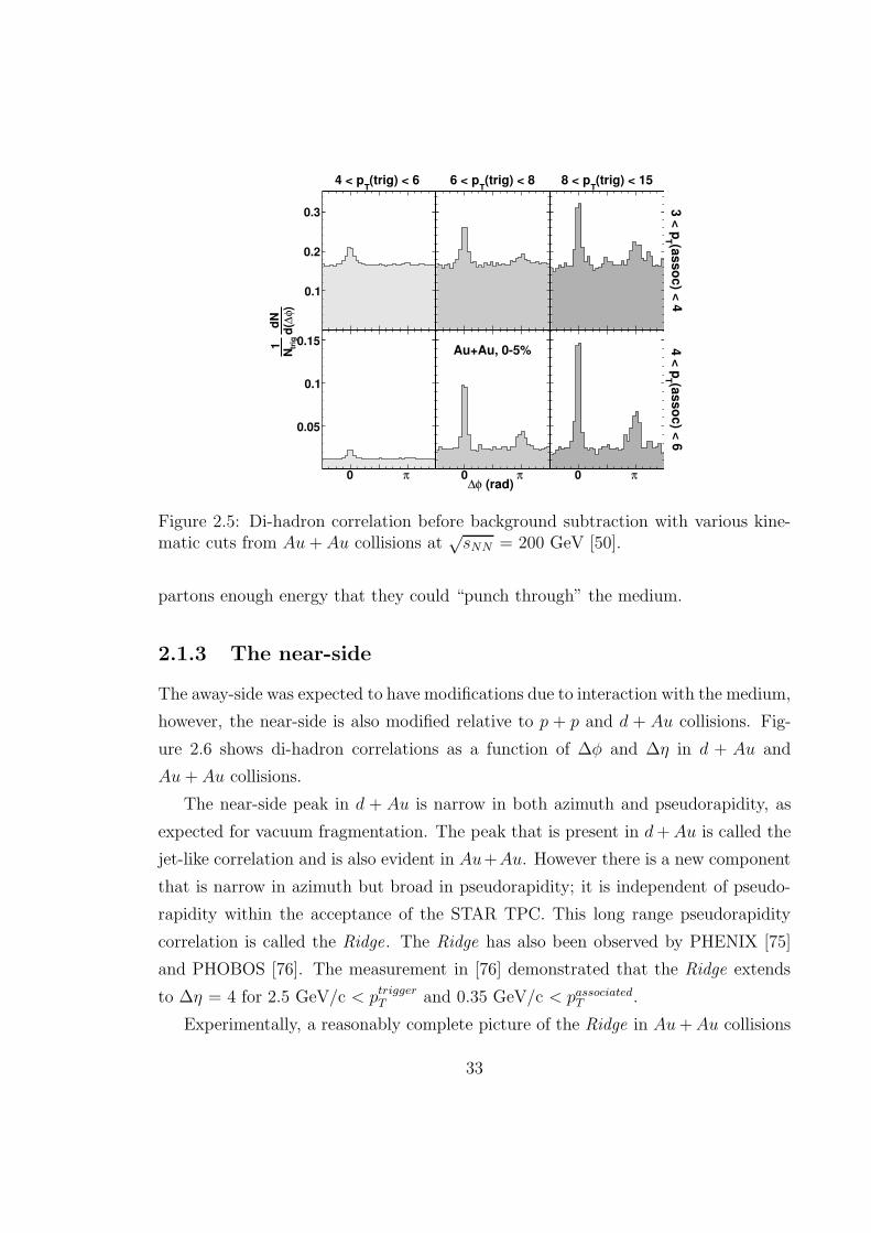
Au+Au, 0-5%

0.1

0.2

0.3

0.05

0.1

0.15

(asso

c) <

4T

3 <

p(a

sso

c) <

6T

4 <

p

(rad)φ∆0 π 0 π 0 π

(trig) < 6T

4 < p (trig) < 8T

6 < p (trig) < 15T

8 < p

)φ

∆d

(dN

tr

igN

1

Figure 2.5: Di-hadron correlation before background subtraction with various kine-matic cuts from Au+ Au collisions at

√sNN = 200 GeV [50].

partons enough energy that they could “punch through” the medium.

2.1.3 The near-side

The away-side was expected to have modifications due to interaction with the medium,

however, the near-side is also modified relative to p + p and d + Au collisions. Fig-

ure 2.6 shows di-hadron correlations as a function of ∆φ and ∆η in d + Au and

Au+ Au collisions.

The near-side peak in d + Au is narrow in both azimuth and pseudorapidity, as

expected for vacuum fragmentation. The peak that is present in d+Au is called the

jet-like correlation and is also evident in Au+Au. However there is a new component

that is narrow in azimuth but broad in pseudorapidity; it is independent of pseudo-

rapidity within the acceptance of the STAR TPC. This long range pseudorapidity

correlation is called the Ridge. The Ridge has also been observed by PHENIX [75]

and PHOBOS [76]. The measurement in [76] demonstrated that the Ridge extends

to ∆η = 4 for 2.5 GeV/c < ptriggerT and 0.35 GeV/c < passociated

T .

Experimentally, a reasonably complete picture of the Ridge in Au+Au collisions

33

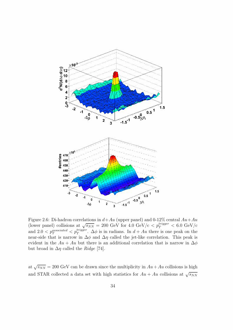
Figure 2.6: Di-hadron correlations in d+Au (upper panel) and 0-12% central Au+Au(lower panel) collisions at

√sNN = 200 GeV for 4.0 GeV/c < ptrigger

T < 6.0 GeV/c

and 2.0 < passociatedT < ptrigger

T . ∆φ is in radians. In d + Au there is one peak on thenear-side that is narrow in ∆φ and ∆η called the jet-like correlation. This peak isevident in the Au + Au but there is an additional correlation that is narrow in ∆φbut broad in ∆η called the Ridge [74].

at√sNN = 200 GeV can be drawn since the multiplicity in Au+Au collisions is high

and STAR collected a data set with high statistics for Au + Au collisions at√sNN

34

Figure 2.7: The number of particles in the Ridge and the jet-like correlation (J+R)and in the jet-like correlation alone (J) as a function of Npart for 4.0 < ptrigger

T < 6.0GeV/c and 2.0 < passociated

T < 4.0 GeV/c within -1.75 < ∆η < 1.75 for 0-12% centralAu + Au collisions at

√sNN = 200 GeV [74]. The solid lines show the systematic

error.

= 200 GeV in 2004. Figure 2.7 shows the number of particles in both the Ridge and

the jet-like correlation combined and in the jet-like correlation alone as a function

of Npart. The number of particles in the jet-like correlation is determined using two

methods: (1) by subtracting the contribution from the Ridge and (2) determining

the yield in azimuth and determining the number of particles in the peak above the

plateau in pseudorapidity. These methods are discussed futher in Chapter 5. The

jet-like correlation alone is almost independent of Npart, while the Ridge grows with

Npart. The Ridge is not present in d+ Au [77].

The jet-like yield normalized per trigger should remain constant as a function

of Npart if jet production in A + A collisions is identical to jet production in p + p

collisions. If the yield per trigger changes as a function of Npart this may indicate

that jet production is modified by the medium. Figure 2.7 indicates that the jet-like

correlation may result from processes that occur in p + p collisions while the Ridge

results from processes that either do not occur in p+ p collisions or those which are

more prominent in A + A collisions.

Figure 2.8 shows the number of particles in the Ridge as a function of ptriggerT .

35

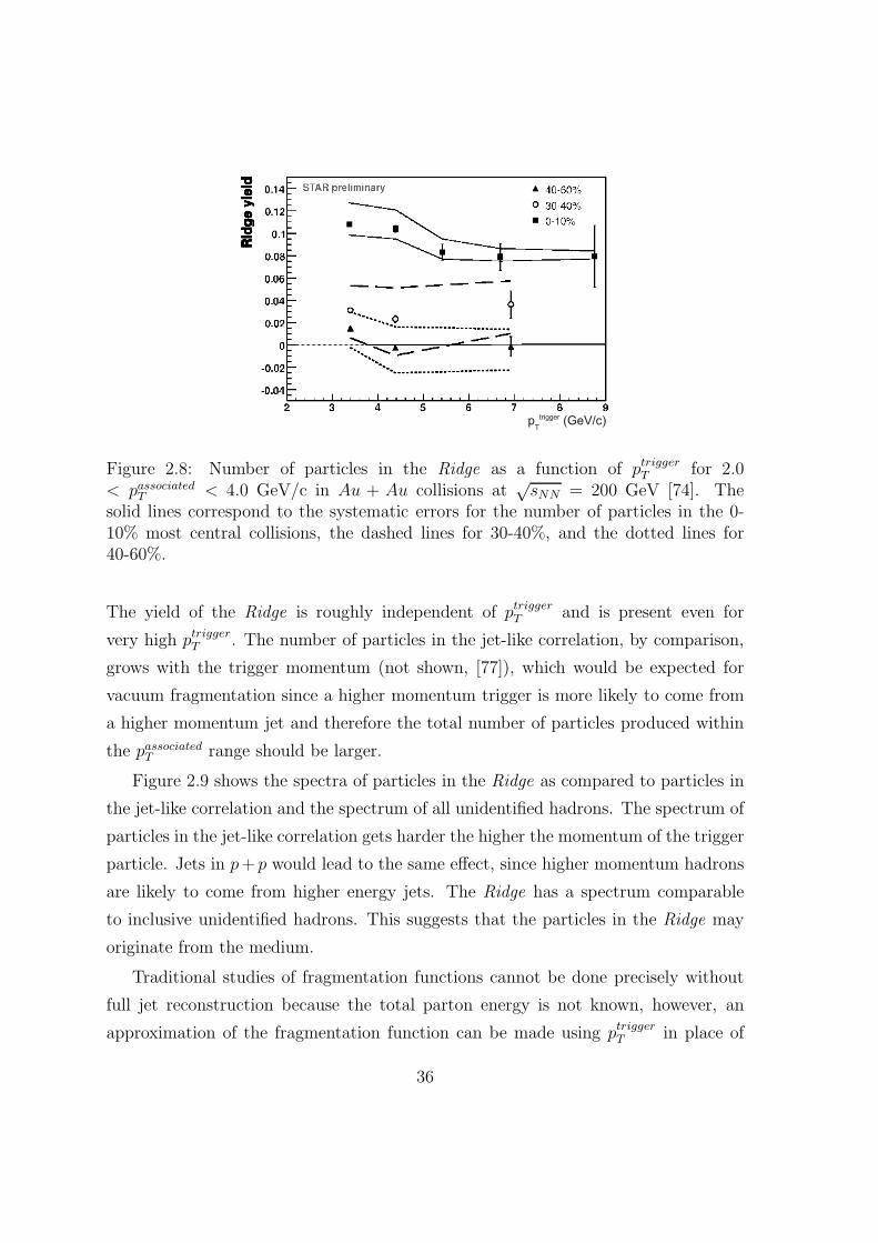
Figure 2.8: Number of particles in the Ridge as a function of ptriggerT for 2.0

< passociatedT < 4.0 GeV/c in Au + Au collisions at

√sNN = 200 GeV [74]. The

solid lines correspond to the systematic errors for the number of particles in the 0-10% most central collisions, the dashed lines for 30-40%, and the dotted lines for40-60%.

The yield of the Ridge is roughly independent of ptriggerT and is present even for

very high ptriggerT . The number of particles in the jet-like correlation, by comparison,

grows with the trigger momentum (not shown, [77]), which would be expected for

vacuum fragmentation since a higher momentum trigger is more likely to come from

a higher momentum jet and therefore the total number of particles produced within

the passociatedT range should be larger.

Figure 2.9 shows the spectra of particles in the Ridge as compared to particles in

the jet-like correlation and the spectrum of all unidentified hadrons. The spectrum of

particles in the jet-like correlation gets harder the higher the momentum of the trigger

particle. Jets in p+ p would lead to the same effect, since higher momentum hadrons

are likely to come from higher energy jets. The Ridge has a spectrum comparable

to inclusive unidentified hadrons. This suggests that the particles in the Ridge may

originate from the medium.

Traditional studies of fragmentation functions cannot be done precisely without

full jet reconstruction because the total parton energy is not known, however, an

approximation of the fragmentation function can be made using ptriggerT in place of

36

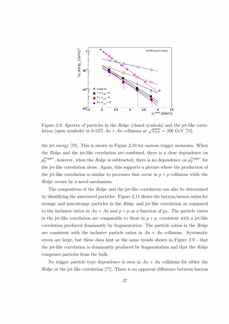
Figure 2.9: Spectra of particles in the Ridge (closed symbols) and the jet-like corre-lation (open symbols) in 0-12% Au+ Au collisions at

√sNN = 200 GeV [74].

the jet energy [78]. This is shown in Figure 2.10 for various trigger momenta. When

the Ridge and the jet-like correlation are combined, there is a clear dependence on

ptriggerT , however, when the Ridge is subtracted, there is no dependence on ptrigger

T for

the jet-like correlation alone. Again, this supports a picture where the production of

the jet-like correlation is similar to processes that occur in p + p collisions while the

Ridge occurs by a novel mechanism.

The composition of the Ridge and the jet-like correlation can also be determined

by identifying the associated particles. Figure 2.11 shows the baryon/meson ratios for

strange and non-strange particles in the Ridge and jet-like correlation as compared

to the inclusive ratios in Au+ Au and p + p as a function of pT . The particle ratios

in the jet-like correlation are comparable to those in p+ p, consistent with a jet-like

correlation produced dominantly by fragmentation. The particle ratios in the Ridge

are consistent with the inclusive particle ratios in Au + Au collisions. Systematic

errors are large, but these data hint at the same trends shown in Figure 2.9 - that

the jet-like correlation is dominantly produced by fragmentation and that the Ridge

comprises particles from the bulk.

No trigger particle type dependence is seen in Au + Au collisions for either the

Ridge or the jet-like correlation [77]. There is no apparent difference between baryon

37

Figure 2.10: Di-hadron fragmentation function zT = pT

ptriggerT

with and without Ridge

subtraction in 0-12% central Au + Au collisions at√sNN = 200 GeV [74] (a) shows

the di-hadron fragmentation for the jet-like correlation and the Ridge combined. (b)shows the di-hadron fragmentation function for the jet-like correlation alone aftersubtracting the Ridge. (c) shows the ratio of the di-hadron fragmentation functionfor the jet-like correlation alone to the di-hadron fragmentation function measured ind+ Au.

and meson triggers, even though there are dramatic differences between baryons

and mesons in nuclear modification factors (shown in Figure 1.19) and azimuthal

anisotropies (shown in Figure 1.17). A trigger particle dependence might be expected

if there were a dramatic difference between quark and gluon jets, as the rates of

production of Λ and Λ are comparable in gluon jets but many more Λ than Λ are

38

(GeV/c)assocTp

0 1 2 3 4 5 6

S0/K

Λ

0

0.5

1

1.5

2

2.5, 0-5% Au+Au

Tinclusive p

, 20-40% Au+Au T

inclusive p, p+p

Tinclusive p

ridge, 0-10% Au+Aujet, 0-10% Au+Au

STAR preliminary

Figure 2.11: Comparisons of the Λ/K0S ratio (left) [79] and of the p/π ratio (right) [80]

in the Ridge and the jet-like correlation to the inclusive ratios. Systematic errors areadded in quadrature to the statistical errors for the Λ/K0

S ratio and shown as bandsfor the p/π ratio.

(deg)RP

Ψ-T

φ=sφ

0 20 40 60 80

Yie

ld

0

0.05

0.1

0.15

0.2

dAu

jet part, near-side

ridge part, near-side

(deg)RPΨ-Tφ=

sφ

0 20 40 60 80

Yie

ld

0

0.05

0.1

0.15

0.2

dAu

jet part, near-side

ridge part, near-side

Figure 2.12: Reaction plane dependence of number of particles in the jet-like cor-relation and the Ridge for 0-5% central (left) and 20-60% central (right) Au + Aucollisions at

√sNN = 200 GeV [82]. The lines correspond to the systematic errors on

the number of particles in the Ridge. The arrow corresponds to the reaction planeaveraged jet-like yield in d+ Au. The lines correspond to the systematic errors.

predicted to be produced by quark jets. No difference between Λ and Λ trigger par-

ticles is observed (not shown). This independence of the yield on the trigger particle

type extends even to the Ω− [81].

39

1η∆

-1.5 -1 -0.5 0 0.5 1 1.5

2η

∆

-1.5

-1

-0.5

0

0.5

1

1.5

-0.2

-0.1

0

0.1

0.2

0.3

0.4

0.5d+Au

(a)STAR Preliminary

1η∆

-1.5 -1 -0.5 0 0.5 1 1.5

2η

∆

-1.5

-1

-0.5

0

0.5

1

1.5

-0.2

-0.1

0

0.1

0.2

0.3

0.4

0.540-80%Au+Au

(b)STAR Preliminary

1η∆

-1.5 -1 -0.5 0 0.5 1 1.5

2η

∆

-1.5

-1

-0.5

0

0.5

1

1.5

2η

∆d 1

η∆

N/d

2d

-0.2

-0.1

0

0.1

0.2

0.3

0.4

0.50-12%Au+Au

(c)STAR Preliminary

Figure 2.13: 3-particle correlations for 3.0 < ptriggerT < 10.0 GeV/c and 1.0 <

passociatedT < 3.0 GeV/c for both associated particles on the near-side in d + Au,

peripheral Au+ Au, and central Au+ Au collisions at√sNN = 200 GeV [83].

Figure 2.12 shows the reaction plane dependence of the Ridge and the jet-like

correlations in two different centrality bins. The jet-like correlation shows little de-

pendence on the direction relative to the reaction plane, as would be expected if

the jet-like correlation originates from vacuum fragmentation. The Ridge is largest

in plane, where the mean path length traveled by the parton would be shortest. If

the Ridge is produced by parton energy loss, these results would indicate that jets

produced out of plane are either produced on the surface or completely quenched.

Additionally, measurements were done to determine if particles in the Ridge are

correlated with each other. 3-particle correlations on the near-side are shown in

Figure 2.13. A trigger particle with 3.0 < ptriggerT < 10.0 GeV/c is selected and

defines the origin. Only events with at least two associated particles in the range

1.0 < passociatedT < 3.0 GeV/c are selected and Figure 2.13 shows the location of

the first associated particle relative to the trigger versus the location of the second

associated particle relative to the trigger. A narrow peak around the trigger particle

is observed in the d+Au, peripheral Au+Au, and central Au+Au data and comes

from the same process that produces the jet-like correlation in di-hadron correlations.

In the Au + Au, this peak sits on top of a plateau; this is the Ridge. If the two

associated particles came from the same source - for instance, from gluon radiation -

they would be expected to be correlated in space. Instead, within the the acceptance

of the detector and the statistical errors, particles in the Ridge do not appear to be

correlated. However, an understanding of the effects of the kinematic cuts is required

40

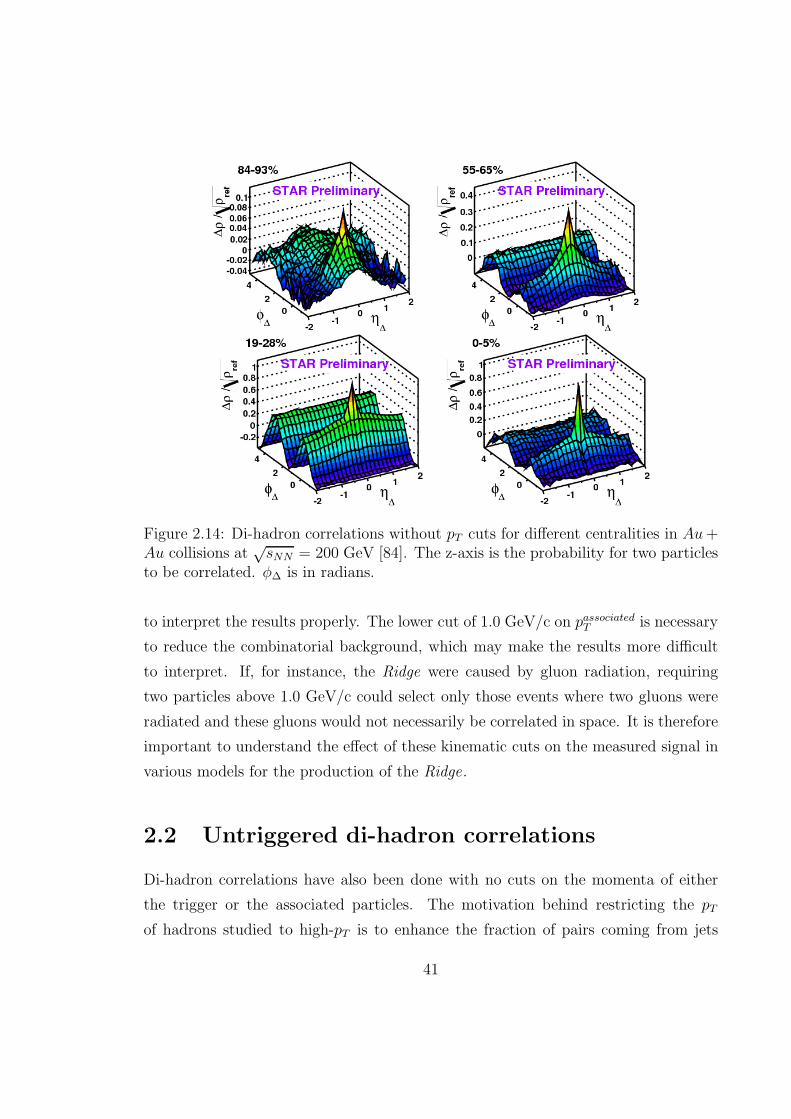
Figure 2.14: Di-hadron correlations without pT cuts for different centralities in Au+Au collisions at

√sNN = 200 GeV [84]. The z-axis is the probability for two particles

to be correlated. φ∆ is in radians.

to interpret the results properly. The lower cut of 1.0 GeV/c on passociatedT is necessary

to reduce the combinatorial background, which may make the results more difficult

to interpret. If, for instance, the Ridge were caused by gluon radiation, requiring

two particles above 1.0 GeV/c could select only those events where two gluons were

radiated and these gluons would not necessarily be correlated in space. It is therefore

important to understand the effect of these kinematic cuts on the measured signal in

various models for the production of the Ridge.

2.2 Untriggered di-hadron correlations

Di-hadron correlations have also been done with no cuts on the momenta of either

the trigger or the associated particles. The motivation behind restricting the pT

of hadrons studied to high-pT is to enhance the fraction of pairs coming from jets

41

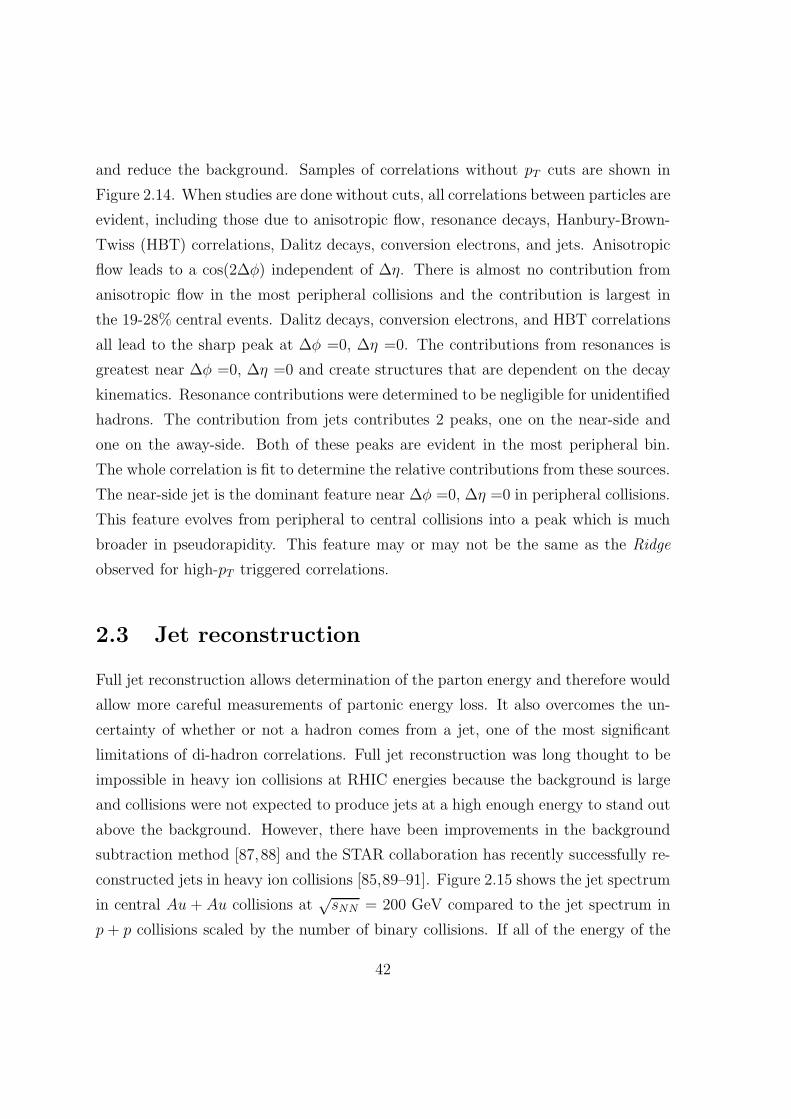
and reduce the background. Samples of correlations without pT cuts are shown in

Figure 2.14. When studies are done without cuts, all correlations between particles are

evident, including those due to anisotropic flow, resonance decays, Hanbury-Brown-

Twiss (HBT) correlations, Dalitz decays, conversion electrons, and jets. Anisotropic

flow leads to a cos(2∆φ) independent of ∆η. There is almost no contribution from

anisotropic flow in the most peripheral collisions and the contribution is largest in

the 19-28% central events. Dalitz decays, conversion electrons, and HBT correlations

all lead to the sharp peak at ∆φ =0, ∆η =0. The contributions from resonances is

greatest near ∆φ =0, ∆η =0 and create structures that are dependent on the decay

kinematics. Resonance contributions were determined to be negligible for unidentified

hadrons. The contribution from jets contributes 2 peaks, one on the near-side and

one on the away-side. Both of these peaks are evident in the most peripheral bin.

The whole correlation is fit to determine the relative contributions from these sources.

The near-side jet is the dominant feature near ∆φ =0, ∆η =0 in peripheral collisions.

This feature evolves from peripheral to central collisions into a peak which is much

broader in pseudorapidity. This feature may or may not be the same as the Ridge

observed for high-pT triggered correlations.

2.3 Jet reconstruction

Full jet reconstruction allows determination of the parton energy and therefore would

allow more careful measurements of partonic energy loss. It also overcomes the un-

certainty of whether or not a hadron comes from a jet, one of the most significant

limitations of di-hadron correlations. Full jet reconstruction was long thought to be

impossible in heavy ion collisions at RHIC energies because the background is large

and collisions were not expected to produce jets at a high enough energy to stand out

above the background. However, there have been improvements in the background

subtraction method [87,88] and the STAR collaboration has recently successfully re-

constructed jets in heavy ion collisions [85,89–91]. Figure 2.15 shows the jet spectrum

in central Au + Au collisions at√sNN = 200 GeV compared to the jet spectrum in

p + p collisions scaled by the number of binary collisions. If all of the energy of the

42

Figure 2.15: Reconstructed jet spectrum in central Au+Au collisions at√sNN = 200

GeV as compared to the jet spectrum in p+ p scaled by Nbin [85,86]. Only statisticalerrors are shown for Au+ Au data. The systematic errors on the overall scale of thep+ p spectrum are 50%.

jet is measured, the spectra in Au+Au and in p+ p collisions scaled by Nbin should

be the same, as it appears to be. This does not mean that the parton did not lose

energy, only that this energy must appear somewhere because of energy conservation.

The systematic error on the p+ p spectrum is 50% [86] and the systematic errors on

the Au+Au spectrum are not yet determined. The jets’ shape in azimuth and pseu-

dorapidity could still be modified and the fragmentation functions are not necessarily

vacuum fragmentation functions.

Jet reconstruction and correlation studies are complementary. If the shape is

changed too dramatically, jet reconstruction algorithms may not recognize the mod-

ified jets. Additionally, some studies of rare particles in jets are best suited to corre-

lation studies due to statistics.

43

2.4 Summary

Studies of di-hadron correlations and nuclear modification factors at RHIC have

demonstrated that jets are considerably modified by the medium. This could be

through partonic energy loss before fragmentation or through modification of the

fragmentation functions in the medium. These modifications have typically been

classified as being on the near-side or the away-side. A note of caution is warranted

since the near-side and the away-side are defined only by their relation to the trigger

particle and the only indication that the trigger particle might come from a jet is its

momentum.

For an intermediate pT trigger (roughly 3.0 < ptriggerT < 6.0 GeV/c), particles on

the away-side are observed at lower momentum than in p + p and d + Au collisions.

The away-side is not observed at passociatedT ≈ 2 GeV/c (Figure 2.3), but at lower

momenta the away-side is broadened and develops a double-peaked structure (Fig-

ure 2.4). When the momenta of the trigger and associated particles are increased,

the away-side reappears (Figure 2.5); this is interpreted as a greater bias towards

unmodified jet fragmentation, perhaps through greater surface bias. The Ridge is

the dominant feature on the near-side for intermediate pT triggers (Figure 2.6). It

persists out to ptriggerT ≈ 8 GeV/c, however, a greater percentage of the particles

correlated with the trigger particle are in the jet-like correlation (Figure 2.8). As

passociatedT is increased, a greater percentage of the particles correlated with the trigger

particle are in the jet-like correlation (Figure 2.9); at lower passociatedT , measurements

are overwhelmed by systematic errors and precise data are unavailable. The features

observed in correlation studies are momentum dependent, presumably reflecting dif-

ferences in the relative importance of various mechanisms which produce correlations

as a function of pT .

The jet-like correlation shows the Npart, passociatedT , and ptrigger

T dependence that

would be expected from vacuum fragmentation, although a more quantitative under-

standing of the jet-like correlation is needed. The Ridge is a new feature that appears

to be made of particles from the bulk due to its similar composition (Figure 2.11).

44

The spectra of particles in the Ridge are comparable to the inclusive spectra of par-

ticles, and the ratios of particles in the Ridge are similar to those in the bulk. The

Ridge is clearly correlated in space with a high-pT particle, but that does not prove

that the production of the two are related. The full breadth of the data and an under-

standing of various models for the production of the Ridge are necessary to determine

what this feature is, where it comes from, and what it can tell us about the QGP

and relativistic heavy ion collisions. The studies presented in this thesis will add

to our understanding of the jet-like correlation and the Ridge by investigating their

dependence on collision energy and system size and their particle type dependence.

45

46

Chapter 3

Experiment

3.1 The Relativistic Heavy Ion Collider

The Relativistic Heavy Ion Collider (RHIC) is located in Upton, NY on Long Island

and is approximately 1.2 km in diameter. An aerial view of RHIC is shown in Fig-

ure 3.1. RHIC spans nearly two orders of magnitude in collision energy per nucleon.

RHIC was designed to collide nuclei with an atomic mass, A, ranging from A = 1 to

A ≈ 200. It is also capable of asymmetric collisions, those between ions with differ-

ent masses, such as d + Au. Asymmetric collisions are useful for distinguishing the

effects of cold nuclear matter (modification of the initial state in a nucleus) versus

hot nuclear matter (such as a QGP). To date RHIC has taken data from the collision

energies and systems shown in Table 3.1. RHIC is also the only collider in the world

capable of colliding both longitudinally and transversely polarized protons. Polarized

proton collisions are used to study the origin of the spin of the proton. RHIC has

now collided polarized protons at 500 GeV. Design specifications for RHIC are listed

in Table 3.2. These specifications have now been exceeded. Au + Au collisions can

reach energies as low as 2.5 GeV/u. p + p collisions with up to 109 bunches in each

ring and at luminosities of up to 9 x 1031 cm−2 s−1 were obtained in the 2009 run.

The ion beams are created by stripping the electrons off of the nuclei and acceler-

ating the nuclei to their full energy in several stages. For gold ions, negatively charged

47

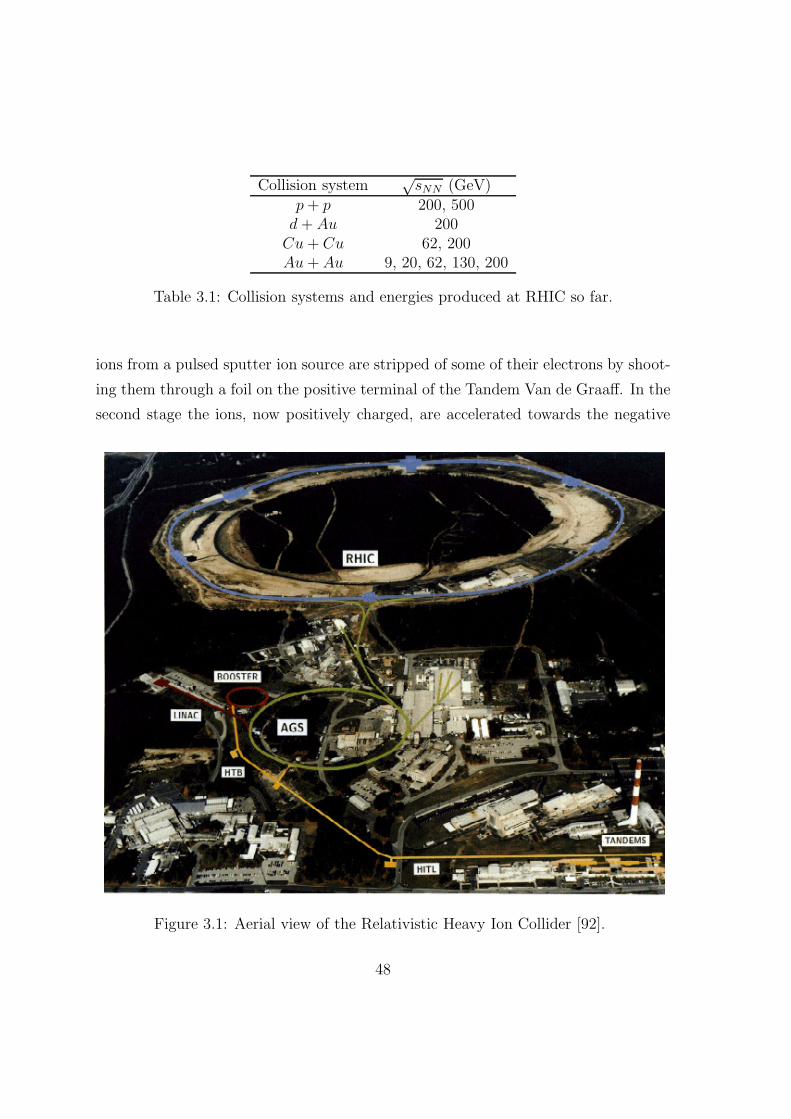
Collision system√sNN (GeV)

p+ p 200, 500d+ Au 200Cu+ Cu 62, 200Au+ Au 9, 20, 62, 130, 200

Table 3.1: Collision systems and energies produced at RHIC so far.

ions from a pulsed sputter ion source are stripped of some of their electrons by shoot-

ing them through a foil on the positive terminal of the Tandem Van de Graaff. In the

second stage the ions, now positively charged, are accelerated towards the negative

Figure 3.1: Aerial view of the Relativistic Heavy Ion Collider [92].

48

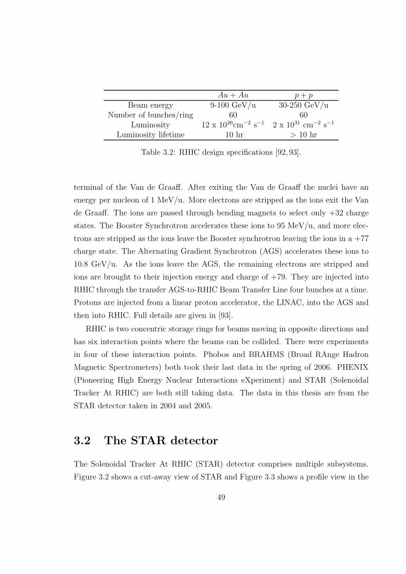
Au+ Au p+ pBeam energy 9-100 GeV/u 30-250 GeV/u

Number of bunches/ring 60 60Luminosity 12 x 1026cm−2 s−1 2 x 1031 cm−2 s−1

Luminosity lifetime 10 hr > 10 hr

Table 3.2: RHIC design specifications [92, 93].

terminal of the Van de Graaff. After exiting the Van de Graaff the nuclei have an

energy per nucleon of 1 MeV/u. More electrons are stripped as the ions exit the Van

de Graaff. The ions are passed through bending magnets to select only +32 charge

states. The Booster Synchrotron accelerates these ions to 95 MeV/u, and more elec-

trons are stripped as the ions leave the Booster synchrotron leaving the ions in a +77

charge state. The Alternating Gradient Synchrotron (AGS) accelerates these ions to

10.8 GeV/u. As the ions leave the AGS, the remaining electrons are stripped and

ions are brought to their injection energy and charge of +79. They are injected into

RHIC through the transfer AGS-to-RHIC Beam Transfer Line four bunches at a time.

Protons are injected from a linear proton accelerator, the LINAC, into the AGS and

then into RHIC. Full details are given in [93].

RHIC is two concentric storage rings for beams moving in opposite directions and

has six interaction points where the beams can be collided. There were experiments

in four of these interaction points. Phobos and BRAHMS (Broad RAnge Hadron

Magnetic Spectrometers) both took their last data in the spring of 2006. PHENIX

(Pioneering High Energy Nuclear Interactions eXperiment) and STAR (Solenoidal

Tracker At RHIC) are both still taking data. The data in this thesis are from the

STAR detector taken in 2004 and 2005.

3.2 The STAR detector

The Solenoidal Tracker At RHIC (STAR) detector comprises multiple subsystems.

Figure 3.2 shows a cut-away view of STAR and Figure 3.3 shows a profile view in the

49

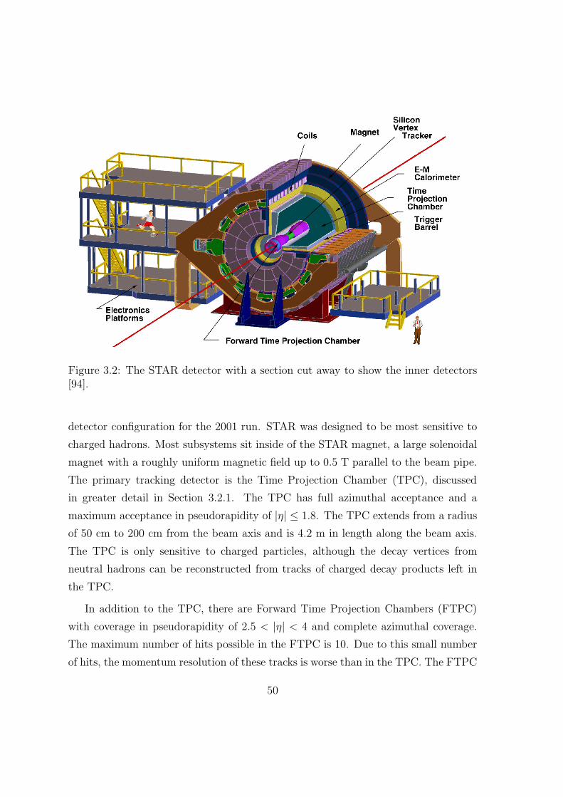
Figure 3.2: The STAR detector with a section cut away to show the inner detectors[94].

detector configuration for the 2001 run. STAR was designed to be most sensitive to

charged hadrons. Most subsystems sit inside of the STAR magnet, a large solenoidal

magnet with a roughly uniform magnetic field up to 0.5 T parallel to the beam pipe.

The primary tracking detector is the Time Projection Chamber (TPC), discussed

in greater detail in Section 3.2.1. The TPC has full azimuthal acceptance and a

maximum acceptance in pseudorapidity of |η| ≤ 1.8. The TPC extends from a radius

of 50 cm to 200 cm from the beam axis and is 4.2 m in length along the beam axis.

The TPC is only sensitive to charged particles, although the decay vertices from

neutral hadrons can be reconstructed from tracks of charged decay products left in

the TPC.

In addition to the TPC, there are Forward Time Projection Chambers (FTPC)

with coverage in pseudorapidity of 2.5 < |η| < 4 and complete azimuthal coverage.

The maximum number of hits possible in the FTPC is 10. Due to this small number

of hits, the momentum resolution of these tracks is worse than in the TPC. The FTPC

50

Figure 3.3: A profile view of the STAR detector [94]. This was the detector configu-ration for the Cu+ Cu run in 2005.

can also be used to determine the reaction plane.

There are two silicon detectors, the Silicon Vertex Tracker (SVT) and the Silicon

Strip Detector (SSD) inside the inner field cage of the TPC. These detectors have hit

resolutions of approximately 100 µm and 200 µm, respectively. The three layers of

the SVT range from radii of 7, 11, and 15 cm from the beam pipe. The single silicon

layer SSD is located at 23 cm radially from the beam pipe. These silicon detectors

have the capacity to provide more accurate tracking closer to the beam pipe, but

these detectors were only used in the 2005 run and later.

There are two electromagnetic calorimeters that can be used for measurements of

electrons, photons, and triggering. The Barrel Electromagnetic Calorimeter (BEMC)

has full acceptance in azimuth and an acceptance of |η| < 1. The Endcap Electro-

magnetic Calorimeters (EEMC) have full azimuthal acceptance and an acceptance

of 1 < η < 2. All electromagnetic calorimeters have shower maximum detectors to

distinguish signals left by hadrons from those left by photons and electrons.

51

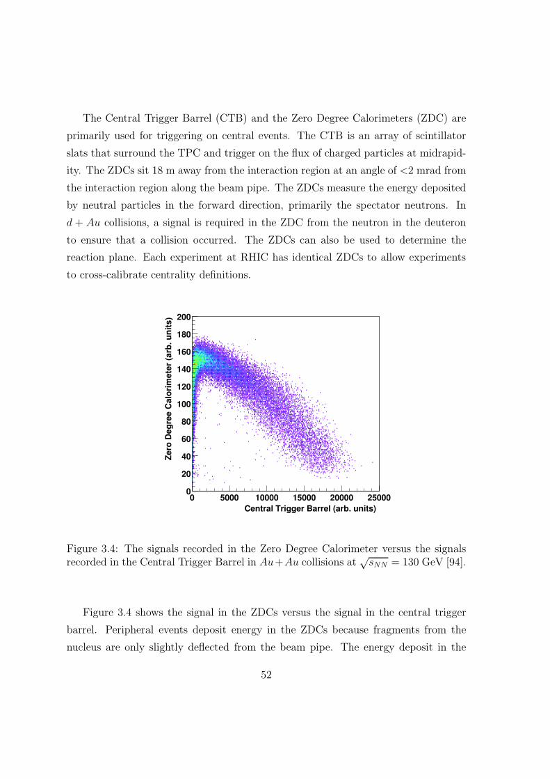
The Central Trigger Barrel (CTB) and the Zero Degree Calorimeters (ZDC) are

primarily used for triggering on central events. The CTB is an array of scintillator

slats that surround the TPC and trigger on the flux of charged particles at midrapid-

ity. The ZDCs sit 18 m away from the interaction region at an angle of <2 mrad from

the interaction region along the beam pipe. The ZDCs measure the energy deposited

by neutral particles in the forward direction, primarily the spectator neutrons. In

d + Au collisions, a signal is required in the ZDC from the neutron in the deuteron

to ensure that a collision occurred. The ZDCs can also be used to determine the

reaction plane. Each experiment at RHIC has identical ZDCs to allow experiments

to cross-calibrate centrality definitions.

Central Trigger Barrel (arb. units)

0 5000 10000 15000 20000 25000

Zero

Deg

ree C

alo

rim

ete

r (a

rb. u

nit

s)

0

20

40

60

80

100

120

140

160

180

200

Figure 3.4: The signals recorded in the Zero Degree Calorimeter versus the signalsrecorded in the Central Trigger Barrel in Au+Au collisions at

√sNN = 130 GeV [94].

Figure 3.4 shows the signal in the ZDCs versus the signal in the central trigger

barrel. Peripheral events deposit energy in the ZDCs because fragments from the

nucleus are only slightly deflected from the beam pipe. The energy deposit in the

52

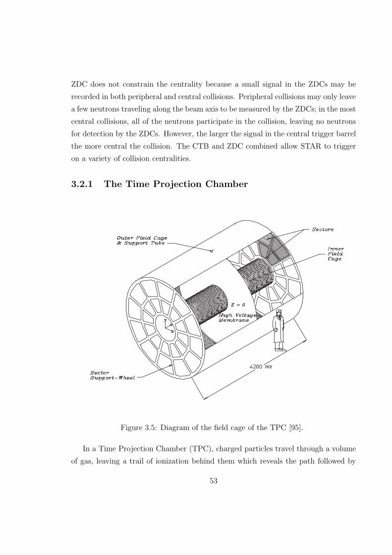
ZDC does not constrain the centrality because a small signal in the ZDCs may be

recorded in both peripheral and central collisions. Peripheral collisions may only leave

a few neutrons traveling along the beam axis to be measured by the ZDCs; in the most

central collisions, all of the neutrons participate in the collision, leaving no neutrons

for detection by the ZDCs. However, the larger the signal in the central trigger barrel

the more central the collision. The CTB and ZDC combined allow STAR to trigger

on a variety of collision centralities.

3.2.1 The Time Projection Chamber

Figure 3.5: Diagram of the field cage of the TPC [95].

In a Time Projection Chamber (TPC), charged particles travel through a volume

of gas, leaving a trail of ionization behind them which reveals the path followed by

53

the particle. The STAR TPC is cylindrical around the beam pipe and sits inside the

STAR magnet with a magnetic field of up to 0.5 T parallel to the beam pipe. The

TPC central membrane and field cage create an electric field of 135 V/cm that is

parallel to the beam pipe. The TPC is 4.2 m long with an outer diameter of 4 m and

an inner diameter of 1 m. The magnetic field bends charged particles as they move

through the TPC, allowing determination of momentum.

When a charged particle travels through the TPC, it knocks off electrons from

the molecules in the gas. These ionization electrons are accelerated through the TPC

by the electric field until they reach a constant speed which is a characteristic of the

gas and the electric field. They move roughly two orders of magnitude faster than

the ionized gas and therefore will be collected first. For sufficiently low event rates,

the ions can be neglected; for higher rates of events, ions can create significant local

distortions in the electric field that alter the trajectory of nearby ionization electrons

and can impair momentum resolution unless these field distortions are corrected for.

The position in the plane perpendicular to the beam (the x-y plane) is determined

by the location where the ionization electrons are collected on the readout pads.

The position in the direction along the beam axis (the z-axis) is determined by the

time that it takes the ionization electrons to reach the endcap, hence the name Time

Projection Chamber.

A significant advantage of the TPC is its low material budget (2.43% X0) which

reduces the probability of photon conversion as they pass through the TPC and

reduces the probability for hadrons to scatter in the TPC. The drift volume of the

TPC is filled with P10 gas (10% methane and 90% argon) held at 2 mbar above

atmospheric pressure. The slight overpressure reduces impurities in the gas since any

leaks will cause P10 to leak out instead of causing air to leak in. Water and oxygen

dramatically change the drift velocity of electrons and can capture electrons, reducing

the efficiency of the response of the TPC to charged particles. Operating the TPC

near the maximum electron drift speed reduces the effect of symmetry magazine slight

fluctuations in the electric field. P10 gas has its maximum electron drift speed (5.45

cm/s) at a relatively low electric field, reducing the overall electric field needed.

The drift volume sits in a uniform field of ≈ 135 V/cm created by the field cage of

54

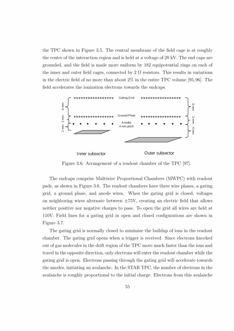
the TPC shown in Figure 3.5. The central membrane of the field cage is at roughly

the center of the interaction region and is held at a voltage of 28 kV. The end caps are

grounded, and the field is made more uniform by 182 equipotential rings on each of

the inner and outer field cages, connected by 2 Ω resistors. This results in variations

in the electric field of no more than about 2% in the entire TPC volume [95,96]. The

field accelerates the ionization electrons towards the endcaps.

Anodes

4 mm pitch

Ground Plane

Inner subsector Outer subsector

Gating Grid

4 m

m2

mm

6 m

m

2 m

m2

mm

6 m

m

Figure 3.6: Arrangement of a readout chamber of the TPC [97].

The endcaps comprise Multiwire Proportional Chambers (MWPC) with readout

pads, as shown in Figure 3.6. The readout chambers have three wire planes, a gating

grid, a ground plane, and anode wires. When the gating grid is closed, voltages

on neighboring wires alternate between ±75V, creating an electric field that allows

neither positive nor negative charges to pass. To open the grid all wires are held at

110V. Field lines for a gating grid in open and closed configurations are shown in

Figure 3.7.

The gating grid is normally closed to minimize the buildup of ions in the readout

chamber. The gating grid opens when a trigger is received. Since electrons knocked

out of gas molecules in the drift region of the TPC move much faster than the ions and

travel in the opposite direction, only electrons will enter the readout chamber while the

gating grid is open. Electrons passing through the gating grid will accelerate towards

the anodes, initiating an avalanche. In the STAR TPC, the number of electrons in the

avalanche is roughly proportional to the initial charge. Electrons from this avalanche

55

–0.6 –0.4 –0.2 0.20 0.4 0.6x (cm)

y (

cm)

y (

cm)

0.6

0.8

2.0

1.0

1.2

1.4

1.6

1.8

0.4

0.6

0.8

1.0

1.2

1.4

1.6

1.8 (b) Gating grid open

(a) Gating grid closed

gating grid

shielding grid

anode wires

cathode plane

+− +− +− −

Figure 3.7: Field lines for a gating grid in the (a) closed and (b) open configurations[98].

are collected on the wires, but a cloud of positively charged ions remains. An image

charge will form on the readout plane and it is the image charge that is recorded.

The width of the cloud of charge in the STAR TPC is diffused by 185 µm/√cm

and 320 µm/√cm traveled through TPC in the transverse and longitudinal directions,

respectively. The width of the image charge collected on the readout pad is also

dependent on the dip angle and crossing angle of the track. The dip angle is the

angle between the particle’s momentum and the drift direction. The crossing angle is

that between the particle’s momentum and the direction normal to the pad row. The

size of the image charge is smallest for short drift distances, small crossing angles, and

small dip angles. The average width of the image charge is 350 µm in the transverse

direction and 700 µm in the longitudinal direction, smaller than the typical TPC pad.

56

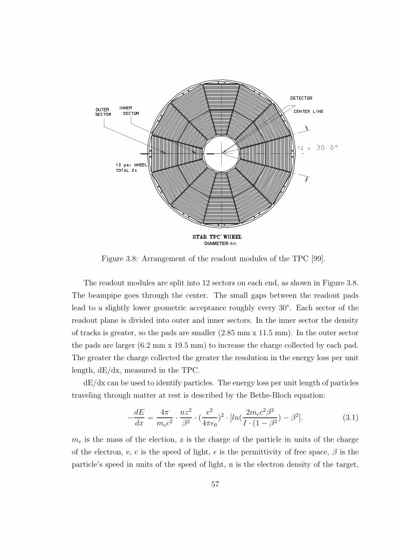
DIAMETER 4m

Figure 3.8: Arrangement of the readout modules of the TPC [99].

The readout modules are split into 12 sectors on each end, as shown in Figure 3.8.

The beampipe goes through the center. The small gaps between the readout pads

lead to a slightly lower geometric acceptance roughly every 30°. Each sector of the

readout plane is divided into outer and inner sectors. In the inner sector the density

of tracks is greater, so the pads are smaller (2.85 mm x 11.5 mm). In the outer sector

the pads are larger (6.2 mm x 19.5 mm) to increase the charge collected by each pad.

The greater the charge collected the greater the resolution in the energy loss per unit

length, dE/dx, measured in the TPC.

dE/dx can be used to identify particles. The energy loss per unit length of particles

traveling through matter at rest is described by the Bethe-Bloch equation:

−dEdx

=4π

mec2· nz

2

β2· ( e2

4πǫ0)2 · [ln(

2mec2β2

I · (1 − β2) − β2]. (3.1)

me is the mass of the election, z is the charge of the particle in units of the charge

of the electron, e, c is the speed of light, ǫ is the permittivity of free space, β is the

particle’s speed in units of the speed of light, n is the electron density of the target,

57

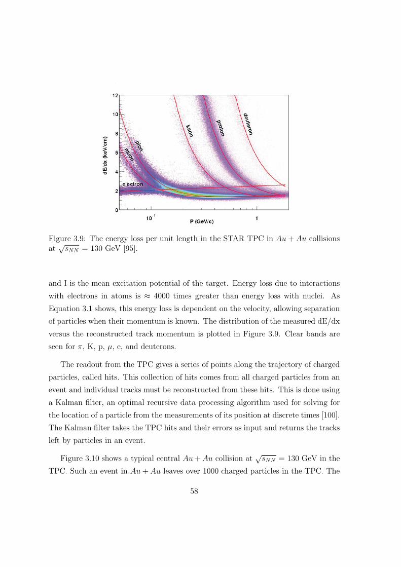
Figure 3.9: The energy loss per unit length in the STAR TPC in Au+ Au collisionsat

√sNN = 130 GeV [95].

and I is the mean excitation potential of the target. Energy loss due to interactions

with electrons in atoms is ≈ 4000 times greater than energy loss with nuclei. As

Equation 3.1 shows, this energy loss is dependent on the velocity, allowing separation

of particles when their momentum is known. The distribution of the measured dE/dx

versus the reconstructed track momentum is plotted in Figure 3.9. Clear bands are

seen for π, K, p, µ, e, and deuterons.

The readout from the TPC gives a series of points along the trajectory of charged

particles, called hits. This collection of hits comes from all charged particles from an

event and individual tracks must be reconstructed from these hits. This is done using

a Kalman filter, an optimal recursive data processing algorithm used for solving for

the location of a particle from the measurements of its position at discrete times [100].

The Kalman filter takes the TPC hits and their errors as input and returns the tracks

left by particles in an event.

Figure 3.10 shows a typical central Au+Au collision at√sNN = 130 GeV in the

TPC. Such an event in Au+ Au leaves over 1000 charged particles in the TPC. The

58

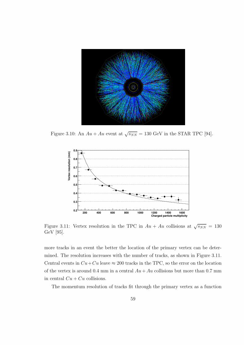
Figure 3.10: An Au+ Au event at√sNN = 130 GeV in the STAR TPC [94].

Charged particle multiplicity200 400 600 800 1000 1200 1400 1600

Ve

rte

x r

es

olu

tio

n (

mm

)

0.2

0.3

0.4

0.5

0.6

0.7

0.8

0.9

Figure 3.11: Vertex resolution in the TPC in Au + Au collisions at√sNN = 130

GeV [95].

more tracks in an event the better the location of the primary vertex can be deter-

mined. The resolution increases with the number of tracks, as shown in Figure 3.11.

Central events in Cu+Cu leave ≈ 200 tracks in the TPC, so the error on the location

of the vertex is around 0.4 mm in a central Au+Au collisions but more than 0.7 mm

in central Cu+ Cu collisions.

The momentum resolution of tracks fit through the primary vertex as a function

59

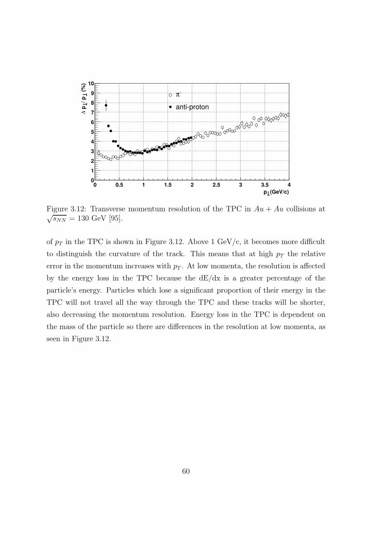
(GeV/c)p

0 0.5 1 1.5 2 2.5 3 3.5 4

(

%)

/ p

p∆

0

1

2

3

4

5

6

7

8

9

10

-π

anti-proton

Figure 3.12: Transverse momentum resolution of the TPC in Au + Au collisions at√sNN = 130 GeV [95].

of pT in the TPC is shown in Figure 3.12. Above 1 GeV/c, it becomes more difficult

to distinguish the curvature of the track. This means that at high pT the relative

error in the momentum increases with pT . At low momenta, the resolution is affected

by the energy loss in the TPC because the dE/dx is a greater percentage of the

particle’s energy. Particles which lose a significant proportion of their energy in the

TPC will not travel all the way through the TPC and these tracks will be shorter,

also decreasing the momentum resolution. Energy loss in the TPC is dependent on

the mass of the particle so there are differences in the resolution at low momenta, as

seen in Figure 3.12.

60

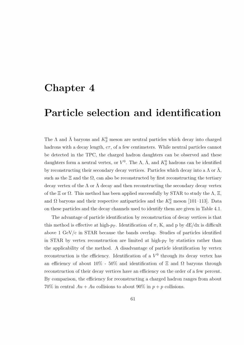
Chapter 4

Particle selection and identification

The Λ and Λ baryons and K0S meson are neutral particles which decay into charged

hadrons with a decay length, cτ , of a few centimeters. While neutral particles cannot

be detected in the TPC, the charged hadron daughters can be observed and these

daughters form a neutral vertex, or V 0. The Λ, Λ, and K0S hadrons can be identified

by reconstructing their secondary decay vertices. Particles which decay into a Λ or Λ,

such as the Ξ and the Ω, can also be reconstructed by first reconstructing the tertiary

decay vertex of the Λ or Λ decay and then reconstructing the secondary decay vertex

of the Ξ or Ω. This method has been applied successfully by STAR to study the Λ, Ξ,

and Ω baryons and their respective antiparticles and the K0S meson [101–113]. Data

on these particles and the decay channels used to identify them are given in Table 4.1.

The advantage of particle identification by reconstruction of decay vertices is that

this method is effective at high-pT . Identification of π, K, and p by dE/dx is difficult

above 1 GeV/c in STAR because the bands overlap. Studies of particles identified

in STAR by vertex reconstruction are limited at high-pT by statistics rather than

the applicability of the method. A disadvantage of particle identification by vertex

reconstruction is the efficiency. Identification of a V 0 through its decay vertex has

an efficiency of about 10% - 50% and identification of Ξ and Ω baryons through

reconstruction of their decay vertices have an efficiency on the order of a few percent.

By comparison, the efficiency for reconstructing a charged hadron ranges from about

70% in central Au+ Au collisions to about 90% in p+ p collisions.

61

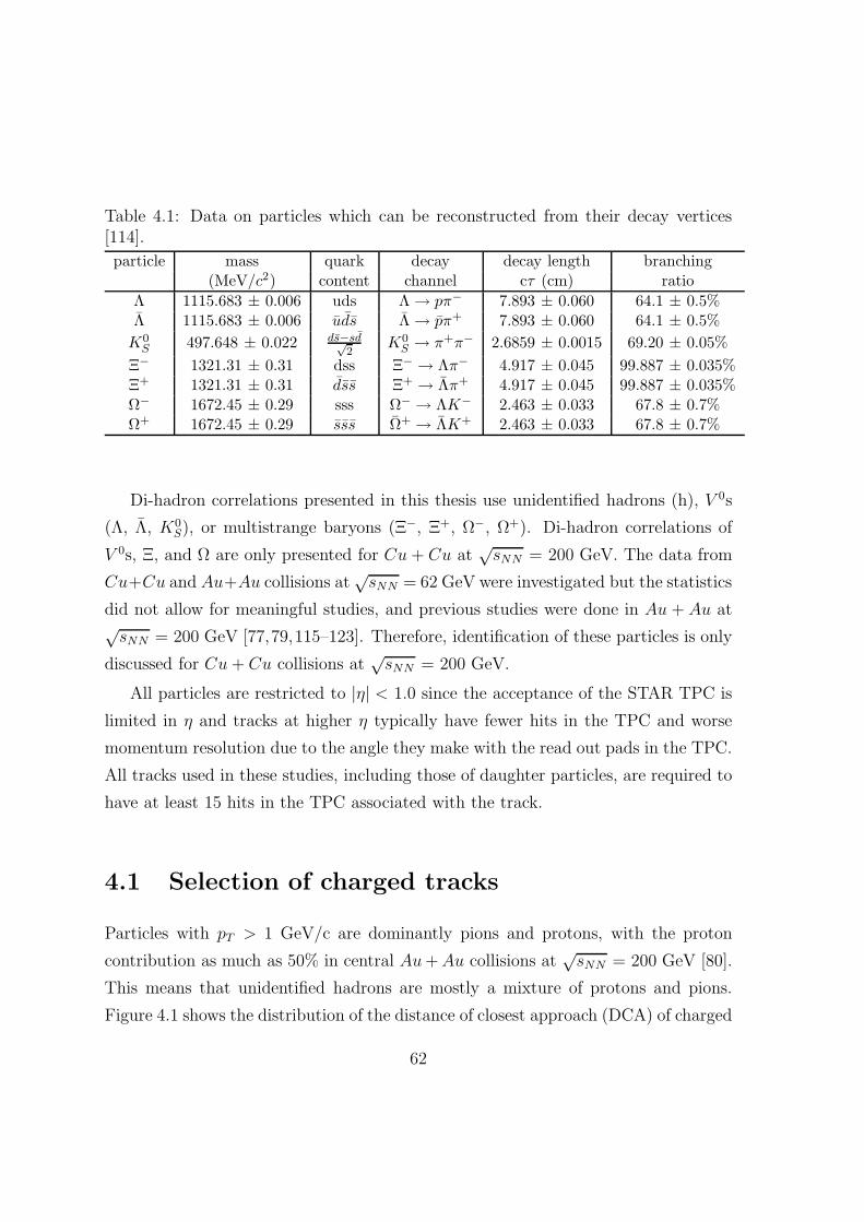
Table 4.1: Data on particles which can be reconstructed from their decay vertices[114].

particle mass quark decay decay length branching(MeV/c2) content channel cτ (cm) ratio

Λ 1115.683 ± 0.006 uds Λ → pπ− 7.893 ± 0.060 64.1 ± 0.5%Λ 1115.683 ± 0.006 uds Λ → pπ+ 7.893 ± 0.060 64.1 ± 0.5%

K0S 497.648 ± 0.022 ds−sd√

2K0

S → π+π− 2.6859 ± 0.0015 69.20 ± 0.05%

Ξ− 1321.31 ± 0.31 dss Ξ− → Λπ− 4.917 ± 0.045 99.887 ± 0.035%Ξ+ 1321.31 ± 0.31 dss Ξ+ → Λπ+ 4.917 ± 0.045 99.887 ± 0.035%Ω− 1672.45 ± 0.29 sss Ω− → ΛK− 2.463 ± 0.033 67.8 ± 0.7%Ω+ 1672.45 ± 0.29 sss Ω+ → ΛK+ 2.463 ± 0.033 67.8 ± 0.7%

Di-hadron correlations presented in this thesis use unidentified hadrons (h), V 0s

(Λ, Λ, K0S), or multistrange baryons (Ξ−, Ξ+, Ω−, Ω+). Di-hadron correlations of

V 0s, Ξ, and Ω are only presented for Cu+ Cu at√sNN = 200 GeV. The data from

Cu+Cu and Au+Au collisions at√sNN = 62 GeV were investigated but the statistics

did not allow for meaningful studies, and previous studies were done in Au + Au at√sNN = 200 GeV [77,79,115–123]. Therefore, identification of these particles is only

discussed for Cu+ Cu collisions at√sNN = 200 GeV.

All particles are restricted to |η| < 1.0 since the acceptance of the STAR TPC is

limited in η and tracks at higher η typically have fewer hits in the TPC and worse

momentum resolution due to the angle they make with the read out pads in the TPC.

All tracks used in these studies, including those of daughter particles, are required to

have at least 15 hits in the TPC associated with the track.

4.1 Selection of charged tracks

Particles with pT > 1 GeV/c are dominantly pions and protons, with the proton

contribution as much as 50% in central Au+Au collisions at√sNN = 200 GeV [80].

This means that unidentified hadrons are mostly a mixture of protons and pions.

Figure 4.1 shows the distribution of the distance of closest approach (DCA) of charged

62

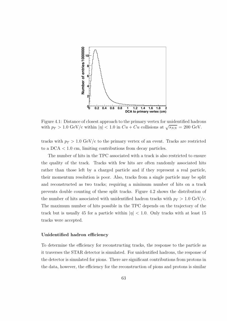
DCA to primary vertex (cm)0 0.2 0.4 0.6 0.8 1 1.2 1.4 1.6 1.8 2

Nu

mb

er

of

en

trie

s/1

00

00

00

0

2

4

6

8

10

Figure 4.1: Distance of closest approach to the primary vertex for unidentified hadronswith pT > 1.0 GeV/c within |η| < 1.0 in Cu+ Cu collisions at

√sNN = 200 GeV.

tracks with pT > 1.0 GeV/c to the primary vertex of an event. Tracks are restricted

to a DCA < 1.0 cm, limiting contributions from decay particles.

The number of hits in the TPC associated with a track is also restricted to ensure

the quality of the track. Tracks with few hits are often randomly associated hits

rather than those left by a charged particle and if they represent a real particle,

their momentum resolution is poor. Also, tracks from a single particle may be split

and reconstructed as two tracks; requiring a minimum number of hits on a track

prevents double counting of these split tracks. Figure 4.2 shows the distribution of

the number of hits associated with unidentified hadron tracks with pT > 1.0 GeV/c.

The maximum number of hits possible in the TPC depends on the trajectory of the

track but is usually 45 for a particle within |η| < 1.0. Only tracks with at least 15

tracks were accepted.

Unidentified hadron efficiency

To determine the efficiency for reconstructing tracks, the response to the particle as

it traverses the STAR detector is simulated. For unidentified hadrons, the response of

the detector is simulated for pions. There are significant contributions from protons in

the data, however, the efficiency for the reconstruction of pions and protons is similar

63

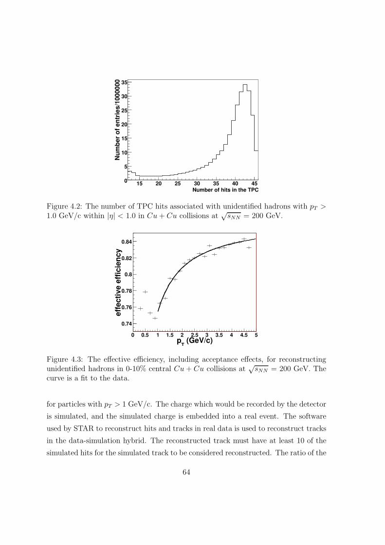
Number of hits in the TPC15 20 25 30 35 40 45

Nu

mb

er

of

en

trie

s/1

00

00

00

0

5

10

15

20

25

30

35

Figure 4.2: The number of TPC hits associated with unidentified hadrons with pT >1.0 GeV/c within |η| < 1.0 in Cu+ Cu collisions at

√sNN = 200 GeV.

(GeV/c)T

p0 0.5 1 1.5 2 2.5 3 3.5 4 4.5 5

eff

ecti

ve e

ffic

ien

cy

0.74

0.76

0.78

0.8

0.82

0.84

Figure 4.3: The effective efficiency, including acceptance effects, for reconstructingunidentified hadrons in 0-10% central Cu+ Cu collisions at

√sNN = 200 GeV. The

curve is a fit to the data.

for particles with pT > 1 GeV/c. The charge which would be recorded by the detector

is simulated, and the simulated charge is embedded into a real event. The software

used by STAR to reconstruct hits and tracks in real data is used to reconstruct tracks

in the data-simulation hybrid. The reconstructed track must have at least 10 of the

simulated hits for the simulated track to be considered reconstructed. The ratio of the

64

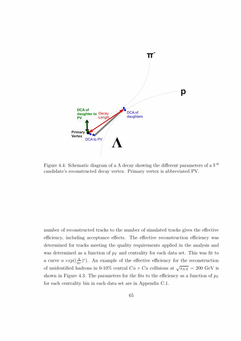
Figure 4.4: Schematic diagram of a Λ decay showing the different parameters of a V 0

candidate’s reconstructed decay vertex. Primary vertex is abbreviated PV.

number of reconstructed tracks to the number of simulated tracks gives the effective

efficiency, including acceptance effects. The effective reconstruction efficiency was

determined for tracks meeting the quality requirements applied in the analysis and

was determined as a function of pT and centrality for each data set. This was fit to

a curve a exp(( bpT

)c). An example of the effective efficiency for the reconstruction

of unidentified hadrons in 0-10% central Cu + Cu collisions at√sNN = 200 GeV is

shown in Figure 4.3. The parameters for the fits to the efficiency as a function of pT

for each centrality bin in each data set are in Appendix C.1.

65

4.2 V 0 reconstruction

A schematic diagram of the geometry of a Λ decay is shown in Figure 4.4. The K0S

decay is similar except for the identity of the daughters. This shows the different pa-

rameters describing the reconstructed decay vertex. Restrictions of these parameters

can be varied to alter the purity and the efficiency of reconstructed V 0 candidates.

To get a sample of V 0 candidates, all pairs of global tracks - those which are not

forced to go through the primary vertex - are combined. The invariant mass of the

track pair is calculated assuming that they are the decay daughters of a V 0. The

mass of a V 0 candidate is given by

mΛ =√

(mπ +mp)2 − (−→pπ− + −→pp)2

mΛ =√

(mπ +mp)2 − (−→pπ+ + −→pp)2 (4.1)

mK0S

=√

(mπ +mπ)2 − (−→pπ+ + −→pπ−)2

with the momentum given by

−→pΛ = −→pπ− + −→pp

−→pΛ = −→pπ+ + −→pp (4.2)

−−→pK0S

= −→pπ− + −→pπ+.

The combinatorial background in a heavy ion collision is considerably higher than

in e+ + e− or p+ p collisions, and is large for high particle multiplicities. This means

that the background is greater in central collisions than in peripheral collisions. The

background is dominated by primary tracks, or those which originate from the primary

vertex (PV). Some default cuts on track quality, daughter particle identification, and

geometry of the reconstructed vertex are applied to keep file sizes reasonable before

finer tuning of cuts. The list of default cuts is given in Table 4.2.

Figure 4.5 shows the DCA of the daughter tracks to each other and to the primary

vertex versus the invariant mass of the V 0 candidate. Plots with the parameter on the

y-axis and the mass of the candidate on the x-axis easily show the difference between

the signal and the background. The signal sits near the mass of the particles and has

66

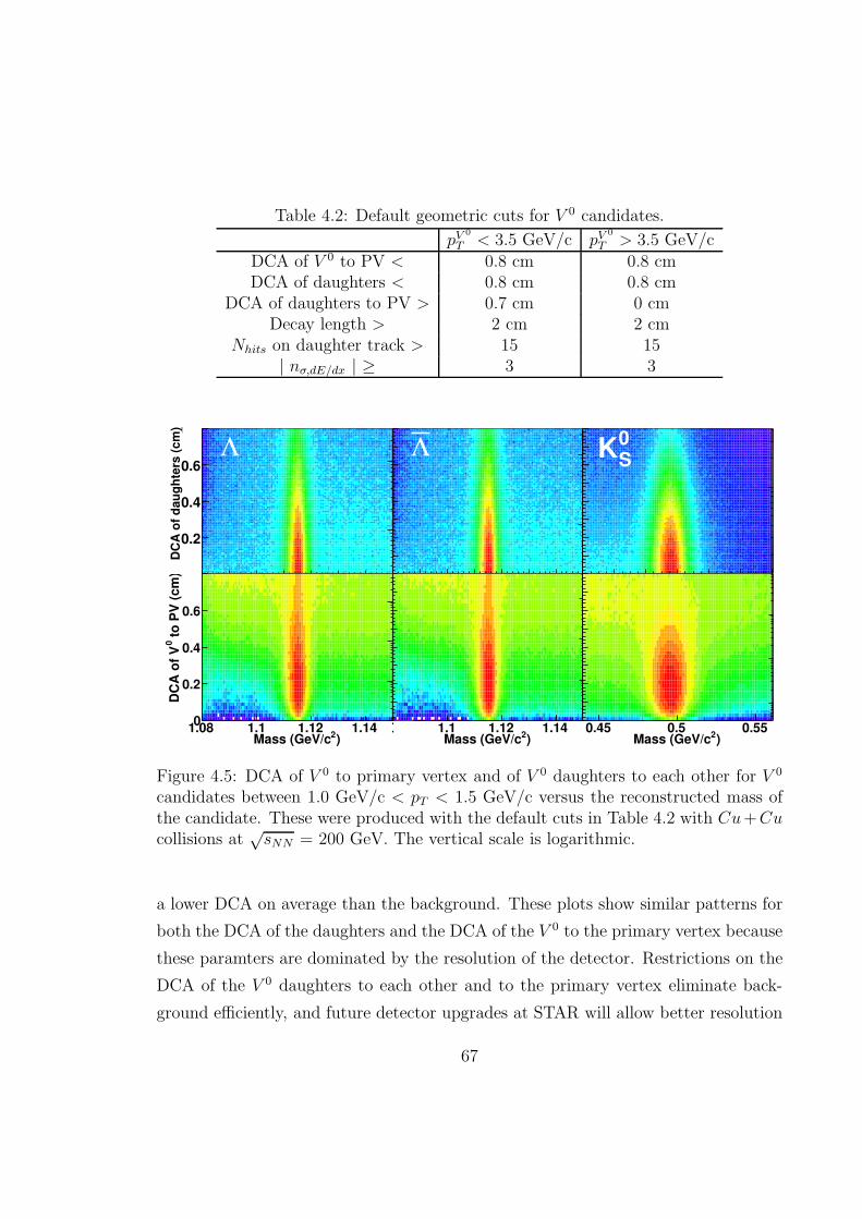
Table 4.2: Default geometric cuts for V 0 candidates.

pV 0

T < 3.5 GeV/c pV 0

T > 3.5 GeV/cDCA of V 0 to PV < 0.8 cm 0.8 cmDCA of daughters < 0.8 cm 0.8 cm

DCA of daughters to PV > 0.7 cm 0 cmDecay length > 2 cm 2 cm

Nhits on daughter track > 15 15| nσ,dE/dx | ≥ 3 3

1.08 1.09 1.1 1.11 1.12 1.13 1.14 1.15

DC

A o

f d

au

gh

ters

(c

m)

0

0.2

0.4

0.6

0.8

Λ

1.08 1.09 1.1 1.11 1.12 1.13 1.14 1.150

0.1

0.2

0.3

0.4

0.5

0.6

0.7

0.8

Λ

0.44 0.46 0.48 0.5 0.52 0.54 0.560

0.1

0.2

0.3

0.4

0.5

0.6

0.7

0.8

S0K

)2Mass (GeV/c1.08 1.1 1.12 1.14

to

PV

(c

m)

0D

CA

of

V

0

0.2

0.4

0.6

0.8

)2Mass (GeV/c1.08 1.1 1.12 1.140

0.1

0.2

0.3

0.4

0.5

0.6

0.7

0.8

)2Mass (GeV/c0.45 0.5 0.55

0

0.1

0.2

0.3

0.4

0.5

0.6

0.7

0.8

Figure 4.5: DCA of V 0 to primary vertex and of V 0 daughters to each other for V 0

candidates between 1.0 GeV/c < pT < 1.5 GeV/c versus the reconstructed mass ofthe candidate. These were produced with the default cuts in Table 4.2 with Cu+Cucollisions at

√sNN = 200 GeV. The vertical scale is logarithmic.

a lower DCA on average than the background. These plots show similar patterns for

both the DCA of the daughters and the DCA of the V 0 to the primary vertex because

these paramters are dominated by the resolution of the detector. Restrictions on the

DCA of the V 0 daughters to each other and to the primary vertex eliminate back-

ground efficiently, and future detector upgrades at STAR will allow better resolution

67

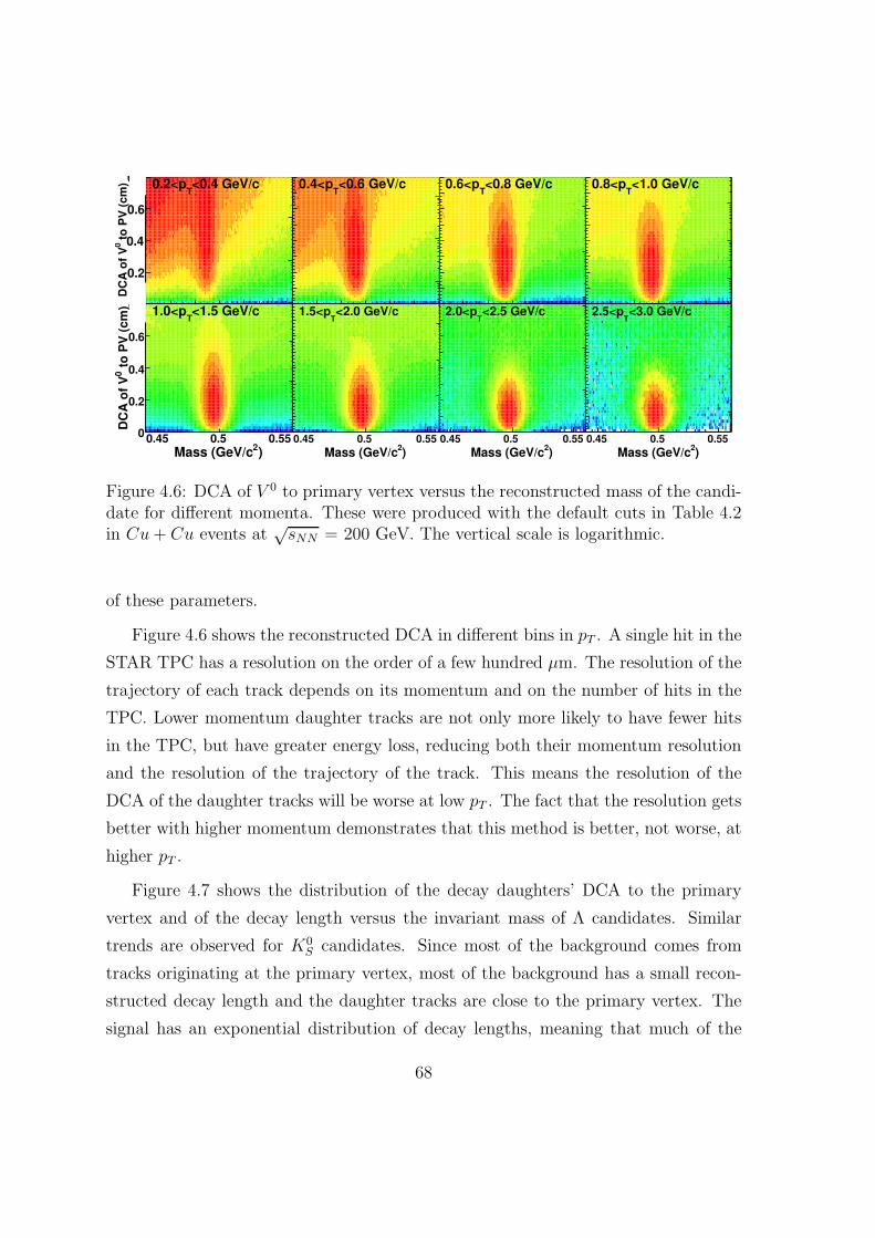
0.44 0.46 0.48 0.5 0.52 0.54 0.56

to

PV

(c

m)

0D

CA

of

V

0

0.2

0.4

0.6

0.8 <0.4 GeV/cT

0.2<p

0.44 0.46 0.48 0.5 0.52 0.54 0.560

0.1

0.2

0.3

0.4

0.5

0.6

0.7

0.8

<0.6 GeV/cT

0.4<p

0.44 0.46 0.48 0.5 0.52 0.54 0.560

0.1

0.2

0.3

0.4

0.5

0.6

0.7

0.8

<0.8 GeV/cT

0.6<p

0.44 0.46 0.48 0.5 0.52 0.54 0.560

0.1

0.2

0.3

0.4

0.5

0.6

0.7

0.8

<1.0 GeV/cT

0.8<p

)2Mass (GeV/c0.45 0.5 0.55

to

PV

(c

m)

0D

CA

of

V

0

0.2

0.4

0.6

0.8 <1.5 GeV/cT

1.0<p

)2

Mass (GeV/c0.45 0.5 0.55

0

0.1

0.2

0.3

0.4

0.5

0.6

0.7

0.8

<2.0 GeV/cT

1.5<p

)2

Mass (GeV/c0.45 0.5 0.55

0

0.1

0.2

0.3

0.4

0.5

0.6

0.7

0.8

<2.5 GeV/cT

2.0<p

)2

Mass (GeV/c0.45 0.5 0.55

0

0.1

0.2

0.3

0.4

0.5

0.6

0.7

0.8

<3.0 GeV/cT

2.5<p

Figure 4.6: DCA of V 0 to primary vertex versus the reconstructed mass of the candi-date for different momenta. These were produced with the default cuts in Table 4.2in Cu+ Cu events at

√sNN = 200 GeV. The vertical scale is logarithmic.

of these parameters.

Figure 4.6 shows the reconstructed DCA in different bins in pT . A single hit in the

STAR TPC has a resolution on the order of a few hundred µm. The resolution of the

trajectory of each track depends on its momentum and on the number of hits in the

TPC. Lower momentum daughter tracks are not only more likely to have fewer hits

in the TPC, but have greater energy loss, reducing both their momentum resolution

and the resolution of the trajectory of the track. This means the resolution of the

DCA of the daughter tracks will be worse at low pT . The fact that the resolution gets

better with higher momentum demonstrates that this method is better, not worse, at

higher pT .

Figure 4.7 shows the distribution of the decay daughters’ DCA to the primary

vertex and of the decay length versus the invariant mass of Λ candidates. Similar

trends are observed for K0S candidates. Since most of the background comes from

tracks originating at the primary vertex, most of the background has a small recon-

structed decay length and the daughter tracks are close to the primary vertex. The

signal has an exponential distribution of decay lengths, meaning that much of the

68

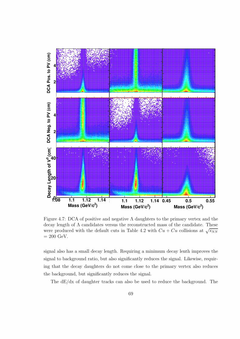
DC

A P

os. to

PV

(cm

)

0

2

4

6

0

1

2

3

4

5

6

0

500

1000

1500

2000

2500

3000

3500

4000

4500

0

1

2

3

4

5

6

1.08 1.09 1.1 1.11 1.12 1.13 1.14 1.15

DC

A N

eg

. to

PV

(cm

)

0

2

4

6

1.08 1.09 1.1 1.11 1.12 1.13 1.14 1.150

1

2

3

4

5

6

0

500

1000

1500

2000

2500

3000

3500

4000

4500

0.44 0.46 0.48 0.5 0.52 0.54 0.560

1

2

3

4

5

6

0

200

400

600

800

1000

1200

1400

1600

1800

2000

2200

)2Mass (GeV/c

1.08 1.1 1.12 1.14

(c

m)

0D

ec

ay

Le

ng

th o

f V

0

20

40

0

1000

2000

3000

4000

5000

)2Mass (GeV/c

1.08 1.1 1.12 1.140

5

10

15

20

25

30

35

40

45

50

0

1000

2000

3000

4000

5000

6000

)2Mass (GeV/c

0.45 0.5 0.550

5

10

15

20

25

30

35

40

45

50

Figure 4.7: DCA of positive and negative Λ daughters to the primary vertex and thedecay length of Λ candidates versus the reconstructed mass of the candidate. Thesewere produced with the default cuts in Table 4.2 with Cu + Cu collisions at

√sNN

= 200 GeV.

signal also has a small decay length. Requiring a minimum decay lenth improves the

signal to background ratio, but also significantly reduces the signal. Likewise, requir-

ing that the decay daughters do not come close to the primary vertex also reduces

the background, but significantly reduces the signal.

The dE/dx of daughter tracks can also be used to reduce the background. The

69

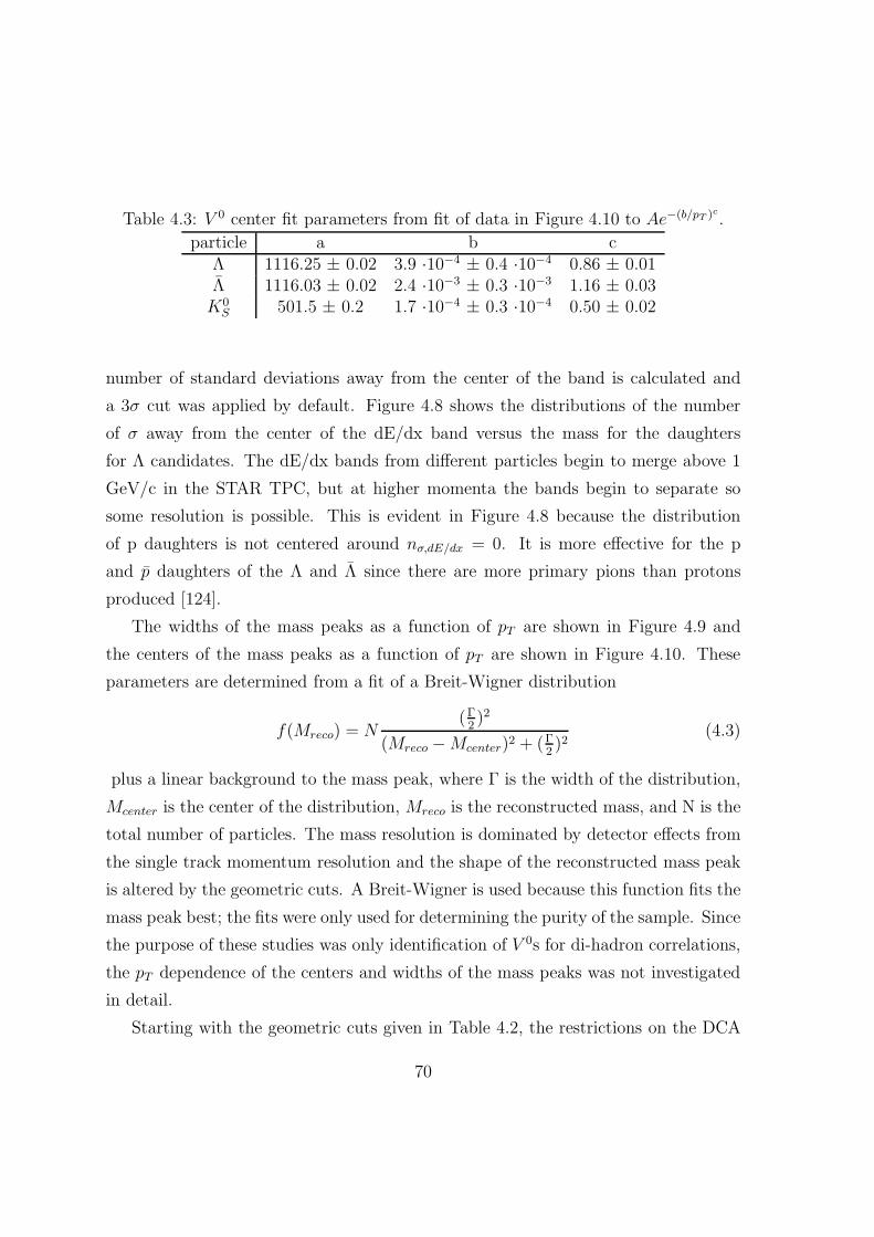
Table 4.3: V 0 center fit parameters from fit of data in Figure 4.10 to Ae−(b/pT )c

.

particle a b cΛ 1116.25 ± 0.02 3.9 ·10−4 ± 0.4 ·10−4 0.86 ± 0.01Λ 1116.03 ± 0.02 2.4 ·10−3 ± 0.3 ·10−3 1.16 ± 0.03K0

S 501.5 ± 0.2 1.7 ·10−4 ± 0.3 ·10−4 0.50 ± 0.02

number of standard deviations away from the center of the band is calculated and

a 3σ cut was applied by default. Figure 4.8 shows the distributions of the number

of σ away from the center of the dE/dx band versus the mass for the daughters

for Λ candidates. The dE/dx bands from different particles begin to merge above 1

GeV/c in the STAR TPC, but at higher momenta the bands begin to separate so

some resolution is possible. This is evident in Figure 4.8 because the distribution

of p daughters is not centered around nσ,dE/dx = 0. It is more effective for the p

and p daughters of the Λ and Λ since there are more primary pions than protons

produced [124].

The widths of the mass peaks as a function of pT are shown in Figure 4.9 and

the centers of the mass peaks as a function of pT are shown in Figure 4.10. These

parameters are determined from a fit of a Breit-Wigner distribution

f(Mreco) = N(Γ

2)2

(Mreco −Mcenter)2 + (Γ2)2

(4.3)

plus a linear background to the mass peak, where Γ is the width of the distribution,

Mcenter is the center of the distribution, Mreco is the reconstructed mass, and N is the

total number of particles. The mass resolution is dominated by detector effects from

the single track momentum resolution and the shape of the reconstructed mass peak

is altered by the geometric cuts. A Breit-Wigner is used because this function fits the

mass peak best; the fits were only used for determining the purity of the sample. Since

the purpose of these studies was only identification of V 0s for di-hadron correlations,

the pT dependence of the centers and widths of the mass peaks was not investigated

in detail.

Starting with the geometric cuts given in Table 4.2, the restrictions on the DCA

70

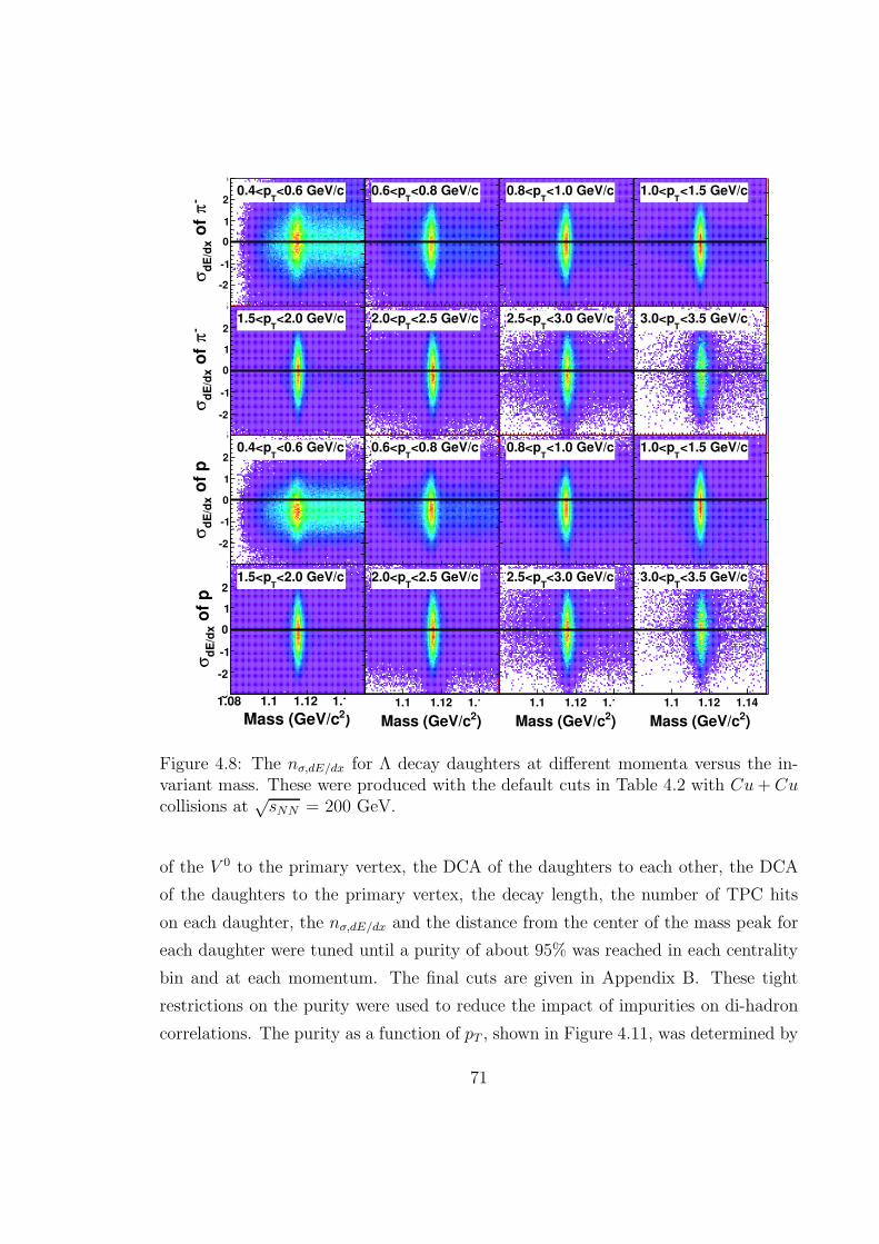
0

20

40

60

80

100

120

140

160

180

1.08 1.09 1.1 1.11 1.12 1.13 1.14 1.15

-π

of

dE

/dx

σ

-3

-2

-1

0

1

2

3

<0.6 GeV/cT

0.4<p

0

100

200

300

400

500

600

1.08 1.09 1.1 1.11 1.12 1.13 1.14 1.15-3

-2

-1

0

1

2

3

<0.8 GeV/cT

0.6<p

1.08 1.09 1.1 1.11 1.12 1.13 1.14 1.15-3

-2

-1

0

1

2

3

<1.0 GeV/cT

0.8<p

500

1000

1500

2000

2500

1.08 1.09 1.1 1.11 1.12 1.13 1.14 1.15-3

-2

-1

0

1

2

3

<1.5 GeV/cT

1.0<p

0

200

400

600

800

1000

1200

1400

1600

1800

-π

of

dE

/dx

σ

-3

-2

-1

0

1

2

3

<2.0 GeV/cT

1.5<p

0

100

200

300

400

500

600

-3

-2

-1

0

1

2

3

<2.5 GeV/cT

2.0<p

-3

-2

-1

0

1

2

3

<3.0 GeV/cT

2.5<p

0

10

20

30

40

50

60

70

-3

-2

-1

0

1

2

3

<3.5 GeV/cT

3.0<p

0

20

40

60

80

100

120

140

160

180

200

220

240

1.08 1.09 1.1 1.11 1.12 1.13 1.14 1.15

of

pd

E/d

xσ

-3

-2

-1

0

1

2

3

<0.6 GeV/cT

0.4<p

0

100

200

300

400

500

600

700

1.08 1.09 1.1 1.11 1.12 1.13 1.14 1.15-3

-2

-1

0

1

2

3

<0.8 GeV/cT

0.6<p

1.08 1.09 1.1 1.11 1.12 1.13 1.14 1.15-3

-2

-1

0

1

2

3

<1.0 GeV/cT

0.8<p

0

500

1000

1500

2000

2500

1.08 1.09 1.1 1.11 1.12 1.13 1.14 1.15-3

-2

-1

0

1

2

3

<1.5 GeV/cT

1.0<p

0

200

400

600

800

1000

1200

1400

1600

)2Mass (GeV/c1.08 1.1 1.12 1.14

of

pd

E/d

xσ

-3

-2

-1

0

1

2

3<2.0 GeV/c

T1.5<p

0

100

200

300

400

500

600

)2Mass (GeV/c

1.08 1.1 1.12 1.14-3

-2

-1

0

1

2

3

<2.5 GeV/cT

2.0<p

0

20

40

60

80

100

120

140

160

180

)2Mass (GeV/c

1.08 1.1 1.12 1.14-3

-2

-1

0

1

2

3

<3.0 GeV/cT

2.5<p

0

10

20

30

40

50

)2Mass (GeV/c

1.08 1.1 1.12 1.14-3

-2

-1

0

1

2

3

<3.5 GeV/cT

3.0<p

Figure 4.8: The nσ,dE/dx for Λ decay daughters at different momenta versus the in-variant mass. These were produced with the default cuts in Table 4.2 with Cu+ Cucollisions at

√sNN = 200 GeV.

of the V 0 to the primary vertex, the DCA of the daughters to each other, the DCA

of the daughters to the primary vertex, the decay length, the number of TPC hits

on each daughter, the nσ,dE/dx and the distance from the center of the mass peak for

each daughter were tuned until a purity of about 95% was reached in each centrality

bin and at each momentum. The final cuts are given in Appendix B. These tight

restrictions on the purity were used to reduce the impact of impurities on di-hadron

correlations. The purity as a function of pT , shown in Figure 4.11, was determined by

71

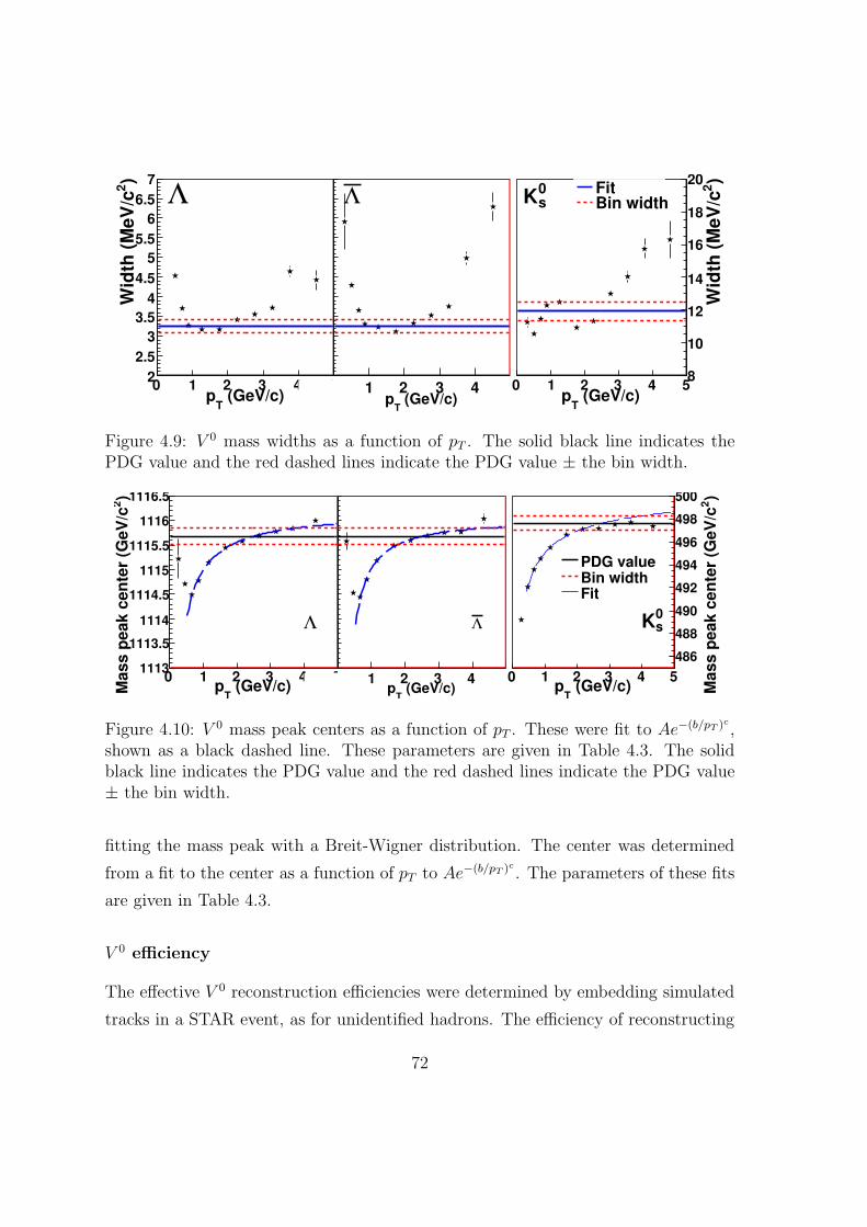
(GeV/c)T

p0 1 2 3 4 5

)2

Wid

th (

MeV

/c

2

2.5

3

3.5

4

4.5

5

5.5

6

6.5

7

Λ

(GeV/c)T

p0 1 2 3 4 52

2.5

3

3.5

4

4.5

5

5.5

6

6.5

7

Λ

(GeV/c)T

p0 1 2 3 4 5

)2

Wid

th (

MeV

/c

8

10

12

14

16

18

20

s0

KFitBin width

Figure 4.9: V 0 mass widths as a function of pT . The solid black line indicates thePDG value and the red dashed lines indicate the PDG value ± the bin width.

(GeV/c)T

p0 1 2 3 4 5

)2

Ma

ss

pe

ak

ce

nte

r (G

eV

/c

1113

1113.5

1114

1114.5

1115

1115.5

1116

1116.5

Λ

(GeV/c)T

p0 1 2 3 4 5

1113

1113.5

1114

1114.5

1115

1115.5

1116

1116.5

Λ

(GeV/c)T

p0 1 2 3 4 5

)2

Ma

ss

pe

ak

ce

nte

r (G

eV

/c

486

488

490

492

494

496

498

500

PDG valueBin widthFit

s0

K

Figure 4.10: V 0 mass peak centers as a function of pT . These were fit to Ae−(b/pT )c

,shown as a black dashed line. These parameters are given in Table 4.3. The solidblack line indicates the PDG value and the red dashed lines indicate the PDG value± the bin width.

fitting the mass peak with a Breit-Wigner distribution. The center was determined

from a fit to the center as a function of pT to Ae−(b/pT )c

. The parameters of these fits

are given in Table 4.3.

V 0 efficiency

The effective V 0 reconstruction efficiencies were determined by embedding simulated

tracks in a STAR event, as for unidentified hadrons. The efficiency of reconstructing

72

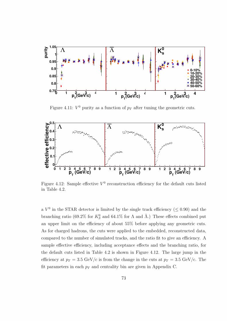
(GeV/c)T

p0 1 2 3 4 5

pu

rity

0.75

0.8

0.85

0.9

0.95

1

1.05Λ

(GeV/c)T

p0 1 2 3 4 5

0.75

0.8

0.85

0.9

0.95

1

1.05

Λ

(GeV/c)T

p0 1 2 3 4 5

0.75

0.8

0.85

0.9

0.95

1

1.05

s0

K

0-10%10-20%20-30%30-40%40-50%50-60%

Figure 4.11: V 0 purity as a function of pT after tuning the geometric cuts.

(GeV/c)T

p0 1 2 3 4 5 6 7 8 9 10

eff

ecti

ve e

ffic

ien

cy

0

0.1

0.2

0.3

0.4

0.5

Λ

(GeV/c)T

p0 1 2 3 4 5 6 7 8 9 10

0

0.1

0.2

0.3

0.4

0.5

Λ

(GeV/c)T

p0 1 2 3 4 5 6 7 8 9 10

0

0.1

0.2

0.3

0.4

0.5

s0

K

Figure 4.12: Sample effective V 0 reconstruction efficiency for the default cuts listedin Table 4.2.

a V 0 in the STAR detector is limited by the single track efficiency (≤ 0.90) and the

branching ratio (69.2% for K0S and 64.1% for Λ and Λ.) These effects combined put

an upper limit on the efficiency of about 55% before applying any geometric cuts.

As for charged hadrons, the cuts were applied to the embedded, reconstructed data,

compared to the number of simulated tracks, and the ratio fit to give an efficiency. A

sample effective efficiency, including acceptance effects and the branching ratio, for

the default cuts listed in Table 4.2 is shown in Figure 4.12. The large jump in the

efficiency at pT = 3.5 GeV/c is from the change in the cuts at pT = 3.5 GeV/c. The

fit parameters in each pT and centrality bin are given in Appendix C.

73

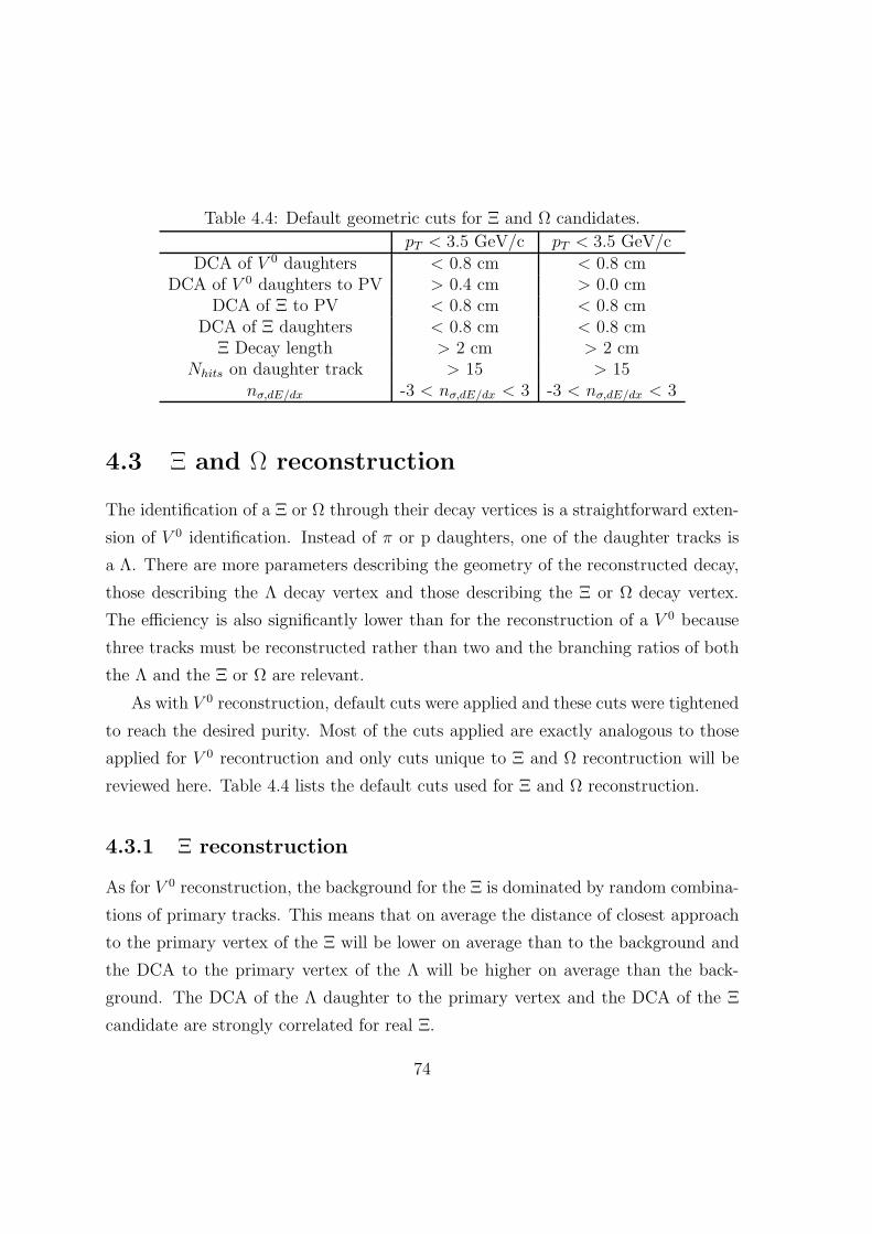
Table 4.4: Default geometric cuts for Ξ and Ω candidates.

pT < 3.5 GeV/c pT < 3.5 GeV/cDCA of V 0 daughters < 0.8 cm < 0.8 cm

DCA of V 0 daughters to PV > 0.4 cm > 0.0 cmDCA of Ξ to PV < 0.8 cm < 0.8 cm

DCA of Ξ daughters < 0.8 cm < 0.8 cmΞ Decay length > 2 cm > 2 cm

Nhits on daughter track > 15 > 15nσ,dE/dx -3 < nσ,dE/dx < 3 -3 < nσ,dE/dx < 3

4.3 Ξ and Ω reconstruction

The identification of a Ξ or Ω through their decay vertices is a straightforward exten-

sion of V 0 identification. Instead of π or p daughters, one of the daughter tracks is

a Λ. There are more parameters describing the geometry of the reconstructed decay,

those describing the Λ decay vertex and those describing the Ξ or Ω decay vertex.

The efficiency is also significantly lower than for the reconstruction of a V 0 because

three tracks must be reconstructed rather than two and the branching ratios of both

the Λ and the Ξ or Ω are relevant.

As with V 0 reconstruction, default cuts were applied and these cuts were tightened

to reach the desired purity. Most of the cuts applied are exactly analogous to those

applied for V 0 recontruction and only cuts unique to Ξ and Ω recontruction will be

reviewed here. Table 4.4 lists the default cuts used for Ξ and Ω reconstruction.

4.3.1 Ξ reconstruction

As for V 0 reconstruction, the background for the Ξ is dominated by random combina-

tions of primary tracks. This means that on average the distance of closest approach

to the primary vertex of the Ξ will be lower on average than to the background and

the DCA to the primary vertex of the Λ will be higher on average than the back-

ground. The DCA of the Λ daughter to the primary vertex and the DCA of the Ξ

candidate are strongly correlated for real Ξ.

74

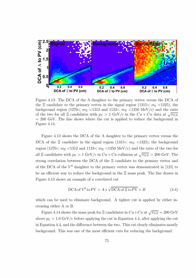
Figure 4.13: The DCA of the Λ daughter to the primary vertex versus the DCA ofthe Ξ candidate to the primary vertex in the signal region (1315< mξ <1325), thebackground region (1270< mΞ <1312 and 1133< mΞ <1350 MeV/c) and the ratioof the two for all Ξ candidates with pT > 1 GeV/c in the Cu + Cu data at

√sNN

= 200 GeV. The line shows where the cut is applied to reduce the background inFigure 4.14.

Figure 4.13 shows the DCA of the Λ daughter to the primary vertex versus the

DCA of the Ξ candidate in the signal region (1315< mΞ <1325), the background

region (1270< mΞ <1312 and 1133< mΞ <1350 MeV/c) and the ratio of the two for

all Ξ candidates with pT > 1 GeV/c in Cu+Cu collisions at√sNN = 200 GeV. The

strong correlation between the DCA of the Ξ candidate to the primary vertex and

of the DCA of the V 0 daughter to the primary vertex was demonstrated in [125] to

be an efficient way to reduce the background in the Ξ mass peak. The line drawn in

Figure 4.13 shows an example of a correlated cut

DCAof V0 toPV > A ∗√

DCAof Ξ toPV +B (4.4)

which can be used to eliminate background. A tighter cut is applied by either in-

creasing either A or B.

Figure 4.14 shows the mass peak for Ξ candidates in Cu+Cu at√sNN = 200 GeV

above pT > 1.0 GeV/c before applying the cut in Equation 4.4, after applying the cut

in Equation 4.4, and the difference between the two. This cut clearly eliminates mostly

background. This was one of the most efficient cuts for reducing the background.

75

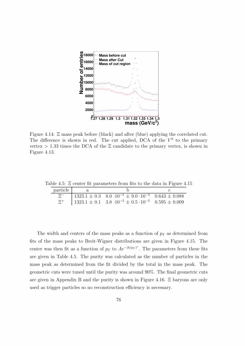
)2mass (GeV/c1.27 1.28 1.29 1.3 1.31 1.32 1.33 1.34 1.35

Nu

mb

er

of

en

trie

s

0

2000

4000

6000

8000

10000

12000

14000

16000

18000 Mass before cut

Mass after CutMass of cut region

Figure 4.14: Ξ mass peak before (black) and after (blue) applying the correlated cut.The difference is shown in red. The cut applied, DCA of the V 0 to the primaryvertex > 1.33 times the DCA of the Ξ candidate to the primary vertex, is shown inFigure 4.13.

Table 4.5: Ξ center fit parameters from fits to the data in Figure 4.15

particle a b cΞ− 1323.1 ± 0.3 8.0 ·10−5 ± 9.0 ·10−5 0.643 ± 0.088Ξ+ 1323.1 ± 0.1 3.8 ·10−5 ± 0.5 ·10−5 0.595 ± 0.009

The width and centers of the mass peaks as a function of pT as determined from

fits of the mass peaks to Breit-Wigner distributions are given in Figure 4.15. The

center was then fit as a function of pT to Ae−(b/pT )c

. The parameters from these fits

are given in Table 4.5. The purity was calculated as the number of particles in the

mass peak as determined from the fit divided by the total in the mass peak. The

geometric cuts were tuned until the purity was around 90%. The final geometric cuts

are given in Appendix B and the purity is shown in Figure 4.16. Ξ baryons are only

used as trigger particles so no reconstruction efficiency is necessary.

76

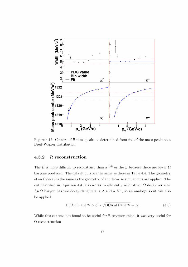
0 0.5 1 1.5 2 2.5 3 3.5 4 4.5 5

)2

Wid

th (

Me

V/c

0

1

2

3

4

5

6

7

8

9

-Ξ

PDG valueBin widthFit

0 0.5 1 1.5 2 2.5 3 3.5 4 4.5 50

1

2

3

4

5

6

7

8

9

+Ξ

(GeV/c)T

p0 1 2 3 4 5

)2

Ma

ss

pe

ak

ce

nte

r (M

eV

/c

1318

1319

1320

1321

1322

-Ξ

(GeV/c)T

p0 1 2 3 4 5

1318

1318.5

1319

1319.5

1320

1320.5

1321

1321.5

1322

1322.5

+Ξ

Figure 4.15: Centers of Ξ mass peaks as determined from fits of the mass peaks to aBreit-Wigner distribution

4.3.2 Ω reconstruction

The Ω is more difficult to reconstruct than a V 0 or the Ξ because there are fewer Ω

baryons produced. The default cuts are the same as those in Table 4.4. The geometry

of an Ω decay is the same as the geometry of a Ξ decay so similar cuts are applied. The

cut described in Equation 4.4, also works to efficiently reconstruct Ω decay vertices.

An Ω baryon has two decay daughters, a Λ and a K−, so an analogous cut can also

be applied:

DCAof π toPV > C ∗√

DCA of Ω to PV +D. (4.5)

While this cut was not found to be useful for Ξ reconstruction, it was very useful for

Ω reconstruction.

77

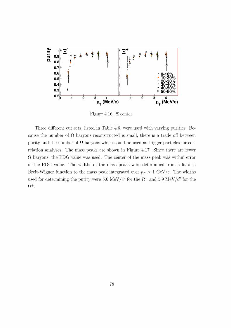
(MeV/c)T

p0 1 2 3 4 5

pu

rity

0.2

0.3

0.4

0.5

0.6

0.7

0.8

0.9

1-

Ξ

(MeV/c)T

p0 1 2 3 4 5

0.2

0.3

0.4

0.5

0.6

0.7

0.8

0.9

1

0-10%10-20%20-30%30-40%40-50%50-60%

+Ξ

Figure 4.16: Ξ center

Three different cut sets, listed in Table 4.6, were used with varying purities. Be-

cause the number of Ω baryons reconstructed is small, there is a trade off between

purity and the number of Ω baryons which could be used as trigger particles for cor-

relation analyses. The mass peaks are shown in Figure 4.17. Since there are fewer

Ω baryons, the PDG value was used. The center of the mass peak was within error

of the PDG value. The widths of the mass peaks were determined from a fit of a

Breit-Wigner function to the mass peak integrated over pT > 1 GeV/c. The widths

used for determining the purity were 5.6 MeV/c2 for the Ω− and 5.9 MeV/c2 for the

Ω+.

78

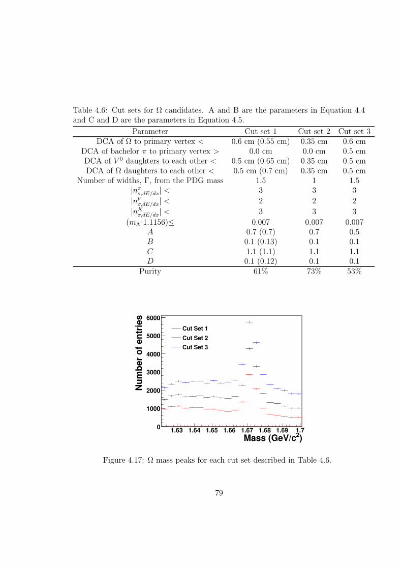
Table 4.6: Cut sets for Ω candidates. A and B are the parameters in Equation 4.4and C and D are the parameters in Equation 4.5.

Parameter Cut set 1 Cut set 2 Cut set 3DCA of Ω to primary vertex < 0.6 cm (0.55 cm) 0.35 cm 0.6 cm

DCA of bachelor π to primary vertex > 0.0 cm 0.0 cm 0.5 cmDCA of V 0 daughters to each other < 0.5 cm (0.65 cm) 0.35 cm 0.5 cmDCA of Ω daughters to each other < 0.5 cm (0.7 cm) 0.35 cm 0.5 cm

Number of widths, Γ, from the PDG mass 1.5 1 1.5|nπ

σ,dE/dx| < 3 3 3

|npσ,dE/dx| < 2 2 2

|nKσ,dE/dx| < 3 3 3

(mΛ-1.1156)≤ 0.007 0.007 0.007A 0.7 (0.7) 0.7 0.5B 0.1 (0.13) 0.1 0.1C 1.1 (1.1) 1.1 1.1D 0.1 (0.12) 0.1 0.1

Purity 61% 73% 53%

)2Mass (GeV/c1.63 1.64 1.65 1.66 1.67 1.68 1.69 1.7

Nu

mb

er

of

en

trie

s

0

1000

2000

3000

4000

5000

6000

Cut Set 1

Cut Set 2

Cut Set 3

Figure 4.17: Ω mass peaks for each cut set described in Table 4.6.

79

80

Chapter 5

Correlation Method

5.1 Event selection

Data in this thesis are from Au + Au collisions at√sNN = 62 GeV from RHIC’s

fourth run (2004) and Cu+Cu collisions at√sNN = 62 GeV and

√sNN = 200 GeV

from RHIC’s fifth run (2005.) These data are compared to previous studies done in

Au + Au collisions at√sNN = 200 GeV from RHIC’s fourth year run. In order to

be usable for analyses, events must have a clearly defined vertex. For all systems

and energies, the vertex is limited to within 30 cm of the center of the TPC along

the beam axis. The further an event is from the center of the TPC the lower the

geometric acceptance; a 30 cm cut allows reasonably uniform geometric acceptance.

The impact parameter of events cannot be directly measured, so instead the cen-

trality of the collision is given as a percentage of events in a sample. These percentages

are determined by dividing the event sample into percentages of centrality as deter-

mined by the reference multiplicity1. This is compared to the distribution of impact

parameters expected in a Glauber Monte Carlo model [41] so that the 0-10% central

events roughly corresponds to the highest 10% of impact parameters. The Glauber

model assumes a realistic distribution of nucleons in nuclei, such as a Woods-Saxon

density profile, and samples collisions with a uniform impact parameter, b, ranging

1The reference multiplicity is defined as the uncorrected number of tracks in the TPC within|η| < 0.5.

81

between 0 and a cut-off bmax. Based on the assumption that nucleons travel in a

straight line as the nuclei interact and that nucleons interact with the same cross sec-

tion as protons, the number of nuclei which participate in the collision at least once

(Npart) and the total number of nucleon-nucleon collisions (Nbin) is calculated. Npart

is bounded by the sum of the nucleons in the colliding nuclei and Nbin is bounded by

the product of the number of nucleons in the two nuclei. Soft particle production is

expected to scale with Npart and hard particle production, such as that from jets, is

expected to scale with Nbin. Details of Glauber Monte Carlo models and how they are

used in heavy ion collisions can be found in [41]. The Glauber model is compared to

the data to determine the centrality of an event from its reference multiplicity. The

centrality bins used in this analysis and their corresponding reference multiplicities,

Nbin, and Npart are given in Appendix D.

Events from Au + Au collisions have a more clearly defined vertex because there

are more tracks produced in an Au+Au collision which can be used to reconstruct the

vertex position. The 80% most central events were usable in Au+Au collisions. Fewer

tracks are produced in Cu+Cu collisions and the luminosity was significantly higher

in 2005 than in 2006. The higher luminosity meant that particles from a previous

event could still be traversing the TPC when a new event triggered the detector to

begin reading out data, a problem called pile-up. For higher multiplicities, it is still

possible to determine the primary vertex, but the lower the multiplicity the harder it

is to determine where the vertex from the event which triggered the detector is. For

this reason only the 60% most central data from these events was usable. For more

peripheral events, the vertex which triggered the event could not be found in more

than 2% of events, in large part because vertices from pile-up events usually had a

greater multipicity. Full details of the separation of the vertices from the triggered

event and from pile-up events can be found in [126].

5.2 Correlation technique

In a given event, a high-pT track, called the trigger particle, is selected and the dis-

tribution of all lower momentum particles, called associated particles, relative to that

82

track in ∆η and ∆φ is determined. Tracks are selected as described in Chapter 4, with

no additional restrictions on the high momentum track other than the pT . Multiple

tracks in a single event may be counted as trigger particles. The data are symmet-

ric about ∆φ = 0 and ∆η = 0 because the sign of ∆φ and ∆η are determined by

an arbitrary choice of coordinates. Since many of these measurements are limited

by statistics, the data are reflected about ∆φ = 0 and ∆η = 0 to minimize statis-

tical fluctuations. The single track efficiency, described in Chapter 4, is dependent

on particle type, collision system and energy, pT , and centrality and the correction

for associated particles is applied on a track-by-track basis. The final distribution is

normalized by the number of trigger particles, so no correction for the efficiency of

reconstructing the trigger particle is necessary. Two corrections for the acceptance

of track pairs in ∆φ and ∆η, described below, are applied. This is done for the full

sample of events to give the average distribution of associated particles relative to a

high-pT trigger particle 1Ntrigger

d2Nd∆φd∆η

.

Two key features of the STAR TPC affect the geometric acceptance of track

pairs. Tracks in the TPC can only be resolved well for -1 < η < 1 because the lower

geometric acceptance leads to tracks with fewer hits in the TPC, so only tracks within

-1 < η < 1 are used for this analysis. Track pairs with ∆η ≈ 0 are nearly always

accepted, however, track pairs with |∆η | ≈ 2 are only accepted if the tracks are near

opposite edges of the detector. Therefore acceptance is roughly 100% near ∆η ≈ 0

but roughly 0% near |∆η | ≈ 2. This leads to an acceptance in ∆η with a triangular

shape.

In addition, as discussed in Chapter 3, there are gaps between each of the 12 TPC

sectors. This leads to holes in the acceptance in azimuth. Most tracks will have hits

in multiple sectors, however, the loss of hits leads to a decrease in the reconstruction

efficiency for tracks at the angles of the sector boundaries. A sample distribution of

tracks reconstructed in the TPC is shown in Figure 5.1 showing the lower efficiency

at the TPC sector boundaries.

To correct for these effects, the distributions of tracks for both the associated

and the trigger particles are recorded. A random trigger (φ,η) is chosen from this

83

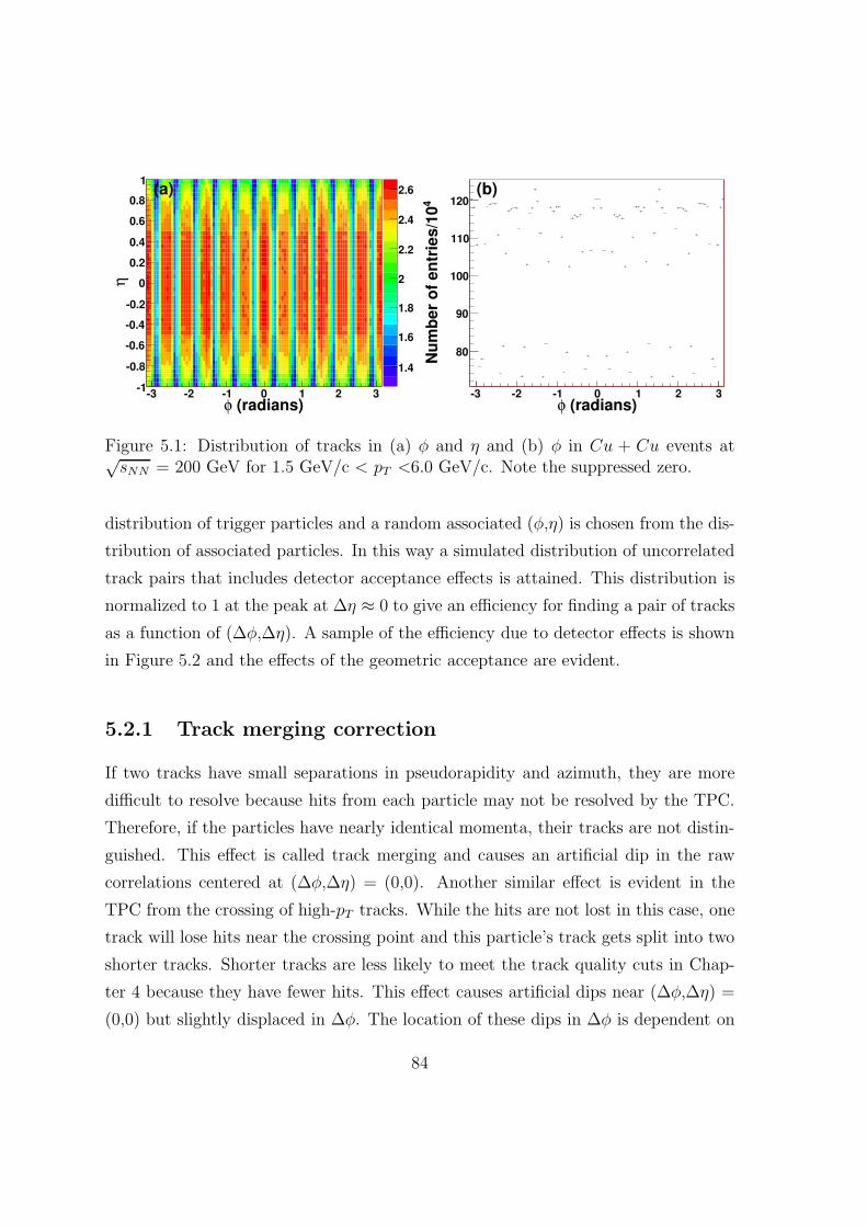
1.4

1.6

1.8

2

2.2

2.4

2.6

(radians)φ-3 -2 -1 0 1 2 3

η

-1

-0.8

-0.6

-0.4

-0.2

0

0.2

0.4

0.6

0.8

1(a)

(radians)φ-3 -2 -1 0 1 2 3

4N

um

be

r o

f e

ntr

ies

/10

80

90

100

110

120(b)

Figure 5.1: Distribution of tracks in (a) φ and η and (b) φ in Cu + Cu events at√sNN = 200 GeV for 1.5 GeV/c < pT <6.0 GeV/c. Note the suppressed zero.

distribution of trigger particles and a random associated (φ,η) is chosen from the dis-

tribution of associated particles. In this way a simulated distribution of uncorrelated

track pairs that includes detector acceptance effects is attained. This distribution is

normalized to 1 at the peak at ∆η ≈ 0 to give an efficiency for finding a pair of tracks

as a function of (∆φ,∆η). A sample of the efficiency due to detector effects is shown

in Figure 5.2 and the effects of the geometric acceptance are evident.

5.2.1 Track merging correction

If two tracks have small separations in pseudorapidity and azimuth, they are more

difficult to resolve because hits from each particle may not be resolved by the TPC.

Therefore, if the particles have nearly identical momenta, their tracks are not distin-

guished. This effect is called track merging and causes an artificial dip in the raw

correlations centered at (∆φ,∆η) = (0,0). Another similar effect is evident in the

TPC from the crossing of high-pT tracks. While the hits are not lost in this case, one

track will lose hits near the crossing point and this particle’s track gets split into two

shorter tracks. Shorter tracks are less likely to meet the track quality cuts in Chap-

ter 4 because they have fewer hits. This effect causes artificial dips near (∆φ,∆η) =

(0,0) but slightly displaced in ∆φ. The location of these dips in ∆φ is dependent on

84

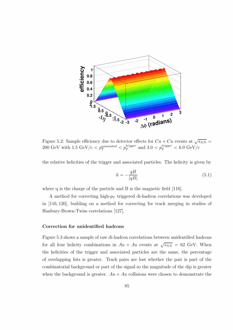
(radians)φ∆

-3 -2 -1 0 1 2 3

η∆-2

-1.5-1

-0.50

0.511.52

eff

icie

nc

y

0

0.2

0.4

0.6

0.8

1

Figure 5.2: Sample efficiency due to detector effects for Cu+ Cu events at√sNN =

200 GeV with 1.5 GeV/c < passociatedT < ptrigger

T and 3.0 < ptriggerT < 6.0 GeV/c

the relative helicities of the trigger and associated particles. The helicity is given by

h = − qB

|qB| (5.1)

where q is the charge of the particle and B is the magnetic field [116].

A method for correcting high-pT triggered di-hadron correlations was developed

in [116, 120], building on a method for correcting for track merging in studies of

Hanbury-Brown-Twiss correlations [127].

Correction for unidentified hadrons

Figure 5.3 shows a sample of raw di-hadron correlations between unidentified hadrons

for all four helicity combinations in Au + Au events at√sNN = 62 GeV. When

the helicities of the trigger and associated particles are the same, the percentage

of overlapping hits is greater. Track pairs are lost whether the pair is part of the

combinatorial background or part of the signal so the magnitude of the dip is greater

when the background is greater. Au+ Au collisions were chosen to demonstrate the

85

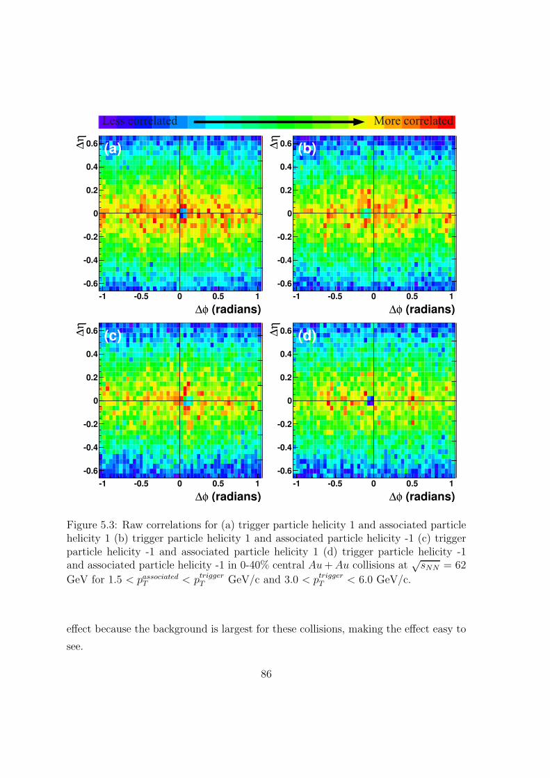
0.008

0.009

0.01

0.011

0.012

(radians)φ∆

-1 -0.5 0 0.5 1

η∆

-0.6

-0.4

-0.2

0

0.2

0.4

0.6 (a)

0.009

0.01

0.011

0.012

0.013

0.014

0.015

(radians)φ∆

-1 -0.5 0 0.5 1

η∆

-0.6

-0.4

-0.2

0

0.2

0.4

0.6 (b)

0.008

0.009

0.01

0.011

0.012

0.013

(radians)φ∆

-1 -0.5 0 0.5 1

η∆

-0.6

-0.4

-0.2

0

0.2

0.4

0.6 (c)

0.009

0.01

0.011

0.012

0.013

0.014

0.015

(radians)φ∆

-1 -0.5 0 0.5 1

η∆

-0.6

-0.4

-0.2

0

0.2

0.4

0.6 (d)

Figure 5.3: Raw correlations for (a) trigger particle helicity 1 and associated particlehelicity 1 (b) trigger particle helicity 1 and associated particle helicity -1 (c) triggerparticle helicity -1 and associated particle helicity 1 (d) trigger particle helicity -1and associated particle helicity -1 in 0-40% central Au+Au collisions at

√sNN = 62

GeV for 1.5 < passociatedT < ptrigger

T GeV/c and 3.0 < ptriggerT < 6.0 GeV/c.

effect because the background is largest for these collisions, making the effect easy to

see.

86

The number of hits shared by two tracks is calculated based on the trajectory of

the track and if more than 10% of hits are shared between two tracks, the tracks are

considered merged and the track pair is discarded. To get an acceptance correction

for this effect, the trigger particle is mixed with associated particles from another

event. This procedure is called event mixing. The trigger and associated particles

from separate events will have no real correlations so any structures in the resulting

(∆φ,∆η) distribution will result only from detector acceptance effects, including track

merging. In the mixed events, the origin of the associated track must be shifted to

the new vertex so that the percentage of merged hits can be calculated accurately. In

addition, mixed events are required to have vertices within 2 cm of each other along

the beam axis in order to ensure similar geometric acceptance in both events. The

reference multiplicities of both events are required to be within 10. The calculation

of the number of hits which may be shared by the tracks does not describe the

performance of the TPC perfectly and some track pairs which were calculated to

share more than 10% of their hits are reconstructed. These pairs are discarded even

if they were reconstructed so that the percentage of merged track pairs is the same

in the data and the mixed events. The mixed events are then used to determine an

acceptance correction as a function of ∆φ and ∆η for track pairs. Most of the dip is

corrected away when the data are divided by the efficiency from mixed events [116,

120]. While the method discused in Section 5.2 corrects for the geometric acceptance

of the detector, this method corrects for both the geometric acceptance and for track

merging. This method is much more CPU-intensive and therefore was only applied

for small (∆φ,∆η).

Figure 5.4(a) shows the data and Figure 5.4(b) shows the mixed events for a

sample correlation. The dip has a different shape when the helicities of the tracks are

the same and when they are opposite. To do the correction the data and mixed events

are rotated so that the dip is in the same location. The same helicity data are divided

by the acceptance correction from the same helicity events and the opposite helicity

data are divided by the acceptance correction from the opposite helicity mixed events.

These data are then added after the acceptance correction. A small residual dip

remains because mixed events to do not recreate the dip perfectly. The remaining dip

87

is corrected for using the symmetry of the correlations. Since the data are symmetric

about ∆φ = 0, the data on the same side as the dip are discarded and replaced by

the data on the side without the dip. Then the data are reflected about ∆η = 0 and

added to the unreflected data to minimize statistical fluctuations.

This method is only applied to |∆φ | <1.05 and |∆η | <0.67 because it is CPU-

intensive and track merging only affects small ∆φ and small ∆η. For large ∆φ and ∆η,

the method described in Section 5.2 is applied. Figure 5.4(c) shows the data after the

track merging correction and Figure 5.4(d) shows the data using the method described

in Section 5.2 - without the track merging correction - for all helicity combinations

for 0-40% central Au+ Au collisions at√sNN = 62 GeV.

Correction for identified particles

Correlations with an identified V 0 also have a significant loss of tracks at small ∆φ

and ∆η due to track merging. For correlations with particles identified through decay

vertex reconstruction, the associated particle may be merged with any of the daughter

particles. The method developed by [116,120] for unidentified (h-h) correlations was

extended to identified particle correlations and is similar to that for h-h correlations.

The only correlations studied here are those where either the trigger or the associated

particle is an unidentified hadron. A track pair is thrown out if the unidentified

hadron shares more than 10% of its hits total with any of the decay particles. As for

h-h correlations, this is done for both data and mixed events and the efficiency as a

function of ∆φ and ∆η is used to correct the data for both detector acceptance and

track merging.

The residual dip is corrected by reflection, so the location of the dip must be

established for different trigger particles. Figure 5.5 shows the raw correlations for

V 0 triggered correlations for associated hadrons with different helicities. Since the V 0

is neutral, its helicity is zero. Data from Au+Au collisions at√sNN = 200 GeV are

used because the multiplicities are higher, making the dip larger, and more statistics

were available, making the location of the dip more evident. The event selection and

particle identification are as described in [77, 79, 117–119]. The dip is larger for Λ

and Λ trigger particles than for K0S trigger particles. The location and size of the dip

88

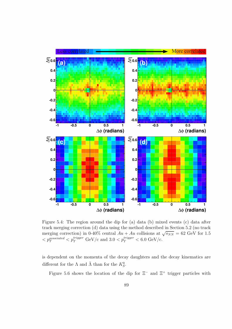
4000

4500

5000

5500

6000

(radians)φ∆

-1 -0.5 0 0.5 1

η∆

-0.6

-0.4

-0.2

0

0.2

0.4

0.6 (a)

0.7

0.75

0.8

0.85

0.9

0.95

1

1.05

(radians)φ∆

-1 -0.5 0 0.5 1

η∆

-0.6

-0.4

-0.2

0

0.2

0.4

0.6 (b)

24.2

24.4

24.6

24.8

25

25.2

25.4

25.6

25.8

26

26.2

(radians)φ∆

-1 -0.5 0 0.5 1

η∆

-0.6

-0.4

-0.2

0

0.2

0.4

0.6 (c)

5.05

5.1

5.15

5.2

5.25

5.3

5.35

5.4

(radians)φ∆

-1 -0.5 0 0.5 1

η∆

-0.6

-0.4

-0.2

0

0.2

0.4

0.6 (d)

Figure 5.4: The region around the dip for (a) data (b) mixed events (c) data aftertrack merging correction (d) data using the method described in Section 5.2 (no trackmerging correction) in 0-40% central Au + Au collisions at

√sNN = 62 GeV for 1.5

< passociatedT < ptrigger

T GeV/c and 3.0 < ptriggerT < 6.0 GeV/c.

is dependent on the momenta of the decay daughters and the decay kinematics are

different for the Λ and Λ than for the K0S.

Figure 5.6 shows the location of the dip for Ξ− and Ξ+ trigger particles with

89

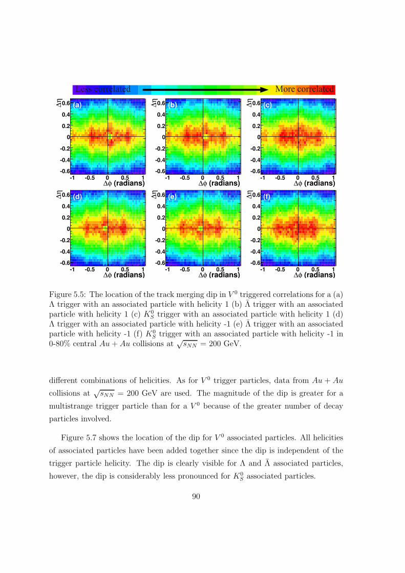
0.7

0.75

0.8

0.85

0.9

0.95

1

1.05

(radians)φ∆-1 -0.5 0 0.5 1

η∆

-0.6

-0.4

-0.2

0

0.2

0.4

0.6 (a)

0.65

0.7

0.75

0.8

0.85

0.9

0.95

1

1.05

(radians)φ∆-1 -0.5 0 0.5 1

η∆

-0.6

-0.4

-0.2

0

0.2

0.4

0.6 (b)

0.65

0.7

0.75

0.8

0.85

0.9

0.95

1

1.05

(radians)φ∆-1 -0.5 0 0.5 1

η∆

-0.6

-0.4

-0.2

0

0.2

0.4

0.6 (c)

0.65

0.7

0.75

0.8

0.85

0.9

0.95

1

1.05

(radians)φ∆-1 -0.5 0 0.5 1

η∆

-0.6

-0.4

-0.2

0

0.2

0.4

0.6 (d)

0.65

0.7

0.75

0.8

0.85

0.9

0.95

1

1.05

(radians)φ∆-1 -0.5 0 0.5 1

η∆

-0.6

-0.4

-0.2

0

0.2

0.4

0.6 (e)

0.7

0.75

0.8

0.85

0.9

0.95

1

1.05

(radians)φ∆-1 -0.5 0 0.5 1

η∆

-0.6

-0.4

-0.2

0

0.2

0.4

0.6 (f)

Figure 5.5: The location of the track merging dip in V 0 triggered correlations for a (a)Λ trigger with an associated particle with helicity 1 (b) Λ trigger with an associatedparticle with helicity 1 (c) K0

S trigger with an associated particle with helicity 1 (d)Λ trigger with an associated particle with helicity -1 (e) Λ trigger with an associatedparticle with helicity -1 (f) K0

S trigger with an associated particle with helicity -1 in0-80% central Au+ Au collisions at

√sNN = 200 GeV.

different combinations of helicities. As for V 0 trigger particles, data from Au + Au

collisions at√sNN = 200 GeV are used. The magnitude of the dip is greater for a

multistrange trigger particle than for a V 0 because of the greater number of decay

particles involved.

Figure 5.7 shows the location of the dip for V 0 associated particles. All helicities

of associated particles have been added together since the dip is independent of the

trigger particle helicity. The dip is clearly visible for Λ and Λ associated particles,

however, the dip is considerably less pronounced for K0S associated particles.

90

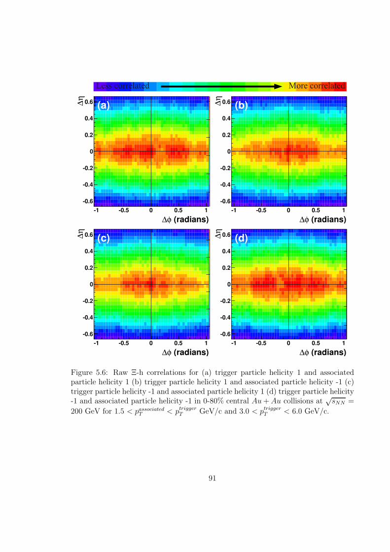
0.055

0.06

0.065

0.07

0.075

0.08

(radians)φ∆

-1 -0.5 0 0.5 1

η∆

-0.6

-0.4

-0.2

0

0.2

0.4

0.6 (a)

0.055

0.06

0.065

0.07

0.075

0.08

(radians)φ∆

-1 -0.5 0 0.5 1

η∆

-0.6

-0.4

-0.2

0

0.2

0.4

0.6 (b)

0.055

0.06

0.065

0.07

0.075

0.08

(radians)φ∆

-1 -0.5 0 0.5 1

η∆

-0.6

-0.4

-0.2

0

0.2

0.4

0.6 (c)

0.055

0.06

0.065

0.07

0.075

0.08

(radians)φ∆

-1 -0.5 0 0.5 1

η∆

-0.6

-0.4

-0.2

0

0.2

0.4

0.6 (d)

Figure 5.6: Raw Ξ-h correlations for (a) trigger particle helicity 1 and associatedparticle helicity 1 (b) trigger particle helicity 1 and associated particle helicity -1 (c)trigger particle helicity -1 and associated particle helicity 1 (d) trigger particle helicity-1 and associated particle helicity -1 in 0-80% central Au+Au collisions at

√sNN =

200 GeV for 1.5 < passociatedT < ptrigger

T GeV/c and 3.0 < ptriggerT < 6.0 GeV/c.

91

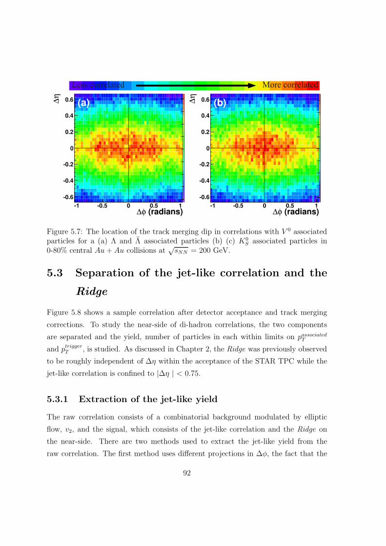
2.6

2.8

3

3.2

3.4

3.6

3.8

4

4.2

(radians)φ∆-1 -0.5 0 0.5 1

η∆

-0.6

-0.4

-0.2

0

0.2

0.4

0.6 (a)

1.3

1.4

1.5

1.6

1.7

1.8

1.9

2

2.1

(radians)φ∆-1 -0.5 0 0.5 1

η∆

-0.6

-0.4

-0.2

0

0.2

0.4

0.6 (b)

Figure 5.7: The location of the track merging dip in correlations with V 0 associatedparticles for a (a) Λ and Λ associated particles (b) (c) K0

S associated particles in0-80% central Au+ Au collisions at

√sNN = 200 GeV.

5.3 Separation of the jet-like correlation and the

Ridge

Figure 5.8 shows a sample correlation after detector acceptance and track merging

corrections. To study the near-side of di-hadron correlations, the two components

are separated and the yield, number of particles in each within limits on passociatedT

and ptriggerT , is studied. As discussed in Chapter 2, the Ridge was previously observed

to be roughly independent of ∆η within the acceptance of the STAR TPC while the

jet-like correlation is confined to |∆η | < 0.75.

5.3.1 Extraction of the jet-like yield

The raw correlation consists of a combinatorial background modulated by elliptic

flow, v2, and the signal, which consists of the jet-like correlation and the Ridge on

the near-side. There are two methods used to extract the jet-like yield from the

raw correlation. The first method uses different projections in ∆φ, the fact that the

92

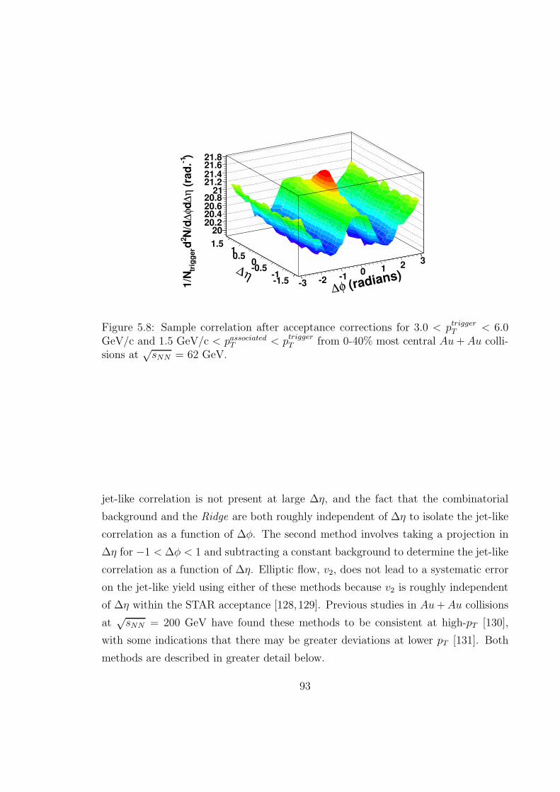
(radians)φ∆

-3 -2 -10 1 2 3

η∆-1.5-1

-0.50

0.51

1.5

)-1

(ra

d.

η∆

dφ

∆N

/d2

dtr

igg

er

1/N

2020.220.420.620.8

2121.221.421.621.8

Figure 5.8: Sample correlation after acceptance corrections for 3.0 < ptriggerT < 6.0

GeV/c and 1.5 GeV/c < passociatedT < ptrigger

T from 0-40% most central Au+Au colli-sions at

√sNN = 62 GeV.

jet-like correlation is not present at large ∆η, and the fact that the combinatorial

background and the Ridge are both roughly independent of ∆η to isolate the jet-like

correlation as a function of ∆φ. The second method involves taking a projection in

∆η for −1 < ∆φ < 1 and subtracting a constant background to determine the jet-like

correlation as a function of ∆η. Elliptic flow, v2, does not lead to a systematic error

on the jet-like yield using either of these methods because v2 is roughly independent

of ∆η within the STAR acceptance [128,129]. Previous studies in Au+Au collisions

at√sNN = 200 GeV have found these methods to be consistent at high-pT [130],

with some indications that there may be greater deviations at lower pT [131]. Both

methods are described in greater detail below.

93

∆φ method

To determine the jet-like yield, YJet, the projection of the distribution of particlesd2N

d∆φd∆ηis taken in two different ranges in pseudorapidity:

dYridge

d∆φ=

1

Ntrigger

−0.75∫

−1.75

d2N

d∆φd∆ηd∆η +

1

Ntrigger

1.75∫

0.75

d2N

d∆φd∆ηd∆η (5.2)

dYjet+ridge

d∆φ=

1

Ntrigger

0.75∫

−0.75

d2N

d∆φd∆ηd∆η (5.3)

where the former contains only the Ridge and the latter contains both the jet-like

correlation and the Ridge. The jet-like yield, YJet, is determined using bin counting

in the region −1 < ∆φ < 1:

Y ∆φjet =

1∫

−1

(dYjet+ridge

d∆φ− 0.75

1

dYridge

d∆φ)d∆φ. (5.4)

The factor in front of the second term is the ratio of the ∆η width in the region

containing the jet-like correlation and the Ridge to the width of the region containing

only the Ridge. In practice because the data have been reflected about ∆φ = 0 and

∆η = 0, the projections in ∆φ and ∆η and the bin counting are done over half of the

range and then scaled up to ensure that the errors are correct.

∆η method

In this method the projection of the distribution of particles d2Nd∆φd∆η

on the near-side

is taken:

1

Ntrigger

dN

d∆η=

1

Ntrigger

1∫

−1

d2N

d∆φd∆ηd∆φ. (5.5)

This contains both a background due to combinatorics and the Ridge, both of which

are independent of ∆η. The background is determined first by fitting a Gaussian

signal plus a constant background, A, to Equation 5.6 and then using the background

from that for background subtraction. If statistics permitted, the background could

94

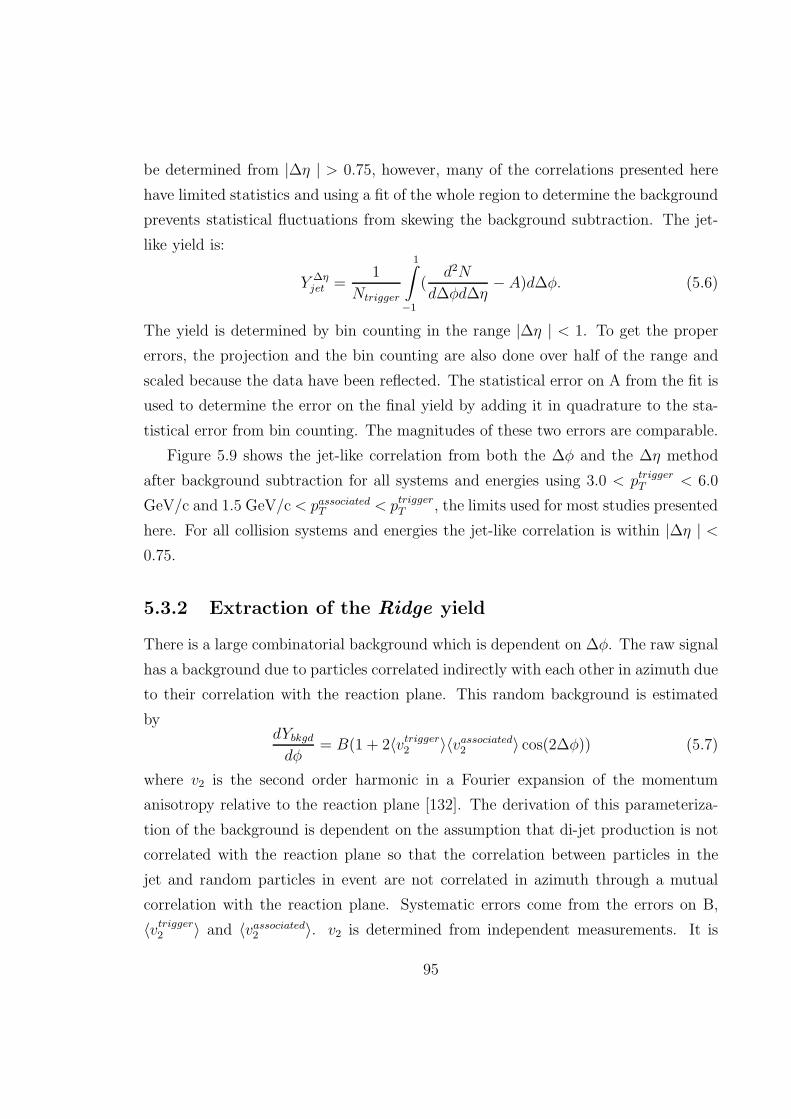
be determined from |∆η | > 0.75, however, many of the correlations presented here

have limited statistics and using a fit of the whole region to determine the background

prevents statistical fluctuations from skewing the background subtraction. The jet-

like yield is:

Y ∆ηjet =

1

Ntrigger

1∫

−1

(d2N

d∆φd∆η− A)d∆φ. (5.6)

The yield is determined by bin counting in the range |∆η | < 1. To get the proper

errors, the projection and the bin counting are also done over half of the range and

scaled because the data have been reflected. The statistical error on A from the fit is

used to determine the error on the final yield by adding it in quadrature to the sta-

tistical error from bin counting. The magnitudes of these two errors are comparable.

Figure 5.9 shows the jet-like correlation from both the ∆φ and the ∆η method

after background subtraction for all systems and energies using 3.0 < ptriggerT < 6.0

GeV/c and 1.5 GeV/c< passociatedT < ptrigger

T , the limits used for most studies presented

here. For all collision systems and energies the jet-like correlation is within |∆η | <0.75.

5.3.2 Extraction of the Ridge yield

There is a large combinatorial background which is dependent on ∆φ. The raw signal

has a background due to particles correlated indirectly with each other in azimuth due

to their correlation with the reaction plane. This random background is estimated

bydYbkgd

dφ= B(1 + 2〈vtrigger

2 〉〈vassociated2 〉 cos(2∆φ)) (5.7)

where v2 is the second order harmonic in a Fourier expansion of the momentum

anisotropy relative to the reaction plane [132]. The derivation of this parameteriza-

tion of the background is dependent on the assumption that di-jet production is not

correlated with the reaction plane so that the correlation between particles in the

jet and random particles in event are not correlated in azimuth through a mutual

correlation with the reaction plane. Systematic errors come from the errors on B,

〈vtrigger2 〉 and 〈vassociated

2 〉. v2 is determined from independent measurements. It is

95

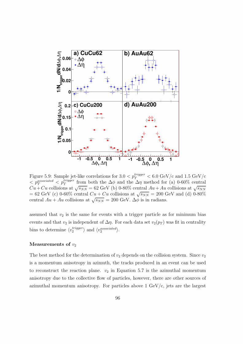
η

∆,φ

∆d

N/d

trig

ge

r1/N

0

0.02

0.04

0.06a) CuCu62

φ∆η∆

-0.01

0

0.01

0.02

0.03

0.04

0.05

0.06

0.07 b) AuAu62

η∆, φ∆-1 -0.5 0 0.5 1

η

∆,φ

∆d

N/d

trig

ge

r1

/N

0

0.05

0.1

0.15

0.2 c) CuCu200

φ∆η∆

η∆, φ∆-1 -0.5 0 0.5 1

0

0.05

0.1

0.15

0.2 d) AuAu200

Figure 5.9: Sample jet-like correlations for 3.0 < ptriggerT < 6.0 GeV/c and 1.5 GeV/c

< passociatedT < ptrigger

T from both the ∆φ and the ∆η method for (a) 0-60% centralCu+Cu collisions at

√sNN = 62 GeV (b) 0-80% central Au+Au collisions at

√sNN

= 62 GeV (c) 0-60% central Cu+ Cu collisions at√sNN = 200 GeV and (d) 0-80%

central Au+ Au collisions at√sNN = 200 GeV. ∆φ is in radians.

assumed that v2 is the same for events with a trigger particle as for minimum bias

events and that v2 is independent of ∆η. For each data set v2(pT ) was fit in centrality

bins to determine 〈vtrigger2 〉 and 〈vassociated

2 〉.

Measurements of v2

The best method for the determination of v2 depends on the collision system. Since v2

is a momentum anisotropy in azimuth, the tracks produced in an event can be used

to reconstruct the reaction plane. v2 in Equation 5.7 is the azimuthal momentum

anisotropy due to the collective flow of particles, however, there are other sources of

azimuthal momentum anisotropy. For particles above 1 GeV/c, jets are the largest

96

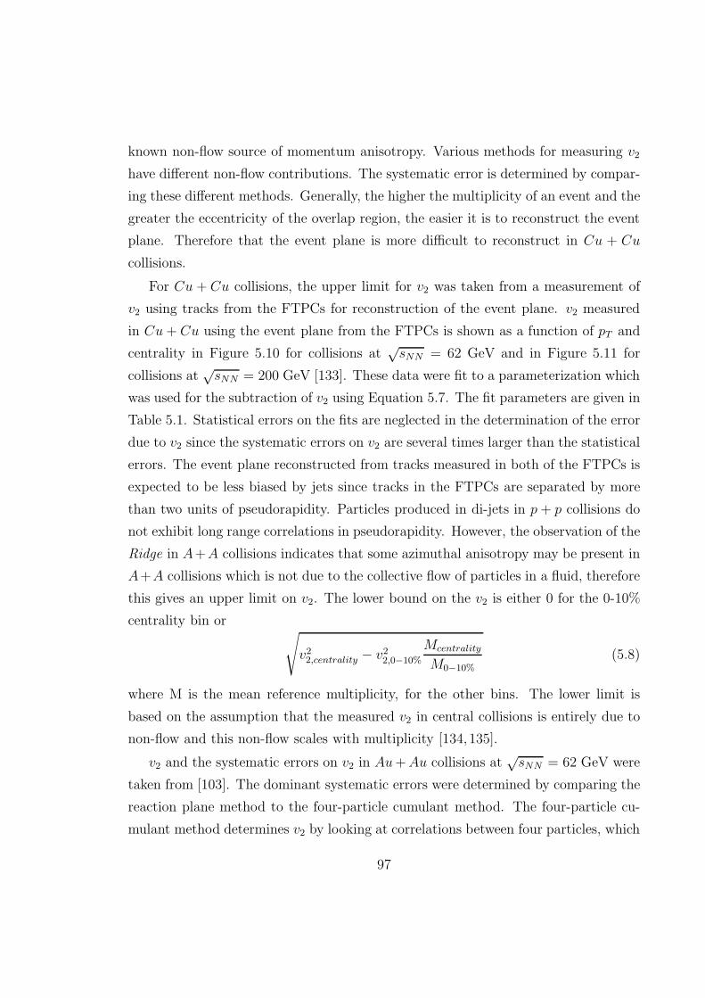
known non-flow source of momentum anisotropy. Various methods for measuring v2

have different non-flow contributions. The systematic error is determined by compar-

ing these different methods. Generally, the higher the multiplicity of an event and the

greater the eccentricity of the overlap region, the easier it is to reconstruct the event

plane. Therefore that the event plane is more difficult to reconstruct in Cu + Cu

collisions.

For Cu + Cu collisions, the upper limit for v2 was taken from a measurement of

v2 using tracks from the FTPCs for reconstruction of the event plane. v2 measured

in Cu+ Cu using the event plane from the FTPCs is shown as a function of pT and

centrality in Figure 5.10 for collisions at√sNN = 62 GeV and in Figure 5.11 for

collisions at√sNN = 200 GeV [133]. These data were fit to a parameterization which

was used for the subtraction of v2 using Equation 5.7. The fit parameters are given in

Table 5.1. Statistical errors on the fits are neglected in the determination of the error

due to v2 since the systematic errors on v2 are several times larger than the statistical

errors. The event plane reconstructed from tracks measured in both of the FTPCs is

expected to be less biased by jets since tracks in the FTPCs are separated by more

than two units of pseudorapidity. Particles produced in di-jets in p + p collisions do

not exhibit long range correlations in pseudorapidity. However, the observation of the

Ridge in A+A collisions indicates that some azimuthal anisotropy may be present in

A+A collisions which is not due to the collective flow of particles in a fluid, therefore

this gives an upper limit on v2. The lower bound on the v2 is either 0 for the 0-10%

centrality bin or√

v22,centrality − v2

2,0−10%

Mcentrality

M0−10%

(5.8)

where M is the mean reference multiplicity, for the other bins. The lower limit is

based on the assumption that the measured v2 in central collisions is entirely due to

non-flow and this non-flow scales with multiplicity [134, 135].

v2 and the systematic errors on v2 in Au+Au collisions at√sNN = 62 GeV were

taken from [103]. The dominant systematic errors were determined by comparing the

reaction plane method to the four-particle cumulant method. The four-particle cu-

mulant method determines v2 by looking at correlations between four particles, which

97

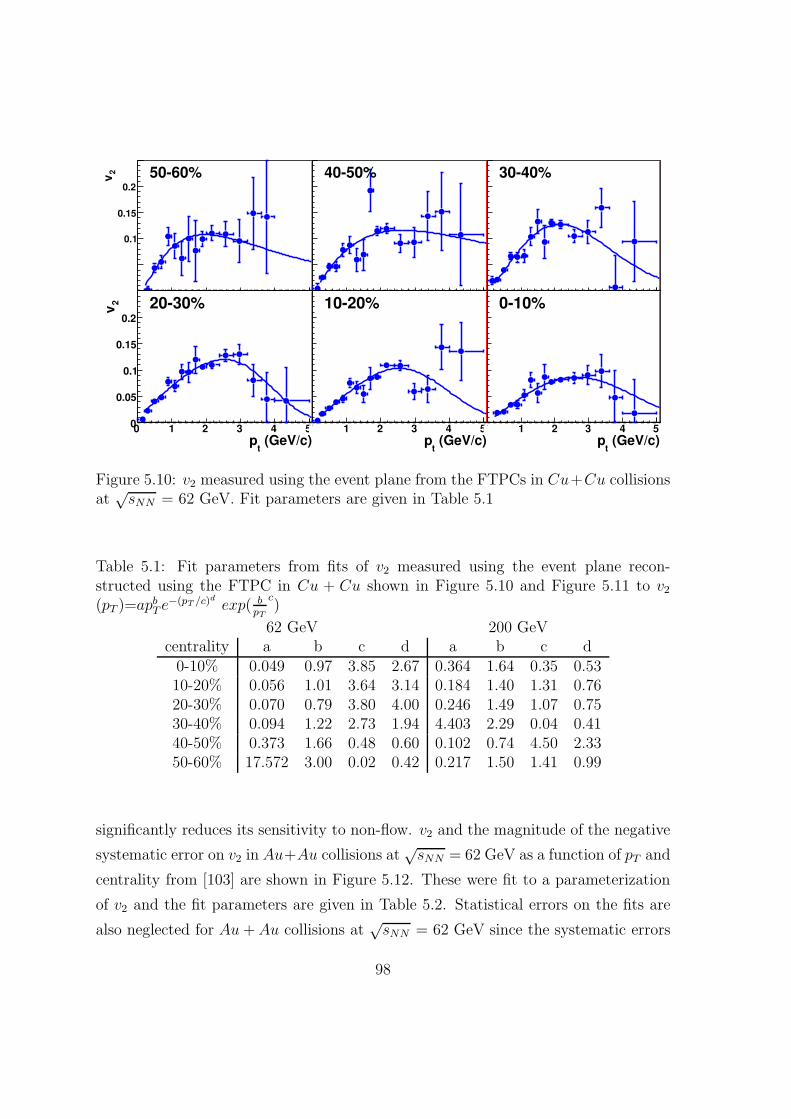
0 1 2 3 4 5

2v

0

0.05

0.1

0.15

0.2

0.25

50-60%

0 1 2 3 4 50

0.05

0.1

0.15

0.2

0.25

40-50%

0 1 2 3 4 50

0.05

0.1

0.15

0.2

0.25

30-40%

(GeV/c)t

p0 1 2 3 4 5

2v

0

0.05

0.1

0.15

0.2

0.25

20-30%

(GeV/c)t

p0 1 2 3 4 50

0.05

0.1

0.15

0.2

0.25

10-20%

(GeV/c)t

p0 1 2 3 4 50

0.05

0.1

0.15

0.2

0.25

0-10%

Figure 5.10: v2 measured using the event plane from the FTPCs in Cu+Cu collisionsat

√sNN = 62 GeV. Fit parameters are given in Table 5.1

Table 5.1: Fit parameters from fits of v2 measured using the event plane recon-structed using the FTPC in Cu + Cu shown in Figure 5.10 and Figure 5.11 to v2

(pT )=apbT e

−(pT /c)d

exp( bpT

c)

62 GeV 200 GeVcentrality a b c d a b c d

0-10% 0.049 0.97 3.85 2.67 0.364 1.64 0.35 0.5310-20% 0.056 1.01 3.64 3.14 0.184 1.40 1.31 0.7620-30% 0.070 0.79 3.80 4.00 0.246 1.49 1.07 0.7530-40% 0.094 1.22 2.73 1.94 4.403 2.29 0.04 0.4140-50% 0.373 1.66 0.48 0.60 0.102 0.74 4.50 2.3350-60% 17.572 3.00 0.02 0.42 0.217 1.50 1.41 0.99

significantly reduces its sensitivity to non-flow. v2 and the magnitude of the negative

systematic error on v2 in Au+Au collisions at√sNN = 62 GeV as a function of pT and

centrality from [103] are shown in Figure 5.12. These were fit to a parameterization

of v2 and the fit parameters are given in Table 5.2. Statistical errors on the fits are

also neglected for Au+Au collisions at√sNN = 62 GeV since the systematic errors

98

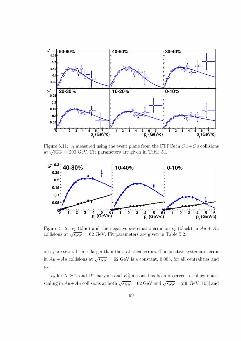
0 1 2 3 4 5 6 7 8

2v

0

0.05

0.1

0.15

0.2

0.25

0.350-60%

0 1 2 3 4 5 6 7 80

0.05

0.1

0.15

0.2

0.25

0.3

40-50%

0 1 2 3 4 5 6 7 80

0.05

0.1

0.15

0.2

0.25

0.3

30-40%

(GeV/c)t

p0 1 2 3 4 5 6 7 8

2v

0

0.05

0.1

0.15

0.2

0.25

0.320-30%

(GeV/c)t

p0 1 2 3 4 5 6 7 80

0.05

0.1

0.15

0.2

0.25

0.310-20%

(GeV/c)t

p0 1 2 3 4 5 6 7 80

0.05

0.1

0.15

0.2

0.25

0.30-10%

Figure 5.11: v2 measured using the event plane from the FTPCs in Cu+Cu collisionsat

√sNN = 200 GeV. Fit parameters are given in Table 5.1

(GeV/c)t

p0 1 2 3 4 5 6

2v

0

0.05

0.1

0.15

0.2

0.25

0.340-80%

(GeV/c)t

p0 1 2 3 4 5 6

0

0.05

0.1

0.15

0.2

0.25

0.3

10-40%

(GeV/c)t

p0 1 2 3 4 5 6

0

0.05

0.1

0.15

0.2

0.25

0.3

0-10%

Figure 5.12: v2 (blue) and the negative systematic error on v2 (black) in Au + Aucollisions at

√sNN = 62 GeV. Fit parameters are given in Table 5.2.

on v2 are several times larger than the statistical errors. The positive systematic error

in Au+Au collisions at√sNN = 62 GeV is a constant, 0.003, for all centralities and

pT .

v2 for Λ, Ξ−, and Ω− baryons and K0S mesons has been observed to follow quark

scaling in Au+Au collisions at both√sNN = 62 GeV and

√sNN = 200 GeV [103] and

99

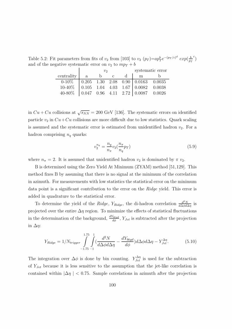
Table 5.2: Fit parameters from fits of v2 from [103] to v2 (pT )=apbT e

−(pT /c)d

exp( bpT

c)

and of the negative systematic error on v2 to mpT + b

v2 systematic errorcentrality a b c d m b

0-10% 0.205 1.30 2.08 0.90 0.0163 0.003510-40% 0.105 1.04 4.03 1.67 0.0082 0.003840-80% 0.047 0.96 4.11 2.72 0.0087 0.0026

in Cu+Cu collisions at√sNN = 200 GeV [136]. The systematic errors on identified

particle v2 in Cu+Cu collisions are more difficult due to low statistics. Quark scaling

is assumed and the systematic error is estimated from unidentified hadron v2. For a

hadron comprising nq quarks:

vnq

2 =nq

nπv2(

nπ

nqpT ) (5.9)

where nπ = 2. It is assumed that unidentified hadron v2 is dominated by π v2.

B is determined using the Zero Yield At Minimum (ZYAM) method [51,129]. This

method fixes B by assuming that there is no signal at the minimum of the correlation

in azimuth. For measurements with low statistics the statistical error on the minimum

data point is a significant contribution to the error on the Ridge yield. This error is

added in quadrature to the statistical error.

To determine the yield of the Ridge, YRidge, the di-hadron correlation d2Nd∆φd∆η

is

projected over the entire ∆η region. To minimize the effects of statistical fluctuations

in the determination of the background,dYbkgd

dφ, YJet is subtracted after the projection

in ∆η:

YRidge = 1/Ntrigger

1.75∫

−1.75

1∫

−1

(d2N

d∆φd∆η− dYbkgd

dφ)d∆φd∆η − Y ∆η

Jet . (5.10)

The integration over ∆φ is done by bin counting. Y ∆ηJet is used for the subtraction

of YJet because it is less sensitive to the assumption that the jet-like correlation is

contained within |∆η | < 0.75. Sample correlations in azimuth after the projection

100

-3 -2 -1 0 1 2 3

)-1

(ra

d.

φ∆

dN

/dtr

ig1

/N

0.95

1

1.05

1.1

1.15 a) CuCu62

-3 -2 -1 0 1 2 3

3.8

3.9

4

4.1

4.2

4.3b) AuAu62

(radians)φ∆-3 -2 -1 0 1 2 3

)-1

(ra

d.

φ∆

dN

/dtr

ig1

/N

1.8

1.9

2

2.1

2.2

2.3

2.4 c) CuCu200

(radians)φ∆-3 -2 -1 0 1 2 3

6.6

6.8

7

7.2

7.4

7.6

7.8d) AuAu200

Figure 5.13: Sample correlations in ∆φ integrated over |∆η | < 1.75 for 3.0 < ptriggerT

< 6.0 GeV/c and 1.5 GeV/c < passociatedT < ptrigger

T from (a) 0-60% central Cu + Cucollisions at

√sNN = 62 GeV (b) 0-80% central Au + Au collisions at

√sNN = 62

GeV (c) 0-60% central Cu+Cu collisions at√sNN = 200 GeV and (d) 0-80% central

Au+Au collisions at√sNN = 200 GeV showing the background level and shape for

high and low bounds on v2 from each data set.

over ∆η are shown in Figure 5.13 for all data sets. These correlations show the

background level and shape for the high and low bounds on v2.

101

102

Chapter 6

Results

6.1 The jet-like correlation

If the jet-like correlation is produced by fragmentation, no dependence on collision

system or system size would be expected. The particle ratios of the jet-like correlation

should be consistent with what was observed in p+ p collisions since p+ p collisions

are expected to be dominated by jet production at high-pT . The jet-like yield should

increase with ptriggerT because higher pT trigger particles come on average from higher

energy jets and the spectra of particles in the jet-like correlation should be harder than

that observed in the inclusive. Studies of the jet-like yield as a function of collision

system and energy were done for unidentified hadrons for Cu + Cu and Au + Au

collisions at√sNN = 62 GeV and

√sNN = 200 GeV to determine whether the data

are consistent with the jet-like correlation being produced by fragmentation.

6.1.1 Energy and system dependence

The dependence of jet-like yield, YJet, on ptriggerT is shown in Figure 6.1 for Cu+ Cu

and Au + Au collisions at√sNN = 62 GeV and d + Au, Cu + Cu, and Au + Au

collisions at√sNN = 200 GeV. No Ridge is observed in d + Au collisions so it was

not necessary to subtract the Ridge. The jet-like yields are the same as a function of

ptriggerT within errors for all systems at a given collision energy.

103

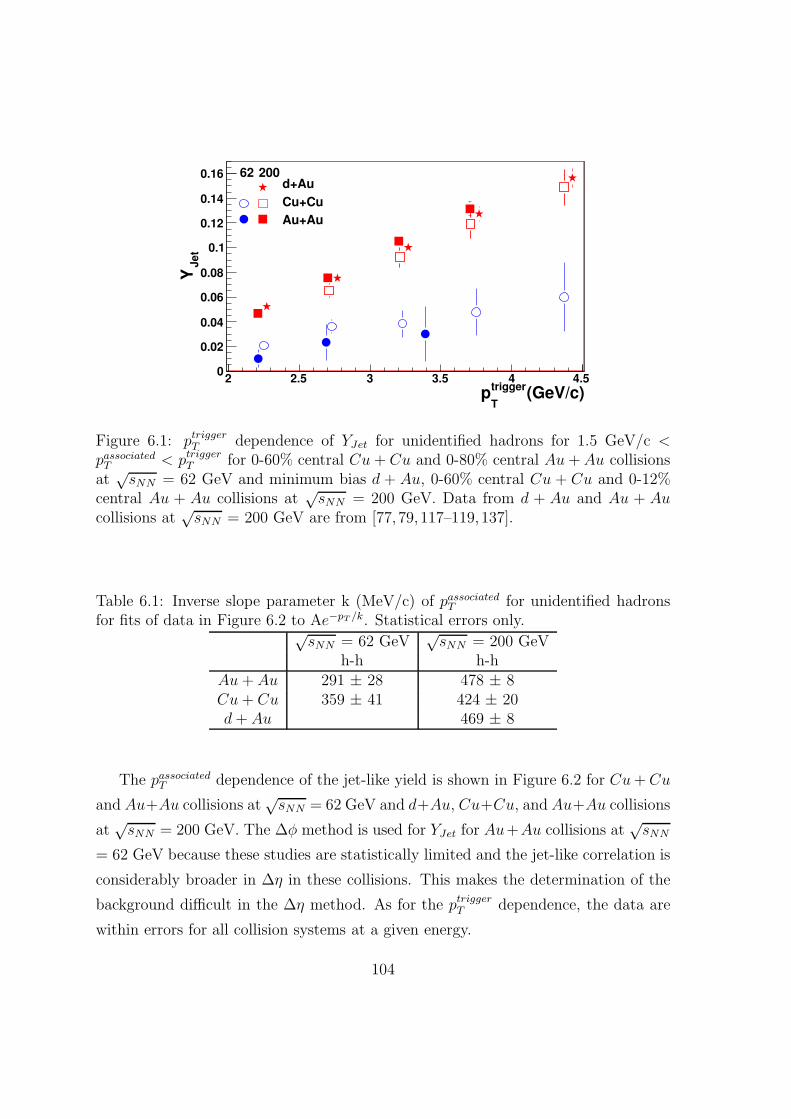
(GeV/c)trigger

Tp

2 2.5 3 3.5 4 4.5

Je

tY

0

0.02

0.04

0.06

0.08

0.1

0.12

0.14

0.16 62

200

d+Au

Cu+Cu

Au+Au

Figure 6.1: ptriggerT dependence of YJet for unidentified hadrons for 1.5 GeV/c <

passociatedT < ptrigger

T for 0-60% central Cu+ Cu and 0-80% central Au+Au collisionsat

√sNN = 62 GeV and minimum bias d + Au, 0-60% central Cu + Cu and 0-12%

central Au + Au collisions at√sNN = 200 GeV. Data from d + Au and Au + Au

collisions at√sNN = 200 GeV are from [77,79, 117–119,137].

Table 6.1: Inverse slope parameter k (MeV/c) of passociatedT for unidentified hadrons

for fits of data in Figure 6.2 to Ae−pT /k. Statistical errors only.√sNN = 62 GeV

√sNN = 200 GeV

h-h h-hAu+ Au 291 ± 28 478 ± 8Cu+ Cu 359 ± 41 424 ± 20d+ Au 469 ± 8

The passociatedT dependence of the jet-like yield is shown in Figure 6.2 for Cu+Cu

and Au+Au collisions at√sNN = 62 GeV and d+Au, Cu+Cu, and Au+Au collisions

at√sNN = 200 GeV. The ∆φ method is used for YJet for Au+Au collisions at

√sNN

= 62 GeV because these studies are statistically limited and the jet-like correlation is

considerably broader in ∆η in these collisions. This makes the determination of the

background difficult in the ∆η method. As for the ptriggerT dependence, the data are

within errors for all collision systems at a given energy.

104

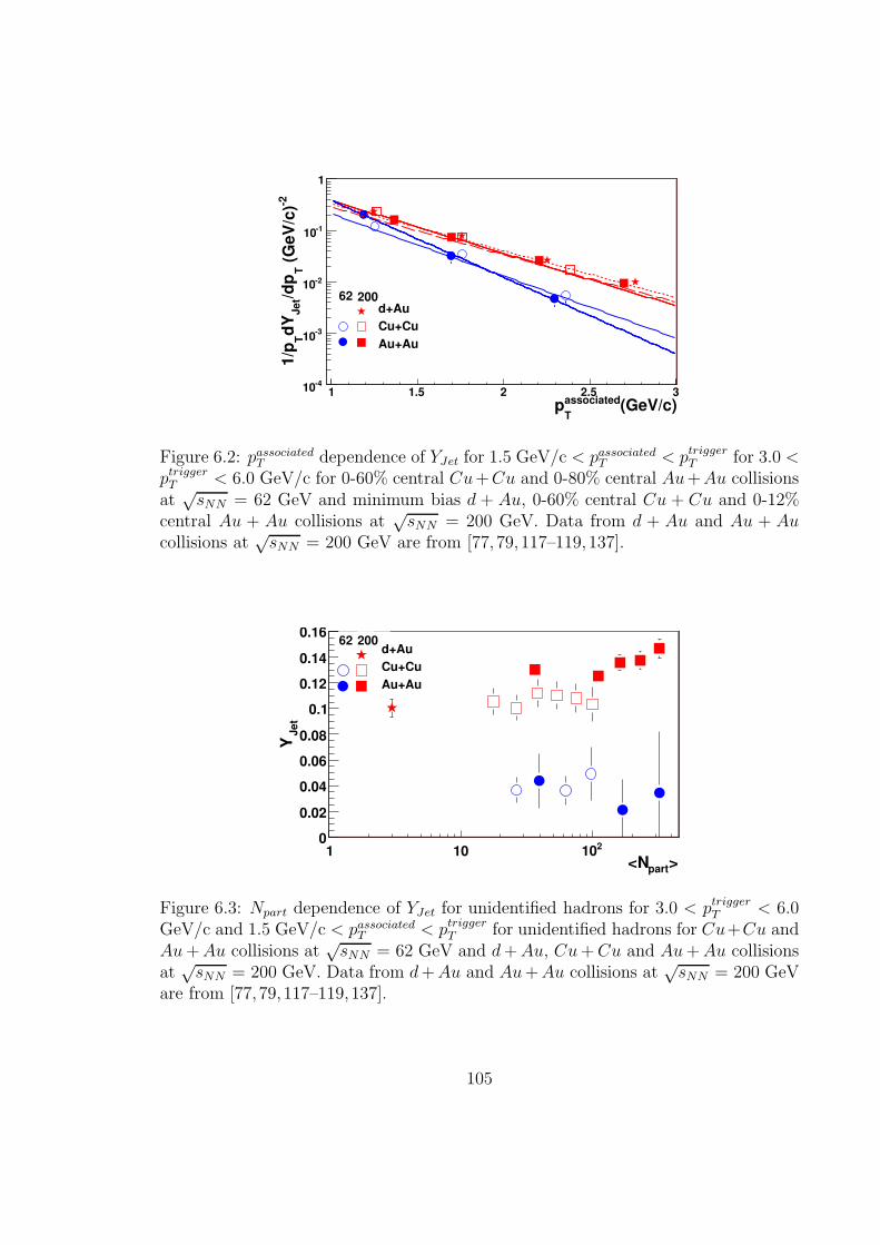
(GeV/c)associated

Tp

1 1.5 2 2.5 3

-2 (

GeV

/c)

T/d

pJet

dY

T1/p

-410

-310

-210

-110

1

62

200

d+Au

Cu+Cu

Au+Au

Figure 6.2: passociatedT dependence of YJet for 1.5 GeV/c < passociated

T < ptriggerT for 3.0 <

ptriggerT < 6.0 GeV/c for 0-60% central Cu+Cu and 0-80% central Au+Au collisions

at√sNN = 62 GeV and minimum bias d + Au, 0-60% central Cu + Cu and 0-12%

central Au + Au collisions at√sNN = 200 GeV. Data from d + Au and Au + Au

collisions at√sNN = 200 GeV are from [77,79, 117–119,137].

>part<N1 10 210

Jet

Y

0

0.02

0.04

0.06

0.08

0.1

0.12

0.14

0.1662

200

d+Au

Cu+Cu

Au+Au

Figure 6.3: Npart dependence of YJet for unidentified hadrons for 3.0 < ptriggerT < 6.0

GeV/c and 1.5 GeV/c < passociatedT < ptrigger

T for unidentified hadrons for Cu+Cu andAu+Au collisions at

√sNN = 62 GeV and d+Au, Cu+Cu and Au+Au collisions

at√sNN = 200 GeV. Data from d+Au and Au+Au collisions at

√sNN = 200 GeV

are from [77,79, 117–119,137].

105

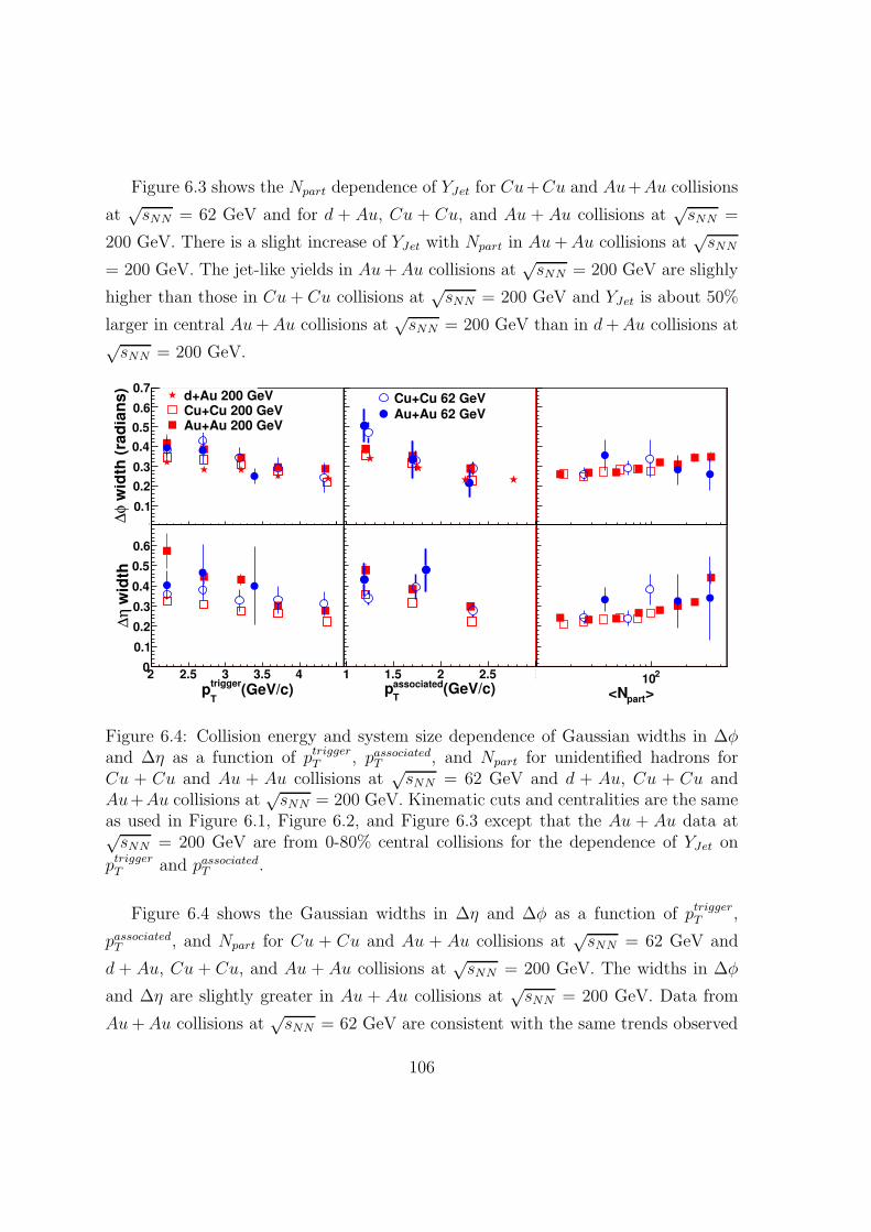
Figure 6.3 shows the Npart dependence of YJet for Cu+Cu and Au+Au collisions

at√sNN = 62 GeV and for d + Au, Cu + Cu, and Au + Au collisions at

√sNN =

200 GeV. There is a slight increase of YJet with Npart in Au+Au collisions at√sNN

= 200 GeV. The jet-like yields in Au+Au collisions at√sNN = 200 GeV are slighly

higher than those in Cu+ Cu collisions at√sNN = 200 GeV and YJet is about 50%

larger in central Au+Au collisions at√sNN = 200 GeV than in d+Au collisions at

√sNN = 200 GeV.

2 2.5 3 3.5 4 4.5

wid

th (

rad

ian

s)

φ∆

0

0.1

0.2

0.3

0.4

0.5

0.6

0.7d+Au 200 GeVCu+Cu 200 GeVAu+Au 200 GeV

1 1.5 2 2.5 3

Cu+Cu 62 GeVAu+Au 62 GeV

0

0.1

0.2

0.3

0.4

0.5

0.6

0.7

(GeV/c)trigger

Tp

2 2.5 3 3.5 4 4.5

wid

thη

∆

0

0.1

0.2

0.3

0.4

0.5

0.6

0.7

(GeV/c)associated

Tp

1 1.5 2 2.5 3

>part<N

210

0

0.1

0.2

0.3

0.4

0.5

0.6

0.7

Figure 6.4: Collision energy and system size dependence of Gaussian widths in ∆φand ∆η as a function of ptrigger

T , passociatedT , and Npart for unidentified hadrons for

Cu + Cu and Au + Au collisions at√sNN = 62 GeV and d + Au, Cu + Cu and

Au+Au collisions at√sNN = 200 GeV. Kinematic cuts and centralities are the same

as used in Figure 6.1, Figure 6.2, and Figure 6.3 except that the Au + Au data at√sNN = 200 GeV are from 0-80% central collisions for the dependence of YJet on

ptriggerT and passociated

T .

Figure 6.4 shows the Gaussian widths in ∆η and ∆φ as a function of ptriggerT ,

passociatedT , and Npart for Cu + Cu and Au + Au collisions at

√sNN = 62 GeV and

d + Au, Cu + Cu, and Au + Au collisions at√sNN = 200 GeV. The widths in ∆φ

and ∆η are slightly greater in Au + Au collisions at√sNN = 200 GeV. Data from

Au+Au collisions at√sNN = 62 GeV are consistent with the same trends observed

106

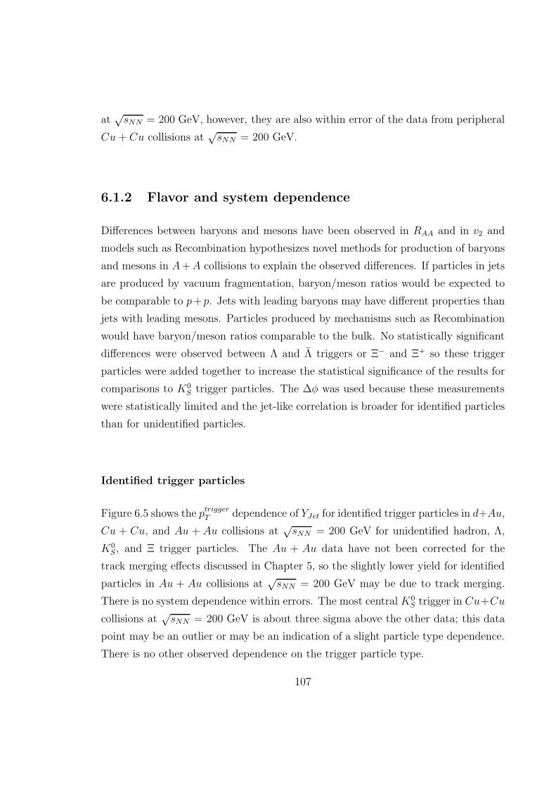
at√sNN = 200 GeV, however, they are also within error of the data from peripheral

Cu+ Cu collisions at√sNN = 200 GeV.

6.1.2 Flavor and system dependence

Differences between baryons and mesons have been observed in RAA and in v2 and

models such as Recombination hypothesizes novel methods for production of baryons

and mesons in A+A collisions to explain the observed differences. If particles in jets

are produced by vacuum fragmentation, baryon/meson ratios would be expected to

be comparable to p+p. Jets with leading baryons may have different properties than

jets with leading mesons. Particles produced by mechanisms such as Recombination

would have baryon/meson ratios comparable to the bulk. No statistically significant

differences were observed between Λ and Λ triggers or Ξ− and Ξ+ so these trigger

particles were added together to increase the statistical significance of the results for

comparisons to K0S trigger particles. The ∆φ was used because these measurements

were statistically limited and the jet-like correlation is broader for identified particles

than for unidentified particles.

Identified trigger particles

Figure 6.5 shows the ptriggerT dependence of YJet for identified trigger particles in d+Au,

Cu + Cu, and Au + Au collisions at√sNN = 200 GeV for unidentified hadron, Λ,

K0S, and Ξ trigger particles. The Au + Au data have not been corrected for the

track merging effects discussed in Chapter 5, so the slightly lower yield for identified

particles in Au + Au collisions at√sNN = 200 GeV may be due to track merging.

There is no system dependence within errors. The most central K0S trigger in Cu+Cu

collisions at√sNN = 200 GeV is about three sigma above the other data; this data

point may be an outlier or may be an indication of a slight particle type dependence.

There is no other observed dependence on the trigger particle type.

107

(GeV/c)trigger

Tp

2 2.5 3 3.5 4 4.5 5

Je

tY

0

0.05

0.1

0.15

0.2

0.25

0.3Cu

Au

h-h

-hΛ

-hS

0K

-hΞ

Figure 6.5: ptriggerT dependence of YJet for 1.5 GeV/c < passociated

T < ptriggerT in 0-60%

central Cu + Cu and 0-12% central Au + Au collisions at√sNN = 200 GeV for

unidentified hadrons, Λ, K0S, and Ξ trigger particles. Data from Au + Au collisions

at√sNN = 200 GeV are from [77]. The identified trigger particle data have been

horizontally offset for visibility. The Au + Au data have not been corrected for thetrack merging effects discussed in Chapter 5.

The passociatedT dependence of YJet for unidentified hadrons, Λ, K0

S, and Ξ trigger

particles is shown in Figure 6.6. Due to limited statistics, it was only possible to

extract YJet for two bins in passociatedT for Λ and K0

S trigger particles and one bin bor Ξ

trigger particles. The jet-like yields from identified trigger particles are within errors

of the jet-like yields for unidentified hadron trigger particles. The data in Au + Au

collisions at√sNN = 200 GeV also showed no dependence on trigger particle type [77].

The Npart dependence of YJet is shown in Figure 6.7 for Λ, K0S, and Ξ trigger

particles. The Au + Au data have not been corrected for track merging effects, and

this may explain the difference between identified trigger particles and unidentified

trigger particles.

No statistically significant differences between different trigger particles are ob-

served for the jet-like correlations, including non-strange, singly strange, and doubly

strange hadrons. Studies in Au + Au collisions at√sNN = 200 GeV indicated that

there is no trigger particle dependence for even the trebly strange Ω [81, 138].

108

(GeV/c)associated

Tp

1 1.5 2 2.5 3

-2 (

GeV

/c)

T/d

pJet

dY

T1/p

-310

-210

-110

1

h-h

-hΛ

-hS0

K

-hΞ

Figure 6.6: passociatedT dependence of YJet for 3.0 < ptrigger

T < 6.0 GeV/c in 0-60%central Cu+Cu collisions at

√sNN = 200 GeV for unidentified hadrons, Λ, K0

S, andΞ trigger particles. The line is from a fit of the h-h data to Ae−pT /k. The inverseslope parameter is given in Table 6.1. The identified trigger particle data have beenhorizontally offset for visibility.

>part<N1 10 210

Jet

Y

0

0.05

0.1

0.15

0.2

0.25 Au

Cu

d+Au

h-h-h

S

0K-hΛ-hΞ

Figure 6.7: Npart dependence of YJet for 3.0 < ptriggerT < 6.0 GeV/c and 1.5 GeV/c <

passociatedT < ptrigger

T for identified trigger particles in d+ Au, Cu+ Cu, and Au+ Aucollisions at

√sNN = 200 GeV for Λ, K0

S, and Ξ trigger particles. Data from d+Auand Au+Au collisions at

√sNN = 200 GeV are from [77,79,117–119]. The Au+Au

data have not been corrected for the track merging effects discussed in Chapter 5.

109

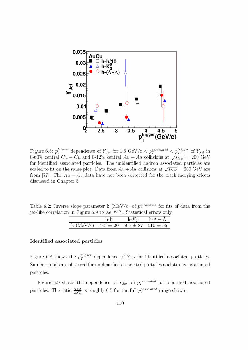
(GeV/c)trigger

Tp

2 2.5 3 3.5 4 4.5 5

Jet

Y

0

0.005

0.01

0.015

0.02

0.025

0.03

0.035Cu

Au

h-h/10

S0

h-K)Λ+Λh-(

Figure 6.8: ptriggerT dependence of YJet for 1.5 GeV/c < passociated

T < ptriggerT of YJet in

0-60% central Cu + Cu and 0-12% central Au + Au collisions at√sNN = 200 GeV

for identified associated particles. The unidentified hadron associated particles arescaled to fit on the same plot. Data from Au+Au collisions at

√sNN = 200 GeV are

from [77]. The Au + Au data have not been corrected for the track merging effectsdiscussed in Chapter 5.

Table 6.2: Inverse slope parameter k (MeV/c) of passociatedT for fits of data from the

jet-like correlation in Figure 6.9 to Ae−pT /k. Statistical errors only.

h-h h-K0S h-Λ + Λ

k (MeV/c) 445 ± 20 505 ± 87 510 ± 55

Identified associated particles

Figure 6.8 shows the ptriggerT dependence of YJet for identified associated particles.

Similar trends are observed for unidentified associated particles and strange associated

particles.

Figure 6.9 shows the dependence of YJet on passociatedT for identified associated

particles. The ratio Λ+Λ2K0

S

is roughly 0.5 for the full passociatedT range shown.

110

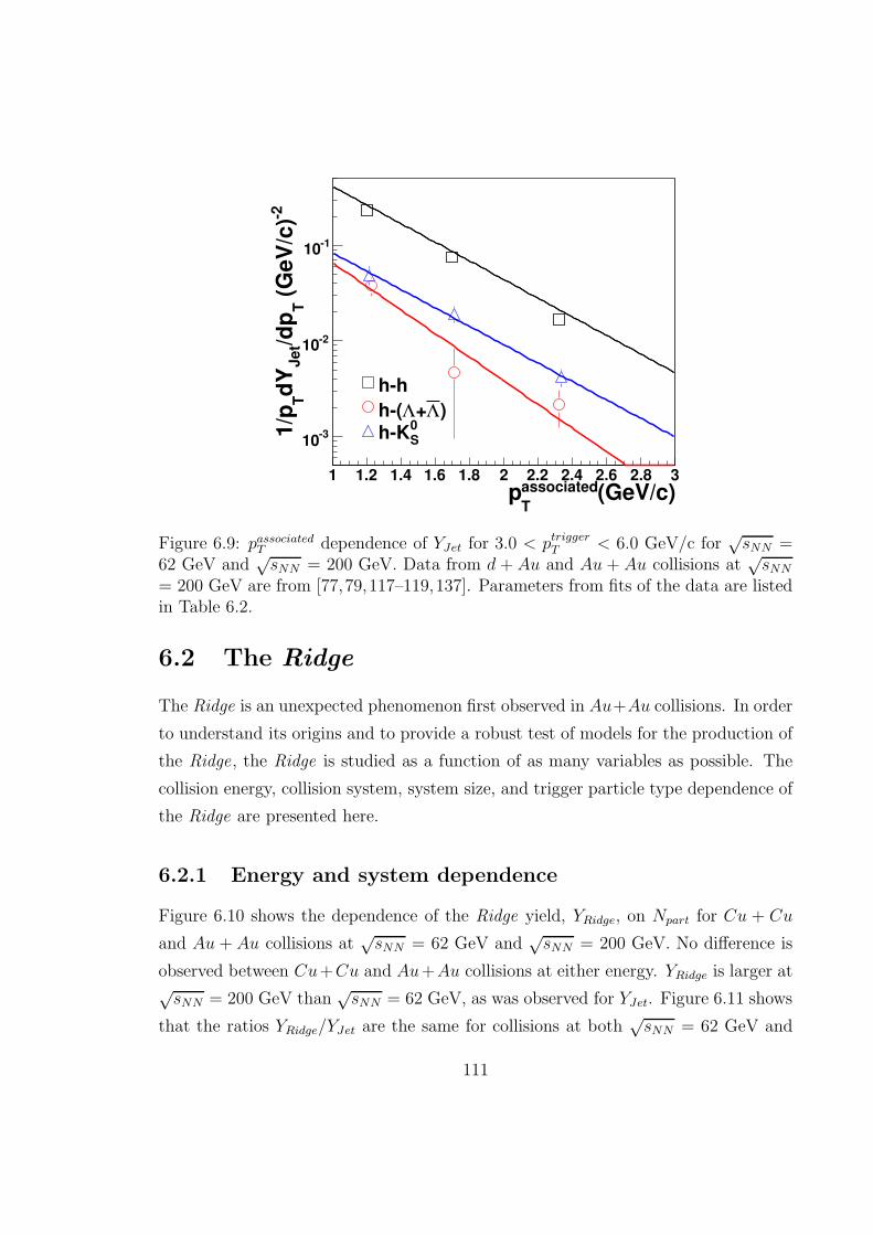
(GeV/c)associated

Tp

1 1.2 1.4 1.6 1.8 2 2.2 2.4 2.6 2.8 3

-2 (

Ge

V/c

)T

/dp

Je

td

YT

1/p

-310

-210

-110

h-h

)Λ+Λ h-(

S0

h-K

Figure 6.9: passociatedT dependence of YJet for 3.0 < ptrigger

T < 6.0 GeV/c for√sNN =

62 GeV and√sNN = 200 GeV. Data from d + Au and Au + Au collisions at

√sNN

= 200 GeV are from [77,79,117–119,137]. Parameters from fits of the data are listedin Table 6.2.

6.2 The Ridge

The Ridge is an unexpected phenomenon first observed in Au+Au collisions. In order

to understand its origins and to provide a robust test of models for the production of

the Ridge, the Ridge is studied as a function of as many variables as possible. The

collision energy, collision system, system size, and trigger particle type dependence of

the Ridge are presented here.

6.2.1 Energy and system dependence

Figure 6.10 shows the dependence of the Ridge yield, YRidge, on Npart for Cu + Cu

and Au + Au collisions at√sNN = 62 GeV and

√sNN = 200 GeV. No difference is

observed between Cu+Cu and Au+Au collisions at either energy. YRidge is larger at√sNN = 200 GeV than

√sNN = 62 GeV, as was observed for YJet. Figure 6.11 shows

that the ratios YRidge/YJet are the same for collisions at both√sNN = 62 GeV and

111

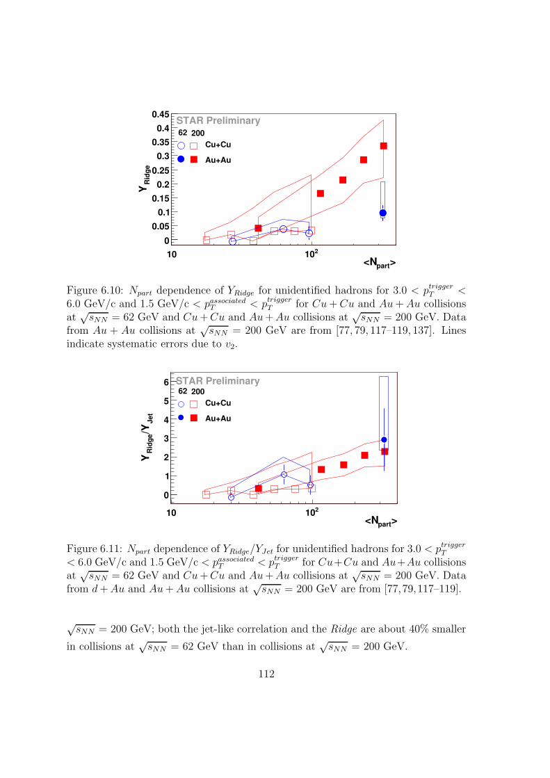
>part<N10 210

Rid

ge

Y

0

0.05

0.1

0.15

0.2

0.25

0.3

0.35

0.4

0.45STAR Preliminary62

200

Cu+Cu

Au+Au

Figure 6.10: Npart dependence of YRidge for unidentified hadrons for 3.0 < ptriggerT <

6.0 GeV/c and 1.5 GeV/c < passociatedT < ptrigger

T for Cu+Cu and Au+Au collisionsat

√sNN = 62 GeV and Cu+Cu and Au+Au collisions at

√sNN = 200 GeV. Data

from Au + Au collisions at√sNN = 200 GeV are from [77, 79, 117–119, 137]. Lines

indicate systematic errors due to v2.

>part<N10 210

Jet

/YR

idg

eY

0

1

2

3

4

5

662

200

Cu+Cu

Au+Au

STAR Preliminary

Figure 6.11: Npart dependence of YRidge/YJet for unidentified hadrons for 3.0 < ptriggerT

< 6.0 GeV/c and 1.5 GeV/c < passociatedT < ptrigger

T for Cu+Cu and Au+Au collisionsat

√sNN = 62 GeV and Cu+Cu and Au+Au collisions at

√sNN = 200 GeV. Data

from d+Au and Au+Au collisions at√sNN = 200 GeV are from [77,79,117–119].

√sNN = 200 GeV; both the jet-like correlation and the Ridge are about 40% smaller

in collisions at√sNN = 62 GeV than in collisions at

√sNN = 200 GeV.

112

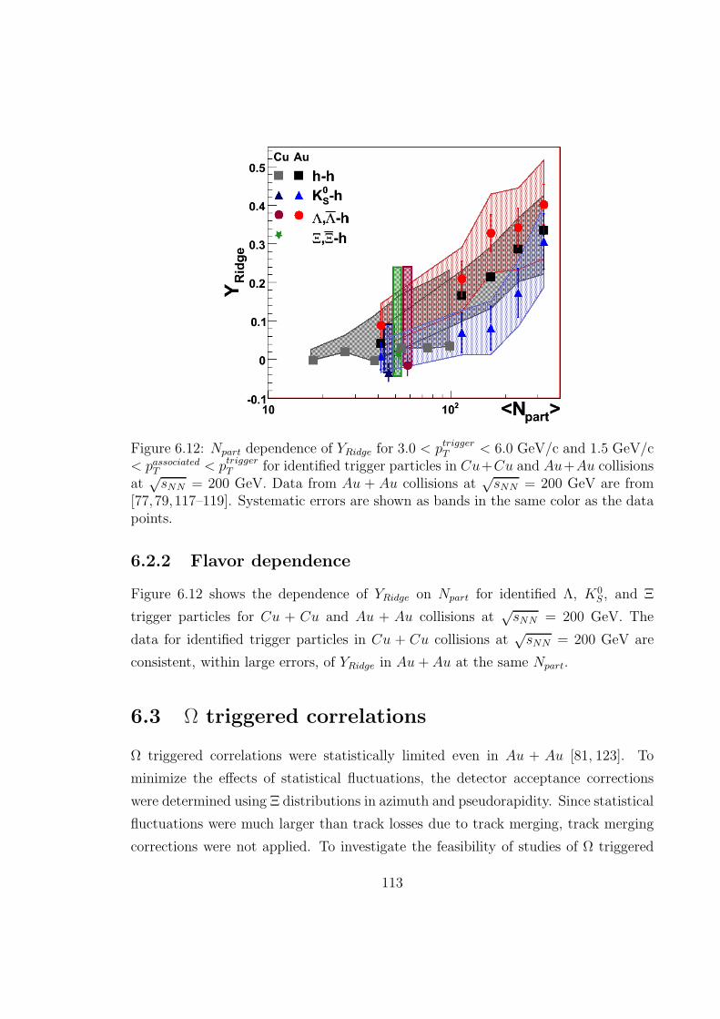
Figure 6.12: Npart dependence of YRidge for 3.0 < ptriggerT < 6.0 GeV/c and 1.5 GeV/c

< passociatedT < ptrigger

T for identified trigger particles in Cu+Cu and Au+Au collisionsat

√sNN = 200 GeV. Data from Au + Au collisions at

√sNN = 200 GeV are from

[77,79,117–119]. Systematic errors are shown as bands in the same color as the datapoints.

6.2.2 Flavor dependence

Figure 6.12 shows the dependence of YRidge on Npart for identified Λ, K0S, and Ξ

trigger particles for Cu + Cu and Au + Au collisions at√sNN = 200 GeV. The

data for identified trigger particles in Cu + Cu collisions at√sNN = 200 GeV are

consistent, within large errors, of YRidge in Au+ Au at the same Npart.

6.3 Ω triggered correlations

Ω triggered correlations were statistically limited even in Au + Au [81, 123]. To

minimize the effects of statistical fluctuations, the detector acceptance corrections

were determined using Ξ distributions in azimuth and pseudorapidity. Since statistical

fluctuations were much larger than track losses due to track merging, track merging

corrections were not applied. To investigate the feasibility of studies of Ω triggered

113

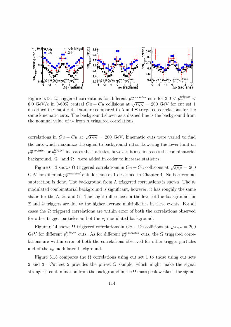
(radians)φ∆-3 -2 -1 0 1 2 3

-1

(ra

d.)

φ∆

dN

/dtr

igg

er

1/N

8.5

9

9.5

10

10.5 -hΛ-hΞ

-h bkgdΛ-hΩ

trigger

T<p

assoc

T(a) 1.0 GeV/c<p

(radians)φ∆-3 -2 -1 0 1 2 3

φ∆

dN

/dtr

igg

er

1/N

2.3

2.4

2.5

2.6

2.7

2.8

2.9

trigger

T<p

assoc

T(b) 1.5 GeV/c<p

(radians)φ∆-3 -2 -1 0 1 2 3

φ∆

dN

/dtr

igg

er

1/N

0.6

0.65

0.7

0.75

0.8

0.85

trigger

T<p

assoc

T(c) 2.0 GeV/c<p

Figure 6.13: Ω triggered correlations for different passociatedT cuts for 3.0 < ptrigger

T <6.0 GeV/c in 0-60% central Cu + Cu collisions at

√sNN = 200 GeV for cut set 1

described in Chapter 4. Data are compared to Λ and Ξ triggered correlations for thesame kinematic cuts. The background shown as a dashed line is the background fromthe nominal value of v2 from Λ triggered correlations.

correlations in Cu + Cu at√sNN = 200 GeV, kinematic cuts were varied to find

the cuts which maximize the signal to background ratio. Lowering the lower limit on

passociatedT or ptrigger

T increases the statistics, however, it also increases the combinatorial

background. Ω− and Ω+ were added in order to increase statistics.

Figure 6.13 shows Ω triggered correlations in Cu + Cu collisions at√sNN = 200

GeV for different passociatedT cuts for cut set 1 described in Chapter 4. No background

subtraction is done. The background from Λ triggered correlations is shown. The v2

modulated combinatorial background is significant, however, it has roughly the same

shape for the Λ, Ξ, and Ω. The slight differences in the level of the background for

Ξ and Ω triggers are due to the higher average multiplicities in these events. For all

cases the Ω triggered correlations are within error of both the correlations observed

for other trigger particles and of the v2 modulated background.

Figure 6.14 shows Ω triggered correlations in Cu + Cu collisions at√sNN = 200

GeV for different ptriggerT cuts. As for different passociated

T cuts, the Ω triggered corre-

lations are within error of both the correlations observed for other trigger particles

and of the v2 modulated background.

Figure 6.15 compares the Ω correlations using cut set 1 to those using cut sets

2 and 3. Cut set 2 provides the purest Ω sample, which might make the signal

stronger if contamination from the background in the Ω mass peak weakens the signal.

114

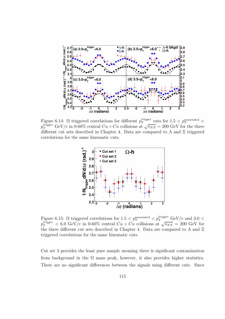
-3 -2 -1 0 1 2 3

-1

(ra

d.)

φ∆

dN

/dtr

igg

er

1/N 2.1

2.2

2.3

2.4

2.5

2.6

2.7 <6.0trigger

T(a) 2.0<p -hΛ

-hΞ

-3 -2 -1 0 1 2 3

2.3

2.4

2.5

2.6

2.7

2.8

2.9<6.0trigger

T(b) 2.5<p -h bkgdΛ

-hΩ

(radians)φ∆-3 -2 -1 0 1 2 3

-1

(ra

d.)

φ∆

dN

/dtr

igg

er

1/N 2.3

2.4

2.5

2.6

2.7

2.8

2.9

3 <6.0trigger

T(c) 3.0<p

(radians)φ∆-3 -2 -1 0 1 2 3

2.22.32.42.52.62.72.82.933.1

<6.0trigger

T(d) 3.5<p

Figure 6.14: Ω triggered correlations for different ptriggerT cuts for 1.5 < passociated

T <ptrigger

T GeV/c in 0-60% central Cu+Cu collisions at√sNN = 200 GeV for the three

different cut sets described in Chapter 4. Data are compared to Λ and Ξ triggeredcorrelations for the same kinematic cuts.

(radians)φ∆-3 -2 -1 0 1 2 3

-1 (

rad

.)φ

∆d

N/d

trig

ge

r1

/N

2.3

2.4

2.5

2.6

2.7

2.8

2.9

3 Cut set 1

Cut set 2

Cut set 3

-hΩ

Figure 6.15: Ω triggered correlations for 1.5 < passociatedT < ptrigger

T GeV/c and 3.0 <ptrigger

T < 6.0 GeV/c in 0-60% central Cu + Cu collisions at√sNN = 200 GeV for

the three different cut sets described in Chapter 4. Data are compared to Λ and Ξtriggered correlations for the same kinematic cuts.

Cut set 3 provides the least pure sample meaning there is significant contamination

from background in the Ω mass peak, however, it also provides higher statistics.

There are no significant differences between the signals using different cuts. Since

115

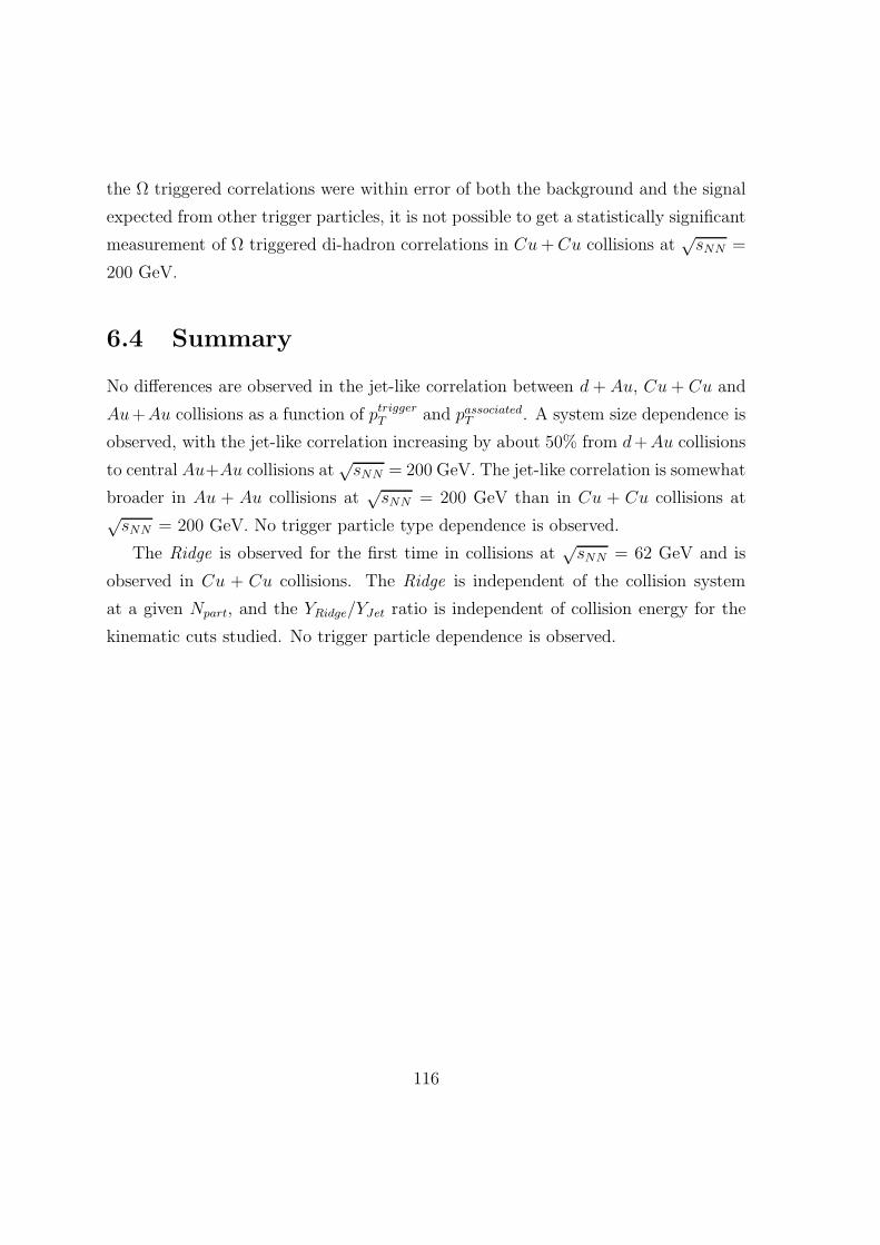
the Ω triggered correlations were within error of both the background and the signal

expected from other trigger particles, it is not possible to get a statistically significant

measurement of Ω triggered di-hadron correlations in Cu+Cu collisions at√sNN =

200 GeV.

6.4 Summary

No differences are observed in the jet-like correlation between d+ Au, Cu+ Cu and

Au+Au collisions as a function of ptriggerT and passociated

T . A system size dependence is

observed, with the jet-like correlation increasing by about 50% from d+Au collisions

to central Au+Au collisions at√sNN = 200 GeV. The jet-like correlation is somewhat

broader in Au + Au collisions at√sNN = 200 GeV than in Cu + Cu collisions at

√sNN = 200 GeV. No trigger particle type dependence is observed.

The Ridge is observed for the first time in collisions at√sNN = 62 GeV and is

observed in Cu + Cu collisions. The Ridge is independent of the collision system

at a given Npart, and the YRidge/YJet ratio is independent of collision energy for the

kinematic cuts studied. No trigger particle dependence is observed.

116

Chapter 7

Discussion

7.1 The jet-like correlation

Various different measurements indicate that the jet-like correlation is dominantly

produced by vacuum fragmentation. The spectra of particles in the jet-like correlation

shown in Figure 2.9 demonstrated behavior suggesting that the jet-like correlation is

dominated by fragmentation. For instance, the spectra of particles in the jet-like

correlation have shallower slopes than the inclusive spectra and become shallower the

higher the momentum of the trigger particle. Likewise, the minimal dependence of

the jet-like yield on the angle relative to the reaction plane shown in Figure 2.12

and the agreement between the di-hadron fragmentation functions in d + Au and

Au+Au shown in Figure 2.10 also suggest that the jet-like correlation is dominantly

produced by fragmentation. The lack of trigger particle dependence demonstrated

in Figure 6.5, Figure 6.6, and Figure 6.7 is expected if the jet-like correlation were

dominated by fragmentation, however, strange particle production in jets is still not

understood well enough to draw strong conclusions on this basis.

The particle composition of the jet-like correlation further indicates that this

feature is dominantly produced by fragmentation. Particle ratios in p + p collisions

at high pT are likely to be dominated by fragmentation. Figure 2.11 demonstrated

that the baryon to meson ratio in the jet-like correlation in central Au+Au collisions

is comparable to that in p + p collisions for both strange and non-strange particles;

117

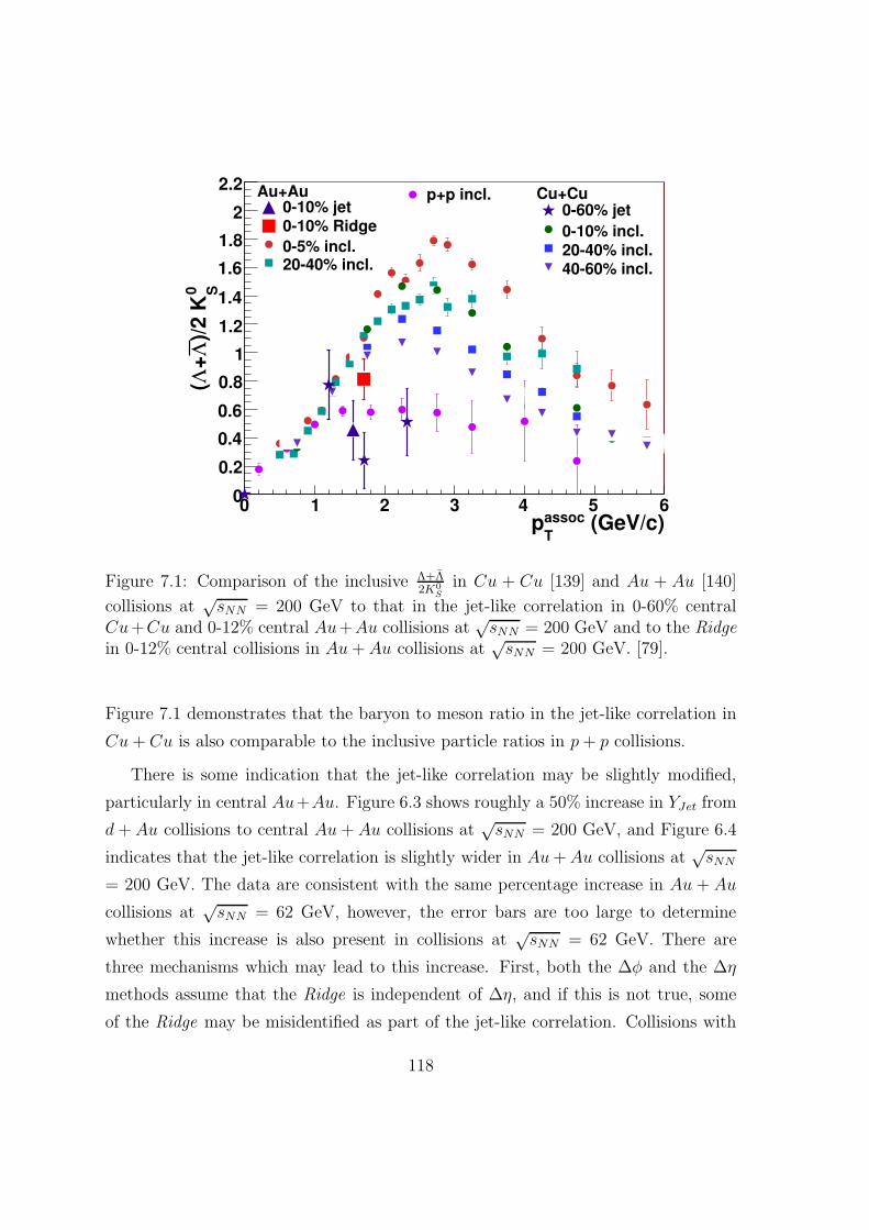
(GeV/c)assoc

Tp

0 1 2 3 4 5 6

S0)/

2 K

Λ+

Λ(

0

0.2

0.4

0.6

0.8

1

1.2

1.4

1.6

1.8

2

2.2 Au+Au0-10% jet0-10% Ridge

0-5% incl.20-40% incl.

Cu+Cu0-60% jet

0-10% incl.20-40% incl.40-60% incl.

p+p incl.

Figure 7.1: Comparison of the inclusive Λ+Λ2K0

S

in Cu + Cu [139] and Au + Au [140]

collisions at√sNN = 200 GeV to that in the jet-like correlation in 0-60% central

Cu+Cu and 0-12% central Au+Au collisions at√sNN = 200 GeV and to the Ridge

in 0-12% central collisions in Au+ Au collisions at√sNN = 200 GeV. [79].

Figure 7.1 demonstrates that the baryon to meson ratio in the jet-like correlation in

Cu+ Cu is also comparable to the inclusive particle ratios in p+ p collisions.

There is some indication that the jet-like correlation may be slightly modified,

particularly in central Au+Au. Figure 6.3 shows roughly a 50% increase in YJet from

d + Au collisions to central Au+ Au collisions at√sNN = 200 GeV, and Figure 6.4

indicates that the jet-like correlation is slightly wider in Au+Au collisions at√sNN

= 200 GeV. The data are consistent with the same percentage increase in Au + Au

collisions at√sNN = 62 GeV, however, the error bars are too large to determine

whether this increase is also present in collisions at√sNN = 62 GeV. There are

three mechanisms which may lead to this increase. First, both the ∆φ and the ∆η

methods assume that the Ridge is independent of ∆η, and if this is not true, some

of the Ridge may be misidentified as part of the jet-like correlation. Collisions with

118

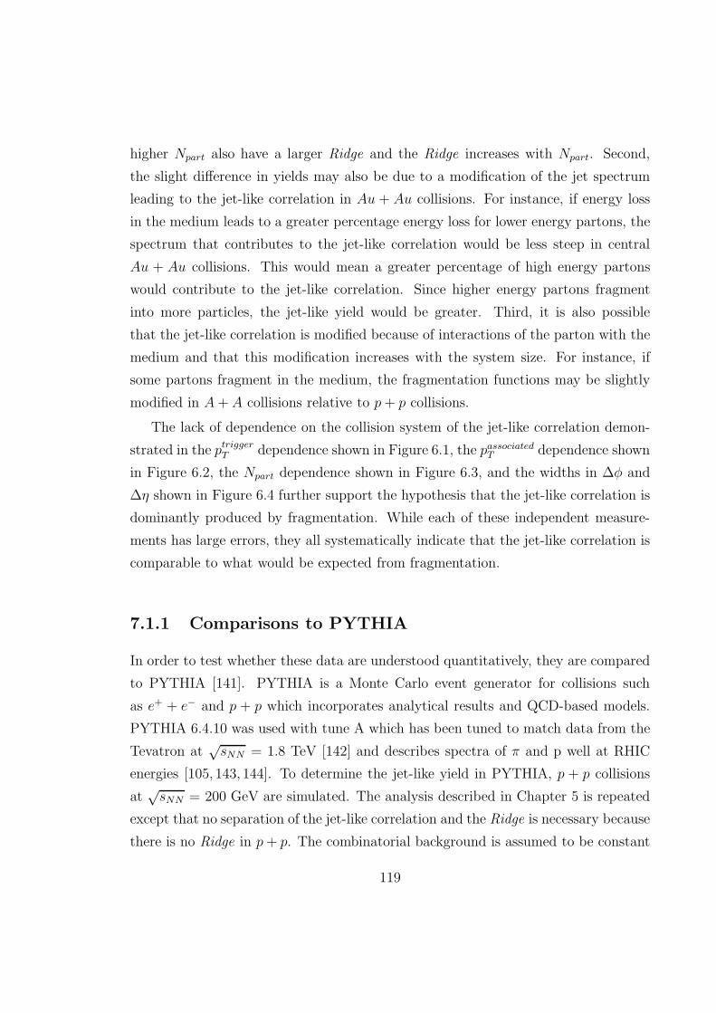
higher Npart also have a larger Ridge and the Ridge increases with Npart. Second,

the slight difference in yields may also be due to a modification of the jet spectrum

leading to the jet-like correlation in Au + Au collisions. For instance, if energy loss

in the medium leads to a greater percentage energy loss for lower energy partons, the

spectrum that contributes to the jet-like correlation would be less steep in central

Au + Au collisions. This would mean a greater percentage of high energy partons

would contribute to the jet-like correlation. Since higher energy partons fragment

into more particles, the jet-like yield would be greater. Third, it is also possible

that the jet-like correlation is modified because of interactions of the parton with the

medium and that this modification increases with the system size. For instance, if

some partons fragment in the medium, the fragmentation functions may be slightly

modified in A+ A collisions relative to p+ p collisions.

The lack of dependence on the collision system of the jet-like correlation demon-

strated in the ptriggerT dependence shown in Figure 6.1, the passociated

T dependence shown

in Figure 6.2, the Npart dependence shown in Figure 6.3, and the widths in ∆φ and

∆η shown in Figure 6.4 further support the hypothesis that the jet-like correlation is

dominantly produced by fragmentation. While each of these independent measure-

ments has large errors, they all systematically indicate that the jet-like correlation is

comparable to what would be expected from fragmentation.

7.1.1 Comparisons to PYTHIA

In order to test whether these data are understood quantitatively, they are compared

to PYTHIA [141]. PYTHIA is a Monte Carlo event generator for collisions such

as e+ + e− and p + p which incorporates analytical results and QCD-based models.

PYTHIA 6.4.10 was used with tune A which has been tuned to match data from the

Tevatron at√sNN = 1.8 TeV [142] and describes spectra of π and p well at RHIC

energies [105, 143, 144]. To determine the jet-like yield in PYTHIA, p + p collisions

at√sNN = 200 GeV are simulated. The analysis described in Chapter 5 is repeated

except that no separation of the jet-like correlation and the Ridge is necessary because

there is no Ridge in p+ p. The combinatorial background is assumed to be constant

119

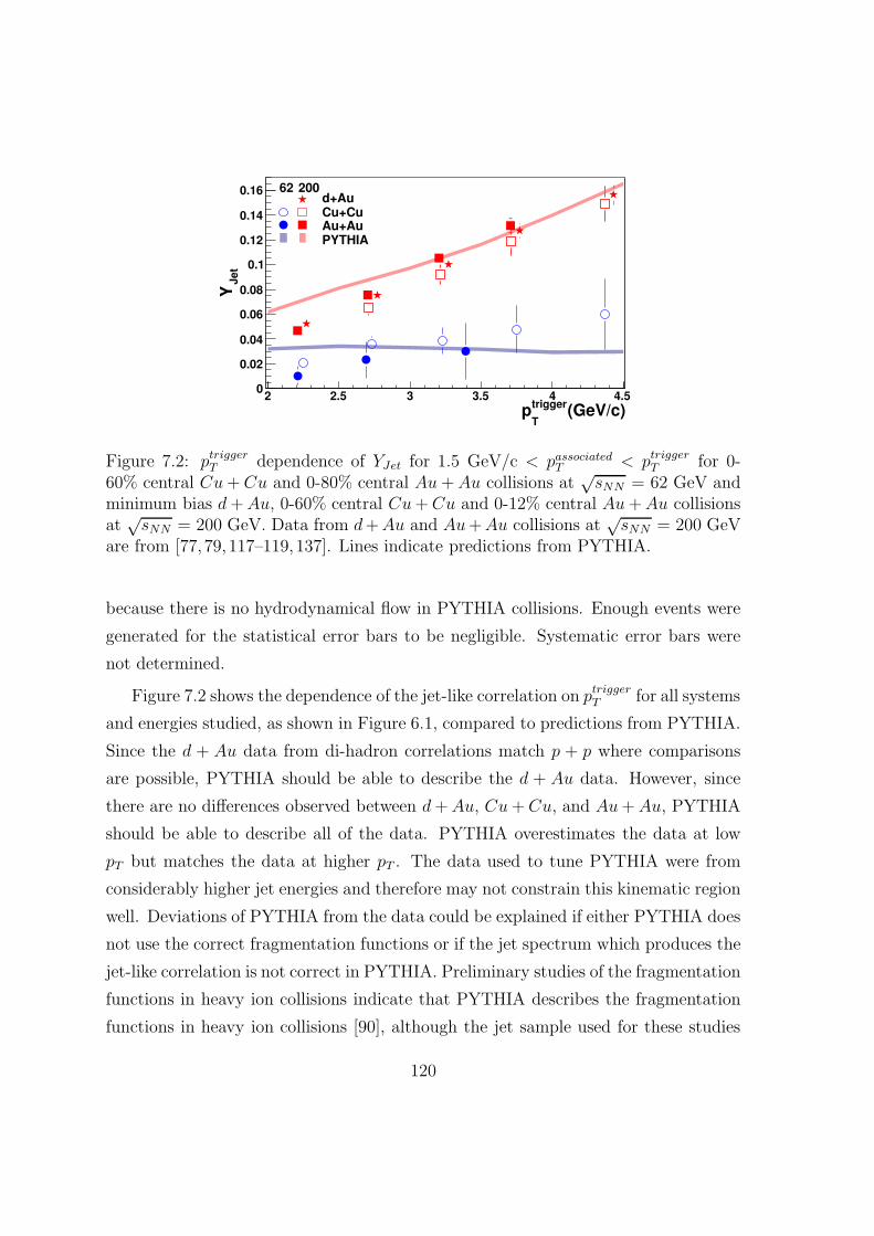
(GeV/c)trigger

Tp

2 2.5 3 3.5 4 4.5

Jet

Y

0

0.02

0.04

0.06

0.08

0.1

0.12

0.14

0.16 62

200

d+AuCu+CuAu+AuPYTHIA

Figure 7.2: ptriggerT dependence of YJet for 1.5 GeV/c < passociated

T < ptriggerT for 0-

60% central Cu+ Cu and 0-80% central Au+Au collisions at√sNN = 62 GeV and

minimum bias d+Au, 0-60% central Cu+Cu and 0-12% central Au+Au collisionsat

√sNN = 200 GeV. Data from d+Au and Au+Au collisions at

√sNN = 200 GeV

are from [77,79, 117–119,137]. Lines indicate predictions from PYTHIA.

because there is no hydrodynamical flow in PYTHIA collisions. Enough events were

generated for the statistical error bars to be negligible. Systematic error bars were

not determined.

Figure 7.2 shows the dependence of the jet-like correlation on ptriggerT for all systems

and energies studied, as shown in Figure 6.1, compared to predictions from PYTHIA.

Since the d + Au data from di-hadron correlations match p + p where comparisons

are possible, PYTHIA should be able to describe the d + Au data. However, since

there are no differences observed between d+Au, Cu+Cu, and Au+Au, PYTHIA

should be able to describe all of the data. PYTHIA overestimates the data at low

pT but matches the data at higher pT . The data used to tune PYTHIA were from

considerably higher jet energies and therefore may not constrain this kinematic region

well. Deviations of PYTHIA from the data could be explained if either PYTHIA does

not use the correct fragmentation functions or if the jet spectrum which produces the

jet-like correlation is not correct in PYTHIA. Preliminary studies of the fragmentation

functions in heavy ion collisions indicate that PYTHIA describes the fragmentation

functions in heavy ion collisions [90], although the jet sample used for these studies

120

(GeV/c)associated

Tp

1 1.5 2 2.5 3

-2 (

Ge

V/c

)T

/dp

Jet

dY

T1

/p

-410

-310

-210

-110

1

62

200

d+AuCu+CuAu+AuPYTHIA 6.4

Figure 7.3: passociatedT dependence of YJet for 1.5 GeV/c < passociated

T < ptriggerT for 3.0 <

ptriggerT < 6.0 GeV/c for 0-60% central Cu+Cu and 0-80% central Au+Au collisions

at√sNN = 62 GeV and minimum bias d + Au, 0-60% central Cu + Cu and 0-12%

central Au + Au collisions at√sNN = 200 GeV. Data from d + Au and Au + Au

collisions at√sNN = 200 GeV are from [77, 79, 117–119, 137]. The lines that match

the data indicate fits, as shown in Figure 7.3, and the thicker, shaded lines indicatepredictions from PYTHIA.

may be biased towards unmodified jets and the average jet energy which leads to the

jet-like correlation presented in Figure 7.2 is considerably lower.

Figure 7.3 shows the dependence of the jet-like yield on passociatedT , as shown in

Figure 6.2, compared to PYTHIA. PYTHIA does not correctly describe the spectrum

of particles in the jet-like correlation in collisions.

The jet-like yield expected in PYTHIA is compared to the data in Figure 6.3 in

Figure 7.4. PYTHIA describes the data in this kinematic range well. The widths in

∆φ and ∆η shown in Figure 6.4 are compared to PYTHIA in Figure 7.5. PYTHIA

underestimates the widths in ∆φ, particularly for the lowest ptriggerT . While the d+Au

data are higher than PYTHIA, the widths in A + A are larger than d + Au and the

width grows with Npart. The widths in ∆η generally agree with the data except for

the lowest passociatedT in Cu + Cu collisions and for the lowest ptrigger

T in Au + Au

collisions at√sNN = 200 GeV. The width in ∆η in Au + Au collisions at

√sNN =

200 GeV matches PYTHIA in the most peripheral collisions but by the most central

121

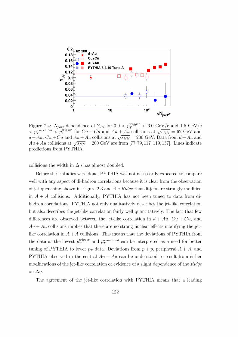
>part<N1 10 210

Jet

Y

0

0.02

0.04

0.06

0.08

0.1

0.12

0.14

0.16

0.18

0.262

200

d+Au

Cu+Cu

Au+Au

PYTHIA 6.4.10 Tune A

Figure 7.4: Npart dependence of YJet for 3.0 < ptriggerT < 6.0 GeV/c and 1.5 GeV/c

< passociatedT < ptrigger

T for Cu + Cu and Au + Au collisions at√sNN = 62 GeV and

d+Au, Cu+Cu and Au+Au collisions at√sNN = 200 GeV. Data from d+Au and

Au+Au collisions at√sNN = 200 GeV are from [77,79,117–119,137]. Lines indicate

predictions from PYTHIA.

collisions the width in ∆η has almost doubled.

Before these studies were done, PYTHIA was not necessarily expected to compare

well with any aspect of di-hadron correlations because it is clear from the observation

of jet quenching shown in Figure 2.3 and the Ridge that di-jets are strongly modified

in A + A collisions. Additionally, PYTHIA has not been tuned to data from di-

hadron correlations. PYTHIA not only qualitatively describes the jet-like correlation

but also describes the jet-like correlation fairly well quantitatively. The fact that few

differences are observed between the jet-like correlation in d + Au, Cu + Cu, and

Au+Au collisions implies that there are no strong nuclear effects modifying the jet-

like correlation in A+A collisions. This means that the deviations of PYTHIA from

the data at the lowest ptriggerT and passociated

T can be interpreted as a need for better

tuning of PYTHIA to lower pT data. Deviations from p + p, peripheral A + A, and

PYTHIA observed in the central Au + Au can be understood to result from either

modifications of the jet-like correlation or evidence of a slight dependence of the Ridge

on ∆η.

The agreement of the jet-like correlation with PYTHIA means that a leading

122

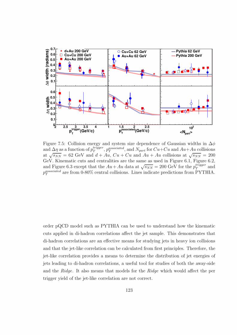
2 2.5 3 3.5 4 4.5

wid

th (

rad

ian

s)

φ∆

0

0.1

0.2

0.3

0.4

0.5

0.6

0.7d+Au 200 GeVCu+Cu 200 GeVAu+Au 200 GeV

1 1.5 2 2.5 3

Cu+Cu 62 GeVAu+Au 62 GeV

0

0.1

0.2

0.3

0.4

0.5

0.6

0.7Pythia 62 GeV

Pythia 200 GeV

(GeV/c)trigger

Tp

2 2.5 3 3.5 4 4.5

wid

thη

∆

0

0.1

0.2

0.3

0.4

0.5

0.6

0.7

(GeV/c)associated

Tp

1 1.5 2 2.5 3

>part<N

210

0

0.1

0.2

0.3

0.4

0.5

0.6

0.7

Figure 7.5: Collision energy and system size dependence of Gaussian widths in ∆φand ∆η as a function of ptrigger

T , passociatedT , andNpart for Cu+Cu and Au+Au collisions

at√sNN = 62 GeV and d + Au, Cu + Cu and Au + Au collisions at

√sNN = 200

GeV. Kinematic cuts and centralities are the same as used in Figure 6.1, Figure 6.2,and Figure 6.3 except that the Au+Au data at

√sNN = 200 GeV for the ptrigger

T andpassociated

T are from 0-80% central collisions. Lines indicate predictions from PYTHIA.

order pQCD model such as PYTHIA can be used to understand how the kinematic

cuts applied in di-hadron correlations affect the jet sample. This demonstrates that

di-hadron correlations are an effective means for studying jets in heavy ion collisions

and that the jet-like correlation can be calculated from first principles. Therefore, the

jet-like correlation provides a means to determine the distribution of jet energies of

jets leading to di-hadron correlations, a useful tool for studies of both the away-side

and the Ridge. It also means that models for the Ridge which would affect the per

trigger yield of the jet-like correlation are not correct.

123

Figure 7.6: Schematic diagram depicting the radial flow plus trigger bias model

7.2 The Ridge

7.2.1 Theoretical descriptions of the Ridge

The Ridge is a novel feature only observed in heavy ion collisions. Multiple differ-

ent models have been proposed to explain the Ridge. These models build on the

theoretical frameworks used to describe heavy ion collisions discussed in Chapter 1.

Radial flow plus trigger bias

The radial flow plus trigger bias model explains the Ridge as an incidental rather

than a causal correlation between particles [145]. As discussed in Chapter 1, there is

evidence that the medium produced in central heavy ion collisions at RHIC can be

described as a fluid and that there are pressure gradients in this fluid. Hydrodynam-

ical models predict the expansion of the medium through radial flow, meaning that

particles in the bulk get a radial velocity boost so that they are mostly emitted per-

pendicular to the surface of the medium. In the radial flow plus trigger bias model,

hard partons are also emitted mostly perpendicular to the surface of the medium.

The hard partons may either get a radial velocity boost from radial flow, or they

may be surface-biased jets. Either mechanism means that both the particles from

the jet and particles from the medium come mostly from the surface, resulting in

124

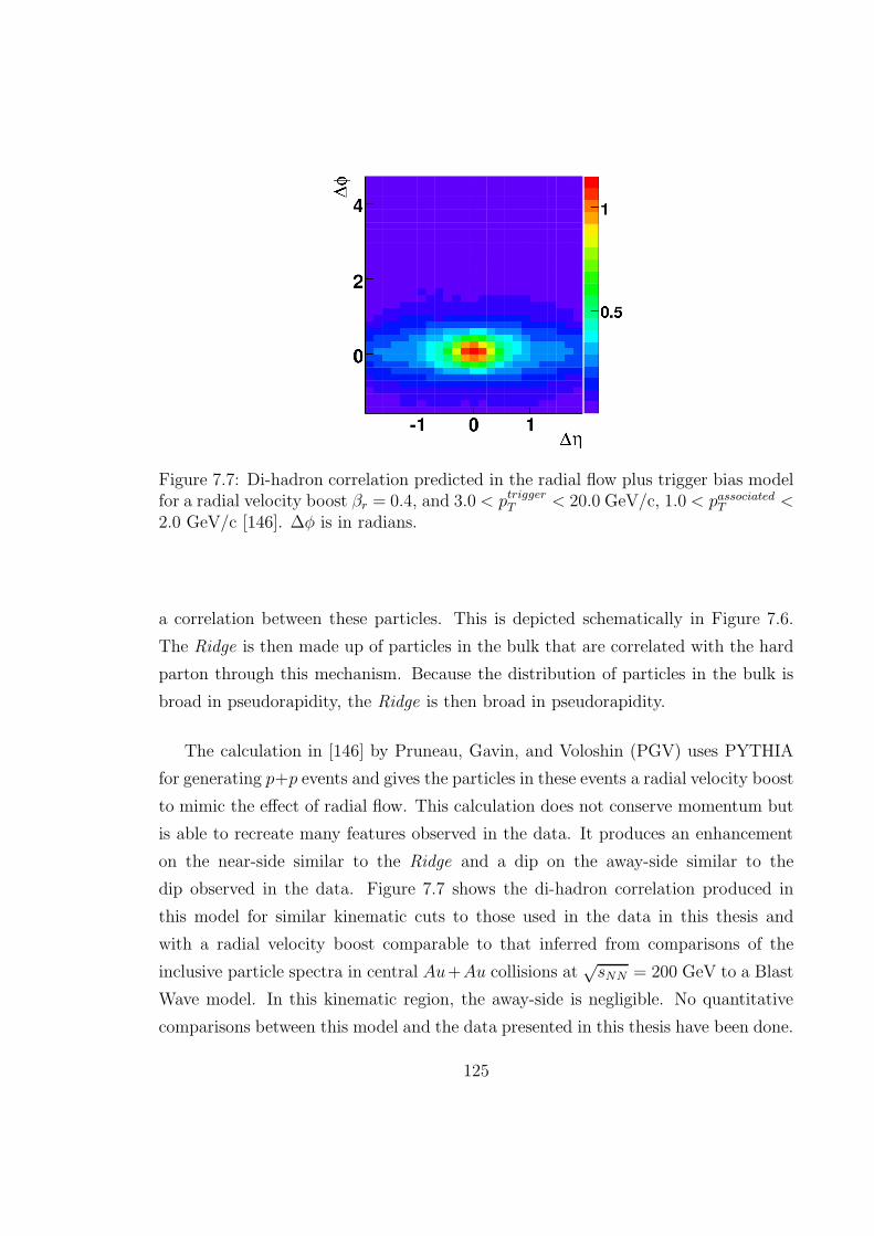
Figure 7.7: Di-hadron correlation predicted in the radial flow plus trigger bias modelfor a radial velocity boost βr = 0.4, and 3.0 < ptrigger

T < 20.0 GeV/c, 1.0 < passociatedT <

2.0 GeV/c [146]. ∆φ is in radians.

a correlation between these particles. This is depicted schematically in Figure 7.6.

The Ridge is then made up of particles in the bulk that are correlated with the hard

parton through this mechanism. Because the distribution of particles in the bulk is

broad in pseudorapidity, the Ridge is then broad in pseudorapidity.

The calculation in [146] by Pruneau, Gavin, and Voloshin (PGV) uses PYTHIA

for generating p+p events and gives the particles in these events a radial velocity boost

to mimic the effect of radial flow. This calculation does not conserve momentum but

is able to recreate many features observed in the data. It produces an enhancement

on the near-side similar to the Ridge and a dip on the away-side similar to the

dip observed in the data. Figure 7.7 shows the di-hadron correlation produced in

this model for similar kinematic cuts to those used in the data in this thesis and

with a radial velocity boost comparable to that inferred from comparisons of the

inclusive particle spectra in central Au+Au collisions at√sNN = 200 GeV to a Blast

Wave model. In this kinematic region, the away-side is negligible. No quantitative

comparisons between this model and the data presented in this thesis have been done.

125

η∆

-6

-4

-2

0

2

4

6

φ∆ -3-2

-10

12

3

η

∆ dφ

∆d

N2

d

trig

gN

1

0

0.2

0.4

0.6

0.8

1

Figure 7.8: Di-hadron correlation predicted for 2.5 GeV/c < ptriggerT and 1.0 GeV/c

< passociatedT in [147]. ∆φ is in radians.

Theoretical calculations involving both jets and hydrodynamics are difficult be-

cause hydrodynamics inherently describes processes that occur in a fluid at equilib-

rium and jets are inherently not at equilibrium. Attempts to calculate the production

of the Ridge through the radial flow plus trigger bias mechanism using a hydrody-

namical framework have been done, although they do not yet agree with the data.

This may be due to the inherent difficulty in such calculations. The calculation by

Shuryak in [148] gets the width of the Ridge in azimuth a factor of two larger than

observed in the data. The calculation in [147] by Takahashi et al is a full 3D hydro-

dynamical calculation which reproduces many of the general features in the data, as

shown in Figure 7.8. In this calculation a hard parton is mimicked by introducing

hot cells into the hydrodynamical calculation. In addition to producing a Ridge, this

leaves a correlation which looks like the jet-like correlation, even though there are no

jets generated.

Glasma flux tubes

In the Color Glass Condensate (CGC) picture, the incoming nuclei are described as

two sheets of Glasma. When these sheets collide, strong color magnetic and electric

126

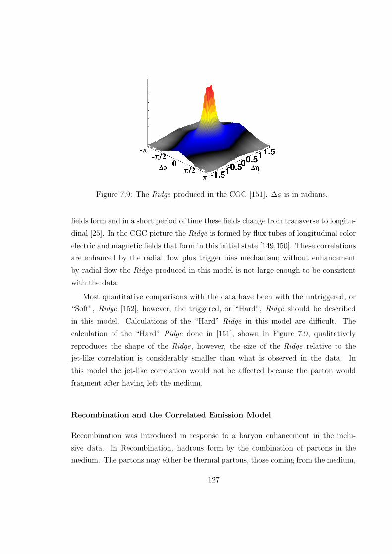
Figure 7.9: The Ridge produced in the CGC [151]. ∆φ is in radians.

fields form and in a short period of time these fields change from transverse to longitu-

dinal [25]. In the CGC picture the Ridge is formed by flux tubes of longitudinal color

electric and magnetic fields that form in this initial state [149,150]. These correlations

are enhanced by the radial flow plus trigger bias mechanism; without enhancement

by radial flow the Ridge produced in this model is not large enough to be consistent

with the data.

Most quantitative comparisons with the data have been with the untriggered, or

“Soft”, Ridge [152], however, the triggered, or “Hard”, Ridge should be described

in this model. Calculations of the “Hard” Ridge in this model are difficult. The

calculation of the “Hard” Ridge done in [151], shown in Figure 7.9, qualitatively

reproduces the shape of the Ridge, however, the size of the Ridge relative to the

jet-like correlation is considerably smaller than what is observed in the data. In

this model the jet-like correlation would not be affected because the parton would

fragment after having left the medium.

Recombination and the Correlated Emission Model

Recombination was introduced in response to a baryon enhancement in the inclu-

sive data. In Recombination, hadrons form by the combination of partons in the

medium. The partons may either be thermal partons, those coming from the medium,

127

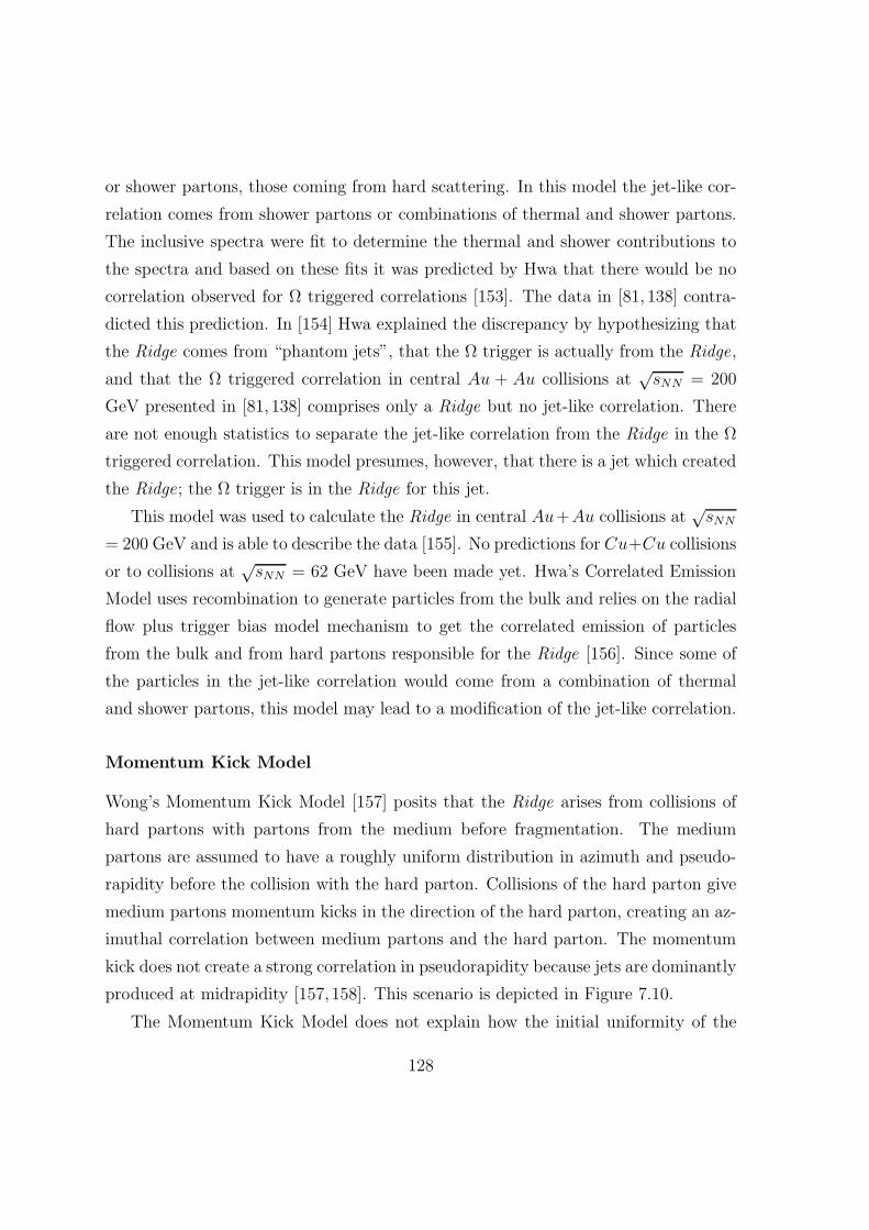
or shower partons, those coming from hard scattering. In this model the jet-like cor-

relation comes from shower partons or combinations of thermal and shower partons.

The inclusive spectra were fit to determine the thermal and shower contributions to

the spectra and based on these fits it was predicted by Hwa that there would be no

correlation observed for Ω triggered correlations [153]. The data in [81, 138] contra-

dicted this prediction. In [154] Hwa explained the discrepancy by hypothesizing that

the Ridge comes from “phantom jets”, that the Ω trigger is actually from the Ridge,

and that the Ω triggered correlation in central Au + Au collisions at√sNN = 200

GeV presented in [81, 138] comprises only a Ridge but no jet-like correlation. There

are not enough statistics to separate the jet-like correlation from the Ridge in the Ω

triggered correlation. This model presumes, however, that there is a jet which created

the Ridge; the Ω trigger is in the Ridge for this jet.

This model was used to calculate the Ridge in central Au+Au collisions at√sNN

= 200 GeV and is able to describe the data [155]. No predictions for Cu+Cu collisions

or to collisions at√sNN = 62 GeV have been made yet. Hwa’s Correlated Emission

Model uses recombination to generate particles from the bulk and relies on the radial

flow plus trigger bias model mechanism to get the correlated emission of particles

from the bulk and from hard partons responsible for the Ridge [156]. Since some of

the particles in the jet-like correlation would come from a combination of thermal

and shower partons, this model may lead to a modification of the jet-like correlation.

Momentum Kick Model

Wong’s Momentum Kick Model [157] posits that the Ridge arises from collisions of

hard partons with partons from the medium before fragmentation. The medium

partons are assumed to have a roughly uniform distribution in azimuth and pseudo-

rapidity before the collision with the hard parton. Collisions of the hard parton give

medium partons momentum kicks in the direction of the hard parton, creating an az-

imuthal correlation between medium partons and the hard parton. The momentum

kick does not create a strong correlation in pseudorapidity because jets are dominantly

produced at midrapidity [157, 158]. This scenario is depicted in Figure 7.10.

The Momentum Kick Model does not explain how the initial uniformity of the

128

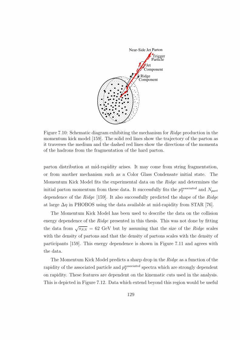
Ridge

JetComponent

Component

Near-Side Jet Parton

TriggerParticle

Figure 7.10: Schematic diagram exhibiting the mechanism for Ridge production in themomentum kick model [159]. The solid red lines show the trajectory of the parton asit traverses the medium and the dashed red lines show the directions of the momentaof the hadrons from the fragmentation of the hard parton.

parton distribution at mid-rapidity arises. It may come from string fragmentation,

or from another mechanism such as a Color Glass Condensate initial state. The

Momentum Kick Model fits the experimental data on the Ridge and determines the

initial parton momentum from these data. It successfully fits the passociatedT and Npart

dependence of the Ridge [159]. It also successfully predicted the shape of the Ridge

at large ∆η in PHOBOS using the data available at mid-rapidity from STAR [76].

The Momentum Kick Model has been used to describe the data on the collision

energy dependence of the Ridge presented in this thesis. This was not done by fitting

the data from√sNN = 62 GeV but by assuming that the size of the Ridge scales

with the density of partons and that the density of partons scales with the density of

participants [159]. This energy dependence is shown in Figure 7.11 and agrees with

the data.

The Momentum Kick Model predicts a sharp drop in the Ridge as a function of the

rapidity of the associated particle and passociatedT spectra which are strongly dependent

on rapidity. These features are dependent on the kinematic cuts used in the analysis.

This is depicted in Figure 7.12. Data which extend beyond this region would be useful

129

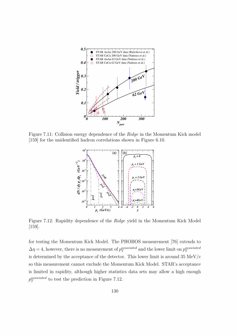
0 100 200 300N

part

0

0.1

0.2

0.3

0.4

0.5

Yie

ld /

tri

gger

STAR AuAu 200 GeV data (Bielcikova et al.)

STAR CuCu 200 GeV data (Nattrass et al.)

STAR AuAu 62 GeV data (Nattrass et al.)

STAR CuCu 62 GeV data (Nattrass et al.)

200 GeV

62 GeV

Figure 7.11: Collision energy dependence of the Ridge in the Momentum Kick model[159] for the unidentified hadron correlations shown in Figure 6.10.

0 1 2 3 4

pt (GeV/c)

10-4

10-3

10-2

10-1

100

101

dN

/ d

y p

t dp

t (

GeV

-2)

-6 -4 -2 0 2 4 6

y

(a) (b)

y=0

y=1

pt = 0

y=2

y=3y=

4

pt = 1 GeV

pt = 2 GeV

pt=3GeV

pt=4GeV

Figure 7.12: Rapidity dependence of the Ridge yield in the Momentum Kick Model[159].

for testing the Momentum Kick Model. The PHOBOS measurement [76] extends to

∆η = 4, however, there is no measurement of passociatedT and the lower limit on passociated

T

is determined by the acceptance of the detector. This lower limit is around 35 MeV/c

so this measurement cannot exclude the Momentum Kick Model. STAR’s acceptance

is limited in rapidity, although higher statistics data sets may allow a high enough

passociatedT to test the prediction in Figure 7.12.

130

Figure 7.13: Ridge production through radiated gluons broadened by transverse flow[65]

Bremsstrahlung gluons broadened by medium interactions

The hard partons which fragment into jets may emit bremsstrahlung gluons. It is

hypothesized in [65] that the Ridge is the result of gluon bremsstrahlung in the

medium broadened by transverse flow, as depicted schematically in Figure 7.13. This

model describes moderate broadening of the jet-like correlation in ∆η, however, it has

difficulty with producing a structure as broad in ∆η as the Ridge. The calculations

in [65] predict a Ridge which is only about 10% broader in ∆η than the jet-like

correlation.

The formation of the Ridge from bremsstrahlung gluons is also hypothesized in

[160], however, in this model the gluons are broadened by strong, turbulent color

fields. These strong color fields are predicted to be produced in response to plasma

instabilities. If such fields exist, they would deflect brehmstralung gluons. Figure 7.14

shows the broadening predicted in [160] for two different jet energies; the structure

in these figures is not broad enough to be consistent with the data.

7.2.2 Discussion

Data on the Ridge is extensive and there are several observations which may be key

to distinguishing production mechanisms for the Ridge:

131

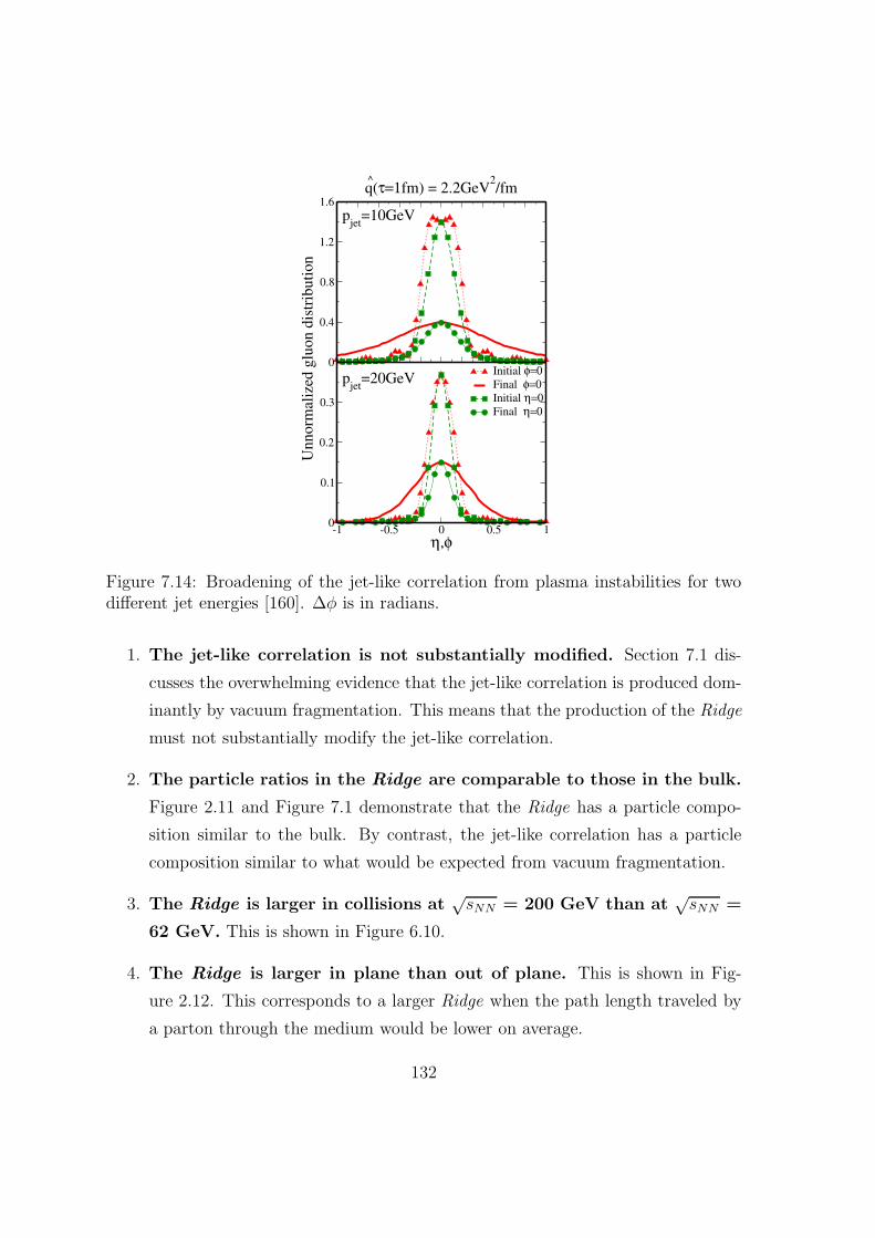
0

0.4

0.8

1.2

1.6

^q(τ=1fm) = 2.2GeV

2/fm

-1 -0.5 0 0.5 1

η,φ

0

0.1

0.2

0.3

Un

no

rmal

ized

glu

on

dis

trib

uti

on

Initial φ=0

Final φ=0

Initial η=0

Final η=0

pjet

=10GeV

pjet

=20GeV

Figure 7.14: Broadening of the jet-like correlation from plasma instabilities for twodifferent jet energies [160]. ∆φ is in radians.

1. The jet-like correlation is not substantially modified. Section 7.1 dis-

cusses the overwhelming evidence that the jet-like correlation is produced dom-

inantly by vacuum fragmentation. This means that the production of the Ridge

must not substantially modify the jet-like correlation.

2. The particle ratios in the Ridge are comparable to those in the bulk.

Figure 2.11 and Figure 7.1 demonstrate that the Ridge has a particle compo-

sition similar to the bulk. By contrast, the jet-like correlation has a particle

composition similar to what would be expected from vacuum fragmentation.

3. The Ridge is larger in collisions at√sNN = 200 GeV than at

√sNN =

62 GeV. This is shown in Figure 6.10.

4. The Ridge is larger in plane than out of plane. This is shown in Fig-

ure 2.12. This corresponds to a larger Ridge when the path length traveled by

a parton through the medium would be lower on average.

132

5. There is either no dependence on the trigger particle or a larger Ridge

for a heavier trigger particle. Figure 6.12 shows the dependence of the Ridge

on Npart for different trigger particle species. It is unclear how correlated the

systematic errors due to v2 are so it is difficult to conclusively say that there

is mass dependence. However, if the systematic errors are correlated, then the

Ridge is larger for Λ trigger particles than for unidentified trigger particles and

it is smaller for K0S trigger particles than for an unidentified trigger particles.

Figure 2.11 shows that in the kinematic range of the trigger particle there

are roughly as many protons as pions. Since protons and pions are the most

abundant particles, this means that the unidentified hadron trigger particles

are roughly 50% protons and roughly 50% pions, making the average mass

for unidentified triggers between the Λ mass and the K0S mass. This means

that if the systematic errors in Figure 6.12 are correlated, the Ridge is larger

for heavier trigger particles. A smaller Ridge for heavier trigger particles is

strongly disfavored by the data.

6. The Ridge is broad in ∆η. The Ridge is roughly independent of ∆η within

the STAR acceptance. There is some room for a slight ∆η dependence, but

there cannot be a strong dependence on ∆η. The PHOBOS measurement [76]

demonstrated that the Ridge extends to ∆η = 4, however, the associated par-

ticles were determined from single hits, so the kinematic reach was limited by

the acceptance of the detector. This limit is about pT > 35 MeV/c. The extent

of the Ridge may cause some problems for causal models because a parton at

midrapidity has to affect particles separated by a large gap in ∆η.

Radial flow plus trigger bias mechanism and related models

The Glasma Flux Tube model and the Correlated Emission Model both primarily

produce the Ridge using the radial flow plus trigger bias mechanism. The radial

flow plus trigger bias mechanism naturally leads to agreement with many of the

experimental observations. Because hard partons fragment as in a vacuum in the

PGV and Shuryak calculations, these models do not modify the jet-like correlation,

133

in agreement with observation 1. The Recombination model by Hwa may lead to

some modification of the jet-like correlation because some of the jet-like correlation

could come from recombination of shower and thermal partons rather than vacuum

fragmentation. A calculation needs to be done in this framework to ensure that the

Recombination model is consistent with observation 1. In all models, particles in

the Ridge come from the bulk, in agreement with observation 2. Assuming that the

reaction plane dependence calculated in the Correlated Emission Model [156] is a

common feature of the radial flow plus trigger bias mechanism, these models are also

in agreement with observation 4. The Ridge would also be expected to have roughly

the same extent in ∆η as inclusive particles, in agreement with observation 6.

It is not clear whether the energy dependence (observation 3) is consistent with

this model but the energy dependence would be readily calculated in the same way

as done by PGV [146]. The amount of radial flow can be determined by comparisons

with the inclusive spectra. As shown in Figure 1.16 for v2, lighter particles are affected

more by hydrodynamical flow. If these models are dependent on a velocity boost for

the surface bias of the hard parton, then a dependence on the mass of the trigger

particle should be observed and lighter trigger particles should correspond to a larger

Ridge. This contradicts observation 5. This means that if the radial flow plus trigger

bias mechanism is the proper mechanism for producing the Ridge, the surface bias of

the hard partons likely does not come from radial flow but from jet quenching.

The Momentum Kick Model

In the Momentum Kick Model the jet-like correlation is produced by vacuum frag-

mentation of the parton after it interacts with the medium. The jet-like correlation

is not affected, in agreement with observation 1. The Ridge is created by medium

partons so naturally has the same composition as the bulk, in agreement with obser-

vation 2. As shown in Figure 7.11, the Momentum Kick Model describes the energy

dependence of the Ridge, in agreement with observation 3. No calculations have been

made for the dependence of the Ridge on trigger particle type, so it is unclear if this

model is consistent with observation 5.

134

Naively the larger path length out of plane would lead to a larger Ridge, in con-

tradiction to observation 4. It may be possible to reconcile this with the data if the

parton loses so much energy when it travels out of plane that it is not observed. In

that case only jets from the surface would be observed out of plane. The reaction

plane dependence of the Ridge in the Momentum Kick Model has not been calculated

yet.

The Momentum Kick Model is the only causal model that produces a Ridge broad

enough to be consistent with the data, in agreement with observation 6. However,

this model also has a sharp drop just outside of reach of current measurements. This

unusual feature, if observed, would be one signature that the Momentum Kick Model

is the correct mechanism for the production of the Ridge.

Gluon Bremsstrahlung Models

In gluon bremsstrahlung models, the hard parton fragments in the vacuum after

having emitted bremsstrahlung gluons, in agreement with observation 1. In these

models, the Ridge would come from the fragmentation of gluons, which would naively

seem to contradict observation 2, that the Ridge composition is similar to the bulk. If

the bremsstrahlung gluons are sufficiently soft that they reinteract with the medium,

this may be able to be reconciled with the data. No calculation of the collision energy

dependence has been done, however, the expectations from these models seem to be

consistent with observation 3. These models seem to have the same contradiction

with observation 4 that the Momentum Kick Model does, that naively the larger

path length out of plane would lead to a larger Ridge. If heavier trigger particles

correspond on average to heavier partons, then lighter trigger particles should produce

a larger Ridge because the amount of bremsstrahlung is proportional to m−4. This is

in contradiction to observation 5. These models also have difficulty producing a Ridge

broad enough in pseudorapidity to match the data, in contradiction to observation 6.

135

7.2.3 Summary

The origin of the Ridge is not yet conclusive. More quantitative theoretical calcula-

tions are needed in order to compare the data with the models. Gluon bremsstrahlung

models are likely excluded by the data because they are apparently in contradiction

with the observations on the reaction plane dependence of the Ridge, the trigger

particle type dependence of the Ridge, and the extent of the Ridge in ∆η. This

does not mean that these mechanisms do not modify hadron fragmentation in heavy

ion collisions, only that they are not likely to be the cause of the Ridge. Indeed,

gluon bremsstrahlung could cause the observed broadening of the jet-like correlation

in central Au+ Au collisions at√sNN = 200 GeV.

The Momentum Kick Model is consistent with the data so far. A calculation of

the reaction plane dependence is crucial to determine if this model is in agreement

with the data. Measurements which would test the prediction of a sharp drop of the

Ridge with ∆η are also crucial.

Models which rely on the radial flow plus trigger bias mechanism qualitatively

agree with the data. More precise calculations are needed. Radial flow plus trigger

bias would be the simplest mechanism to describe the Ridge since hydrodynamics

describes the azimuthal asymmetry of particles produced in heavy ion collisions and

radial flow has been observed in the inclusive spectra of particles. If the radial flow

plus trigger bias model is sufficient to explain the data, there is no need for more

complicated, speculative mechanisms to produce the Ridge. The significance of the

Ridge in such a scenario would be that it would show up as a background in methods

such as jet reconstruction and it is vital to understand how this background would

affect reconstructed jets. It also may be possible to learn something quantitative

about radial flow from the Ridge; more theoretical developments along these lines

would be necessary to determine if this is possible.

136

Chapter 8

Conclusions and outlook

The data in this thesis, combined with the data available from previous studies,

demonstrate that the jet-like correlation is produced dominantly by fragmentation.

These data are described well both qualitatively and quantitatively by PYTHIA,

making the jet-like correlation one of the best understood features in heavy ion col-

lisions. The small deviations of the jet-like correlation in different collision systems

indicate modifications of the jet-like correlation. The jet-like correlation can be used

to determine how kinematic cuts affect the sample of jets leading to di-hadron corre-

lations and can therefore be used as a tool to study both the away-side of di-hadron

correlations and the Ridge.

These studies are in the momentum regime where the baryon to meson ratio

is greatest, as shown in Figure 1.19, which led to the hypothesis that partons do

not hadronize by the same mechanism in A + A collisions as in p + p collisions but

rather hadronized via Recombination. Recombination proposes that the dominant

production for hadrons at intermediate pT (2-6 GeV/c) is by the combination of

quarks from the medium. The data presented here indicate that hadrons at pT ≈ 3

GeV/c in A + A collisions are as likely to be produced from vacuum fragmentation

as hadrons at pT ≈ 3 GeV/c in p + p collisions. If partons hadronize through a

different mechanism in A+A collisions than in p+p collisions, the jet-like correlation

should be affected. A 3 GeV/c hadron formed through Recombination naively would

not have a jet-like correlation associated with it. If there were some combination of

137

Recombination and vacuum, there would be more trigger particles at 3 GeV/c but

the same number of associated particles. This would make the jet-like yield smaller,

the opposite of what is observed in the data. It is not clear how to reconcile these

two pictures.

The interpretation of the Ridge is less conclusive, in large part because theoret-

ical models are still not well developed. There are many proposed mechanisms for

the production of the Ridge, however, so far there are few quantitative comparisons.

Models for the production of the Ridge through partonic energy loss via gluon brehm-

strahlung have difficulty producing a Ridge wide enough in ∆η to be in agreement

with the data. The Momentum Kick Model, a model for the production of the Ridge

through partonic energy loss via collisions, may have difficulty with the reaction plane

dependence. All causal models may have difficulty with the extent of the Ridge in ∆η.

Most non-causal models rely heavily on the same mechanism, radial flow plus trigger

bias, for the production of the Ridge. The radial flow plus trigger bias mechanism

would not require any new speculative mechanisms and these models qualitatively

reproduce many of the features of the data from central Au+Au collisions at√sNN

= 200 GeV. However, none of the calculations to date have been complete enough

to conclusively determine that this is the mechanism that produces the Ridge. If the

Ridge is produced by radial flow plus trigger bias, this would support the description

of the medium as a fluid since it would be another indication of the collective flow

of partons. Further theoretical studies are needed to test these mechanisms and, if

the Ridge is produced by radial flow, to determine if the Ridge can be used to better

understand radial flow.

8.1 Future measurements

8.1.1 Studies at√sNN = 200 GeV

The STAR detector has been upgraded to include a Time of Flight (TOF) detector,

with most of this detector already installed for the 2009 p+ p run. This will provide

138

better particle identification over a wider pT range and therefore improve the mea-

surements of the particle ratios in the Ridge and the jet-like correlations. As shown

in Figure 3.9, particle identification using dE/dx in the TPC is difficult for momenta

greater than 1 GeV/c. Particle identification in the relativistic rise region is only

possible for momenta above 2.5 GeV/c. The TOF is capable of particle identification

in the region that the TPC is not, as shown in the time of flight verses the momentum

as measured by the TOF in the 2009 p + p run in Figure 8.1. This will also aid in

the efficient identification of Ω triggers for future studies since pions misidentified as

kaons make significant contributions to the background of the Ω mass peak. Studies

of the Ridge with higher mass trigger particles could provide crucial tests of the radial

flow plus trigger bias model. In addition, there have been substantial improvements

in the use of the calorimeters in STAR for triggering both on high-pT particles and

on jets. The current luminosity is substantially higher than in the year 4 Au + Au

run. Measurements are currently limited at high-pT by the cross section and the im-

proved triggering capacity of STAR will allow measurements at higher ptriggerT . The

electromagnetic calorimeter can trigger on events with large deposits of energy in the

calorimeter, mostly from electrons, π0 and γ. This will enable studies of whether

there is a Ridge with a direct photon trigger, a measurement which may give insight

into the production mechanism of the Ridge.

The largest development in studies of jets in heavy ion collisions has been jet

reconstruction, as discussed in Chapter 2. Full jet reconstruction allows the determi-

nation of partonic energy and therefore allows more detailed measurements of partonic

energy loss. Di-hadron correlations suffer from the ambiguity of whether or not a jet

was formed and the large combinatorial background in di-hadron correlations comes

from hadrons which were not formed in jets. This ambiguity is not an issue for fully

reconstructed jets. The most obvious question is whether the Ridge is still evident

when a jet is fully reconstructed, a measurement crucial for distinguishing between

causal and non-causal production mechanisms for the Ridge. This measurement can

be done using a reconstructed jet as a trigger and looking at the distribution of

hadrons relative to the jet axis in ∆φ and ∆η.

Whether or not the Ridge should be considered part of the jet depends on whether

139

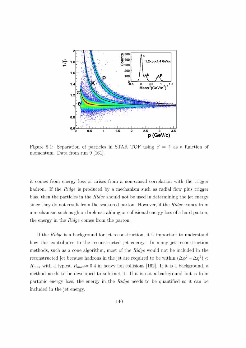
Figure 8.1: Separation of particles in STAR TOF using β = vc

as a function ofmomentum. Data from run 9 [161].

it comes from energy loss or arises from a non-causal correlation with the trigger

hadron. If the Ridge is produced by a mechanism such as radial flow plus trigger

bias, then the particles in the Ridge should not be used in determining the jet energy

since they do not result from the scattered parton. However, if the Ridge comes from

a mechanism such as gluon brehmstrahlung or collisional energy loss of a hard parton,

the energy in the Ridge comes from the parton.

If the Ridge is a background for jet reconstruction, it is important to understand

how this contributes to the reconstructed jet energy. In many jet reconstruction

methods, such as a cone algorithm, most of the Ridge would not be included in the

reconstructed jet because hadrons in the jet are required to be within (∆φ2 +∆η2) <

Rmax with a typical Rmax≈ 0.4 in heavy ion collisions [162]. If it is a background, a

method needs to be developed to subtract it. If it is not a background but is from

partonic energy loss, the energy in the Ridge needs to be quantified so it can be

included in the jet energy.

140

8.1.2 Studies of the energy dependence

Future studies of the collision energy dependence of the Ridge will be possible at both

RHIC and the Large Hadron Collider (LHC). The RHIC program will have a beam

energy scan which will provide Au+Au collisions from√sNN = 5 - 39 GeV in 2010.

The LHC will provide Pb + Pb collisions at 5.5 TeV, with the first heavy ion run

scheduled in 2011.

RHIC beam energy scan

It is unclear theoretically whether or not a Ridge is expected at lower√sNN . If the

Ridge arises from partonic energy loss in the colored medium, it may only be present

above the critical temperature. If the Ridge comes from radial flow plus trigger bias,

there will be a Ridge if the medium is opaque enough to create a surface bias for the

trigger particle and the medium is described well by hydrodynamics.

An estimate of the Ridge yield at lower energies can be made from a straightfor-

ward extrapolation of the data. Figure 6.11 showed that, at least for the kinematic

cuts used in these studies, the YRidge/YJet ratio is the same for collisions at√sNN =

62 GeV and√sNN = 200 GeV. If this trend holds for lower collision energies, the

Ridge should be 3-4 times as large as the jet-like correlation so if it is possible to

measure the jet-like correlation, it will be possible to measure the Ridge.

PYTHIA studies were done to determine whether or not measurements of the

Ridge will be feasible with the RHIC beam energy scan. PYTHIA provides a reason-

able estimate of the jet-like correlation at lower energies since it describes the energy

dependence well for comparisons of√sNN = 62 GeV to

√sNN = 200 GeV. Whether

or not the Ridge is present at lower energies, it is necessary to be able to measure

the jet-like correlation in order to at least put an upper limit on the Ridge yield.

PYTHIA 8.1 was used with the default parameters except that pT min, the minimum

momentum transfer in a two-to-two scattering process, was set to 0.1. PYTHIA 8.1

with these settings was found overestimate the jet-like yield, although it accurately

describes the collision energy dependence of the jet-like yield. PYTHIA was used to

determine the energy scaling of the jet-like yield.

141

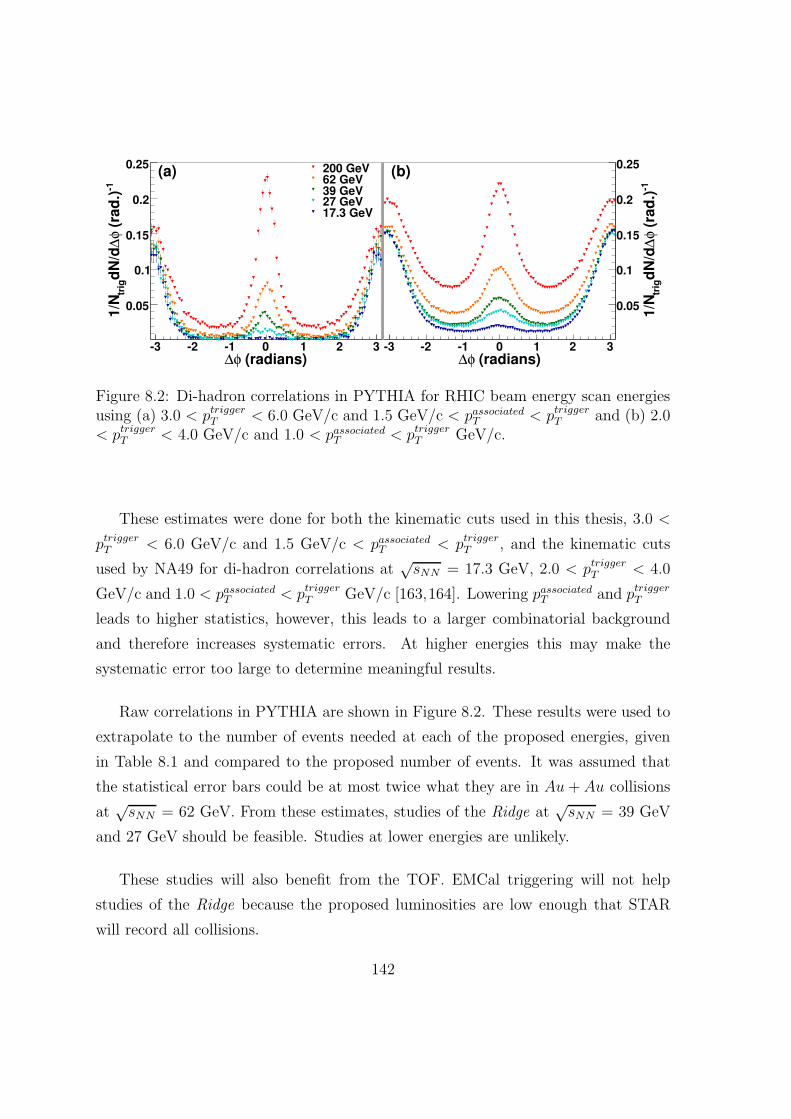
(radians)φ∆-3 -2 -1 0 1 2 3

-1 (

rad

.)φ

∆d

N/d

trig

1/N 0.05

0.1

0.15

0.2

0.25 200 GeV62 GeV39 GeV27 GeV17.3 GeV

(a)

(radians)φ∆-3 -2 -1 0 1 2 3

-1 (

rad

.)φ

∆d

N/d

trig

1/N0.05

0.1

0.15

0.2

0.25(b)

Figure 8.2: Di-hadron correlations in PYTHIA for RHIC beam energy scan energiesusing (a) 3.0 < ptrigger

T < 6.0 GeV/c and 1.5 GeV/c < passociatedT < ptrigger

T and (b) 2.0< ptrigger

T < 4.0 GeV/c and 1.0 < passociatedT < ptrigger

T GeV/c.

These estimates were done for both the kinematic cuts used in this thesis, 3.0 <

ptriggerT < 6.0 GeV/c and 1.5 GeV/c < passociated

T < ptriggerT , and the kinematic cuts

used by NA49 for di-hadron correlations at√sNN = 17.3 GeV, 2.0 < ptrigger

T < 4.0

GeV/c and 1.0 < passociatedT < ptrigger

T GeV/c [163,164]. Lowering passociatedT and ptrigger

T

leads to higher statistics, however, this leads to a larger combinatorial background

and therefore increases systematic errors. At higher energies this may make the

systematic error too large to determine meaningful results.

Raw correlations in PYTHIA are shown in Figure 8.2. These results were used to

extrapolate to the number of events needed at each of the proposed energies, given

in Table 8.1 and compared to the proposed number of events. It was assumed that

the statistical error bars could be at most twice what they are in Au+ Au collisions

at√sNN = 62 GeV. From these estimates, studies of the Ridge at

√sNN = 39 GeV

and 27 GeV should be feasible. Studies at lower energies are unlikely.

These studies will also benefit from the TOF. EMCal triggering will not help

studies of the Ridge because the proposed luminosities are low enough that STAR

will record all collisions.

142

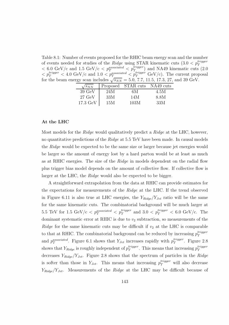
Table 8.1: Number of events proposed for the RHIC beam energy scan and the numberof events needed for studies of the Ridge using STAR kinematic cuts (3.0 < ptrigger

T

< 6.0 GeV/c and 1.5 GeV/c < passociatedT < ptrigger

T ) and NA49 kinematic cuts (2.0< ptrigger

T < 4.0 GeV/c and 1.0 < passociatedT < ptrigger

T GeV/c). The current proposalfor the beam energy scan includes

√sNN = 5.0, 7.7, 11.5, 17.3, 27, and 39 GeV.√

sNN Proposed STAR cuts NA49 cuts39 GeV 24M 6M 4.5M27 GeV 33M 14M 8.8M

17.3 GeV 15M 103M 33M

At the LHC

Most models for the Ridge would qualitatively predict a Ridge at the LHC, however,

no quantitative predictions of the Ridge at 5.5 TeV have been made. In causal models

the Ridge would be expected to be the same size or larger because jet energies would

be larger so the amount of energy lost by a hard parton would be at least as much

as at RHIC energies. The size of the Ridge in models dependent on the radial flow

plus trigger bias model depends on the amount of collective flow. If collective flow is

larger at the LHC, the Ridge would also be expected to be bigger.

A straightforward extrapolation from the data at RHIC can provide estimates for

the expectations for measurements of the Ridge at the LHC. If the trend observed

in Figure 6.11 is also true at LHC energies, the YRidge/YJet ratio will be the same

for the same kinematic cuts. The combinatorial background will be much larger at

5.5 TeV for 1.5 GeV/c < passociatedT < ptrigger

T and 3.0 < ptriggerT < 6.0 GeV/c. The

dominant systematic error at RHIC is due to v2 subtraction, so measurements of the

Ridge for the same kinematic cuts may be difficult if v2 at the LHC is comparable

to that at RHIC. The combinatorial background can be reduced by increasing ptriggerT

and passociatedT . Figure 6.1 shows that YJet increases rapidly with ptrigger

T . Figure 2.8

shows that YRidge is roughly independent of ptriggerT . This means that increasing ptrigger

T

decreases YRidge/YJet. Figure 2.8 shows that the spectrum of particles in the Ridge

is softer than those in YJet. This means that increasing ptriggerT will also decrease

YRidge/YJet. Measurements of the Ridge at the LHC may be difficult because of

143

the large combinatorial background if these naive extrapolations of RHIC data are

correct.

144

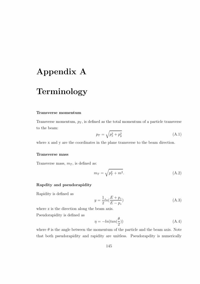
Appendix A

Terminology

Transverse momentum

Transverse momentum, pT , is defined as the total momentum of a particle transverse

to the beam:

pT =√

p2x + p2

y (A.1)

where x and y are the coordinates in the plane transverse to the beam direction.

Transverse mass

Transverse mass, mT , is defined as:

mT =√

p2T +m2. (A.2)

Rapdity and pseudorapidity

Rapidity is defined as

y =1

2ln(

E + pz

E − pz) (A.3)

where z is the direction along the beam axis.

Pseudorapidity is defined as

η = −ln(tan(θ

2)) (A.4)

where θ is the angle between the momentum of the particle and the beam axis. Note

that both pseudorapidity and rapidity are unitless. Pseudorapdity is numerically

145

Figure A.1: Rapidity and pseudorapidity for different particle species

close to rapidity for light particles at midrapidity traveling near the speed of light.

Figure A.1 shows the rapidity and pseudorapidity for particles with pT = 1 GeV/c

for particles with different masses. At y = 0, η = y. For a pion, y and η are almost

the same, however, the difference is large for a heavy particle such as a D meson.

146

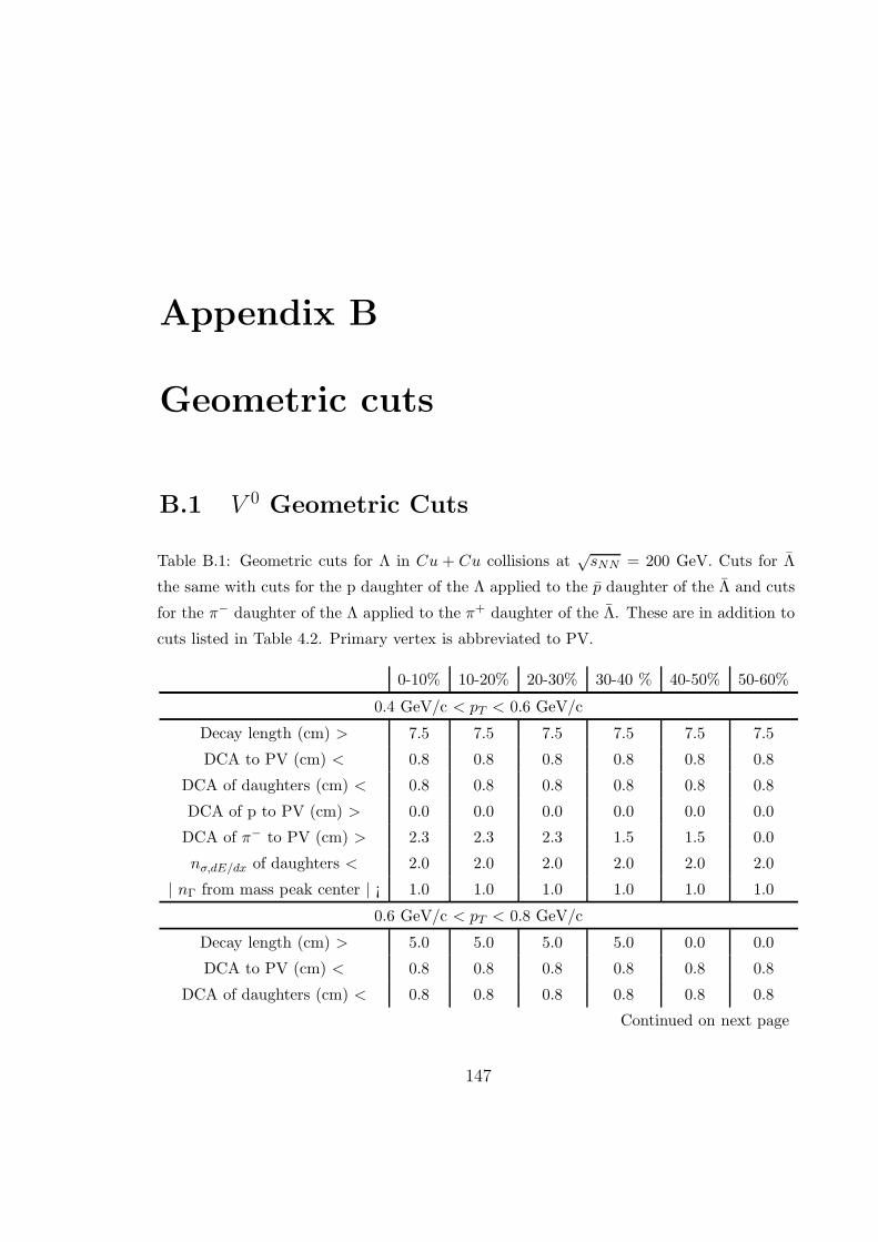
Appendix B

Geometric cuts

B.1 V 0 Geometric Cuts

Table B.1: Geometric cuts for Λ in Cu + Cu collisions at√

sNN = 200 GeV. Cuts for Λ

the same with cuts for the p daughter of the Λ applied to the p daughter of the Λ and cuts

for the π− daughter of the Λ applied to the π+ daughter of the Λ. These are in addition to

cuts listed in Table 4.2. Primary vertex is abbreviated to PV.

0-10% 10-20% 20-30% 30-40 % 40-50% 50-60%

0.4 GeV/c < pT < 0.6 GeV/c

Decay length (cm) > 7.5 7.5 7.5 7.5 7.5 7.5

DCA to PV (cm) < 0.8 0.8 0.8 0.8 0.8 0.8

DCA of daughters (cm) < 0.8 0.8 0.8 0.8 0.8 0.8

DCA of p to PV (cm) > 0.0 0.0 0.0 0.0 0.0 0.0

DCA of π− to PV (cm) > 2.3 2.3 2.3 1.5 1.5 0.0

nσ,dE/dx of daughters < 2.0 2.0 2.0 2.0 2.0 2.0

| nΓ from mass peak center | ¡ 1.0 1.0 1.0 1.0 1.0 1.0

0.6 GeV/c < pT < 0.8 GeV/c

Decay length (cm) > 5.0 5.0 5.0 5.0 0.0 0.0

DCA to PV (cm) < 0.8 0.8 0.8 0.8 0.8 0.8

DCA of daughters (cm) < 0.8 0.8 0.8 0.8 0.8 0.8

Continued on next page

147

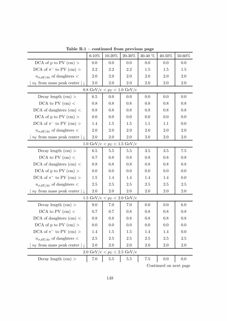
Table B.1 – continued from previous page

0-10% 10-20% 20-30% 30-40 % 40-50% 50-60%

DCA of p to PV (cm) > 0.0 0.0 0.0 0.0 0.0 0.0

DCA of π− to PV (cm) > 2.2 2.2 2.2 1.5 1.5 1.5

nσ,dE/dx of daughters < 2.0 2.0 2.0 2.0 2.0 2.0

| nΓ from mass peak center | ¡ 2.0 2.0 2.0 2.0 2.0 2.0

0.8 GeV/c < pT < 1.0 GeV/c

Decay length (cm) > 6.5 0.0 0.0 0.0 0.0 0.0

DCA to PV (cm) < 0.8 0.8 0.8 0.8 0.8 0.8

DCA of daughters (cm) < 0.8 0.8 0.8 0.8 0.8 0.8

DCA of p to PV (cm) > 0.0 0.0 0.0 0.0 0.0 0.0

DCA of π− to PV (cm) > 1.4 1.5 1.5 1.1 1.1 0.0

nσ,dE/dx of daughters < 2.0 2.0 2.0 2.0 2.0 2.0

| nΓ from mass peak center | ¡ 2.0 2.0 2.0 2.0 2.0 2.0

1.0 GeV/c < pT < 1.5 GeV/c

Decay length (cm) > 6.5 5.5 5.5 3.5 3.5 7.5

DCA to PV (cm) < 0.7 0.8 0.8 0.8 0.8 0.8

DCA of daughters (cm) < 0.8 0.8 0.8 0.8 0.8 0.8

DCA of p to PV (cm) > 0.0 0.0 0.0 0.0 0.0 0.0

DCA of π− to PV (cm) > 1.5 1.4 1.4 1.4 1.4 0.0

nσ,dE/dx of daughters < 2.5 2.5 2.5 2.5 2.5 2.5

| nΓ from mass peak center | ¡ 2.0 2.0 2.0 2.0 2.0 2.0

1.5 GeV/c < pT < 2.0 GeV/c

Decay length (cm) > 9.0 7.0 7.0 0.0 0.0 6.0

DCA to PV (cm) < 0.7 0.7 0.8 0.8 0.8 0.8

DCA of daughters (cm) < 0.8 0.8 0.8 0.8 0.8 0.8

DCA of p to PV (cm) > 0.0 0.0 0.0 0.0 0.0 0.0

DCA of π− to PV (cm) > 1.4 1.5 1.5 1.4 1.4 0.0

nσ,dE/dx of daughters < 2.5 2.5 2.5 2.5 2.5 2.5

| nΓ from mass peak center | ¡ 2.0 2.0 2.0 2.0 2.0 2.0

2.0 GeV/c < pT < 2.5 GeV/c

Decay length (cm) > 7.0 5.5 5.5 7.5 0.0 0.0

Continued on next page

148

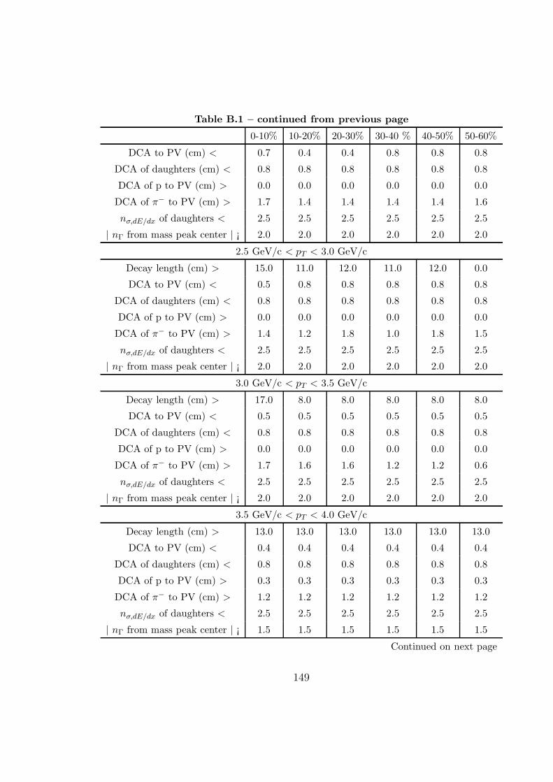
Table B.1 – continued from previous page

0-10% 10-20% 20-30% 30-40 % 40-50% 50-60%

DCA to PV (cm) < 0.7 0.4 0.4 0.8 0.8 0.8

DCA of daughters (cm) < 0.8 0.8 0.8 0.8 0.8 0.8

DCA of p to PV (cm) > 0.0 0.0 0.0 0.0 0.0 0.0

DCA of π− to PV (cm) > 1.7 1.4 1.4 1.4 1.4 1.6

nσ,dE/dx of daughters < 2.5 2.5 2.5 2.5 2.5 2.5

| nΓ from mass peak center | ¡ 2.0 2.0 2.0 2.0 2.0 2.0

2.5 GeV/c < pT < 3.0 GeV/c

Decay length (cm) > 15.0 11.0 12.0 11.0 12.0 0.0

DCA to PV (cm) < 0.5 0.8 0.8 0.8 0.8 0.8

DCA of daughters (cm) < 0.8 0.8 0.8 0.8 0.8 0.8

DCA of p to PV (cm) > 0.0 0.0 0.0 0.0 0.0 0.0

DCA of π− to PV (cm) > 1.4 1.2 1.8 1.0 1.8 1.5

nσ,dE/dx of daughters < 2.5 2.5 2.5 2.5 2.5 2.5

| nΓ from mass peak center | ¡ 2.0 2.0 2.0 2.0 2.0 2.0

3.0 GeV/c < pT < 3.5 GeV/c

Decay length (cm) > 17.0 8.0 8.0 8.0 8.0 8.0

DCA to PV (cm) < 0.5 0.5 0.5 0.5 0.5 0.5

DCA of daughters (cm) < 0.8 0.8 0.8 0.8 0.8 0.8

DCA of p to PV (cm) > 0.0 0.0 0.0 0.0 0.0 0.0

DCA of π− to PV (cm) > 1.7 1.6 1.6 1.2 1.2 0.6

nσ,dE/dx of daughters < 2.5 2.5 2.5 2.5 2.5 2.5

| nΓ from mass peak center | ¡ 2.0 2.0 2.0 2.0 2.0 2.0

3.5 GeV/c < pT < 4.0 GeV/c

Decay length (cm) > 13.0 13.0 13.0 13.0 13.0 13.0

DCA to PV (cm) < 0.4 0.4 0.4 0.4 0.4 0.4

DCA of daughters (cm) < 0.8 0.8 0.8 0.8 0.8 0.8

DCA of p to PV (cm) > 0.3 0.3 0.3 0.3 0.3 0.3

DCA of π− to PV (cm) > 1.2 1.2 1.2 1.2 1.2 1.2

nσ,dE/dx of daughters < 2.5 2.5 2.5 2.5 2.5 2.5

| nΓ from mass peak center | ¡ 1.5 1.5 1.5 1.5 1.5 1.5

Continued on next page

149

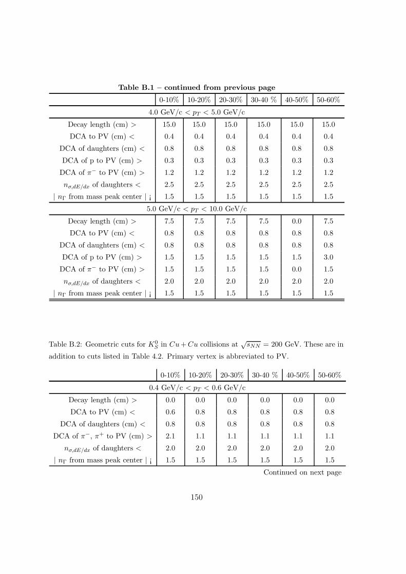
Table B.1 – continued from previous page

0-10% 10-20% 20-30% 30-40 % 40-50% 50-60%

4.0 GeV/c < pT < 5.0 GeV/c

Decay length (cm) > 15.0 15.0 15.0 15.0 15.0 15.0

DCA to PV (cm) < 0.4 0.4 0.4 0.4 0.4 0.4

DCA of daughters (cm) < 0.8 0.8 0.8 0.8 0.8 0.8

DCA of p to PV (cm) > 0.3 0.3 0.3 0.3 0.3 0.3

DCA of π− to PV (cm) > 1.2 1.2 1.2 1.2 1.2 1.2

nσ,dE/dx of daughters < 2.5 2.5 2.5 2.5 2.5 2.5

| nΓ from mass peak center | ¡ 1.5 1.5 1.5 1.5 1.5 1.5

5.0 GeV/c < pT < 10.0 GeV/c

Decay length (cm) > 7.5 7.5 7.5 7.5 0.0 7.5

DCA to PV (cm) < 0.8 0.8 0.8 0.8 0.8 0.8

DCA of daughters (cm) < 0.8 0.8 0.8 0.8 0.8 0.8

DCA of p to PV (cm) > 1.5 1.5 1.5 1.5 1.5 3.0

DCA of π− to PV (cm) > 1.5 1.5 1.5 1.5 0.0 1.5

nσ,dE/dx of daughters < 2.0 2.0 2.0 2.0 2.0 2.0

| nΓ from mass peak center | ¡ 1.5 1.5 1.5 1.5 1.5 1.5

Table B.2: Geometric cuts for K0S in Cu+ Cu collisions at

√sNN = 200 GeV. These are in

addition to cuts listed in Table 4.2. Primary vertex is abbreviated to PV.

0-10% 10-20% 20-30% 30-40 % 40-50% 50-60%

0.4 GeV/c < pT < 0.6 GeV/c

Decay length (cm) > 0.0 0.0 0.0 0.0 0.0 0.0

DCA to PV (cm) < 0.6 0.8 0.8 0.8 0.8 0.8

DCA of daughters (cm) < 0.8 0.8 0.8 0.8 0.8 0.8

DCA of π−, π+ to PV (cm) > 2.1 1.1 1.1 1.1 1.1 1.1

nσ,dE/dx of daughters < 2.0 2.0 2.0 2.0 2.0 2.0

| nΓ from mass peak center | ¡ 1.5 1.5 1.5 1.5 1.5 1.5

Continued on next page

150

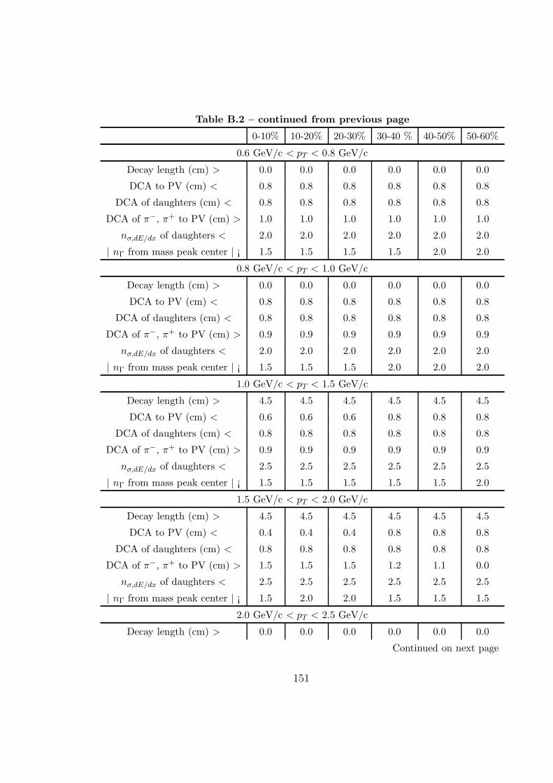
Table B.2 – continued from previous page

0-10% 10-20% 20-30% 30-40 % 40-50% 50-60%

0.6 GeV/c < pT < 0.8 GeV/c

Decay length (cm) > 0.0 0.0 0.0 0.0 0.0 0.0

DCA to PV (cm) < 0.8 0.8 0.8 0.8 0.8 0.8

DCA of daughters (cm) < 0.8 0.8 0.8 0.8 0.8 0.8

DCA of π−, π+ to PV (cm) > 1.0 1.0 1.0 1.0 1.0 1.0

nσ,dE/dx of daughters < 2.0 2.0 2.0 2.0 2.0 2.0

| nΓ from mass peak center | ¡ 1.5 1.5 1.5 1.5 2.0 2.0

0.8 GeV/c < pT < 1.0 GeV/c

Decay length (cm) > 0.0 0.0 0.0 0.0 0.0 0.0

DCA to PV (cm) < 0.8 0.8 0.8 0.8 0.8 0.8

DCA of daughters (cm) < 0.8 0.8 0.8 0.8 0.8 0.8

DCA of π−, π+ to PV (cm) > 0.9 0.9 0.9 0.9 0.9 0.9

nσ,dE/dx of daughters < 2.0 2.0 2.0 2.0 2.0 2.0

| nΓ from mass peak center | ¡ 1.5 1.5 1.5 2.0 2.0 2.0

1.0 GeV/c < pT < 1.5 GeV/c

Decay length (cm) > 4.5 4.5 4.5 4.5 4.5 4.5

DCA to PV (cm) < 0.6 0.6 0.6 0.8 0.8 0.8

DCA of daughters (cm) < 0.8 0.8 0.8 0.8 0.8 0.8

DCA of π−, π+ to PV (cm) > 0.9 0.9 0.9 0.9 0.9 0.9

nσ,dE/dx of daughters < 2.5 2.5 2.5 2.5 2.5 2.5

| nΓ from mass peak center | ¡ 1.5 1.5 1.5 1.5 1.5 2.0

1.5 GeV/c < pT < 2.0 GeV/c

Decay length (cm) > 4.5 4.5 4.5 4.5 4.5 4.5

DCA to PV (cm) < 0.4 0.4 0.4 0.8 0.8 0.8

DCA of daughters (cm) < 0.8 0.8 0.8 0.8 0.8 0.8

DCA of π−, π+ to PV (cm) > 1.5 1.5 1.5 1.2 1.1 0.0

nσ,dE/dx of daughters < 2.5 2.5 2.5 2.5 2.5 2.5

| nΓ from mass peak center | ¡ 1.5 2.0 2.0 1.5 1.5 1.5

2.0 GeV/c < pT < 2.5 GeV/c

Decay length (cm) > 0.0 0.0 0.0 0.0 0.0 0.0

Continued on next page

151

Table B.2 – continued from previous page

0-10% 10-20% 20-30% 30-40 % 40-50% 50-60%

DCA to PV (cm) < 0.4 0.4 0.4 0.8 0.8 0.8

DCA of daughters (cm) < 0.8 0.8 0.8 0.8 0.8 0.8

DCA of π−, π+ to PV (cm) > 1.6 1.4 1.4 1.4 1.1 1.1

nσ,dE/dx of daughters < 2.5 2.5 2.5 2.5 2.5 2.5

| nΓ from mass peak center | ¡ 1.5 2.0 2.0 1.5 1.5 1.5

2.5 GeV/c < pT < 3.0 GeV/c

Decay length (cm) > 0.0 0.0 0.0 0.0 0.0 0.0

DCA to PV (cm) < 0.4 0.4 0.4 0.4 0.4 0.4

DCA of daughters (cm) < 0.8 0.8 0.8 0.8 0.8 0.8

DCA of π−, π+ to PV (cm) > 1.2 1.2 1.0 0.0 0.0 0.0

nσ,dE/dx of daughters < 2.5 2.5 2.5 2.5 2.5 2.5

| nΓ from mass peak center | ¡ 1.5 2.0 2.0 1.5 2.0 2.0

3.0 GeV/c < pT < 3.5 GeV/c

Decay length (cm) > 0.0 0.0 0.0 0.0 0.0 0.0

DCA to PV (cm) < 0.4 0.4 0.4 0.5 0.5 0.5

DCA of daughters (cm) < 0.8 0.8 0.8 0.8 0.8 0.8

DCA of π−, π+ to PV (cm) > 0.8 0.8 0.8 0.8 0.8 0.8

nσ,dE/dx of daughters < 2.5 2.5 2.5 2.5 2.5 2.5

| nΓ from mass peak center | ¡ 1.5 1.5 1.5 1.5 1.5 2.0

3.5 GeV/c < pT < 4.0 GeV/c

Decay length (cm) > 0.0 0.0 0.0 0.0 0.0 0.0

DCA to PV (cm) < 0.4 0.4 0.4 0.4 0.4 0.4

DCA of daughters (cm) < 0.8 0.8 0.8 0.8 0.8 0.8

DCA of π−, π+ to PV (cm) > 0.8 0.8 0.6 0.6 0.6 0.6

nσ,dE/dx of daughters < 2.5 2.5 2.5 2.5 2.5 2.5

| nΓ from mass peak center | ¡ 1.5 1.5 1.5 1.5 1.5 1.5

4.0 GeV/c < pT < 5.0 GeV/c

Decay length (cm) > 0.0 0.0 0.0 0.0 0.0 0.0

DCA to PV (cm) < 0.4 0.4 0.4 0.4 0.4 0.4

DCA of daughters (cm) < 0.8 0.8 0.8 0.8 0.8 0.8

Continued on next page

152

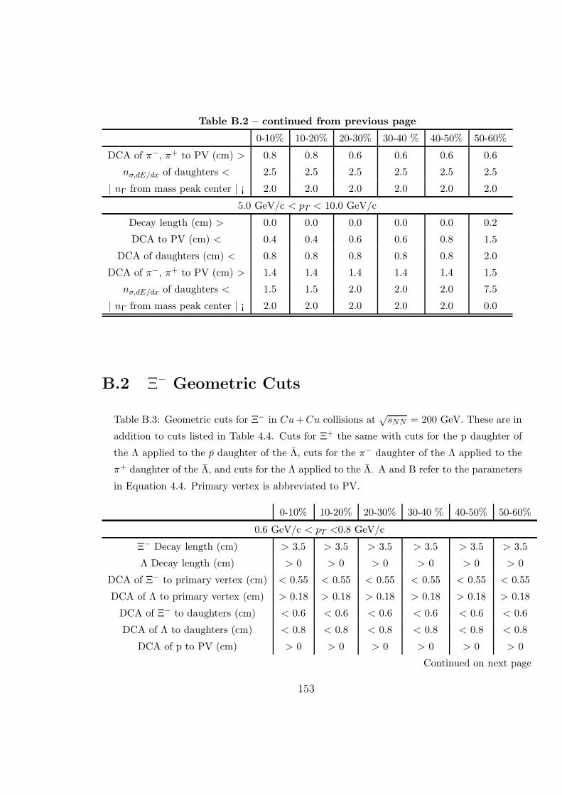
Table B.2 – continued from previous page

0-10% 10-20% 20-30% 30-40 % 40-50% 50-60%

DCA of π−, π+ to PV (cm) > 0.8 0.8 0.6 0.6 0.6 0.6

nσ,dE/dx of daughters < 2.5 2.5 2.5 2.5 2.5 2.5

| nΓ from mass peak center | ¡ 2.0 2.0 2.0 2.0 2.0 2.0

5.0 GeV/c < pT < 10.0 GeV/c

Decay length (cm) > 0.0 0.0 0.0 0.0 0.0 0.2

DCA to PV (cm) < 0.4 0.4 0.6 0.6 0.8 1.5

DCA of daughters (cm) < 0.8 0.8 0.8 0.8 0.8 2.0

DCA of π−, π+ to PV (cm) > 1.4 1.4 1.4 1.4 1.4 1.5

nσ,dE/dx of daughters < 1.5 1.5 2.0 2.0 2.0 7.5

| nΓ from mass peak center | ¡ 2.0 2.0 2.0 2.0 2.0 0.0

B.2 Ξ− Geometric Cuts

Table B.3: Geometric cuts for Ξ− in Cu + Cu collisions at√

sNN = 200 GeV. These are in

addition to cuts listed in Table 4.4. Cuts for Ξ+ the same with cuts for the p daughter of

the Λ applied to the p daughter of the Λ, cuts for the π− daughter of the Λ applied to the

π+ daughter of the Λ, and cuts for the Λ applied to the Λ. A and B refer to the parameters

in Equation 4.4. Primary vertex is abbreviated to PV.

0-10% 10-20% 20-30% 30-40 % 40-50% 50-60%

0.6 GeV/c < pT <0.8 GeV/c

Ξ− Decay length (cm) > 3.5 > 3.5 > 3.5 > 3.5 > 3.5 > 3.5

Λ Decay length (cm) > 0 > 0 > 0 > 0 > 0 > 0

DCA of Ξ− to primary vertex (cm) < 0.55 < 0.55 < 0.55 < 0.55 < 0.55 < 0.55

DCA of Λ to primary vertex (cm) > 0.18 > 0.18 > 0.18 > 0.18 > 0.18 > 0.18

DCA of Ξ− to daughters (cm) < 0.6 < 0.6 < 0.6 < 0.6 < 0.6 < 0.6

DCA of Λ to daughters (cm) < 0.8 < 0.8 < 0.8 < 0.8 < 0.8 < 0.8

DCA of p to PV (cm) > 0 > 0 > 0 > 0 > 0 > 0

Continued on next page

153

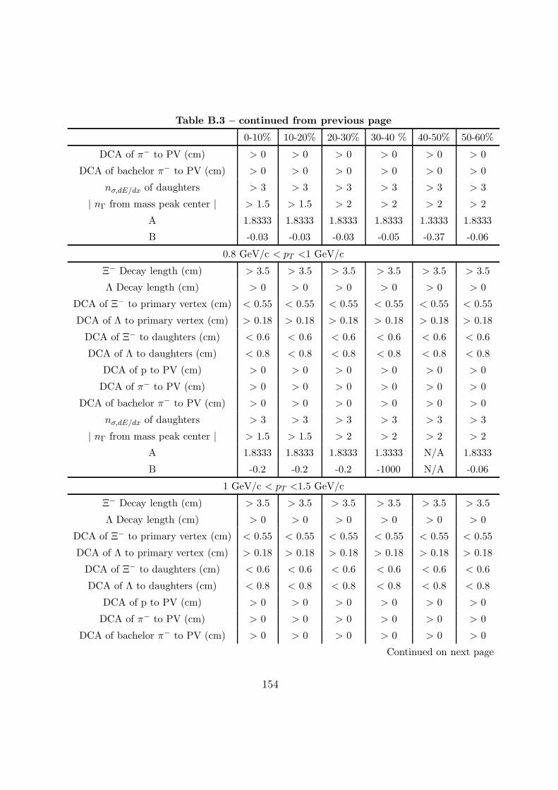
Table B.3 – continued from previous page

0-10% 10-20% 20-30% 30-40 % 40-50% 50-60%

DCA of π− to PV (cm) > 0 > 0 > 0 > 0 > 0 > 0

DCA of bachelor π− to PV (cm) > 0 > 0 > 0 > 0 > 0 > 0

nσ,dE/dx of daughters > 3 > 3 > 3 > 3 > 3 > 3

| nΓ from mass peak center | > 1.5 > 1.5 > 2 > 2 > 2 > 2

A 1.8333 1.8333 1.8333 1.8333 1.3333 1.8333

B -0.03 -0.03 -0.03 -0.05 -0.37 -0.06

0.8 GeV/c < pT <1 GeV/c

Ξ− Decay length (cm) > 3.5 > 3.5 > 3.5 > 3.5 > 3.5 > 3.5

Λ Decay length (cm) > 0 > 0 > 0 > 0 > 0 > 0

DCA of Ξ− to primary vertex (cm) < 0.55 < 0.55 < 0.55 < 0.55 < 0.55 < 0.55

DCA of Λ to primary vertex (cm) > 0.18 > 0.18 > 0.18 > 0.18 > 0.18 > 0.18

DCA of Ξ− to daughters (cm) < 0.6 < 0.6 < 0.6 < 0.6 < 0.6 < 0.6

DCA of Λ to daughters (cm) < 0.8 < 0.8 < 0.8 < 0.8 < 0.8 < 0.8

DCA of p to PV (cm) > 0 > 0 > 0 > 0 > 0 > 0

DCA of π− to PV (cm) > 0 > 0 > 0 > 0 > 0 > 0

DCA of bachelor π− to PV (cm) > 0 > 0 > 0 > 0 > 0 > 0

nσ,dE/dx of daughters > 3 > 3 > 3 > 3 > 3 > 3

| nΓ from mass peak center | > 1.5 > 1.5 > 2 > 2 > 2 > 2

A 1.8333 1.8333 1.8333 1.3333 N/A 1.8333

B -0.2 -0.2 -0.2 -1000 N/A -0.06

1 GeV/c < pT <1.5 GeV/c

Ξ− Decay length (cm) > 3.5 > 3.5 > 3.5 > 3.5 > 3.5 > 3.5

Λ Decay length (cm) > 0 > 0 > 0 > 0 > 0 > 0

DCA of Ξ− to primary vertex (cm) < 0.55 < 0.55 < 0.55 < 0.55 < 0.55 < 0.55

DCA of Λ to primary vertex (cm) > 0.18 > 0.18 > 0.18 > 0.18 > 0.18 > 0.18

DCA of Ξ− to daughters (cm) < 0.6 < 0.6 < 0.6 < 0.6 < 0.6 < 0.6

DCA of Λ to daughters (cm) < 0.8 < 0.8 < 0.8 < 0.8 < 0.8 < 0.8

DCA of p to PV (cm) > 0 > 0 > 0 > 0 > 0 > 0

DCA of π− to PV (cm) > 0 > 0 > 0 > 0 > 0 > 0

DCA of bachelor π− to PV (cm) > 0 > 0 > 0 > 0 > 0 > 0

Continued on next page

154

Table B.3 – continued from previous page

0-10% 10-20% 20-30% 30-40 % 40-50% 50-60%

nσ,dE/dx of daughters > 3 > 3 > 3 > 3 > 3 > 3

| nΓ from mass peak center | > 1.5 > 1.5 > 2 > 2 > 2 > 2

A 1.3333 1.3333 1.3333 N/A N/A 1.8333

B -0.35 -0.35 -0.35 N/A N/A -0.06

1.5 GeV/c < pT <2 GeV/c

Ξ− Decay length (cm) > 3.5 > 3.5 > 3.5 > 3.5 > 3.5 > 3.5

Λ Decay length (cm) > 0 > 0 > 0 > 0 > 0 > 0

DCA of Ξ− to primary vertex (cm) < 0.55 < 0.55 < 0.55 < 0.55 < 0.55 < 0.55

DCA of Λ to primary vertex (cm) > 0.18 > 0.18 > 0.18 > 0.18 > 0.18 > 0.18

DCA of Ξ− to daughters (cm) < 0.6 < 0.6 < 0.6 < 0.6 < 0.6 < 0.6

DCA of Λ to daughters (cm) < 0.8 < 0.8 < 0.8 < 0.8 < 0.8 < 0.8

DCA of p to PV (cm) > 0 > 0 > 0 > 0 > 0 > 0

DCA of π− to PV (cm) > 0 > 0 > 0 > 0 > 0 > 0

DCA of bachelor π− to PV (cm) > 0 > 0 > 0 > 0 > 0 > 0

nσ,dE/dx of daughters > 3 > 3 > 3 > 3 > 3 > 3

| nΓ from mass peak center | > 1.5 > 1.5 > 2 > 2 > 2 > 2

A 1.3333 1.3333 1.3333 N/A N/A 1.8333

B -0.4 -0.4 -0.4 N/A N/A -0.06

2 GeV/c < pT <2.5 GeV/c

Ξ− Decay length (cm) > 3.5 > 3.5 > 3.5 > 3.5 > 3.5 > 3.5

Λ Decay length (cm) > 0 > 0 > 0 > 0 > 0 > 0

DCA of Ξ− to primary vertex (cm) < 0.55 < 0.55 < 0.55 < 0.55 < 0.55 < 0.55

DCA of Λ to primary vertex (cm) > 0.18 > 0.18 > 0.18 > 0.18 > 0.18 > 0.18

DCA of Ξ− to daughters (cm) < 0.6 < 0.6 < 0.6 < 0.6 < 0.6 < 0.6

DCA of Λ to daughters (cm) < 0.8 < 0.8 < 0.8 < 0.8 < 0.8 < 0.8

DCA of p to PV (cm) > 0 > 0 > 0 > 0 > 0 > 0

DCA of π− to PV (cm) > 0 > 0 > 0 > 0 > 0 > 0

DCA of bachelor π− to PV (cm) > 0 > 0 > 0 > 0 > 0 > 0

nσ,dE/dx of daughters > 3 > 3 > 3 > 3 > 3 > 3

| nΓ from mass peak center | > 1.5 > 1.5 > 2 > 2 > 2 > 2

Continued on next page

155

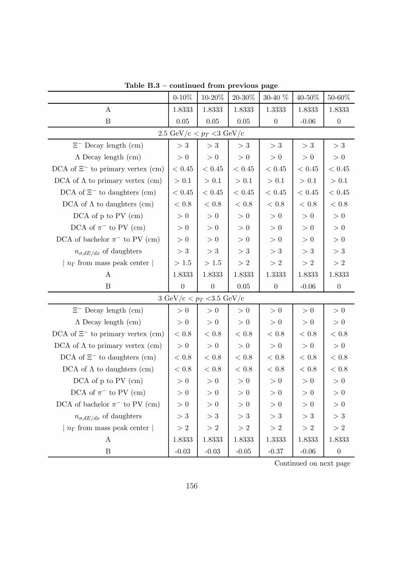
Table B.3 – continued from previous page

0-10% 10-20% 20-30% 30-40 % 40-50% 50-60%

A 1.8333 1.8333 1.8333 1.3333 1.8333 1.8333

B 0.05 0.05 0.05 0 -0.06 0

2.5 GeV/c < pT <3 GeV/c

Ξ− Decay length (cm) > 3 > 3 > 3 > 3 > 3 > 3

Λ Decay length (cm) > 0 > 0 > 0 > 0 > 0 > 0

DCA of Ξ− to primary vertex (cm) < 0.45 < 0.45 < 0.45 < 0.45 < 0.45 < 0.45

DCA of Λ to primary vertex (cm) > 0.1 > 0.1 > 0.1 > 0.1 > 0.1 > 0.1

DCA of Ξ− to daughters (cm) < 0.45 < 0.45 < 0.45 < 0.45 < 0.45 < 0.45

DCA of Λ to daughters (cm) < 0.8 < 0.8 < 0.8 < 0.8 < 0.8 < 0.8

DCA of p to PV (cm) > 0 > 0 > 0 > 0 > 0 > 0

DCA of π− to PV (cm) > 0 > 0 > 0 > 0 > 0 > 0

DCA of bachelor π− to PV (cm) > 0 > 0 > 0 > 0 > 0 > 0

nσ,dE/dx of daughters > 3 > 3 > 3 > 3 > 3 > 3

| nΓ from mass peak center | > 1.5 > 1.5 > 2 > 2 > 2 > 2

A 1.8333 1.8333 1.8333 1.3333 1.8333 1.8333

B 0 0 0.05 0 -0.06 0

3 GeV/c < pT <3.5 GeV/c

Ξ− Decay length (cm) > 0 > 0 > 0 > 0 > 0 > 0

Λ Decay length (cm) > 0 > 0 > 0 > 0 > 0 > 0

DCA of Ξ− to primary vertex (cm) < 0.8 < 0.8 < 0.8 < 0.8 < 0.8 < 0.8

DCA of Λ to primary vertex (cm) > 0 > 0 > 0 > 0 > 0 > 0

DCA of Ξ− to daughters (cm) < 0.8 < 0.8 < 0.8 < 0.8 < 0.8 < 0.8

DCA of Λ to daughters (cm) < 0.8 < 0.8 < 0.8 < 0.8 < 0.8 < 0.8

DCA of p to PV (cm) > 0 > 0 > 0 > 0 > 0 > 0

DCA of π− to PV (cm) > 0 > 0 > 0 > 0 > 0 > 0

DCA of bachelor π− to PV (cm) > 0 > 0 > 0 > 0 > 0 > 0

nσ,dE/dx of daughters > 3 > 3 > 3 > 3 > 3 > 3

| nΓ from mass peak center | > 2 > 2 > 2 > 2 > 2 > 2

A 1.8333 1.8333 1.8333 1.3333 1.8333 1.8333

B -0.03 -0.03 -0.05 -0.37 -0.06 0

Continued on next page

156

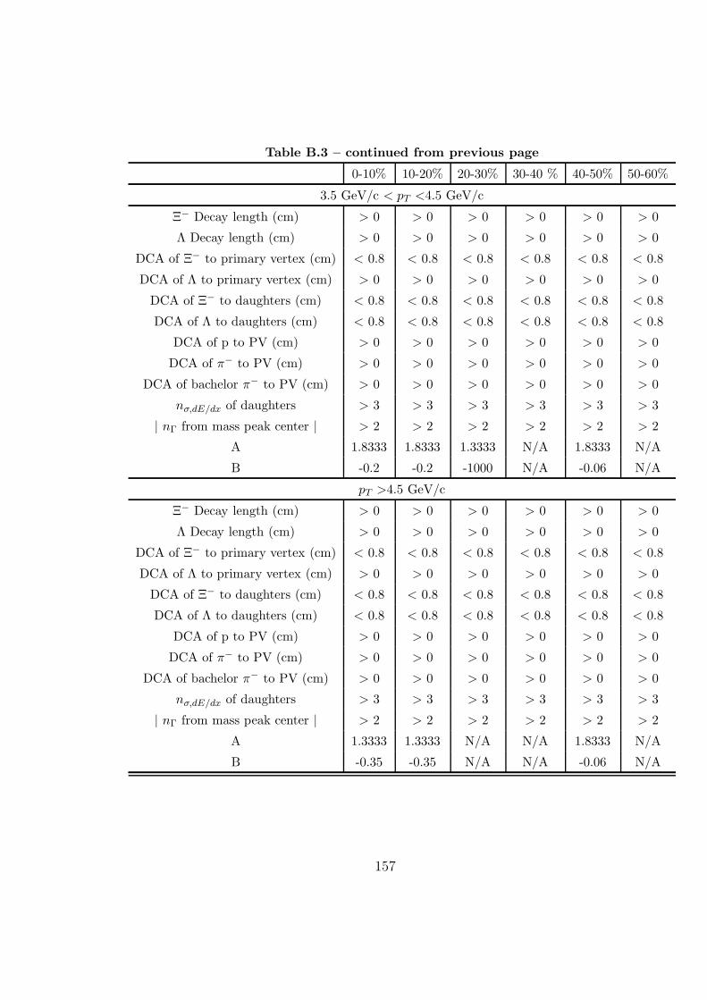
Table B.3 – continued from previous page

0-10% 10-20% 20-30% 30-40 % 40-50% 50-60%

3.5 GeV/c < pT <4.5 GeV/c

Ξ− Decay length (cm) > 0 > 0 > 0 > 0 > 0 > 0

Λ Decay length (cm) > 0 > 0 > 0 > 0 > 0 > 0

DCA of Ξ− to primary vertex (cm) < 0.8 < 0.8 < 0.8 < 0.8 < 0.8 < 0.8

DCA of Λ to primary vertex (cm) > 0 > 0 > 0 > 0 > 0 > 0

DCA of Ξ− to daughters (cm) < 0.8 < 0.8 < 0.8 < 0.8 < 0.8 < 0.8

DCA of Λ to daughters (cm) < 0.8 < 0.8 < 0.8 < 0.8 < 0.8 < 0.8

DCA of p to PV (cm) > 0 > 0 > 0 > 0 > 0 > 0

DCA of π− to PV (cm) > 0 > 0 > 0 > 0 > 0 > 0

DCA of bachelor π− to PV (cm) > 0 > 0 > 0 > 0 > 0 > 0

nσ,dE/dx of daughters > 3 > 3 > 3 > 3 > 3 > 3

| nΓ from mass peak center | > 2 > 2 > 2 > 2 > 2 > 2

A 1.8333 1.8333 1.3333 N/A 1.8333 N/A

B -0.2 -0.2 -1000 N/A -0.06 N/A

pT >4.5 GeV/c

Ξ− Decay length (cm) > 0 > 0 > 0 > 0 > 0 > 0

Λ Decay length (cm) > 0 > 0 > 0 > 0 > 0 > 0

DCA of Ξ− to primary vertex (cm) < 0.8 < 0.8 < 0.8 < 0.8 < 0.8 < 0.8

DCA of Λ to primary vertex (cm) > 0 > 0 > 0 > 0 > 0 > 0

DCA of Ξ− to daughters (cm) < 0.8 < 0.8 < 0.8 < 0.8 < 0.8 < 0.8

DCA of Λ to daughters (cm) < 0.8 < 0.8 < 0.8 < 0.8 < 0.8 < 0.8

DCA of p to PV (cm) > 0 > 0 > 0 > 0 > 0 > 0

DCA of π− to PV (cm) > 0 > 0 > 0 > 0 > 0 > 0

DCA of bachelor π− to PV (cm) > 0 > 0 > 0 > 0 > 0 > 0

nσ,dE/dx of daughters > 3 > 3 > 3 > 3 > 3 > 3

| nΓ from mass peak center | > 2 > 2 > 2 > 2 > 2 > 2

A 1.3333 1.3333 N/A N/A 1.8333 N/A

B -0.35 -0.35 N/A N/A -0.06 N/A

157

158

Appendix C

Efficiencies

C.1 Unidentified hadron efficiencies

Table C.1: Fit parameters from fits of the efficiencies for unidentified hadrons inAu+ Au at

√sNN = 62 GeV to a exp( b

pT

c)

centrality a b c0-5% .767 .1498 1.3165-10% .7856 .1419 1.3310-20% .7975 .1408 1.46420-30% .8113 .1374 1.60630-40% .822 .1376 1.74340-50% .8321 .1327 1.78150-60% .8386 .1357 1.91260-70% .8387 .1511 2.38170-80% .8415 .1455 2.153

159

Table C.2: Fit parameters from fits of the efficiencies for unidentified hadrons inAu+ Au at

√sNN = 62 GeV to a exp( b

pT

c)

centrality a b c0-10% 0.838435 0.0704 0.940910-20% 0.843666 0.0681 1.000020-30% 0.843211 0.0610 1.000030-40% 0.848090 0.0638 1.000040-50% 0.856875 0.0606 0.949650-60% 0.851112 0.0584 1.0000

Table C.3: Fit parameters from fits of the efficiencies for unidentified hadrons inAu+ Au at

√sNN = 62 GeV to a exp( b

pT

c)

centrality a b c0-10% 0.8655 0.1333 0.989010-20% 0.8736 0.1207 0.933020-30% 0.8643 0.1503 1.107130-40% 0.8693 0.1269 0.992240-50% 0.8608 0.1511 1.161650-60% 0.8606 0.1971 1.3211

C.2 V 0 Efficiencies

Table C.4: Fit parameters from fits of the efficiencies for Λ baryons in Au + Au at√

sNN

= 62 GeV to a exp( bpT

c)

0-10% 10-20% 20-30% 30-40 % 40-50% 50-60%

1< pT <1.5

a 0.172 0.164 0.168 0.158 0.161 0.166

b 0.946 0.838 0.819 0.774 0.758 0.861

c 1.587 1.800 1.825 1.902 2.020 1.895

1.5< pT <2

a 0.174 0.162 0.169 0.159 0.161 0.164

b 1.043 0.887 0.855 0.772 0.755 0.821

Continued on next page

160

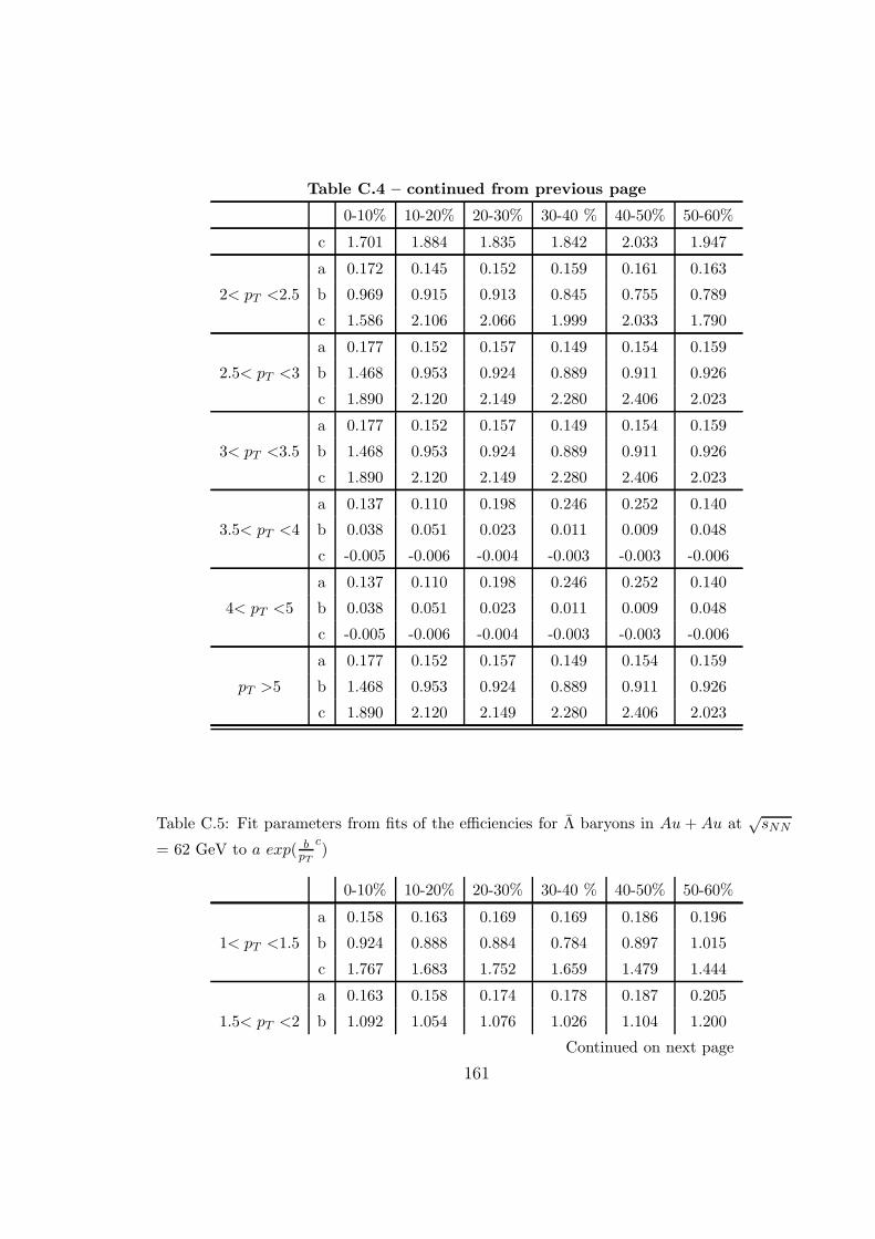
Table C.4 – continued from previous page

0-10% 10-20% 20-30% 30-40 % 40-50% 50-60%

c 1.701 1.884 1.835 1.842 2.033 1.947

2< pT <2.5

a 0.172 0.145 0.152 0.159 0.161 0.163

b 0.969 0.915 0.913 0.845 0.755 0.789

c 1.586 2.106 2.066 1.999 2.033 1.790

2.5< pT <3

a 0.177 0.152 0.157 0.149 0.154 0.159

b 1.468 0.953 0.924 0.889 0.911 0.926

c 1.890 2.120 2.149 2.280 2.406 2.023

3< pT <3.5

a 0.177 0.152 0.157 0.149 0.154 0.159

b 1.468 0.953 0.924 0.889 0.911 0.926

c 1.890 2.120 2.149 2.280 2.406 2.023

3.5< pT <4

a 0.137 0.110 0.198 0.246 0.252 0.140

b 0.038 0.051 0.023 0.011 0.009 0.048

c -0.005 -0.006 -0.004 -0.003 -0.003 -0.006

4< pT <5

a 0.137 0.110 0.198 0.246 0.252 0.140

b 0.038 0.051 0.023 0.011 0.009 0.048

c -0.005 -0.006 -0.004 -0.003 -0.003 -0.006

pT >5

a 0.177 0.152 0.157 0.149 0.154 0.159

b 1.468 0.953 0.924 0.889 0.911 0.926

c 1.890 2.120 2.149 2.280 2.406 2.023

Table C.5: Fit parameters from fits of the efficiencies for Λ baryons in Au + Au at√

sNN

= 62 GeV to a exp( bpT

c)

0-10% 10-20% 20-30% 30-40 % 40-50% 50-60%

1< pT <1.5

a 0.158 0.163 0.169 0.169 0.186 0.196

b 0.924 0.888 0.884 0.784 0.897 1.015

c 1.767 1.683 1.752 1.659 1.479 1.444

1.5< pT <2

a 0.163 0.158 0.174 0.178 0.187 0.205

b 1.092 1.054 1.076 1.026 1.104 1.200

Continued on next page

161

Table C.5 – continued from previous page

0-10% 10-20% 20-30% 30-40 % 40-50% 50-60%

c 1.948 2.156 1.950 1.763 1.758 1.527

2< pT <2.5

a 0.161 0.139 0.152 0.167 0.189 0.198

b 1.042 0.946 0.968 0.860 0.904 0.981

c 1.893 2.284 2.084 1.916 1.402 1.294

2.5< pT <3

a 0.163 0.146 0.155 0.155 0.165 0.183

b 1.414 0.967 0.953 0.914 1.006 1.058

c 1.983 2.281 2.155 2.206 2.166 1.632

3< pT <3.5

a 0.163 0.146 0.155 0.155 0.165 0.183

b 1.414 0.967 0.953 0.914 1.006 1.058

c 1.983 2.281 2.155 2.206 2.166 1.632

3.5< pT <4

a 0.113 0.149 0.227 0.148 0.072 0.224

b 0.047 0.036 0.010 0.042 0.070 0.013

c -0.006 -0.005 -0.002 -0.005 -0.008 -0.003

4< pT <5

a 0.113 0.149 0.227 0.148 0.072 0.224

b 0.047 0.036 0.010 0.042 0.070 0.013

c -0.006 -0.005 -0.002 -0.005 -0.008 -0.003

pT >5

a 0.163 0.146 0.155 0.155 0.165 0.183

b 1.414 0.967 0.953 0.914 1.006 1.058

c 1.983 2.281 2.155 2.206 2.166 1.632

Table C.6: Fit parameters from fits of the efficiencies for K0S baryons in Au + Au at

√sNN

= 62 GeV to a exp( bpT

c)

0-10% 10-20% 20-30% 30-40 % 40-50% 50-60%

1< pT <1.5

a 0.176 0.174 0.280 0.270 0.257 0.294

b 0.972 0.917 1.065 1.014 0.964 1.129

c 1.606 1.796 1.589 1.778 1.924 1.563

1.5< pT <2

a 0.176 0.174 0.280 0.270 0.257 0.299

b 0.972 0.917 1.065 1.014 0.964 1.000

Continued on next page

162

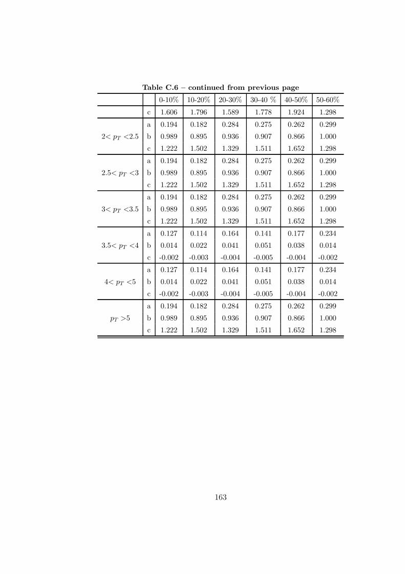
Table C.6 – continued from previous page

0-10% 10-20% 20-30% 30-40 % 40-50% 50-60%

c 1.606 1.796 1.589 1.778 1.924 1.298

2< pT <2.5

a 0.194 0.182 0.284 0.275 0.262 0.299

b 0.989 0.895 0.936 0.907 0.866 1.000

c 1.222 1.502 1.329 1.511 1.652 1.298

2.5< pT <3

a 0.194 0.182 0.284 0.275 0.262 0.299

b 0.989 0.895 0.936 0.907 0.866 1.000

c 1.222 1.502 1.329 1.511 1.652 1.298

3< pT <3.5

a 0.194 0.182 0.284 0.275 0.262 0.299

b 0.989 0.895 0.936 0.907 0.866 1.000

c 1.222 1.502 1.329 1.511 1.652 1.298

3.5< pT <4

a 0.127 0.114 0.164 0.141 0.177 0.234

b 0.014 0.022 0.041 0.051 0.038 0.014

c -0.002 -0.003 -0.004 -0.005 -0.004 -0.002

4< pT <5

a 0.127 0.114 0.164 0.141 0.177 0.234

b 0.014 0.022 0.041 0.051 0.038 0.014

c -0.002 -0.003 -0.004 -0.005 -0.004 -0.002

pT >5

a 0.194 0.182 0.284 0.275 0.262 0.299

b 0.989 0.895 0.936 0.907 0.866 1.000

c 1.222 1.502 1.329 1.511 1.652 1.298

163

164

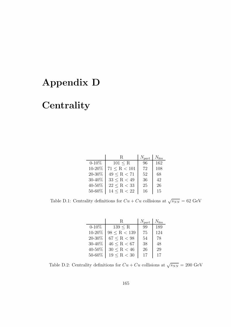
Appendix D

Centrality

R Npart Nbin

0-10% 101 ≤ R 96 16210-20% 71 ≤ R < 101 72 10820-30% 49 ≤ R < 71 52 6830-40% 33 ≤ R < 49 36 4240-50% 22 ≤ R < 33 25 2650-60% 14 ≤ R < 22 16 15

Table D.1: Centrality definitions for Cu+ Cu collisions at√sNN = 62 GeV

R Npart Nbin

0-10% 139 ≤ R 99 18910-20% 98 ≤ R < 139 75 12420-30% 67 ≤ R < 98 54 7830-40% 46 ≤ R < 67 38 4840-50% 30 ≤ R < 46 26 2950-60% 19 ≤ R < 30 17 17

Table D.2: Centrality definitions for Cu+ Cu collisions at√sNN = 200 GeV

165

R Npart Nbin

0-5% 373 ≤ R 347 9045-10% 313 ≤ R < 373 293 71410-20% 222 ≤ R < 313 229 51220-30% 154 ≤ R < 222 162 32130-40% 102 ≤ R < 154 112 19340-50% 65 ≤ R < 102 74 10950-60% 38 ≤ R < 65 46 5760-70% 20 ≤ R < 38 26 2770-80% 9 ≤ R < 20 13 11

Table D.3: Centrality definitions for Au+ Au collisions at√sNN = 62 GeV

166

Bibliography

[1] S. Bethke, Experimental Tests of Asymptotic Freedom, Prog. Part. Nucl. Phys.

58, 351 (2007), hep-ex/0606035.

[2] G. Baym, RHIC: From dreams to beams in two decades, Nucl. Phys. A698,

XXIII (2002), hep-ph/0104138.

[3] N. P. Samios, RHIC: the early years, Journal of Physics G: Nuclear and Particle

Physics 34, S181 (2007).

[4] L. McLerran, T. D. Lee: Relativistic Heavy Ion Collisions and the Riken

Brookhaven Center, (2006).

[5] N. P. Samios and T. W. Ludlam, Future high energy heavy ion physics at

Brookhaven, Nucl. Phys. A 498, 323c (1989).

[6] M. A. Stephanov, QCD phase diagram: An overview, PoS LAT2006, 024

(2006), hep-lat/0701002.

[7] S. D. Bass, How Does the Proton Spin?, Science 315, 1672 (2007).

[8] M. G. Alford, A. Schmitt, K. Rajagopal, and T. Schafer, Color superconductivity

in dense quark matter, Rev. Mod. Phys. 80, 1455 (2008), 0709.4635.

[9] U. M. Heller, Recent progress in finite temperature lattice QCD, PoS LAT2006,

011 (2006), hep-lat/0610114.

[10] M. A. Alford, Color superconductivity in ultra-dense quark matter, PoS

LAT2006, 001 (2006).

167

[11] E. Shuryak, Some thoughts on critical and tricritical points and deconfinement,

PoS CPOD2006, 026 (2006), nucl-th/0609011.

[12] S. Bass, Collision dynamics and cascades, Talk at Quark Matter 2001, 2001.

[13] T. Ullrich, Rhic experimental overview - what we have learned, Talk at Colliders

to Cosmic Rays 2007, 2007.

[14] T. Ullrich, The charm and beauty of an (almost) perfect liquid - open heavy

flavor production at rhic, Seminar given at the NSCL at MSU on February 7,

2007, 2007.

[15] T. Renk, Mach cones and dijets: Jet quenching and fireball expansion dynamics,

(2006), hep-ph/0608333.

[16] S. A. Bass et al., Last call for RHIC predictions, Nucl. Phys. A661, 205 (1999),

nucl-th/9907090.

[17] C. Adler et al. (STAR Collaboration), Centrality dependence of high pT hadron

suppression in Au+Au collisions at√sNN = 130-GeV, Phys. Rev. Lett. 89,

202301 (2002), nucl-ex/0206011.

[18] J. W. Cronin et al., Production of Hadrons with Large Transverse Momentum

at 200-GeV, 300-GeV, and 400-GeV, Phys. Rev. D11, 3105 (1975).

[19] J. Adams et al. (STAR Collaboration), Evidence from d + Au measurements

for final-state suppression of high p(T) hadrons in Au + Au collisions at RHIC,

Phys. Rev. Lett. 91, 072304 (2003), nucl-ex/0306024.

[20] A. Adare et al. (PHENIX Collaboration), Suppression pattern of neutral pions

at high transverse momentum in Au+Au collisions at sqrt(sNN) = 200 GeV

and constraints on medium transport coefficients, Phys. Rev. Lett. 101, 232301

(2008), 0801.4020.

[21] R. Baier and D. Schiff, Deciphering the properties of the medium produced in

heavy ion collisions at RHIC by a pQCD analysis of quenched large p(T) pi0

spectra, JHEP 09, 059 (2006), hep-ph/0605183.

168

[22] K. J. Eskola, H. Honkanen, C. A. Salgado, and U. A. Wiedemann, The fragility

of high-p(T) hadron spectra as a hard probe, Nucl. Phys. A747, 511 (2005),

hep-ph/0406319.

[23] F. Arleo, Tomography of cold and hot QCD matter: Tools and diagnosis. ((V)),

JHEP 11, 044 (2002), hep-ph/0210104.

[24] A. Adare et al. (PHENIX Collaboration), Energy Loss and Flow of Heavy

Quarks in Au+Au Collisions at sqrt(sNN) = 200 GeV, Phys. Rev. Lett. 98,

172301 (2007), nucl-ex/0611018.

[25] L. McLerran, The Color Glass Condensate and Glasma, (2008), 0804.1736.

[26] B. C. Reisert (ZEUS Collaboration), HERA Combined Cross Sections and Par-

ton Densities, (2008), 0809.4946.

[27] F. Becattini, An introduction to the Statistical Hadronization Model, (2009),

0901.3643.

[28] S. Wheaton and J. Cleymans, THERMUS: A thermal model package for ROOT,

Comput. Phys. Commun. 180, 84 (2009), hep-ph/0407174.

[29] J. Adams et al. (STAR Collaboration), Experimental and theoretical challenges

in the search for the quark gluon plasma: The STAR collaboration’s critical

assessment of the evidence from RHIC collisions, Nucl. Phys. A757, 102 (2005),

nucl-ex/0501009.

[30] P. Braun-Munzinger, K. Redlich, and J. Stachel, Particle production in heavy

ion collisions, (2003), nucl-th/0304013.

[31] P. F. Kolb, J. Sollfrank, and U. W. Heinz, Anisotropic transverse flow and

the quark-hadron phase transition, Phys. Rev. C62, 054909 (2000), hep-

ph/0006129.

[32] P. Huovinen, P. F. Kolb, U. W. Heinz, P. V. Ruuskanen, and S. A. Voloshin,

Radial and elliptic flow at RHIC: further predictions, Phys. Lett. B503, 58

(2001), hep-ph/0101136.

169

[33] D. Teaney, J. Lauret, and E. V. Shuryak, A hydrodynamic description of heavy

ion collisions at the SPS and RHIC, (2001), nucl-th/0110037.

[34] T. Hirano, K. Morita, S. Muroya, and C. Nonaka, Hydrodynamical analysis of

hadronic spectra in the 130- GeV/nucleon Au + Au collisions, Phys. Rev. C65,

061902 (2002), nucl-th/0110009.

[35] P. F. Kolb and U. W. Heinz, Hydrodynamic description of ultrarelativistic heavy-

ion collisions, (2003), nucl-th/0305084.

[36] A. Krasnitz, Y. Nara, and R. Venugopalan, Elliptic flow of colored glass in high

energy heavy ion collisions, Phys. Lett. B554, 21 (2003), hep-ph/0204361.

[37] D. Teaney and R. Venugopalan, Classical computation of elliptic flow at large

transverse momentum, Phys. Lett. B539, 53 (2002), hep-ph/0203208.

[38] B. Z. Kopeliovich, A. H. Rezaeian, and I. Schmidt, Azimuthal Asymmetry of

pions in pp and pA collisions, (2008), 0809.4327.

[39] K. G. Boreskov, A. B. Kaidalov, and O. V. Kancheli, Anisotropic flows from

initial state of a fast nucleus, Eur. Phys. J. C58, 445 (2008), 0809.0625.

[40] S. A. Voloshin, A. M. Poskanzer, and R. Snellings, Collective phenomena in

non-central nuclear collisions, (2008), 0809.2949.

[41] M. L. Miller, K. Reygers, S. J. Sanders, and P. Steinberg, Glauber modeling

in high energy nuclear collisions, Ann. Rev. Nucl. Part. Sci. 57, 205 (2007),

nucl-ex/0701025.

[42] A. Adare et al. (PHENIX Collaboration), Scaling properties of azimuthal

anisotropy in Au + Au and Cu + Cu collisions at s(NN)**(1/2) = 200-GeV,

Phys. Rev. Lett. 98, 162301 (2007), nucl-ex/0608033.

[43] B. I. Abelev et al. (STAR Collaboration), Centrality dependence of charged

hadron and strange hadron elliptic flow from√sNN = 200 GeV Au+Au colli-

sions, Phys. Rev. C77, 054901 (2008), 0801.3466.

170

[44] B. I. Abelev et al. (the STAR Collaboration), Mass, quark-number, and

s(NN)**(1/2) dependence of the second and fourth flow harmonics in ultra-

relativistic nucleus nucleus collisions, Phys. Rev. C75, 054906 (2007), nucl-

ex/0701010.

[45] S. Salur, Statistical models and STAR’s strange data, (2006), nucl-ex/0606006.

[46] R. J. Fries, V. Greco, and P. Sorensen, Coalescence Models For Hadron Forma-

tion From Quark Gluon Plasma, (2008), 0807.4939.

[47] M. E. Peskin and D. V. Schroeder, An Introduction to Quantum Field Theory;

1995 ed. (Westview, Boulder, CO, 1995), Includes exercises.

[48] J.-y. Jia, How to Make Sense of the Jet Correlations Results at RHIC?, (2008),

0810.0051.

[49] J. Adams et al. (STAR Collaboration), The energy dependence of p(t) angular

correlations inferred from mean-p(t) fluctuation scale dependence in heavy ion

collisions at the SPS and RHIC, J. Phys. G33, 451 (2007), nucl-ex/0605021.

[50] J. Adams et al. (STAR Collaboration), Direct observation of dijets in central

Au + Au collisions at s(NN)**(1/2) = 200-GeV, Phys. Rev. Lett. 97, 162301

(2006), nucl-ex/0604018.

[51] J. Adams et al. (STAR Collaboration), Distributions of charged hadrons as-

sociated with high transverse momentum particles in p p and Au + Au colli-

sions at s(NN)**(1/2) = 200-GeV, Phys. Rev. Lett. 95, 152301 (2005), nucl-

ex/0501016.

[52] J. Adams et al. (STAR Collaboration), Azimuthal anisotropy and correlations

at large transverse momenta in p + p and Au + Au collisions at s(NN)**(1/2)

= 200-GeV, Phys. Rev. Lett. 93, 252301 (2004), nucl-ex/0407007.

[53] J. Adams et al. (STAR Collaboration), Evidence from d + Au measurements

for final-state suppression of high p(T) hadrons in Au + Au collisions at RHIC,

Phys. Rev. Lett. 91, 072304 (2003), nucl-ex/0306024.

171

[54] C. Adler et al. (STAR Collaboration), Disappearance of back-to-back high p(T)

hadron correlations in central Au + Au collisions at s(NN)**(1/2) = 200-GeV,

Phys. Rev. Lett. 90, 082302 (2003), nucl-ex/0210033.

[55] C. Adler et al. (STAR Collaboration), Azimuthal anisotropy and correlations

in the hard scattering regime at RHIC, Phys. Rev. Lett. 90, 032301 (2003),

nucl-ex/0206006.

[56] S. Afanasiev et al. (PHENIX Collaboration), Particle-species dependent modi-

fication of jet-induced correlations in Au+Au collisions at s(NN)**(1/2) = 200

GeV, Phys. Rev. Lett. 101, 082301 (2008), 0712.3033.

[57] A. Adare et al. (PHENIX Collaboration), Dihadron azimuthal correlations in

Au+Au collisions at sqrts(NN)**(1/2) = 200 GeV, Phys. Rev. C78, 014901

(2008), 0801.4545.

[58] A. Adare et al. (PHENIX Collaboration), Transverse momentum and centrality

dependence of dihadron correlations in Au+Au collisions at s(NN)**(1/2)=200

GeV: Jet-quenching and the response of partonic matter, Phys. Rev. C77,

011901 (2008), 0705.3238.

[59] A. Adare et al. (PHENIX Collaboration), System size and energy dependence of

jet-induced hadron pair correlation shapes in Cu + Cu and Au + Au collisions at

s(NN)**(1/2) = 200-GeV and 62.4-GeV, Phys. Rev. Lett. 98, 232302 (2007),

nucl-ex/0611019.

[60] S. S. Adler et al. (PHENIX Collaboration), Jet properties from dihadron cor-

relations in p + p collisions at s**(1/2) = 200-GeV, Phys. Rev. D74, 072002

(2006), hep-ex/0605039.

[61] S. S. Adler et al. (PHENIX Collaboration), Modifications to di-jet hadron pair

correlations in Au + Au collisions at s(NN)**(1/2) = 200-GeV, Phys. Rev.

Lett. 97, 052301 (2006), nucl-ex/0507004.

172

[62] S. S. Adler et al. (PHENIX Collaboration), Jet structure from dihadron cor-

relations in d + Au collisions at s(NN)**(1/2) = 200-GeV, Phys. Rev. C73,

054903 (2006), nucl-ex/0510021.

[63] M. J. Horner (STAR Collaboration), Azimuthal di-hadron correlations in Au +

Au collisions at s(NN)**(1/2) = 200-GeV from STAR, AIP Conf. Proc. 842,

125 (2006), nucl-ex/0606025.

[64] N. Borghini, Momentum conservation and correlation analyses in heavy- ion

collisions at ultrarelativistic energies, Phys. Rev. C75, 021904 (2007), nucl-

th/0612093.

[65] N. Armesto, C. A. Salgado, and U. A. Wiedemann, Measuring the collective

flow with jets, Phys. Rev. Lett. 93, 242301 (2004), hep-ph/0405301.

[66] V. Koch, A. Majumder, and X.-N. Wang, Cherenkov Radiation from Jets in

Heavy-ion Collisions, Phys. Rev. Lett. 96, 172302 (2006), nucl-th/0507063.

[67] J. Hofmann, H. Stocker, U. Heinz, W. Scheid, and W. Greiner, Possibility of

Detecting Density Isomers in High-Density Nuclear Mach Shock Waves, Phys.

Rev. Lett. 36, 88 (1975).

[68] J. Casalderrey-Solana and E. V. Shuryak, Conical flow in a medium with vari-

able speed of sound, (2005), hep-ph/0511263.

[69] J. G. Ulery, Conical Emission in Heavy Ion Collisions, J. Phys. G35, 104032

(2008), 0807.1613.

[70] J. G. Ulery, Two- and Three-Particle Jet-Like Correlations, (2008), 0801.4904.

[71] J. G. Ulery (STAR Collaboration), Three-Particle Azimuthal Correlations,

Nucl. Phys. A783, 511 (2007), nucl-ex/0609047.

[72] C. A. Pruneau, Three-particle cumulant Study of Conical Emission, (2008),

0810.1461.

173

[73] C. Pruneau (STAR Collaboration), Search for Conical Emission with Three-

Particle Correlations, (2007), nucl-ex/0703010.

[74] J. Putschke (STAR Collaboration), Intra-jet correlations of high-p(t) hadrons

from STAR, J. Phys. G 34, 679 (2007).

[75] M. P. McCumber and f. t. P. Collaboration, The ’Shoulder’ and the ’Ridge’ in

PHENIX, J. Phys. G35, 104081 (2008), 0804.4319.

[76] B. Alver et al. (PHOBOS Collaboration), High pT Triggered Delta-eta,Delta-phi

Correlations over a Broad Range in Delta-eta, J. Phys. G35, 104080 (2008),

0804.3038.

[77] J. Bielcikova (STAR Collaboration), Azimuthal and pseudo-rapidity correlations

with strange particles at intermediate-p(T) at RHIC, J. Phys. G34, S929 (2007),

nucl-ex/0701047.

[78] X.-N. Wang, High-pT Hadron Spectra, Azimuthal Anisotropy and Back- to-

Back Correlations in High-energy Heavy-ion Collisions, Phys. Lett. B595, 165

(2004), nucl-th/0305010.

[79] J. Bielcikova (STAR Collaboration), Two-particle correlations with strange

baryons and mesons at RHIC, (2007), 0707.3100.

[80] C. Suarez, Particle dependence of the ridge and the jet, Poster given at Quark

Matter 2008, 2008.

[81] B. I. Abelev (STAR Collaboration), Multi-strange baryon correlations at RHIC,

(2007), 0705.3371.

[82] A. Feng (STAR Collaboration), Reaction Plane Dependent Away-side Modifica-

tion and Near-side Ridge in Au+Au Collisions, J. Phys. G 35, 104082 (2008).

[83] P. K. Netrakanti (STAR Collaboration), Identifying the underlying physics of

the ridge via 3- particle ∆η − ∆η correlations, J. Phys. G35, 104010 (2008),

0804.4417.

174

[84] M. Daugherity (STAR Collaboration), Anomalous centrality variation of mini-

jet angular correlations in Au-Au collisions at 62 and 200 GeV from STAR, J.

Phys. G35, 104090 (2008), 0806.2121.

[85] S. Salur (STAR Collaboration), A Short Review on Jet Identification, nucl-

ex/0810.0500.

[86] B. I. Abelev et al. (STAR Collaboration), Longitudinal double-spin asymmetry

for inclusive jet production in p+p collisions at sqrt(s)=200 GeV, Phys. Rev.

Lett. 100, 232003 (2008), 0710.2048.

[87] M. Cacciari, G. P. Salam, and G. Soyez, The Catchment Area of Jets, JHEP

04, 005 (2008), 0802.1188.

[88] M. Cacciari, FastJet: A Code for fast kt clustering, and more, (2006), hep-

ph/0607071.

[89] S. Salur (STAR Collaboration), Searching for Jets in Heavy Ion Collisions,

nucl-ex/0809.1606.

[90] J. Putschke (STAR Collaboration), Searching for Jets in Heavy Ion Collisions,

nucl-ex/0809.1419.

[91] S. Salur (STAR Collaboration), First Direct Measurement of Jets in√sNN =

200 GeV Heavy Ion Collisions by STAR, nucl-ex/0809.1609.

[92] T. Ullrich, Rhic: From colliding ions to physics results, Series of lectures

presented at the QCD school in Les Houches, France, 2008.

[93] M. Anderson, T. Ludlam, and S. Ozaki, RHIC project overview, Nucl. Instrum.

Meth. A 499, 235 (2003).

[94] K. H. Ackermann et al., STAR detector overview, Nucl. Instrum. Meth. A 499,

624 (2003).

175

[95] M. Anderson et al., The STAR time projection chamber: a unique tool for

studying high multiplicity events at RHIC, Nucl. Instrum. Meth. A 499, 659

(2003).

[96] G. Van Buren, private communication, 2009.

[97] M. Anderson et al., A readout system for the STAR time projection chamber,

Nucl. Instrum. Meth. A 499, 679 (2003).

[98] W.-M. Yao et al., Review of Particle Physics, Journal of Physics G 33, 1+

(2006).

[99] S. Sevil, Investigation of Hadronic Resonances with STAR, PhD thesis, Yale,

2006.

[100] P. Maybeck, Stochastic models, estimation, and control Volume 1 (Academic

Press, 1979).

[101] B. I. Abelev et al. (STAR Collaboration), Forward Λ Production and Nuclear

Stopping Power in d + Au Collisions at√sNN = 200 GeV, Phys. Rev. C76,

064904 (2007), 0706.0472.

[102] B. I. Abelev et al. (STAR Collaboration), Enhanced strange baryon production

in Au+Au collisions compared to p+p at sqrts = 200 GeV, Phys. Rev. C77,

044908 (2008), 0705.2511.

[103] B. I. Abelev et al. (the STAR Collaboration), Mass, quark-number, and

s(NN)**(1/2) dependence of the second and fourth flow harmonics in ultra-

relativistic nucleus nucleus collisions, Phys. Rev. C75, 054906 (2007), nucl-

ex/0701010.

[104] B. I. Abelev et al. (STAR Collaboration), Neutral kaon interferometry in Au

+ Au collisions at s(NN)**(1/2) = 200-GeV, Phys. Rev. C74, 054902 (2006),

nucl-ex/0608012.

176

[105] B. I. Abelev et al. (STAR Collaboration), Strange particle production in p +

p collisions at s**(1/2) = 200-GeV, Phys. Rev. C75, 064901 (2007), nucl-

ex/0607033.

[106] J. Adams et al. (STAR Collaboration), Scaling Properties of Hyperon Produc-

tion in Au+Au Collisions at sqrt(sNN) = 200 GeV, Phys. Rev. Lett. 98,

062301 (2007), nucl-ex/0606014.

[107] J. Adams et al. (STAR Collaboration), Proton Lambda correlations in central

Au + Au collisions at s(NN)**(1/2) = 200-GeV, Phys. Rev. C74, 064906

(2006), nucl-ex/0511003.

[108] J. Adams et al. (STAR Collaboration), Multi-strange baryon elliptic flow in

Au + Au collisions at s(NN)**(1/2) = 200-GeV, Phys. Rev. Lett. 95, 122301

(2005), nucl-ex/0504022.

[109] J. Adams et al. (STAR Collaboration), Multi-strange baryon production in Au

Au collisions at s(NN)**(1/2) = 130-GeV, Phys. Rev. Lett. 92, 182301 (2004),

nucl-ex/0307024.

[110] J. Adams et al. (STAR Collaboration), Particle dependence of azimuthal

anisotropy and nuclear modification of particle production at moderate p(T) in

Au + Au collisions at s(NN)**(1/2) = 200-GeV, Phys. Rev. Lett. 92, 052302

(2004), nucl-ex/0306007.

[111] C. Adler et al. (STAR Collaboration), Kaon production and kaon to pion ratio

in Au + Au collisions at s(NN)**(1/2) = 130-GeV, Phys. Lett. B595, 143

(2004), nucl-ex/0206008.

[112] C. Adler et al. (STAR Collaboration), Azimuthal anisotropy of K0(S) and

Lambda + anti-Lambda production at mid-rapidity from Au + Au collisions at

s(NN)**(1/2) = 130-GeV, Phys. Rev. Lett. 89, 132301 (2002), hep-ex/0205072.

[113] C. Adler et al. (STAR Collaboration), Mid-rapidity Lambda and Antilambda

production in Au + Au collisions at s(NN)**(1/2) = 130-GeV, Phys. Rev.

Lett. 89, 092301 (2002), nucl-ex/0203016.

177

[114] W. M. Yao et al. (Particle Data Group Collaboration), Review of particle

physics, J. Phys. G33, 1 (2006).

[115] Y. Guo, Identified Particle Correlations At Intermediate Transverse Momentum

In Relativistic Heavy Ion Collisions, PhD thesis, Wayne State University, 2005.

[116] S. Galliard, A study of jets at the STAR experiment at the Relativistic Heavy

Ion Collider vi two-particle correlations, PhD thesis, University of Birmingham,

2008.

[117] J. Bielcikova (STAR Collaboration), Medium properties and jet-medium inter-

action from STAR, (2008), 0806.2261.

[118] J. Bielcikova (STAR Collaboration), High-p(T) strange particle spectra and cor-

relations in STAR, Nucl. Phys. A783, 565 (2007), nucl-ex/0612028.

[119] J. Bielcikova (STAR Collaboration), High-p(T) azimuthal correlations of neutral

strange baryons and mesons in STAR at RHIC, AIP Conf. Proc. 842, 53 (2006),

nucl-ex/0603008.

[120] M. Bombara (STAR Collaboration), Is there a strange baryon / meson depen-

dence in correlations in STAR?, J. Phys. G35, 044065 (2008).

[121] Y. Guo (STAR Collaboration), Identified particle correlation studies in central

Au + Au collisions at s(NN)**(1/2) = 200-GeV, J. Phys. G31, S549 (2005),

nucl-ex/0502015.

[122] Y. Guo (STAR Collaboration), Identified high p(T) particle correlation stud-

ies in central Au + Au collisions at s(NN)**(1/2) = 200-GeV, (2004), hep-

ex/0403018.

[123] B. Abelev, Multi-Strange Baryon Correlations at RHIC, PhD thesis, Yale,

2007.

[124] A. Iordanova (STAR Collaboration), Particle Production at RHIC, (2008),

0806.0286.

178

[125] M. Estienne, Proprits chimiques et dynamiques des collisions d’ions lourds aux

nergies du RHIC par la mesure de la production des baryons doublement tranges

dans l’exprience STAR, PhD thesis, SUBATECH, 2005.

[126] A. Timmins, Neutral Strange Particle Production in Relativistic Cu+Cu Colli-

sions at√sNN = 200 GeV, PhD thesis, University of Birmingham, 2008.

[127] J. Adams et al. (STAR Collaboration), Pion interferometry in Au + Au col-

lisions at s(NN)**(1/2) = 200-GeV, Phys. Rev. C71, 044906 (2005), nucl-

ex/0411036.

[128] B. B. Back et al. (PHOBOS Collaboration), Centrality and pseudorapidity

dependence of elliptic flow for charged hadrons in Au + Au collisions at

s(NN)**(1/2) = 200-GeV, Phys. Rev. C72, 051901 (2005), nucl-ex/0407012.

[129] B. B. Back et al. (PHOBOS Collaboration), Energy dependence of elliptic flow

over a large pseudorapidity range in Au + Au collisions at RHIC, Phys. Rev.

Lett. 94, 122303 (2005), nucl-ex/0406021.

[130] J. Adams et al. (STAR Collaboration), FILL IN THE NAME OF OANA’S

PAPER, CHECKME WRONG, 451 (2007), nucl-ex/0605021.

[131] J. Adams et al. (STAR Collaboration), FILL IN THE NAME OF JOERN’S

RIDGE PAPER, CHECKME WRONG, 451 (2007), nucl-ex/0605021.

[132] J. Bielcikova, S. Esumi, K. Filimonov, S. Voloshin, and J. P. Wurm, Elliptic flow

contribution to two-particle correlations at different orientations to the reaction

plane, Phys. Rev. C69, 021901 (2004), nucl-ex/0311007.

[133] S. A. Voloshin (STAR Collaboration), Energy and system size dependence of

charged particle elliptic flow and v(2)/epsilon scaling, J. Phys. G34, S883

(2007), nucl-ex/0701038.

[134] J. Adams et al. (STAR Collaboration), Azimuthal anisotropy and correlations

at large transverse momenta in p + p and Au + Au collisions at s(NN)**(1/2)

= 200-GeV, Phys. Rev. Lett. 93, 252301 (2004), nucl-ex/0407007.

179

[135] A. Tang, private communication, 2007.

[136] S. Shi (STAR Collaboration), Strange hadron elliptic flow from 200 GeV Cu+Cu

collisions, (2008), 0806.0763.

[137] J. Bielcikova, Private communication, 2007-2009.

[138] B. Abelev, Multi-Strange Baryon Correlations at RHIC, PhD thesis, Yale

University, 2007.

[139] A. R. Timmins (STAR Collaboration), The Centrality Dependence of Strange

Baryon and Meson Production in Cu+Cu and Au+Au sqrt(sNN) = 200 GeV

collisions, Int. J. Mod. Phys. E16, 2055 (2007), 0708.3290.

[140] M. A. C. Lamont (STAR Collaboration), Identified particles at large transverse

momenta in STAR in Au + Au collisions at s(NN)**(1/2) = 200-GeV, J. Phys.

G30, S963 (2004), nucl-ex/0403059.

[141] T. Sjostrand, L. Lonnblad, S. Mrenna, and P. Skands, Pythia 6.3 physics and

manual, (2003), hep-ph/0308153.

[142] R. D. Field (CDF Collaboration), The underlying event in hard scattering pro-

cesses, (2002), hep-ph/0201192.

[143] J. Adams et al. (STAR Collaboration), The Multiplicity dependence of inclusive

pt spectra from pp collisions at√s = 200-GeV, Phys. Rev. D74, 032006 (2006),

nucl-ex/0606028.

[144] J. Adams et al. (STAR Collaboration), Identified hadron spectra at large trans-

verse momentum in p + p and d + Au collisions at s(NN)**(1/2) = 200-GeV,

Phys. Lett. B637, 161 (2006), nucl-ex/0601033.

[145] S. A. Voloshin, Anisotropic collective phenomena in ultra-relativistic nuclear

collisions, (2009), 0902.0581.

180

[146] C. A. Pruneau, S. Gavin, and S. A. Voloshin, Transverse Radial Flow Effects on

Two- and Three-Particle Angular Correlations, Nucl. Phys. A802, 107 (2008),

0711.1991.

[147] J. Takahashi et al., Topology studies of hydrodynamics using two particle corre-

lation analysis, (2009), 0902.4870.

[148] E. V. Shuryak, On the Origin of the ’Ridge’ phenomenon induced by Jets in

Heavy Ion Collisions, Phys. Rev. C76, 047901 (2007), 0706.3531.

[149] A. Dumitru, F. Gelis, L. McLerran, and R. Venugopalan, Glasma flux tubes

and the near side ridge phenomenon at RHIC, Nucl. Phys. A810, 91 (2008),

0804.3858.

[150] F. Gelis, T. Lappi, and R. Venugopalan, High energy factorization and long

range rapidity correlations in the Glasma, (2008), 0810.4829.

[151] R. Mizukawa et al., Search for a Ridge Structure Origin with Shower Broadening

and Jet Quenching, J. Phys. G 35, 104083 (2008).

[152] S. Gavin, L. McLerran, and G. Moschelli, Long Range Correlations and the Soft

Ridge in Relativistic Nuclear Collisions, (2008), 0806.4718.

[153] R. C. Hwa and C. B. Yang, Production of strange particles at intermediate p(T)

at RHIC, (2006), nucl-th/0602024.

[154] C. B. Chiu and R. C. Hwa, Particles Associated with Omega Produced at Inter-

mediate pT, Phys. Rev. C76, 024904 (2007), 0704.2616.

[155] R. C. Hwa, Hadron Correlations in Jets and Ridges through Parton Recombi-

nation, (2009), 0904.2159.

[156] C. B. Chiu and R. C. Hwa, Dependence of Ridge Formation on Trigger Azimuth:

Correlated Emission Model, (2008), 0809.3018.

[157] C. yin Wong, Ridge Structure associated with the Near-Side Jet in the (Delta

phi)-(Delta eta) Correlation, Phys. Rev. C 76, 054908 (2007).

181

[158] C. yin Wong, private communication, 2008.

[159] C. yin Wong, The Momentum Kick Model Description of the Near-Side Ridge

and Jet Quenching, hep-ph/0806.2154.

[160] A. Majumder, B. Muller, and S. A. Bass, Longitudinal Broadening of Quenched

Jets in Turbulent Color Fields, Phys. Rev. Lett. 99, 042301 (2007), hep-

ph/0611135.

[161] H. Crawford, Star future plans and upgrades, Presented at 2009 RHIC/AGS

User’s Meeting, 2009.

[162] J. Putschke (STAR Collaboration), First fragmentation function measurements

from full jet reconstruction in heavy-ion collisions at√s

NN= 200 GeV by STAR,

(2008), 0809.1419.

[163] M. Szuba (NA49 Collaboration), Energy and System-size Dependence of Two-

particle Azimuthal Correlations of High-pT Charged Hadrons at the CERN SPS,

(2008), 0809.5210.

[164] M. Szuba and f. t. N. Collaboration, Two-particle Azimuthal Correlations of

High-pT Charged Hadrons at the CERN SPS, (2008), 0805.4637.

182