1

Categorical Principal Components Analysis (CATPCA)

SPSS is a registered trademark and the other product names are the trademarks of SPSS Inc. for its proprietary computersoftware. No material describing such software may be produced or distributed without the written permission of the ownersof the trademark and license rights in the software and the copyrights in the published materials.

The SOFTWARE and documentation are provided with RESTRICTED RIGHTS. Use, duplication, or disclosure by theGovernment is subject to restrictions as set forth in subdivision (c)(1)(ii) of The Rights in Technical Data and ComputerSoftware clause at 52.227-7013. Contractor/manufacturer is SPSS Inc., 233 South Wacker Drive, 11th Floor, Chicago, IL60606-6307.

General notice: Other product names mentioned herein are used for identification purposes only and may be trademarks oftheir respective companies.

TableLook is a trademark of SPSS Inc.Windows is a registered trademark of Microsoft Corporation.ImageStream ® Graphics & Presentation Filters, copyright© 1991-1999 by INSO Corporation. All Rights Reserved.ImageStream Graphics Filters is a registered trademark and ImageStream is a trademark of INSO Corporation.

DataDirect, INTERSOLV, and SequeLink are registered trademarks of MERANT Solutions Inc.DataDirect Connect is a trademark of MERANT Solutions Inc.

Copyright © 1999 by SPSS Inc.All rights reserved.Printed in the United States of America.

No part of this publication may be reproduced, stored in a retrieval system, or transmitted, in any form or by any means,electronic, mechanical, photocopying, recording, or otherwise, without the prior written permission of the publisher.

2

CATPCA

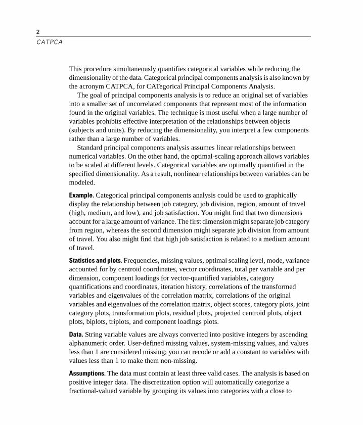
This procedure simultaneously quantifies categorical variables while reducing the dimensionality of the data. Categorical principal components analysis is also known by the acronym CATPCA, for CATegorical Principal Components Analysis.

The goal of principal components analysis is to reduce an original set of variables into a smaller set of uncorrelated components that represent most of the information found in the original variables. The technique is most useful when a large number of variables prohibits effective interpretation of the relationships between objects (subjects and units). By reducing the dimensionality, you interpret a few components rather than a large number of variables.

Standard principal components analysis assumes linear relationships between numerical variables. On the other hand, the optimal-scaling approach allows variables to be scaled at different levels. Categorical variables are optimally quantified in the specified dimensionality. As a result, nonlinear relationships between variables can be modeled.

Example. Categorical principal components analysis could be used to graphically display the relationship between job category, job division, region, amount of travel (high, medium, and low), and job satisfaction. You might find that two dimensions account for a large amount of variance. The first dimension might separate job category from region, whereas the second dimension might separate job division from amount of travel. You also might find that high job satisfaction is related to a medium amount of travel.

Statistics and plots. Frequencies, missing values, optimal scaling level, mode, variance accounted for by centroid coordinates, vector coordinates, total per variable and per dimension, component loadings for vector-quantified variables, category quantifications and coordinates, iteration history, correlations of the transformed variables and eigenvalues of the correlation matrix, correlations of the original variables and eigenvalues of the correlation matrix, object scores, category plots, joint category plots, transformation plots, residual plots, projected centroid plots, object plots, biplots, triplots, and component loadings plots.

Data. String variable values are always converted into positive integers by ascending alphanumeric order. User-defined missing values, system-missing values, and values less than 1 are considered missing; you can recode or add a constant to variables with values less than 1 to make them non-missing.

Assumptions. The data must contain at least three valid cases. The analysis is based on positive integer data. The discretization option will automatically categorize a fractional-valued variable by grouping its values into categories with a close to

3

CATPCA

“normal” distribution and will automatically convert values of string variables into positive integers. You can specify other discretization schemes.

Related procedures. Scaling all variables at the numerical level corresponds to standard principal components analysis. Alternate plotting features are available by using the transformed variables in a standard linear principal components analysis. If all variables have multiple nominal scaling levels, categorical principal components analysis is identical to homogeneity analysis. If sets of variables are of interest, categorical (nonlinear) canonical correlation analysis should be used.

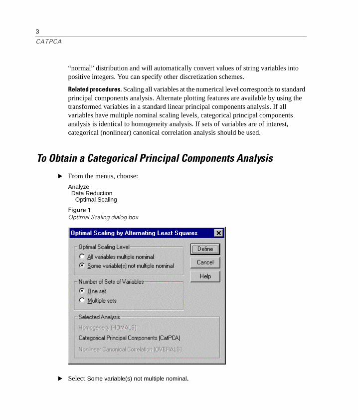
To Obtain a Categorical Principal Components Analysis � From the menus, choose:

AnalyzeData Reduction

Optimal Scaling

Figure 1Optimal Scaling dialog box

� Select Some variable(s) not multiple nominal.

4

CATPCA

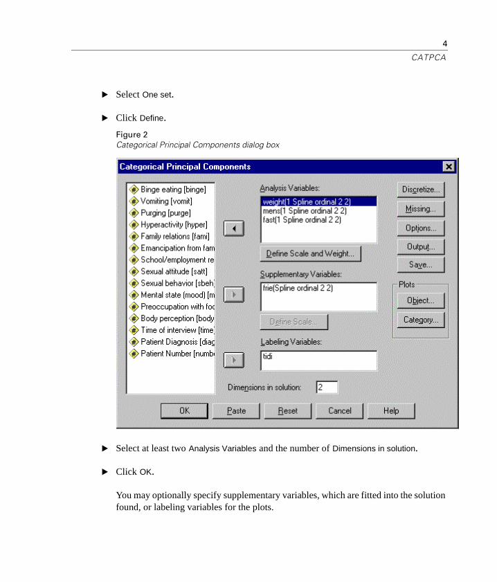
� Select One set.

� Click Define.

Figure 2Categorical Principal Components dialog box

� Select at least two Analysis Variables and the number of Dimensions in solution.

� Click OK.

You may optionally specify supplementary variables, which are fitted into the solution found, or labeling variables for the plots.

5

CATPCA

Define Scale and Weight in CATPCA

You can set the optimal scaling level for analysis variables and supplementary variables. By default, they are scaled as second-degree monotonic splines (ordinal) with two interior knots. Additionally, you can set the weight for analysis variables.

Variable weight. You can choose to define a weight for each variable. The value specified must be a positive integer. The default value is 1.

Optimal scaling level. You can also select the scaling level to be used to quantify each variable.

n Spline ordinal. The order of the categories of the observed variable is preserved in the optimally scaled variable. Category points will be on a straight line (vector) through the origin. The resulting transformation is a smooth monotonic piecewise polynomial of the chosen Degree. The pieces are specified by the user-specified number and procedure-determined placement of the Interior knots.

n Spline nominal. The only information in the observed variable that is preserved in the optimally scaled variable is the grouping of objects in categories. The order of the categories of the observed variable is not preserved. Category points will be on a straight line (vector) through the origin. The resulting transformation is a smooth, possibly non-monotonic, piecewise polynomial of the chosen Degree. The pieces are specified by the user-specified number and procedure-determined placement of the Interior knots.

n Multiple nominal. The only information in the observed variable that is preserved in the optimally scaled variable is the grouping of objects in categories. The order of the categories of the observed variable is not preserved. Category points will be in the centroid of the objects in the particular categories. Multiple indicates that different sets of quantifications are obtained for each dimension.

n Ordinal. The order of the categories of the observed variable is preserved in the optimally scaled variable. Category points will be on a straight line (vector) through the origin. The resulting transformation fits better than the spline ordinal transformation but is less smooth.

n Nominal. The only information in the observed variable that is preserved in the optimally scaled variable is the grouping of objects in categories. The order of the categories of the observed variable is not preserved. Category points will be on a straight line (vector) through the origin. The resulting transformation fits better than the spline nominal transformation but is less smooth.

6

CATPCA

n Numerical. Categories are treated as ordered and equally spaced (interval level). The order of the categories and the equal distances between category numbers of the observed variable are preserved in the optimally scaled variable. Category points will be on a straight line (vector) through the origin. When all variables are at the numerical level, the analysis is analogous to standard principal components analysis.

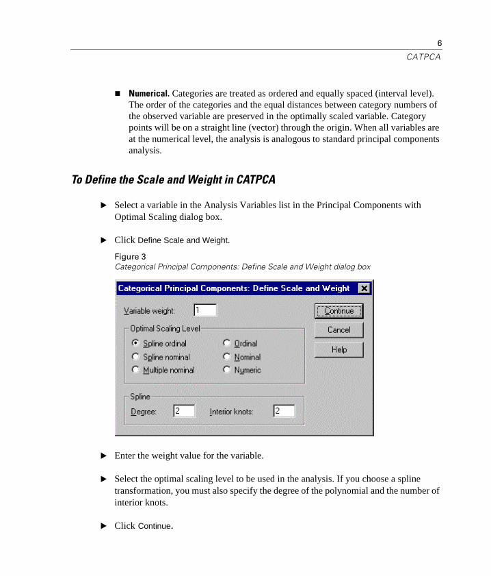
To Define the Scale and Weight in CATPCA

� Select a variable in the Analysis Variables list in the Principal Components with Optimal Scaling dialog box.

� Click Define Scale and Weight.

Figure 3Categorical Principal Components: Define Scale and Weight dialog box

� Enter the weight value for the variable.

� Select the optimal scaling level to be used in the analysis. If you choose a spline transformation, you must also specify the degree of the polynomial and the number of interior knots.

� Click Continue.

7

CATPCA

You can alternately define the scaling level for supplementary variables by selecting them from the list and clicking Define Scale.

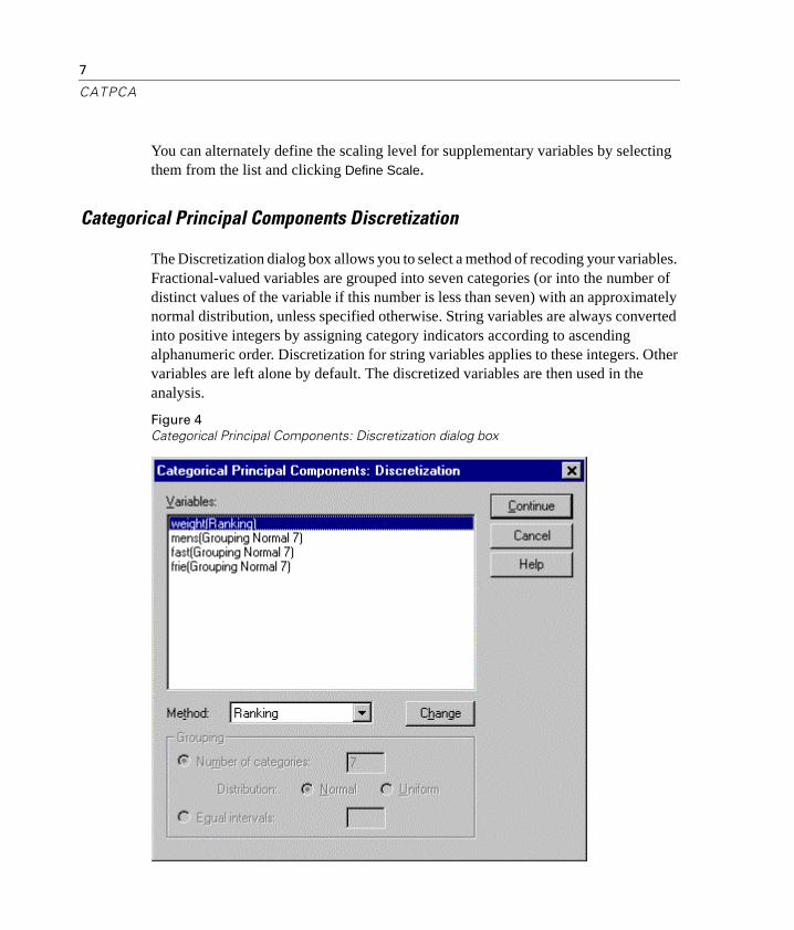
Categorical Principal Components Discretization

The Discretization dialog box allows you to select a method of recoding your variables. Fractional-valued variables are grouped into seven categories (or into the number of distinct values of the variable if this number is less than seven) with an approximately normal distribution, unless specified otherwise. String variables are always converted into positive integers by assigning category indicators according to ascending alphanumeric order. Discretization for string variables applies to these integers. Other variables are left alone by default. The discretized variables are then used in the analysis.

Figure 4Categorical Principal Components: Discretization dialog box

8

CATPCA

Method. Choose between Grouping, Ranking, and Multiplying.

n Grouping. Recode into a specified number of categories or recode by interval.

n Ranking. The variable is discretized by ranking the cases.

n Multiplying. The current values of the variable are standardized, multiplied by 10, rounded, and have a constant added such that the lowest discretized value is 1.

Grouping. You have the following options when discretizing variables by grouping:

n Number of categories. Specify a number of categories and whether the values of the variable should follow an approximately Normal or Uniform distribution across those categories.

n Equal intervals. Variables are recoded into categories defined by these equally sized intervals. You must specify the length of the intervals.

Categorical Principal Components Missing Values

The Missing Values dialog box allows you to choose the strategy for handling missing values in analysis variables and supplementary variables.

9

CATPCA

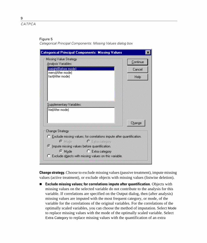
Figure 5Categorical Principal Components: Missing Values dialog box

Change strategy. Choose to exclude missing values (passive treatment), impute missing values (active treatment), or exclude objects with missing values (listwise deletion).

n Exclude missing values; for correlations impute after quantification. Objects with missing values on the selected variable do not contribute to the analysis for this variable. If correlations are specified on the Output dialog, then (after analysis) missing values are imputed with the most frequent category, or mode, of the variable for the correlations of the original variables. For the correlations of the optimally scaled variables, you can choose the method of imputation. Select Mode to replace missing values with the mode of the optimally scaled variable. Select Extra Category to replace missing values with the quantification of an extra

10

CATPCA

category. This implies that objects with a missing value on this variable are considered to belong to the same (extra) category.

n Impute missing values before quantification. Objects with missing values on the selected variable have those values imputed. You can choose the method of imputation. Select Mode to replace missing values with the most frequent category. When there are multiple modes, the one with the smallest category indicator is used. Select Extra Category to replace missing values with the same quantification of an extra category. This implies that objects with a missing value on this variable are considered to belong to the same (extra) category.

n Exclude objects with missing values on this variable. Objects with missing values on the selected variable are excluded from the analysis. This strategy is not available for supplementary variables.

Categorical Principal Components Category Plots

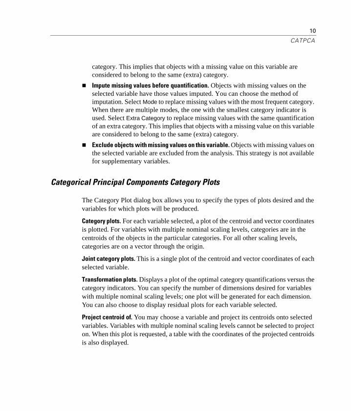
The Category Plot dialog box allows you to specify the types of plots desired and the variables for which plots will be produced.

Category plots. For each variable selected, a plot of the centroid and vector coordinates is plotted. For variables with multiple nominal scaling levels, categories are in the centroids of the objects in the particular categories. For all other scaling levels, categories are on a vector through the origin.

Joint category plots. This is a single plot of the centroid and vector coordinates of each selected variable.

Transformation plots. Displays a plot of the optimal category quantifications versus the category indicators. You can specify the number of dimensions desired for variables with multiple nominal scaling levels; one plot will be generated for each dimension. You can also choose to display residual plots for each variable selected.

Project centroid of. You may choose a variable and project its centroids onto selected variables. Variables with multiple nominal scaling levels cannot be selected to project on. When this plot is requested, a table with the coordinates of the projected centroids is also displayed.

11

CATPCA

To Obtain Category Plots in CATPCAFigure 6Categorical Principal Components: Category Plots dialog box

� Select the types of plots and variables for which plots will be produced.

� Click Continue.

Categorical Principal Components Object and Variable Plots

The Object and Variable Plot dialog box allows you to specify the types of plots desired and the variables for which plots will be produced.

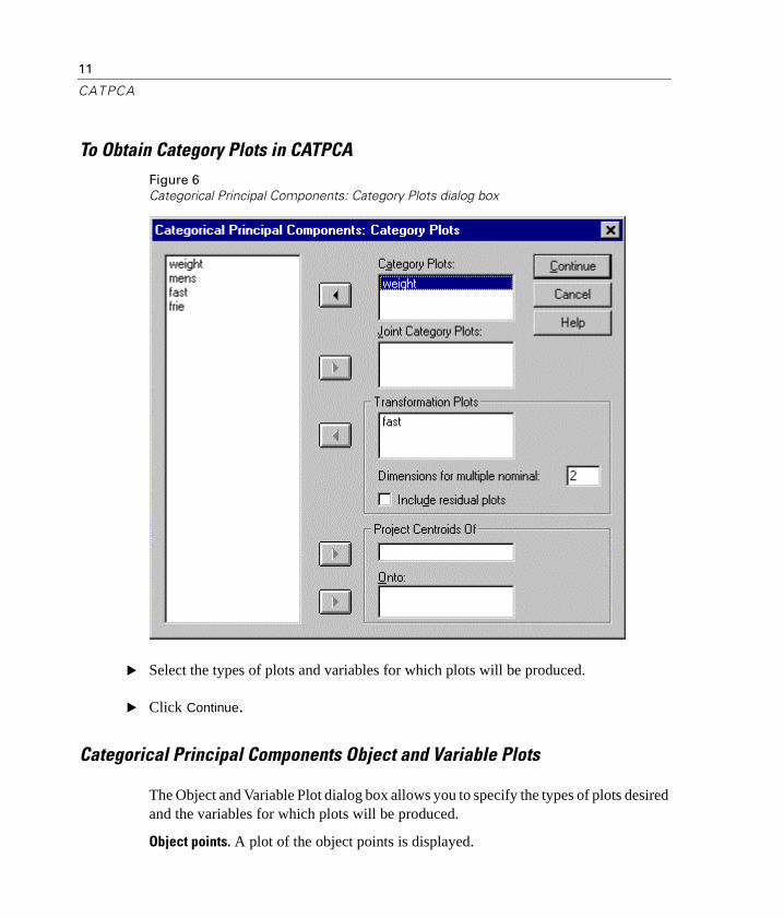
Object points. A plot of the object points is displayed.

12

CATPCA

Objects and variables (biplot). The object points are plotted with your choice of the variable coordinates: component loadings or variable centroids.

Objects, loadings, and centroids (triplot). The object points are plotted with the centroids of multiple nominal scaling-level variables and the component loadings of other variables.

Component loadings. A plot of the component loadings is displayed. Variables with multiple nominal scaling levels do not have component loadings, but you may choose to include the centroids of those variables in the plot.

Biplot and triplot variables. You can choose to use all variables for the biplots and triplots, or select a subset.

Label objects. You can choose to have objects labeled with the categories of selected variables (you may choose category indicator values or value labels in the Options dialog box) or with their case numbers. One plot is produced per variable, if Variables is specified.

13

CATPCA

To Obtain Object and Variable Plots in CATPCAFigure 7Categorical Principal Components: Object and Variable Plots dialog box

� Select the types of plots and variables for which plots will be produced and variables to label the objects in the plot.

� Click Continue.

14

CATPCA

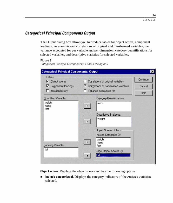
Categorical Principal Components Output

The Output dialog box allows you to produce tables for object scores, component loadings, iteration history, correlations of original and transformed variables, the variance accounted for per variable and per dimension, category quantifications for selected variables, and descriptive statistics for selected variables.

Figure 8Categorical Principal Components: Output dialog box

Object scores. Displays the object scores and has the following options:

n Include categories of. Displays the category indicators of the Analysis Variables selected.

15

CATPCA

n Label object scores by. From the list of variables specified as Labeling Variables, you can select one to label the objects.

Component loadings. Displays the component loadings for all variables that were not given multiple nominal scaling level.

Iteration history. For each iteration, the variance accounted for, loss, and increase in variance accounted for are shown.

Correlations of original variables. Shows the correlation matrix of the original variables and the eigenvalues of that matrix.

Correlations of transformed variables. Shows the correlation matrix of the transformed (optimally scaled) variables and the eigenvalues of that matrix.

Variance accounted for. Displays the amount of variance accounted for by centroid coordinates, vector coordinates, and total (centroid and vector coordinates combined) per variable and per dimension.

Category quantifications. Gives the category quantifications and coordinates for each dimension of the variable(s) selected.

Descriptive statistics. Displays frequencies, number of missing values, and mode of the variable(s) selected.

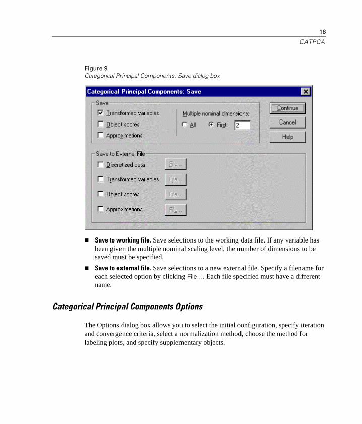
Categorical Principal Components Save

The Save dialog box allows you to add the transformed variables, object scores, and approximations to the working data file or as new variables in external files and save the discretized data as new variables in an external data file.

16

CATPCA

Figure 9Categorical Principal Components: Save dialog box

n Save to working file. Save selections to the working data file. If any variable has been given the multiple nominal scaling level, the number of dimensions to be saved must be specified.

n Save to external file. Save selections to a new external file. Specify a filename for each selected option by clicking File…. Each file specified must have a different name.

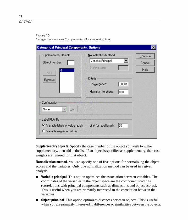
Categorical Principal Components Options

The Options dialog box allows you to select the initial configuration, specify iteration and convergence criteria, select a normalization method, choose the method for labeling plots, and specify supplementary objects.

17

CATPCA

Figure 10Categorical Principal Components: Options dialog box

Supplementary objects. Specify the case number of the object you wish to make supplementary, then add to the list. If an object is specified as supplementary, then case weights are ignored for that object.

Normalization method. You can specify one of five options for normalizing the object scores and the variables. Only one normalization method can be used in a given analysis.

n Variable principal. This option optimizes the association between variables. The coordinates of the variables in the object space are the component loadings (correlations with principal components such as dimensions and object scores). This is useful when you are primarily interested in the correlation between the variables.

n Object principal. This option optimizes distances between objects. This is useful when you are primarily interested in differences or similarities between the objects.

18

CATPCA

n Symmetrical. Use this normalization option if you are primarily interested in the relation between objects and variables.

n Independent. Use this normalization option if you want to examine distances between objects and correlations between variables separately.

n Custom. You can specify any real value in the closed interval [-1, 1]. A value of 1 is equal to the Object Principal method, a value of 0 is equal to the Symmetrical method, and a value of -1 is equal to the Variable Principal method. By specifying a value greater than -1 and less than 1, you can spread the eigenvalue over both objects and variables. This method is useful for making a tailor-made biplot or triplot.

Criteria. You can specify the maximum number of iterations the procedure can go through in its computations. You can also select a convergence criterion value. The algorithm stops iterating if the difference in total fit between the last two iterations is less than the convergence value or if the maximum number of iterations is reached.

Configuration. You can read data from a file containing the coordinates of a configuration. The first variable in the file should contain the coordinates for the first dimension, the second variable should contain the coordinates for the second dimension, and so forth.

n Initial. The configuration in the file specified will be used as the starting point of the analysis.

n Fixed. The configuration in the file specified will be used to fit in the variables. The variables that are fitted in must be selected as analysis variables, but because the configuration is fixed, they are treated as supplementary variables (so they do not need to be selected as supplementary variables).

Label plots by. Allows you to specify whether variables and value labels or variable names and values will be used in the plots. You can also specify a maximum length for labels.

CATPCA Command Additional Features

You can customize your categorical principal components analysis if you paste your selections into a syntax window and edit the resulting CATPCA command syntax. SPSS command language also allows you to:

19

CATPCA

n Specify rootnames for the transformed variables, object scores, and approximations when saving them to the working data file (with the SAVE subcommand).

n Specify a maximum length for labels for each plot separately (with the PLOT subcommand).

n Specify a separate variable list for residual plots (with the PLOT subcommand).