Catchment-based gold prospectivity analysis combininggeochemical, geophysical and geological data acrossnorthern Australia

M. J. Cracknell1* & P. de Caritat2,31 CODES Centre of Excellence in Ore Deposits, University of Tasmania, Hobart TAS 7001, Australia2 Geoscience Australia, GPO Box 378, Canberra ACT 2601, Australia3 Research School of Earth Sciences, The Australian National University, Canberra ACT 2601, Australia

M.J.C., 0000-0001-9843-8251; P.d.C., 0000-0002-4185-9124*Correspondence: m.j.cracknell@utas.edu.au

Abstract: The results of a pilot study into the application of an unsupervised clustering approach to the analysis of catchment-based National Geochemical Survey of Australia (NGSA) geochemical data combined with geophysical and geological dataacross northern Australia are documented. NGSAMobileMetal Ion® (MMI) element concentrations and first and second orderstatistical summaries across catchments of geophysical data and geological data are integrated and analysed usingSelf-OrganizingMaps (SOM). Input features that contribute significantly to the separation of catchment clusters are objectivelyidentified and assessed.

A case study of the application of SOM for assessing the spatial relationships between Au mines and mineral occurrences incatchment clusters is presented. Catchments with high mean Au code-vector concentrations are found downstream of areasknown to host Au mineralization. This knowledge is used to identify upstream catchments exhibiting geophysical andgeological features that indicate likely Au mineralization. The approach documented here suggests that catchment-basedgeochemical data and summaries of geophysical and geological data can be combined to highlight areas that potentially hostpreviously unrecognised Au mineralization.

Keywords: Regolith; Geochemistry; Geophysics; Geology; Self-Organizing Maps; National Geochemical Survey ofAustralia

Received 10 October 2016; revised 7 March 2017; accepted 8 March 2017

Regolith cover

Unweathered rock outcrop is rare across the Australian continentwith more than 85% of its surface being covered by regolith(Wilford 2012). Although the majority of the continent is classifiedas having an arid to semi-arid climate, the wide range of regolithtypes found across Australia is a result of contrasting parentmaterials, long-term landscape evolution, diverse vegetationcommunities, and (palaeo-)climate extremes (Taylor & Butt1998; Mann et al. 2012; Pain et al. 2012). The ubiquity of theregolith and its highly diverse characteristics present significantchallenges to developing a clear understanding of the nature of thesesurface materials. In light of this challenge, a key theme of theUNCOVER initiative is to characterise regolith geochemical andgeophysical properties (UNCOVER 2012). Information on regolithproperties and formative (consistent with L1334) processes iscrucial for developing new mineral exploration models in areaswhere prospective bedrock is concealed by surface material.

The National Geochemical Survey of Australia

Recently, Geoscience Australia with its State/NT partnersembarked on a systematic continental-scale geochemical samplingprogram, the National Geochemical Survey of Australia (NGSA;Caritat & Cooper 2011a). The aim of the NGSA project was toprovide ultra-low (spatial) density compositional data and infor-mation regarding the near-surface regolith to advance explorationfor energy and mineral resources. The results of NGSA analyses arebeing used to improve our understanding of the concentration

levels, spatial distribution, associations and their genesis andsignificance, transport processes, and sources and sinks ofgeochemical elements in the near-surface environment (e.g. seeCaritat & Cooper 2016).

One of the key challenges to analysing the NGSA dataset is that itcontains a large number of variables or features collected acrossnearly all the geological and biological regions of Australia. Recentresearch has explored the use of robust multivariate statisticalanalysis to identify and understand the distribution of geochemicalelements analysed in the NGSA data (e.g. Caritat & Grunsky 2013;Scealy et al. 2015). Caritat & Cooper (2016) provide an up-to-datesummary of studies using NGSA data for investigating geochemicalprocesses for mineral exploration, agriculture and understandingcontamination sources at continental and regional scales. Some ofthe studies that specifically relate to mineral exploration and employmethods for multivariate analysis are briefly summarized below ascontext to the present work.

Caritat et al. (2011) identified geochemical patterns in theMobileMetal Ions® (MMI) analyses related to the spatial distribution ofgeneralised lithological types by comparing geochemical patterns inthe NGSA data to surface geology polygons. For example, samplestaken from within the Great Artesian Basin and Murray-DarlingBasin sedimentary provinces were found to exhibit elevated Ba, Gaand Sr concentrations. Conversely, elevated La, Ce and other rareearth elements (REEs) were found to be spatially coincident withareas where felsic intrusive rocks dominate, such as easternAustralia and SW Western Australia (WA). High-grade meta-morphic terrains were spatially correlated with moderate concentra-tions of MMI Cs, K, Mo, Rb and W.

© 2017 Commonwealth of Australia (Geoscience Australia). This is an Open Access article distributed under the terms of the Creative CommonsAttribution License (http://creativecommons.org/licenses/by/3.0/). Published by The Geological Society of London for GSL and AAG. Publishing disclaimer:www.geolsoc.org.uk/pub_ethics

Thematic set article: Analysis of Exploration Geochemical Data Geochemistry: Exploration, Environment, Analysis

Published online June 1, 2017 https://doi.org/10.1144/geochem2016-012 | Vol. 17 | 2017 | pp. 204–216

by guest on July 15, 2018http://geea.lyellcollection.org/Downloaded from

Mann et al. (2013) analysed the relationship between mineraldeposits and MMI element concentrations by identifying catch-ments with elevated commodity element concentrations and alsocontaining mineral deposits. They found a reasonable spatialcorrelation with elevated Au concentrations and provinces knownto host major Au mineralization. This observation was used tosuggest that elevated Au concentrations in areas that do notcontain known Au mineralization potentially form a usefulexploration lead into areas such as the western Albany-Fraserbelt in WA.

Caritat & Grunsky (2013) used principal component analysis tosummarize and interpret NGSA geochemical data (total concentra-tions). They found that the first four principal components (PCs)accounted for 59% of the variance in the dataset. The elementassociations represented by these PCs relate to geological processessuch as lithological controls, weathering, transport and secondarymineral precipitation. Based on these findings, Caritat & Grunsky(2013) identified lithological prediction (e.g. Grunsky et al. 2017)and mineral prospectivity analysis (e.g. this study) as potential usesof the NGSA dataset.

Spatial support

The interpolation of NGSA point data, which represent the overallsediment geochemical characteristics of catchments, into 2D mapsvia linear kriging of for instance the top ranked PCs generatescontinuously varying surfaces (rasters). The resulting surfaces donot conform to the discretised areal summary (watersheds orcatchments) of geochemical characteristics that the NGSA datarepresent. While this may be a valid approach for defining broadcontinental-scale spatial trends in geochemical concentrations, itassumes a different spatial support, e.g. point locations, to thatrepresented by catchment outlet sediments, which are transportedsediments derived from upstream sources. Thus, NGSA dataprovide a representative indication of the overall geochemicalcharacteristics of rocks and soils within a catchment (Caritat &Cooper 2011a) and potentially a catchment’s entire upstreamwatershed.

In this study, we use an approach that does not assume theprocesses under consideration to be continuously varying ingeographic space, that is, we generate spatial models using amultivariate statistical approach that not only preserves thecatchment-based spatial support but also maintains the directcontribution of input features to quantifying the similarities anddissimilarities between catchments. Furthermore, we integrategeophysical and geological data, widely available across theAustralian continent, with geochemical analyses to provide adeeper understanding of bedrock and regolith characteristics withinNGSA catchments across much of northern Australia. This is to ourknowledge only the second time such an approach has been appliedto interrogating cross-disciplinary datasets with the aim ofelucidating geological processes (see below).

Self-Organizing Maps

Self-Organizing Maps (SOM; Kohonen 1982, 2001) is anunsupervised clustering method useful for finding natural groupswithin complex multivariate data. SOM aids visualization andinterpretation by reducing n-dimensional (nD) multivariate data to atwo-dimensional ‘map’ where the spatial arrangement of neigh-bouring groups is representative of their similarities in nD space(Penn 2005; Bierlein et al. 2008). SOMuses vector quantization andmeasures of vector similarity, typically Euclidean distances, as ameans of grouping input samples. The resultant groups or nodes arerepresented by a vector (code-vector) that summarises the propertiesof the associated input samples. Visualization of SOM component

planes assists the interpretation of patterns and structures within theinput data (Penn 2005; Bierlein et al. 2008; Löhr et al. 2010). Formore detailed descriptions of SOM implementation and theory seeSun et al. (2009) and Cracknell et al. (2015).

Unlike other statistical clustering methods, such as factoranalysis or k-means, SOM does not assume Gaussian distributions(Löhr et al. 2010; Žibret & Šajn, 2010). This is an importantconsideration for the analysis of geochemical data as these data arerarely normally or even log-normally distributed (Reimann &Filzmoser 2000). Previous research demonstrating the applicationof SOM for the analysis of geological and environmental patterns ingeochemical data include Lacassie et al. (2004), Lacassie & RuizDel Solar (2006), Tsakovski et al. (2009), Sun et al. (2009), Löhret al. (2010) and Žibret & Šajn (2010). In contrast to the researchcited above that only analysed geochemical data, Cracknell et al.(2014) used SOM to combine interpolated soil geochemical andgeophysical data. The resulting SOM clusters identified spatiallyconsistent domains representing subtle geochemical contrastsrelated to changes in primary magmatic composition andhydrothermal alteration.

Study area

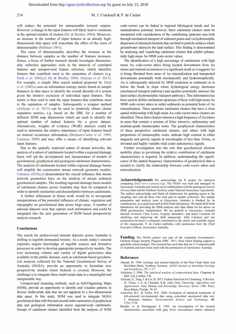
The study region covers c. 1.3 million km2 across the NorthernTerritory and western Queensland in northern Australia (Fig. 1).This area was chosen primarily for the development of analysismethods documented in this pilot study as it is large enough to covera substantial number of NGSA catchments but small enough torapidly generate results. Furthermore, the study area contains arange of mineralization styles and includes geological materialsfrom a wide variety of ages ranging from Proterozoic to Cenozoic(including Quaternary sediments; Fig. 2) and lithological types(Fig. 3). Finally, northern Australia is currently the subject ofattention and investment (e.g. the 2016 – 2020 ‘Exploring for theFuture’ Programme of the Australian Government) and is thus botha topical and timely focus for the demonstration of the cross-disciplinary SOM approach developed here.

The oldest rocks in the study area are Palaeoproterozoic toMesoproterozoic in age and are found in the Arunta, Tanami,Davenport, Tennant Creek, Isa, McArthur and Georgetowngeological regions (see Fig. 2). Their dominant rock types aregranulite facies metamorphosed felsic and mafic volcanics, finegrained clastic and carbonate metasediments, amphibolite faciesturbidites and carbonaceous metasediments, folded greywackes andsiltstones, clastic sedimentary rocks and metamorphosed volcanicrocks intruded by mafic and felsic (Blake et al. 1987; Ferenczi &Ahmad 1998; Wygralak & Bajwah 1998). The economicallysignificant Isa and McArthur geological regions, as well as theGeorgetown geological region, are hosts to a range of mineralizationand deposit types, e.g. Au, base metals, Sn, W and Ta (Blake et al.1987; Ahmad 1998; Ferenczi & Ahmad 1998; Wygralak & Bajwah1998; Budd 2001; Withnall & Hutton 2013). The main Palaeozoicgeological regions in the study area are the Georgina and Wisogeological regions (see Fig. 2). Their dominant rock types are clasticand carbonate sedimentary rocks, and regolith (Smith 1972; Kruse& Munson 2013). Known resources include phosphate and U, aswell as groundwater, oil and gas (Smart et al. 1972; Radke 2009;Kruse & Munson 2013).

Aims

This study integrates catchment-based MMI geochemical data withgeophysical imagery and geological information using SOM withthe aim of objectively identifying groups of catchments with similargeochemical, geophysical and geological properties. Once identi-fied, these catchment clusters are visually analysed in both data

205Catchment-based gold prospectivity

by guest on July 15, 2018http://geea.lyellcollection.org/Downloaded from

space and geographic space. The integrated interrogation ofcatchment clusters –with respect to other geoscience data, includinglithology, mineral deposits and mineral occurrences – are then usedto formulate a Au mineral exploration model.

Materials and methods

All data used are publicly available from Geoscience Australia andwere transformed to the Lambert Conformal Conical (GeoscienceAustralia) projection prior to analysis.

Geochemical data

Catchment-based geochemical data were sourced from the NGSA(Caritat & Cooper 2011a). A total of 225 NGSA catchments, c. 1/6of the total number of NGSA catchments, were selected for thepresent SOM analysis. Analysis was performed on bulk properties(e.g. pH, electrical conductivity) and theMMI geochemical elementassay data, the latter being determined on the coarse fraction(<2 mm) of top outlet sediment (TOS) samples (0 – 10 cm depth). Acomprehensive quality assessment of the NGSA data describing

Fig. 2. Generalised geological regions (Blake & Kilgour 1998) across the study area, colour coded by age. For interpretation of the references to colour inthis figure, the reader is referred to the online version of this article.

Fig. 1. Map of Australia showing selectedNational Geochemical Survey of Australia(NGSA; Caritat & Cooper 2011a) samplelocations (red points) and the 225catchments selected for this study (greypolygons) overlain with the Australianriver network (blue polylines)(Geoscience Australia 2003). Forinterpretation of the references to colour inthis figure, the reader is referred to theonline version of this article.

206 M. J. Cracknell & P. de Caritat

by guest on July 15, 2018http://geea.lyellcollection.org/Downloaded from

precision, bias, and censoring proportion is in the public domain(Caritat & Cooper 2011b). The scope of the present study waslimited to the MMI data because this method extracts looselyadsorbed ions from the surfaces of minerals, organic matter andFe-oxyhydroxides; thus, MMI results can be indicative of elementsthat have moved relatively recently through the regolith, which canreflect unusual element concentrations at depth potentiallyindicative of lithology or mineralization (Mann 2010).Consequently, these data are well suited to potentially identifyingburied mineral deposits.

Bulk sediment properties data used included pH, electricalconductivity (EC), and percent fractions of clay, silt and sand. ECvalues were log transformed to approximate a normal distribution asthese data are typically log-normally distributed (McKenzie et al.2008). One catchment within the study area was excluded fromanalysis due to missing bulk properties data.

MMI element data that contained half or more samples withcensored results (below the detection limit) were excluded fromanalysis. For the remaining 42 elements (Ag, Al, Au, Ba, Ca, Cd,Ce, Co, Cr, Cs, Cu, Dy, Er, Eu, Fe, Ga, Gd, K, La, Li, Mg, Mn, Mo,Nd, Ni, P, Pb, Pr, Rb, Sc, Se, Sm, Sr, Tb, Th, Ti, U, V, Y, Yb, Zn andZr), censored values were replaced by half the appropriate detectionlimit, a common practice in geochemistry (e.g. Botnick & White

1998; Helsel 2005; Antweiler & Taylor 2008; Carranza 2011). Thedata were then centred log-ratio (clr) transformed as described byAitchison (1986) and in-line with other studies investigating thespatial variability of NGSA geochemical data (e.g. Caritat &Grunsky 2013; Mueller et al. 2014; Furman et al. 2016).

Geophysical data

The latest versions of total magnetic intensity (MAG; Percival2014) with variable reduction-to-pole corrections applied (Version6), filtered total count (dose) radiometrics Version 3 (TC; Mintyet al. 2009) and spherical cap Bouguer gravity anomaly (GRAV;Tracey et al. 2007) raster data were clipped to the study area extentand resampled from their original resolutions to a 1000 m cellresolution using bilinear interpolation. Geophysical data resamplingwas carried out to avoid memory usage errors when processing thegrey level co-occurrence matrix (GLCM; see below) textures and toenhance regional-scale geological features.

From the cells intersecting a given catchment, first order spatialstatistics (mean and standard deviation) and second order spatialstatistics (e.g. GLCM) for each geophysical input were calculated.The resulting first and second order spatial statistics were appendedto the geochemical data acquired from each catchment. First order

Fig. 3. Generalised lithologies (Raymond & Gallagher 2012) across the study area, colour coded by type. For interpretation of the references to colour inthis figure, the reader is referred to the online version of this article.

Table 1. Quantization and topological errors for 10 different combinations of X and Y dimensions with c. 200 node

X dim Y dim Nodes Quantization error Topological error

* 6 33 198 1.13 7.498 25 200 1.14 7.8110 20 200 1.13 8.0012 17 204 1.13 8.2014 14 196 1.15 8.4816 12 192 1.14 8.2818 11 198 1.14 8.2020 10 200 1.14 7.9622 9 198 1.14 7.9324 8 192 1.14 8.00

Optimal SOM map dimensions (6 by 33) indicated by *.

207Catchment-based gold prospectivity

by guest on July 15, 2018http://geea.lyellcollection.org/Downloaded from

spatial statistics were obtained by summarizing all cell values acrossa given catchment. Second order spatial statistics (texture) wereobtained by assessing the spatial variability of all cell values at aparticular scale (offset) within a given neighbourhood (Gonzalez &Woods 2008) usingGLCM (Haralick et al. 1973). ThemeanGLCMcontrast index averaged across the four principal directions (north–south, NE–SW, east–west and SE–NW) was used to representspatial texture across a given catchment for 10 offsets withincrements of c. 2 km (i.e. 2, 4, …, 20 km).

GLCM contrast is defined as (Baraldi & Parmiggiani 1995):

GLCMcon ¼XNg�1

i¼0

XNg�1

j¼0

(i� j)2g(i, j)

where Ng is the number of grey levels in an image, i and j representthe ith and jth grey levels respectively and g(i, j) is defined as the(i, j)th entry in the GLCM such that:

g(i, j) ¼ p(i, j)PNg�1

i¼0

PNg�1j¼0 p(i, j)

where p(i,j) is the occurrence of unique pairwise combinations ofgrey levels i and jmeasured at two pixels separated by a given offset.GLCM contrast is correlated with spatial frequencies such that ahigh value of GLCMcon for a given offset and measured valueindicates a large relative difference at that offset distance (Baraldi &Parmiggiani 1995).

Ancillary data

The OZMIN database (Ewers et al. 2002) of mines and mineraldeposits and occurrences was used to assess the type and frequencyof mineral occurrences within individual catchment clusters. Terrainslope was derived from GEODATA 9 second (c. 250 m resolution)digital elevation model (DEM) version 3 (Geoscience Australia2008) using the slope function in QGIS version 2.12.1. The1:2 500 000 scale Surface Geology of Australia (Raymond &Gallagher 2012) was used to summarize the dominant generalizedlithological units intersecting a given catchment cluster.

SOM implementation

A total of 83 input variables representing geochemical, geophysicaland geological properties were range normalised to 0–1 using alinear transformation. SOMwas implemented using the R statisticalprogramming language package som (Yan 2010), which is based onSOM-PAK (Kohonen et al. 1996). Multiple trials of different X andY SOM map dimensions for c. 200 randomly seeded nodes withhexagonal topologies were initiated and run for over 10 000iterations with a Gaussian neighbourhood function and inverselearning function (Kohonen et al. 1996). Optimal SOM mapdimensions were identified by minimizing quantization andtopological errors. For more information on the theory andderivation of SOM quantization and topological errors used heresee Cracknell et al. (2015).

Cluster selection and properties

Once an optimal SOM model was selected for c. 200 nodes, ahierarchical dendrogram agglomerative clustering method wasemployed to merge SOM nodes based on their code-vectors(Vesanto & Alhoniemi 2000; Cracknell et al. 2015). The Davies-Bouldin Index (DBI; Davies & Bouldin 1979), which estimatescluster similarity using the maximum mean ratio of clusterdispersion and pairwise centroid distances, was used to identifyan optimal number of clusters (i.e. merged SOM nodes).

Input variables that contributed significantly high or low SOMcode-vector values, with respect to other cluster code-vector values,were identified using the following formula, modified fromSiponen et al. (2001):

ri ¼ s(i, k)1

c� 1

Xj=i

s(j, k)� 1

where s(i,k) is the mean cluster i code-vector for input variable k ands( j,k) is the mean cluster j code-vector for input variable k. Thisratio provides an indication of the relative difference of k in cluster ias compared to the mean code-vector values of all other clusters j(Siponen et al. 2001). For example, values >>0 indicate clusterswith substantially higher mean code-vector values compared to themean values of all other clusters. Conversely, values <<0 indicateclusters with substantially lower mean code-vector values comparedto the mean values of all other clusters. Variables contributingsignificantly higher (or lower) values to a given cluster are identifiedas those with code-vector ratios greater (or lower) than one standarddeviation from the mean code-vector ratio.

Results

A 6 by 33 (X by Y) SOMmap with 198 nodes was found to result inthe minimum mean quantization and topological errors (Table 1).The DBI as a function of merged SOM nodes (up to 25 mergednodes) identified 19 as the optimal minimum number of clusters(Fig. 4), although other local minimum DBI values were observedfor 4 and 8 clusters. A plot of the spatial distribution of resultingcatchment clusters is shown in Figure 5.

The relative positions of catchment clusters on the Au componentplane plot are presented in Figure 6a. The catchment clusters withsignificantly high mean Au code-vector ratios (warm colours) plottogether near the top of the SOM map (refer to the online version ofthis article). Figure 6b plots cluster mean code-vector ratios of Auconcentration as compared to all other clusters. Clusters 15, 14, 17, 16and 12 are identified as exhibiting mean Au code-vector ratios greaterthan one standard deviation above the mean Au code-vector ratio.

Figure 7a maps the locations of clusters identified in Figure 6bthat display mean Au code-vector ratios greater than one standarddeviation above the mean (bold outlines), as well as the clrtransformed values of MMI Au concentrations (colour scale),overlain with Au mines and mineral occurrences (red stars).Figure 7b plots catchment clusters with high Au mean code-vectoroverlain with terrain slope as greyscale pixels. At first glance theredoes not appear to be any spatial relationship between Aumines andhigh catchment Au concentrations or catchment clusters with highmean Au code-vector ratios, however, catchments with high meanAu code-vector ratios are positioned at the transition from relativelyhigh slope to low slope (i.e. break in slope) downstream from Aumine and mineral occurrence locations. Visual comparison ofcatchment clusters 15, 14, 17, 16 or 12 indicates that 41 out of these

Fig. 4. Davies-Bouldin Index (DBI: Davies & Bouldin 1979) as a functionof the number of merged SOM nodes for the 6 by 33 SOM model.

208 M. J. Cracknell & P. de Caritat

by guest on July 15, 2018http://geea.lyellcollection.org/Downloaded from

54 catchments (76%) have a portion of their extent intersecting abreak in slope.

Figure 8 shows catchments with high mean Au code-vectors(clusters 15, 14, 17, 16 or 12) and upstream catchment clusters 4,

6 and 9 identified by visually interrogating mapped relationships.Catchment clusters 4, 6 and 9 were selected by manually queryingregions upstream of catchment clusters 15, 14, 17, 16 and 12 andtaking note of regularly occurring cluster indices. These upstream

Fig. 5. Spatial distribution of the 19 catchment clusters for SOM map dimensions 6 by 33 and 198 nodes. For interpretation of the references to colour inthis figure, the reader is referred to the online version of this article.

Fig. 6. (a) 2D SOM map and Au component plane with division of final catchment clusters and (b) mean code-vector ratios for cluster Au concentration.Five clusters display higher that one standard deviation from the mean (dashed line) code-vector ratio. For interpretation of the references to colour in thisfigure, the reader is referred to the online version of this article.

209Catchment-based gold prospectivity

by guest on July 15, 2018http://geea.lyellcollection.org/Downloaded from

catchment clusters are found to have a close spatial associationwith catchments hosting Au mines and mineral occurrences andplot as immediate neighbours to each other on the SOM 2D map(Fig. 6a). By combining stream network information the proportionof catchments containing Au mines that are directly upstream of oneor more NGSA catchment clusters 15, 14, 17, 16 or 12 wascalculated. Of the 31 NGSA catchments in the study area thatcontain Au mineralization, 28 have flow paths that are not internallydraining, i.e. we have omitted three catchments (located in thesouthern region of the Northern Territory) with confused flow paths.Of these 28 catchments (13% of the total number of catchments), 21are linked downstream to NGSA catchment clusters with high meanAu code-vector (24% of the total number of catchments). Thisindicates that 75% of the catchments with Au mineralization areupstream of NGSA catchment clusters 15, 14, 17, 16 or 12. Ifcatchment clusters 4, 6 and 9 (a further 18% of the total number ofcatchments) are included, 27 (96%) of the 28 Au mineralisedcatchments are upstream of catchment clusters identified in thisstudy. In contrast, of the 63 catchments (28% of the total number of

catchments) within the study area that display high Au concentra-tions (i.e. Au clr values between −2.00 to −1.50 and −1.50 to−1.29, see Fig. 7a) only 10 (16%) are located downstream ofcatchments with known Au mines and mineral occurrences.

Table 2 summarizes the significantly high and low code-vectorvalues for all catchment clusters with the frequency of mines andmineral occurrences for a given (dominant) commodity thatintersects these clusters. The upstream catchment clusters 4 and 6are characterized by low concentrations in fine clastic components(i.e. clay and silt). Cluster 4 displays high contrast in magnetics fordistances less than 10 km and low contrast in magnetics for greaterthan 10 km. Cluster 9 exhibits a high contrast in gravity forwavelengths less than 10 km and low contrast for wavelengths of12 – 14 km. All upstream catchment clusters (4, 6 and 9) contain ahigh frequency of Au mines and mineral occurrences with cluster 4also containing many Agmines, cluster 6 Cumines and cluster 9 Cuand U mines.

Table 3 ranks generalized lithological units within clusters 4, 6and 9 based on differences in the proportion of area for a given unit

Fig. 7. (a) Spatial distribution of clusters with mean Au concentration code-vector ratios greater than one standard deviation from the mean, and Au minesand mineral occurrences locations overlain on colour coded NGSA catchment centred log-ratio transformed Au concentration. (b) NGSA catchment clusterswith high Au mean code-vectors overlain on terrain slope. Note that clusters with high Au code-vector ratios are found immediately downstream of most Aumines at the break in slope. For interpretation of the references to colour in this figure, the reader is referred to the online version of this article.

210 M. J. Cracknell & P. de Caritat

by guest on July 15, 2018http://geea.lyellcollection.org/Downloaded from

compared to their overall proportion across the entire study area.Hence, positive values highlight lithological units that cover a largerproportion of the cluster area with respect to the mean of allcatchments. Clusters 4 and 9 contain large proportions of felsicintrusive rocks and low proportions of surficial or regolith units.Clusters 4 and 6 contain high proportions of medium-gradedmetamorphic rocks, while clusters 6 and 9 show high proportions ofsedimentary rocks and low proportions of high-grade metamorphicrocks.

Discussion

Present work

NGSA samples were collected as catchment outlet (overbank orfloodplain) sediments. Overbank sediments have been shown to bemore representative of the geochemical composition of thecatchment than stream sediments (Ottesen et al. 1989). This isbecause the suspended sediment load in a flood event, from whichthe overbank or floodplain sediments are primarily derived, issourced from a greater area than the sediments within the streamchannel, which are typically derived from local point sources. Thus,catchment outlet sediments are assumed to represent an integratedsample of the entire catchment area (Ottesen et al. 1989; Bølvikenet al. 2004). Furthermore, outlet sediments are ubiquitous across adiverse range of geomorphological and climatological regions. Theresults presented in this study indicate that the geochemicalcharacteristics of outlet sediments sampled from large riversystems are likely to be representative of both the immediatecatchment watershed and the upstream drainage basin from whichthese sediments are potentially derived.

TheMMI extraction, however, was developed to mainly mobilisethe labile fraction of chemical elements, presumably from the outersurfaces of soil particles (Mann 2010). Accordingly the MMIresponse can be subdued after significant rain and flooding, but canalso reform relatively quickly (Mann et al. 2005). Thus the system

investigated geochemically here is a fairly dynamic one, especiallyin the region of interest where rainfall is seasonal (typical dry andwet seasons in winter and summer respectively). The reasonwhy theMMI geochemical characteristics of outlet sediments sampled fromlarge river systems are likely to be representative of both theimmediate catchment watershed and the upstream drainage basin isthrough a combination of mechanical transport of sediment grainsand hydromorphic dispersion of geochemical signatures throughgroundwater flow systems. Whilst the sediment matrix is physicallyinherited from both the catchment where the outlet sediment issampled and potentially that upstream, the surface adsorbed, labilechemical (MMI) signature may form as groundwater rises to thesurface at topographic breaks in slope. If groundwater is in direct orindirect contact with mineralised basement in the upstream (part ofa) catchment it can acquire and transport downstream a geochemicalsignature diagnostic of this (e.g. Leybourne & Cameron 2010). Inthe case of Au, the MMI response in sediments likely arises from acombination of the etching of clastic gold grains (placer pathway)and the extraction of labile, adsorbed fine secondary Au on particlesurfaces (hydromorphic pathway) (A. Mann, pers. comm. 2017).

The information in Table 2 summarizes catchment clustercharacteristics that contribute significantly to their dissimilarities(or similarities) to other clusters. This information provides atentative indication of the lithological origins of the outlet sedimentsanalysed. For example, clusters 1, 2, and 4 have high Ce, La andREEs suggesting felsic igneous dominant sources (Caritat et al.2011), while also exhibiting a high total count first order mean.Clusters 1, 3 and 4 display high sand content, high Th and Zr.Clusters 1 to 4 display significantly low pH, EC, Au, Cu, Ca, Ba,Co, Mg, Ni and Sr. Many of these elements are typically associatedwith mafic igneous lithological sources. These observations suggestfelsic igneous sources for clusters 1–4. Clusters 1 and 3 display lowcontrast in gravity at wavelengths of less than or equal to 10 km andclusters 2 and 4 display low contrast in magnetism at wavelengthsgreater than 10 km. The geophysical characteristics of these clusterspotentially provide an indication of the maximum ‘size’ of felsic

Fig. 8. Spatial distribution of catchments with high Au concentration (colour intensity indicates Au concentration rank, see Fig. 6) and neighbouringupstream catchment clusters 4, 6 and 9. For interpretation of the references to colour in this figure, the reader is referred to the online version of this article.

211Catchment-based gold prospectivity

by guest on July 15, 2018http://geea.lyellcollection.org/Downloaded from

igneous features, e.g. low gravity contrasts within plutons and highmagnetic ‘alteration’ in contact zones. Furthermore, the majority ofclusters 1–4 either intersect Proterozoic geological regions such as

the Arunta, Isa or Georgetown regions, or are immediatelydownstream of one, e.g. north and NE of the Tennant Creek, andeast of the South Nicholson geological regions. These clusters also

Table 2. Summary of upstream catchment cluster high and low code-vector values and the frequency of intersecting mines and mineral occurrences based on theOZMIN database (Ewers et al. 2002) for a given mineral commodity

High code to vector ratio Low code to vector ratio Commodity (frequency)

Cluster 1 Sand, Ce, Cs, Eu, Fe, Gd, La, Nd, Pr, Rb,Sc, Sm, Tb, Th, Ti, ZrTC-mean, TC-14con to TC-20con,GRAV-std, GRAV-12con toGRAV-20con

pH, EC, Silt, Clay, Ag, Au, Ba, Ca, Cd, Co, Cu,Ga, K, Li, Mg, Mo, Ni, SrMAG-mean, TC-8con to TC-10con,GRAV-2con to GRAV-10con

U3O8 (4), Fe (1)

Cluster 2 Ce, Cr, Cs, Dy, Er, Eu, Fe, Gd, La, Nd, Pb,Pr, Sc, Sm, Tb, Th, Ti, Y, Yb, ZrMAG-2con to MAG-8con, TC-mean,TC-std

pH, EC, Clay, Al, Au, Ba, Ca, Cd, Co, Cu, Ga,K, Li, Mg, Mn, Mo, Ni, Sr, U, ZnMAG-mean, MAG-std, MAG-12con toMAG-18con

Au (1), U3O8 (1)

Cluster 3 Sand, Eu, La, Nd, P, Pr, Rb, Sc, Th, ZrGRAV-std, GRAV-12con to GRAV-18con

pH, EC, Silt, Clay, Ag, Au, Ba, Ca, Co, Cu, Ga,Mg, Ni, Pb, SrMAG-mean, MAG-8con to MAG-10con,TC-2con to TC-10con, GRAV-6con toGRAV-10con

P2O5 (3), Mo (1)

Cluster 4 Sand, Ce, Cr, Cs, Dy, Eu, Fe, Gd, La, Nd,Pr, Sc, Sm, Tb, Th, Ti, ZrMAG-2con to MAG-10con, TC-mean,TC-std

pH, EC, Silt, Clay, Al, Au, Ba, Ca, Cd, Co, Cu,Ga, K, Mg, Mn, Ni, Sr, VMAG-12con to MAG-20con

Ag (5), Au (4) Co (1), Cu (1), P2O5 (1)

Cluster 5 Sand, P, Rb Silt, Clay, Co, Pb Au (2), Ag (1)Cluster 6 Nd, Zn

MAG-10conClay, Co, Cs, Pb, Se, VTC-mean

Au (5), Cu (3), Mn (1), P2O5 (1), U3O8 (1)

Cluster 7 TC-2con to TC-6con Cr, Cs, PbMAG-std, TC-18con to TC-20con

Au (2), Cu (1)

Cluster 8 MnMAG-12con to MAG-20con,TC-2con to TC-10con

Cr, Cs, Rb, UMAG-std, MAG-2con to MAG-10con,TC-12con to TC-16con

P2O5 (4), Ag (1), Fe (1), Pb (1)

Cluster 9 Dy, Er, Gd, Tb, Y, YbTC-4con to TC-10con, GRAV-2con toGRAV-10con

Cr, Cs, Mo, Rb, Se to Ti, VGRAV-12con to GRAV-14con

Au (4), Cu (7), Fe (1), P2O5 (1), U3O8 (4)

Cluster 10 MAG-mean, MAG-std, MAG-8con toMAG-10con, GRAV-mean,GRAV-2con to GRAV-10con

Fe, Rb, ZnGRAV-12con to GRAV-20con

Cu (20), U3O8 (7), Au (12), Co (3), Fe (3),Mn (3), Ag (2), P2O5 (2), Pb (1)

Cluster 11 MAG-12con to MAG-20con, TC-2con toTC-10con

Rb, UMAG-2con to MAG-4con, TC-std,TC-12con, GRAV-std

Ag (1), Dmd (1)

Cluster 12 Silt, Clay, Ag, Au, Co, Ga, PbTC-2con to TC-10con, GRAV-10con

Sand, La, P, Pr, ZrTC-mean, TC-std, TC-12con to TC-16con

Au (10), Cu (1), Mn (1), Y2O3 (1)

Cluster 13 MAG-mean, MAG-std, MAG-4con toMAG-10con, GRAV-2con to GRAV-10con

Fe, P, TiMAG-12con to MAG-16con, GRAV-12conto GRAV-20con

Cu (6), Au (4), REO (1)

Cluster 14 pH, Silt, Clay, Ag, Al, Au, Cd, Co, Cu, Li,Mo, Pb, Se, Sr, U, V, YbMAG-2con to MAG-10con

Sand, Ce, Eu, Fe, La, Nd, P, Pr, Sm, Th, Ti,ZrMAG-12con to MAG-20con

Au (3), Ag (2),Cu (2), P2O5 (2),Mo (1), U3O8 (1), WO3 (1), Zn (1)

Cluster 15 pH, EC, Silt, Clay, Ag, Au, Ba, Cd, Co,Cu, Ga, Li, Mg, Mo, Pb, Sr, V

Sand, Ce, Dy, Eu, Gd, La, Nd, P, Pr, Sm, Tb,Th, Y, ZrTC-mean, TC-std

P2O5 (2), Cu (1)

Cluster 16 pH, EC, Clay, Au, Ca, Cd, Cu, K, Li, Mg,Mo, Rb, Se, Sr, U, V, Zn

Ce, Dy, Eu, Fe, Gd, La, Nd, Pr, Sm, Tb, Th,YMAG-20con

P2O5 (5), Ag (3), Au (2),Pb (1), U3O8 (1), Zn (1)

Cluster 17 pH, Clay, Ag, Al, Au, Ba, Ca, Cd, Cu, Ga,K, Li, Mg, Mn, Mo, Ni, Sr, U, V, ZnMAG-12con toMAG-20con, TC-16conto TC-18con to TC-20con, GRAV-20con

Ce, Dy, Er, Eu, Gd, La, Nd, Pr, Sm, Tb, Th, Y,YbMAG-2con to MAG-10con, TC-mean,TC-2con, GRAV-mean

–

Cluster 18 EC, K, UTC-mean, TC-std, TC-12con to TC-20con, GRAV-std, GRAV-12con toGRAV-20con

TC-2con to TC-10con, GRAV-mean,GRAV-2con to GRAV-10con

Au (8), U3O8 (3), Cu (2), Fe (1), Ni (1), P2O5 (1)

Cluster 19 Al, K, Mn, Mo, P, ZnMAG-12con toMAG-20con, TC-12conto TC-20con, GRAV-12con to GRAV-20con

Dy, Er, Eu, Gd, Tb, Y, YbMAG-2con to MAG-10con, TC-2con toTC-8con, GRAV-mean, GRAV-2con toGRAV-8con

–

Abbreviations for geophysical code-vectors: MAG, total magnetic intensity; GRAV, spherical cap Bouguer anomaly; TC, total count radiometrics; mean, first order mean acrosscatchment; std, first order standard deviation across catchment; -Xcon, second order GLCM contrast at a given offset (X) in km. Abbreviations for commodities: Ag, silver; Au, gold;Co, cobalt; Cu, copper; Dmd, diamond; Fe, iron; Mn, manganese; Mo, molybdenum; Ni, nickel; Pb, lead; P2O5, phosphate; REO, rare earth oxides; U3O8, uranium; WO3, tungsten;Y2O3, yttrium; Zn, zinc.

212 M. J. Cracknell & P. de Caritat

by guest on July 15, 2018http://geea.lyellcollection.org/Downloaded from

occur together in the lower half of the SOM map (Fig. 6a) withclusters 1 and 3 on the left hand side and clusters 2 and 4 onthe right.

The high-grade metamorphic terrain of the Arunta geologicalregion in the SE of the study area is predominantly intersected byclusters 1 and 18 (Fig. 9). These two clusters are at opposite ends ofthe SOM map in Figure 6a and appear to be linked based on theirlow contrast in gravity for wavelengths less than 10 km, highcontrast in total count radiometrics for wavelengths greater than10 km and high total count mean (Table 2). Some of thesegeophysical characteristics are coincident with those identified forcatchment clusters 4, 6 and 9, i.e. high contrast in gravity atwavelengths less than 10 km and high variability in total countradiometrics. This suggests that a high proportion of metamorphicrocks within catchment clusters corresponds to unique geophysicalsignals.

Clusters 15 and 17 display high Ba, Ga and Sr suggesting regionswith source rocks dominated by sedimentary basins (Caritat et al.2011), while also displaying high pH and silt and clay materialsfurther supporting this observation. However, these two clustersexhibit high Ag, Cd, Cu, Li, Mg, and V and low concentrations ofREEs, Ce and Th. Given that these clusters have been identified aspotential Au mineralized catchments they share similarities withother clusters displaying high Au concentration: high values for pH,clay-silt material and EC; low sand concentration; and highlyvariable magnetics and gravity, i.e. a mixture of low contrast at longand short wavelengths. These cluster similarities suggest that thebulk of the separation is based on the geochemical data for theseclusters.

Future work

In future studies the implementation of additional processing of thegeochemical, geophysical and geological data prior to input intoSOM and more sophisticated analysis of stream networks willgreatly improve the interpretability of catchment cluster character-istics and aid positive mineral exploration outcomes. In the data pre-processing phase we suggest imputing censored values, i.e. thosebelow detection limits, based on the methods described in Caritat &Grunsky (2013) or similar. This will provide additional geochem-ical features to analyse. We then believe that the removal of regionaltrends in geophysical signals, effectively calculating residual fields,

Table 3. Ranked order of difference in average area proportion ofgeneralised lithological groups with respect to the proportion coveringcatchment clusters 4, 6, and 9

Rank Generalised lithologiesDifference to

average

Cluster4

1 Felsic intrusive rocks 0.1122 Medium-grade metamorphic rocks 0.0883 Felsic volcanic rocks 0.0424 Dolerite 0.0115 Mixture of mafic and felsic volcanic

rocks0.000

6 Basaltic rocks −0.0057 High-grade metamorphic rocks −0.0268 Sedimentary rocks −0.0449 Surficial or regolith units −0.176

Cluster6

1 Sedimentary rocks 0.0822 Mixture of mafic and felsic volcanic

rocks0.005

3 Medium-grade metamorphic rocks 0.0024 Dolerite −0.0025 Surficial or regolith units −0.0046 Felsic volcanic rocks −0.0107 Felsic intrusive rocks −0.0198 Basaltic rocks −0.0239 High-grade metamorphic rocks −0.030

Cluster9

1 Felsic intrusive rocks 0.0872 Sedimentary rocks 0.0803 Basaltic rocks 0.0664 Volcanoclastic sedimentary rocks 0.0045 Felsic volcanic rocks 0.0036 Mixture of mafic and felsic volcanic

rocks−0.003

7 Medium-grade metamorphic rocks −0.0158 High-grade metamorphic rocks −0.0289 Surficial or regolith units −0.191

Fig. 9. Map of the spatial distribution of felsic intrusive rocks and medium- and high-grade metamorphic rocks. Map overlain with catchment clusters1 and 18. For interpretation of the references to colour in this figure, the reader is referred to the online version of this article.

213Catchment-based gold prospectivity

by guest on July 15, 2018http://geea.lyellcollection.org/Downloaded from

will reduce the potential for unreasonable textural outputs.However, a change in the input features will likely lead to variationsin the optimal number of clusters (Dy & Brodley 2004). Moreover,an increase in the number of input features in an already high-dimensional data space will exacerbate the effect of the curse ofdimensionality (Bellman 1961).

The curse of dimensionality describes the increase in thedistance between samples as the number of features increases.Hence, a focus of further research should investigate dimension-ality reduction approaches such as the removal of correlatedfeatures and unsupervised feature selection, which identifiesfeatures that contribute most to the separation of clusters (e.g.Dash et al. 2002a,b; Dy & Brodley 2004; Alelyani et al. 2013).For example, a simple filter search method proposed by Dashet al. (2002a) uses an information entropy metric based on sampledistances in data space to identify the overall disorder of a systemgiven the iterative exclusion of individual input features. Thismetric is then used to rank the input features that contribute mostto the separation of samples. Subsequently a wrapper method(Alelyani et al. 2013) can be used to iteratively obtain clusterseparation metrics, e.g. based on the DBI, for a number ofdifferent SOM map dimensions which are used to identify theoptimal number of ranked features for a given dataset.Alternatively, weights of evidence (WofE) analysis could beused to determine the relative importance of input features basedon mineral occurrence information (Bonham-Carter et al. 1989;Carranza 2009) and may offer a means of identifying relevantinput features.

Due to the spatially restricted nature of stream networks, theanalysis of a subset of catchments located within a regional drainagebasin will aid the development and interpretation of models ofgeochemical, geophysical and geological catchment characteristics.The analysis of catchments located within regional drainage basinswill simplify the construction stream network geometry models.Carranza (2010a,b) demonstrated the crucial influence that streamnetwork geometries have on the analysis of stream sedimentgeochemical samples. The resulting regional drainage basin modelsof catchment clusters across Australia may then be compared inorder to identify similarities and dissimilarities between catchments.

A further refinement in future work would be to incorporateinterpretations of the potential influence of climate, vegetation andtopography on geochemical data across large areas. A number ofnational datasets exist that capture such information and could beintegrated into the next generation of SOM based prospectivityanalysis research.

Conclusions

The search for undiscovered mineral deposits across Australia isshifting to regolith dominated terrains. As a result, today’s mineralexplorers require knowledge of regolith sources and formativeprocesses in order to develop appropriate prospectivity models. Theever increasing volume and variety of digital geoscience dataavailable in the public domain, such as catchment-based geochem-ical analyses collected for the National Geochemical Survey ofAustralia (NGSA), provide an opportunity to formulate newprospectivity models where bedrock is covered. However, thechallenge is to integrate these multivariate data in a meaningful andinterpretable way.

Unsupervised clustering methods, such as Self-Organising Maps(SOM), provide an opportunity to identify and visualise patterns indiverse multivariate data that are not apparent in a low-dimensionaldata space. In this study, SOM was used to integrate NGSAgeochemical datawith first and second order summaries of geophysicaldata and geological information across regional-scale catchments.Groups of catchment clusters identified from the analyses of SOM

code-vectors can be linked to regional lithological trends and Aumineralization potential, however, these catchment clusters must beinterpreted with consideration of the contributing upstream area boththroughmechanical transport of sediment grains and via hydromorphicdispersion of chemical elements that can bind to particle surfaceswheregroundwater intersects the land surface. This finding is demonstratedby analysing and visualizing catchment clusters that exhibit substan-tially high mean Au MMI code-vector values.

The identification of a high percentage of catchments with highmean Au code-vector ratios being located downstream from Aumines and mineral occurrences is a significant result as it suggests Auis being liberated from areas of Au mineralization and transporteddownstream potentially both mechanically and hydromorphically.Au is subsequently detected by MMI extraction in sediments at orbelow the break in slope where hydrological energy decreases(mechanical transport pathway) and aquifers potentially intersect theland surface (hydromorphic transport pathway). This information hasbeen used to define catchments upstream of thosewith highmean AuMMI code-vector ratios in outlet sediments as potential hosts of Aumineralization. Three upstream catchment clusters that have a closespatial relationship with high mean Au code-vector ratios clusters areidentified. These three clusters intersect a high frequency ofAuminesin areas that contain a mixture of felsic intrusive, sedimentary andmedium-grade metamorphic rocks. The geophysical characteristicsof these prospective catchment clusters, and others with highproportions of metamorphic rocks, indicate high contrast in eithermagnetic and gravity signals at wavelengths of less than 10 km, orelevated and highly variable total count radiometrics signals.

Further investigation into the role that geochemical elementmobility plays in governing the relative contribution of catchmentcharacteristics is required. In addition, understanding the signifi-cance of the spatial frequency characteristics of geophysical data isneeded to clarify the relationship between code-vector ratios andmineralization.

Acknowledgements We acknowledge the R project for statisticalcomputing (http://www.r-project.org). The NGSA was lead and managed byGeoscience Australia and carried out in collaboration with the geological surveysof every State and the Northern Territory under National Geoscience Agreements.The authors acknowledge and thank all landowners for granting access to thesampling sites and all those who took part in sample collection. The samplepreparation and analysis team at Geoscience Australia is thanked for itscontributions, as is analytical staff at SGS Perth laboratories. We thank SGS Perthlaboratories for providing the MMI analyses and Alan Mann for his advice onMMI geochemistry interpretation. We are grateful to Geoscience Australiainternal reviewers Chris Lewis, Evgeniy Bastrakov, and Karol Czarnota forclarifying and improving the draft manuscript. John Carranza and oneanonymous reviewer’s comments contributed to the clarity and scientific rigourof this manuscript. P. de Caritat publishes with permission from the ChiefExecutive Officer, Geoscience Australia.

Funding The NGSA project was part of the Australian Government’sOnshore Energy Security Program 2006 – 2011, from which funding support isgratefully acknowledged. This research has used data that are © Commonwealthof Australia and have been used with the permission of Geoscience Australia.

ReferencesAhmad, M. 1998. Geology and mineral deposits of the Pine Creek Inlier and

McArthur Basin, Northern Territory. AGSO Journal of Australian Geologyand Geophysics, 17, 1–17.

Aitchison, J. 1986. The statistical analysis of compositional data. Chapman &Hall, Ltd, London, UK.

Alelyani, S., Tang, J. & Liu, H. 2013. Feature Selection for Clustering: A Review.In: Charu, C.A. & Chandan, K.R. (eds) Data Clustering: Algorithms andApplications, Data Mining and Knowledge Discovery Series. CRC Press,Boca Raton, Florida, 30–55.

Antweiler, R.C. & Taylor, H.E. 2008. Evaluation of statistical treatments ofleft-censored environmental data using coincident uncensored data sets:I. Summary statistics. Environmental Science and Technology, 42,3732–3738.

Baraldi, A. & Parmiggiani, F. 1995. An investigation of the texturalcharacteristics associated with gray level cooccurrence matrix statistical

214 M. J. Cracknell & P. de Caritat

by guest on July 15, 2018http://geea.lyellcollection.org/Downloaded from

parameters. IEEE Transactions on Geoscience and Remote Sensing, 33,293–304, https://doi.org/10.1109/36.377929

Bellman, R.E. 1961. Adaptive Control Processes: A Guided Tour. PrincetonUniversity Press, New Jersey.

Bierlein, F.P., Fraser, S.J., Brown, W.M. & Lees, T. 2008. Advancedmethodologies for the analysis of databases of mineral deposits and majorfaults. Australian Journal of Earth Science, 55, 79–99, https://doi.org/10.1080/08120090701581406

Blake, D. & Kilgour, B. 1998. Geological Regions of Australia 1:5,000,000 scale[Dataset]. Geoscience Australia, Canberra. Available at: http://www.ga.gov.au/metadata-gateway/metadata/record/gcat_a05f7892-b237-7506-e044-00144fdd4fa6/Geological+Regions+of+Australia+2C+1%3A5+000+000+scale

Blake, D.H., Stewart, A.J., Sweet, I.P. & Hone, I.G. 1987. Geology of theProterozoic Davenport province, central Australia (Bulletin 226). In:Department of Resources and Energy, Bureau of Mineral Resources,Geology and Geophysics, Canberra, ACT.

Bølviken, B., Bogen, J., Jartun, M., Langedal, M., Ottesen, R.T. & Volden, T.2004. Overbank sediments: a natural bed blending sampling medium forlarge-scale geochemical mapping. Chemometrics and Intelligent LaboratorySystems, 74, 183–199.

Bonham-Carter, G.F., Agterberg, F.P. &Wright, D.F. 1989. Weights of evidencemodeling: a new approach to mapping mineral potential. In:Agterberg, F.P. &Bonham-Carter, G.F. (eds) Statistical Applications in the Earth Sciences:Geological Survey Canada Paper, 89–9, 171–183.

Botnick, E. & White, K.T. 1998. Discussion of terms used by laboratories whenspeaking about detection, quantification and reporting limits. The Synergist,1998, 15–18.

Budd, A. 2001. Georgetown Inlier Synthesis (No. 3777). Geoscience Australia,Canberra, ACT.

Carranza, E.J.M. 2009. Geochemical anomaly and mineral prospectivitymapping in GIS. Handbook of exploration and environmental geochemistry11. Elsevier, UK, 351.

Carranza, E.J.M. 2010a. Catchment basin modelling of stream sedimentanomalies revisited: incorporation of EDA and fractal analysis.Geochemistry: Exploration, Environment, Analysis, 10, 365–381, https://doi.org/10.1144/1467-7873/09-224

Carranza, E.J.M. 2010b. Mapping of anomalies in continuous and discrete fieldsof stream sediment geochemical landscapes. Geochemistry: Exploration,Environment, Analysis, 10, 171–187, https://doi.org/10.1144/1467-7873/09-223

Carranza, E.J.M. 2011. Analysis and mapping of geochemical anomalies usinglogratio-transformed stream sediment data with censored values. Journal ofGeochemical Exploration, 110, 167–185, https://doi.org/10.1016/j.gexplo.2011.05.007

Cracknell, M.J., Reading, A.M. & McNeill, A.W. 2014. Mapping geology andvolcanic-hosted massive sulfide alteration in the Hellyer–Mt Charter region,Tasmania, using Random ForestsTM and Self-Organising Maps. AustralianJournal of Earth Science, 61, 287–304, https://doi.org/10.1080/08120099.2014.858081

Cracknell, M.J., Reading, A.M. & Caritat, P. de 2015. Multiple influences onregolith characteristics from continental-scale geophysical and mineralogicalremote sensing data using Self-Organizing Maps. Remote Sensing ofEnvironment, 165, 86–99, https://doi.org/10.1016/j.rse.2015.04.029

Caritat, P. de & Cooper, M., 2011a. National Geochemical Survey of Australia:The Geochemical Atlas of Australia. (Record 2011/20). Geoscience Australia,Canberra, ACT.

Caritat, P. de & Cooper, M. 2011b. National Geochemical Survey of Australia:Data Quality Assessment. (Record 2011/21). Geoscience Australia, Canberra,ACT.

Caritat, P. de & Cooper, M. 2016. A continental-scale geochemical atlas forresource exploration and environmental management: the NationalGeochemical Survey of Australia. Geochemistry: Exploration, Environment,Analysis, 16, 3–13, https://doi.org/10.1144/geochem2014-322

Caritat, P. de & Grunsky, E.C. 2013. Defining element associations and inferringgeological processes from total element concentrations in Australiancatchment outlet sediments: Multivariate analysis of continental-scalegeochemical data. Applied Geochemistry, 33, 104–126.

Caritat, P. de, Cooper, M., Mann, A. & Prince, P. 2011. Lithological signaturesand exploration implications from overbank sediment sampling and MMIAnalysis: Preliminary findings from the National Geochemical Survey ofAustralia. In: Programme & Abstracts. Presented at the 25th InternationalApplied Geochemistry Symposium, Association of Applied Geochemists,Rovaniemi, Finland.

Dash, M., Choi, K., Scheuermann, P. & Liu, H. 2002a. Feature Selection forClustering - A Filter Solution. In: Proceedings of the Second InternationalConference on Data Mining. 115–122.

Dash, M., Liu, H. & Yao, J. 2002b. Unsupervised Feature Ranking and Selection.In: Abramowicz, W. & Zurada, J. (eds) Knowledge Discovery for BusinessInformation Systems, The International Series in Engineering and ComputerScience. Springer, USA, 67–87.

Davies, D.L. & Bouldin, D.W. 1979. A cluster separation measure. IEEETransactions on Pattern Analysis and Machine Intelligence, PAMI-1,224–227.

Dy, J.G. & Brodley, C.E. 2004. Feature Selection for Unsupervised Learning.Journal of Machine Learning Research, 5, 845–889.

Ewers, G.R., Evans, N., Hazell, M. & Kilgour, B. 2002. OZMIN MineralDeposits Database. Geoscience Australia, Canberra, ACT.

Ferenczi, P.A. &Ahmad, M. 1998. Geology andmineral deposits of the Granites-Tanami and Tennant Creek Inliers, Northern Territory. AGSO Journal ofAustralian Geology and Geophysics, 17, 19–33.

Furman, O., Caritat, P. de, Maher, W., Foster, S., Gruber, B. & Thompson, R.M.2016. Mercury distribution in Australian catchment outlet sediments at thecontinental scale. In: Goldschmidt Conference Abstracts. Presented at theGoldschmidt2016, Yokohama, Japan, 881.

Geoscience Australia 2003. GEODATA TOPO 2.5M 2003 [Dataset]. Canberra,ACT. Available at: http://www.ga.gov.au/metadata-gateway/metadata/record/gcat_60804/GEODATA+TOPO+2.5M+2003

Geoscience Australia 2008. GEODATA 9 second Digital Elevation Model[Dataset], version 3. Canberra, ACT. Available at: http://www.ga.gov.au/metadata-gateway/metadata/record/gcat_66006

Gonzalez, R.C. & Woods, R.E. 2008. Digital image processing. 3rd ed. PrenticeHall Inc., Upper Saddle River, New Jersey.

Grunsky, E.C., Caritat, P. de & Mueller, U. 2017. Using surface regolithgeochemistry to map the major crustal blocks of the Australian continent.Gondwana Research, 46, 227–239.

Haralick, R.M., Shanmugam, K. & Dinstein, I. 1973. Textural features for imageclassification. IEEE Transactions on Systems, Man, and Cybernetics. Systems,Man, and Cybernetics, 3, 610–621, https://doi.org/10.1109/tsmc.1973.4309314

Helsel, D.R. 2005. Nondetects and Data Analysis: Statistics for CensoredEnvironmental Data. Wiley and Sons, New York.

Kohonen, T. 1982. Self-organized formation of topologically correct featuremaps. Biological Cybernetics, 43, 59–69, https://doi.org/10.1007/bf00337288

Kohonen, T. 2001. Self-Organizing Maps, 3rd ed. Springer series in informationsciences. Springer, Berlin.

Kohonen, T., Hynninen, J., Kangas, J. & Laaksonen, J. 1996. SOM-PAK: Theself-organizing map program package (Report A31). Helsinki University ofTechnology, Laboratory of Computer and Information Science, Helsinki,Finland.

Kruse, P.D. & Munson, T.J. 2013. Chapter 32: Wiso Basin. In: Ahmad, M. &Munson, T.J. (eds) Geology and Mineral Resources of the NorthernTerritory, Special Publication 5. Northern Territory Geological Survey,Darwin, NT, 12.

Lacassie, J.P. & Ruiz Del Solar, J. 2006. Knowledge extraction in geochemicaldata by using self-organizing maps. Presented at the 2006 International JointConference on Neural Networks, IJCNN, IEEE, Vancouver, BritishColumbia, 4878–4883.

Lacassie, J.P., Roser, B., Ruiz Del Solar, J. & Hervé, F. 2004. Discoveringgeochemical patterns using self-organizing neural networks: a new perspec-tive for sedimentary provenance analysis. Sedimentary Geology, 165,175–191, https://doi.org/10.1016/j.sedgeo.2003.12.001

Leybourne, M.I. & Cameron, E.M. 2010. Groundwater in geochemicalexploration. Geochemistry: Exploration, Environment, Analysis, 10,99–118, https://doi.org/10.1144/1467-7873/09-222

Löhr, S.C., Grigorescu, M., Hodgkinson, J.H., Cox, M.E. & Fraser, S.J. 2010.Iron occurrence in soils and sediments of a coastal catchment: A multivariateapproach using self organising maps. Geoderma, 156, 253–266, https://doi.org/10.1016/j.geoderma.2010.02.025

Mann, A.W. 2010. Strong versus weak digestions: ligand-based soil extractiongeochemistry. Geochemistry: Exploration, Environment, Analysis, 10, 17–26,https://doi/org/10.1144/1467-7873/09-216

Mann, A.W., Birrell, R.D., Fedikow, M.A.F. & Souza, H.A.F. de 2005. Verticalionic migration: mechanisms, soil anomalies, and sampling depth for mineralexploration. Geochemistry: Exploration, Environment, Analysis, 5, 201–210,https://doi.org/10.1144/1467-7873/03-045

Mann, A., Caritat, P. de & Prince, P. 2012. Bioavailability of nutrients inAustralia from Mobile Metal Ion® analysis of catchment outlet sedimentsamples: continental-scale patterns and processes. Geochemistry:Exploration, Environment, Analysis, 12, 277–292, https://doi.org/10.1144/geochem2011-090

Mann, A., Davidson, A. & Caritat, P. de 2013. High resolution soil geochemistryfor gold exploration at the continental, regional and prospect scale. AusIMMWorld Gold Conference 2013 (Brisbane, Queensland, 26–29 September2013), The Minerals Institute, Proceedings Volume.

McKenzie, N.J., Grundy, M.J., Webster, R. & Ringrose-Voase, A.J. 2008.Guidelines for Surveying Soil and Land Resources, 2nd ed,Australian Soil and Land Survey Handbook. CSIRO Publishing,Collingwood, Victoria.

Minty, B., Franklin, R., Milligan, P., Richardson, L.M. & Wilford, J. 2009. TheRadiometric Map of Australia. Exploration Geophysics, 40, 325–333.

Mueller, U., Lo, J., Caritat, P. de & Grunsky, E. 2014. Structural Analysis of theNational Geochemical Survey of Australia Data. In: Pardo-Igúzquiza, E.,Guardiola-Albert, C., Heredia, J., Moreno-Merino, L., Durán, J.J. &Vargas-Guzmán, A.J. (eds) Mathematics of Planet Earth: Proceedings ofthe 15th Annual Conference of the International Association for MathematicalGeosciences. Springer Berlin Heidelberg, Berlin, Heidelberg, 99–102.

Ottesen, R.T., Bølviken, B., Volden, T. & Bogen, J. 1989. Overbank sediment: arepresentative sample medium for regional geochemical mapping. Journal ofGeochemical Exploration, 32, 257–277, https://doi.org/10.1016/0375-6742(89)90061-7

215Catchment-based gold prospectivity

by guest on July 15, 2018http://geea.lyellcollection.org/Downloaded from

Pain, C.F., Pillans, B.J., Roach, I.C., Worrall, L. & Wilford, J.R. 2012. Old, flatand red—Australia’s distinctive landscape. In: Blewett, R.S. (ed.) Shaping aNation: A Geology of Australia. Geoscience Australia and ANU E Press,Canberra, ACT, 227–275.

Penn, B.S. 2005. Using self-organizing maps to visualize high-dimensional data.Computers & Geosciences, 31, 531–544, https://doi.org/10.1016/j.cageo.2004.10.009

Percival, P.J. 2014. Index of Airborne Geophysical Surveys. 14th edn. Record2014/014, Geoscience Australia, Canberra, ACT.

Radke, B. 2009. Hydrocarbon and Geothermal Prospectivity of SedimentaryBasins in Central Australia; Warburton, Cooper, Perdirka, Galilee, Simpsonand Eromanga Basins. Geoscience Australia Record 2009/25. GeoscienceAustralia, Canberra, ACT.

Raymond, O.L. & Gallagher, R. (eds) 2012. Surface Geology of Australia 1:2.5million scale dataset 2012 edition [Dataset]. Geoscience Australia, Canberra.Available at: http://www.ga.gov.au/metadata-gateway/metadata/record/gcat_b4088aa1-f875-2444-e044-00144fdd4fa6/Surface+Geology+of+Australia+1%3A2.5+million+scale+dataset+2012+edition

Reimann, C. & Filzmoser, P. 2000. Normal and lognormal data distribution ingeochemistry: death of a myth. Consequences for the statisitical treatment ofgeochemical and environmental data. Environmental Geology, 39,1001–1014, https://doi.org/10.1007/s002549900081

Scealy, J.L., Caritat, P. de, Grunsky, E.C., Tsagris, M.T. & Welsh, A.H. 2015.Robust principal component analysis for power transformed compositionaldata. Journal of the American Statistical Association, 110, 136–148.

Siponen, M., Vesanto, J., Simula, O. & Vasara, P. 2001. An approachto automated interpretation of SOM. In: Allinson, N., Yin, H., Allinson, L.& Slack, J. (eds) Advances in Self-OrganisingMaps. Springer, London, 89–94.

Smart, J., Grimes, K.G., Doutch, H.F. & Pinchin, J. 1972. The MesozoicCarpentaria Basin and the Cainozoic Karumba Basin, North Queensland(Bulletin 202). Department of National Development & Energy, Bureau ofMineral Resources, Geology and Geophysics, Canberra, ACT.

Smith, K.G. 1972. Stratigraphy of the Georgina Basin (Bulletin 111).Department of National Development, Bureau of Mineral Resources,Geology and Geophysics, Canberra, ACT.

Sun, X., Deng, J., Gong, Q., Wang, Q., Yang, L. & Zhao, Z. 2009. Kohonenneural network and factor analysis based approach to geochemicaldata pattern recognition. Journal of Geochemical Exploration, 103, 6–16,https://doi.org/10.1016/j.gexplo.2009.04.002

Taylor, G. & Butt, C.R.M. 1998. The Australian regolith and mineral exploration.AGSO Journal of Australian Geology and Geophysics, 17, 55–67.

Tracey, R., Bacchin, M. & Wynne, P. 2007. AAGD07: A new absolute gravitydatum for Australian gravity and new standards for the Australian NationalGravity Database. Presented at the ASEG2007 – 19th GeophysicalConference, CSIRO Publishing, 1–3.

Tsakovski, S., Kudlak, B., Simeonov, V., Wolska, L. & Namiesnik, J. 2009.Ecotoxicity and chemical sediment data classification by the use of self-organising maps. Analytica Chimica Acta, 631, 142–152, https://doi.org/10.1016/j.aca.2008.10.053

UNCOVER 2012. Searching the Deep Earth: A Vision for ExplorationGeoscience in Australia. Australian Academy of Science, Canberra, ACT.Available at: https://www.science.org.au/supporting-science/science-sector-analysis/reports-and-publications/searching-deep-earth-vision

Vesanto, J. & Alhoniemi, E. 2000. Clustering of the self-organizing map. IEEETransactions On Neural Networks, 11, 586–600, https://doi.org/10.1109/72.846731

Wilford, J. 2012. Aweathering intensity index for the Australian continent usingairborne gamma-ray spectrometry and digital terrain analysis. Geoderma,183–184, 124–142, https://doi.org/10.1016/j.geoderma.2010.12.022

Withnall, I.W. & Hutton, I.J. 2013. Chapter 2 North Australian Craton. In: Jell, P.A. (ed.) Geology of Queensland. Geological Survey of Queensland, Brisbane,QLD, 23–111.

Wygralak, A.S. & Bajwah, Z.U. 1998. Geology and mineralisation of the AruntaInlier, Northern Territory. AGSO Journal of Australian Geology andGeophysics, 17, 35–45.

Yan, J. 2010. som: Self-Organizing Map, R package version 0.3-5. Available at:http://CRAN.R-project.org/package=som

Žibret, G. & Šajn, R. 2010. Hunting for Geochemical Associations of Elements:Factor Analysis and Self-Organising Maps. Mathematical Geosciences, 42,681–703, https://doi.org/10.1007/s11004-010-9288-3

216 M. J. Cracknell & P. de Caritat

by guest on July 15, 2018http://geea.lyellcollection.org/Downloaded from