Cataclysmic variables below the period gap: mass...

This is a repository copy of Cataclysmic variables below the period gap: mass determinations of 14 eclipsing systems.

White Rose Research Online URL for this paper:http://eprints.whiterose.ac.uk/109566/

Version: Accepted Version

Article:

Savoury, C.D.J., Littlefair, S.P. orcid.org/0000-0001-7221-855X, Dhillon, V.S. et al. (6 more authors) (2011) Cataclysmic variables below the period gap: mass determinations of 14 eclipsing systems. Monthly Notices of the Royal Astronomical Society , 415. pp. 2025-2041. ISSN 0035-8711

https://doi.org/10.1111/j.1365-2966.2011.18707.x

[email protected]://eprints.whiterose.ac.uk/

Reuse

Unless indicated otherwise, fulltext items are protected by copyright with all rights reserved. The copyright exception in section 29 of the Copyright, Designs and Patents Act 1988 allows the making of a single copy solely for the purpose of non-commercial research or private study within the limits of fair dealing. The publisher or other rights-holder may allow further reproduction and re-use of this version - refer to the White Rose Research Online record for this item. Where records identify the publisher as the copyright holder, users can verify any specific terms of use on the publisher’s website.

Takedown

If you consider content in White Rose Research Online to be in breach of UK law, please notify us by emailing [email protected] including the URL of the record and the reason for the withdrawal request.

mailto:[email protected]

https://eprints.whiterose.ac.uk/

arXiv:1103.2713v1 [astro-ph.SR] 14 Mar 2011

http://arxiv.org/abs/1103.2713v1

Table 3. System parameters derived using the probability density functions shown in Fig. 4. Rr is the volume radius of the secondary’s Roche lobe (Eggleton 1983). The errors quotedare statistical errors of the fitting process and do not include systematic effects such as those discussed in section 3.3.

CTCV J1300-3052 CTCV J2354-4700 SDSS J1152+4049 OU Vir DV UMa XZ Eri SDSS 1702

q 0.240± 0.021 0.1097 ± 0.0008 0.155 ± 0.006 0.1641 ± 0.0013 0.1778± 0.0022 0.118 ± 0.003 0.248 ± 0.005

Mw/M⊙ 0.736± 0.014 0.935± 0.031 0.560 ± 0.028 0.703 ± 0.012 1.098± 0.024 0.769 ± 0.017 0.91± 0.03

Rw/R⊙ 0.01111 ± 0.00018 0.0089 ± 0.0003 0.0135 ± 0.0004 0.01191 ± 0.00017 0.00703 ± 0.00028 0.01081 ± 0.00022 0.0092 ± 0.0004

log g 8.21± 0.02 8.51± 0.04 7.93± 0.05 8.13± 0.02 8.78± 0.04 8.26± 0.03 8.47± 0.05

Tw(K) 11100 ± 800 14800 ± 700 12400 ± 1400 22300 ± 2100 15500 ± 2400 15300 ± 1900 15200 ± 1200

Mr/M⊙ 0.177± 0.021 0.101± 0.003 0.087 ± 0.006 0.1157 ± 0.0022 0.196± 0.005 0.091 ± 0.004 0.223 ± 0.010

Rr/R⊙ 0.215± 0.008 0.1463 ± 0.0016 0.142 ± 0.003 0.1634 ± 0.0010 0.2176± 0.0018 0.1350 ± 0.0018 0.252 ± 0.004

a/R⊙ 0.813± 0.011 0.692± 0.008 0.606 ± 0.010 0.686 ± 0.004 0.892± 0.006 0.621 ± 0.005 0.945 ± 0.012

Kw (kms−1) 90± 8 51.9 ± 0.6 60 ± 3 66.4± 0.6 78.9± 1.0 53.6± 1.5 94.0± 2.2

Kr (kms−1) 372.2 ± 2.5 482± 6 387± 6 403.0± 2.3 443 ± 3 452± 3 380± 4

i◦ 86.3± 1.1 89.26 ± 0.28 82.38 ± 0.23 79.60± 0.04 82.93 ± 0.10 80.02± 0.12 82.55± 0.17

d (pc) 375 ± 13 674 ± 19 543 ± 21 570± 70 504 ± 30 371± 19 270± 16

Porb (mins) 128.0746325(14)∗ 94.3923889(14)∗ 97.518753(4)∗ 104.696803(7)1 123.6278190(20)2 88.069667(7)2 144.11821(13)3

SDSS 1035 SDSS 1507 SDSS 0903 SDSS 1227 SDSS 1433 SDSS 1502 SDSS 1501

q 0.0571± 0.0010 0.0647 ± 0.0018 0.113 ± 0.004 0.1115 ± 0.0016 0.0661± 0.0007 0.1099 ± 0.0007 0.101 ± 0.010

Mw/M⊙ 0.835± 0.009 0.892± 0.008 0.872 ± 0.011 0.796 ± 0.018 0.865± 0.005 0.709 ± 0.004 0.767 ± 0.027

Rw/R⊙ 0.00991 ± 0.00010 0.00956 ± 0.00013 0.00947 ± 0.00019 0.01052 ± 0.00022 0.00962 ± 0.00006 0.01145 ± 0.00005 0.0107 ± 0.0003

log g 8.37± 0.01 8.45± 0.01 8.42± 0.02 8.29± 0.02 8.41± 0.01 8.17± 0.01 8.26± 0.04

Tw(K) 10000 ± 1100 11300 ± 1000 13300 ± 1700 15900 ± 1400 12700 ± 1500 11800 ± 1200 10800 ± 1500

Mr/M⊙ 0.0475± 0.0012 0.0575 ± 0.0020 0.099 ± 0.004 0.0889 ± 0.0025 0.0571± 0.0007 0.0781 ± 0.0008 0.077 ± 0.010

Rr/R⊙ 0.1047± 0.0008 0.0969 ± 0.0011 0.1358 ± 0.0020 0.1365 ± 0.0013 0.1074± 0.0004 0.1241 ± 0.0003 0.122 ± 0.005

a/R⊙ 0.5977± 0.0022 0.5329 ± 0.0019 0.632 ± 0.003 0.640 ± 0.005 0.5869± 0.0012 0.5844 ± 0.0013 0.588 ± 0.008

Kw (kms−1) 28.5± 0.6 35.1 ± 1.0 54.6 ± 2.0 51.3± 0.8 33.8± 0.3 50.4± 0.4 48± 5

Kr (kms−1) 499.3 ± 1.5 543.7± 1.2 481.7± 1.9 460± 3 511.1 ± 0.9 456.5± 0.8 470.5± 3.2

i◦ 83.98± 0.08 83.47 ± 0.12 82.09 ± 0.19 84.29± 0.10 84.36 ± 0.05 88.35± 0.17 82.8± 0.5

d (pc) 174 ± 12 168 ± 12 299 ± 14 400± 13 226 ± 12 175± 11 306± 21

Porb (mins) 82.08965(29)4,6 66.61192(6)5,6 85.065902(13)6 90.661019(10)6 78.106657(3)6 84.82984(7)6 81.85141771(28)∗

∗This paper; 1Feline et al. 2004a; 2Feline et al. 2004b; 3Littlefair et al. 2006a; 4Littlefair et al. 2006b; 5Littlefair et al. 2007; 6Littlefair et al. 2008;

arX

iv:1

103.

2713

v1 [

astr

o-ph

.SR

] 1

4 M

ar 2

011

Mon. Not. R. Astron. Soc. 000, 1–18 (2010) Printed 15 March 2011 (MN LATEX style file v2.2)

Cataclysmic Variables below the Period Gap: Mass

Determinations of 14 Eclipsing Systems

C. D. J. Savoury1⋆, S. P. Littlefair1, V. S. Dhillon1, T. R. Marsh2, B. T. Gansicke2,

C. M. Copperwheat2, P. Kerry1, R. D. G. Hickman2 and S. G. Parsons21Dept of Physics and Astronomy, University of Sheffield, Sheffield, S3 7RH, UK2Dept of Physics, University of Warwick, Coventry, CV4 7AL, UK

Submitted for publication in the Monthly Notices of the Royal Astronomical Society 15 March 2011

ABSTRACT

We present high-speed, three-colour photometry of the eclipsing cataclysmic vari-ables CTCV J1300-3052, CTCV J2354-4700 and SDSS J115207.00+404947.8. Thesesystems have orbital periods of 128.07, 94.39 and 97.52 minutes respectively, placingall three systems below the observed “period gap” for cataclysmic variables. For eachsystem we determine the system parameters by fitting a parameterised model to theobserved eclipse light curve by χ2 minimisation.

We also present an updated analysis of all other eclipsing systems previouslyanalysed by our group. The updated analysis utilises Markov Chain Monte Carlotechniques which enable us to arrive confidently at the best fits for each system withmore robust determinations of our errors. A new bright spot model is also adopted, thatallows better modelling of bright-spot dominated systems. In addition, we correct abug in the old code which resulted in the white dwarf radius being underestimated, andconsequently both the white dwarf and donor mass being overestimated. New donormasses are generally between 1 and 2σ of those originally published, with the exceptionof SDSS 1502 (−2.9σ, ∆Mr = −0.012M⊙) and DV UMa (+6.1σ, ∆Mr = +0.039M⊙).We note that the donor mass of SDSS 1501 has been revised upwards by 0.024M⊙

(+1.9σ). This system was previously identified as having evolved passed the minimumorbital period for cataclysmic variables, but the new mass determination suggestsotherwise. Our new analysis confirms that SDSS 1035 and SDSS 1433 have evolvedpast the period minimum for cataclysmic variables, corroborating our earlier studies.

We find that the radii of donor stars are oversized when compared to theoreticalmodels, by approximately 10 percent. We show that this can be explained by invokingeither enhanced angular momentum loss, or by taking into account the effects of starspots. We are unable to favour one cause over the other, as we lack enough precisemass determinations for systems with orbital periods between 100 and 130 minutes,where evolutionary tracks begin to diverge significantly.

We also find a strong tendency towards high white dwarf masses within our sample,and no evidence for any He-core white dwarfs. The dominance of high mass whitedwarfs implies that erosion of the white dwarf during the nova outburst must benegligible, or that not all of the mass accreted is ejected during nova cycles, resultingin the white dwarf growing in mass.

Key words: binaries: close - binaries: eclipsing - stars: dwarf novae - stars: low mass,brown dwarfs - stars: novae, cataclysmic variables - stars: evolution.

⋆ E-mail:[email protected]

1 INTRODUCTION

Cataclysmic variable stars (CVs) are a class of interactingbinary system undergoing mass transfer from a Roche-lobefilling secondary to a white dwarf primary, usually via a gasstream and accretion disc. A bright spot is formed where

http://arxiv.org/abs/1103.2713v1

2 C. D. J. Savoury et al.

the gas stream collides with the edge of the accretion disc,often resulting in an ‘orbital hump’ in the light curve atphases 0.6 − 1.0 due to the area of enhanced emission ro-tating into our line of sight. For an excellent overview ofCVs, see Warner (1995) and Hellier (2001). The light curvesof eclipsing CVs can be quite complex, with the accretiondisc, white dwarf and bright spot all being eclipsed in rapidsuccession. When observed with time resolutions of the or-der of a few seconds, this eclipse structure allows the sys-tem parameters to be determined to a high degree of pre-cision with relatively few assumptions (Wood et al. 1986).Over the last eight years our group has used the high-speed,three-colour camera ultracam (Dhillon et al. 2007) to ob-tain such time-resolution. The ability to image in three dif-ferent wave-bands simultaneously makes ultracam an idealtool to study the complex, highly variable light curves ofCVs. Using ultracam data, we have obtained system pa-rameters for several short period systems (e.g. Feline et al.2004a, 2004b; Littlefair et al. 2006a, 2007, 2008), includingthe first system accreting from a sub-stellar donor (Littlefairet al. 2006b).

Despite extensive study over recent decades, there arestill several outstanding issues with evolutionary theories ofCVs that have wide ranging implications for all close binarysystems. The secular evolution of CVs is driven by angu-lar momentum losses from the binary orbit. In the standardmodel, systems with orbital periods below ∼130 minutes arethought to lose angular momentum via gravitational radi-ation. Angular momentum losses sustain mass transfer andsubsequently drive the system to shorter orbital periods, un-til the point where the donor star becomes degenerate (e.g.Paczynski 1981). Here, the donor star is driven out of ther-mal equilibrium and begins to expand in response to mass-loss, driving the system to longer orbital periods. We there-fore expect to observe a period cut-off around Porb ≃ 65−70minutes, dubbed the “period minimum”, in addition to abuild up of systems at this minimum period (the “periodspike”; Kolb & Baraffe 1999). The period spike has recentlybeen identified by Gansicke et al. (2009), whose study ofSDSS CVs found an accumulation of systems with orbitalperiods between 80 and 86 minutes. This is significantlylonger than expected. A larger than expected orbital periodimplies that the orbital separation is larger than expected,nd thus the radii of the donor star must also be larger thanexpected in order to remain Roche-lobe filling. Recent ob-servations by Littlefair et al. (2008) support this, suggestingthat the donor stars in short period CVs are roughly 10 per-cent larger than predicted by the models of Kolb & Baraffe(1999). The reason why the donor stars appear oversizedremains uncertain. Possible explanations include some formof enhanced angular momentum loss (e.g. Patterson 1998;Kolb & Baraffe 1999; Willems et al. 2005) which would in-crease mass loss and drive the donor stars further from ther-mal equilibrium, or missing stellar physics in the form ofmagnetic activity coupled with the effects of rapid rotation(e.g. Chabrier et al. 2007).

One way to determine why the donor stars appearoversized is to compare the shape of the observed donormass-period relationship (M2 − Porb), and by implica-tion, mass-radius (M2 − R2) relationship, to the models ofKolb & Baraffe (1999), calculated with enhanced angularmomentum loss or modified stellar physics. These models,

in principle, make different predictions for the shape of themass-period relationship and the position of the period min-imum. Both the shape of the mass-period relationship andthe position of the period minimum are dependent on theratio κ = τM/τKH , where τM and τKH are the mass-loss andthermal timescales of the donor star respectively. Initially,κ≫1, and the donor is able to contract in response to mass-loss. As the system evolves to shorter orbital periods bothtimescales increase, although the thermal timescale increasesmuch faster than the mass-loss timescale. This results in κdecreasing with orbital period. When the two timescales be-come comparable, the donor is unable to contract rapidlyenough to maintain thermal equilibrium and becomes over-sized for a given mass. Since donor expansion does not occuruntil the thermal and mass-loss timescales become compa-rable, if enhanced angular momentum loss is responsible forthe oversized CV donors, the systems immediately below theperiod gap would not be expected to be far from thermalequilibrium. In contrast, star spots would inhibit the con-vective processes in all CV donors below the period gap(assuming of course that spot properties are similar at allmasses). Models that include the effects of enhanced angu-lar momentum loss and star spot coverage therefore begin todiverge significantly in M and M2 at orbital periods of 100minutes. We can distinguish between these models if we havea sample of CVs that covers a wide range of orbital periodsand whose component masses and radii are known to a highdegree of precision (e.g. σM2∼ 0.005M⊙). Unfortunately welack enough precise mass-radii determinations for systemswith orbital periods between 95 and 130 minutes. To over-come this shortage we observed eclipses of three CVs belowthe period gap: CTCV J1300-3052, CTCV J2354-4700 andSDSS J115207.00+404947.8 (hereafter CTCV 1300, CTCV2354 and SDSS 1152).

CTCV 2354 and CTCV 1300 were discovered as partof the Calan-Tololo Survey follow up (Tappert et al. 2004).During the follow up, both systems were found to be eclips-ing with orbital periods of 94.4 and 128.1 minutes, respec-tively. Basic, non-time resolved, spectroscopic data was ob-tained for each system. The spectrum of CTCV 1300 showedfeatures typical of the three main components in CVs: strongemission lines from the accretion disc, broad, shallow absorp-tion features from the white dwarf and red continuum andabsorption bands from the donor. CTCV 2354 was found tocontain strong emission lines of H and He, generally typicalof a dwarf nova in quiescence.

SDSS 1152 was identified as a CV by Szkody et al.(2007). The system shows broad, double-peaked, Balmeremission lines, which are characteristic of a high-inclinationaccreting binary. Follow up work by Southworth et al.(2010) found the system to have an orbital period of 97.5minutes.

In this paper we present ultracam light curves ofCTCV 1300 (u′g′r′i′), CTCV 2354 (u′g′r′) and SDSS 1152(u′g′r′), and in each case attempt to determine the sys-tem parameters via light curve modelling. In addition, wealso present an updated analysis of all eclipsing systemspreviously published by our group: OU Vir (Feline et al.2004a), XZ Eri and DV UMa (Feline et al. 2004b), SDSSJ1702+3229 (Littlefair et al. 2006a), SDSS J1035+0551(Littlefair et al. 2006b, 2008), SDSS J150722+523039(Littlefair et al. 2007, 2008), SDSS J0903+3300, SDSS

Short Period CVs below the Period Gap 3

J1227+5139, SDSS J1433+1011, SDSS J1501+5501 andSDSS J1502+3334 (Littlefair et al. 2008). Our primary rea-son for doing so was the introduction of a new analysis util-ising Markov Chain Monte Carlo (MCMC) techniques andan updated bright spot model. The MCMC analysis is morereliable at converging to a best fit than the downhill simplexalgorithm used previously, while the new bright spot modelallows for a more realistic modelling of bright spot domi-nated systems (e.g. CTCV 1300, DV UMa, SDSS 1702) andshould thus provide more accurate values of the mass ratio,q. While implementing these changes, we also discovered abug in the code previously used to bin the light curves (seee.g. Littlefair et al. 2006a for details of the original code)which resulted in the white dwarf radius being underesti-mated, and consequently, the white dwarf and donor massbeing overestimated. Full details are provided in section 3.3.

2 OBSERVATIONS

In Table 1 we present details of the observations used toanalyse CTCV 1300, CTCV 2354, SDSS 1152 and SDSS1501. For observations of other systems we refer the reader totable 1 in the following publications: Feline et al. 2004a (OUVir), Feline et al. 2004b (XZ Eri and DV UMa), Littlefairet al. 2006a (SDSS 1702), Littlefair et al. 2007 (SDSS 1507)and Littlefair et al. 2008 (SDSS 0903, SDSS 1227, SDSS1433, SDSS 1501 and SDSS 1502).

For reasons outlined in section 3.3 we do not use theSDSS 1501 data listed in Littlefair et al. (2008). Instead wemodel a single eclipse observed in 2004 (Table 1). Not all ofthe eclipses listed in Table 1 are used for determining systemparameters. This is because the eclipses have poor signal-to-noise, or lack clear bright spot features. The eclipses notused for determining system parameters are however stillused to refine our orbital ephemerides (section 3.1). Theseeclipses include CTCV 2354 cycle numbers 11197, 11198,11366, 11396, 11457, 11472 and SDSS 1501 cycles 24718 and24719. CTCV 2354 cycle numbers 16156, 16676 and CTCV1300 cycle number 12888 are analysed separately in section3.4 because the shape of the eclipse has changed significantlyin comparison to the 2007 data (see section 3.2).

Data reduction was carried out in a standard man-ner using the ultracam pipeline reduction software, as de-scribed in Feline (2005) and Dhillon et al. (2007). A nearbycomparison star was used to correct the data for trans-parency variations. Observations of the standard stars G162-66, G27-45 and G93-48 were used to correct the magnitudesto the standard SDSS system (Smith et al. 2002). Due totime constraints and poor weather, we were unable to ob-serve a standard star to flux calibrate our data for SDSS1152. Consequently, we have used the Sloan magnitudes ofthe comparison stars and corrected for different instrumen-tal response. To do this, we use measured response curvesfor filters and dichroics to create overall response curves forultracam. These are then combined with curves of theoret-ical extinction and library spectra (Pickles 1998) to obtainsynthetic ultracam colours. The same process is then re-peated for the SDSS colour set, with the difference betweenthe two sets being the correction applied.

Table 2. Orbital ephemerides.

Object T0 (HJD) Porb (d)

CTCV 1300 2454262.599146 (8) 0.088940717 (1)CTCV 2354 2454261.883885 (5) 0.065550270 (1)SDSS 1152 2455204.601298 (6) 0.067721356 (3)SDSS 1501 2453799.710832 (3) 0.0568412623(2)

3 RESULTS

3.1 Orbital ephemerides

The times of white dwarf mid-ingress Twi and mid-egressTwe were determined by locating the minimum and maxi-mum times, respectively, of the smoothed light-curve deriva-tive. Mid-eclipse times, Tmid, were determined by assum-ing the white dwarf eclipse to be symmetric around phaseone and taking Tmid = (Twi + Twe)/2. Eclipse times weretaken from the literature for CTCV 1300, CTCV 2354(Tappert et al. 2004), SDSS 1501 (Littlefair et al. 2008) andSDSS 1152 (Southworth et al. 2010) and combined with ourmid-eclipse times shown in Table 1. The errors on our datawere adjusted to give χ2 = 1 with respect to a linear fit. Ineach case we observe no cycle ambiguity. We do however,observe a significant, O-C offset between our data and thetimes published by Tappert et al. (2004) for CTCV 1300 andCTCV 2354. For CTCV 1300, the average difference is 165.9seconds, while for CTCV 2354 it is 148.0 seconds. We believethis to be due to the differing methods of calculating Tmid;Tappert et al. (2004) calculated Tmid by fitting a parabolato the overall eclipse structure, whereas we determined Tmid

from the white dwarf eclipse. We therefore subtract these av-erage offsets from the published literature values and takethe resulting O-C difference as our uncertainty on that time.Where possible, we averaged the measured mid-eclipse timesin the r′ and g′ bands to fit the ephemeris. Due to the lowsignal-to-noise of the eclipse of CTCV 2354 in May 2010,measuring the times of white dwarf mid-ingress Twi and mid-egress Twe was not possible. Consequently, the eclipse timesand errors were measured by eye in the g′ and r′ bands andthen averaged in order to estimate the cycle number. Thistime was not used to refine the ephemeris but is included forcompleteness. The ephemerides found are shown in Table 2.

3.2 Light curve morphology and variations

3.2.1 CTCV J1300-3052

Fig. 1 (top) shows the two observed eclipses of CTCV 1300from the 2007 data set folded on orbital phase in the g′ band.The white dwarf ingress and egress features are clearly visi-ble at phases 0.965 and 1.040, respectively, as are the brightspot features at phases 0.960 and 1.085. These features dom-inate the light curve, which follows a typical dwarf novaeclipse shape (e.g. Littlefair et al. 2006a, 2007, 2008). Thedepth of the bright spot eclipse indicates that the brightspot is the dominant source of light in this system, whilethe eclipse of the accretion disc is difficult to discern by eye,indicating that the accretion disc contributes little light tothis system. Closer inspection of the eclipses from each nightreveals a noticeable difference in the shape of the bright spotingress feature. This is caused by heavy pre-eclipse flickering,


Table 1. Journal of observations. The dead-time between exposures was 0.025 s for all observations. The relative GPS time stamping oneach data point is accurate to 50 µs. Instr setup denotes the telescope (WHT, NTT or VLT) and instrument used for each observation,where UCAM and USPEC represent ultracam and ultraspec, respectively. Phase Cov corresponds to the phase coverage of the eclipse,taking the eclipse of the white dwarf as phase 1. Texp and Nexp denote the exposure time, and number of exposures, respectively.

Date Object Instr setup Tmid (HMDJ) Cycle Phase Cov Filters Texp (s) Nexp Seeing (”)

2007 June 09 CTCV 2354 VLT+UCAM 54261.383926(25) 0 0.73–1.08 u′g′r′ 2.22 821 0.6–1.02007 June 13 CTCV 2354 VLT+UCAM 54265.316786(61) 60 0.70–1.11 u′g′r′ 4.92 473 0.8–1.22007 June 15 CTCV 2354 VLT+UCAM 54267.348921(21) 91 0.78–1.08 u′g′r′ 2.22 779 0.6–0.72007 June 15 CTCV 2354 VLT+UCAM 54267.414476(20) 92 0.74–1.05 u′g′r′ 2.22 757 0.6–0.72007 June 16 CTCV 2354 VLT+UCAM 54268.397717(20) 107 0.72–1.06 u′g′r′ 2.22 845 0.6–1.12007 June 19 CTCV 2354 VLT+UCAM 54271.413077(21) 153 0.82–1.15 u′g′r′ 2.22 826 0.6–1.02007 June 20 CTCV 2354 VLT+UCAM 54272.396368(29) 168 0.50–1.50 u′g′r′ 2.32 2390 0.6–1.02007 June 21 CTCV 2354 VLT+UCAM 54273.314054(5) 182 0.86–1.20 u′g′r′ 1.96 931 1.2–2.42007 June 21 CTCV 2354 VLT+UCAM 54273.379579(3) 183 0.77–1.09 u′g′r′ 1.96 916 0.9–1.52009 June 12 CTCV 2354 NTT+USPEC 54995.350263(6) 11197 0.65–1.35 g′ 9.87 482 1.4–2.62009 June 12 CTCV 2354 NTT+USPEC 54995.415961(6) 11198 0.35–1.17 g′ 9.87 482 1.0–2.22009 June 23 CTCV 2354 NTT+USPEC 55006.428224(2) 11366 0.66–1.16 g′ 3.36 817 1.4–2.22009 June 25 CTCV 2354 NTT+USPEC 55008.394766(1) 11396 0.70–1.22 g′ 3.36 855 1.2–2.02009 June 29 CTCV 2354 NTT+USPEC 55012.393334(1) 11457 0.55–1.37 g′ 2.98 1593 0.8–2.42009 June 30 CTCV 2354 NTT+USPEC 55013.376588(1) 11472 0.30–1.55 g′ 1.96 3592 1.2–2.02010 May 03 CTCV 2354 NTT+UCAM 55320.414(2) 16156 0.43–1.21 u′g′r′ 8.23 526 1.4–1.82010 June 06 CTCV 2354 NTT+UCAM 55354.434846(24) 16676 0.47–1.19 u′g′r′ 3.84 1048 1.0–1.2

2007 June 10 CTCV 1300 VLT+UCAM 54262.099145(3) 0 0.72–1.20 u′g′r′ 1.00 3462 0.6–1.22007 June 13 CTCV 1300 VLT+UCAM 54262.123093(8) 34 0.74–1.15 u′g′i′ 1.95 1573 0.6–1.12010 June 07 CTCV 1300 NTT+UCAM 55355.002677(1) 12288 0.85–1.12 u′g′r′ 2.70 511 0.8–1.1

2010 Jan 07 SDSS 1152 WHT+UCAM 55204.101282(9) 0 0.16–1.13 u′g′r′ 3.80 1492 2.0–3.82010 Jan 07 SDSS 1152 WHT+UCAM 55204.169031(8) 1 0.72–1.12 u′g′r′ 3.80 600 1.4–2.52010 Jan 07 SDSS 1152 WHT+UCAM 55204.236742(7) 2 0.85–1.12 u′g′r′ 3.80 415 1.2–3.2

2004 May 17 SDSS 1501 WHT+UCAM 53142.921635(6) -11546 0.80–1.21 u′g′r′ 6.11 335 1.0–1.62010 Jan 07 SDSS 1501 WHT+UCAM 55204.213149(3) 24718 0.78–1.12 u′g′r′ 3.97 435 1.4–4.02010 Jan 07 SDSS 1501 WHT+UCAM 55204.270000(3) 24719 0.88–1.13 u′g′r′ 3.97 321 1.4–3.0

and is clearly visible in Fig. 2. The flickering is reduced be-tween phases corresponding to the white dwarf ingress andbright spot egress, indicating the source of the flickering isthe inner disc and/or bright spot. Due to the heavy flicker-ing, we decided to fit each night individually rather than fitto a phase-folded average, in order to provide a more robustestimation of our uncertainties. Our 2010 observations arediscussed in section 3.4.1.

3.2.2 CTCV J2354-4700

Fig. 1 (middle) shows all of the observed eclipses from the2007 data set of CTCV 2354 folded on orbital phase in the g′

band. The white dwarf ingress and egress features are clearlyvisible and along with the accretion disc dominate the shapeof the light curve. A weak bright spot ingress feature is vis-ible at an orbital phase of 0.995, however the system suf-fers from heavy flickering, making it difficult to identify thebright spot egress. The shape of the average light curve in-dicates possible egress features at phases 1.060 and 1.080,but given the scatter we cannot be certain whether theserepresent genuine egress features or merely heavy flickering.The flickering is reduced between phases corresponding tothe white dwarf ingress and egress, indicating the source ofthe flickering is the inner disc. Our observations from 2009and 2010 are discussed in section 3.4.2.

3.2.3 SDSS J1152+4049

Fig. 1 (bottom) shows all of the observed eclipses from the2010 data set of SDSS 1152 folded on orbital phase in theg′ band. The signal-to-noise ratio of our data is low in com-parison to other systems, but we still see a clear bright spotingress feature at phase 0.975 in addition to a clear brightspot egress feature at phase 1.075. The white dwarf featuresare clear, and dominate the overall shape of the light curve.Like CTCV 1300, the eclipse of the accretion disc is difficultto discern by eye, which again suggests that the accretiondisc contributes little light to this system.

3.3 Light curve modelling

To determine the system parameters we used a physicalmodel of the binary system to calculate eclipse light curvesfor the white dwarf, bright spot, accretion disc and donor.Feline et al. (2004b) showed that this method gives a morerobust determination of the system parameters in the pres-ence of flickering than the derivative method of Wood et al.(1986). The model itself is based on the techniques devel-oped by Wood et al. (1985) and Horne et al. (1994), andis an adapted version of the one used by Littlefair et al.(2008). This model relies on three critical assumptions: thebright spot lies on the ballistic trajectory from the donorstar, the donor fills its Roche lobe, and the white dwarf isaccurately described by a theoretical mass-radius relation.


Figure 1. ultracam g′ band light curves of CTCV 1300 (2007,top), CTCV 2354 (2007, middle) and SDSS 1152 (2010, bottom).

Obviously these assumptions cannot be tested directly, butit has been shown that the masses derived with this modelare consistent with other methods commonly employed inCVs over a range of orbital periods (e.g. Feline et al. 2004b;Tulloch et al. 2009; Copperwheat et al. 2010). The modelused by Littlefair et al. (2008) had to be adapted due to theprominent bright spot observed in CTCV 1300 (Fig. 1). The‘old’ model fails to correctly model the bright spot ingressand egress features in this system satisfactorily and resultsin a poor fit. We have thus adapted the model to accountfor a more complex bright spot by adding four new parame-ters, following Copperwheat et al. (2010), bringing the totalnumber of variables to 14. These are:

(i) The mass ratio, q = Mr/Mw.(ii) The white dwarf eclipse phase full-width at half-

depth, ∆φ.(iii) The outer disc radius, Rd/a, where a is the binary

separation.(iv) The white dwarf limb-darkening coefficient, Uw.(v) The white dwarf radius, Rw/a.(vi) The bright-spot scale, S/a. The bright spot is mod-

elled as two linear strips passing through the intersectionof the gas stream and disc. One strip is isotropic, while theother beams in a given direction. Both strips occupy thesame physical space. The intensity distribution is given by

(X/S)Y e−(X/S)Z , where X is the distance along the strips.The non-isotropic strip does not beam perpendicular to itssurface. Instead the beaming direction is defined by two an-gles, θtilt and θyaw.

(vii) The first exponent, Y , of the bright spot intensitydistribution.

(viii) The second exponent, Z, of the bright spot intensitydistribution.

(ix) The bright-spot angle, θaz, measured relative to theline joining the white dwarf and the secondary star. Thisallows adjustment of the phase of the orbital hump.

(x) The tilt angle, θtilt, that defines the beaming direc-tion of the non-isotropic strip. This angle is measured out ofthe plane of the disc, such that θtilt = 0 would beam lightperpendicular to the plane of the disc.

(xi) The yaw angle, θyaw. This angle also defines thebeaming direction of the non-isotropic strip, but in the planeof the disc and with respect to the first strip.

(xii) The fraction of bright spot light that is isotropic,fiso.

(xiii) The disc exponent, b, describing the power law ofthe radial intensity distribution of the disc.

(xiv) A phase offset, φ0.

The data are not good enough to determine the whitedwarf limb-darkening coefficient, Uw, accurately. To find anappropriate limb-darkening coefficient, we follow the pro-cedure outlined in Littlefair et al. (2007), whereby an es-timate of the white dwarf effective temperature and massis obtained from a first iteration of the fitting process out-lined below, assuming a limb-darkening coefficient of 0.345.Littlefair et al. (2007) show that typical uncertainties in Uw

are ∼ 5%, which leads to uncertainties in Rw/a of ∼ 1%.These errors have negligible impact on our final system pa-rameters.

As well as the parameters described above, the modelalso provides an estimate of the flux contribution from thewhite dwarf, bright spot, accretion disc and donor. Thewhite dwarf temperature and distance are found by fittingthe white dwarf fluxes from our model to the predictions ofwhite dwarf model atmospheres (Bergeron et al. 1995), asshown in Fig. 3. We find that with the exception of CTCV2354, all of the systems analysed lie near, or within, therange of white dwarf colours allowed by the atmospheremodels of Bergeron et al. (1995), although the systems donot always lie near the track for the appropriate mass and ra-dius of the white dwarf. Littlefair et al. (2008) compare thetemperatures derived using light curve fits to those found us-ing SDSS spectra and GALEX (Galaxy Evolution Explorer)fluxes for a small number of systems and conclude theirwhite dwarf temperatures are accurate to ∼1000K. The sys-tems examined by Littlefair et al. (2008) are all found to lieclose to the Bergeron tracks; it is likely that systems that liefar from the tracks are less accurate. We note our tempera-tures have larger uncertainties than those of Littlefair et al.(2008). This is because our temperatures take into accountthe uncertainty in white dwarf mass when comparing thewhite dwarf fluxes to the models of Bergeron et al. (1995).

It is possible that our white dwarf colours are affectedby contamination from the disc or bright spot, or an un-modelled light source such as a boundary layer. If our whitedwarf colours are incorrect, then our derived white dwarftemperatures will be affected. Changing the white dwarftemperature will alter Uw . Our model fitting measures Rw/aand uses a mass-radius relationship to infer Mw , which isthen used to find the mass of the donor star. However, Uw

and Rw are partially degenerate, so Uw therefore affects Rw

and Mw. Mw is also affected by temperature changes be-cause the white dwarf mass-radius relationship is temper-ature dependent. The white dwarf temperature also affects


the luminosity of the system, and hence distance estimate.It is therefore important to quantify the effect that incor-rect white dwarf temperatures may have on distance esti-mates and our final derived system parameters. To do this,we altered the white dwarf temperature by 2000K and per-formed the fitting procedure described above on our bestquality, white-dwarf dominated systems. For lower qualitydata, the random errors dominate over any systematic er-rors, and thus changes to the best quality data represent aworst case scenario. We find that changing the white dwarftemperature by 2000K changes Rw/a by less than 1σ. Thewhite dwarf distance estimates change by 10-20pc. We there-fore conclude any error in white dwarf temperature that mayoccur does not affect our final system parameters by a sig-nificant amount. We note here that our moedelling does notinclude treatment of any boundary layer around the whitedwarf, and assumes all of the white dwarf’s surface is visi-ble. Either effect could lead to systematic uncertainty in ourwhite dwarf radii (Wood et al. 1986).

A Markov Chain Monte Carlo (MCMC) analysis wasused to adjust all parameters bar UW . MCMC analysis isan ideal tool as not only does it provide a robust method forquantifying the uncertainties in the various system param-eters, it is more likely to converge on the global minimumχ2 rather than a local minimum χ2. We refer the reader toFord (2006), Gregory (2007) and references therein for ex-cellent overviews of MCMC chains and Bayesian statisticsand limit ourselves to a simple overview.

MCMC is a random walk process where at each step inthe chain we draw a set of model parameters from a nor-mal, multi-variate distribution. This is governed by a co-variance array, which we estimate from the initial stages ofthe MCMC chain. The step is either accepted or rejectedbased on a transition probability, which is a function of thechange in χ2. We adopt a transition probability given by the

Metropolis-Hastings (M-H) rule, that is P = exp−∆χ2/2.The sizes of the steps in the MCMC chain are multipliedby a scale factor, tuned to keep the acceptance rate near0.23, which is found to be the optimal value for multi-variatechains such as these (Roberts et al. 1997).

A typical MCMC chain included some 700,000 steps,split into two, 350,000 step sections. The first section is usedto converge towards the global minimum and estimate thecovariance matrix (known as the burn-in phase). The sec-ond section fine tunes the solution by sampling areas of pa-rameter space around the minimum. In doing so, we alsoproduce a robust estimation of our uncertainties. Together,these steps are usually sufficient to enable the model to con-verge on the statistical best fit, regardless of the initial start-ing parameters.

While implementing the MCMC code, we discovered abug in our original code. The re-binning code used to av-erage several light curves together mistreated the widths ofthe bins, which in turn affected the trapezoidal integration ofthe model over these bins. The direct result was that in casesof heavy binning, such as systems with heavy flickering orwhere several light curves had been averaged together (e.g.SDSS 1502), the white dwarf radius, Rw/a, was underesti-mated. The exact amount depended on the level of binningused. This consequently resulted in an overestimate of thewhite dwarf mass. Since the mass of the donor star, Mr,is related to the white dwarf mass Mw by Mr = qMw , we

were also left with an overestimate of the donor mass. Thisproblem affects all of our previously published eclipsing-CVpapers (Feline et al. 2004a, 2004b; Littlefair et al. 2006a,2006b, 2007, 2008) by differing amounts. However, in mostcases re-modelling provides new system parameters that arewithin 1−2σ of our original results, with only two exceptions(see section 3.4). The new results are presented in Table 3.

For each system we ran an MCMC simulation on eachphase-folded u′, g′, r′ or i′ light curve from an arbitrarystarting position. Exceptions include CTCV 1300, whereeach night of observations was fit individually, and SDSS1152 and SDSS 1501, for which we only calculated fits inthe g′ and r′ bands due to u′-band data of insufficient qual-ity to constrain the model. Where no u′ band MCMC fitcould be obtained, we fit and scaled the g′ band model tothe u′ band light curves without χ2 optimisation. This al-lows us to estimate the white dwarf flux in the u′ band,and thus estimate the white dwarf temperature. In the caseof SDSS 1501, we also fit a different data set to the 2006WHT data of Littlefair et al. (2008). We fit our model tothe single light curve dated 2004 May 17. This 2004 datawas not fit by Littlefair et al. (2008) as the simplex meth-ods used gave a seemingly good fit to the 2006 data. De-spite appearing to have converged to a good fit, the MCMCanalysis revealed that the 2006 data does not constrain themodel, most likely due to the very weak bright spot features.The 2004 data shows much clearer and well-defined bright-spot features than the 2006 data (see Fig.1 of Littlefair etal. 2008), and so despite only having one eclipse (and thuslower signal-to-noise) it is favoured for the fitting process.In general our fits to each system are in excellent agreementwith the light curves (see Fig. 2), giving us confidence thatour new models accurately describe each system.

To obtain final system parameters we combine ourMCMC chains with Kepler’s 3rd law, the orbital period,our derived white dwarf temperature, and a series of whitedwarf mass-radius relationships. We favour the relationshipsof Wood (1995), because they have thicker hydrogen lay-ers which may be more appropriate for CVs. However, theydo not reach high enough masses for some of our systems.Above Mw = 1.0M⊙, we adopt the mass-radius relation-ships of Panei et al. (2000). In turn, these models do notextend beyond Mw = 1.2M⊙; above this mass we use theHamada & Salpeter (1961) relationship. No attempt is madeto remove discontinuities from the resulting mass-radius re-lationship.

We calculate the mass ratio q, white dwarf massMw/M⊙, white dwarf radius Rw/R⊙, donor mass Mr/M⊙,donor radius Rr/R⊙, inclination i, binary separation a/R⊙

and radial velocities of the white dwarf and donor star (Kw

and Kr, respectively) for each step of the MCMC chain.Since each step of the MCMC has already been accepted orrejected based upon the Metropolis-Hastings rule, the distri-bution function for each parameter gives an estimate of theprobability density function (PDF) of that parameter, giventhe constraints of our eclipse data. We can then combine thePDFs obtained in each band fit into the total PDF for eachsystem, as shown in Fig. 4. We note that most systems havesystem parameters with a Gaussian distribution with verylittle asymmetry. Our adopted value for a given parameteris taken from the peak of the PDF. Upper and lower errorbounds are derived from the 67% confidence levels. For sim-


plicity, since the distributions are mostly symmetrical, wetake an average of the upper and lower error bounds. Thefinal adopted system parameters are shown in Table 3, al-though Fig. 7 and 8 show the true 67% confidence levels forthe white dwarf mass and donor mass respectively, for eachsystem.

3.4 Notes on individual systems

3.4.1 CTCV 1300

As noted in section 3.3, the two eclipses of CTCV 1300 weremodelled individually due to the heavy pre-eclipse flicker-ing present in each light curve. The u′g′r′ eclipses from thenight of 2007 June 10 gave consistent results, as did theu′g′i′ eclipses from the night of 2007 June 13. However, re-sults from the individual nights were not consistent witheach other, and we are presented with two distinct solutionswhich are the result of heavy pre-eclipse flickering alteringthe shape of the bright spot ingress feature. This in turngives two very different values for the mass ratio, q. Encour-agingly we find our white dwarf masses and radii are consis-tent between nights. To derive the final system parameterswe use the PDFs as outlined in section 3.3 and then take anaverage of the solution from each night. The error is takenas the standard deviation between the two values.

In Fig. 5 we see a g′-band eclipse from June 2010 to-gether with a modified version of the model obtained fromthe 2007 dataset. This new model is found by starting froman average of the two 2007 fits and using a downhill sim-plex method to vary all parameters bar q, ∆φ, Rw/a andUw. These parameters should not change with time, and sothe simplex fit will confirm if our bright spot positions andwhite dwarf dwarf radius are correct, and thus if our systemparameters are reliable. We use a simplex method for tworeasons; firstly since we are performing a consistency checkand are not extracting system parameters from the fittingprocess we do not require a full MCMC analysis. Secondly,the bright spot flux appears to have reduced significantly,and the strength of the bright spot ingress feature meansthat we cannot constrain a full fit using the MCMC modelused previously. The model confirms the bright spot fluxhas decreased considerably, although an orbital hump is stillvisible. The white dwarf flux remains almost unchanged, al-though the disc appears brighter. The fit to the data is good,indicating that the models derived from the 2007 data (andused to derive our system parameters) are reliable.

3.4.2 CTCV 2354

In section 3.2.2 we noted that the shape of the light curve inFig. 1 indicated possible bright spot egress features aroundphases 1.060 and 1.080. Fig. 2 shows that our model hasfit the bright spot egress feature at phase 1.080. Given thestrength and shape of the bright spot features and generalscatter present in the light curve we cannot be certain if thebright spot positions have been correctly identified by ourmodel, and thus there is some element of doubt as to thevalue obtained for our mass ratio and thus donor mass. It isat this point we draw the readers attention to our 2010 data,shown in Fig. 6. The eclipse dated 2010 May 3 (centre panel)shows clear bright spot ingress and egress features, with a

Figure 5. Our June 2010 g′ band eclipse of CTCV 1300, togetherwith a modified model found using the 2007 data. Starting froman average of the two 2007 models, we ran a downhill simplex fitvarying all parameters bar q, ∆φ, Rw/a and Uw.

clear orbital hump visible from phases 0.70–0.95. The systemis much brighter in this state than the 2007 data previouslymodelled, in part due to a dramatic increase in bright spotflux. As with CTCV 1300 we carried out a downhill simplexmethod to vary all parameters bar q, ∆φ, Rw/a and Uw.Our fit to the eclipse of May 3 is especially pleasing, as itsexcellent agreement with the light curve confirms that our2007 model correctly identified the bright spot egress featureand thus the mass ratio obtained is reliable.

Fig. 6 also shows a single eclipse observed just onemonth later (June 2010, right panel), and six eclipses av-eraged together from June 2009 (left panel). Both of thesedatasets are fit with a downhill simplex model as above. TheJune 2009 and June 2010 datasets are in stark contrast tothe May 2010 data, with the bright spot features appear-ing extremely faint (2009), or seemingly non-existent (June2010). The disc flux in the June 2010 data appears to haveincreased significantly, giving rise to a distinct “u” shape.The rapid change in bright spot and disc light curves oversuch short (1 month - 1 year) time scales suggests that thedisc is highly unstable.

3.4.3 DV UMa

Our donor mass derived for DV UMa has increased by6.1σ (∆M=0.039M⊙) from that published by Feline et al.(2004b). Close inspection of the original fit reveals that thebright spot features are fit poorly by the old bright spotmodel. This arises because the old bright spot model couldnot describe the complex bright spot profile present and aninnacurate value of the mass ratio is found as a result. Ournew bright spot model is much better in this respect, andis able to take into account a wider variety of geometric ef-fects and orientations. Given that our white dwarf radius isconsistent with that of Feline et al. (2004b), this seems themost likely cause of such a large change. It is worth notingthat our new donor masses for both DV UMa and XZ Eri,are both consistent with the masses obtained by Feline et al.(2004b) using the derivative method, which, unlike our pa-rameterised model, does not make any attempt to recreatethe bright spot eclipse profile (e.g. Wood et al. 1986; Horneet al. 1994; Feline et al. 2004a; Feline et al. 2004b).


Table 3 (system parameters) goes here (landscape). See separate file (table3params).

Table 3.


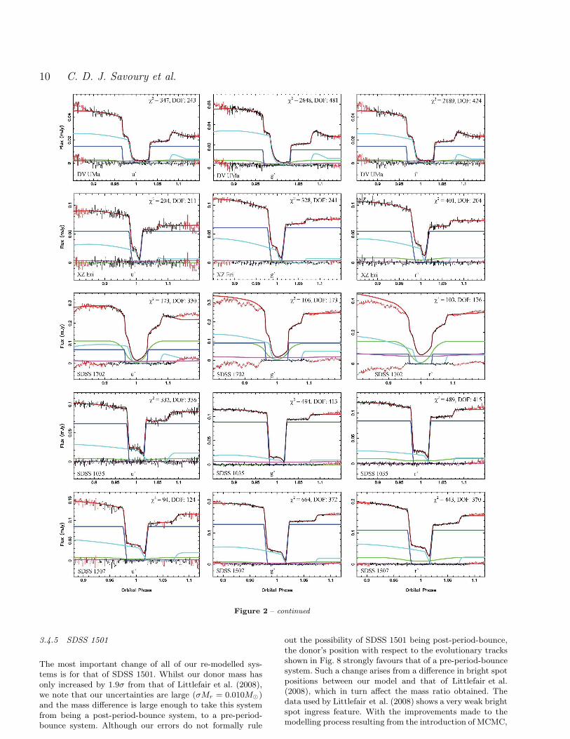
Figure 2. The phased-folded u′g′r′ or u′g′i′ light curves of the CVs listed in Table 3, fitted using the model outlined in section 3.3.The data (black) are shown with the fit (red) overlaid and the residuals plotted below (black). Below are the separate light curves of thewhite dwarf (dark blue), bright spot (light blue), accretion disc (green) and the secondary star (purple). Data points omitted from thefit are shown in red. χ2 values for each fit, together with the number of degrees of freedom (DOF) are also shown.

3.4.4 SDSS 1502

Our new fits to SDSS 1502 decrease the donor mass by2.9σ (∆Mr = 0.012M⊙) from that of Littlefair et al. (2008).Our mass ratio and inclination are consistent with those ofLittlefair et al. (2008), however our white dwarf radius, Rw,has increased by 13 percent (3.4σ). We believe the primary

reason for this change was that the original fit was heavilybinned, and thus more susceptible to the bug outlined insection 3.3.


Figure 2 – continued

3.4.5 SDSS 1501

The most important change of all of our re-modelled sys-tems is for that of SDSS 1501. Whilst our donor mass hasonly increased by 1.9σ from that of Littlefair et al. (2008),we note that our uncertainties are large (σMr = 0.010M⊙)and the mass difference is large enough to take this systemfrom being a post-period-bounce system, to a pre-period-bounce system. Although our errors do not formally rule

out the possibility of SDSS 1501 being post-period-bounce,the donor’s position with respect to the evolutionary tracksshown in Fig. 8 strongly favours that of a pre-period-bouncesystem. Such a change arises from a difference in bright spotpositions between our model and that of Littlefair et al.(2008), which in turn affect the mass ratio obtained. Thedata used by Littlefair et al. (2008) shows a very weak brightspot ingress feature. With the improvements made to themodelling process resulting from the introduction of MCMC,



it is clear that the 2006 data used by Littlefair et al. (2008)does not constrain the mass ratio, q, tightly enough. In con-trast, the 2004 data shows much clearer bright spot features,and we therefore favour this over the 2006 data as discussedin section 3.3.

4 DISCUSSION

4.1 White dwarf masses

Population studies by Willems et al. (2005) predict that be-tween 40 and 80 percent of CVs are born with He-corewhite dwarfs (Mw . 0.50M⊙) and therefore He-core whitedwarfs (He-WDs) are expected to be common amongst CVprimaries. It is surprising then that out of our sample of14 systems, we observe no He-WDs. Of all of our objects,


Figure 3. The white dwarf colours derived from our model fitted together with the white dwarf models of Bergeron et al. (1995). Fromtop to bottom, each curve represents log g = 9.0, 8.5, 8.0, 7.5 and 7.0 respectively. The measured white dwarf colours are shown here inred, and are used to derive the white dwarf temperature, which in turn is used to correct the white dwarf mass-radius relationships usedlater to obtain the final system parameters.

SDSS 1152 is found to have to the lowest white dwarfmass with Mw = 0.560 ± 0.028. The mass distribution ofKepler et al. (2007) for SDSS white dwarfs suggests He-WDs have a typical mass of ∼0.38M⊙. The most massiveHe-WDs are thought to form from single RGB stars, whichdue to extreme mass loss are able to avoid the Helium flash;D’Cruz et al. (1996) consider models with a range of mass

loss rates on the RGB and manage to produce He-WDs withmasses up to ∼0.48M⊙. It is likely that this represents anupper limit to the mass of He-WDs and hence SDSS 1152is too massive to be a viable candidate for a He-core whitedwarf.

We find that our white dwarf masses are not only toomassive to be He-WDs, but are also well in excess of the aver-


Figure 4. The normalised probability density functions for each system, derived using the MCMC chains, orbital period and the mass–radius relationships of Wood (1995), Panei et al. (2000) and Hamada & Salpeter (1961), at the appropriate white dwarf temperature.The red curve represents the r′ or i′ band fit, the green represents the g′ band, and blue curve (where present) represents the u′ band.The black represents the total, combined PDF. Shown are the PDFs for mass ratio q, white dwarf radius Rw/R⊙, donor mass Mr/M⊙,and inclination i◦.

age mass for single DA white dwarfs. Using the same methodas Knigge (2006), we calculated the average white dwarfmass of our entire sample to be Mw = 0.81± 0.04M⊙, withan intrinsic scatter of 0.13M⊙. In comparison, Liebert et al.(2005) find the mean mass of DA white dwarfs to beMw ∼0.603 M⊙, while Kepler et al. (2007) find a mean massof Mw = 0.593 ± 0.016M⊙.

Our study thus supports previous findings (e.g.Warner 1973, 1976; Ritter 1976, 1985; Robinson 1976;

Smith & Dhillon 1998; Knigge 2006) that white dwarfs inCVs are on average much higher in mass than single fieldstars. Like Littlefair et al. (2008), we compare our masses tothe average mass of Mw = 0.73 ± 0.05M⊙ for white dwarfsin CVs below the period gap (Knigge 2006) and find thatour white dwarf masses are generally much higher. This isespecially so for systems Porb 6 95 mins, where we find amean white dwarf mass of Mw = 0.83 ± 0.02M⊙, with anintrinsic scatter of 0.07M⊙. Some our white dwarf masses



Figure 6. Our g′ band observations of CTCV 2354 from 2009 (left), 2010 May 3 (centre) and 2010 June 6 (right), fit with a modifiedversion of the model obtained from the 2007 data as described in section 3.4.2.

are revised, and have accordingly moved downwards in masscompared to Littlefair et al. (2008), but as Fig. 7 shows, forPorb 6 95 mins, 8 out of 9 systems are more massive thanthe average found by Knigge (2006), with SDSS 1502 theonly exception. On the same plot, we also plot the disper-sion of masses as found by Knigge (2006) and the mean massof single SDSS white dwarfs found by Kepler et al. (2007).Note that the Knigge (2006) sample contains three systemsalso included in our study: OU Vir, DV UMa and XZ Eri,using the old mass determinations of Feline et al. (2004a,2004b). We see most of our masses are within the dispersionfound, indicating that no individual white dwarf mass is un-usual. However 8 out of 9 systems above average does seem

anomalously high, considering that if we model the whitedwarf masses as a Gaussian distribution, the probability ofsuch an occurrence is less than 2 percent (independent ofthe actual mean or variance). Such difference between oursample and that of Knigge (2006) is concerning, and it istherefore desirable to consider the selection effects, consid-ering the majority of our short period systems are all SDSSobjects (Szkody et al. 2004, 2005, 2006, 2007).

The majority of SDSS CVs found are generally rejectedquasar candidates with a limiting magnitude of g′ = 19−20,and are initially selected for follow up on the basis of u′-g′

colour cuts (see Gansicke et al. (2009) for a more in depthdescription). Littlefair et al. (2008) show that systems with


Mw > 0.50M⊙ are blue enough to pass the SDSS colour cutsand conclude that selection effects such as these are unlikelyto explain the high mass bias of our white dwarf sample.However, the majority of the systems we have studied areclose (g′∼ 17.5− 19.5) to the g′ = 19 limit of the SDSS sur-vey. This raises the possibility that the SDSS sample onlyfinds the brightest of the short period CVs. Ritter & Burkert(1986) have shown that CVs with high mass white dwarfsare brighter than their low mass counterparts. This suggeststhere maybe some bias towards high mass dwarfs. However,this conclusion is not appropriate to the systems studiedhere: Ritter & Burkert (1986) only consider the effects of ac-cretion luminosity whereas in most of our systems the whitedwarf considerably outshines the accretion disc.

Zorotovic et al. (2011) consider selection effects in whitedwarf dominated SDSS systems with a variety of differ-ent mass transfer rates and conclude there is actually biasagainst high mass white dwarfs. They find a 0.90M⊙ whitedwarf is approximately 0.15 magnitudes fainter than a0.75M⊙ white dwarf, which corresponds to a decreased de-tection efficiency of ∼ 20%. This suggests that our finding ofhigh mass white dwarfs at short orbital periods is not due toselection effects, and is in fact a true representation of theintrinsic mass distribution of CVs. However, this analysisonly considers white dwarf luminosity; in some of our sys-tems the bright spot features are prominent, and contributesignificantly to the overall flux of the system. It remainspossible that the finding of very high white dwarf massesfor our short period CVs is due to selection effects. How-ever, a full and thorough quantification of any bias wouldrequire detailed calculations of the luminosity of white-dwarfdominated systems (including bright spot emission) plus aninvestigation of the selection effects in the SDSS sample.Such an analysis is beyond the scope of this paper.

Our results have important consequences for the mod-elling of nova outbursts and their impact on the long-termevolution on CVs. Typical calculations show that the massof the white dwarf decreases by between 1 and 5 percentper 1000 nova cycles (e.g. Yaron et al. 2005; Epelstain et al.2007). The dominance of high-mass white dwarfs in our sam-ple of short period systems suggests that any white dwarferosion due to nova explosions must be minimal, or thatnot all of the accreted matter is ejected during nova ig-nition, resulting in the white dwarf mass increasing overtime. This could, in principle enable the white dwarfs incataclysmic variables to grow in mass until they reach theChandrasekhar limit.

4.2 Period bounce

Population synthesis models for cataclysmic variables (e.g.Kolb 1993; Willems et al. 2005) all predict that large num-bers of the CV population (∼15 - 70 percent) have evolvedpast the period minimum. This has always been in starkcontrast to observations, possibly in part due to selectioneffects (e.g. Littlefair et al. 2003).

Littlefair et al. (2006b, 2007, 2008) identified four sys-tems (SDSS 1035, SDSS 1507, SDSS 1433, SDSS 1501) withdonors below the sub-stellar limit, three of which are likelyto be post-period-bounce CVs (SDSS 1035, SDSS 1501 andSDSS 1433). Our subsequent re-analysis gives three systems(SDSS 1035, SDSS 1507, SDSS 1433) with donors below

the sub-stellar limit, two of which (for reasons outlined be-low) we believe are post-period-bounce CVs (SDSS 1035 andSDSS 1433). SDSS 1501, which no longer features as a post-period-bounce system, is discussed in greater detail in sec-tion 3.4.5.

Sirotkin & Kim (2010) claim that SDSS 1433 cannotbe considered a post-period-bounce object since the masstransfer rates and donor star temperatures implied are toohigh. The mass transfer rate is found using an estimate ofthe white dwarf temperature (Townsley & Gansicke 2009),while the donor star temperature is inferred using a semi-empirical relationship that is also dependent on the whitedwarf temperature. The white dwarf temperature used bySirotkin & Kim (2010) is that derived by Littlefair et al.(2008) from model fitting. We believe, at least in this case,that using M and T2 is an unreliable test of the evolutionarystatus of CVs donors, since accurate determinations of thewhite dwarf temperature are difficult to obtain. Of all thesystem parameters we have derived, the white dwarf tem-peratures are the least well constrained, and this does nottake into account systematic errors. Since the white dwarftemperature is found using the flux from just three colours,and our model does not include all possible sources of lumi-nosity (e.g. a boundary layer), there is a good chance ourwhite dwarf temperatures are affected by systematic errorsat some level, as discussed in section 3.3. Instead, we focuson the donor star mass, Mr.

If the angular momentum loss rate is similar for sys-tems with identical system parameters, we expect all CVsto follow very similar evolutionary tracks with a single lo-cus in the mass-period relationship (and by analogy, mass-radius relationship) for CV donors, as shown in Fig. 8.The empirical donor star mass-radius relationship derivedby Knigge (2006) shows that a single evolutionary trackdoes very well at describing the observed M2−Porb relation-ship, although the shape of that relationship is poorly con-strained at low masses. A single evolutionary path also ex-plains the presence of the “period spike”, a long sought afterfeature in the orbital period distribution recently identifiedby Gansicke et al. (2009). We therefore expect there to bea unique donor mass corresponding to the minimum orbitalperiod, below which an object becomes a period-bouncer.The exact mass at which this occurs is very uncertain,and does not necessarily correspond to the sub-stellar limit(Patterson 2009). From the empirical work of Knigge (2006),the best estimate for Mbounce is Mr = 0.063 ± 0.009M⊙.Three of our systems (SDSS 1035, SDSS 1433 and SDSS1507) fall well below this value, although SDSS 1507 is anunusual system, and is discussed in the following section. Asin Littlefair et al. (2008), we do not include it in our sampleof post-period minimum CVs. We therefore have two strongcandidates for post-period minimum CVs (SDSS 1035 andSDSS 1433) from our total sample of 14 CVs (nine of whichare SDSS systems). From this, we estimate that 14± 7 per-cent of all CVs below the period gap, and 22 ± 11 percentof all short period CVs (Porb 6 95 mins) have evolved pastthe period minimum. These findings are consistent, albeitto a crude approximation given our small sample of objects,with current population synthesis models. Since all of ourshort period systems are SDSS CVs, we cannot rule out se-lection effects, but Gansicke et al. (2009) have shown thatthe number of period minimum CVs found within the SDSS


Figure 7. White dwarf mass as a function of orbital period. The mean white dwarf mass for systems below the period gap, as found byKnigge (2006) is shown with a solid line, along with the associated intrinsic scatter (dashed line). The mean white dwarf mass in singlestars as found by Kepler et al. (2007) is shown by a dotted line.

is broadly consistent with other surveys, allowing for nor-malisation of survey volumes.

4.3 SDSS 1507

The orbital period of SDSS 1507 is far below the well-defined period minimum and thus the nature of this systemis of great interest to theorists and observers. It is possiblethat this system represents the true orbital period minimumas predicted by Kolb & Baraffe (1999). However, if this isindeed the case, we would expect a large number of sys-tems between orbital periods of 67 minutes, and 83 minuteswhere the period spike is observed (Gansicke et al. 2009).These systems are not observed, and hence it is likely thatsome other mechanism is responsible. Littlefair et al. (2007)speculate that this system was either formed directly froma white dwarf/brown dwarf binary, while Patterson et al.(2008) argue that the system could be a member of the halo.Both derive system parameters, and both obtain distanceestimates to the system.

Our derived system parameters are consistent withthose of Littlefair et al. (2007) and Patterson et al. (2008),within uncertainties. Our distance estimate is in excellentagreement with Littlefair et al. (2007), which is not supris-ing since we both calculate the distance using the samemethods and dataset. However, our new distance estimatestill places the system nearer than that of Patterson et al.(2008). Patterson et al. (2008) obtain a lower limit to thedistance using parallax. The parallax value implies a dis-tance d > 175 pc, which taken alone, is consistent with

our estimate of d = 168 ± 12 pc. Patterson combines hisparallax with a range of other observational constraints us-ing Bayesian methods to yield a final distance estimate ofd = 230± 40 pc. If our distance of d = 168± 12 pc is nearerthe true distance, then combining with Patterson’s propermotion measurement of 0.16′′/yr yields a transverse velocityof d = 128± 9 kms−1. This lower transverse velocity is stillvery much an outlier in the distribution of 354 CVs shownin Fig.1 of Patterson et al. (2008). Therefore, regardless ofwhich distance is correct, the proper motion of SDSS 1507still supports halo membership.

4.4 Exploring the standard model of CV evolution

Fig. 8 shows the evolutionary models of Kolb & Baraffe(1999) calculated with enhanced mass-transfer rates. Alsoshown is a model with 50 percent star spot coverage on thesurface of the donor. Positions of the period minimum, andperiod gap as found by Knigge (2006) are also shown. Massdeterminations for all systems presented here are included.We see that the standard theoretical models are a poor fitto the data. For a given mass, the models of Kolb & Baraffe(1999) significantly underestimate the orbital period, andthus the donor radii.

Models with enhanced mass transfer rates and star spotcoverage do rather better at reproducing the observed donormasses, although the general scatter of short period systemsmakes choosing between these difficult. This is in line withthe conclusions of Littlefair et al. (2008). The models be-gin to diverge significantly at orbital periods greater than


100 minutes. Unfortunately, in this regime there are few sys-tems with precisely known donor masses. Clearly, we requiremore mass determinations for systems with orbital periodsbetween 100 and 130 minutes.

5 CONCLUSIONS

We present high-speed, three-colour photometry of a sampleof 14 eclipsing CVs. Of these CVs, nine are short period(Porb 6 95 minutes), and one is within the period gap. Foreach of the 14 objects we determine the system parametersby fitting a physical model of the binary to the observedlight curve by χ2 minimisation. We find that two of our nineshort period systems appear to have evolved past the periodminimum, and thus supports various assertions that between15 and 70 per cent of the CV population has evolved past theorbital period minimum. The donor star masses and radii arenot consistent with model predictions, with the majorityof donor stars being ∼10 per cent larger than predicted.Our derived masses and radii show that this can explainedby either enhancing themass transfer rate or modifying thestellar physics of the donor star to take into account star spotcoverage. Unfortunately, we still lack enough precise donormasses between orbital periods of 100 and 130 minutes tochoose between these alternatives.

Finally, we find that the white dwarfs in our sampleshow a strong tendency towards high masses. The high massdominance implies that the white dwarfs in CVs are notsignificantly eroded by nova outbursts, and may actuallyincrease over several nova cycles. We find no evidence forHe-core white dwarfs within our sample, despite predictionsthat between 40 and 80 percent of short period CVs shouldcontain He-core white dwarfs.

6 ACKNOWLEDGEMENTS

We would like to thank our referee, Joe Patterson for hisuseful comments. We also thank Christian Knigge for usefuldiscussions on white dwarf bias and selection effects. CDJSacknowledges the support of an STFC PhD. SPL acknowl-edges the support of an RCUK Fellowship. CMC and TRMare supported under grant ST/F002599/1 from the Scienceand Technology Facilities Council (STFC). ultracam andultraspec are supported by STFC grant ST/G003092/1.This research has made use of NASA’s Astrophysics DataSystem Bibliographic Services. This article is based on ob-servations made with ultracam mounted on the Isaac New-ton Group’s WHT, and ultracam and ultraspecmountedon the European Southern Observatory’s NTT and VLTtelescopes.

REFERENCES

Bergeron P., Wesemael F., Beauchamp A., 1995, PASP,107, 1047

Chabrier G., Gallardo J., Baraffe I., 2007, A&A, 472, L17Copperwheat C., Marsh T., Dhillon V., Littlefair S., Hick-man R., Gansicke B., Southworth J., 2010, MNRAS, 402,1824

D’Cruz N., Dorman B., Rood R., O’Connell R., 1996, ApJ,446, 359

Dhillon V., et al 2007, MNRAS, 378, 825

Epelstain N., Yaron O., Kovetz A., Prialnik D., 2007, MN-RAS, 374, 1449

Feline W., 2005, PhD thesis, The University of Sheffield

Feline W., Dhillon V., Marsh T., Stevenson M., Watson C.,Brinkworth C., 2004a, MNRAS, 347, 1173

Feline W., Dhillon V., Marsh T., Brinkworth C., 2004b,MNRAS, 355, 1

Ford E., 2006, ApJ, 642, 505

Gansicke B., Dillon M., Southworth J., Thornstensen J.,Rodrıguez-Gil P., Aungwerojwit A., Marsh T., et al. 2009,MNRAS, 397, 2170

Gregory P., 2007, MNRAS, 381, 1607

Hamada T., Salpeter E., 1961, ApJ, 134, 683

Hellier C., 2001, Cataclysmic Variable Stars. Praxis Pub-lishing Ltd, Chichester

Horne K., Marsh T., Cheng F., Hubany I., Lanz T., 1994,ApJ, 426, 294

Kepler S., Kleinman S., Nitta A., Koester D., CastanheiraB., Giovannini O., Althaus L., 2007, in Napiwotzki R.,Burleigh M., eds, 15th European Workshop on WhiteDwarfs Vol. 372 of ASPCS, The white dwarf mass dis-tribution. pp 35–40

Knigge C., 2006, MNRAS, 373, 484

Kolb U., 1993, A&A, 271, 149

Kolb U., Baraffe I., 1999, MNRAS, 309, 1034

Liebert J., Bergeron P., Holberg J., 2005, ApJS, 156, 47

Littlefair S., Dhillon V., Martn E., 2003, MNRAS, 340, 264

Littlefair S., Dhillon V., Marsh T., Gansicke B., 2006a,MNRAS, 371, 1435

Littlefair S., Dhillon V., Marsh T., Gansicke B., South-worth J., Watson C., 2006b, Sci, 314, 1578

Littlefair S., Dhillon V., Marsh T., Gansicke B., Baraffe I.,Watson C., 2007, MNRAS, 381, 827

Littlefair S., Dhillon V., Marsh T., Gansicke B., South-worth J., Baraffe I., Watson C., Copperwheat C., 2008,MNRAS, 388, 1582

Paczynski B., 1981, Acta Astron., 31, 1

Panei J., Althaus L., Benvenuto O., 2000, A&A, 353, 970

Patterson J., 1998, PASP, 110, 1132

Patterson J., 2009, ArXiv e-prints

Patterson J., Thornstensen J., Knigge C., 2008, PASP, 120,510

Pickles A., 1998, PASP, 110, 863

Ritter H., 1976, MNRAS, 175, 279

Ritter H., 1985, A&A, 148, 207

Ritter H., Burkert A., 1986, A&A, 158, 161

Roberts G., Gelman A., Gilks W., 1997, Annual of AppliedProbability, 7, 110

Robinsons E. L., 1976, ApJ, 203, 485

Sirotkin F. V., Kim W.-T., 2010, ApJ, 721, 1356

Smith D., Dhillon V., 1998, MNRAS, 301, 767

Smith J., et al. 2002, AJ, 123, 2121

Southworth J., Copperwheat C. M., Gansicke B. T., PyrzasS., 2010, A&A, 510, A100+

Szkody P., et al. 2004, ApJ, 128, 1882

Szkody P., et al. 2005, ApJ, 129, 2386

Szkody P., et al. 2006, ApJ, 131, 973

Szkody P., et al. 2007, ApJ, 134, 185


Figure 8. The M2−Porb relationship for our dataset. Mass determinations for all systems using ultracam data are included. Our threenew systems, in addition to other objects of particular interest are labelled. The evolutionary models of Kolb & Baraffe (1999) calculatedwith different mass-transfer rates are shown with red (dashed) and blue (dot-dashed) lines. A model with 50 percent star spot coverageon the surface of the donor is shown with an orange (dotted) line. The solid (black) line shows the empirical mass-radius relationship asfound by Knigge (2006). The position of the period minimum and period gap, as found by Knigge (2006), are also shown.

Tappert C., Augusteijn T., Maza J., 2004, MNRAS, 354,321

Townsley D., Gansicke B., 2009, ApJ, 693, 1007Tulloch S., Rodrıguez-Gil P., Dhillon V., 2009, MNRAS,397, L82

Warner B., 1973, MNRAS, 162, 189Warner B., 1976, in IAU Symposium, Vol.73, Structure andEvolution of Close Binary Systems, ed. P. Eggleton, S.Mitton & J.Whelan, 85-+

Warner B., 1995, Cataclysmic Variable Stars. CambridgeUniversity Press, Cambridge

Willems B., Kolb U., Sandquist E., Taam R., Dubus G.,2005, ApJ, 635, 1263

Wood J., Irwin M., Pringle J., 1985, MNRAS, 214, 475Wood J., Horne K., Berriman G., Wade R., O’DonoghueD., Warner B., 1986, MNRAS, 219, 629

Wood M., 1995, in Koester D., Werner K., eds, LNP Vol.443, White Dwarfs. Springer-Verlag, Berlin. p.41

Yaron O., Prialnik D., Shara M., Kovetz A., 2005, ApJ,623, 398

Zorotovic, M., Schriber. M.R., Gansicke., B.T., 2011, A&A,submitted

Cataclysmic variables below the period gap: mass...

Documents

Transcript of Cataclysmic variables below the period gap: mass...