CassandraUser Manual

for version 1.0.0, 5 August 2008

Joris Peeters

This manual is for Cassandra (version 1.0.0, 5 August 2008).

Copyright c© 2007, 2008 Joris Peeters. Copyright c© 2007, 2008 Ghent University.

Permission is granted to make and distribute verbatim copies of this manualprovided the copyright notice and this permission notice are preserved on allcopies.

Permission is granted to copy and distribute modified versions of this manualunder the conditions for verbatim copying, provided that the entire resultingderived work is distributed under the terms of a permission notice identical tothis one.

Permission is granted to copy and distribute translations of this manual intoanother language, under the above conditions for modified versions, exceptthat this permission notice may be stated in a translation approved by the FreeSoftware Foundation.

i

Table of Contents

1 Introduction . . . . . . . . . . . . . . . . . . . . . . . . . . . . . . . . . . . . . 1

2 Tutorial . . . . . . . . . . . . . . . . . . . . . . . . . . . . . . . . . . . . . . . . . . 22.1 Configuration files . . . . . . . . . . . . . . . . . . . . . . . . . . . . . . . . . . . . . . . . . . . . . . 2

2.1.1 config.dat . . . . . . . . . . . . . . . . . . . . . . . . . . . . . . . . . . . . . . . . . . . . . . . . . 22.1.2 Geometry file . . . . . . . . . . . . . . . . . . . . . . . . . . . . . . . . . . . . . . . . . . . . . . 42.1.3 Impressed currents file . . . . . . . . . . . . . . . . . . . . . . . . . . . . . . . . . . . . . 52.1.4 External field file . . . . . . . . . . . . . . . . . . . . . . . . . . . . . . . . . . . . . . . . . . 52.1.5 Output configuration file . . . . . . . . . . . . . . . . . . . . . . . . . . . . . . . . . . 6

2.2 Output . . . . . . . . . . . . . . . . . . . . . . . . . . . . . . . . . . . . . . . . . . . . . . . . . . . . . . . . 72.2.1 Field output files . . . . . . . . . . . . . . . . . . . . . . . . . . . . . . . . . . . . . . . . . . 72.2.2 Geometry output files . . . . . . . . . . . . . . . . . . . . . . . . . . . . . . . . . . . . . 72.2.3 Current output files . . . . . . . . . . . . . . . . . . . . . . . . . . . . . . . . . . . . . . . 7

3 Installation instructions for Cassandra . . . . . . . . 93.1 Installation on GNU/Linux . . . . . . . . . . . . . . . . . . . . . . . . . . . . . . . . . . . . . 9

3.1.1 Pre-requisitions for Cassandra (GNU/Linux) . . . . . . . . . . . . . . . 93.1.1.1 FFTW . . . . . . . . . . . . . . . . . . . . . . . . . . . . . . . . . . . . . . . . . . . . . . . . . 93.1.1.2 BLAS and LAPACK . . . . . . . . . . . . . . . . . . . . . . . . . . . . . . . . . . . . . 9

3.1.2 Installation of Cassandra . . . . . . . . . . . . . . . . . . . . . . . . . . . . . . . . . 113.1.3 Parallel Cassandra . . . . . . . . . . . . . . . . . . . . . . . . . . . . . . . . . . . . . . . 12

3.2 Installation on Windows (Cygwin) . . . . . . . . . . . . . . . . . . . . . . . . . . . . . 143.2.1 Pre-requisitions for Cassandra (Cygwin) . . . . . . . . . . . . . . . . . . 14

3.3 Configure options for Cassandra . . . . . . . . . . . . . . . . . . . . . . . . . . . . . . . 14

4 Testing your installation . . . . . . . . . . . . . . . . . . . . . . 16

5 Acknowledgments . . . . . . . . . . . . . . . . . . . . . . . . . . . . . 17

6 License and Copyright . . . . . . . . . . . . . . . . . . . . . . . . 18

Chapter 1: Introduction 1

1 Introduction

This manual documents version 1.0.0 of Cassandra, a three-dimensional full-wave electro-magnetic solver for scattering at large and complicated dielectric and perfectly conductingobjects. Its features include,

• A number of predefined incoming field excitations as well as impressed current excita-tion.

• The ability to handle complicated structures, including recursively embedded objectsand objects having a shared boundary (junctions).

• Automatic meshing for a number of simple geometries and a flexible input system foruser-defined triangular meshes.

• Fast and memory-efficient solution of large problems through use of theNSPW-MLFMA algorithm, stable at all frequencies.

• Sequential solution of multiple right-hand sides (excitations).• Extensive output possibilities for the generation of far fields, near fields, RCS, ...• The possibility of parallel solution for very large problems, relying on the generic Nexus

framework for asynchronous parallel treatment of fast multipole methods.

We will assume that you are familiar with the basics of electromagnetism and the numericalmethods, namely Method of Moments and ML-FMA. This is a an early release of thesoftware and might still contain some bugs. Also note that we do not take any responsibilityregarding the correctness of the results and neither can we be held responsible for anydamage our software might inflict on your system.

The Cassandra software project is being developed as a research tool by Joris Peeters, whilepursuing his PhD.

Chapter 2: Tutorial 2

2 Tutorial

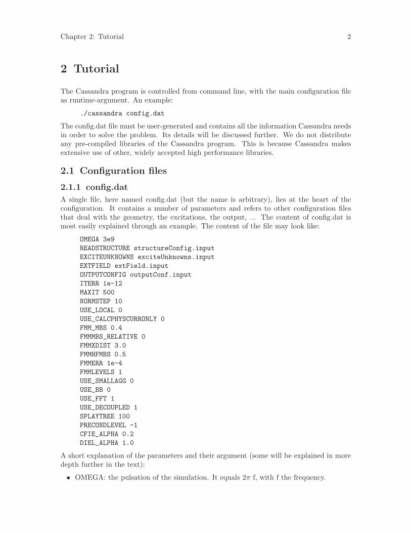
The Cassandra program is controlled from command line, with the main configuration fileas runtime-argument. An example:

./cassandra config.dat

The config.dat file must be user-generated and contains all the information Cassandra needsin order to solve the problem. Its details will be discussed further. We do not distributeany pre-compiled libraries of the Cassandra program. This is because Cassandra makesextensive use of other, widely accepted high performance libraries.

2.1 Configuration files

2.1.1 config.dat

A single file, here named config.dat (but the name is arbitrary), lies at the heart of theconfiguration. It contains a number of parameters and refers to other configuration filesthat deal with the geometry, the excitations, the output, ... The content of config.dat ismost easily explained through an example. The content of the file may look like:

OMEGA 3e9READSTRUCTURE structureConfig.inputEXCITEUNKNOWNS exciteUnknowns.inputEXTFIELD extField.inputOUTPUTCONFIG outputConf.inputITERR 1e-12MAXIT 500NORMSTEP 10USE_LOCAL 0USE_CALCPHYSCURRONLY 0FMM_MBS 0.4FMMMBS_RELATIVE 0FMMXDIST 3.0FMMHFMBS 0.5FMMERR 1e-4FMMLEVELS 1USE_SMALLAGG 0USE_BB 0USE_FFT 1USE_DECOUPLED 1SPLAYTREE 100PRECONDLEVEL -1CFIE_ALPHA 0.2DIEL_ALPHA 1.0

A short explanation of the parameters and their argument (some will be explained in moredepth further in the text):

• OMEGA: the pulsation of the simulation. It equals 2π f, with f the frequency.

Chapter 2: Tutorial 3

• READSTRUCTURE: refers to the file containing the geometry.• EXCITEUNKNOWNS: refers to the file specifying the impressed currents.• EXTFIELD: refers to the file specifying the external (applied) fields.• OUTPUTCONFIG: refers to the file specifying the form of output to be calculated.• ITERR: the relative error on the solution vector, resulting from the iterative solution.• MAXIT: the maximum number of iterations (set to -1 for unlimited)• NORMSTEP: the number of iterations between calculation of the relative error. Setting

this to a large number will speed up the iterations by approximately 30%, but mayobviously result in more iterations than necessary.

• USE LOCAL: indicates whether or not to use local geometry. It saves memory to doso, but right now should not be used in combination with impressed currents.

• USE CALCPHYSCURRONLY: after every simulation the currents will be stored in afile. The program uses an equivalent current formulation for solution and these currentsare only physical in the case of a PEC. This parameter indicates whether to output allcurrents or only those at a PEC interface.

• FMM MBS: the size of the minimal box at the lowest level of the Fast Multipole Three.• FMMMMBS RELATIVE: indicates whether or not the FMMMBS is relative to the

wavelength or in absolute values (meters).• FMMXDIST: the minimal distance between group centra (in units of MBS) for inter-

actions to be treated as far. This distance may be increased slightly (followed by awarning) by the program, when it’s a number that can cause numerical difficulties.

• FMMHFMBS: the minimal size (in units of wavelengths) for a box to be treated withthe High Frequent MLFMA.

• FMMERR: the required (maximal) relative error on the interactions calculated throughFMM. More accuracy leads to long calculations and more memory. Less accuracy leadsto more inaccurate solution and possibly to divergence of the solution.

• FMMLEVELS: the number of FMM levels used. 0 indicates a 1 level FMM. Use -1 toindicate that you wish to use a pure Method of Moments.

• USE SMALLAGG: indicates whether or not to use small aggregation matrices (basedon the fact that you don’t need the full bandwidth at aggregation time). Choosing thisoption will lead to significant memory gain but comes with a small price in terms ofreduced speed, due to some additional interpolation.

• USE BB: indicates whether or not to use the broadband system (excellent at lowerfrequencies)

• USE FFT: indicates whether or not to use the high frequent formulation. When bothUSE FFT ands USE BB are 1, the program will make an optimal choice.

• USE DECOUPLED: indicates whether or not to use the decoupled aggregation pat-terns (speeds up the interpolation in the BB-case)

• SPLAYTREE: indicates the size (in MB) of the splaytree. The splaytree is a system toefficiently extract symmetry in the near interaction elements. A bigger splay tree canextract more identical interactions but takes up more memory.

• PRECONDLEVEL: indicates the FMM level which should be directly inverted for useas a blockdiagonal preconditioner. -1 means there will be no preconditioner.

Chapter 2: Tutorial 4

• CFIE ALPHA: for closed PEC objects the CFIE formulation is used, which is acombination of α EFIE (ill-conditioned but highly accurate) and (1-α )MFIE (well-conditioned but less accurate). The parameter indicates the alpha used.

• DIEL ALPHA: for dielectrics a linear combination as α PMCHWT (ill-conditionedbut highly accurate) + (1-α )nMuller (well-conditioned but less accurate) is used. Theparameter indicates the alpha used.

Some parameters are not strictly required and will receive default values when they areomitted from the config.dat file, but it is recommended to include all of them. The followingsections will deal with the additional configuration files.

2.1.2 Geometry file

This file is referred to as the argument of READSTRUCTURE in the config.dat file. Itcontains all the necessary information to build the geometrical structure (i.e. the mesh ofthe environment). A small number of meshes (for a cuboid, sphere and plate) can be createdby Cassandra, but more complex structures need to be meshed with an outside programand then fed to Cassandra through a mesh-file. Its construction is again best demonstratedby means of a small example:

MEDIUM DIELECTRIC 1.0 0.0 1.0 0.0BOUNDARY PLATE 5 -3 -3 5 3 -3 5 -3 3 0.5MEDIUM PEC VOIDBOUNDARY SPHERE 0.0 0.0 0.0 1.0 0.2MEDIUM DIELECTRIC 2.0 0.0 1.0 0.0BOUNDARY FILE airplane.mshMEDIUM PEC CLOSED

There are two main commands: MEDIUM and BOUNDARY, respectively (and sequen-tially) denoting the addition of a medium and the boundary (mesh) of a medium. The twocommands should always be alternated. First a boundary is created with BOUNDARY andthen the inside of the boundary is filled with the medium indicated on the next line. Thefirst boundary must be omitted because it is always infinite space. So in this example wefill the background medium with vacuum (epsR=1+0i, muR=1+0i), we then include a 6x6plate at x=5, discretised with triangles of typical size 0.5. This plate is then indicated to bea void PEC (an open surface). On the next line we define a sphere, centered at the origin,with radius 1.0 and discretisation 0.2, which is then filled with a dielectric with epsR=2.0and muR=1.0. Finally an airplane is added through a file, which is defined as a closedPEC object. The mesh file for the airplane must be in a certain format. The first linecontains the number of boundaries (always 1 here), for backwards-compatibility purposes.The second line contains the number of vertices and the number of triangles, for instance’1000 1500’. The following lines (in this case 1000) each contain three number specifyingthe x y z coordinates of the vertices. The file ends with (in this case) 1500 lines that eachcontain three numbers (e.g. 1 2 3) referring to the indices of the vertices that make upthe triangle (note that the order of the indices will influence the direction of the normal).Cassandra automatically takes care of extracting junctions or embedding objects. Beware,however, that the program will only be able to construct a junction if both boundariescontain identical (save for some numerical error) triangles (in terms of the vertices, not

Chapter 2: Tutorial 5

necessarily their order). There is additional support for the mesh output format of the GiDmeshing program. Files generated with GiD can be added through

BOUNDARY GID filename

Adding a plate or cuboid is done by supplying, respectively, three or four points that definethe structure, shaped like an axis system with the origin as the first point. The syntax forboth is thus,

BOUNDARY PLATE x1 y1 z1 x2 y2 z2 x3 y3 z3 dBOUNDARY CUBOID x1 y1 z1 x2 y2 z2 x3 y3 z3 x4 y4 z4 d

with, in both cases, d the typical size of the triangles. Note that this formulation allows forthe use of skewed plates and cuboids.

A sphere is added through

BOUNDARY SPHERE x y z R d

with (x,y,z) the center, R the radius and d the discretisation size. Note that meshing asphere with plane triangles always leads to a certain amount of geometrical discretisationerror.

2.1.3 Impressed currents file

This file is referred to as the argument of EXCITEUNKNOWNS in the config.dat. Afterconstruction of the basis functions (consisting of two triangles), Cassandra checks withinthe impressed currents whether one of the basis functions has an applied coefficient. Thiswould remove this basis function from the list of unknowns and add it to the right hand.Right now, configuration of this is still a little awkward. An example,

12 0.01 0.01 2 0.08 0.08 0 1 0

might make things more clear. The first line of the file indicates the number of impressedbasis functions. The second line contains a unique definition of the basis function. First,two (x,y,z) coordinates are supplied, which each lie in on of the two triangles making up thebasis function. The following number is the medium in which this basis function lies. Thisis important in some cases, namely when two basis function have the same triangles butindependent coefficient, for instance when the junction between two dielectrics is a PECplate. Right now, do not use any impressed currents in combination with USE LOCAL 1.

2.1.4 External field file

This file is referred to as the argument of EXTFIELD in the config.dat. It is responsible foradding applied fields to the simulation. The geometry of the source is not included in thesimulation. A number of typical external fields is supplied. Each line in the file containsthe definition of an external field (e.g. a plane wave, dipole, gaussian beam, .. ). Sequentialexternal fields will be added to the same right hand, until the keyword ’STOP’ is detected,after which a new right hand is constructed. A small example, with two right hands:

FIELD 0 PLANEWAVE 0 0 -1 0 0 1 0 0 0STOPFIELD 0 PLANEWAVE 1 0 0 0 0 0 0 1 0

Chapter 2: Tutorial 6

FIELD 0 PLANEWAVE 0 1 0 0 0 0 0 1 0STOP

The first right hands contains only one external field, namely a Y-polarised plane wavetravelling in the negative z-direction. The second right hand contains two orthogonallytravelling plane waves with a z-polarisation. The number right after the keyword ’FIELD’indicates the medium in which the external field is present. 0 always refers to the backgroundmedium. A small overview of currently supported external fields.

• PLANEWAVE kx ky kz ExR ExI EyR EyI EzR EzIA planewave travelling in the (kx,ky,kz) direction with complex amplitude(ExR+iExI,EyR+iEyI,EzR+iEzI) for the electric field.

• DIPOLE x y z JxR JxI JyR JyI JzR JzIA (small) dipole, centered at (x,y,z) with (JxR+iJxI,JyR+iJyI,JzR+iJzI) as the complexamplitude of the current density at the center. Internally, the dipole is constructed asa combination of three vectormultipoles.

• GAUSSIANBEAM x y z kx ky kz ExR ExI EyR EyI EzR EzI wA gaussian beam, origin at (x,y,z), travelling in the (kx,ky,kz) direction with withcomplex amplitude (ExR+iExI,EyR+iEyI,EzR+iEzI) for the electric field and waist w.Note that this is a very rudimentary implementation of gaussian beams that will onlylead to physically correct results in the vicinity of the origin.

• VECTORMULTIPOLE x y z l m typeMN typejh Ar AiA vectormultipole, located at (x,y,z) and of order l,m. typeMN can be M or N toindicate the type, while typejh can be j or h, to indicate which bessel function is used(first kind or hankel). The complex amplitude is Ar+iAi.

• DELTAGAP x y z ExR ExI EyR EyI EzR EzIA delta-gap excitation, located at x,y,z and with complex amplitude(ExR+iExI,EyR+iEyI,EzR+iEzI) for the electric field. Note that this delta-gap will only have an effect when (x,y,z) lies within a triangle of the mesh.

2.1.5 Output configuration file

This file is referred to as the argument of OUTPUTCONF in the config.dat. It definesthe outputs that need to be calculated for each right hand. Note that it is not possible toconfigure a different output-format for different right hands. An example

FIELD pointsCASE.input ET.out TOTALFIELD pointsCASE.input EI.out INCOMINGFIELD pointsRECT.input ET2D.out TOTAL

The first argument of FIELD indicates the list of points at which to which to calculate theoutput. This coordinates file should be in the following format

nPointsx1 y1 z1x2 y2 z2..

The second argument denotes the name of the outputfile. Note that i is added at the endof the filename to indicate the result of various right hands. For instance, the first output

Chapter 2: Tutorial 7

result for the third righthand would be named ET.out 2 (counting starts at zero). Thefinal parameter indicates the type of field to be calculated, either TOTAL, INCOMING orSCATTERED.

2.2 Output

2.2.1 Field output files

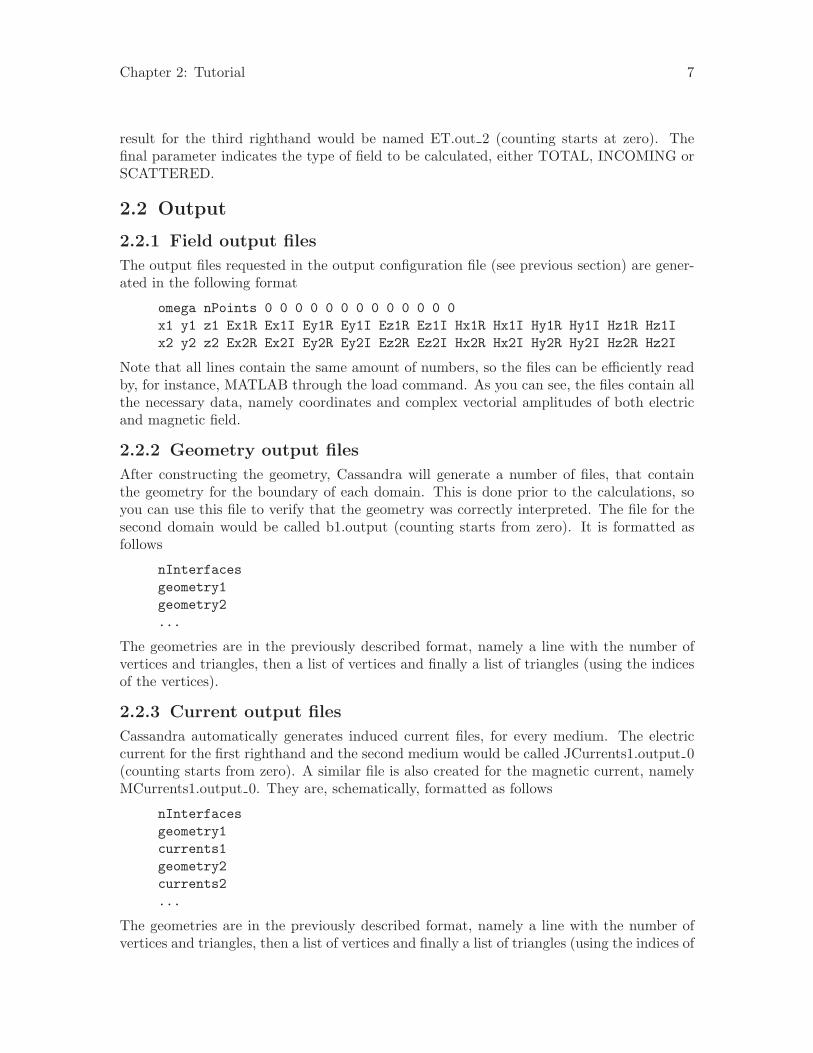
The output files requested in the output configuration file (see previous section) are gener-ated in the following format

omega nPoints 0 0 0 0 0 0 0 0 0 0 0 0 0x1 y1 z1 Ex1R Ex1I Ey1R Ey1I Ez1R Ez1I Hx1R Hx1I Hy1R Hy1I Hz1R Hz1Ix2 y2 z2 Ex2R Ex2I Ey2R Ey2I Ez2R Ez2I Hx2R Hx2I Hy2R Hy2I Hz2R Hz2I

Note that all lines contain the same amount of numbers, so the files can be efficiently readby, for instance, MATLAB through the load command. As you can see, the files contain allthe necessary data, namely coordinates and complex vectorial amplitudes of both electricand magnetic field.

2.2.2 Geometry output files

After constructing the geometry, Cassandra will generate a number of files, that containthe geometry for the boundary of each domain. This is done prior to the calculations, soyou can use this file to verify that the geometry was correctly interpreted. The file for thesecond domain would be called b1.output (counting starts from zero). It is formatted asfollows

nInterfacesgeometry1geometry2...

The geometries are in the previously described format, namely a line with the number ofvertices and triangles, then a list of vertices and finally a list of triangles (using the indicesof the vertices).

2.2.3 Current output files

Cassandra automatically generates induced current files, for every medium. The electriccurrent for the first righthand and the second medium would be called JCurrents1.output 0(counting starts from zero). A similar file is also created for the magnetic current, namelyMCurrents1.output 0. They are, schematically, formatted as follows

nInterfacesgeometry1currents1geometry2currents2...

The geometries are in the previously described format, namely a line with the number ofvertices and triangles, then a list of vertices and finally a list of triangles (using the indices of

Chapter 2: Tutorial 8

the vertices). Following every geometry is a list (as long as the list of triangles) of vectorialcomplex amplitudes that indicate the current at the centroid of the corresponding triangle.

Chapter 3: Installation instructions for Cassandra 9

3 Installation instructions for Cassandra

3.1 Installation on GNU/Linux

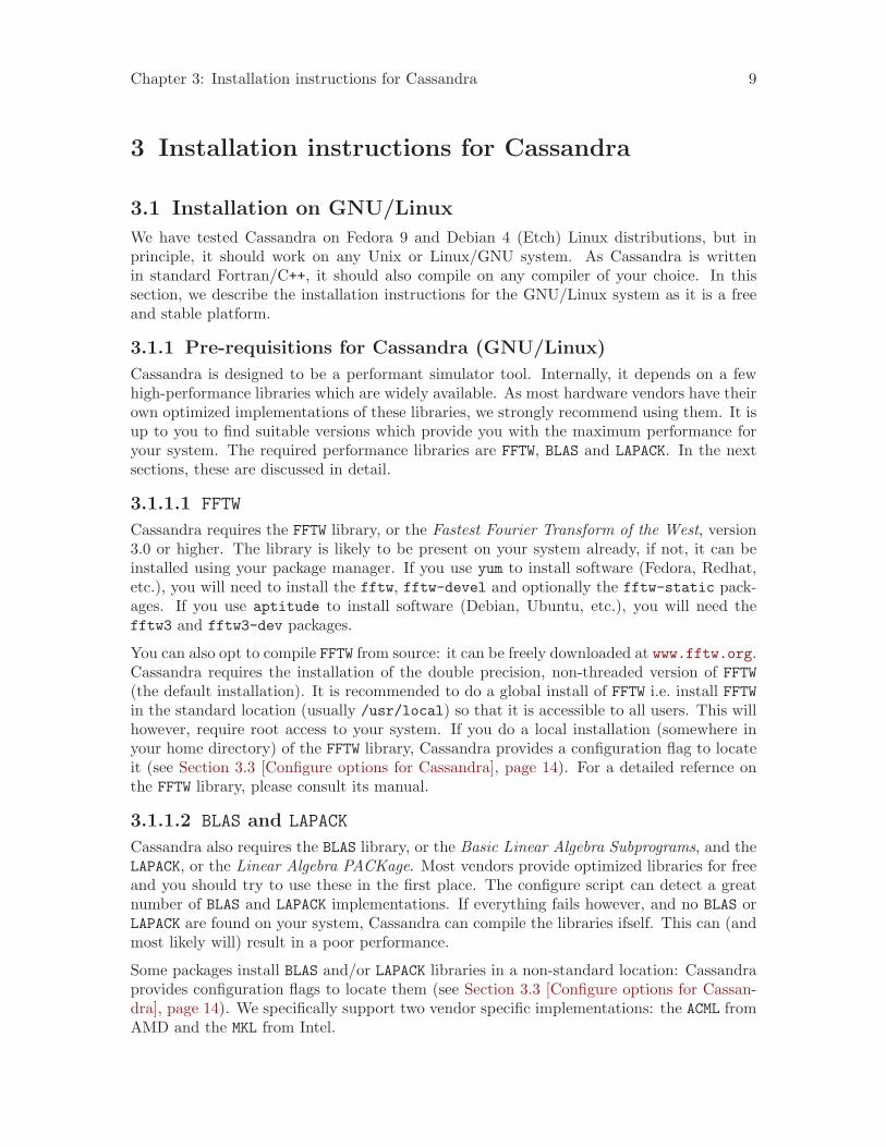
We have tested Cassandra on Fedora 9 and Debian 4 (Etch) Linux distributions, but inprinciple, it should work on any Unix or Linux/GNU system. As Cassandra is writtenin standard Fortran/C++, it should also compile on any compiler of your choice. In thissection, we describe the installation instructions for the GNU/Linux system as it is a freeand stable platform.

3.1.1 Pre-requisitions for Cassandra (GNU/Linux)

Cassandra is designed to be a performant simulator tool. Internally, it depends on a fewhigh-performance libraries which are widely available. As most hardware vendors have theirown optimized implementations of these libraries, we strongly recommend using them. It isup to you to find suitable versions which provide you with the maximum performance foryour system. The required performance libraries are FFTW, BLAS and LAPACK. In the nextsections, these are discussed in detail.

3.1.1.1 FFTW

Cassandra requires the FFTW library, or the Fastest Fourier Transform of the West, version3.0 or higher. The library is likely to be present on your system already, if not, it can beinstalled using your package manager. If you use yum to install software (Fedora, Redhat,etc.), you will need to install the fftw, fftw-devel and optionally the fftw-static pack-ages. If you use aptitude to install software (Debian, Ubuntu, etc.), you will need thefftw3 and fftw3-dev packages.

You can also opt to compile FFTW from source: it can be freely downloaded at www.fftw.org.Cassandra requires the installation of the double precision, non-threaded version of FFTW(the default installation). It is recommended to do a global install of FFTW i.e. install FFTWin the standard location (usually /usr/local) so that it is accessible to all users. This willhowever, require root access to your system. If you do a local installation (somewhere inyour home directory) of the FFTW library, Cassandra provides a configuration flag to locateit (see Section 3.3 [Configure options for Cassandra], page 14). For a detailed refernce onthe FFTW library, please consult its manual.

3.1.1.2 BLAS and LAPACK

Cassandra also requires the BLAS library, or the Basic Linear Algebra Subprograms, and theLAPACK, or the Linear Algebra PACKage. Most vendors provide optimized libraries for freeand you should try to use these in the first place. The configure script can detect a greatnumber of BLAS and LAPACK implementations. If everything fails however, and no BLAS orLAPACK are found on your system, Cassandra can compile the libraries ifself. This can (andmost likely will) result in a poor performance.

Some packages install BLAS and/or LAPACK libraries in a non-standard location: Cassandraprovides configuration flags to locate them (see Section 3.3 [Configure options for Cassan-dra], page 14). We specifically support two vendor specific implementations: the ACML fromAMD and the MKL from Intel.

Chapter 3: Installation instructions for Cassandra 10

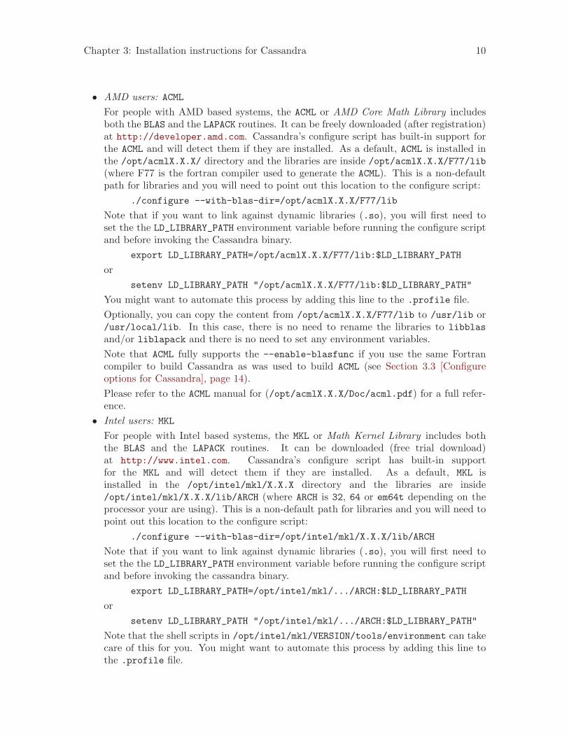
• AMD users: ACML

For people with AMD based systems, the ACML or AMD Core Math Library includesboth the BLAS and the LAPACK routines. It can be freely downloaded (after registration)at http://developer.amd.com. Cassandra’s configure script has built-in support forthe ACML and will detect them if they are installed. As a default, ACML is installed inthe /opt/acmlX.X.X/ directory and the libraries are inside /opt/acmlX.X.X/F77/lib(where F77 is the fortran compiler used to generate the ACML). This is a non-defaultpath for libraries and you will need to point out this location to the configure script:

./configure --with-blas-dir=/opt/acmlX.X.X/F77/lib

Note that if you want to link against dynamic libraries (.so), you will first need toset the the LD_LIBRARY_PATH environment variable before running the configure scriptand before invoking the Cassandra binary.

export LD_LIBRARY_PATH=/opt/acmlX.X.X/F77/lib:$LD_LIBRARY_PATH

orsetenv LD_LIBRARY_PATH "/opt/acmlX.X.X/F77/lib:$LD_LIBRARY_PATH"

You might want to automate this process by adding this line to the .profile file.Optionally, you can copy the content from /opt/acmlX.X.X/F77/lib to /usr/lib or/usr/local/lib. In this case, there is no need to rename the libraries to libblasand/or liblapack and there is no need to set any environment variables.Note that ACML fully supports the --enable-blasfunc if you use the same Fortrancompiler to build Cassandra as was used to build ACML (see Section 3.3 [Configureoptions for Cassandra], page 14).Please refer to the ACML manual for (/opt/acmlX.X.X/Doc/acml.pdf) for a full refer-ence.

• Intel users: MKL

For people with Intel based systems, the MKL or Math Kernel Library includes boththe BLAS and the LAPACK routines. It can be downloaded (free trial download)at http://www.intel.com. Cassandra’s configure script has built-in supportfor the MKL and will detect them if they are installed. As a default, MKL isinstalled in the /opt/intel/mkl/X.X.X directory and the libraries are inside/opt/intel/mkl/X.X.X/lib/ARCH (where ARCH is 32, 64 or em64t depending on theprocessor your are using). This is a non-default path for libraries and you will need topoint out this location to the configure script:

./configure --with-blas-dir=/opt/intel/mkl/X.X.X/lib/ARCH

Note that if you want to link against dynamic libraries (.so), you will first need toset the the LD_LIBRARY_PATH environment variable before running the configure scriptand before invoking the cassandra binary.

export LD_LIBRARY_PATH=/opt/intel/mkl/.../ARCH:$LD_LIBRARY_PATH

orsetenv LD_LIBRARY_PATH "/opt/intel/mkl/.../ARCH:$LD_LIBRARY_PATH"

Note that the shell scripts in /opt/intel/mkl/VERSION/tools/environment can takecare of this for you. You might want to automate this process by adding this line tothe .profile file.

Chapter 3: Installation instructions for Cassandra 11

Optionally, you can copy the content from /opt/intel/mkl/VERSION/lib/ARCH to/usr/lib or /usr/local/lib. In this case, there is no need to rename the libraries tolibblas and/or liblapack and there is no need to set any environment variables.Note that MKL fully supports the --enable-blasfunc if you use the same Fortrancompiler to build Cassandra as was used to build MKL. In practice, we have noted (inversion 10.0.1) that MKL supports the g77 Fortran calling conventions and not thoseof gfortran. You are advised to compile Cassandra using the g77 compiler if youcan. However, it appears that the --enable-blasfunc is fully compatible with thecombination of gfortran and MKL. The configure script will issue a warning, but onour test system, everything went smooth. Be carefull however that this might just beluck.

• Compile your own BLAS/LAPACK (not recommended)If no BLAS and/or LAPACK are found on your system, Cassandra will compile theselibraries from source. This can however, result in a poor performance. Pleasenote that the source files inside the directory src/zofpack/machcons need tobe compiled without any sort of optimization. This is forced by overriding the$FFLAGS variable and setting them to empty for that directory. If you should havea Fortran compiler with default optimization turned on, you will need to editsrc/zofpack/machcons/Makefile.am manually and set the $FFLAGS to disable thisoptimization. You will need to rerun automake first to regenerate the Makefiles.

3.1.2 Installation of Cassandra

Cassandra comes with a configure script in the GNU style. Installation can be as simpleas:

./configuremakemake install

This will build the non-MPI flavor of Cassandra and will install it in the standard place.This typically requires root privileges. To specify a different install directory use the --prefix flag to configure.

./configure --prefix=yourinstalldirectory

If you have problems during configuration or compilation, you may want to run make cleanbefore trying again; this ensures that you don’t have any files left over from previous com-pilation attempts.

Cassandra is written in C++ but internally compiles two or more Fortran-77 libraries: AMOS,PIM and optionally BLAS and LAPACK). If you link against pre-build (optimized) BLAS andLAPACK libaries, you must use a compatible Fortran compiler (including compiler options)with our software as were used to compile BLAS/LAPACK. To specify a specific Fortrancompiler use e.g. for the g77 compiler

./configure F77=g77

or

./configure F77=gfortran

Chapter 3: Installation instructions for Cassandra 12

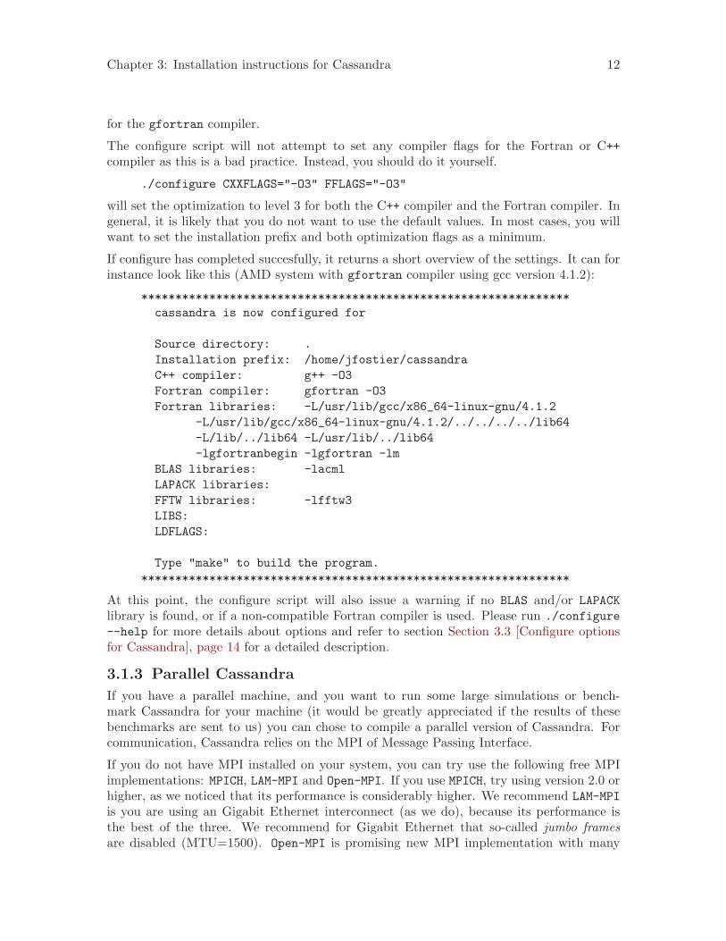
for the gfortran compiler.

The configure script will not attempt to set any compiler flags for the Fortran or C++compiler as this is a bad practice. Instead, you should do it yourself.

./configure CXXFLAGS="-O3" FFLAGS="-O3"

will set the optimization to level 3 for both the C++ compiler and the Fortran compiler. Ingeneral, it is likely that you do not want to use the default values. In most cases, you willwant to set the installation prefix and both optimization flags as a minimum.

If configure has completed succesfully, it returns a short overview of the settings. It can forinstance look like this (AMD system with gfortran compiler using gcc version 4.1.2):

***************************************************************cassandra is now configured for

Source directory: .Installation prefix: /home/jfostier/cassandraC++ compiler: g++ -O3Fortran compiler: gfortran -O3Fortran libraries: -L/usr/lib/gcc/x86_64-linux-gnu/4.1.2

-L/usr/lib/gcc/x86_64-linux-gnu/4.1.2/../../../../lib64-L/lib/../lib64 -L/usr/lib/../lib64-lgfortranbegin -lgfortran -lm

BLAS libraries: -lacmlLAPACK libraries:FFTW libraries: -lfftw3LIBS:LDFLAGS:

Type "make" to build the program.***************************************************************

At this point, the configure script will also issue a warning if no BLAS and/or LAPACKlibrary is found, or if a non-compatible Fortran compiler is used. Please run ./configure--help for more details about options and refer to section Section 3.3 [Configure optionsfor Cassandra], page 14 for a detailed description.

3.1.3 Parallel Cassandra

If you have a parallel machine, and you want to run some large simulations or bench-mark Cassandra for your machine (it would be greatly appreciated if the results of thesebenchmarks are sent to us) you can chose to compile a parallel version of Cassandra. Forcommunication, Cassandra relies on the MPI of Message Passing Interface.

If you do not have MPI installed on your system, you can try use the following free MPIimplementations: MPICH, LAM-MPI and Open-MPI. If you use MPICH, try using version 2.0 orhigher, as we noticed that its performance is considerably higher. We recommend LAM-MPIis you are using an Gigabit Ethernet interconnect (as we do), because its performance isthe best of the three. We recommend for Gigabit Ethernet that so-called jumbo framesare disabled (MTU=1500). Open-MPI is promising new MPI implementation with many

Chapter 3: Installation instructions for Cassandra 13

nice options and features (like support for multiple Gigabit Ethernet connections to a sin-gle machine). At the time of writing, it is however still a bit slower than its LAM-MPIcounterpart.

The three MPI implementations can be freely downloaded

• LAM-MPI www.lam-mpi.org

• MPICH www.mcs.anl.gov/mpi/mpich

• Open-MPI www.open-mpi.org

After installation, add the directory to the MPI compiler scripts to the PATH environment(you will need the C++ MPI compiler, usually called mpic++, mpicxx or mpiCC). Theconfigure script will try to detect the correct one. To enable MPI support in Cassandra addthe --enable-mpi flag to the configure script.

./configure --enable-mpi

As is previously described (see Chapter 2 [Tutorial], page 2), Cassandra requires two inputfiles, namely the config.dat script and the input geometry file (.igf). In a parallel envi-ronment, it is required that all processes have access to these files so they can be read inparallel. Most likely, some sort of network file system is mounted on each machine, so allthe machines see the same files. If this is not the case, you must make sure that the twoinput files are locally available on each machine in the same path. Make sure that all inputfiles are identical!. If this requirement is not met, Cassandra will crash once it starts itsiterations.

We have noticed that when using a network file system, it might take a few seconds beforethe changes made to a file on one machine propagate to the other machines (most likelysome buffering issues). Future versions of Cassandra will communicate a fingerprint of theinput files to make sure that they are all identical.

If you want to do some serious benchmarking, we suggest using the benchmarks which comealong with Cassandra and are located in /share/benchmark. You might want to read theREADME file first.

Cassandra can also be compiled with MPE support. Using the MPE library, bottleneckscan be detected in a post-mortem fashion. The MPE library is included in MPICH, but canbe downloaded separately www-unix.mcs.anl.gov/perfvis and used in combination withLAM-MPI and Open-MPI. To enable support for MPE in Cassandra, use the --enable-mpeflag

./configure --enable-mpi --enable-mpe

To launch a parallel job, use the mpirun tool

mpirun -np xx ./cassandra config.dat

Change xx by the number of processes you want to use. To specify which machines touse, you most likely want to create a so-called machinefile which contains their names orip-numbers. We refer to the user’s guide of your MPI implementation of choice.

Chapter 3: Installation instructions for Cassandra 14

3.2 Installation on Windows (Cygwin)

The installation on Windows is as straightforward as the installation on GNU/Linux thanksto Cygwin. Cygwin is an environment which emulates Unix or Linux behaviour on Windows.Only the serial version (one processor) of Cassandra, however, is available under Windows.Note that the performance under Cygwin can be dramatically lower than on GNU/Linux.Therefore, we only recommend Windows systems for testing purposes.

3.2.1 Pre-requisitions for Cassandra (Cygwin)

You will need to install Cygwin on your Windows machine first. We have tested withWindows XP and Cygwin v. 2.573.2.2 but we don’t expect any problems on other sytems.In addition to the base installation, you will need to select the following packages:

Under Devel

• gcc-g++: C++ compiler• gcc-g77: Fortran compiler• make: The GNU version of the ‘make’ utility• libtool: A shared library generation tool

Under Math

• lapack: Comprehensive FORTRAN library for linear algebra operations.• libfftw3-devel: Discrete Fourier transform library (development)

Some of these packages will automatically trigger the installation of their dependencies.This is a good thing. The installation is then exactly performed in the same manner asdescribed in section Section 3.1.2 [Installation of Cassandra], page 11.

You can still use the configure options as explained in section Section 3.3 [Configure optionsfor Cassandra], page 14, except for

• --enable-mpi

• --enable-mpe

• --enable-blasfunc

as the first two involve the use of MPI and the latter doesn’t appear to work will withCygwin.

3.3 Configure options for Cassandra

The configure script supports all the standard flags defined by the GNU Coding Standards;see the INSTALL file in Cassandra or the GNU web page. Note especially --help to list allflags. The configure script also accepts a few Cassandra-specific flags, particularly:

• --enable-debug Build Cassandra with some debugging checks turned on. Note thatenabling this setting will alter any compilation flags. If you want to add for instance"-g3" to the compiler flags, please change CXXFLAGS and/or FFLAGS.

• --enable-mpi This will compile the MPI version of Cassandra. Note that even for theMPI version of Cassandra, you do not need the MPI version of FFTW.

Chapter 3: Installation instructions for Cassandra 15

• --enable-mpe This will compile Cassandra with MPE logging support. If requires thelibmpe and liblmpe libraries. The resulting output file can then be examined withjumpshot. Note that this flag requires also the --enable-mpi flag to be enabled.

• --enable-blasfunc By default, Cassandra does not call any BLAS functions (it doeshowever, call several BLAS subroutines). This is because of the fact that differentFortran compilers have different conventions for returning the function’s resulting value.Enabling this flag will force Cassandra to call the BLAS functions anyway. This islikely somewhat faster. In our experience, you can safely use this flag in quality BLASimplementations (e.g. ACML and MKL). The configure script will perform a few tests andwarn the user if it suspects any trouble.

• --with-fftw-dir=<DIR> Use this flag if you have a local installation of the FFTW li-brary. Note that you need to provide the base directory in which you install FFTW(the same directory you used as a prefix when you compiled FFTW). The actual FFTWlibraries will then be located in $(basedir)/lib and the include file (fftw3.h) in$(basedir)/include.

• --with-blas-dir=<DIR> Use this flag to specify the directory in which the BLAS libraryis located.

• --with-blas=<DIR> Specify the name of the BLAS library. Note that if you use thisflag, no other BLAS libraries will be considered. This flag can be used to force thecompilation of the BLAS library from source by setting it to an empty value.

• --with-lapack-dir=<DIR> Use this flag to specify the directory in which the LAPACKlibrary is located.

• --with-lapack=<LIB> Specify the name of the LAPACK library. Note that if you usethis flag, no other LAPACK libraries will be considered. This flag can be used to forcethe compilation of the LAPACK library from source by setting it to an empty value.

Chapter 4: Testing your installation 16

4 Testing your installation

Cassandra comes with a small number of examples that were pre-calculated. These can beused to test your installation. There are currently four tests (described below), in the /tests/directory after unpacking. You can run a test by copy-pasting your compiled executableinto one of the test-directories (for instance /tests/test1/) and run

./cassandra config.dat

After the simulation, Cassandra will automatically compare the result with the referencesolution and indicate the relative error. This error does not need to be zero, because thetests are not with infinite precision. In fact, relative errors below 1e-3 indicate a successfultest. A small description of the tests

• test1: A very simple and small PEC cube, calculated without any FMM.• test2: A very simple and small dielectric cube, calculated without any FMM.• test3: A long PEC strip, calculated with high frequent ML-FMA.• test4: A dielectric cube, at low frequency, calculated with the NSPW-MLFMA (requires

about 3GB of RAM).

The tests are designed to include different aspects of what might go wrong. If all tests aresuccesful, chances are very high that your installation is OK. The tests can be run bothin single processor and parallel mode. If you wish to run them in parallel mode, be sureto include a machine file. In addition, you could even make small modification to someparameters in the config.dat of the tests to observe the behaviour. For instance, increasingthe accuracy of the FMM should still lead to a correct result. Note, however, that changingthe frequency will obviously no longer allow a comparison with the pre-calculated solution.

Chapter 5: Acknowledgments 17

5 Acknowledgments

We thank SourceForge.net for providing us with a reliable SubVersion (SVN) server and awebsite. We are especially grateful to the maintainers of SourceForge for helping us out onseveral occasions.

We are grateful for all the efforts of our system administrator Bert De Vuyst. His countlessinterventions saved the day numerous times.

We thank Jan Fostier, author of Nexus and Nero2D, for support and for writing the manualfor Nero2D, from which we copy-pasted quite shamelessly.

We thank the GNU/Linux community for providing us with the tools we needed in thedevelopment of our software.

We thank the creators of the FFTW software (Steven Johnson and Mateo Frigo), for pro-viding us with a reliable tools for fast calculation of the DFTs. We are also grateful to themfor providing us with a texinfo template we used for creating this manual.

We thank the authors of the Parallel Iterative Methods or PIM (Rudnei Dias da Cunha)for their software.

We thank the authors of the AMOS library (Donald E. Amos) for his library for the calcu-lation of special functions.

Prof. Femke Olyslager stimulated us in creating this software as GNU package to the com-munity. We are of course, grateful for that.

Chapter 6: License and Copyright 18

6 License and Copyright

Cassandra is Copyright c© 2007, 2008 Joris Peeters, Copyright c© 2007, 2008 Ghent Uni-versity, department of Information Technology (INTEC).

Cassandra is free software; you can redistribute it and/or modify it under the terms of theGNU General Public License as published by the Free Software Foundation; either version2 of the License, or (at your option) any later version.

This program is distributed in the hope that it will be useful, but WITHOUT ANY WAR-RANTY; without even the implied warranty of MERCHANTABILITY or FITNESS FORA PARTICULAR PURPOSE. See the GNU General Public License for more details.

You should have received a copy of the GNU General Public License along with this program;if not, write to the Free Software Foundation, Inc., 59 Temple Place, Suite 330, Boston,MA 02111-1307 USA. You can also find the GPL on the GNU web site.