Case Studies in Trajectory Optimization: Trains, Planes ...rvdb/tex/trajopt/trajopt_OptEng.pdf ·...

Optimization and Engineering, 2, 215–243, 2001c© 2002 Kluwer Academic Publishers. Manufactured in The Netherlands.

Case Studies in Trajectory Optimization: Trains, Planes,and Other Pastimes

ROBERT J. VANDERBEIOperations Research and Financial Engineering, Princeton University, Princeton, NJ, USA

Received September 22, 2000; Revised September 17, 2001

Abstract. This is the first in a series of papers presenting case studies in modern large-scale constrainedoptimization, the purpose of which is to illustrate how recent advances in algorithms and modeling languageshave made it easy to solve difficult optimization problems using off-the-shelf software. In this first paper, weconsider four trajectory optimization problems: (a) how to operate a train efficiently, (b) how to putt a golf ball onan uneven green so that it arrives at the cup with minimal speed, (c) how to fly a hang glider so as to maximize orminimize the range of the glide, and (d) how to design a slide to make a toboggan go from beginning to end asquickly as possible.

In addition to the tutorial aspects of this paper, we also present evidence suggesting that the widely usedtrapezoidal discretization method is inferior in several ways to a certain simpler midpoint discretization method.

Keywords: trajectory optimization, optimal control, constrained optimization

1991 Mathematics Subject Classification: Primary 65L10 Secondary 34B15

1. Introduction

This is the first in a series of papers presenting case studies in constrained optimization. Thepurpose of these studies is to illustrate how recent advances in algorithms and modelinglanguages now make it easy to solve once difficult optimization problems using off-the-shelve software. A secondary goal is to show that it is nonetheless still possible to makesubtle errors in a model which will render it (a) more difficult than it needs to be or(b) infeasible or, worse, (c) feasible but giving the wrong answer. In the past, many of theoptimization problems we present here were thought to be very difficult to solve and it wasunclear whether failures were due to bad algorithms or bad models. Today, one can say thatfailures are almost always due to bad models.

In this paper we consider trajectory optimization problems. Our first example is abouthow to drive a train so as to minimize fuel costs. We follow this with two examples from theworld of sports: golfing and flying. Subsequent papers in this series will treat applications inelectrical engineering (filter and antennae-array design) and in civil engineering (topologyoptimization of structures).

Throughout the paper we present several optimization models. We express these modelsin the AMPL modeling language (Fourer et al., 1993). This language provides a commonmechanism for conveying problems to codes to solve them. When solving problems we

216 VANDERBEI

generally use two different solvers: (a) LOQO (Vanderbei, 1999a, 1999b; Vanderbei andShanno, 1999; Benson et al., 2000), which implements an interior-point method for generalnonlinear optimization and (b) SNOPT (Gill et al., 1997), which implements an active setstrategy with a quasi-Newton method for the QP subproblem.

This paper is intended to be a tutorial on trajectory optimization. We direct the interestedreader to John Betts’ book (Betts, 2000) for a much more in depth treatment.

2. Trains

An important problem in transportation is to minimize fuel costs in the operation of a train.To keep things simple, we consider a segment of track that is straight although it maycontain hills and valleys. Let x denote position along the track measured from some fixedreference point. Letting v denote the derivative of position with respect to time and a thetime-derivative of v, we arrive at the following equations describing the motion of the train:

v = x

a = v (1)

a = h(x) − (α + β|v| + γ v2) + ua − ub.

Here, h(x) represents the acceleration/deceleration caused by going down/up hills, α, β,and γ are constants so that the first two terms, α + β|v|, represent fricton per unit massdue to rolling on the track and the third term, γ v2, represents friction per unit mass due toair resistance, ua represents the acceleration provided by the engines, and ub represents thedeceleration from applying the brakes. The control variables are the functions ua and ub.The objective is to take the train from one place given by initial condition

x(0) = x0

v(0) = v0

to another given by

x(T ) = x f

v(T ) = v f

in such a way as to minimize fuel costs, which we take to be proportional to the total amountof work done:

∫ T

0ua(t)v(t)dt.

To get a specific instance of this problem, we take the initial position to be zero, the finalposition to be 6.0 km, the initial and final velocities to be zero, the total trip time to be 4.8minutes and

α = 0.3, β = 0.14, γ = 0.16.

TRAINS, PLANES, AND OTHER PASTIMES 217

Figure 1. The acceleration profile caused by hills. The first two miles are uphill, then there are two miles of flat,and the last two miles are downhill.

Finally, the hill function h is taken to be

h(x) =m−1∑j=1

(s j+1 − s j )1

πtan−1 x − z j

ε

where m represents the number of hill sections, s j is the slope along the j-th section, z j

is the breakpoint between the j-th and the j + 1-st section, and ε gives a spread which isrelated to the length of the train itself. Our specific choice involves an initial uphill climbfollowed by a level section and then a final downhill run. Hence, it has m = 3 and

z1 = 2, z2 = 4,

s1 = 2, s2 = 0, s3 = −2.

A plot of h is shown in figure 1.

2.1. Midpoint discretization method

This problem can be cast as a (nonconvex) nonlinear optimization problem by discretizingthe time interval [0, T ] into N small time intervals and writing discrete approximationsfor the derivatives that appear in the model. There are many ways to do this (see, e.g.,Carnahan et al., 1969 which discusses many methods including Runge-Kutta, Collocation,etc.). In this paper, we discuss two very simple discretizations: midpoint discretization1 andtrapezoidal discretization. We begin with the midpoint method. Letting x[j] denote thevalue of x at time jT/N,j=0,1,. . .,N, we define a discrete approximation to the velocityat the midpoint of each time interval as follows:

v[j+0.5] = (x[j+1]- x[j])/(T/N) j=0,1,. . .,N-1,

218 VANDERBEI

Figure 2. The AMPL model trainh.mod.

The discrete approximation for acceleration is defined similarly:

a[j] = (vx[j+0.5]-vx[j-0.5])/(T/N) j=1,. . .,N-1,

This approximation is called midpoint discretization. The equations of motion given by (1)can then be written as:

a[j] = h(x[j]) - (a+b*v[j]+c*v[j] ^2) + u_a[j] - u_b[j].

Of course, velocities are defined at the half-integer points yet we access values here at thewhole integer points. Hence, it is necessary to provide reasonable values for velocities atthese integer points; we use the average of the two nearest half-integer values. The completemodel expressing the midpoint discretization in the AMPL modeling language is shown infigure 2.

2.2. Ringing

A graph showing x , v, and a as functions of time is shown in figure 3. Note the “ringing”phenomenom apparent in the acceleration during times of medium acceleration. Such a


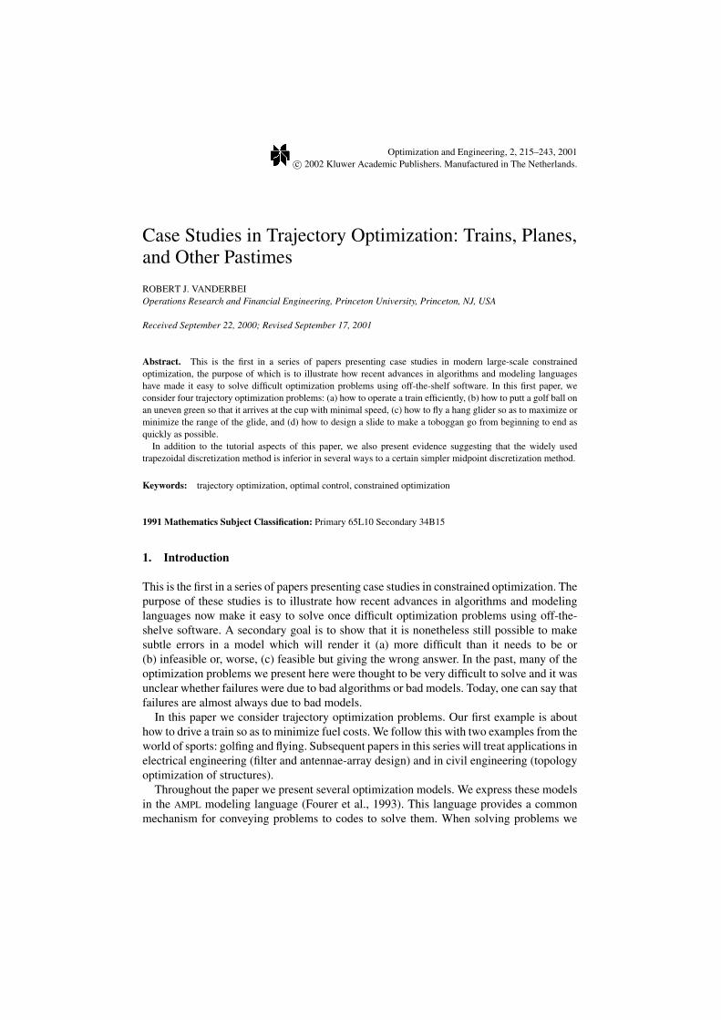
Figure 3. Output produced with N=201.

phenomenon suggests that something is wrong. To test whether it is a bug in the optimizationalgorithm, we solved the problem with two completely different solvers: LOQO and SNOPT.Both solvers produced similar ringing. We conclude that ringing is intrinsic to the model.Next, we refined the discretization to N=501 and solved the problem again. This time, LOQO

and SNOPT both exhibited ringing but it was much more pronounced in LOQO. The objectivefunctions matched out to the 8 digits of accuracy requested by the two solvers. (For thosewho like to keep score, LOQO solves the N=501 problem in 6.86 seconds and SNOPT requires35.71 seconds to solve the problem.)

Reflection sheds some light on what is happening. With a highly refined partition, acontrol scheme that alternates between two values becomes indistinguishable from one thatapplies the average of the two all the time. Imagine riding in a car with someone who pumpsthe gas pedal. The speed remains essentially constant and the rate of consumption of fuel isjust the average of the pumped and unpumped rates. Hence, other than making passengerssick, this control is just as good as a smooth one.

This reasoning suggests that the set of near optimal solutions is large. Sometimes interior-point methods get into trouble in such cases. In fact, trouble is assured if the set of optimalsolutions is unbounded. For the train problem, setting N=1001 LOQO finds a solution thatis accurate only to 3 digits whereas SNOPT still can get 8 digits (although it takes a longtime). Larger values of N cause even more trouble. Clearly ringing is bad for interior-pointmethods.

2.3. Smoothing

The model can be improved by adding to the objective some measure of the work of“pumping the pedal”. For example, after adding a tiny correction

1.0e-8 *sum {i in 1..N-2} (u[i+1] - u[i])^2/h

220 VANDERBEI

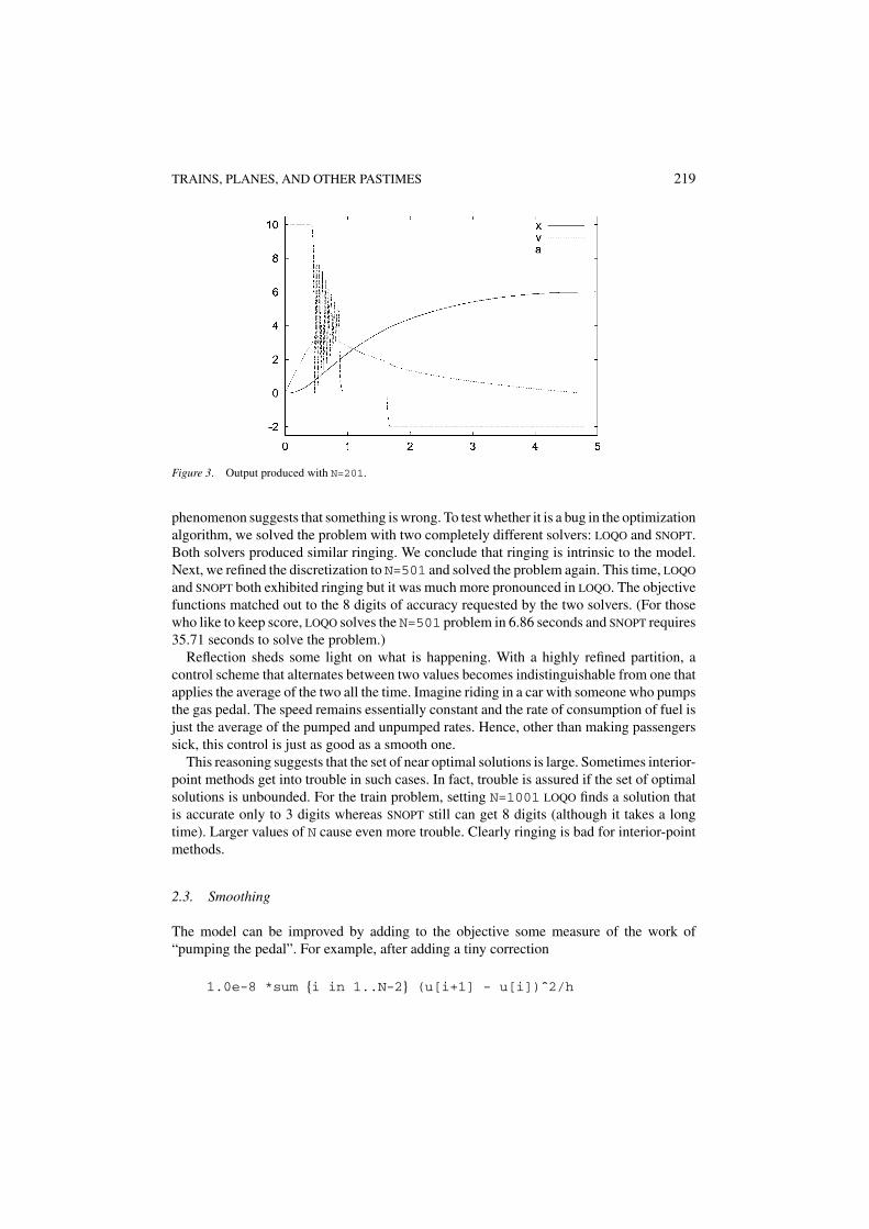
Figure 4. LOQO output produced with N=2001.

to the objective function in the model shown in figure 2, LOQO has no trouble solving theN=1001 case and gets an answer that exhibits no ringing whatsoever. The solution to theN=2001 case is shown in figure 4.

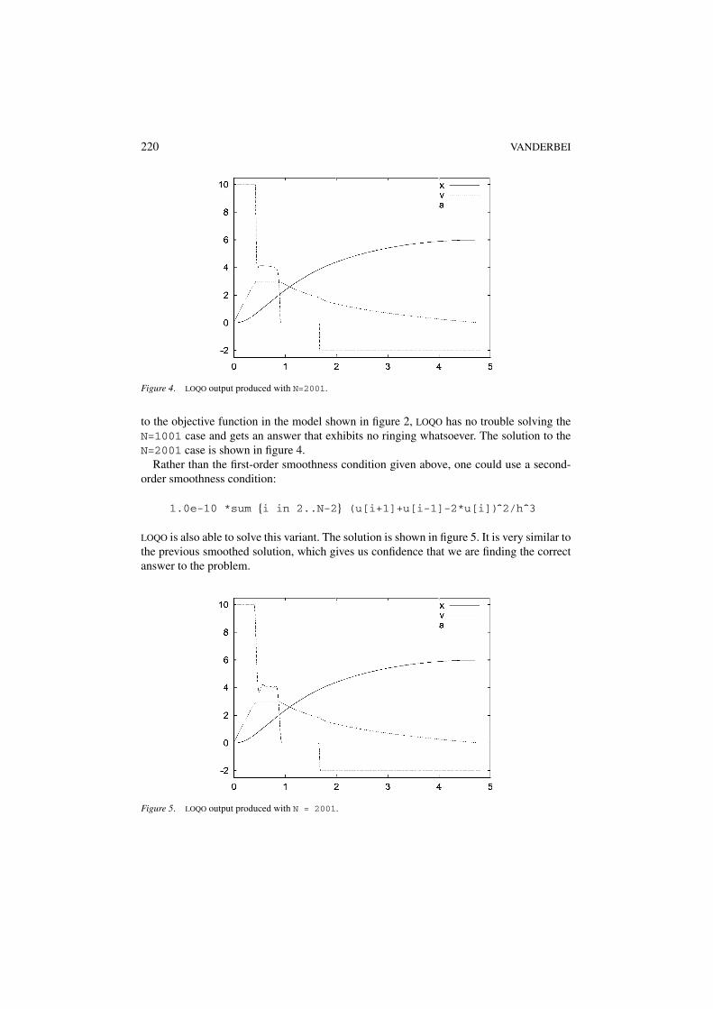
Rather than the first-order smoothness condition given above, one could use a second-order smoothness condition:

1.0e-10 *sum {i in 2..N-2} (u[i+1]+u[i-1]-2*u[i]) 2/h^3

LOQO is also able to solve this variant. The solution is shown in figure 5. It is very similar tothe previous smoothed solution, which gives us confidence that we are finding the correctanswer to the problem.

Figure 5. LOQO output produced with N = 2001.


We end here our discussion of ringing by remarking that this phenomenon is common; ithas nothing to do with the shape of the hills/valleys or with the initial and final conditions.In fact, one can see ringing even in the case where the entire track is level (i.e., h ≡ 0)and the initial and final velocities are both equal to the total distance divided by the totaltime. In this case, the optimal control should be static. That is, one should provide just theamount of acceleration needed to maintain the initial speed throughout the trip. But, withoutthe smoothing terms mentioned above, both LOQO and SNOPT find nonstatic ringing-typesolutions. For more on the ringing phenomenon and how to deal with it, we refer the readerto Meziat (2000).

2.4. Trapezoidal discretization

We end this section with a description of the second common method for discretizing first-order differential equations. This method is called the trapezoidal discretization. With thisdiscretization, values for v and a are defined at the same discrete times as for x; that is,at jT/N, j=0,1,. . .,N. Instead of giving a formula defining each velocity in terms of adifference of positions, we give constraints that say that the average value of the values ofv at two adjacent times is equal to the appropriate difference in the positional values:

(v[j+1]+v[j])/2 = (x[j+1]-x[j])/(T/N) j=0,1,...,N-1,

Constraints that must be satisfied by the accelerations are similar:

(a[j+1]+a[j])/2 = (v[j+1]-v[j])/(T/N) j=0,1,...,N-1,

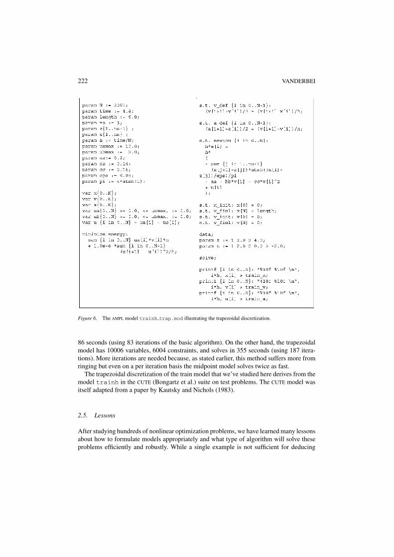
The model in its entirety is shown in figure 6. Generally speaking trapezoidal discretizationsare more popular than their midpoint counterparts, but there are drawbacks.

First of all, for the train models that we are considering the midpoint method is lessaffected by the ringing phenomenon. This is seen from the fact that the 1.0e-8 factorused in the midpoint method has to be increased to 1.0e-6 in the trapezoidal methodbefore LOQO can solve the model. Furthermore, even with this larger smoothing factor, themidpoint model solves in 83 iterations whereas the trapezoidal model requires 187.

The second disadvantage to using trapezoidal discretizations involves the minimal num-ber of variables/constraints needed to express the model. The variables representing deriva-tives (v and a in the model in question) must be explicitly represented in the model andare determined only indirectly via the constraints they must satisfy. With the midpoint dis-cretization there is more flexibility. These variables can be treated in the same explicit way,i.e., represented explicitly and then defined via constraints. But, they can also be given sim-ply as “abbreviations” for their explicit formulas in terms of the undifferentiated variables(i.e., position) and then never be seen by the optimization algorithm. The model shown infigure 2 uses this latter approach. It results in many fewer variables and constraints. Whilereducing the number of variables and/or constraints in a large-scale sparse optimizationproblem does not always mean faster solution times, it often does and that is the casehere. For N=2001, the midpoint model has 5998 variables, 2000 constraints, and solves in

222 VANDERBEI

Figure 6. The AMPL model trainh trap.mod illustrating the trapezoidal discretization.

86 seconds (using 83 iterations of the basic algorithm). On the other hand, the trapezoidalmodel has 10006 variables, 6004 constraints, and solves in 355 seconds (using 187 itera-tions). More iterations are needed because, as stated earlier, this method suffers more fromringing but even on a per iteration basis the midpoint model solves twice as fast.

The trapezoidal discretization of the train model that we’ve studied here derives from themodel trainh in the CUTE (Bongartz et al.) suite on test problems. The CUTE model wasitself adapted from a paper by Kautsky and Nichols (1983).

2.5. Lessons

After studying hundreds of nonlinear optimization problems, we have learned many lessonsabout how to formulate models appropriately and what type of algorithm will solve theseproblems efficiently and robustly. While a single example is not sufficient for deducing


these lessons, it can be used to illustrate them. The lessons illustrated by the train problemcan be summarized as follows:

1. Discrete approximations to continuous problems can exhibit unexpected pathologicalbehaviour such as the ringing we saw here.

2. Optimization problems with large sets of optimal (or nearly optimal) solutions canpresent numerical difficulties for interior-point methods.

3. Interior-point methods are often more efficient than active-set methods on large problems.4. Midpoint discretizations have fewer degrees of freedom than trapezoidal discretizations

and therefore are less likely to exhibit ringing.5. With midpoint discretization one can eliminate the higher-order derivatives from the

optimization model producing a reduced model that may solve more efficiently than theexpanded version.

3. Putting

The problem of how to putt provides a simple framework to continue our discussion oftrajectory optimization. One of the lessons to be learned with this example is how easy it isto make a wrong model. With this in mind, we advise the interested golfer to read the entiresection because the first model, right as it may appear, is wrong.

3.1. The Alessandrini model

We begin with a discussion of the problem essentially as it appears in Alessandrini (1995).Given a golf ball sitting at rest on a putting green, the problem is to figure out how to hit

the ball so that it will go into the cup. To make sure that it does not just skim over the cupand stop at some point far beyond, we try to have the ball arrive at the cup with the smallestspeed possible.

3.1.1. The normal vector. We assume that the elevation of the green is given as(x, y, z(x, y)) and that its shape is given by (x/a)2 + (y/b)2 ≤ 1. Two tangent vectorsto the surface are provided by (1, 0, ∂z/∂x) and (0, 1, ∂z/∂y). By taking the cross productof these two vectors, we obtain an upward pointing normal vector to the surface:

(−∂z/∂x, −∂z/∂y, 1).

The normal force N exerted by the surface of the green on the golf ball must point in thisdirection and its magnitude must be such that the total force in this direction vanishes (tokeep the ball rolling on the surface).

3.1.2. The normal force. Since the only forces that are not tangential to the green are theforce of gravity and the normal force itself, we must have the projection of the force ofgravity on the normal direction be exactly opposite to the magnitude of the normal force:

−mg(ez · N )/‖N‖ = −‖N‖,

224 VANDERBEI

where m is mass of the ball, g is acceleration due to gravity, ez is the unit vector pointingin the vertical direction, and of course N is proportional to the normal vector given above.From this relation, we get that

Nz = mg

(∂z/∂x)2 + (∂z/∂y)2 + 1

and that

Nx = −∂z/∂x Nz Ny = −∂z/∂yNz .

3.1.3. Friction. There is friction between the ball and the green. It is assumed to beproportional to the normal force and to point in a direction opposite to the velocity:

F = −µ‖N‖ v

‖v‖ .

3.1.4. Equations of motion. If we denote the trajectory by u(t) = (x(t), y(t), z(t)), thenthe equations of motion are

v = u

a = v (2)

ma = N + F − mgez .

3.1.5. Boundary conditions. The initial and final positions are known,

u(0) = u0 and u(T ) = u f ,

but the time T at which the final position is reached is a variable.As with the train example, this problem can be cast as a (nonconvex) nonlinear optimiza-

tion problem using either a midpoint or a trapezoidal discretization rule. Inspired by ourlesson from the previous example indicating some advantages to the midpoint rule, we startwith this method. We discuss the trapzoidal rule at the end of this section.

Using the midpoint rule, we can let x[j], y[j], and z[j] denote the positional coor-dinates at time jT/N , j=0,1,. . .,N, and then define discrete approximations to the threecomponents of velocity at the midpoint of each time interval as follows:

vx[j+0.5] = (x[j+1]-x[j])/(T/N) j=0,1,...,N-1,

vy[j+0.5] = (y[j+1]-y[j])/(T/N) j=0,1,...,N-1,

vz[j+0.5] = (z[j+1]-z[j])/(T/N) j=0,1,...,N-1.

Discrete approximations for acceleration are defined similarly:

ax[j] = (vx[j+0.5]-vx[j-0.5])/(T/N) j=1,...,N-1,

ay[j] = (vy[j+0.5]-vy[j-0.5])/(T/N) j=1,...,N-1,

az[j] = (vz[j+0.5]-vz[j-0.5])/(T/N) j=1,...,N-1.


The equations of motion given by (2) complete the constraints defining the model:

ax[j] = (Nx[j] + Fr_x[j])/m,

ay[j] = (Ny[j] + Fr_y[j])/m,

az[j] = (Nz[j] + Fr_z[j])/m - g.

Here, Nx[j], Ny[j], and Nz[j] are shorthand for

Nz[j] = m*g/(dzdx[j]^2 + dzdy[j]^2 + 1),

Nx[j] = -dzdx[j]*Nz[j],

Ny[j] = -dzdy[j]*Nz[j]

and Fr x[j], Fr y[j], and Fr z[j] are shorthand for the three components of frictionalong the trajectory. Our first AMPL model for this problem is shown in figure 7. In thisparticular instance the shape of the green involves two rather flat, but slightly sloped,sections with a smooth ramp between them. The ball is initially on the lower section andthe cup is on the higher section, a difficult putt similar to the one Tiger Woods faced on the18th hole in the final round of the 2000 PGA Championship. The function z(x, y) we useto define this ramp is

z(x, y) = −0.3 arctan(y) + 0.05(x + y).

Neither LOQO nor SNOPT was able to solve the model shown in figure 7. When this happens,it is natural to suspect that the problem is infeasible. Why should the model in figure 7 beinfeasible? Alessandrini was able to solve supposedly the same model (using a differentelevation function for the green). We tried several different surfaces and they all fail with allcodes except when the surface is planar (including tilted planar surfaces). Every optimizerwe tried is able to solve such planar problems easily. This proved to be a good hint thatsomething is wrong with the model.

After much pondering, it occured to us that z is being specified in two ways—once asan explicit function of x and y and a second time as the solution to a differential equation.Since the differential equation is computed by a somewhat crude discretization, it is entirelypossible that the two specifications are enough different from each other to render the modelinfeasible. So, we tried two things:

1. Removing from the model the explicit statement of how z depends on x and y. That is,we changed

var z {i in 0..n} = -0.3*atan(y[i]) + 0.05*(x[i]+y[i]);

to just

var z {i in 0..n};

(This, we later learned, is how Alessandrini formulated the problem.)

226 VANDERBEI

Figure 7. A first AMPL model for the putting problem.

2. Removing from the model the part of the differential equation that relates to the zcomponent of the trajectory. That is, we removed the constraints newt z, zinit, andzfinal.

The first of these changes produces a model that solves easily while the second one appearsstill to be infeasible. Hence, we seem to be on to something but more errors may belurking. The trajectory found with the elevation constraint removed is shown in figure 8.This trajectory looks almost right except that it seems to go airborne in the early part of thetrajectory and then tunnel into the grass in the final stages. The ball is clearly not staying on


Figure 8. Two views of the trajectory obtained from the model in figure 7 with the elevation constraint removed.Note: For the online version of this paper, click on the figure to start a 3-D animation. In the animation, click onthe flag to start the ball rolling.

the green but instead is flying through the air to the cup. This indicates that our differentialequation for z is wrong. And, if it is wrong, then the equations for x and y ought to bewrong as well.

But what is wrong? The derivation was straightforward—how could it possibly be wrong?

3.2. The correct putting model

The key to understanding what is wrong with our implementation of the Alessandrini modelis contained in the observation that the model in figure 7 is solvable when and only whenthe surface of the green is planar. This suggests that the derivation is only valid for thatcase. What is different when the surface is not planar? Well, if you drive a car over the crestof a hill you feel lighter than normal (pun intended), whereas if you speed through a valleyyou feel heavier. The weight that one feels is the magnitude of the normal force. Hence,this normal force is not constant when the surface has hills and valleys. As you go througha valley, the normal force must be greater than nominal in order to accelerate you along thearc defining the upward bending curve.

From this discussion, it is easy now to see that the magnitude of the normal force mustbe such that it compensates both for the pull of gravity and for the out-of-tangent-planeacceleration along the path:

‖N‖ = mgez · N

‖N‖ + ma(t) · N

‖N‖ .

From this relation we can deduce that

Nz = mg − ax (t)

∂z∂x − ay(t)

∂z∂y + az(t)

(∂z/∂x)2 + (∂z/∂y)2 + 1.

Everything else in the previous derivation remains the same.

228 VANDERBEI

Figure 9. A second, and this time correct, AMPL model for the putting problem.

The complete correct model is shown in figure 9. As shown in figure 10, this trajectorydoes follow the surface correctly (as it must given the model).

3.3. Trapezoidal discretization

The trapezoidal discretization for the correct formulation of the putting problem is shownin figure 11. Both SNOPT and LOQO solve this formulation of the problem but each takesabout twice as long as when solving the corresponding midpoint discretization formulation.Furthermore, LOQO requires a slight relaxation in the stopping criteria (the infeasibilitytolerance needs to be increased from its default of 10−6 to 2 × 10−5).


Figure 10. Two views of the trajectory from the correct model shown in figure 9. Note how the trajectory followsthe contour of the green.

The fact that LOQO requires a relaxation in the stopping rule suggests that something mightbe wrong with the model. John Betts (2000) seems to have identified the issue. He pointsout that the speed of the ball as it arrives at the cup is zero and hence there is a singularity inthe differential equation at the final time. Of course, a numerical approximation might neverexperience the singularity exactly but it still can feel the effect. For the problem at hand, at theoptimal solution LOQO hasspeed[n] = 2.6e-6 and SNOPT hasspeed[n] = 1.7e-6.These values are not zero but they are getting close and one could imagine that numericalissues related to the singularity of the differential equation are beginning to enter in here.To test this, we changed the optimization objective from minimizing the final speed tominimizing the deviation of the final speed from some small prescribed value. In particular,we tried (vx[n]^2 + vy[n]^2 - 0.25)^2. With this objective function, both solversare able to find a solution in a much more robust fashion (i.e., using fewer iterations andbeing successful over a wider range of choice of some of the other parameters in theproblem). One could argue that this is the objective function used by real golfers anyway.A real golfer does not want the ball to arrive at the cup with too little speed because thensmall imperfections in the green can have rather large unpredictable effects in those lastfew inches near the cup.

It is interesting to note that the midpoint rule is “less” bothered by the singularity issue.The reason is that the final speed in that model is the average final speed over the last timeinterval. This number is small but not as small as the final speed in the trapezoidal rule. Forexample, LOQO gets a final speed of 7e-3 with this discretization, which is a few orders ofmagnitude larger than it got with the trapezoidal rule.

3.4. Lessons

1. It is deceptively easy to formulate a problem incorrectly.2. Incorrect formulations are surprisingly likely to be infeasible.3. Infeasibility is especially hard for nonlinear solvers to detect reliably.4. In the early days of optimization, a nonconvex problem with 10 or more variables was

considered exceedingly hard to solve. In its most compact form, the problem here only

230 VANDERBEI

Figure 11. The correct putting model with a trapezoidal discretization. Note how positions, velocities, andaccelerations are all defined over the same index set.

really has 2 decision variables: the x and y components of the initial velocity vectorthat the putter imparts to the golf ball. After giving the ball its initial kick, the rest isdetermined by physics. One could formulate the problem this way. There would be justtwo decision variables and there would be a fairly complicated integrator function thatwould determine if the trajectory actually arrives at the hole and, if it does, the speed atwhich it arrives there. Using this integrator function as a “black box”, one could makean optimization problem with just two variables. However, with modern optimization


technology it is easy to incorporate the physics into the optimization model as we havedone here and get a much larger model but one that is not any more difficult to solve. Infact, by expressing both the optimization part of the model and the physics in the sameplace and using the same “language” provides a level of model control that was totallylacking before. For example, if the physics is wrong, as it was in our first attempt, thenthe optimization problem is likely to be infeasible. If the physics and the optimizationare separated from each other it is especially hard to identify what (or who!) is at fault.By having them together, it is easy to print out variables, trajectories, dual variables,etc. and all of this information can be useful in figuring out what is wrong with amodel.

5. It wasn’t mentioned in the discussion above, but one of the lessons in this example ishow important it is to give an initial solution that is close to the optimal solution. Forexample, the optimal value of T is close to 2 in the examples above. We initialized T tobe 1.5. Both LOQO and SNOPT find the right solution for any value of T between 1 and3 but outside this range the solvers start to get into trouble. For example, neither of thesolvers was able to solve the problem when initialized with T = 5.

Finally, note that we contacted Stephen Alessandrini to ask him about his model. It turnsout that when he derived his equations he was thinking only about the planar case. It wasonly at the final stages of writing that he added a nonplanar example. Interestingly, it wasthis last example that caught the eye of others, see for example (Betts, 2000), and for a timethe incorrect model propogated unchecked.

This problem is not purely an academic exercise. See Lorensen Yamrom (1992) for adescription of a system in which putting trajectories were used for real-time animationduring television coverage.

4. Hang Gliding

The problem we now consider is to compute the flight inputs to a hang glider so as to providea maximum range flight. The specific problem we shall analyze is taken from Bulirsch et al.(1993).

One should note that the model presented here also applies to the flight of an airplanewith its engines off (only the data are different). In this case, maximizing the range couldbe a life-saving endeavor.

The hang glider (with pilot) is pulled down by the force of gravity associated with itsmass m, has a lifting force L acting perpendicular to its velocity relative to the air, and a dragforce D acting in a direction opposite to the relative velocity. Denote by x the horizontalposition of the glider, by vx the horizontal component of the absolute velocity, by y thevertical position, and by vy the vertical component of absolute velocity.

Recall that one of the lessons of the previous section is the importance of scrutinizingevery model carefully looking for errors. With that in mind and with our apologies for notpracticing what we preach, we ask the reader to trust us as we assert that the followingdescription of the equations of motion for a hang glider is correct.

232 VANDERBEI

4.1. Stable airmass

The equations of motion for a glider in a stable airmass are as follows:

vx = x, ax = vx , ax = 1

m

(− L

vy

vr− D

vx

vr

),

vy = y, ay = vy, ay = 1

m

(L

vx

vr− D

vy

vr

)− g

with

vr =√

v2x + v2

y, L = 1

2cLρSv2

r , and D = 1

2cD(cL)ρSv2

r .

In Bulirsch et al. (1993), it is assumed that there was an updraft 250 meters into the flight.To keep the situation simple, we start by assuming that the air is still. In the next subsection,we shall consider updrafts and more complicated situations.

The glider is controlled by the lift coefficient cL (the pilot pushes or pulls on the controlbar to change cL ). The drag coefficient cD is assumed to depend on the lift coefficient as

cD(cL) = c0 + kc2L

where c0 and k are fixed parameters, c0 = 0.034 and k = 0.069662 being realistic values (andthe ones used in Bulirsch et al. (1993)). In addition, there are limits on the lift coefficient:

0 ≤ cL ≤ cL max := 1.4

(corresponding to the control bar being pulled in all the way and pushed out all the way,respectively). The other constants in the problem have the following specific values:

m = 100 mass of glider and pilot

S = 14 wing area

ρ = 1.13 air density

g = 9.81 acc due to gravity.

The boundary conditions are:

x(0) = 0,

y(0) = 1000, y(T ) = 900,

vx (0) = 13.23, vx (T ) = 13.23,

vy(0) = −1.288, vy(T ) = −1.288.

The total time T for the flight is, of course, a variable. The objective is to maximize x(T ).


With a stable airmass, one expects that, for appropriate choice of boundary conditions,the optimal control will be static. The optimal static control is found by minimizing theratio of drag to lift (or, equivalently, maximizing L/D):

D/L = c0

cL+ kcL .

The minimum occurs at cL = √c0/k = 0.69862. Then using the fact that accelerations in

a static solution vanish, we deduce that

−vx

vy= L

D= 10.274

vr =√√√√ 2mg

ρS√

c2D + c2

L

= 13.2901.

From this we quickly compute that

vx = 13.23, vy = −1.288.

That is, the initial and final velocities given above in the boundary conditions for the dynamicversion of the problem match the optimal values for the static version of the problem. Hence,we expect the optimal solution of the dynamic problem to be in fact static. Let’s see if thisis what we get.

The AMPL model for the midpoint discretization is shown in figure 12. With this dis-cretization, we have the following variables

T, x{0,..,N}, y{0,..,N}, cL{1,..,N-1}

and the following equality constraints

newt_x{i in 1..N-1}, newt_y{i in 1..N-1},x_ic, y_ic, vx_ic, vy_ic,

y_fc, vx_fc, vy_fc.

Hence, with this formulation the problem involves 3N+2 variables and 2N+5 equalityconstraints leaving N-3 degrees of freedom over which we optimize. Using N=150, LOQO

solves this problem in 45 interior-point iterations (4.57 seconds on a 366 MHz PC). Atoptimality we have x[N]=1027.383 and T=77.6699. The control input as a function oftime turns out to be constant as we hoped.

Now, let’s consider a trapezoidal discretization. The AMPL model is shown in figure 13.In this case, we have the following variables:

T, x{0,..,N}, y{0,..,N}, vx{0,..,N}, vy{0,..,N}, cL{0,..,N}

234 VANDERBEI

Figure 12. The hang-glider range-maximization model using a midpoint discretization.

and the following equality constraints for the discretized problem:

x_eqn {1..N}, y_eqn {1..N}, vx_eqn {1..N}, vy_eqn {1..N},x_ic, y_ic, vx_ic, vy_ic, y_fc, vx_fc1, vy_fc1.

With this formulation, the problem involves 5N+6 variables and 4N+7 equality constraintsleaving N-1 degrees of freedom over which we optimize. This is 2 more than with theprevious model. Using N=150, LOQO solves this problem in 141 interior-point iterations


Figure 13. The hang-glider range-maximization model using a trapezoidal discretization.

(24.2 seconds on a 366 MHz PC). At optimality we have x[N] = 1027.488 and T =77.7241. After flying more than a kilometer, this optimal solution is better than the previousone by 10 centimeters. Perhaps this just reflects a difference in the discretization or maybe itis really a different answer. To see which it is, let’s look at the control input—see figure 15.From the control input we see that this solution is definitely not static. But it is also notimplementable as it is discontinuous at t = 0 (followed by nontrivial control inputs forapproximately the first 9 seconds of the flight).

236 VANDERBEI

Figure 14. Updraft profile.

The discontinuity of the control input suggests that the model formulation, i.e. the dis-cretization, has too many degrees of freedom. To check this hypothesis, we tried introducingcontinuity constraints. First we added just one such constraint:

cL[0] = cL[1]

With this constraint, we got a solution that was closer to the static solution but was still notitself static. So, we added a second continuity constraint:

cL[1] = cL[2]

With these two constraints, the model solves in 222 interior-point iterations (41.1 secondson a 366 MHz PC). At optimality we get x[N] = 1027.383 and T = 77.6699 in exactagreement with the static solution. Furthermore, the optimal control is again static.

It is noteworthy that the “correct” number of degrees of freedom for the adjusted trape-zoidal rule matches the number of degrees of freedom from the midpoint rule. Clearly,something fundamental is going on here.

4.2. Unstable airmass

The original problem studied in Bulirsch et al. (1993) involved an updraft 250 meters intothe flight. The vertical velocity profile for this updraft is given by

ua(x) = ume−( xR −2.5)

2(

1 −( x

R− 2.5

)2)

and is shown in figure 14. To change the model to account for this unstable airmass profile,we simply replace every occurance of vy in the model with vy − ua(x). Both the midpointdiscretization and the trapezoidal discretization (with the two cL continuity constraints) areeasy to solve. See figures 16–21.

The trapezoidal discretization without the two extra continuity constraints exhibits thesame anomolous behaviour as was illustrated by the stable air example. This version of the


Figure 15. Control input as a function of time. Trapezoidal discretization method.

Figure 16. y vs x .

Figure 17. x vs t .

Figure 18. vx vs t .

238 VANDERBEI

Figure 19. cL vs t .

Figure 20. y vs t .

Figure 21. vy vs t .

model appears in the COPS suite of problems (Bondarenko et al.). The fact that is causestrouble for some solvers is documented in Bondarenko et al. (1999).

For more on optimal control of flight paths, we refer the reader to Stengel’s classic text(Stengel, 1994) and to the recent book by Bryson (1999).

4.3. Lessons

In this section there are two lessons:

1. Before solving a problem of interest, always test a model by first solving a problemwhose solution is mathematically tractible.


2. The two discretization methods that we’ve discussed throughout this paper are commonlyused for simple numerical integration of ODEs. In this case, the problem is well-posedif the number of equations matches the number of variables; i.e., there are no degrees offreedom. One can show that a problem is well-posed with respect to midpoint discretiza-tion if and only if it is well-posed with respect to trapezoidal discretization. However, aswe saw in this example, for control problems, i.e. problems where there are degrees offreedom, the midpoint discretization will sometimes have fewer degrees of freedom thanthe trapezoidal discretization. It seems that the midpoint discretization has the “correct”number and that the trapezoidal discretization has too many.

5. Tobogganing

It wouldn’t be right to end our discussion of trajectory optimization without discussingthe famous Brachistochrone problem. We do it here in this last section in the context ofdesigning a slide which will get the rider from the beginning to the end in the shortestamount of time.

We assume in this study that the slide will be constructed out of frictionless material. Welet x denote, as usual, horizontal displacement and we let y denote vertical displacement.In contrast with earlier conventions, we assume that y increases as one moves downward.The slide will connect two points having coordinates (x0, y0) = (0, 0) and (x f , y f ). Thetoboggan starts from rest at the top of the slide. Hence, initially the toboggan has zero kineticenergy and zero potential energy (due to gravity). Since the slide is frictionless, there is noloss of energy as heat. By conservation of energy, the total energy must always remain zero.So, when the toboggan has dropped to level y, we have

1

2mv2 − mgy = 0.

Here, v denotes the speed of the toboggan. From this relation we see that

v =√

2gy.

Now, the time to do the run can be computed as an integral of differential chunks of time

T =∫ T

0dt =

∫ T

0

ds(t)

v(t).

This last integral can be reparametrized using any monotone function of time. The naturalcandidate is horizontal displacement x . With this choice, we get

T =∫ x f

0

√1 + y′(x)2

√2gy(x)

dx . (3)

The problem then is to find a function y(x) that minimizes this integral and satisfies theconstraints y(0) = 0 and y(x f ) = y f . Using calculus of variations, one can show that the

240 VANDERBEI

Figure 22. A working AMPL model for the Brachistochrone problem.

general form of the solution to (3) is a cycloid:

x = k2(θ − sin θ)

y = k2(1 − cos θ).

However, to find the values of k and θ f to satisfy the original terminal conditions involvessolving a transcendental equation—not such an easy task.

The AMPL model expressing the minimization of T as given in (3) is shown in figure 22. Ittook some tinkering before we were able to get to the working model shown in the figure. Themain issue is that y(0) = 0 appears in the denominator of the integrand when x = 0. Hence,the integral is a singular integral. To address this, we first changed the boundary conditionto y(0) = 10−12. Also, since dydx[j] appearing in the definition of f[j] represents thevalue of the derivative at the midpoint of the interval [ j − 1, j], one would expect to usethe best estimate for y at this same place, i.e., (y[j]+y[j-1])/2. However, with thischoice for denominator in the integrand, the optimal solution exhibits a very large jumpdiscontinuity at x = 0. Presumably this is caused by the singularity but the details elude us.Using y[j-1], as shown, works but changing it to y[j] renders the problem unsolvableto both LOQO and SNOPT. Again, the reason remains a mystery. It is easy to think of lots ofother things to try (and we did) but we stop here in favor of a different line of attack. Themodel shown in the figure is solved by LOQO in 26 iterations. It takes 0.85 seconds on a 366MHz PC.

Instead of using horizontal displacement as the parameterization variable in (3), we couldequally well have chosen to use the vertical displacement variable. With this choice, we get

T =∫ y f

0

√1 + x ′(y)2

√2gy

dy. (4)

The AMPL model for this formulation of the problem is shown in figure 23. LOQO solvesthis model in just 10 iterations. It takes only 0.26 seconds on a 366 MHz PC. Clearly, froma numerical perspective, this formulation is much better than the previous one.


Figure 23. A second working AMPL model for the Brachistochrone problem.

5.1. Lesson

The lesson to take away from this case study is that one should consider a variety of waysto formulate a given problem. Some might be much easier to solve than others.

6. Final remarks

We have considered four trajectory optimization problems. With these problems a numberof issues came up that needed to be resolved. It turns out that these same issues are commonin trajectory optimization problems. Hence, these examples serve as good prototypes fortrajectory optimization in general. However, the field of optimal control and its subfield oftrajectory optimization are mature subjects. There is a large body of definitions and theoremsthat it would be impossible to survey in a short paper such as this. I have therefore tried tointroduce only a few of the main concepts without feeling obligated to provide anywhere nearcomplete coverage. Readers interested in a full modern treatment of trajectory optimizationproblems are refered to Betts (2000).

By the same token, optimization too is a well-established discipline. In this paper, I’vetreated optimization as a black box—define a model and let a solver at it. Those interestedin further details about the optimization algorithms are refered to Bertsekas (1995), Gillet al. (1991), Nash and Sofer (1996), Terlaky (1996) and Wright (1996).

Acknowledgments

I would like to thank John Betts, Jorge More, and Stephen Alessandrini for several livelydiscussions that altogether had a significant impact on this paper. I would also like tothank David Gay and Philip Gill for their providing access and support for AMPL andSNOPT, respectively. This research was supported by NSF grant DMS-9870317, ONR grantN00014-98-1-0036.

242 VANDERBEI

Note

1. In the literature the term midpoint rule is usually used in conjunction with quadrature formulas for numericalintegration and with integration methods for initial value problems (IVPs). The problems we consider are moregeneral boundary value problems (BVPs). The rule we define here is exactly the same as the (centered) finitedifference method described in Section 8.7.2 of Isaacson and Keller (1966). We use the term midpoint rule tomake clear its relationship to the trapezoidal rule.

References

S. M. Alessandrini, “A motivational example for the numerical solution of two-point boundary-value problems,”SIAM Review vol. 37, no. 3, pp. 423–427, 1995.

H. Y. Benson, D. F. Shanno, and R. J. Vanderbei, “Interior-point methods for nonconvex nonlinear pro-gramming: Jamming and comparative numerical testing,” Dept. of Operations Research and Finan-cial Engineering, Princeton University, Princeton NJ, Technical Report ORFE-00-2, 2000. Math. Prog,Submitted.

D. P. Bertsekas, nonlinear Programming, Athena Scientific: Belmont MA, 1995.J. T. Betts, Practical Methods for Optimal Control using Nonlinear Programming, SIAM: Philadelphia, PA, 2000.A. S. Bondarenko, D. M. Bortz, and J. J. More, “COPS: constrained optimization problems,” www-

unix.mcs.anl.gov/ more/cops/.A. S. Bondarenko, D. M. Bortz, and J. J More, COPS: large-scale nonlinearly constrained optimization problems,”

Mathematics and Computer Science Division, Argonne National Laboratory, Argonne IL, Technical ReportANL/MCS-TM-237, 1998. Revised Oct. 1999.

I. Bongartz, A. R. Conn, N. Gould, and Ph.L. Toint, “Constrained and unconstrained testing environment,”www.cse.clrc.ac.uk/Activity/CUTE+74.

A. E. Bryson, Dynamic Optimization, Addison Wesley Longman: Menlo Park, CA, 1999.R. Bulirsch, E. Nerz, H. J. Pesch, and O. von Stryk, “Combining direct and indirect methods in optimal control:

Range maximization of a hang glider,” in Optimal Control: Calculus of Variations, Optimal Control Theoryand Numerical Methods, R. Bulirsch, A. Miele, J. Stoer, and K. H. Well, eds., Birkhauser Verlag: Basel, 1993,pp. 273–288.

B. Carnahan, H. A. Luther, and J. O. Wilkes, Applied Numerical Methods, Wiley: New York, 1969.R. Fourer, D. M. Gay, and B. W. Kernighan, AMPL: A Modeling Language for Mathematical Programming,

Scientific Press: San Francisco, CA, 1993.P. E. Gill, W. Murray, and M. A. Saunders, “User’s guide for SNOPT 5.3: A Fortran package for large-scale non-

linear programming,” Systems Optimization Laboratory, Stanford University, Stanford, CA, Technical report,1997.

P. E. Gill, W. Murray, and M. H. Wright, Numerical Linear Algebra and Optimization, vol. 1, Addison-Wesley:Redwood City, CA, 1991.

E. Isaacson and H. B. Keller, Analysis of Numerical Methods, John Wiley and Sons: New York,1966.

J. Kautsky and N. K. Nichols, “OTEP-2: Optimal train energy programme, mark 2,” Dept. of Mathematics,University of Reading, Technical Report, Numerical Analysis Report NA/4/83, 1983.

W. E. Lorensen and B. Yamrom, “Golf green visualization,” IEEE Computer Graphics Appl. vol. 12, pp. 35–44,1992.

R. Meziat, “The method of moments for nonconvex variational problems,” in International Confer-ence on Advances in Convex Analysis and Global Optimization, Samos, Greece, Technical Report, 6,2000.

S. G. Nash and A. Sofer, Linear and Nonlinear Programming, McGraw-Hill: New York, 1996.R. F. Stengel, Optimal Control and Estimation, Dover: Mineola, NY, 1994.T. Terlaky ed., Interior Point Methods of Mathematical Programming, Kluwer Academic Publishers: Dordrecht

and Boston, 1996.


R. J. Vanderbei, “LOQO: An interior point code for quadratic programming,” Optimization Methods and Softwarevol. 12, pp. 451–484, 1999a.

R. J. Vanderbei, “LOQO user’s manual—version 3.10,” Optimization Methods and Software vol. 12, pp. 485–514,1999b.

R. J. Vanderbei and D. F. Shanno, “An interior-point algorithm for nonconvex nonlinear programming,” Compu-tational Optimization and Applications vol. 13, pp. 231–252, 1999.

S. J. Wright, Primal-Dual Interior-Point Methods, SIAM: Philadelphia, USA, 1996.

Case Studies in Trajectory Optimization: Trains, Planes ...rvdb/tex/trajopt/trajopt_OptEng.pdf ·...

Documents

Transcript of Case Studies in Trajectory Optimization: Trains, Planes ...rvdb/tex/trajopt/trajopt_OptEng.pdf ·...