Georgios B. Giannakis

Acknowledgments: Prof. G. Mateos, MURI Grant No. AFOSR FA9550-10-1-0567 NSF Grants ECCS-1202135, AST-1247885, ECCS-1002180

1

Cartography for Cognitive Networks

A Coruña, Spain June 22, 2014

Network traffic growth

2

Communication networks today

Source: CISCO Visual Networking Index Global Mobile Data Traffic Forecast Update, 2012-2017

“Smart” devices multiply traffic

Large-scale interconnection of “smart” devices Commercial, consumer-oriented, heterogeneous

Projected IP traffic in Exabytes/month IP traffic is growing explosively

3

Service diversification

Source: CISCO Visual Networking Index Global Mobile Data Traffic Forecast Update, 2012-2017

Residential services

Mobile services

4

Dynamic network cartography

Network cartography: succinct depiction of the network state

Offers situational awareness of the network landscape

Network state Impact

Information dissemination

Routing Congestion control

Spectrum allocation

Risk analysis Security assurance

Network health monitoring

Interference

Link utilization

Path delays

Anomalous flows Traffic volume

Topology Coverage

QoS

Hierarchy/Reputation Vulnerability

Tool for statistical modeling, monitoring and management

Accurate network diagnosis and statistical analysis tools

Secure and stable network operation

Seamless end-user experience in dynamic environments

G. Mateos, K. Rajawat, and G. B. Giannakis ”Dynamic network cartography,” IEEE Signal Processing Magazine, May 2013.

5

Tutorial outlook

RF cartography for cognition at the PHY

Map ambient RF power in space-time-frequency

Identify “crowded” regions to be avoided

0100

200300

400500

0

50

100

0

1

2

3

4

5

6

Time

Flows

Ano

mal

y vo

lum

e

Dynamic anomalography for IP networks

Reveal where and when traffic anomalies occur

Leverage sparse anomalies and low-rank traffic

Dynamic network delay and traffic cartography

Map network state via limited measurements

Monitor network health

6

General context: NetSci analytics

General tools: process, analyze, and learn from large pools of network data

Clean energy and grid analytics Online social media Internet

Square kilometer array telescope Robot and sensor networks

Biological networks

Dynamic network delay cartography Kriged Kalman filter predictor Optimal network sampling Empirical validation: Internet2 and NZ-AMP data

Unveiling network anomalies via sparsity and low rank

Network-wide link count prediction RF cartography for cognition at the PHY Conclusions and future research directions

7

Roadmap

8

Why monitor delays? Motivating reasons Assess network health Fault diagnosis Network planning

Application domains Old 8-second rule for WWW Content delivery networks Peer-to-peer networks Multiuser games Dynamic server selection

Low delay variability

High delay variability

Desiderata: infer delays from a limited number of end-to-end measurements only!

9 1Cooperative Association for Internet Data Analysis. [Online]. www.caida.org

Sprint

Qwest

AT&T

UUNet

C&W

Level 3

PSINet

Research issues and goal Few tools are widely supported, e.g., traceroute, ping Additional tools from CAIDA1 Require software installation at intermediate routers Useless if intermediate routers not accessible

Inference task Measure on subset Predict on remaining paths

Problem statement Consider a network graph with links, nodes, and paths

10

Challenges Overhead: # paths ( ) ~ # nodes Heavily congested routers may drop packets

Q: Can fewer measurements suffice? Most paths tend to share a lot of links [Chua’06]

11 D. B. Chua, E. D. Kolaczyk, and M. Crovella, “Network kriging,” IEEE J. Sel. Areas Communications, vol. 24, no. 12, pp. 2263–2272, Dec. 2006.

Network Kriging prediction Given , , universal Kriging:

To obtain , adopt a linear model for path delays

Sampling matrix S known (selected via heuristic algorithms)

Wavelet-based approach [Coates’07] Diffusion wavelet matrix constructed using network topology Can capture temporal correlations, but for time slots High complexity ( ) cannot have

12 M. Coates, Y. Pointurier, and M. Rabbat, “Compressed network monitoring for IP and all-optical networks,” in Proc. ACM Internet Measurement Conf., San Diego, CA, Oct. 2007.

Spatio-temporal prediction

Q: Should the same set of paths be measured per time slot? Load balancing? Measurement on random paths?

Prior art does not jointly offer Spatio-temporal inference with online path selection, at low complexity

Delay measured on path

13

Measurement noise i.i.d. over paths and time with known variance

Component due to traffic queuing: random-walk with noise cov.

Component due to processing, transmission, propagation: Traffic independent, temporally white, w/ cov.

Simple delay model

K. Rajawat, E. Dall’Anese, and G. B. Giannakis, “Dynamic network delay cartography,” IEEE Transactions on Information Theory, 2013.

Goal: Given history find

14

Kriged Kalman Filter: Formulation Path measured on subset

KKF:

15

KKF updates State and covariance recursions

KKF gain

Kriging predictor

17

Which paths to measure? KKF can model and track network-wide delays

Error covariance matrix

Online experimental design: minimize

Log-det: D-optimal design (entropy of a Gaussian r. v.)

Practical sampling of paths? Optimal measurements? Criterion?

Greedy algorithm

Submodular + monotonic greedy solution optimal [Nemhauser’78]

Operational complexity can be reduced further [Krause’11] Increments can be evaluated efficiently: with

Repeat S times

Algorithm

18 A. Krause, C. Guestrin. “Submodularity and its Applications in Optimized Information Gathering: An Introduction”, ACM Transactions on Intelligent Systems and Technology, vol. 2 (4), July 2011

Can be modified to handle cases when Each node measures delay on all paths – which S nodes to choose? All nodes measure delay on only one path – which path to choose?

Measurements every minute for 3 days in July 2011 ~ 4500 samples

Empirical estimates; see e.g., [Myers’76] Techniques modified to handle measurements on subset of paths First 1000 samples used for training; 50 random paths used for training

Internet2 backbone 72 paths Lightly loaded

One-way delay measurements using OWAMP

Training phase employed to estimate ,

Empirical validation: Internet2

19 Data: http://internet2.edu/observatory/archive/data-collections.html

20

True Kriging

Wavelet KKF

Network delay cartography (Internet2)

21

KKF

Kriging

Wavelets

Normalized MSPE (Internet2)

“Optimal” paths

Random paths

Normalized MSPE

22

Empirical validation: NZ-AMP Delays measured on NZ-AMP, part of NLANR project 186 paths, heavily loaded network

Measurements every 10 minutes during August 2011 ~ 4500 samples Round-trip times measured using ICMP, paths via scamper

Data: http://erg.wand.net.nz

23

Random path selection

“Optimal” path selection

Normalized MSPE (NZ-AMP)

Kriging

Wavelets

KKF

Scatter plots (NZ-AMP)

24

vs.

25

Takeaways

Spatio-temporal inference useful for network health monitoring

Dynamic network delay cartography via Kriged Kalman filtering

Near-optimal path selection by utilizing submodularity

Empirical validation on Internet2 and NZ-AMP datasets

Dynamic network delay cartography

Unveiling network anomalies via sparsity and low rank Traffic modeling and identifiability (De-) centralized and online algorithms Numerical tests

Network-wide link count prediction RF cartography for cognition at the PHY Conclusions and future research directions

26

Roadmap

27

Traffic anomalies

Backbone of IP networks Traffic anomalies: changes in origin-destination (OD) flows

Motivation: Anomalies congestion limits end-user QoS provisioning

Objective: Measuring superimposed OD flows per link, identify anomalies by leveraging sparsity of anomalies and low-rank of traffic.

Failures, transient congestions, DoS attacks, intrusions, flooding

Time

Traf

fic V

ol.

28

Model Graph G(N, L) with N nodes, L links, and F flows (F >> L) (as) Single-path per OD flow zf,t

є {0,1}

Anomaly

LxT LxF

Packet counts per link l and time slot t

Matrix model across T time slots:

0 0.2 0.4 0.6 0.8 10

0.1

0.2

0.3

0.4

0.5

0.6

0.7

0.8

0.9

1

f1

f2

l

29

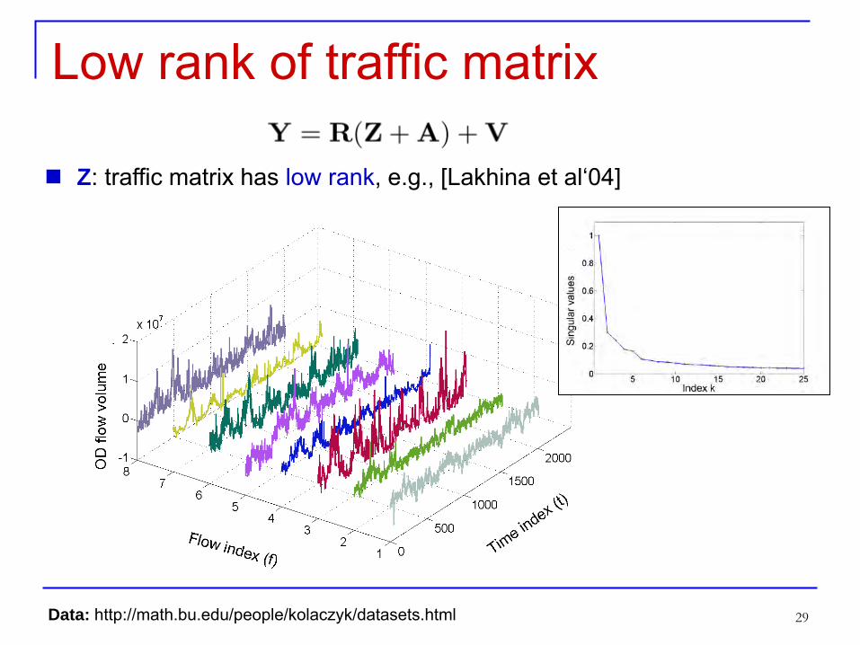
Low rank of traffic matrix

Z: traffic matrix has low rank, e.g., [Lakhina et al‘04]

Data: http://math.bu.edu/people/kolaczyk/datasets.html

30

Sparsity of anomaly matrix

A: anomaly matrix is sparse across both time and flows

0 200 400 600 800 10000

2

4x 108

Time index(t)

|af,t

|

0 50 1000

2

4x 108

Flow index(f)

|af,t

|

Time

Flows

31

Problem statement

Given and routing matrix , identify sparse when is low rank

fat but still low rank

(P1)

Low-rank sparse vector of SVs nuclear norm and norm

32

Anomaly identification Change detection on per-link time series [Brutlag’00], [Casas et al’10] Spatial PCA [Lakhina et al’04] Network anomography [Zhang et al’05]

Prior art

Rank minimization with the nuclear norm, e.g., [Recht-Fazel-Parrilo’10]

Matrix decomposition [Candes et al’10], [Chandrasekaran et al’11]

Principal Component Pursuit

(PCP)

Observed Low rank Sparse

33

Challenges and importance

not necessarily sparse and fat PCP not applicable

Important special cases

R = I : matrix decomposition with PCP [Candes et al’10] X = 0 : compressive sampling with basis pursuit [Chen et al’01] X = CLxρW’ρxT and A = 0 : PCA [Pearson 1901] X = 0, R = D unknown: dictionary learning [Olshausen’97]

LT + FT >> LT

X A Y

STRUCTURE

34

Exact recovery Noise-free case

M. Mardani, G. Mateos, and G. B. Giannakis,``Recovery of low-rank plus compressed sparse matrices with application to unveiling traffic anomalies," IEEE Trans. Information Theory, 2013.

(P0)

Theorem: Given and , assume every row and column of has at most k<s non-zero entries, and has full row rank. If C1)-C2) hold, then with (P0) exactly recovers

C1)

C2)

Q: Can one recover sparse and low-rank exactly? A: Yes! Under certain conditions on

35

Intuition

Exact recovery conditions satisfied if

r and s are sufficiently small

Nonzero entries of A0 are “sufficiently spread out”

Incoherent rank and sparsity- preserving subspaces

R satisfies a restricted isometry property

Remarks Amplitude of non-zero entries of A0 irrelevant Conditions satisfied for certain random ensembles w.h.p.

36

Numerical validation Setup L=105, F=210, T = 420 R ~ Bernoulli(1/2) Xo = RPQ’, P, Q ~ N(0, 1/FT) aij ϵ {-1,0,1} w.p. {π/2, 1-π, π/2}

Relative recovery error

% non-zero entries (ρ)

rank

(XR

) (r)

0.1 2.5 4.5 6.5 8.5 10.5 12.5

10

20

30

40

50

0

0.1

0.2

0.3

0.4

0.5

0.6

0.7

rank

(X0)

[r]

[(s/FT)%]

37

In-network processing Spatially-distributed link count data

Goal: Given local link counts per agent, unveil anomalies in a distributed fashion by leveraging low-rank of the nominal data matrix and sparsity of the outliers.

Challenge: not separable across rows (links/agents)

n

Centralized: Decentralized:

Agent 1

Agent N

Local processing and single-hop communications

38

Separable regularization Key property

Lxρ ≥rank[X]

V’

W’ C

Separable formulation equivalent to (P1)

(P2)

Nonconvex; less variables:

Proposition 3: If stat. pt. of (P2) and , then is a global optimum of (P1).

39

Distributed algorithm

M. Mardani, G. Mateos, and G. B. Giannakis, “In-network sparsity regularized rank minimization: Algorithms and applications," IEEE Transactions on Signal Processing, 2013.

Alternating-direction method of multipliers (ADMM) solver for (P2) Method [Glowinski-Marrocco’75], [Gabay-Mercier’76] Learning over networks [Schizas-Ribeiro-Giannakis’07]

Consensus-based optimization Attains centralized performance

40

Benchmark: PCA-based methods Idea: anomalies increase considerably rank(Y)

Algorithm i) Form subspace via r-dominant left singular vectors of Y (resp. )

Assumes knowledge of r:=rank(X)

σi(X)

Index i

-----Y -----X

ii) Infer anomalies from

[Lakhina et al’04] For t = 1,…,T [Zhang et al’05] Sparse anomalies

41

Synthetic data Random network topology

N=20, L=108, F=360, T=760 Minimum hop-count routing

0 0.2 0.4 0.6 0.8 10

0.2

0.4

0.6

0.8

1

False alarm probability

Det

ectio

n pr

obab

ility

PCA-based method, r=5PCA-based method, r=7PCA-based method, r=9Proposed method, per time and flow

0 0.2 0.4 0.6 0.8 1

0

0.2

0.4

0.6

0.8

1

---- True ---- Estimated

Pf=10-4

Pd = 0.97

42

Internet2 data Real network data

Dec. 8-28, 2008 N=11, L=41, F=121, T=504

0 0.2 0.4 0.6 0.8 10

0.2

0.4

0.6

0.8

1

False alarm probability

Det

ectio

n pr

obab

ility

[Lakhina04], rank=1[Lakhina04], rank=2[Lakhina04], rank=3Proposed method[Zhang05], rank=1[Zhang05], rank=2[Zhang05], rank=3

Data: http://www.cs.bu.edu/~crovella/links.html

0100

200300

400500

0

50

100

0

1

2

3

4

5

6

Time

Pfa = 0.03 Pd = 0.92

---- True ---- Estimated

Flows

Ano

mal

y vo

lum

e

43

Dynamic anomalography

M. Mardani, G. Mateos, and G. B. Giannakis, "Dynamic anomalography: Tracking network anomalies via sparsity and low rank," IEEE Journal of Selected Topics in Signal Processing, pp. 50-66, Feb. 2013.

Construct an estimated map of anomalies in real time

Streaming data model:

(Robust) subspace tracking Projection approximation (PAST) [Yang’95] Missing data: GROUSE [Balzano et al’10], PETRELS [Chi et al’12] Outliers: [Mateos-Giannakis’10], GRASTA [He et al’11]

Compressed “outliers” challenge identifiability

Goal: Given estimate online when is in a low-dimensional space and is sparse

0

2

4CHIN--ATLA

0

20

40

Anom

aly am

plitu

de

WASH--STTL

0 1000 2000 3000 4000 5000 60000

10

20

30

Time index (t)

WASH--WASH

0

5ATLA--HSTN

0

10

20

Link

traff

ic lev

el DNVR--KSCY

0

10

20

Time index (t)

HSTN--ATLA

44

Online estimator Challenge: not separable across columns (time)

Approach: regularized exponentially-weighted LS formulation

---- estimated ---- real

o---- estimated ---- real

45

Delay cartography

Internet2 data (Aug 18-22,2011) End-to-end latency matrix N=9, L=T=N; 20% missing data

Network distance prediction [Liau et al’12]

Data: http://internet2.edu/observatory/archive/data-collections.html

Relative error: 10%

Approach: distributed low-rank matrix completion

Unveiling network traffic anomalies via convex optimization Leveraging sparsity and low rank

46

Takeaways

Reveal when and where anomalies occur

Exact recovery of low-rank plus compressed sparse matrices

Distributed/online algorithms with guaranteed performance

Dynamic network delay cartography

Unveiling network anomalies via sparsity and low rank

Network-wide link count prediction Semi-supervised learning for traffic maps Batch and online processing Empirical validation: Internet2 data

RF cartography for cognition at the PHY Conclusions and future research directions

47

Roadmap

48

A commuting conundrum Objective: map a “good” route for packet delivery

Application domains Transportation networks [Gastner-Newman’04] Communication networks [Soule et al’05] Sensor networks [Abrams et al’04]

Measure traffic at few roads/links only

49

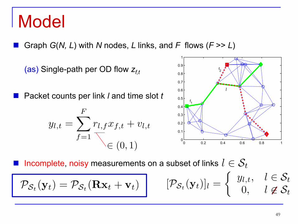
Model Graph G(N, L) with N nodes, L links, and F flows (F >> L) (as) Single-path per OD flow zf,t Packet counts per link l and time slot t

Incomplete, noisy measurements on a subset of links

0 0.2 0.4 0.6 0.8 10

0.1

0.2

0.3

0.4

0.5

0.6

0.7

0.8

0.9

1

f1

f2

l

50

Problem statement

Goal: Given and historical data , find

Impact Ability to handle missing data Online prediction capturing spatio-temporal correlations Computationally-efficient link traffic prediction

P. A. Forero, K. Rajawat, and G. B. Giannakis, “Prediction of partially observed dynamical processes over networks via dictionary learning,” J. Machine Learning Research, 2013.

Prior art Traffic estimation [Zhang et al’05] Kriging [Chua et al’06], plus traffic modeling [Vaughn et al’10] Topology-driven basis expansion [Crovella-Kolaczyk’03], [Coates et al’07]

51

Data-driven model of link counts Sparse representation of link counts

Notation:

Dictionary Learning (DL) [Olshausen-Field’97] Given , find dictionary (basis) and sparse

Q: How about DL from incomplete data ?

52

Capturing spatial link dependence Auxiliary graph with vertices = links in G Edge weights = number of OD flows common to links Adjacency matrix: , graph Laplacian

1 1

1 1

1

G

Regularizers effect sparsity and smoothness over

Cost function to learn D

53

Semi-supervised DL Semi-supervised Dictionary Learning (SSDL)

Given , find dictionary (basis) and sparse

SSDL biconvex, block-coordinate descent (BCD) solver Update via parallel entry-wise soft-thresholding Update each via QP + projection onto the Euclidean ball

Proposition: BCD’s iterates converge to a stationary point of SSDL

γ -γ

54

Link load prediction Given and learnt dictionary , solve

Captures sparsity of and smoothness of link loads over

Predict based on

Scaling factor reduces bias in [Zou-Hastie’05]

55

Batch processing summary

56

Test case: Internet2 Internet2 measurement archive

Prediction improves as link load increases

Training phase – 30 links measured Operational phase – 30 links measured

L=54, T=2000

57

Prediction error (Internet2) Normalized prediction error:

Q = number of columns of D; t0=2000

Gravity-based [Zhang et al’05]; Diffusion wavelets [Coifman-Maggioni’07]

SSDL outperforms competing alternatives

Training with 30 links Training with 50 links

58

Online processing Capture temporal correlations on

Given and dictionary , solve

Predict based on

Dictionary update

59

Real-time prediction (Internet2) Q=60, different values of the forgetting factor Measure traffic at 30 links only

SSDL-based tracker outperforms diffusion wavelets

Prediction of network processes from incomplete observations

60

Takeaways

Spatial correlation of link counts via Laplacian regularization

Online algorithms capturing temporal correlations

Semi-supervised learning

Link count prediction based on dictionary learning

Dynamic network delay cartography

Unveiling network anomalies via sparsity and low rank

Network-wide link count prediction RF cartography for cognition at the PHY Interference spectrum cartography Channel gain cartography

Conclusions and future research directions

61

Roadmap

62

Fixed radio Policy-based: parameters set by

operators

Software-defined radio (SDR) Programmable: can adjust

parameters to intended link

Cognitive radio (CR) Intelligent: sense the environment

& learn to adapt [Mitola’00]

RX

TX

CR

Dynamic Resource Allocation

RF environment

- sensing - learning

- adapting to spectrum

What is a cognitive radio?

Cognizant transceiver: sensing Agile transmitter: adaptation Intelligent DRA: decision making Radio reconfiguration decisions Spectrum access decisions

63

US FCC

Inefficient occupancy

0 1 2 3 4 5 6GHz

PS

D

Spectrum scarcity problem

Fixed spectrum access policies Useful radio spectrum pre-assigned

64

PSD

f

SU

PU1

PU2 PU3

noise floor

PSD

f

SU PU1

PU2

PU3

Dynamical access under user hierarchy

Spectrum underlay Restriction on transmit power levels Operation over ultra wide bandwidths

Spectrum overlay Constraints on when and where to transmit Avoid interference to Pus via sensing and adaptive allocation

Primary users (PUs) versus secondary users (SUs/CRs)

Spectrum underlay Spectrum overlay

65

Source: Office of Communications (UK)

Cooperative sensing for efficient sharing Multiple CRs jointly detect the spectrum [Ganesan-Li’06][Ghasemi-Sousa’07]

Benefits of cooperation Spatial diversity gain mitigates multipath fading/shadowing Reduced sensing time and local processing Ability to cope with hidden terminal problem

Limitation: existing approaches do not exploit space-time dimensions

66 J. A. Bazerque and G. B. Giannakis, “Distributed spectrum sensing for cognitive radio networks by exploiting sparsity,'’ IEEE Transactions on Signal Processing, pp. 1847-1862, March 2010.

Cooperative PSD cartography Idea: CRs collaborate to form a spatial map of the RF spectrum

Goal: Find PSD map across space and frequency

Specifications: coarse approx. suffices

Approach: basis expansion of

67

Modeling Transmitters

Sensing CRs

Frequency bases

Sensed frequencies

Sparsity present in space and frequency

Data Rx-power at cognitive radio

Space-frequency basis expansion Find Tx-power of source s over frequency band

68

Estimate sparse to find PSD at

Sparsity-promoting regularization

69

Exchange of local estimates

Scalability

Robustness Lack of infrastructure

Decentralized Ad-hoc

Centralized Fusion

center

Distributed recursive implementation

Consensus-based approach Solve locally

Constrained optimization using ADMM

RF spectrum cartography sources

70

NNLS Lasso

As a byproduct, Lasso localizes all sources via variable selection

candidate locations, CRs

71

Centralized sensing No fading Ns=25

4 CR Rxs

2 CR Txs

Simulated test: PSD map estimation

72

“True” Tx spectrum

Sensed at the consensus step

Distributed consensus with fading

Starting from a local estimate, sensors reach consensus

73 J. A. Bazerque, G. Mateos, and G. B. Giannakis, ``Group-Lasso on Splines for Spectrum Cartography,’’ IEEE Transactions on Signal Processing,’’ pp. 4648-4663, October 2011.

Spline-based PSD cartography Q: How about shadowing?

: unknown dependence on spatial variable x

Path-loss Shadowing

A: Basis expansion with coefficient functions

74

Frequency basis expansion PSD of Tx source is

Basis expansion in frequency

Basis functions Accommodate prior knowledge raised-cosine Sharp transitions (regulatory masks) rectangular, non-overlapping Overcomplete basis set (large ) robustness

75

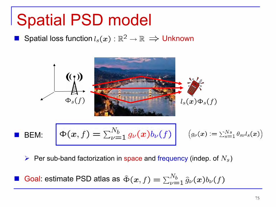
Spatial PSD model Spatial loss function Unknown

Per sub-band factorization in space and frequency (indep. of )

BEM:

Goal: estimate PSD atlas as

Nonparametric basis pursuit

Twofold regularization of variational LS estimator

(P1)

Available data: location of CRs measured frequencies

Observations

76

Avoid overfitting by promoting smoothness

Nonparametric basis selection ( not selected)

77

Thin-plate splines solution

Unique, closed-form, finitely-parameterized minimizers!

Proposition 1: Estimates in (P1) are thin-plate splines [Duchon’77]

where is the radial basis function , and

Q2: How does (P1) perform basis selection?

Q1: How to estimate based on ?

78

Lassoing bases (P1) equivalent to group Lasso estimator [Yuan-Lin’06]

Matrices ( and dependent)

i) ii) iii)

Group Lasso encourages sparse factors Full-rank mapping:

Proposition 2:

as

w/

Minimizers of (P1) are fully determined by

79

Simulated test

S P E C T R U M M A P

Basis index Frequency (Mhz)

sources; raised cosine pulses sensing CRs, sampling frequencies bases; (roll off x center frequency x bandwidth)

Original Estimated

80

Numerical test IEEE 802.11 PUs

PSD cartography

Maps estimated under fading + shadowing + overlapping bases

CRs

Original Estimated

Channel 6

Channel 11

81

Real RF data

Frequency bases identified Maps recovered and extrapolated

IEEE 802.11 WLAN activity sensed

CRs

1

2

3

4

5

6

7

8

9

10

11

12

13

14

-50 -60 -40 -30 -20 -10 (dBi)

82

Semi-supervised DL for PSD maps

S.-J. Kim and G. B. Giannakis, "Cognitive Radio Spectrum Prediction using Dictionary Learning," Proc. of Globecom Conf., Atlanta, GA, 2013.

Signal model

Rx-power measured by a few CRs

Batch formulation

Online algorithm via exponentially weighted criterion

83

Numerical tests

84

Recap: PHY sensing via RF cartography

S.-J. Kim, E. Dall’Anese, and G. B. Giannakis,“Cooperative Spectrum Sensing for Cognitive Radios using Kriged Kalman Filtering,” IEEE J. Selected Topics in Signal Processing, pp. 24-36, Feb. 2011.

Power spectral density (PSD) maps

Capture ambient power in space-time-frequency

Can identify “crowded” regions to be avoided

Channel gain (CG) maps

Time-frequency channel from any-to-any point

CRs adjust Tx power to min. PU disruption

E. Dall’Anese, S.-J. Kim, and G. B. Giannakis, “Channel Gain Map Tracking via Distributed Kriging,” IEEE Trans. on Vehicular Technology, pp. 1205-1211, March 2011. 85

Kalman filtering

Kriging interpolation

Approach: spatial LMMSE interpolation (Kriging) + KF for tracking channel dynamics

Payoffs: tracking PU activities; accurate interference models; efficient resource allocation

Outlook: jointly optimal PHY CR sensing and access

Channel gain cartography CG after averaging small-scale fading (dB)

State-space model for shadowing

86

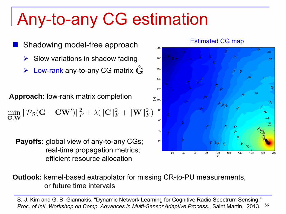
Approach: low-rank matrix completion

Payoffs: global view of any-to-any CGs; real-time propagation metrics; efficient resource allocation

Outlook: kernel-based extrapolator for missing CR-to-PU measurements, or future time intervals

Any-to-any CG estimation Shadowing model-free approach

Slow variations in shadow fading

Low-rank any-to-any CG matrix

Estimated CG map

S.-J. Kim and G. B. Giannakis, “Dynamic Network Learning for Cognitive Radio Spectrum Sensing,” Proc. of Intl. Workshop on Comp. Advances in Multi-Sensor Adaptive Process., Saint Martin, 2013.

87

Approach: blind dictionary learning

Payoffs: tracking PU activities; efficient resource allocation

Outlook: missing data due to limited sensing; distributed and robust algorithms

PU power and CR-PU link learning Reduce overhead in any-to-any CG mapping

Learn CGs only between CRs and PUs

Detection of PU activity

Estimated CG

Online detection of active PU transmitters

S.-J. Kim, N. Jain, and G. B. Giannakis, “Joint Link Learning and Cognitive Radio Sensing," in Proc. of Asilomar Conf. on Signals, Systems, and Computers, Pacific Grove, CA, Nov. 2011.

88

Takeaways PHY layer spatiotemporal sensing via RF cartography Space-time-frequency view of interference and channel gains

PU/source localization and tracking

Parsimony via sparsity and distribution via consensus Lasso, group Lasso on splines, and method of multipliers

Identify idle bands across space Aid dynamic spectrum access policies

Dynamic network delay cartography

Unveiling network anomalies via sparsity and low rank

Network-wide link count prediction RF cartography for cognition at the PHY Conclusions and future research directions

89

Roadmap

90

The big picture ahead… Network path delay maps

0100

200300

400500

0

50

100

0

1

2

3

4

5

6

Time

Network traffic anomaly maps

Flows

Ano

mal

y vo

lum

e

RF interference cartography

Channel gain maps Coverage maps

Network cartography: succinct depiction of the network state

Vision: use atlas to enable spatial re-use, hand-off, localization, Tx-power tracking, resource allocation, health monitoring, and routing

91

Concluding summary Dynamic network cartography

Global state mapping from incomplete and corrupted data

Statistical SP toolbox Sparsity-cognizant learning, low-rank modeling

Framework to construct maps of the dynamic network state Real-time, distributed scalable algorithms for large-scale networks

Path delay and link traffic maps Prompt and accurate identification of traffic anomalies PHY layer sensing in wireless CR networks via RF cartography

Kriged Kalman filtering of dynamical processes over networks Semi-supervised dictionary learning Distributed optimization via the ADMM Thank you!

92

Questions?

http://spincom.umn.edu University of Minnesota

Dr. J. A. Bazerque UofM

Dr. E. Dall’Anese UofM

Dr. P. A. Forero SPAWAR

Dr. S. J. Kim UofM

M. Mardani UofM

Prof. K. Rajawat IIT Kanpur