Carry Trade and Momentum in Currency Markets

April 2011

Craig BurnsideDuke University and NBERburnside@econ.duke.edu

Martin EichenbaumNorthwestern University, NBER, and Federal Reserve Bank of Chicagoeich@northwestern.edu

Sergio RebeloNorthwestern University, NBER, and CEPR.s-rebelo@kellogg.northwestern.edu

Corresponding author: Sergio Rebelo, Kellogg School of Management, Northwestern Uni-versity, Evanston IL 60208, USA

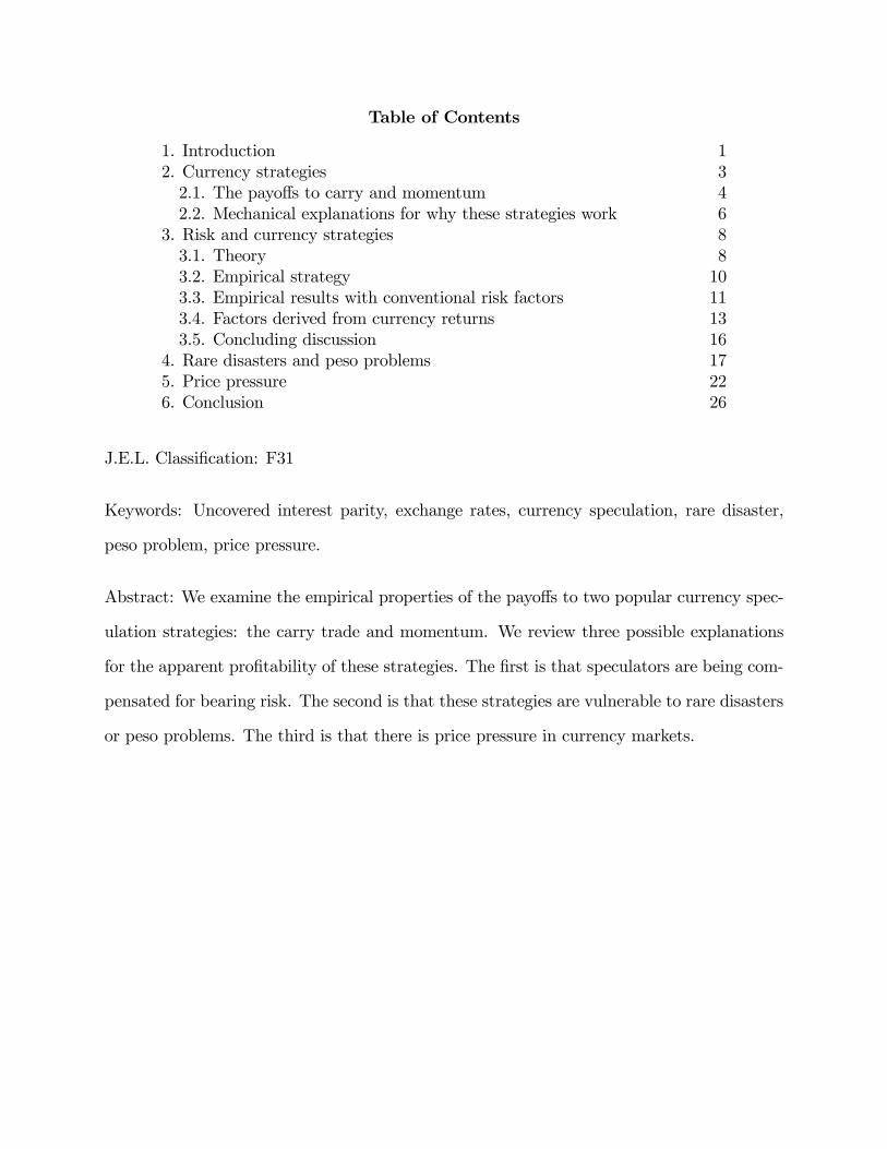
Table of Contents

1. Introduction 12. Currency strategies 32.1. The payo!s to carry and momentum 42.2. Mechanical explanations for why these strategies work 6

3. Risk and currency strategies 83.1. Theory 83.2. Empirical strategy 103.3. Empirical results with conventional risk factors 113.4. Factors derived from currency returns 133.5. Concluding discussion 16

4. Rare disasters and peso problems 175. Price pressure 226. Conclusion 26

J.E.L. Classification: F31

Keywords: Uncovered interest parity, exchange rates, currency speculation, rare disaster,

peso problem, price pressure.

Abstract: We examine the empirical properties of the payo!s to two popular currency spec-

ulation strategies: the carry trade and momentum. We review three possible explanations

for the apparent profitability of these strategies. The first is that speculators are being com-

pensated for bearing risk. The second is that these strategies are vulnerable to rare disasters

or peso problems. The third is that there is price pressure in currency markets.

1 Introduction

In this survey we examine the empirical properties of the payo!s to two currency speculation

strategies: the carry trade and momentum. We then assess the plausibility of the theories

proposed in the literature to explain the profitability of these strategies.

The carry trade consists of borrowing low-interest-rate currencies and lending high-

interest-rate currencies. The momentum strategy consists of going long (short) on currencies

for which long positions have yielded positive (negative) returns in the recent past.

The carry trade, one of the oldest and most popular currency speculation strategies, is

motivated by the failure of uncovered interest parity (UIP) documented by Bilson (1981)

and Fama (1984).1 This strategy has received a great deal of attention in the academic

literature as researchers struggle to explain its apparent profitability. Papers that study this

strategy include Lustig & Verdelhan (2007), Brunnermeier et al. (2009), Jordà & Taylor

(2009), Farhi et al. (2009), Lustig et al. (2009), Ra!erty (2010), Burnside et al. (2011), and

Menkho! et al. (2011a).

In related work, a number of authors have studied the properties of currency momentum

strategies. These authors include Okunev and White (2003), Lustig et al. (2009), Menkho!

et al. (2011a, 2011b), Moskowitz et al. (2010), Ra!erty (2010), and Asness et al. (2009).

We begin by addressing the question: is the profitability of the carry trade and momentum

strategies just compensation for risk, at least as conventionally measured? After reviewing

the empirical evidence we conclude that the answer is no. This conclusion rests on the fact

that the covariance between the payo!s to these two strategies and conventional risk factors

is not statistically significant.2

The di"culty in explaining the profitability of the carry trade with conventional risk

factors has led researchers such as Lustig et al. (2009) and Menkho! et al. (2011a) to

1See Hodrick (1987) and Engel (1996) for surveys of the literature on uncovered interest parity.2This finding is consistent with work documenting that one can reject consumption-based asset pricing

models using data on forward exchange rates. See, e.g. Bekaert and Hodrick (1992) and Backus, Foresi, andTelmer (2001)).

1

construct empirical risk factors specifically designed to price the average payo!s to portfolios

of carry trade strategies. One natural question is whether these risk factors explain the

profitability of the momentum strategy. We find that they do not.

An alternative explanation for the profitability of our two strategies is that it reflects the

presence of rare disasters or peso problem explanations. We argue, on empirical grounds,

that the 2008 financial crisis cannot be used as an example of the kind of rare disaster that

rationalizes the profitability of currency trading. The reason is simple: momentum made

money during the financial crisis.

We then consider the literature that uses currency options data to characterize the nature

of the peso event that rationalizes the profitability of carry and momentum. Based on this

analysis we argue that the peso event features moderate losses but a high value of the

stochastic discount factor (SDF).

Finally, we explore an alternative explanation for the profitability of the carry trade and

momentum strategies. This alternative relies on the existence of price pressure in foreign

exchange markets. By price pressure we mean that the price at which investors can buy or sell

currencies depends on the quantity they wish to transact. Price pressure introduces a wedge

between marginal and average payo!s to a trading strategy. As a result, observed average

payo!s can be positive even though the marginal trade is not profitable. So, traders do not

increase their exposure to the strategy to the point where observed average risk-adjusted

payo!s are zero.

The paper is organized as follows. In Section 2 we describe the empirical properties of

the payo!s to the two currency strategies that we consider. In Section 3 we discuss risk-

based explanations for the profitability of these strategies. Section 4 discusses the impact

on inference that results from rare disasters or peso problems. Section 5 provides a brief

discussion of the implications of price pressure. A final section concludes.

2

2 Currency strategies

In this section we describe the carry trade and currency momentum strategies.

The carry trade strategy This strategy consists of borrowing low-interest-rate currencies

and lending high-interest-rate currencies. Assume that the domestic currency is the U.S.

dollar (USD) and denote the USD risk-free rate by it. Let the interest rate on risk-free

foreign denominated securities be i!t . Abstracting from transactions costs, the payo! to

taking a long position on foreign currency is:

zLt+1 = (1 + i!t )St+1St

! (1 + it) . (1)

Here St denotes the spot exchange rate expressed as USD per foreign currency unit (FCU).

The payo! to the carry trade strategy is:

zCt+1 = sign(i!t ! it)z

Lt+1. (2)

An alternative way to implement the carry trade is to use forward contracts. We denote

by Ft the time-t forward exchange rate for contracts that mature at time t + 1, expressed

as USD per FCU. A currency is said to be at a forward premium relative to the USD if Ft

exceeds St. The carry trade can be implemented by selling forward currencies that are at a

forward premium and buying forward currencies that are at a forward discount. The time t

payo! to this strategy can be written as:

zFt+1 = sign(Ft ! St)(Ft ! St+1). (3)

It is easy to show that, when covered interest parity (CIP) holds, these two ways of

implementing the carry trade are equivalent in the sense that zCt+1 and zFt+1 are proportional.

3

So, whenever one strategy makes positive profits so does the other.

3Taking transactions costs into account, deviations from CIP are generally small and rare. See Taylor(1987, 1989), Clinton (1988), and Burnside, Eichenbaum, Kleschelski and Rebelo (2006). However, therewere significant deviations from CIP in the aftermath of the 2008 financial crisis. These deviations are likelyto have resulted from liquidity issues and counterparty risk. See Mancini-Gri!oli and Ranaldo (2011) for adiscussion.

3

The portfolio carry trade strategy that we consider combines all the individual carry

trades in an equally-weighted portfolio. The total value of the bet is normalized to one USD.

We refer to this strategy as the “carry trade portfolio.” It is the same as the equally-weighted

strategy studied by Burnside et al. (2011).

The momentum strategy This strategy involves selling (buying) a FCU forward if it

was profitable to sell (buy) a FCU forward at time t ! ! . Following Lustig et al. (2009),

Menkho! et al. (2011a), Moskowitz et al. (2010), and Ra!erty (2010), we define momentum

in terms of the previous month’s return, i.e. we choose ! = 1. The excess return to the

momentum strategy is:

zMt+1 = sign(zLt )z

Lt+1. (4)

We consider momentum trades conducted one currency at a time against the U.S. dollar.

We also consider a portfolio momentum strategy that combines all the individual momentum

trades in an equally-weighted portfolio with the total value of the bet being normalized to

one USD. We refer to this strategy as the “momentum portfolio.”4

2.1 The payo!s to carry and momentum

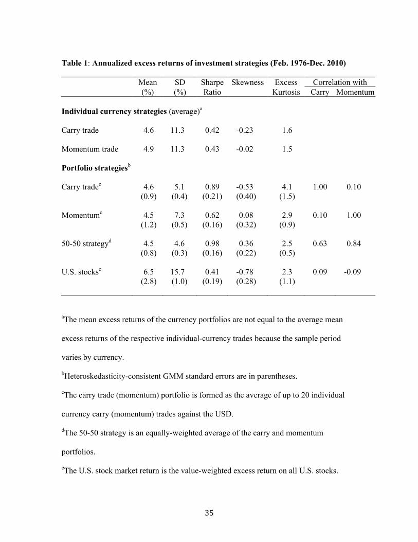
Table 1 provides summary statistics for the payo!s to our two currency strategies imple-

mented for 20 major currencies, over the sample period 1976-2010.5 In every case, the size

of the bet is normalized to one USD.

The carry trade strategy Consider, first, the equally-weighted carry trade strategy. This

strategy has an average payo! of 4.6 percent, with a standard deviation of 5.1 percent, and

a Sharpe ratio of 0.89. In comparison, the average excess return to the U.S. stock market

4The strategy we consider di!ers from some momentum strategies studied in the literature, which consistof going long (short) on assets that have done relatively well (poorly) in the recent past, even if the returnto these assets was negative (positive). See Jegadeesh & Titman (1993), Carhart (1997), and Rouwenhorst(1998) for a discussion of this cross-sectional momentum strategy in equity markets.

5See Burnside et al. (2011) for a description of our data sources.

4

over the same period is 6.5 percent, with a standard deviation of 15.7 percent and a Sharpe

ratio of 0.41.

Consider, next, the average payo! to the individual carry trades. Averaged across the

20 currencies, this payo! is 4.6 percent with an average standard deviation of 11.3 percent.6

The corresponding Sharpe ratio is 0.42. The Sharpe ratio of the equally-weighted carry trade

is more than twice as large. Consistent with Burnside et al. (2007, 2008), this di!erence is

entirely attributable to the gains of diversifying across currencies, which cuts volatility by

more than 50 percent.

The momentum strategy The equally-weighted momentum strategy is also highly prof-

itable, yielding an average payo! of 4.5 percent. These payo!s have a standard deviation of

7.3 percent and a Sharpe ratio of 0.62. Again, there are substantial returns to diversifying

across individual momentum strategies. The average payo! of individual momentum strate-

gies across the 20 currencies is equal to 4.9 percent. The corresponding average standard

deviation is 11.3 percent and the Sharpe ratio is 0.43. An equally-weighted combination of

the two currency strategies, which we call the “50-50 strategy”, has an average payo! of 4.5

percent, a standard deviation of 4.6 percent and a Sharpe ratio of 0.98. The high Sharpe

ratio of the combined strategy reflects the low correlation between the payo!s to the two

strategies.

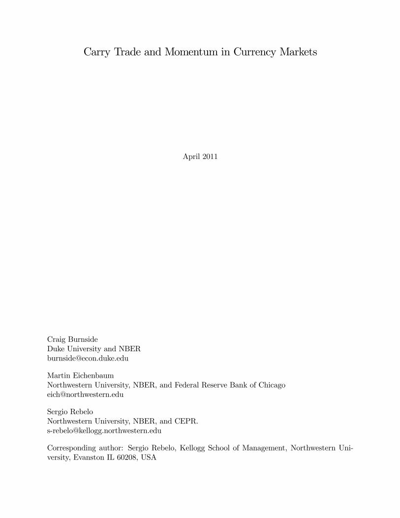
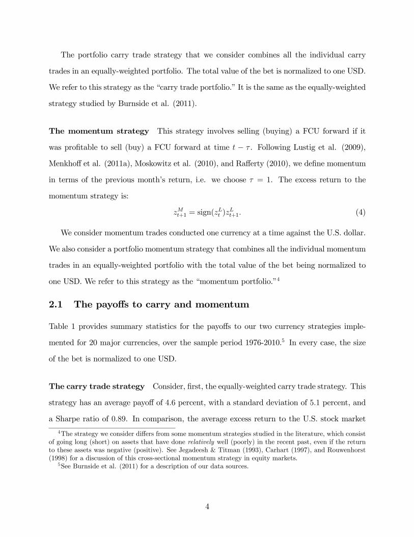
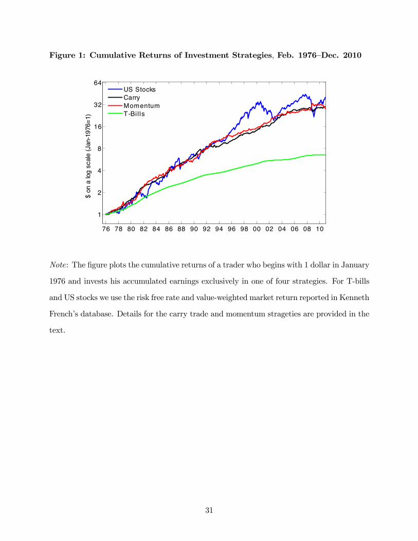
Figure 1 displays the cumulative returns to investing in the carry and momentum port-

folios, in the U.S. stock market, and in Treasury bills. Since the currency strategies involve

zero net investment we compute the cumulative payo!s as follows. We initially deposit one

USD in a bank account that yields the same rate of return as the Treasury bill rate. In

the beginning of every period we bet the balance of the bank account on the strategy. At

the end of the period, payo!s to the strategy are deposited into the bank account. Figure

1 shows that the cumulative returns to the carry and momentum portfolios are almost as

6The average payo! across individual carry trades does not (to two digits) coincide with the averagepayo! to the equally-weighted portfolio because not all currencies are available for the full sample.

5

high as the cumulative return to investing in stocks. By the end of the sample the carry

trade, momentum, and stock portfolios are worth $30.09, $27.98, and $40.22, respectively.

However, the cumulative returns to the stock market are much more volatile than those of

the currency portfolios. Also, note that most of the returns to holding stocks occur prior

to the year 2000. An investor holding the market portfolio from the end of August 2000

until December 2010 earned a cumulative return of only 14.9 percent. Investors in risk-free

assets, carry, and momentum earned cumulative returns of 26.7 percent, 93.9 percent, and

76.1 percent, respectively, over the same period.

The payo!s to currency strategies are often characterized as being highly skewed (see

e.g. Brunnermeier et al., 2009). Our point estimates indicate that carry trade payo!s are

skewed, but this skewness is not statistically significant. Interestingly, carry trade payo!s

are less skewed than the payo!s to the U.S. stock market. The payo!s to the momentum

portfolio are actually positively skewed, though not significantly so.

As far as fat tails are concerned, currency returns display excess kurtosis, with noticeable

central peakedness, especially in the case of the carry trade portfolio. It is not obvious, how-

ever, that investors would be deterred by this kurtosis, given the relatively small variance of

carry trade payo!s, when compared to that of the aggregate stock market. Indeed, Burnside

et al. (2006) use a simple portfolio allocation model to show that a hypothetical investor

with constant relative risk aversion preferences, and a risk aversion coe"cient of five, would

allocate three times as much of his portfolio to diversified carry trades as he would to U.S.

stocks.

2.2 Mechanical explanations for why these strategies work

In this section, we relate the observed profitability of the carry trade and momentum strate-

gies to the empirical failure of UIP. The payo!s to the strategies can each be written as:

zt+1 = utzLt+1. (5)

The two strategies di!er only in the definition of ut.

6

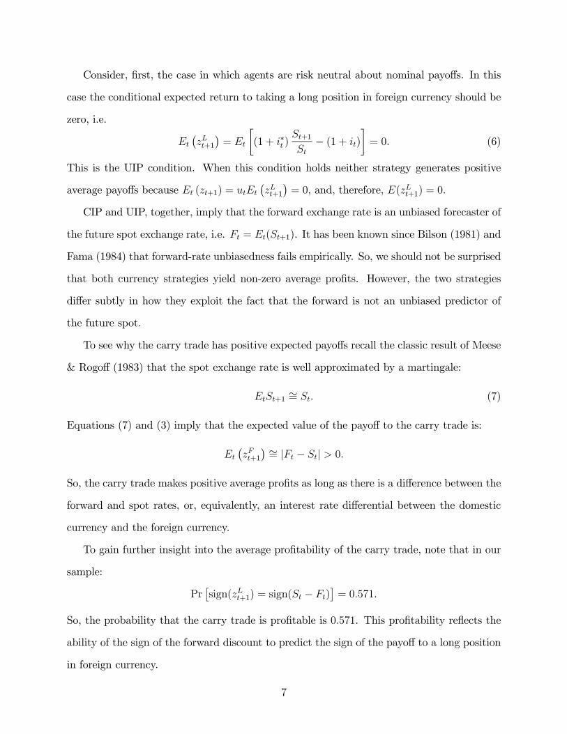
Consider, first, the case in which agents are risk neutral about nominal payo!s. In this

case the conditional expected return to taking a long position in foreign currency should be

zero, i.e.

Et!zLt+1

"= Et

#(1 + i!t )

St+1St

! (1 + it)$= 0. (6)

This is the UIP condition. When this condition holds neither strategy generates positive

average payo!s because Et (zt+1) = utEt!zLt+1

"= 0, and, therefore, E(zLt+1) = 0.

CIP and UIP, together, imply that the forward exchange rate is an unbiased forecaster of

the future spot exchange rate, i.e. Ft = Et(St+1). It has been known since Bilson (1981) and

Fama (1984) that forward-rate unbiasedness fails empirically. So, we should not be surprised

that both currency strategies yield non-zero average profits. However, the two strategies

di!er subtly in how they exploit the fact that the forward is not an unbiased predictor of

the future spot.

To see why the carry trade has positive expected payo!s recall the classic result of Meese

& Rogo! (1983) that the spot exchange rate is well approximated by a martingale:

EtSt+1 "= St. (7)

Equations (7) and (3) imply that the expected value of the payo! to the carry trade is:

Et!zFt+1

" "= |Ft ! St| > 0.

So, the carry trade makes positive average profits as long as there is a di!erence between the

forward and spot rates, or, equivalently, an interest rate di!erential between the domestic

currency and the foreign currency.

To gain further insight into the average profitability of the carry trade, note that in our

sample:

Pr%sign(zLt+1) = sign(St ! Ft)

&= 0.571.

So, the probability that the carry trade is profitable is 0.571. This profitability reflects the

ability of the sign of the forward discount to predict the sign of the payo! to a long position

in foreign currency.

7

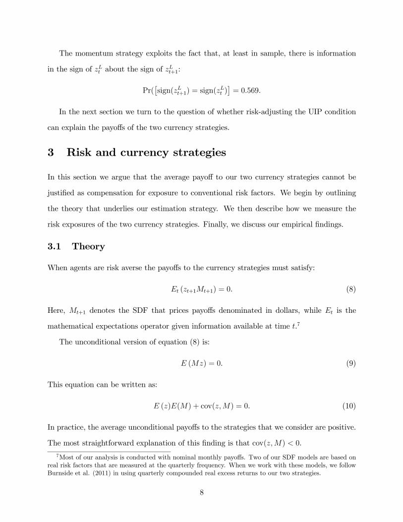
The momentum strategy exploits the fact that, at least in sample, there is information

in the sign of zLt about the sign of zLt+1:

Pr(%sign(zLt+1) = sign(z

Lt )&= 0.569.

In the next section we turn to the question of whether risk-adjusting the UIP condition

can explain the payo!s of the two currency strategies.

3 Risk and currency strategies

In this section we argue that the average payo! to our two currency strategies cannot be

justified as compensation for exposure to conventional risk factors. We begin by outlining

the theory that underlies our estimation strategy. We then describe how we measure the

risk exposures of the two currency strategies. Finally, we discuss our empirical findings.

3.1 Theory

When agents are risk averse the payo!s to the currency strategies must satisfy:

Et (zt+1Mt+1) = 0. (8)

Here, Mt+1 denotes the SDF that prices payo!s denominated in dollars, while Et is the

mathematical expectations operator given information available at time t.7

The unconditional version of equation (8) is:

E (Mz) = 0. (9)

This equation can be written as:

E (z)E(M) + cov(z,M) = 0. (10)

In practice, the average unconditional payo!s to the strategies that we consider are positive.

The most straightforward explanation of this finding is that cov(z,M) < 0.

7Most of our analysis is conducted with nominal monthly payo!s. Two of our SDF models are based onreal risk factors that are measured at the quarterly frequency. When we work with these models, we followBurnside et al. (2011) in using quarterly compounded real excess returns to our two strategies.

8

One can always rationalize the observed payo!s to these strategies by using a statistical

model to compute the risk premium as a residual. Consider, for example, the carry trade,

in which case we can write equation (8) as:

Ft ! St = Et (St+1 ! St) + pt. (11)

Here, pt is the risk premium which is given by:

pt =covt (Mt+1, St+1 ! St)

EtMt+1

.

Given a statistical model for Et (St+1 ! St), we can use equation (11) to back out a time

series for pt and call that residual a “risk premium”:

pt = Ft ! St ! Et (St+1 ! St) .

By construction, this risk premium can rationalize the payo!s to the carry trade. If the spot

exchange rate is a martingale, this procedure amounts to labeling the forward premium the

risk premium. While such an exercise can provide insights, we view the key challenge as

finding observable risk factors that are correlated with the payo!s of the two strategies.

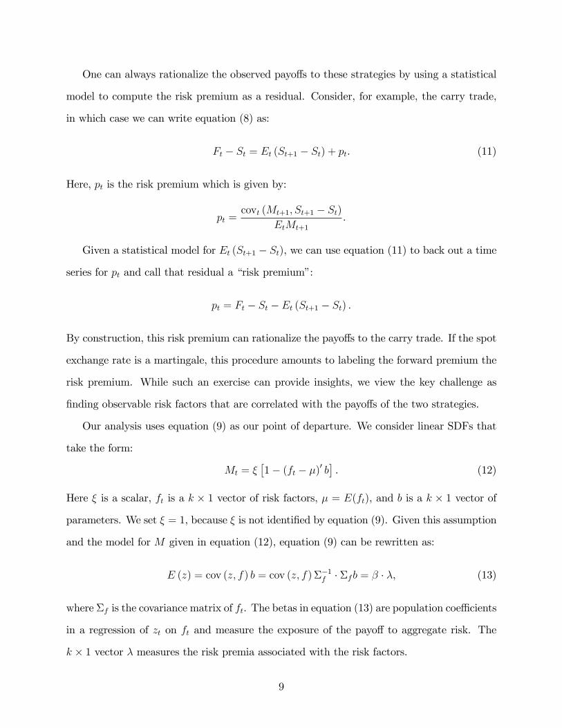
Our analysis uses equation (9) as our point of departure. We consider linear SDFs that

take the form:

Mt = "%1! (ft ! µ)

" b&. (12)

Here " is a scalar, ft is a k # 1 vector of risk factors, µ = E(ft), and b is a k # 1 vector of

parameters. We set " = 1, because " is not identified by equation (9). Given this assumption

and the model for M given in equation (12), equation (9) can be rewritten as:

E (z) = cov (z, f) b = cov (z, f)!#1f · !fb = # · $, (13)

where !f is the covariance matrix of ft. The betas in equation (13) are population coe"cients

in a regression of zt on ft and measure the exposure of the payo! to aggregate risk. The

k # 1 vector $ measures the risk premia associated with the risk factors.

9

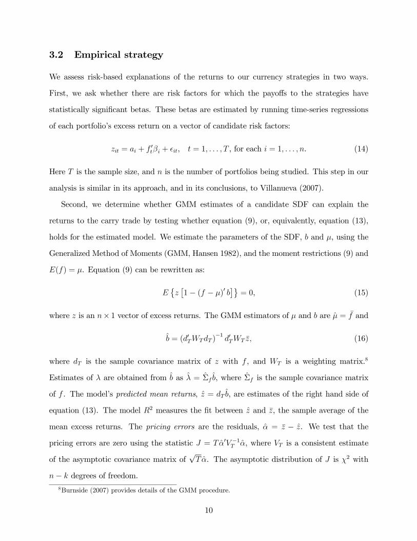
3.2 Empirical strategy

We assess risk-based explanations of the returns to our currency strategies in two ways.

First, we ask whether there are risk factors for which the payo!s to the strategies have

statistically significant betas. These betas are estimated by running time-series regressions

of each portfolio’s excess return on a vector of candidate risk factors:

zit = ai + f"t#i + %it, t = 1, . . . , T , for each i = 1, . . . , n. (14)

Here T is the sample size, and n is the number of portfolios being studied. This step in our

analysis is similar in its approach, and in its conclusions, to Villanueva (2007).

Second, we determine whether GMM estimates of a candidate SDF can explain the

returns to the carry trade by testing whether equation (9), or, equivalently, equation (13),

holds for the estimated model. We estimate the parameters of the SDF, b and µ, using the

Generalized Method of Moments (GMM, Hansen 1982), and the moment restrictions (9) and

E(f) = µ. Equation (9) can be rewritten as:

E'z%1! (f ! µ)" b

&(= 0, (15)

where z is an n# 1 vector of excess returns. The GMM estimators of µ and b are µ = f and

b = (d"TWTdT )#1d"TWT z, (16)

where dT is the sample covariance matrix of z with f , and WT is a weighting matrix.8

Estimates of $ are obtained from b as $ = !f b, where !f is the sample covariance matrix

of f . The model’s predicted mean returns, z = dT b, are estimates of the right hand side of

equation (13). The model R2 measures the fit between z and z, the sample average of the

mean excess returns. The pricing errors are the residuals, & = z ! z. We test that the

pricing errors are zero using the statistic J = T &"V #1T &, where VT is a consistent estimate

of the asymptotic covariance matrix of$T &. The asymptotic distribution of J is '2 with

n! k degrees of freedom.8Burnside (2007) provides details of the GMM procedure.

10

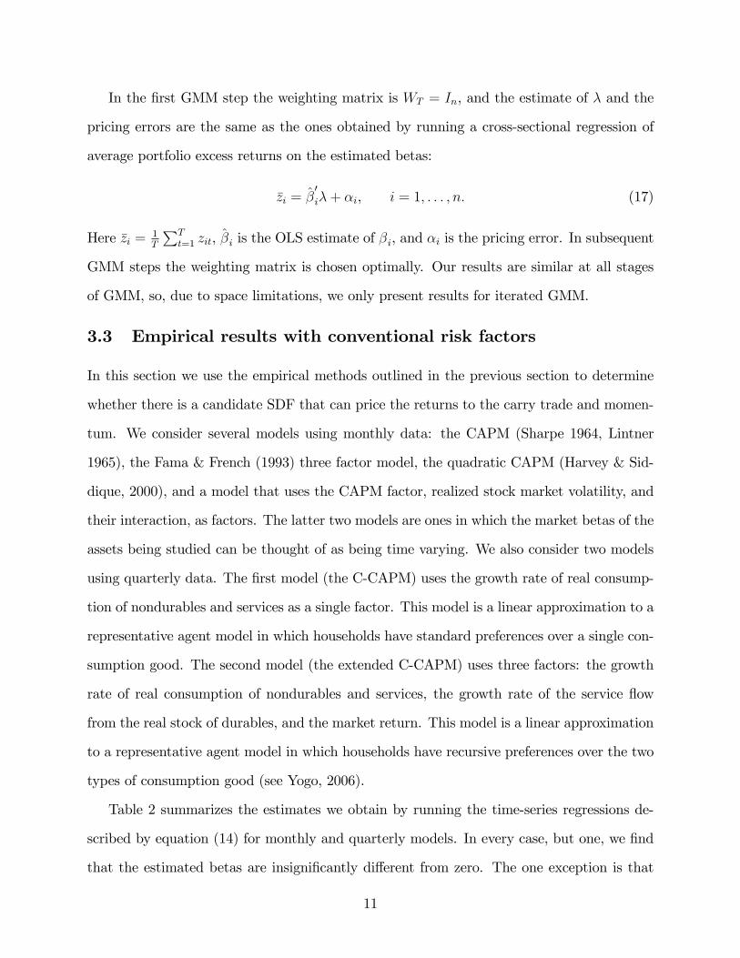
In the first GMM step the weighting matrix is WT = In, and the estimate of $ and the

pricing errors are the same as the ones obtained by running a cross-sectional regression of

average portfolio excess returns on the estimated betas:

zi = #"i$+ &i, i = 1, . . . , n. (17)

Here zi = 1T

)Tt=1 zit, #i is the OLS estimate of #i, and &i is the pricing error. In subsequent

GMM steps the weighting matrix is chosen optimally. Our results are similar at all stages

of GMM, so, due to space limitations, we only present results for iterated GMM.

3.3 Empirical results with conventional risk factors

In this section we use the empirical methods outlined in the previous section to determine

whether there is a candidate SDF that can price the returns to the carry trade and momen-

tum. We consider several models using monthly data: the CAPM (Sharpe 1964, Lintner

1965), the Fama & French (1993) three factor model, the quadratic CAPM (Harvey & Sid-

dique, 2000), and a model that uses the CAPM factor, realized stock market volatility, and

their interaction, as factors. The latter two models are ones in which the market betas of the

assets being studied can be thought of as being time varying. We also consider two models

using quarterly data. The first model (the C-CAPM) uses the growth rate of real consump-

tion of nondurables and services as a single factor. This model is a linear approximation to a

representative agent model in which households have standard preferences over a single con-

sumption good. The second model (the extended C-CAPM) uses three factors: the growth

rate of real consumption of nondurables and services, the growth rate of the service flow

from the real stock of durables, and the market return. This model is a linear approximation

to a representative agent model in which households have recursive preferences over the two

types of consumption good (see Yogo, 2006).

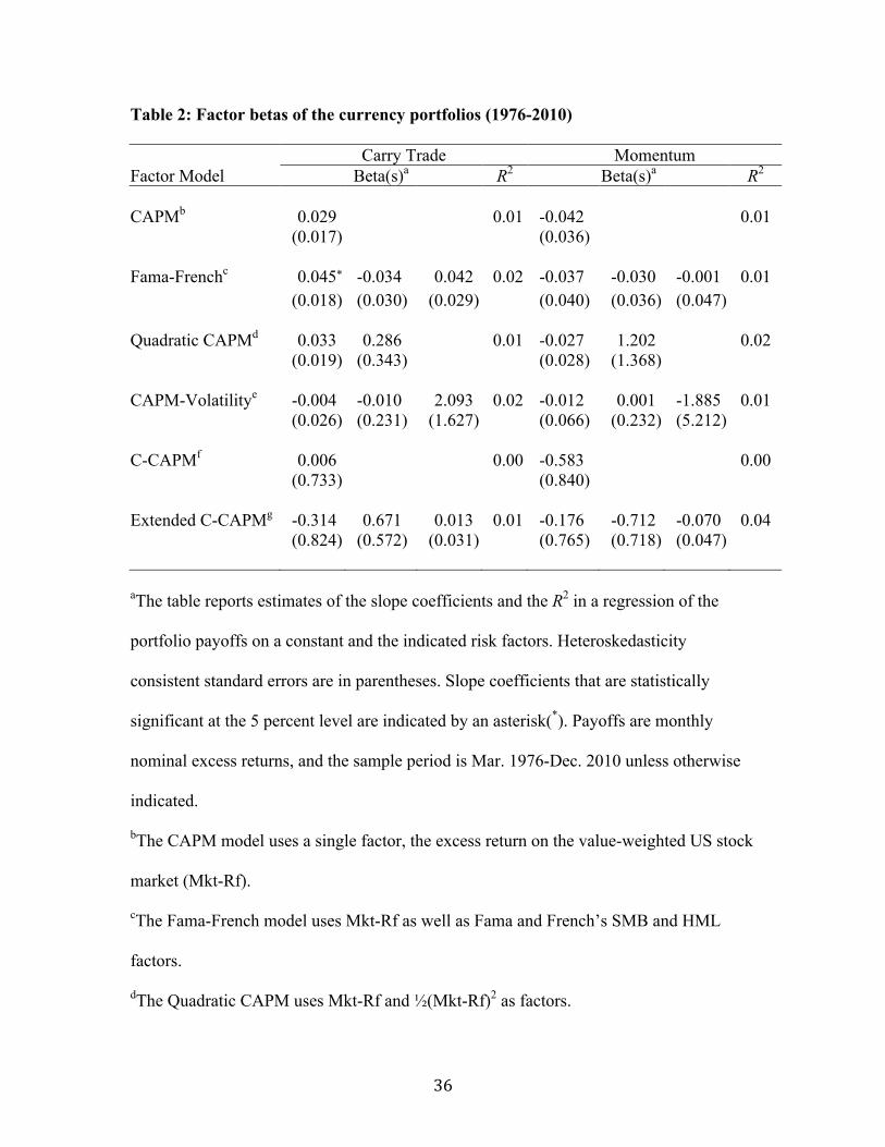
Table 2 summarizes the estimates we obtain by running the time-series regressions de-

scribed by equation (14) for monthly and quarterly models. In every case, but one, we find

that the estimated betas are insignificantly di!erent from zero. The one exception is that

11

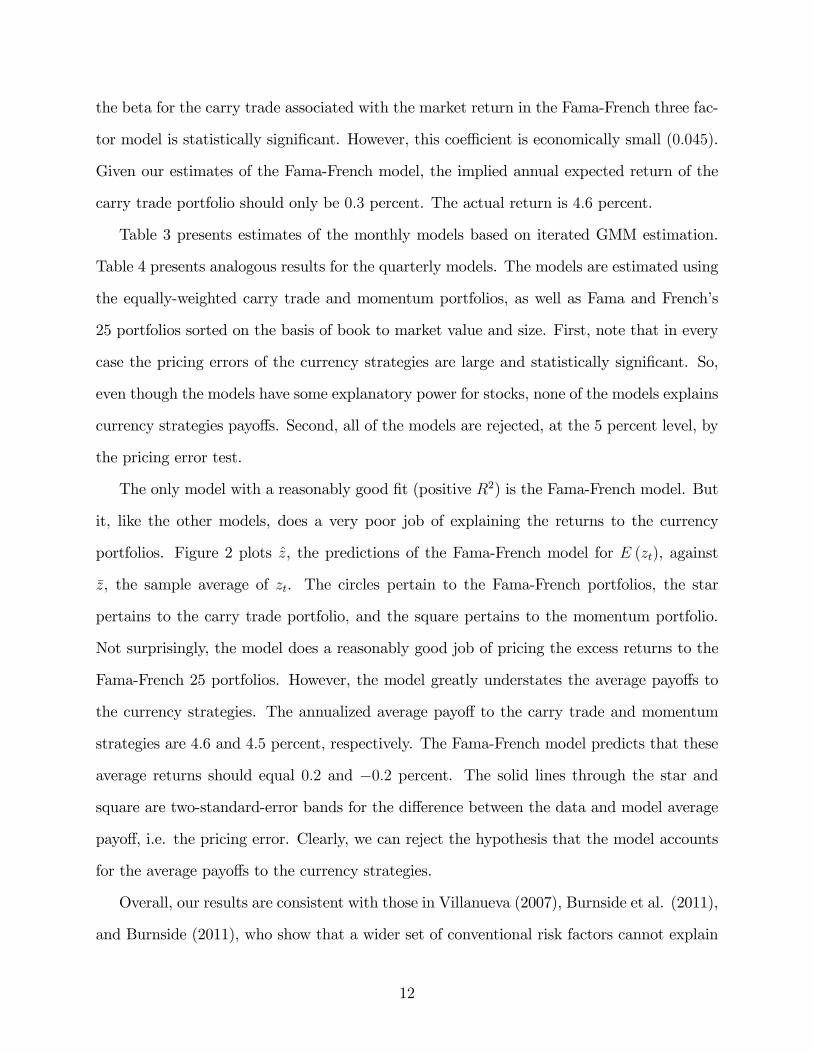
the beta for the carry trade associated with the market return in the Fama-French three fac-

tor model is statistically significant. However, this coe"cient is economically small (0.045).

Given our estimates of the Fama-French model, the implied annual expected return of the

carry trade portfolio should only be 0.3 percent. The actual return is 4.6 percent.

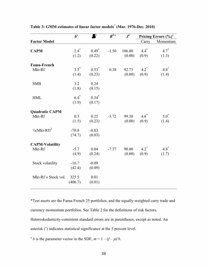
Table 3 presents estimates of the monthly models based on iterated GMM estimation.

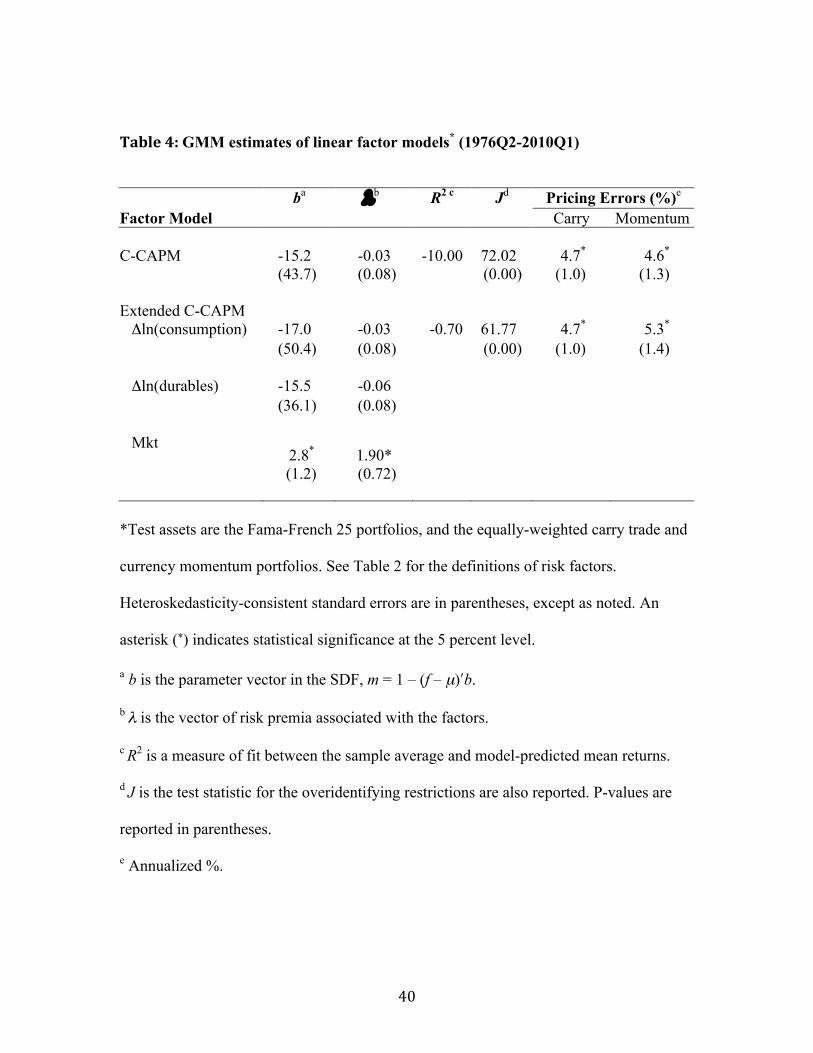
Table 4 presents analogous results for the quarterly models. The models are estimated using

the equally-weighted carry trade and momentum portfolios, as well as Fama and French’s

25 portfolios sorted on the basis of book to market value and size. First, note that in every

case the pricing errors of the currency strategies are large and statistically significant. So,

even though the models have some explanatory power for stocks, none of the models explains

currency strategies payo!s. Second, all of the models are rejected, at the 5 percent level, by

the pricing error test.

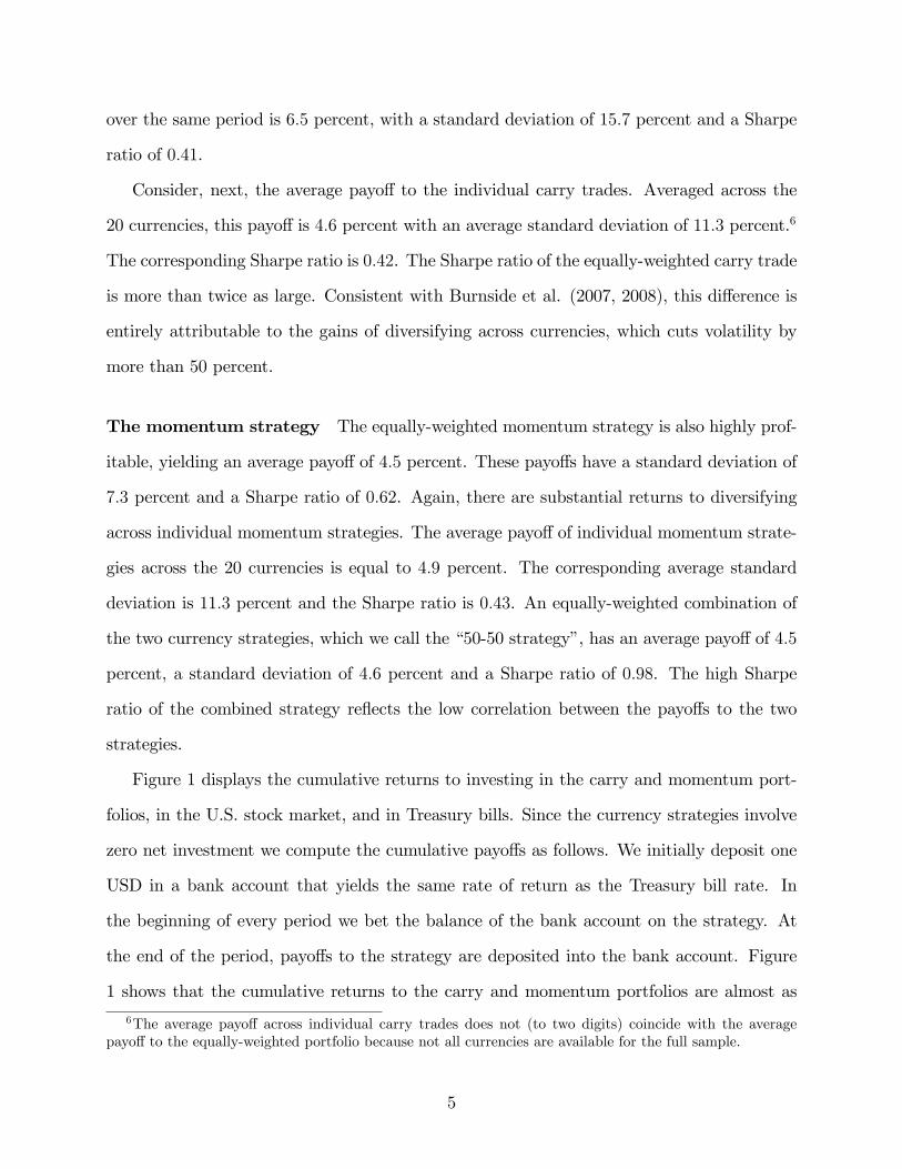
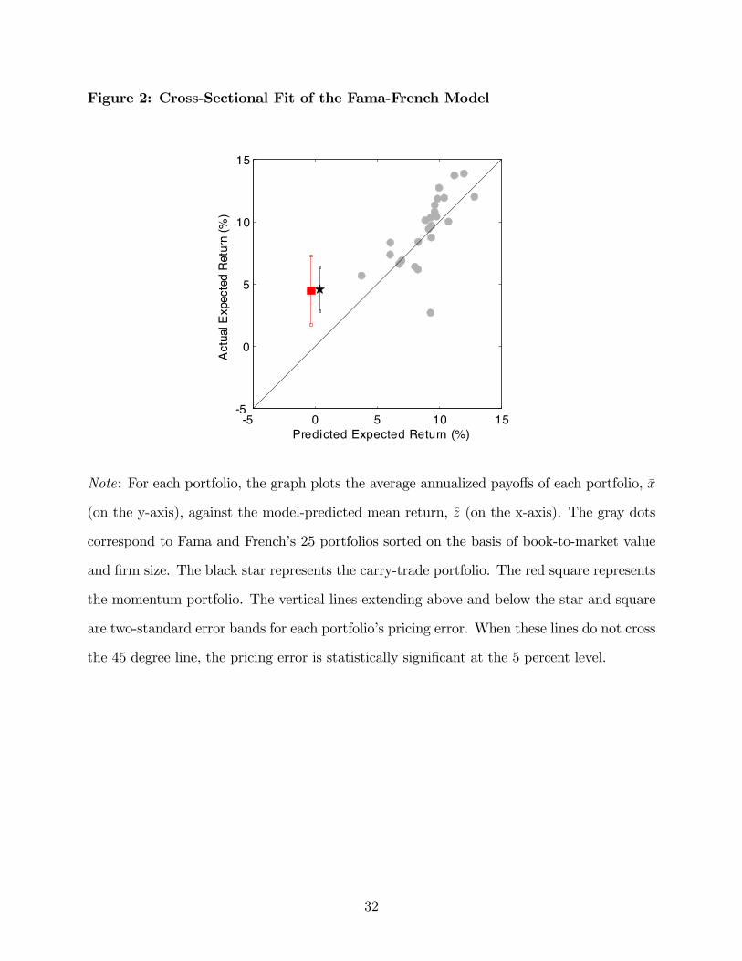
The only model with a reasonably good fit (positive R2) is the Fama-French model. But

it, like the other models, does a very poor job of explaining the returns to the currency

portfolios. Figure 2 plots z, the predictions of the Fama-French model for E (zt), against

z, the sample average of zt. The circles pertain to the Fama-French portfolios, the star

pertains to the carry trade portfolio, and the square pertains to the momentum portfolio.

Not surprisingly, the model does a reasonably good job of pricing the excess returns to the

Fama-French 25 portfolios. However, the model greatly understates the average payo!s to

the currency strategies. The annualized average payo! to the carry trade and momentum

strategies are 4.6 and 4.5 percent, respectively. The Fama-French model predicts that these

average returns should equal 0.2 and !0.2 percent. The solid lines through the star and

square are two-standard-error bands for the di!erence between the data and model average

payo!, i.e. the pricing error. Clearly, we can reject the hypothesis that the model accounts

for the average payo!s to the currency strategies.

Overall, our results are consistent with those in Villanueva (2007), Burnside et al. (2011),

and Burnside (2011), who show that a wider set of conventional risk factors cannot explain

12

the returns to the carry trade. Our results show that conventional risk factors also cannot

explain the returns to the currency momentum portfolio.

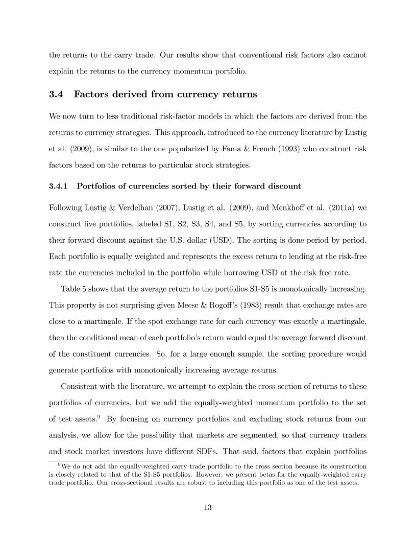
3.4 Factors derived from currency returns

We now turn to less traditional risk-factor models in which the factors are derived from the

returns to currency strategies. This approach, introduced to the currency literature by Lustig

et al. (2009), is similar to the one popularized by Fama & French (1993) who construct risk

factors based on the returns to particular stock strategies.

3.4.1 Portfolios of currencies sorted by their forward discount

Following Lustig & Verdelhan (2007), Lustig et al. (2009), and Menkho! et al. (2011a) we

construct five portfolios, labeled S1, S2, S3, S4, and S5, by sorting currencies according to

their forward discount against the U.S. dollar (USD). The sorting is done period by period.

Each portfolio is equally weighted and represents the excess return to lending at the risk-free

rate the currencies included in the portfolio while borrowing USD at the risk free rate.

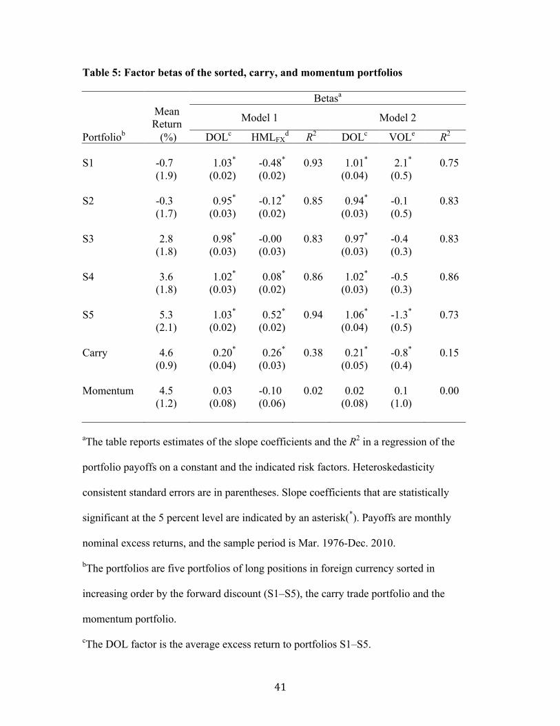
Table 5 shows that the average return to the portfolios S1-S5 is monotonically increasing.

This property is not surprising given Meese & Rogo!’s (1983) result that exchange rates are

close to a martingale. If the spot exchange rate for each currency was exactly a martingale,

then the conditional mean of each portfolio’s return would equal the average forward discount

of the constituent currencies. So, for a large enough sample, the sorting procedure would

generate portfolios with monotonically increasing average returns.

Consistent with the literature, we attempt to explain the cross-section of returns to these

portfolios of currencies, but we add the equally-weighted momentum portfolio to the set

of test assets.9 By focusing on currency portfolios and excluding stock returns from our

analysis, we allow for the possibility that markets are segmented, so that currency traders

and stock market investors have di!erent SDFs. That said, factors that explain portfolios

9We do not add the equally-weighted carry trade portfolio to the cross section because its constructionis closely related to that of the S1-S5 portfolios. However, we present betas for the equally-weighted carrytrade portfolio. Our cross-sectional results are robust to including this portfolio as one of the test assets.

13

S1-S5 should also explain the currency momentum portfolio.

3.4.2 Currency-based risk factors

Like Lustig et al. (2009), we construct two risk factors directly from the sorted portfolios.

The first risk factor, which they call the dollar risk factor and denote by DOL, is simply the

average excess return of the five sorted portfolios. The second risk factor, which they denote

by HMLFX, is the return di!erential between the S5 portfolio (the largest forward discount)

and the S1 portfolio (the smallest forward discount). So, HMLFX is the payo! to a carry

trade strategy in which we go long in the highest forward-discount currencies and go short

in the smallest forward-discount currencies.

Following Menkho! et. al. (2011a), we construct a measure of global currency volatility,

which we denote by VOL. It is measured monthly, and is the average sample standard

deviation of the daily log changes in the values of the currencies in our sample against the

USD.

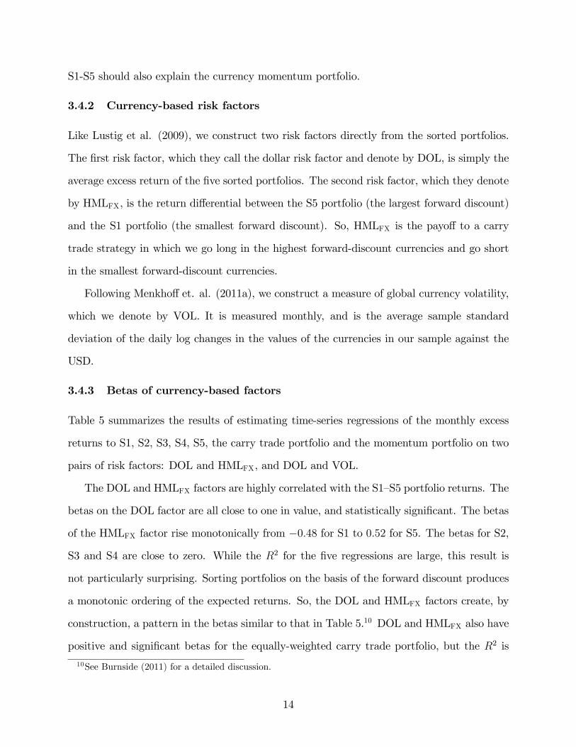
3.4.3 Betas of currency-based factors

Table 5 summarizes the results of estimating time-series regressions of the monthly excess

returns to S1, S2, S3, S4, S5, the carry trade portfolio and the momentum portfolio on two

pairs of risk factors: DOL and HMLFX, and DOL and VOL.

The DOL and HMLFX factors are highly correlated with the S1—S5 portfolio returns. The

betas on the DOL factor are all close to one in value, and statistically significant. The betas

of the HMLFX factor rise monotonically from !0.48 for S1 to 0.52 for S5. The betas for S2,

S3 and S4 are close to zero. While the R2 for the five regressions are large, this result is

not particularly surprising. Sorting portfolios on the basis of the forward discount produces

a monotonic ordering of the expected returns. So, the DOL and HMLFX factors create, by

construction, a pattern in the betas similar to that in Table 5.10 DOL and HMLFX also have

positive and significant betas for the equally-weighted carry trade portfolio, but the R2 is

10See Burnside (2011) for a detailed discussion.

14

much lower in this case. Finally, neither factor has a significant beta for the momentum

portfolio.

Replacing HMLFX with VOL as a factor has very little impact on the betas with respect

to DOL. The betas with respect to VOL decrease monotonically as we go from S1 to S5

and are statistically significant for the extreme portfolios, being positive for S1 and negative

for S5. These findings indicate that when global currency volatility increases, the returns

to holding low-interest rate currencies increase and the returns to holding high-interest rate

currencies decrease. That is, low interest rate currencies provide a hedge against increases

in volatility. The beta with respect to VOL is also negative and statistically significant for

the carry trade portfolio. The beta with respect to VOL is positive but insignificant for the

currency momentum portfolio.

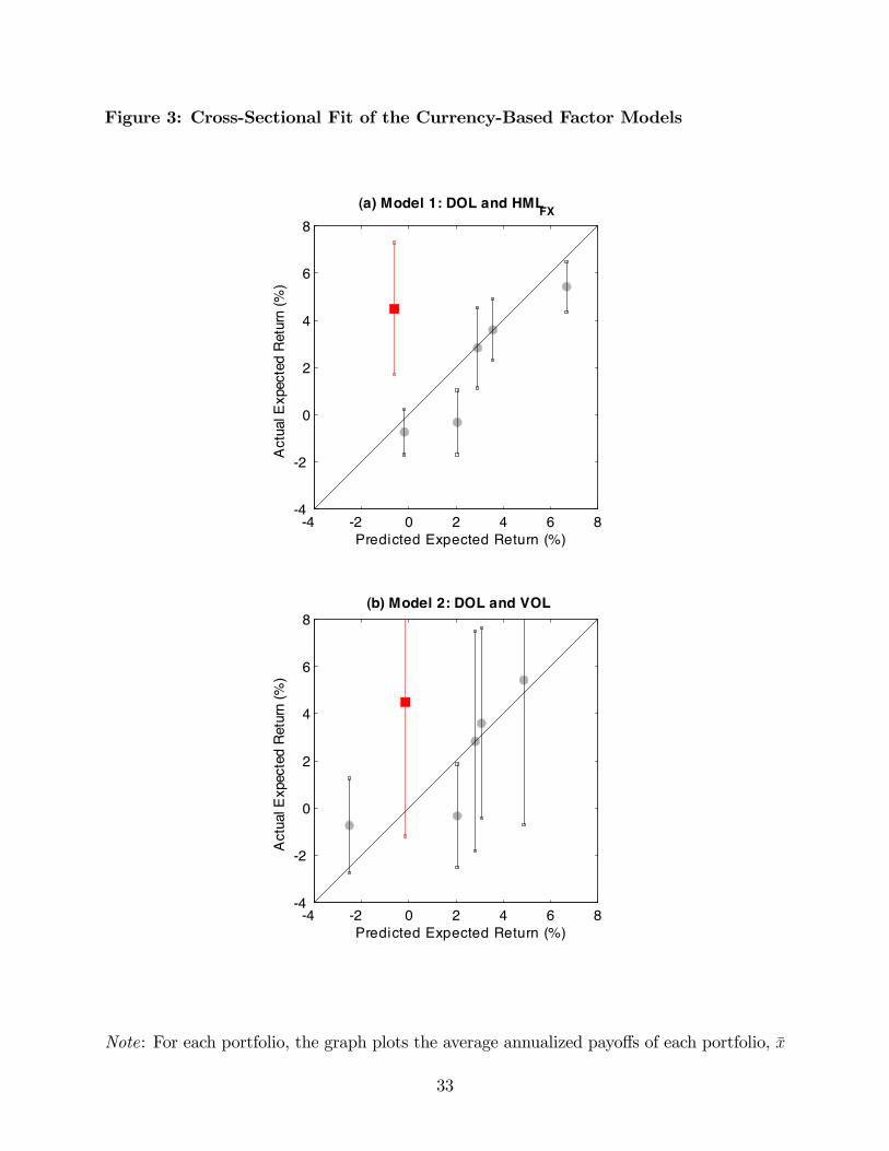
3.4.4 Cross-sectional analysis of currency-based risk factors

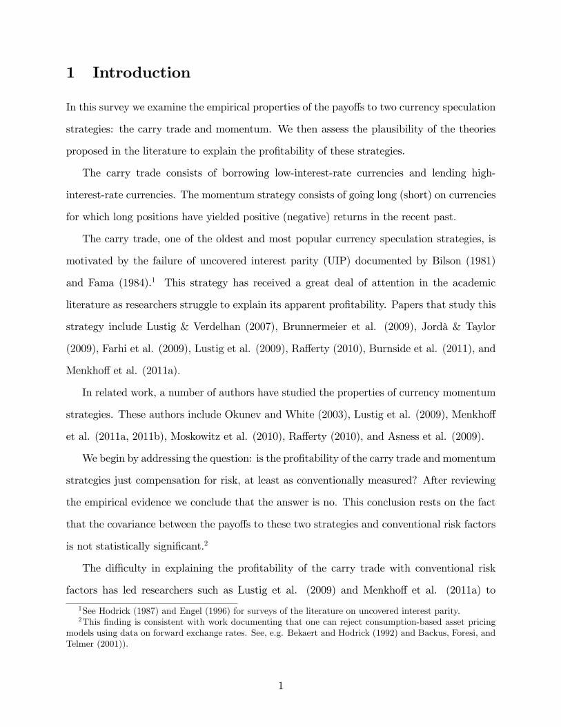
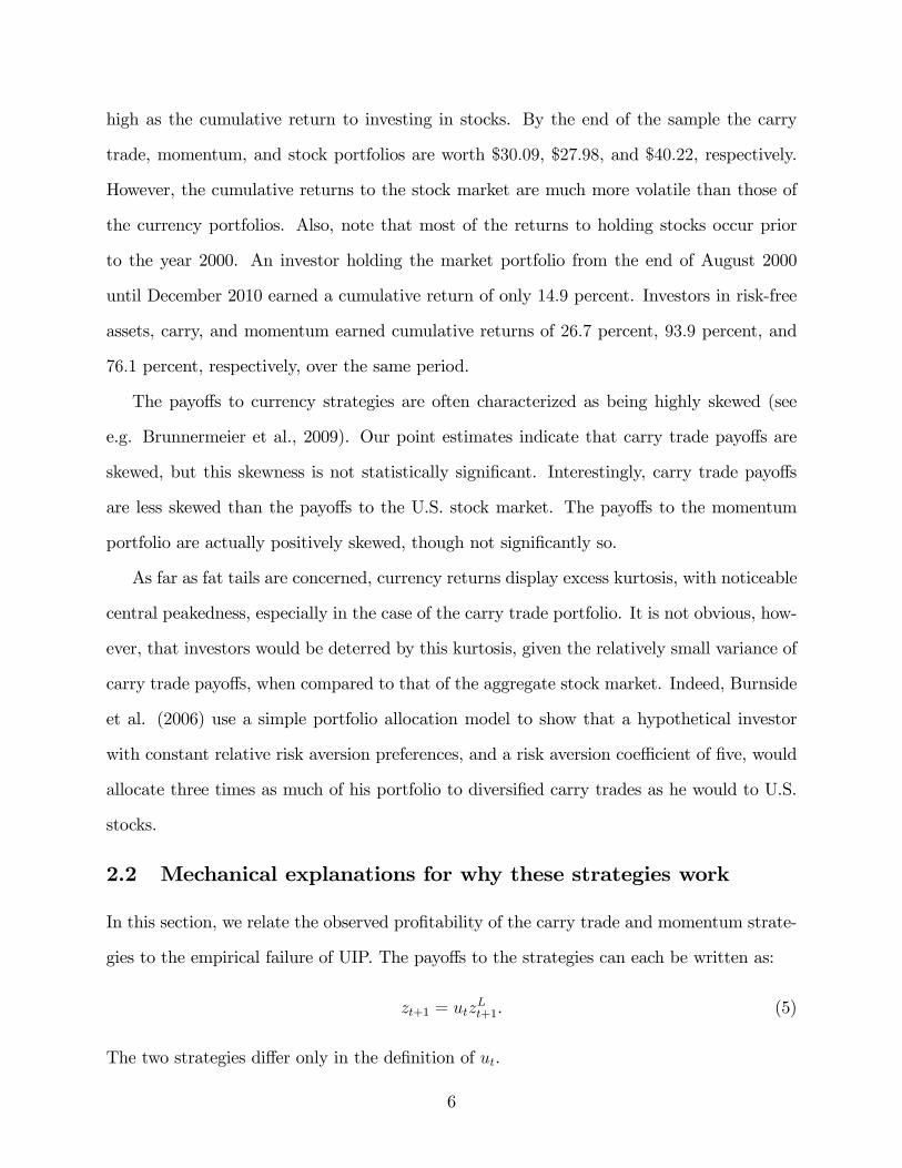
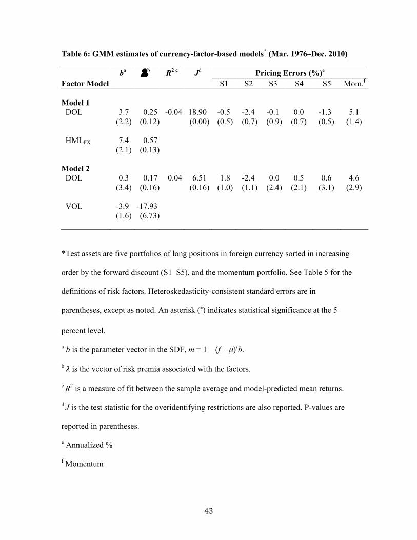
Table 6 presents iterated GMM estimates of the SDF for the two currency-based factor

models, using portfolios S1-S5 and the momentum portfolio as test assets. Figure 3 shows

the mean returns in the sample plotted against the model-predicted expected returns.

In both cases, the b parameter associated with the DOL factor is statistically insignificant.

The risk premium, $DOL, is positive and significant in one case. But in neither case does

exposure to DOL explain much of the variation in expected return across portfolios.

The b and $ parameters associated with the HMLFX factor are positive and statistically

significant at the 5 percent level. The b and $ parameters associated with the VOL factor

are negative and statistically significant at the 5 percent level.

Neither the DOL-HMLFX model nor the DOL-VOL model do a good job of fitting the

overall cross section of average payo!s to the currency strategies. The R2 is lower than 0.04

for both models. The DOL-HMLFX model is rejected on the basis of the pricing-error test.

The DOL-VOL model is not rejected. But this apparent success is mostly due to the model’s

parameters being estimated with less precision than those of the HMLFX-based model.

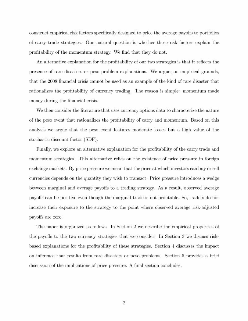
The primary failing of both models is the large pricing error associated with momentum

15

(approximately 5 percent). To understand this failing recall that the average payo! to

the momentum strategy is 4.5 percent. The DOL-HMLFX cannot explain this large payo!

because momentum’s beta is close to zero with respect to DOL and a negative with respect

to HMLFX. The DOL-VOL model does no better because it has a paradoxically positive

(but poorly estimated) beta with respect to VOL, i.e. momentum is a good hedge against

volatility. Menkho! et al. (2011a) find a similar paradox using a set of sorted momentum

portfolios.

3.5 Concluding discussion

The results in this section suggest that observable risk factors explain very little of the average

returns to the carry trade and momentum portfolios, resulting in economically large pricing

errors. In every case the models can also be rejected based on statistical tests of the pricing

errors. Models built from currency specific factors do have some success in explaining the

returns to the carry trade. But, they do not explain the returns to the momentum portfolio.

4 Rare disasters and peso problems

Authors such as Jurek (2008), Farhi & Gabaix (2008), Farhi et al. (2009), and Burnside et

al. (2011) have argued that the payo!s to the carry trade can, at least in part, be explained

by the presence of rare disasters or peso problems.11 By rare disasters we mean very low

probability events that sharply decrease the payo! and/or sharply increase the value of the

SDF. These events may occur in sample. But, due to their low probability, they may be

under-represented relative to their true frequency in population. By a peso problem we mean

an extreme form of this problem, where rare disasters do not occur in sample.

11In this review we focus on recent work that uses options data to study the importance of rare disastersand peso problems. See Evans (2011) for an excellent overview of the earlier literature that uses survey dataand regime-switching models to study how peso problems a!ect conditional inference about the behavior ofexchange rates.

16

Rare disasters We study the e!ects of rare disasters on inference using a simple model.

Let ( % " denote the state of the world, let z(() denote the payo! to a currency strategy

in state (, and M(() denote the value of the SDF in state (. We partition ", the set of

possible states, into two sets. The first set, "N , consists of those values of ( corresponding

to non-rare-disaster (normal) events. The second set, "D, consists of those values of (

corresponding to a rare-disaster event. For simplicity, we assume that "D contains a single

event, (D. We use the notation M " = M((D) and z" = z((D), and assume that z" < 0. To

simplify, we assume that the conditional and unconditional probability of the rare disaster

is p.

Payo!s to a currency strategy must satisfy:

(1! p)EN (Mz) + pM "z" = 0, (18)

whereEN (·) denotes the expectation over normal states. Since the scale ofM is not identified

for zero net investment strategies, we choose the normalization EN(M) = 1.

How can rare disasters explain the profitability of a currency strategy? Assume, for

simplicity, that an econometrician can observe M and z and that the sample average of Mz

across normal events in the sample equals EN(Mz). Suppose that in sample rare disasters

occur with frequency p < p. Since z" < 0, the overall sample average of Mz is positive, even

though the true unconditional value is zero:

(1! p)EN (Mz) + pM "z" = (p! p)%EN (Mz)!M "z"

&> 0.

How likely are we to observe an unusually small number of rare disasters in sample?

Consider the value of p suggested by Nakamura et al. (2010). These authors define a rare

disaster as a large drop in consumption. Using data spanning 24 countries and more than

100 years, they estimate the annual probability of a disaster to be 0.017. The corresponding

monthly value of p is 0.0014.

Since most work on currency strategies focuses on the post Bretton-Woods era, we think

of a typical sample size as roughly (2011 ! 1973) # 12 = 456 months. For p = 0.0014, the

17

expected number of events in a sample of this size is less than one. Indeed, the probability

of observing zero rare disasters in a sample of 456 months is roughly 53 percent.

Can we interpret particular in-sample events as realizations of the rare disaster event

that accounts for the observed profitability of the carry trade and momentum strategies?

For example, was the 2008 financial crisis an example of such a rare disaster? The answer is

no. To see why, note that equation (18) implies that the ratio of risk-adjusted mean payo!s

in the normal states must be equal to the ratio of the payo!s in the disaster state:

EN (Mz1)

EN (Mz2)=z"1z"2. (19)

Here, z"1 and z"2 denote the payo!s to the carry trade and momentum strategy in the disaster

state. We define the disaster period to be August—November 2008 because, during this

period, the carry trade su!ered a cumulative net loss of about 10 percent, its worst loss over

a four month period in our sample. In contrast, the momentum strategy had a cumulative

gain of about 24 percent in this period, its largest over a four month period in our sample. So

the ratio on the right hand side of equation (19) is negative. Since the average risk-adjusted

profits of both strategies are positive outside of the crisis period, the left hand side of equation

(19) is positive. So, the financial crisis is not a plausible example of a rare-disaster event

that accounts for the profitability of the carry trade and momentum strategies. Neither are

other periods in our sample (early 1991, and late 1992) when carry trades took heavy losses.

In these periods the momentum strategy was also highly profitable.

There are two ways to avoid the conclusion that the recent financial crisis is not the

type of rare disaster that accounts for the profitability of the carry trade and momentum

strategies. The first is to assume that, because of market segmentation, M " is di!erent for

the two currency trading strategies. This hypothesis seems very implausible. The second

is to assume that "D contains more than one event, and not all strategies earn negative

returns in all of these events. So the financial crisis could be viewed as a rare disaster in

which the carry trade has a negative payo! but momentum does not. We cannot rule out

this explanation on logical grounds. But it leaves unexplained the in-sample profitability of

18

the momentum strategy.

Peso problems Recall that a peso problem corresponds to the case where there are no rare-

disasters in sample, so p = 0. Absent additional assumptions, the peso-problem explanation

of the profitability of our two strategies has no testable implications, since z" is not observed.

To generate testable implications we assume, as above, that there is a single peso event. We

can then use data on currency options to develop a test of the peso-problem hypothesis.

Investors can use options to construct hedged versions of currency strategies that are

exposed to disaster risk. These hedged strategies put an upper bound on an investor’s

possible losses. Suppose a currency strategy involves going long (short) on foreign currency.

Then this strategy is exposed to large losses if there is a large depreciation (appreciation)

of the foreign currency. By buying a put (call) option on foreign currency the investor can

bound these losses. The payo! to a hedged strategy, zHt+1, is given by

zHt+1 =

*ht+1 if the option is in the money,zt+1 ! ct(1 + it) if the option is out of the money.

The variables ct and it denote the cost of the put or call option and it denotes the nominal

interest rate. The variable ht+1 is the lower bound on the investor’s net payo!.

Since the hedged strategy is also a zero net-investment strategy, its payo!, zH , must

satisfy:

(1! p)EN(MzH) + pM "EN(h) = 0. (20)

Using equation (20) to solve for pM " and replacing this term in equation (18), we obtain:

z" = EN(h)EN (Mz)

EN(MzH). (21)

Motivated by our previous results we assume that covN(M, z) = covN(M, zH) = 0. Then

equation (21) simplifies to:

z" = EN(h)EN (z)

EN(zH). (22)

19

Using equations (18) and (20) we can derive two expressions for ) & pM "/(1 ! p) that are

numerically identical given our method of estimating z":

) = !EN (z)

z"= !

EN(zH)

EN(h). (23)

Here, we estimate ) because the parameters p and M " are not separately identified by the

pricing equations.

We estimate z" and ) for the carry trade using currency option data from J.P. Morgan for

ten major currencies over the period 1995—2009. As in Burnside et al. (2011), we assume that

in the disaster state all of the individual currency carry trades lose money. Consequently,

we assume that the investor hedges the equally-weighted carry trade strategy by buying

at-the-money options. This assumption means that the payo! of the carry trade portfolio in

the peso state is the average of the minimum payo!s of the individual carry trades in that

state.

The momentum strategy for an individual currency sometimes takes the opposite position

of the carry trade strategy. In these instances, if we assume carry is exposed to disaster

risk, momentum is naturally hedged against it. This property presents a di"culty for our

empirical strategy because it means that the unhedged momentum payo! for an individual

currency in the disaster state is occasionally !z", rather than z".

To bring momentum into our analysis, we consider a 50-50 portfolio that equally combines

the carry trade and momentum portfolios. Suppose each of these portfolios is formed with n

currencies. When the two underlying strategies agree on the sign of an individual currency

trade, the net position in the portfolio for that currency is ±1/n. In this case, the position is

naturally exposed to disaster risk, and this risk can be hedged using options. When the two

underlying strategies disagree on the sign of an individual currency trade, the net position

for that currency is zero.

Using data on the payo!s to the hedged and unhedged carry trade and 50-50 carry-

momentum strategies, and data on the minimum payo!s to the hedged strategies, we estimate

the moments that appear on the right hand sides of equations (22) and (23). Doing so

20

provides us with estimates of z"1 (the payo! to the equally-weighted carry trade in the disaster

state) and z"2 (the payo! to the 50-50 strategy in the disaster state), and two estimates of ).

Using a Wald test, we can test whether the two estimates of ) are equal, which they should

be, in absence of market segmentation.12 Alternatively, we can use the pricing equations of

the hedged and unhedged versions of the two strategies to estimate the three parameters, z"1

and z"2 and ) using GMM. This system is overidentified, and, therefore, provides us with a

simple test of the peso problem hypothesis.

When we use the first procedure, our estimates are z"1 = !0.037 (0.014), z"2 = !0.019

(0.006). Standard errors are reported in parenthesis. Our two estimates of ) are 0.095

(0.059) and 0.159 (0.091). The two estimates of ) are insignificantly di!erent from each other

according to the Wald test (p-value = 0.23). Given the small standard errors associated with

z"1 and z"2, we can be quite confident that the disaster event is not characterized by large

losses to either the carry trade or the 50-50 carry-momentum portfolio.

When we use the second procedure, our estimates of z"1 and z"2 are !0.040 (0.020) and

!0.027 (0.015), and our estimate of ) is 0.089 (0.064). The test of the overidentifying

restrictions does not reject the model (p-value = 0.27). A value of ) of 0.089 means that if

we assume that the true probability of a rare event is p = 0.0014, then M " "= 63.

Our analysis assumes that the SDF takes on a single value in the rare disaster or peso

state. Under alternative assumptions, we can still generate testable implications of the peso

problem hypothesis. For example, Burnside et al. (2011) show how to estimate a lower

bound for ED(z1) allowing for negative covariance between payo!s to the carry trade and

the SDF in the peso state.

Overall, we find little evidence against the peso event hypothesis. According to our point

estimates, the peso event is not characterized by large losses to the currency strategies.

Instead, it is characterized by moderate losses and large values of the SDF.

12Burnside et al. (2011) discuss a related comparison of the values of M ! implied by the carry trade anda hedged stock market strategy.

21

5 Price pressure

In this section we discuss an alternative explanation for the profitability of our currency

strategies raised in Burnside et al. (2006). This explanation relies on the existence of price

pressure in the foreign exchange market. By price pressure we mean that the price at which

investors can buy or sell an asset depends on the quantity they wish to transact. There is

a strand of research in finance that stresses the possibility that demand curves for assets

are downward sloping. Shleifer (1986) and Mitchell & Pulvino (2004) present evidence in

support of this view for stocks.

Anecdotal evidence gathered from currency traders suggests that a similar phenomenon

occurs in foreign exchange markets: prices move against individual traders when they place

large orders. Here we present a simple model that illustrates the implications of price pressure

for the profitability of currency-trading strategies.

The case of a single trader Consider an asset that has a value v+*, where * is a random

variable with mean zero. Suppose that there is a single risk-neutral trader who decides to

buy x units of the asset. To capture the basic e!ects of price pressure we suppose that the

price of the asset that the trader purchases depends on order size in the following way. The

price in the beginning of the day is:

p0 = a. (24)

As long as a < v, it is optimal for the trader to buy a positive quantity of the asset. Trading

takes place during the course of a day. At instant t during the day the change in the price

depends on the quantity of orders, mt, submitted at that point in time:

pt = bmt. (25)

We assume that b is positive, so that the price is an increasing function of the quantity

purchased, i.e., there is price pressure.

Suppose the trader wants to buy x units of currency during the day. Consider the

22

following two strategies. Strategy A is to submit an order for x, say, at the end of the day.

The price associated with the order is a+bx, so that the total cost of the order is: x (a+ bx).

Strategy B is to break up the order and submit orders of size m = x/T throughout the

day. Here, T is the number of trading minutes in the day. The price of the asset at time t

is given by:

pt = a+ b

+ t

0

msds = a+ bx

Tt.

The total cost of the order is:+ T

0

ptx

Tdt = ax+ b

1

2x2.

It is clear that, from the perspective of the trader, strategy B dominates strategy A. So, we

assume that the trader uses strategy B and breaks up the orders. It is useful to re-write the

total cost of the order as:, x0(a+ bz)dz.

The trader’s profit, +, is given by:

+ = (v + *)x!+ x

0

(a+ bz)dz.

The trader chooses x to maximize the expected value of +:

E (+) = vx!+ x

0

(a+ bz)dz.

The first-order condition for this problem implies that the optimal value of x, x!, is given

by:

x! =v ! ab.

The price paid for the last unit of the asset purchased is:

p! = v.

We wish to stress two key features of this example. First, the expected profit from the last

unit of the asset purchased by the trader is equal to zero. Second, the total expected profits

earned by the trader are positive:

E(+) =1

2

(v ! a)2

b.

23

Consider an econometrician who observes the average trade during the day. He would cor-

rectly infer that the strategy is profitable. Suppose that he ignores the existence of price

pressure and assumes that marginal and average profits coincide. Then he would incorrectly

conclude that the trader is leaving money on the table by not expanding the size of the

trade.

The case of n traders Suppose that there is a fixed number, n, of traders. Within the

day price pressure is governed by equations (24) and (25) where mt denotes total orders

arriving at time t. Consider a Nash equilibrium in which each trader chooses to buy x units

of the asset taking as given that the remaining n ! 1 traders buy x units each. The order

in which trades occur is randomly determined after traders choose x. Trader j trades from

time T (j ! 1)/n to time Tj/n, where the index j takes values from one to n. Each trader

breaks up his orders uniformly within his trading period. Since a representative trader has

a probability 1/n of being the jth trader, his expected profit is:

E (+) = vx!n#1-

j=0

1

n

+ jx+x

jx

(a+ bz)dz.

The optimal value of x satisfies the first-order condition:

v = a+ bx+1

2bx (n! 1)

In a symmetric equilibrium x = x, so:

x =2 (v ! a)b(1 + n)

. (26)

The average expected profit across traders is positive and equal to:

E (+) =2 (v ! a)2

b(1 + n)2> 0.

The expected profit of a trader who has a position j in the trading queue is:

E (+j) =2

b

(v ! a)2

(1 + n)2[n+ 2(1! j)] .

24

So, when n is large, roughly half of the traders make profits and the other half make losses.

The profits of the winners are larger than the losses of the losers, which is why average profits

across traders are positive.

As in the single trader case, an econometrician who observes the average trade during

the day would conclude that the strategy is profitable. He might wonder why traders don’t

increase their positions until this profitability vanishes. But, while the average trade gener-

ates profits, the marginal trade makes losses. So, there is no reason for traders to expand

their positions. No money is being left on the table.

6 Conclusion

We discuss two conventional explanations for the apparent profitability of the carry trade

and momentum strategies. The first is that investors are compensated for the risk they bear.

While this hypothesis is very appealing, we find little evidence to support it. The second

conventional explanation is that the profitability of the two currency strategies results from

a rare disaster or peso problem. We argue that the recent financial crisis is not a rare disaster

from the standpoint of a currency speculator who uses both the carry trade and momentum

strategies. We also argue that the peso event is not characterized by large losses to currency

speculators. Instead, it features moderate losses and high values of the stochastic discount

factor.

Finally, we discuss the potential role of price pressure in explaining the profitability

of the two currency strategies. While this approach shows some promise, two important

questions remain to be answered. First, is the form of price pressure postulated in our

example empirically plausible for currency markets? Second, what is the source of this price

pressure?

25

Literature Cited

Asness CS, Moskowitz TJ, Pedersen LH. 2009. Value and momentum everywhere. Mimeo,

University of Chicago.

Backus DK, Foresi S, Telmer CI. 2001. A"ne term structure models and the forward

premium anomaly. J. Financ. 56(1):279—304.

Bekaert G, Hodrick RJ. 1992. Characterizing predictable components in excess returns on

equity and foreign exchange markets. J. Financ. 47(2):467—509.

Bilson JFO. 1981. The ‘Speculative E"ciency’ hypothesis. J. Bus. 54(3):435—51.

Brunnermeier MK, Nagel S, Pedersen LH. 2009. Carry trades and currency crashes. NBER

Macroecon. Ann. 23:313—47.

Burnside C. 2007. The cross-section of foreign currency risk premia and consumption

growth risk: A comment. NBER Working Paper 13129.

Burnside C. 2011. Carry trades and risk. Forthcoming in The Handbook of Exchange Rates,

James J, Marsh IW, Sarno L, eds. Hoboken, NJ: Wiley

Burnside C, Eichenbaum M, Kleshchelski I, Rebelo S. 2006. The returns to currency spec-

ulation. NBER Working Paper 12489.

Burnside C, Eichenbaum M, Kleshchelski I, Rebelo S. 2011. Do peso problems explain the

returns to the carry trade? Rev. Financ. Stud. 24(3):853—91.

Burnside C, Eichenbaum M, Rebelo S. 2007. The returns to currency speculation in emerg-

ing markets. Am. Econ. Assoc. 97(2):333-8.

Burnside C, Eichenbaum M, Rebelo S. 2008, Carry trade: The gains of diversification. J.

Eur. Econ. Assoc. 6(2-3):581—8.

26

Carhart M. 1997. On persistence in mutual fund performance. J. Financ. 52(1):57—82.

Clinton K. 1988. Transactions costs and covered interest arbitrage: Theory and evidence.

J. Polit. Econ. 96(2):358—70.

Engel C. 1996. The forward discount anomaly and the risk premium: A survey of recent

evidence. J. Empir. Financ. 3(2):123—92.

Evans, M. 2011. Exchange rate dynamics. Princeton University Press.

Fama EF. 1984. Forward and spot exchange rates. J. Monetary Econ. 14(3):319—38.

Fama EF, French KR. 1993. Common risk factors in the returns on stocks and bonds. J.

Financ. Econ. 33(1):3—56.

Farhi E, Fraiberger SP, Gabaix X, Ranciere R, Verdelhan A. 2009. Crash risk in currency

markets. NBER Working Paper 15062.

Farhi E, Gabaix X. 2008. Rare disasters and exchange rates. NBER Working Paper 13805.

Hansen LP. 1982. Large sample properties of generalized method of moments estimators.

Econometrica 50(4):1029—54.

Harvey CR, Siddique A. 2000. Conditional skewness in asset pricing tests. J. Financ.

55(3):1263—95.

Hodrick RJ. 1987. The Empirical Evidence on the E!ciency of Forward and Futures Foreign

Exchange Markets. Chur, Switzerland: Harwood Academic Publishers

Jegadeesh N, Titman S. 1993. Returns to buying winners and selling losers: Implications

for stock market e"ciency. J. Financ. 48(1):65—91.

Jordà Ò, Taylor AM. 2009. The carry trade and fundamentals: Nothing to fear but FEER

itself. NBER Working Paper 15518.

27

Jurek JW. 2008. Crash-neutral currency carry trades. Mimeo, Princeton University. SSRN

Paper 1262934.

Lintner J. 1965. The valuation of risk assets and the selection of risky investments in stock

portfolios and capital budgets. Rev. Econ. Stat. 47(1):13—37.

Lustig H, Roussanov N, Verdelhan A. 2009. Common risk factors in currency markets.

SSRN Paper 1139447.

Lustig H, Verdelhan A. 2007. The cross-section of foreign currency risk premia and con-

sumption growth risk. Am. Econ. Rev. 97(1):89—117.

Mancini-Gri!oli T, Ranaldo A. 2011. Limits to arbitrage during the crisis: funding liquidity

constraints and covered interest parity. SSRN Paper 1549668.

Meese RA, Rogo! K. 1983. Empirical exchange rate models of the seventies: Do they fit

out of sample? J. Int. Econ. 14(1-2):3—24.

Menkho! L, Sarno L, Schmeling M, Schrimpf A. 2011a. Carry trades and global foreign

exchange volatility. Forthcoming, J. Financ.

Menkho! L, Sarno L, Schmeling M, Schrimpf A. 2011b. Currency momentum strategies.

Mimeo. Cass Business School, City University, London.

Mitchell M, Pulvino T. 2004. Price pressure around mergers. J. Financ. 59(1):31—63.

Moskowitz T, Ooi YH, Pedersen LH. 2010. Time series momentum. Mimeo, New York

University.

Nakamura E, Steinsson J, Barro RJ, Ursúa JF. 2010. Crises and recoveries in an empirical

model of consumption disasters. NBER Working Paper 15920.

Okunev J, White D. 2003. Do momentum-based strategies still work in foreign currency

markets? J. Financ. Quant. Anal. 38(2):425—47.

28

Ra!erty B. 2010. The returns to currency speculation and global currency realignment risk.

Mimeo, Duke University.

Rouwenhorst KG. 1998. International momentum strategies. J. Financ. 53(1):267—84.

Sharpe WF. 1964. Capital asset prices: a theory of market equilibrium under conditions of

risk. J. Financ. 19(3):425—42.

Shleifer A. 1986. Do demand curves for stocks slope down? J. Financ. 41(3):579—90.

Taylor, MP. 1987. Covered interest parity: A high-frequency, high-quality data study.

Economica 54 (216):429—38.

Taylor, MP. 1989. Covered interest arbitrage and market turbulence. Econ. J. 99(396):376—

91.

Villanueva OM. 2007. Forecasting currency excess returns: Can the forward bias be ex-

ploited? J. Financ. Quant. Anal. 42(4):963—90.

Yogo M. 2006. A consumption-based explanation of expected stock returns. J. Financ.

61(2):539—80.

29

!"#$%& '( )$*$+,-".& /&-$%01 23 40.&1-*&0- 5-%,-&#"&1! !&67 '89:;<&=7 >?'?

76 78 80 82 84 86 88 90 92 94 96 98 00 02 04 06 08 10

1

2

4

8

16

32

64$

on a

log

scal

e (J

an-1

976=

1)US StocksCarryMomentumT-Bi l ls

!"#$" #$% &'()% *+,-. -$% /(0(+1-23% )%-()4. ,5 1 -)16%) 7$, 8%'24. 72-$ 9 6,++1) 24 :14(1);

9<=> 146 243%.-. $2. 1//(0(+1-%6 %1)424'. %?/+(.23%+; 24 ,4% ,5 5,() .-)1-%'2%.@ A,) #B82++.

146 CD .-,/E. 7% (.% -$% )2.E 5)%% )1-% 146 31+(%B7%2'$-%6 01)E%- )%-()4 )%*,)-%6 24 F%44%-$

A)%4/$G. 61-181.%@ H%-12+. 5,) -$% /1)); -)16% 146 0,0%4-(0 .-)1'%-2%. 1)% *),326%6 24 -$%

-%?-@

I9

!"#$%& '( )%*++,-&./"*012 !"/ *3 /4& !151,!%&0.4 6*7&2

-5 0 5 10 15-5

0

5

10

15

Predicted Expected Return (%)

Act

ual E

xpec

ted

Retu

rn (%

)

!"#$! "#$ %&'( )#$*+#,-#. *(% /$&)( ),#*0 *(% &1%$&/% &223&,-4%5 )&6#70 #+ %&'( )#$*+#,-#. !!

8#2 *(% 69&:-0;. &/&-20* *(% <#5%,9)$%5-'*%5 <%&2 $%*3$2. "" 8#2 *(% :9&:-0;= >(% /$&6 5#*0

'#$$%0)#25 *# "&<& &25 "$%2'(?0 @A )#$*+#,-#0 0#$*%5 #2 *(% B&0-0 #+ B##C9*#9<&$C%* 1&,3%

&25 D$< 0-4%= >(% B,&'C 0*&$ $%)$%0%2*0 *(% '&$$69*$&5% )#$*+#,-#= >(% $%5 0E3&$% $%)$%0%2*0

*(% <#<%2*3< )#$*+#,-#= >(% 1%$*-'&, ,-2%0 %:*%25-2/ &B#1% &25 B%,#F *(% 0*&$ &25 0E3&$%

&$% *F#90*&25&$5 %$$#$ B&250 +#$ %&'( )#$*+#,-#?0 )$-'-2/ %$$#$= G(%2 *(%0% ,-2%0 5# 2#* '$#00

*(% HA 5%/$%% ,-2%. *(% )$-'-2/ %$$#$ -0 0*&*-0*-'&,,6 0-/2-D'&2* &* *(% A )%$'%2* ,%1%,=

I@

!"#$%& '( )%*++,-&./"*012 !"/ *3 /4& )$%%&0.5,61+&7 !1./*% 8*7&2+

-4 -2 0 2 4 6 8-4

-2

0

2

4

6

8

Predicted Expected Return (%)

Act

ual E

xpec

ted

Retu

rn (%

)

(a) Model 1: DOL and HMLFX

-4 -2 0 2 4 6 8-4

-2

0

2

4

6

8

Predicted Expected Return (%)

Act

ual E

xpec

ted

Retu

rn (%

)

(b) Model 2: DOL and VOL

!"#$! "#$ %&'( )#$*+#,-#. *(% /$&)( ),#*0 *(% &1%$&/% &223&,-4%5 )&6#70 #+ %&'( )#$*+#,-#. !!

88

!"# $%& '()*+,-. )/)+#,$ $%& 0"1&2(34&1+5$&1 0&)# 4&$64#. !! !"# $%& *()*+,-7 8%& /4)' 1"$,

5"44&,3"#1 $" $%& 9:;9< 5644&#5' 3"4$="2+", ,"4$&1 "# $%& >),+, "= $%& ="4?)41 1+,5"6#$7 8%&

4&1 ,@6)4& 4&34&,&#$, $%& 0"0&#$60 3"4$="2+"7 8%& A&4$+5)2 2+#&, &*$&#1+#/ )>"A& )#1 >&2"?

&)5% 3"+#$ )4& $?"(,$)#1)41 &44"4 >)#1, ="4 &)5% 3"4$="2+"B, 34+5+#/ &44"47 C%&# $%&,& 2+#&,

1" #"$ 54",, $%& D< 1&/4&& 2+#&. $%& 34+5+#/ &44"4 +, ,$)$+,$+5)22' ,+/#+E5)#$ )$ $%& < 3&45&#$

2&A&27

FD

! "#!

Table 1: Annualized excess returns of investment strategies (Feb. 1976-Dec. 2010) Mean SD Sharpe Skewness Excess Correlation with (%) (%) Ratio Kurtosis Carry Momentum Individual currency strategies (average)a Carry trade 4.6 11.3 0.42 -0.23 1.6 Momentum trade 4.9 11.3 0.43 -0.02 1.5 Portfolio strategiesb Carry tradec 4.6 5.1 0.89 -0.53 4.1 1.00 0.10 (0.9) (0.4) (0.21) (0.40) (1.5) Momentumc 4.5 7.3 0.62 0.08 2.9 0.10 1.00 (1.2) (0.5) (0.16) (0.32) (0.9) 50-50 strategyd 4.5 4.6 0.98 0.36 2.5 0.63 0.84 (0.8) (0.3) (0.16) (0.22) (0.5) U.S. stockse 6.5 15.7 0.41 -0.78 2.3 0.09 -0.09 (2.8) (1.0) (0.19) (0.28) (1.1)

aThe mean excess returns of the currency portfolios are not equal to the average mean

excess returns of the respective individual-currency trades because the sample period

varies by currency.

bHeteroskedasticity-consistent GMM standard errors are in parentheses.

cThe carry trade (momentum) portfolio is formed as the average of up to 20 individual

currency carry (momentum) trades against the USD.

dThe 50-50 strategy is an equally-weighted average of the carry and momentum

portfolios.

eThe U.S. stock market return is the value-weighted excess return on all U.S. stocks.

! "#!

Table 2: Factor betas of the currency portfolios (1976-2010)

Carry Trade Momentum Factor Model Beta(s)a R2 Beta(s)a R2 CAPMb 0.029 0.01 -0.042 0.01 (0.017) (0.036) Fama-Frenchc 0.045* -0.034 0.042 0.02 -0.037 -0.030 -0.001 0.01 (0.018) (0.030) (0.029) (0.040) (0.036) (0.047) Quadratic CAPMd 0.033 0.286 0.01 -0.027 1.202 0.02 (0.019) (0.343) (0.028) (1.368) CAPM-Volatilitye -0.004 -0.010 2.093 0.02 -0.012 0.001 -1.885 0.01 (0.026) (0.231) (1.627) (0.066) (0.232) (5.212) C-CAPMf 0.006 0.00 -0.583 0.00 (0.733) (0.840) Extended C-CAPMg -0.314 0.671 0.013 0.01 -0.176 -0.712 -0.070 0.04 (0.824) (0.572) (0.031) (0.765) (0.718) (0.047) aThe table reports estimates of the slope coefficients and the R2 in a regression of the

portfolio payoffs on a constant and the indicated risk factors. Heteroskedasticity

consistent standard errors are in parentheses. Slope coefficients that are statistically

significant at the 5 percent level are indicated by an asterisk(*). Payoffs are monthly

nominal excess returns, and the sample period is Mar. 1976-Dec. 2010 unless otherwise

indicated.

bThe CAPM model uses a single factor, the excess return on the value-weighted US stock

market (Mkt-Rf).

cThe Fama-French model uses Mkt-Rf as well as Fama and French’s SMB and HML

factors.

dThe Quadratic CAPM uses Mkt-Rf and !(Mkt-Rf)2 as factors.

! "#!

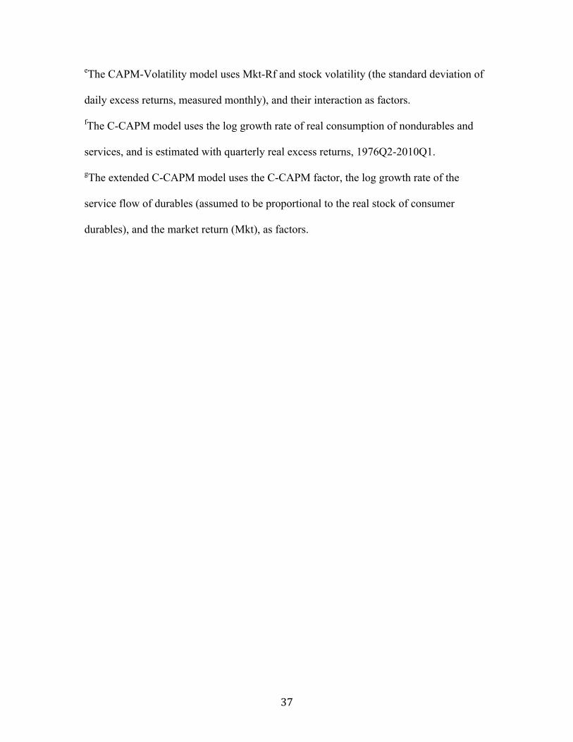
eThe CAPM-Volatility model uses Mkt-Rf and stock volatility (the standard deviation of

daily excess returns, measured monthly), and their interaction as factors.

fThe C-CAPM model uses the log growth rate of real consumption of nondurables and

services, and is estimated with quarterly real excess returns, 1976Q2-2010Q1.

gThe extended C-CAPM model uses the C-CAPM factor, the log growth rate of the

service flow of durables (assumed to be proportional to the real stock of consumer

durables), and the market return (Mkt), as factors.

! "#!

Table 3: GMM estimates of linear factor models* (Mar. 1976-Dec. 2010) ba !b R2 c Jd Pricing Errors (%)e Factor Model Carry Momentum CAPM 2.4* 0.49* -1.50 106.00 4.4* 4.7* (1.2) (0.22) (0.00) (0.9) (1.3) Fama-French Mkt-Rf 3.5* 0.53* 0.38 92.73 4.2* 4.8* (1.4) (0.23) (0.00) (0.9) (1.4) SMB 3.2 0.24 (1.8) (0.15) HML 6.4* 0.34* (1.9) (0.17) Quadratic CAPM Mkt-Rf 0.3 0.25 -3.72 99.38 4.6* 5.0* (1.5) (0.23) (0.00) (0.9) (1.4) !(Mkt-Rf)2 -70.8 -0.03 (74.7) (0.03) CAPM-Volatility Mkt-Rf -5.7 0.04 -7.37 90.80 4.2* 4.8* (4.9) (0.24) (0.00) (0.9) (1.7) Stock volatility -16.7 -0.09 (42.4) (0.09) Mkt-Rf ! Stock vol. 325.5 0.01 (406.7) (0.01)

*Test assets are the Fama-French 25 portfolios, and the equally-weighted carry trade and

currency momentum portfolios. See Table 2 for the definitions of risk factors.

Heteroskedasticity-consistent standard errors are in parentheses, except as noted. An

asterisk (*) indicates statistical significance at the 5 percent level.

a b is the parameter vector in the SDF, m = 1 – (f – µ)"b.

! "#!

b ! is the vector of risk premia associated with the factors.

c R2 is a measure of fit between the sample average and model-predicted mean returns.

d J is the test statistic for the overidentifying restrictions are also reported. P-values are

reported in parentheses.

e Annualized %.

! "#!

!"#$%&'(&GMM estimates of linear factor models* (1976Q2-2010Q1) ba !b R2 c Jd Pricing Errors (%)e Factor Model Carry Momentum C-CAPM -15.2 -0.03 -10.00 72.02 4.7* 4.6* (43.7) (0.08) (0.00) (1.0) (1.3) Extended C-CAPM !ln(consumption) -17.0 -0.03 -0.70 61.77 4.7* 5.3* (50.4) (0.08) (0.00) (1.0) (1.4) ! !ln(durables) -15.5 -0.06 (36.1) (0.08) ! Mkt

2.8* 1.90*

(1.2) (0.72) *Test assets are the Fama-French 25 portfolios, and the equally-weighted carry trade and

currency momentum portfolios. See Table 2 for the definitions of risk factors.

Heteroskedasticity-consistent standard errors are in parentheses, except as noted. An

asterisk (*) indicates statistical significance at the 5 percent level.

a b is the parameter vector in the SDF, m = 1 – (f – µ)"b.

b ! is the vector of risk premia associated with the factors.

c R2 is a measure of fit between the sample average and model-predicted mean returns.

d J is the test statistic for the overidentifying restrictions are also reported. P-values are

reported in parentheses.

e Annualized %.

! "#!

Table 5: Factor betas of the sorted, carry, and momentum portfolios Betasa

Mean Return Model 1 Model 2

Portfoliob (%) DOLc HMLFXd R2 DOLc VOLe R2

S1 -0.7 1.03* -0.48* 0.93 1.01* 2.1* 0.75 (1.9) (0.02) (0.02) (0.04) (0.5) S2 -0.3 0.95* -0.12* 0.85 0.94* -0.1 0.83 (1.7) (0.03) (0.02) (0.03) (0.5) S3 2.8 0.98* -0.00 0.83 0.97* -0.4 0.83 (1.8) (0.03) (0.03) (0.03) (0.3) S4 3.6 1.02* 0.08* 0.86 1.02* -0.5 0.86 (1.8) (0.03) (0.02) (0.03) (0.3) S5 5.3 1.03* 0.52* 0.94 1.06* -1.3* 0.73 (2.1) (0.02) (0.02) (0.04) (0.5) Carry 4.6 0.20* 0.26* 0.38 0.21* -0.8* 0.15 (0.9) (0.04) (0.03) (0.05) (0.4) Momentum 4.5 0.03 -0.10 0.02 0.02 0.1 0.00 (1.2) (0.08) (0.06) (0.08) (1.0) aThe table reports estimates of the slope coefficients and the R2 in a regression of the

portfolio payoffs on a constant and the indicated risk factors. Heteroskedasticity

consistent standard errors are in parentheses. Slope coefficients that are statistically

significant at the 5 percent level are indicated by an asterisk(*). Payoffs are monthly

nominal excess returns, and the sample period is Mar. 1976-Dec. 2010.

bThe portfolios are five portfolios of long positions in foreign currency sorted in

increasing order by the forward discount (S1–S5), the carry trade portfolio and the

momentum portfolio.

cThe DOL factor is the average excess return to portfolios S1–S5.

! "#!

dThe HMLFX factor is the excess return to being long portfolio S5 and short portfolio S1.

eThe VOL factor is a measure of realized global currency volatility.

! "#!

Table 6: GMM estimates of currency-factor-based models* (Mar. 1976–Dec. 2010) ba !b R2 c Jd Pricing Errors (%)e Factor Model S1 S2 S3 S4 S5 Mom.f Model 1 DOL 3.7 0.25 -0.04 18.90 -0.5 -2.4 -0.1 0.0 -1.3 5.1 (2.2) (0.12) (0.00) (0.5) (0.7) (0.9) (0.7) (0.5) (1.4) HMLFX 7.4 0.57 (2.1) (0.13) Model 2 DOL 0.3 0.17 0.04 6.51 1.8 -2.4 0.0 0.5 0.6 4.6 (3.4) (0.16) (0.16) (1.0) (1.1) (2.4) (2.1) (3.1) (2.9) VOL -3.9 -17.93 (1.6) (6.73)

*Test assets are five portfolios of long positions in foreign currency sorted in increasing

order by the forward discount (S1–S5), and the momentum portfolio. See Table 5 for the

definitions of risk factors. Heteroskedasticity-consistent standard errors are in

parentheses, except as noted. An asterisk (*) indicates statistical significance at the 5

percent level.

a b is the parameter vector in the SDF, m = 1 – (f – µ)!b.

b ! is the vector of risk premia associated with the factors.

c R2 is a measure of fit between the sample average and model-predicted mean returns.

d J is the test statistic for the overidentifying restrictions are also reported. P-values are

reported in parentheses.

e Annualized %

f Momentum