Carlson Hydrology 2007 Carlson Natural Regrade...
262
Carlson Software 2007 Volume 4 Carlson Hydrology 2007 Carlson Natural Regrade 2007 Carlson Software Inc. User’s manual August 8, 2006
Transcript of Carlson Hydrology 2007 Carlson Natural Regrade...

Carlson Software 2007
Volume 4Carlson Hydrology 2007
Carlson Natural Regrade 2007
Carlson Software Inc. User’s manual
August 8, 2006

Contents
Chapter 1. Hydrology Module 1
Surface Menu . . . . . . . . . . . . . . . . . . . . . . . . . . . . . . . . . . . . 2
Overview . . . . . . . . . . . . . . . . . . . . . . . . . . . . . . . . . . 2
Universal Soil Loss . . . . . . . . . . . . . . . . . . . . . . . . . . . . . 3
Watershed Menu . . . . . . . . . . . . . . . . . . . . . . . . . . . . . . . . . . 6
Define Runoff Layers . . . . . . . . . . . . . . . . . . . . . . . . . . . . 7
Watershed Analysis . . . . . . . . . . . . . . . . . . . . . . . . . . . . . 12
Run Off Tracking . . . . . . . . . . . . . . . . . . . . . . . . . . . . . . 19
3D Polyline Flow Values . . . . . . . . . . . . . . . . . . . . . . . . . . 21
Rainfall Frequency and Amount . . . . . . . . . . . . . . . . . . . . . . 21
Sub-Watersheds By Land Use . . . . . . . . . . . . . . . . . . . . . . . 22
Curve Numbers & Runoff . . . . . . . . . . . . . . . . . . . . . . . . . 23
Calculate C-Factor . . . . . . . . . . . . . . . . . . . . . . . . . . . . . 25
Time of Concentration (Tc) . . . . . . . . . . . . . . . . . . . . . . . . 27
Peak Flow - Graphical Method . . . . . . . . . . . . . . . . . . . . . . . 30
Peak Flow - Tabular Hydrograph Method . . . . . . . . . . . . . . . . . 31
Peak Flow - Rational Method (General) . . . . . . . . . . . . . . . . . . 34
Peak Flow - Rational Method (KYDOT) . . . . . . . . . . . . . . . . . . 35
Watershed Settings (Save and Load) . . . . . . . . . . . . . . . . . . . . 36
Draw Flow Polylines TR20 . . . . . . . . . . . . . . . . . . . . . . . . . 36
Locate Structures TR20 . . . . . . . . . . . . . . . . . . . . . . . . . . 38
Locate Reach . . . . . . . . . . . . . . . . . . . . . . . . . . . . . . . . 39
Edit Layout Element . . . . . . . . . . . . . . . . . . . . . . . . . . . . 40
Hydrograph Development . . . . . . . . . . . . . . . . . . . . . . . . . 41
i

Single Runoff Hydrograph . . . . . . . . . . . . . . . . . . . . . . . . . 42
Draw Hydrograph . . . . . . . . . . . . . . . . . . . . . . . . . . . . . 43
SEDCAD Draw Flow Polylines . . . . . . . . . . . . . . . . . . . . . . 45
SEDCAD Locate Structures . . . . . . . . . . . . . . . . . . . . . . . . 45
SEDCAD Label Structure Layout . . . . . . . . . . . . . . . . . . . . . 46
SEDCAD . . . . . . . . . . . . . . . . . . . . . . . . . . . . . . . . . . 47
Prepare HEC-RAS Input File . . . . . . . . . . . . . . . . . . . . . . . . 48
Draw Hec-Ras Watermark . . . . . . . . . . . . . . . . . . . . . . . . . 53
Import Flow Velocity Points . . . . . . . . . . . . . . . . . . . . . . . . 54
Import Flow Depth Points . . . . . . . . . . . . . . . . . . . . . . . . . 57
HEC2 Programs . . . . . . . . . . . . . . . . . . . . . . . . . . . . . . 60
Prepare HEC2 Input File . . . . . . . . . . . . . . . . . . . . . . . . . . 61
Draw Watermark . . . . . . . . . . . . . . . . . . . . . . . . . . . . . . 64
Structure Menu . . . . . . . . . . . . . . . . . . . . . . . . . . . . . . . . . . . 64
Detention Pond Sizing . . . . . . . . . . . . . . . . . . . . . . . . . . . 65
Rectangular Pond Design . . . . . . . . . . . . . . . . . . . . . . . . . . 66
Design Spillway . . . . . . . . . . . . . . . . . . . . . . . . . . . . . . 70
Drop Pipe Spillway Design . . . . . . . . . . . . . . . . . . . . . . . . . 71
Rectangular Weir Design . . . . . . . . . . . . . . . . . . . . . . . . . . 73
Advanced Weir Design . . . . . . . . . . . . . . . . . . . . . . . . . . . 74
Orifice Design . . . . . . . . . . . . . . . . . . . . . . . . . . . . . . . 76
Multiple Outlet Design . . . . . . . . . . . . . . . . . . . . . . . . . . . 79
Input-Edit Stage-Storage . . . . . . . . . . . . . . . . . . . . . . . . . . 81
Calculate Stage-Storage . . . . . . . . . . . . . . . . . . . . . . . . . . 86
Draw Stage-Storage Curve . . . . . . . . . . . . . . . . . . . . . . . . . 87
Input-Edit Stage-Discharge . . . . . . . . . . . . . . . . . . . . . . . . . 92
Draw Stage-Discharge Graph . . . . . . . . . . . . . . . . . . . . . . . 94
Report Stage-Discharge . . . . . . . . . . . . . . . . . . . . . . . . . . 95
Contents ii

Merge Stage-Discharge Files . . . . . . . . . . . . . . . . . . . . . . . . 96
Channel Design - NonErodible Mannings Equation . . . . . . . . . . . . 97
Channel Design - Erodible Mannings Equation . . . . . . . . . . . . . . 99
Pipe Culvert Design . . . . . . . . . . . . . . . . . . . . . . . . . . . . 100
Sewer Pipe Design: Individual . . . . . . . . . . . . . . . . . . . . . . . 106
Sewer Pipe Design: Sewer Network Segment . . . . . . . . . . . . . . . 107
Sewer Pipe Design: Read Profile . . . . . . . . . . . . . . . . . . . . . . 108
Lift Station Design . . . . . . . . . . . . . . . . . . . . . . . . . . . . . 109
Network Menu . . . . . . . . . . . . . . . . . . . . . . . . . . . . . . . . . . . 113
Sewer Network Settings . . . . . . . . . . . . . . . . . . . . . . . . . . 113
Set Sewer File . . . . . . . . . . . . . . . . . . . . . . . . . . . . . . . 114
Set Surface File . . . . . . . . . . . . . . . . . . . . . . . . . . . . . . . 114
Plan View Label Settings . . . . . . . . . . . . . . . . . . . . . . . . . . 115
Save Sewer Network File . . . . . . . . . . . . . . . . . . . . . . . . . . 118
Import Haestad Network . . . . . . . . . . . . . . . . . . . . . . . . . . 118
Rainfall Library . . . . . . . . . . . . . . . . . . . . . . . . . . . . . . . 119
Inlet Library . . . . . . . . . . . . . . . . . . . . . . . . . . . . . . . . 125
Sewer Structure Library . . . . . . . . . . . . . . . . . . . . . . . . . . 130
Pipe Size Library . . . . . . . . . . . . . . . . . . . . . . . . . . . . . . 134
Pipe Manning's N Library . . . . . . . . . . . . . . . . . . . . . . . . . 137
Pavement Manning's N Library . . . . . . . . . . . . . . . . . . . . . . 139
Drainage Runoff Library . . . . . . . . . . . . . . . . . . . . . . . . . . 140
HYDRA Processing . . . . . . . . . . . . . . . . . . . . . . . . . . . . 141
Edit Sewer Structure . . . . . . . . . . . . . . . . . . . . . . . . . . . . 144
Remove Sewer Structure . . . . . . . . . . . . . . . . . . . . . . . . . . 155
Check Sewer Network Parameters . . . . . . . . . . . . . . . . . . . . . 156
Check Reference Centerlines and Surface . . . . . . . . . . . . . . . . . 157
Collision Conflicts Check . . . . . . . . . . . . . . . . . . . . . . . . . 157
Contents iii

Find Sewer Structure . . . . . . . . . . . . . . . . . . . . . . . . . . . . 159
Report Sewer Network . . . . . . . . . . . . . . . . . . . . . . . . . . . 160
Sewer Network Hydrographs . . . . . . . . . . . . . . . . . . . . . . . . 162
Spreadsheet Sewer Editor . . . . . . . . . . . . . . . . . . . . . . . . . 164
Draw Sewer Network Plan View . . . . . . . . . . . . . . . . . . . . . . 166
Draw Sewer Network Centerlines . . . . . . . . . . . . . . . . . . . . . 166
Draw Sewer Network Profile . . . . . . . . . . . . . . . . . . . . . . . . 167
Draw Sewer Network-3DFaces . . . . . . . . . . . . . . . . . . . . . . . 169
Move Sewer Label . . . . . . . . . . . . . . . . . . . . . . . . . . . . . 170
Draw IDF Curve . . . . . . . . . . . . . . . . . . . . . . . . . . . . . . 172
Find And Replace Data Values . . . . . . . . . . . . . . . . . . . . . . . 174
Review Sewer Network Links . . . . . . . . . . . . . . . . . . . . . . . 175
Review Sewer Profile Links . . . . . . . . . . . . . . . . . . . . . . . . 175
Export To Points . . . . . . . . . . . . . . . . . . . . . . . . . . . . . . 175
Export To Profiles . . . . . . . . . . . . . . . . . . . . . . . . . . . . . 176
Chapter 2. Natural Regrade Module 178
Introduction and Overview . . . . . . . . . . . . . . . . . . . . . . . . . . . . . 179
Problems Addressed by Natural Regrade with GeoFluv . . . . . . . . . . . . . . 179
The Fluvial Geomorphic Solution . . . . . . . . . . . . . . . . . . . . . . . . . 181
Description of Software . . . . . . . . . . . . . . . . . . . . . . . . . . . . . . . 184
Links with Other Software . . . . . . . . . . . . . . . . . . . . . . . . . . . . . 196
Software Compatibility . . . . . . . . . . . . . . . . . . . . . . . . . . . . . . . 197
Data Entry . . . . . . . . . . . . . . . . . . . . . . . . . . . . . . . . . . . . . . 197
Summary . . . . . . . . . . . . . . . . . . . . . . . . . . . . . . . . . . . . . . 197
Documentation References . . . . . . . . . . . . . . . . . . . . . . . . . . . . . 199
Natural Regrade Menu . . . . . . . . . . . . . . . . . . . . . . . . . . . . . . . 199
Design GeoFluv Regrade . . . . . . . . . . . . . . . . . . . . . . . . . . 199
Contents iv

Natural Regrade File . . . . . . . . . . . . . . . . . . . . . . . . . . . . 200
Natural Regrade Global Settings . . . . . . . . . . . . . . . . . . . . . . 201
Setup Tab . . . . . . . . . . . . . . . . . . . . . . . . . . . . . . . . . . 207
Select GeoFluv Boundary . . . . . . . . . . . . . . . . . . . . . . . . . 207
Select Main Channel . . . . . . . . . . . . . . . . . . . . . . . . . . . . 208
Data for Main Channel . . . . . . . . . . . . . . . . . . . . . . . . . . . 210
Pre-disturbed Surface . . . . . . . . . . . . . . . . . . . . . . . . . . . . 211
Channels Tab . . . . . . . . . . . . . . . . . . . . . . . . . . . . . . . . 212
Channel Add . . . . . . . . . . . . . . . . . . . . . . . . . . . . . . . . 213
Channel Delete . . . . . . . . . . . . . . . . . . . . . . . . . . . . . . . 214
Channel Name . . . . . . . . . . . . . . . . . . . . . . . . . . . . . . . 215
Channel Transition . . . . . . . . . . . . . . . . . . . . . . . . . . . . . 215
Current Channel . . . . . . . . . . . . . . . . . . . . . . . . . . . . . . 216
Current Channel Settings . . . . . . . . . . . . . . . . . . . . . . . . . . 216
Data for Current Channel . . . . . . . . . . . . . . . . . . . . . . . . . . 220
Profile . . . . . . . . . . . . . . . . . . . . . . . . . . . . . . . . . . . . 221
Report . . . . . . . . . . . . . . . . . . . . . . . . . . . . . . . . . . . . 222
Output Tab . . . . . . . . . . . . . . . . . . . . . . . . . . . . . . . . . 223
Preview . . . . . . . . . . . . . . . . . . . . . . . . . . . . . . . . . . . 224
Data for GeoFluv Work Area . . . . . . . . . . . . . . . . . . . . . . . . 225
Draw Design Surface . . . . . . . . . . . . . . . . . . . . . . . . . . . . 226
Save Design Surface . . . . . . . . . . . . . . . . . . . . . . . . . . . . 229
Update Cut/Fill . . . . . . . . . . . . . . . . . . . . . . . . . . . . . . . 229
Summary Report . . . . . . . . . . . . . . . . . . . . . . . . . . . . . . 230
DWG Tab . . . . . . . . . . . . . . . . . . . . . . . . . . . . . . . . . . 231
Draw GeoFluv Contours . . . . . . . . . . . . . . . . . . . . . . . . . . 231
3D GeoFluv Contour Viewer . . . . . . . . . . . . . . . . . . . . . . . . 234
3D GeoFluv Surface Viewer . . . . . . . . . . . . . . . . . . . . . . . . 236
Contents v

Calculate GeoFluv Volume . . . . . . . . . . . . . . . . . . . . . . . . . 238
Cut/Fill Centroids . . . . . . . . . . . . . . . . . . . . . . . . . . . . . 239
GeoFluv Channel Cross-Section Report . . . . . . . . . . . . . . . . . . 242
GeoFluv Channel Inspector . . . . . . . . . . . . . . . . . . . . . . . . 243
View Longitudinal Profile . . . . . . . . . . . . . . . . . . . . . . . . . 245
Edit Longitudinal Profile . . . . . . . . . . . . . . . . . . . . . . . . . . 246
Auto Longitudinal Profile . . . . . . . . . . . . . . . . . . . . . . . . . 248
Reread Valley Bottoms . . . . . . . . . . . . . . . . . . . . . . . . . . . 250
Contents vi

Hydrology Module
1

Surface Menu
Overview
Overview
The Hydrology Module consists of several routines that work together in sequence. This manual
only explains the operation of the commands and not hydrology concepts. For example, you will
need to know the storm type and soil type for your area. Some routines are based on the TR-55
programs and the TR-55 manual, Urban Hydrology for Small Watersheds, may be useful. The
Hydrology Module also links to other hydrology programs including Pizer HYDRA®, TR-20,
SEDCAD, HEC-RAS and HEC-2. The HYDRA® engine from Pizer is a processing method that
is available for storm sewer networks. TR-20 is used for hydrograph routing. The SEDCAD links
are with capacity files for pond design and by drawing SEDCAD hydrographs. SEDCAD, by
Civil Software Design, is used for the computation of flows and sedimentation. The HEC-RAS
and HEC-2 programs are prepared by the Corps of Engineers to compute water surface profiles
in stream and river channels.
Surface Commands
The pull-down menu for the Surface commands of the Hydrology module is shown here. Most
of these commands are also in the Civil Design module and are described in that manual. These
Surface commands are included in Hydrology for preparing the surface models to be used in
commands such as watershed modeling.
Chapter 1. Hydrology Module 2

Universal Soil Loss
Function
This command calculates the volume of sediment that can be expected from a watershed by soil
erosion due to precipitation. It allows the user to specify multiple watershed areas, each with its
own set of geometric and hydrological parameters. The Universal Soil Loss Equation (USLE) is
used in calculating the soil loss. For each area, the area, slope and length can be manually entered
by the user or it can be calculated by the program directly. For direct calculation of the geometric
properties of the area, the user must have a grid file that models the surface. This can be created
using the Make 3D Grid File command. In addition, the area must be defined by closed polylines
for inclusion perimeter. Exclusion perimeters are optional for excluding areas from calculations.
The program starts with the dialog below, where the user can add as many areas as needed to
include in the USL calculation. Each area added is shown in the list box with all its parameters
listed. To add a new area, click the ''Add'' button. To edit the parameters of an existing area,
highlight that item and click the ''Edit'' button. To remove an existing area, highlight it and click
''Remove''.
The ''Edit'' or ''Add'' button brings up the dialog box shown here, where the various parameters
of the area can be specified or edited. The ''Landuse'' is just an identifier for the area and has
no further significance. Soil Erodibility, K (tons/acre) is a property of the soil, which determines
the amount of sediment resulting from a precipitation event in an area. The rainfall factor, R,
is a dimensionless factor that accounts for the relationship between erosive forces of falling rain
and runoff. The Cover factor, C, is a dimensionless factor that relates the effectiveness of vegetal
cover in reducing erosion. The Topographical factor, Ls, is a dimensionless length slope factor
that accounts for variations in length and slope in the area. The (Conservation) Practice factor, P,
is a dimensionless factor to determine how landuse effects its erodibility.
Chapter 1. Hydrology Module 3

If the area of the watershed is known and is entered manually, then the length and slope of the
area have to be entered manually as well and the Ls factor will be calculated from these geometric
properties. The area can also be calculated directly if the boundary is defined as a closed polyline
and the grid file that models the surface is also made. The user clicks the button ''Select area''
and the program asks the user to select the grid file as well as the closed polyline representing the
area. Then, the Ls factor and the slope are calculated by the program and displayed (the ''length''
is not needed in this case). After filling in all values, click on ''Calculate USL'' to calculate the soil
loss rate per unit area for the area selected. The user can change the parameters corresponding to
this are and recalculate, if needed. Click ''OK'' to return to the main dialog box. The area should
now appear in this dialog box if the parameters as specified.
After all required areas are input, the sediment volume can be calculated by clicking the ''Calcu-
late'' button on the main dialog. This brings up the USLE Calculation dialog box as shown here.
Specify the Delivery ratio, which determines what portion of the gross erosion is actually left for
deposition at the final destination, accounting for losses during sediment transport. Also, specify
the Time period for which deposition has occurred. Specify the Density of the sediment, so as to
be able to determine the volume of the deposit from its mass in tons. Also, specify the amount of
Rainfall (inches or cm) for which runoff volume has to be calculated. The program then calculates
the Runoff volume based on the total area and the amount of rainfall. It also calculates the sedi-
ment volume, using the Universal Soil Loss Equation (USLE) and adds it to the sediment volume
and reports it as the total pond volume. A report of the form shown below is generated. This
report also gives a detailed account of the calculations performed. For further information about
the estimation of the various parameters used in this program or about the USLE, please refer
to ''Applied Hydrology and Sedimentology for Disturbed Areas'' (1981), Barfield, B.J., Warner,
R.C. and Haan, C.T., Oklahoma Technical Press.
Chapter 1. Hydrology Module 4

Chapter 1. Hydrology Module 5

Pulldown Menu Location: DTM in Hydrology
Keyboard Command: soilloss
Prerequisite: Use Make 3D Grid File to create a grid file that models the surface
File Names: \lsp\cntr grd.arx, \lsp\peakflow.dcl, \lsp\soilloss.lsp
Watershed Menu
The Watershed menu is shown below. The first section of commands are for watershed analysis
and are primarily based on TR-55. These commands are arranged in the order that they would
be applied. The first commands calculate the watershed boundary. Using the watershed area and
land use types, the curve number can be calculated, which leads to time of concentration and
hydrographs. Then the peak flow can be calculated. The second section of commands are for
hydrograph routing using TR-20. The bottom section has commands for linking to SEDCAD,
HEC-RAS and HEC-2.
Chapter 1. Hydrology Module 6

Define Runoff Layers
Function
This command uses layers to assign Rational Method runoff coefficients to closed polylines or to
polylines that end on their original starting point. The runoff coefficients are the C-Factors in the
Rational Equation Q = C*I*A. Q is flow, I is rainfall intensity and A is area. The Rational Method
is often used for urban and residential flow analysis. For example, building layers can be assigned
a high runoff coefficent (C factor) such as 0.85 and wooded areas defined by closed polylines can
be assigned a low runoff coefficient such as 0.20. These runoff coefficient area polylines are used
to determine the weighted runoff coefficients for drainage areas in commands such as Watershed
Analysis and Edit Sewer Structure. The runoff coefficient polylines are automatically clipped by
the drainage perimeter polyline to find the coefficient sub-areas within the drainage perimeter.
Therefore, it is important to close all polylines, use distinct layers for features that have distinct
runoff values, and to assign a runoff coefficient to the unassigned, ''remainder'' areas. It is also
important to enclose areas beyond the site with closed polylines and assign runoff coefficients to
those layers to account for the off-site water entering the site.
Chapter 1. Hydrology Module 7

For each layer, an area name and runoff coefficient are assigned and can be selected from the
library. This library itself is defined under the Network pulldown menu, option Drainage Runoff
Library within the Sewer Network Libraries ''flyout''. Each layer also has hatch settings for
drawing the runoff areas. The hatch settings include the layer, color, pattern and scale. The Auto
Hatch Scale option will size the hatch scale to fit the runoff area. The Hatch All button will hatch
all the runoff areas in the drawing as closed polylines and defined in the list. The Hatch Selected
will hatch the area of the currently selected layer from the list. The purpose of the hatch functions
are for visual checks that the layers and closed polylines are set right.
Layers and their runoff coefficient assignments can be edited and deleted. The assignment files
can vary from project to project, so it is useful to save and recall the assignments into ''.rcl''
files using the SaveAs and Load options. The currently loaded assignment is applied within the
command Watershed Analysis.
Chapter 1. Hydrology Module 8

There are settings for the default area name and default coefficient that are used for any part of
the drainage area that is not covered by one of the runoff layer polylines.
Chapter 1. Hydrology Module 9

The runoff polyline areas use region logic where a polyline inside another on the same layer
is used as an exclusion. A limitation is that polylines on the same layer must not intersec-
tion each other. For polylines on different layers, there can be polylines within other polylines
and for any given point, the smallest enclosing polyline is used to determine the runoff coefficient.
Example 1: In the example below, the site perimeter polyline is on the Regions layer, the building
pads are on the Pads layer and the edge of pavement polylines are on the Roads layer. All these
polylines are closed polylines. The areas within the buildings are inside both the Region and
Pads polylines and the Pads govern because they are the smaller area. Likewise the road areas are
governed by the Roads layer and road interior islands are not counted for Roads because the in-
terior Roads polyline acts as an exclusion perimeter. The rest of the area is set to the Regions layer.
Example 2: Consider the subdivision shown below.
Chapter 1. Hydrology Module 10

Buildings, roads, driveways, lot lines and wooded areas are in distinct layers. As soon as the
command is selected the dialog below appears. The applicable layers can then be organized as
follows within the command. Note that the lot lines do not have any hydrology impact and are
not included in the layer-runoff coefficient assignment.
Example 1 used the built-in logic to remove closed polylines from outer enclosing closed
polylines. So in the example 2 case, the overall property boundary had a runoff coefficient of 0.2
Chapter 1. Hydrology Module 11

that was assigned its runoff coefficient by layer, and all other assigned closed polylines found
within it (roads, buildings, driveways) will be calculated distinctly. For example 2, the entire
''remainder'' area that is not assigned and is given a default runoff coefficient, such as 0.5 shown
above. Therefore, within any site perimeter, both the ''unassigned'' method for remainder areas or
the assigned, outer boundary layer method for the remainder areas can by used. When the ''Hatch
All'' button is clicked, the drawing will hatch in the defined colors and layers, as shown below:
Pulldown Menu Location: Watershed
Keyboard Command: define runoff layers
Prerequisite: Closed polylines on different layers for the diffferent areas
File Name: \lsp\cntr grd.arx
Watershed Analysis
Function
This command has a collection of tools to analyze the runoff of a surface defined by triangulation.
After selecting the triangulation file of the surface, the program docks a dialog on the left side
of the drawing window. While the Watershed Analysis dialog is running, other AutoCAD and
Carlson commands are not available. To zoom or pan the drawing view, use the buttons at the top
of the dialog, or use the middle button of a wheel-mouse.
Chapter 1. Hydrology Module 12

The Process button calculates the flow connections between the triangles and along the edges of
the triangulation. Most of the Watershed Analysis functions make use of these flow connections.
So running Process is typically the first step. The Rainfall amount is used in the Process function
for figuring the runoff volume to determine when the volume is enough to spillover a local
depression in the surface. Besides the Rainfall amount, the runoff coefficients as defined in
Define Runoff Layers are also used to calculate the runoff volumes. When the local depression is
small enough the srunoff will continue through. Otherwise this spot is called a sink for where the
runoff stops.
Chapter 1. Hydrology Module 13

The Draw Watersheds function draws the watershed areas using the settings under the Options
tab. The back arrow next to the Draw Watersheds button will erase any previous Draw Watershed
entities. The Fill Watershed Areas option will solid fill hatch each area using different colors.
The Draw Sink Locations setting draws a symbol at the low point for each drainage area. The
Draw Pond Areas option draws a solid fill hatch in blue for the area covered by the runoff
volume of low points. In the example shown, the Fill Watershed Areas and Draw Sink Locations
options are active. The Draw Max Flow Lines option draws polylines for the longest flow
line within each watershed. These longest flow polylines can be used to calculate the time of
concentration.
Chapter 1. Hydrology Module 14

The Draw Pond Areas button draws solid fill hatch in blue for the areas covered by the runoff
volume of low points. This is the same function as the Draw Pond Areas option within Draw
Watersheds routine.
The Watershed Above Point function reports the watershed data of the current pointer position
in real-time as the pointer is moved around. The watershed data is shown in a tooltip next to the
pointer position. This data has values for the overall watershed that the position is in including
the sink elevation, sink name, drainage area and average slope percent. This data also has values
for the watershed above the current point including the drainage area and runoff volume. Plus
this data shows the elevation and runoff coefficient at the current point. If the position is picked
with the mouse, then the program draws a polyline perimeter for the drainage area above the
current point.
The Runoff Tracking function draws flow lines that follow the surface. The Single Point
Tracking method draws the flow lines starting from the picked high points. The Whole Surface
Tracking method draws a flow line starting from the middle of each triangle in the triangulation.
The Major Flow Tracking method draws starting in triangles where the drainage area coming
into triangle exceeds the specified Cutoff Area Above value. The flow lines can be drawn as
either 2D or 3D polylines. For 2D polylines, the linetype can be specified or the special linetype
with flow direction arrows can be used. This special flow linetype has controls for the size and
Chapter 1. Hydrology Module 15

frequency of the flow arrows.
The Draw Connections function draws lines with arrows between the triangles for how the
program has determined their flow connections.
Chapter 1. Hydrology Module 16

When a triangulation file is processed by Watershed Analysis, some of the flow connection data
is stored into the triangulation file to speed up reprocessing. The Reprocess Topo function resets
this flow connection data to start the flow calculations from scratch.
The Detail Inspector function reports flow connection data at the pointer position in real-time
as the pointer is moved. This data includes the current position triangle number, connecting
flow triangle number, sink node number, watershed name, border elevation, ridge elevation, low
elevation, downstream sink number, number of source triagnles, number of source nodes, current
elevation and spillover elevation.
The Inspect function reports runoff flow data at the pointer position in real-time as the pointer
is moved. The runoff data is shown in a tooltip next to the pointer and in the Data tab. This
data has values for the overall watershed that the position is in including the sink elevation,
sink name, drainage area and average slope percent. This data also has values for the water-
shed above the current point including the drainage area and runoff volume. Plus this data
shows the elevation and runoff coefficient at the current point. When the Hatch Area Being
Inspected option is active, the watershed area for the current position is hatched during inspection.
Chapter 1. Hydrology Module 17

The Watershed Report function runs the report formatter to choose which of the watershed pa-
rameters to report. The Pond Report function reports the position and depth of each ponding area.
Besides calculating the runoff of the triangulation surface, Watershed Analysis can also process
the runoff effects from structures for inlets, storage ponds, culverts and channels. The structures
in Watershed Analysis are simply for placement and watershed delineation. These structures do
not have design considerations for parameters like pipe size. In the Structure tab, there is a list
of the structures to apply with the current surface. The list shows the name, type and drainage
area for each structure. The Draw function will draw symbols for each structure. The Inlet
structures act as sinks in the watershed and capture all the flow that comes to the inlet point. Each
inlet is defined by a single point and a name. The Storage Tank structures also act as sinks and
are defined by a single point and name. The Culvert structures route the flow from the culvert
inlet to the outlet. The culverts are defined by two points for the inlet and outlet and by a name.
The Channel structure is the same as the Culvert except that it can have more than two points to
define the flow path. The structure data can be stored to a Watershed Structure File (wst) using
the Save button. The Load button can read the structure data from either a wst file or from a
sewer network file (.sew).
Chapter 1. Hydrology Module 18

Pulldown Menu Location: Watershed
Keyboard Command: watershed
Prerequisite: Triangulation File
File Name: \lsp\cntr grd.arx
Run Off Tracking
Function
This command draws 3D polylines starting at user picked points downhill until they reach a
local minimum or the end of the grid or TIN. In effect it simulates the path of a rain drop. The
surface is modeled by a grid file as created by Make 3D Grid File or a triangulation file created
by Triangulate & Contour. The program also reports the horizontal and slope distances, average
slope, maximum slope, and vertical drop. These values can be used for time of concentration
calculations. Runoff tracking is a convenient way to identify distinct watershed areas and is an
alternative to the automated Watershed Analysis command.
Prompts
Enter the run off path layer <RUNOFF>: press Enter
Chapter 1. Hydrology Module 19

Select Surface Model dialog box
Choose the grid file or triangulation file that models the surface. If a grid is selected, it will
prompt:
Extrapolate grid to full grid size (Yes/<No>)? Yes If the limits of the surface data doesn't cover
the entire grid area, then the values for the grid cells beyond the data limit must be extrapolated
in order to compute slopes in that area. This prompt only appears if there are grid cells without
values.
Local pond spillover depth <4.80>: press Enter This allows the runoff line to continue past flat
or low points in the grid or TIN, by allowing these area to fill up with water, in essence, up to the
specified depth, thus letting the runoff polyline continue on.
Draw tracking for all grid cells or pick individuals [All/<Pick>]: press Enter Pressing Enter
leads to individual picking of runoff tracking lines, while A for All would fill draw runoff poly-
lines starting from each grid cell or each triangulation triangle.
Pick origin of rain drop: pick a point at the top of the run off polyline
Pick origin of rain drop (Enter to end): press Enter
Pulldown Menu Location: Watershed
Keyboard Command: runoff
Prerequisite: A .grd file created by Make 3D Grid File or a .flt (TIN) file created by Triangulate
& Contour.
File Name: \lsp\cntr grd.arx
Chapter 1. Hydrology Module 20

3D Polyline Flow Values
Function
This command simply reports the horizontal and slope distances, vertical drop, maximum slope,
and average slope of 3D polylines. The 3D polylines may be created by the Watershed Analysis or
Run Off Tracking commands. The reported values could be applied to the Time of Concentration
routine.
Prompts
Select 3D polyline flow line: pick a 3D polyline
Horiz dist: 217.96, Slope dist: 219.08, Vertical drop: 19.22
Average slope: 8.82%, Maximum slope: 17.68%
Select 3D polyline flow line or Enter to end: press Enter
Pulldown Menu Location: Watershed
Keyboard Command: flowvals
Prerequisite: 3D polyline
File Name: \lsp\cntr grd.arx
Rainfall Frequency and Amount
Function
This command allows you to view rainfall maps while entering the rainfall amount to be used by
other hydrology commands. First choose a storm and duration from the list. Then choose your
location from the state list or pick your location on the map. You can enter the rainfall amount in
the box in the lower left or pick your location on the map.
Reference maps based on TP-40 and TP-47 are provided for all fifty states for the different storm
intervals. You can also setup user-defined lookup tables for up to five areas. For each area, you
can specify a name and rainfall amounts for each storm interval. The first time the you select a
user-defined storm interval, the rainfall amount will be blank. Enter in the rainfall amount and
the next time that interval is selected, your entered value will be there. All rainfall amounts are
in inches. The user-defined values are stored in a file called rainmap.ini in the Carlson USER
Chapter 1. Hydrology Module 21

directory.
Pulldown Menu Location: Watershed
Keyboard Command: rainmap
Prerequisite: None
File Names: \lsp\rainmap.lsp, \sup\slides\*.sld
Sub-Watersheds By Land Use
Function
This command divides land-use polylines into closed polylines within a watershed polyline. The
closed land-use polylines inside the watershed can then be used to determine the area of each
land-use for the watershed. The Curve Numbers & Runoff command has an option to select
closed polylines for determining the weighted average curve number from the polyline areas.
Prompts
Select closed polyline of watershed: pick the polyline
Select land-use closed polylines.
Select objects: pick the polylines
Chapter 1. Hydrology Module 22

Pulldown Menu Location: Watershed
Keyboard Command: landarea
Prerequisite: Closed polylines for the watershed and land-use areas.
File Name: \lsp\mineutil.arx
Curve Numbers & Runoff
Function
This command calculates the weighted curve number (CN) as used by the SCS Method of runoff
calculation. It will also calculate total, potential runoff from an area. The curve number is used
by routines based on the TR-55 program. The weighted curve number is a weighted average of
the curve numbers for each subarea of the watershed. The weights are based on the areas. The
Description and Soil Type fields are used in the report. Shown here is the table from which to
select curve numbers:
The most efficient approach is to first select the curve numbers from the table using the Select CN
button, then click on the Select Areas button and select all the subarea closed polylines. These
polylines can be generated by the Sub-Watershed by Land Use command. The program will sum
the polylines that are selected for a total area. If you click on the Select Areas button first, you
will be prompted to either enter the curve number or type T to select a curve number from the
table. The areas and curve numbers selected in this procedure overwrite any previous entries.
When all the land-use curve numbers and areas are entered, click on the Calc CN button to calcu-
late the weighted curve number. This curve number can then be used in the Time of Concentration
and Peak Flow commands. You can also save the table entries to a curve number (.cn) file and
reload these values later.
Chapter 1. Hydrology Module 23

To calculate the runoff given the weighted curve number, enter the rainfall for the storm in ques-
tion and then click on the Calc Runoff button. The Runoff Volume equals the Runoff Q times the
total area. A typical Report is shown here:
Pulldown Menu Location: Watershed
Keyboard Command: curveno
Prerequisite: None
File Names: \lsp\cntr grd.arx, \lsp\hydro.dcl
Chapter 1. Hydrology Module 24

Calculate C-Factor
Function
The C-Factor is the C in the Q=CIA (quantity of flow = C * Intensity of Runoff * Area). This
is known as the Rational Method of flow calculation, and is often used in smaller, urban areas,
as opposed to the SCS Method which involves curve numbers (CN), and which typically applies
to agricultural and rural settings. However, both methods are used for flow calculations for all
varieties of applications. The C factor is a maximum of 1 if all the water runs off (e.g. from
a non-porous surface). C factors are very low for wooded, leafy, flat terrain (water is absorbed
into the ground). For a site of mixed use, with roads, houses, driveways, lawns and woods, it
is necessary to compute the net C factor as a weighted C factor based on the respective areas of
distinct surface types. This routine calculates the weighted C factor by permitting selections of
C-Factors and polylines, as shown in the dialog here:
Referring to the subdivision drawing shown here, the fastest way to compute the overall C factor
for this site, is to first select a C factor for a category (like the woods), and then click your cursor
into the area column, then select all closed polylines for wooded areas (2 in this case), to complete
the first line of entries. Repeat the process for the 14 roofs, by selecting the roofs from the C factor
table of options (Select C-factor button), then click into the Area column and select all 14 roofs.
Repeat for driveways and for the roads. For the remainder portion (lawns), it is advised that you
Chapter 1. Hydrology Module 25

determine ahead of time the overall site area, subtract the area of the special features above, and
then hand-enter the area after selecting the appropriate C factor.
If you select the area first, you will be prompted Table/<C-Factor>: at the command line. Click
the Calc CF button to calculate the weighted C factor, and click Report to fill out a report for the
project, which appears in the text editor as shown here:
Chapter 1. Hydrology Module 26

Pulldown Menu Location: Watershed
Keyboard Command: calc cfactor
Prerequisite: None
File Name: \lsp\cntr grd.arx
Time of Concentration (Tc)
Function
This command calculates the time of concentration (Tc) by either the TR-55 method, Rational
method or the SCS method from A Method of Estimating Volume and Rate of Runoff in Small
Watersheds. The Tc value is used in the Hydrograph and Peak Flow commands. Time of concen-
tration is the time required for water to flow from the most distant point in the watershed to the
measurement point.
The rational method calculates based on the curve factor, length of flow and average slope. These
values are set in the dialog shown. The formula is:
Tc = (1.8 * (1.1 - cf) * sqrt(length)) / (slope ˆ0.33)
The SCS method calculates based on the curve number, length of flow, and average slope. The
curve number defaults to the weighted curve number from the Curve Numbers & Runoff routine.
When the three inputs are entered, click on Calculate to compute the Tc. Choose Select Flow
Line from Screen to use a 3D polyline in the drawing. This sets the length of flow and average
Chapter 1. Hydrology Module 27

land slope. A 3D polyline that models the flow can be created with the Watershed Above Point or
Run Off Tracking commands. While reading in the 3D polyline, the Tc is calculated by adding
the Tc's for each segment of the polyline. This yields a different and more accurate Tc than using
the average slope with the Calculate button.
The TR-55 method divides the type of flow into sheet, shallow concentrated and channel flow.
The time of concentration is the sum of the times for the three types. This method also allows for
selection of a 3D polyline with precise segment calculations of Tc, for the channel flow portion.
The Manning's n for the sheet and channel flow can be chosen from a table by clicking the Select
from Table button.
Rational method dialog
Dialog for Tc by SCS method
Chapter 1. Hydrology Module 28

Dialog for Tc by TR-55 method
Tc by TR-55 method report:
Time of Concentration (Tc) or Travel Time (Tt)
Project: Parking By: TW Date:
Location: West Checked: Date:
Developed
Tc through subarea 1
Sheet flow (Applicable to Tc only) Segment ID: AB
1. Surface description .......................... : Dense Grass
2. Manning's roughness coeff. (n) ............... : 0.240
3. Flow length, L (total L < 300 ft) ............ : 100.0 ft
4. Two-yr 24-hr rainfall, P ..................... : 3.60 in
5. Land slope, s ................................ : 0.010ft/ft
6. Tt ........................................... : 0.296 hr
Shallow concentrated flow Segment ID: BC
7. Surface unpaved
8. Flow length, L ............................... : 1400.0 ft
9. Watercourse slope, s ......................... : 0.010ft/ft
10. Average velocity, V ......................... : 1.60 ft/s
11. Tt .......................................... : 0.243 hr
Channel flow Segment ID: CD
12. Cross sectional flow area, a ................ : 27.00 ftˆ2
13. Wetted perimeter, Pw ........................ : 28.20 ft
14. Hydraulic radius, r ......................... : 0.96 ft
15. Channel slope, s ............................ : 0.005ft/ft
16. Manning's roughness coeff. (n) .............. : 0.050
17. Velocity, V ................................. : 2.05 ft/s
Chapter 1. Hydrology Module 29

18. Flow length, L .............................. : 7300.00 ft
19. Tt .......................................... : 0.991 hr
20. Watershed or subarea Tc or Tt ............... : 1.530 hr
Pulldown Menu Location: Watershed
Keyboard Command: flowtc
Prerequisite: None
File Names: \lsp\cntr grd.arx, \lsp\hydro.dcl
Peak Flow - Graphical Method
Function
This command calculates peak flow using the graphical method from the TR-55 program. The
program is run through the dialog shown below. The inputs in the top section default to the values
from the Curve Numbers & Runoff and Time of Concentration routines. When all the inputs are
entered, click on the Calculate button to obtain the peak flow at the bottom line. The peak flow
value can then be used for Detention Pond Sizing or Channel Design.
Graphical Peak Discharge
Project: Parking By: TW
Date: 11/13/95
Location: West Checked: Date:
Developed
1. Data:
Drainage area:....................A = 27.1500 Acres
Chapter 1. Hydrology Module 30

Runoff Curve Number:.............CN = 70
Time of Concentration:...........Tc = 0.75
2. Frequency........................yr = 100
3. Rainfall,P(24-hour)..............in = 6.00
4. Initial abstraction, Ia............ = 0.8571
5. Compute Ia/P....................... = 0.1429
6. Unit peak discharge, qu......csm/in = 410.22
7. Runoff,Q.........................in = 2.8052
8. Pond & swap adjustment factor,...Fp = 1.00
9. Peak Discharge,qp...............cfs = 48.8172
Pulldown Menu Location: Watershed
Keyboard Command: peakflow
Prerequisite: None
File Names: \lsp\peakflow.lsp, \lsp\peakflow.dcl, \lsp\cntr grd.arx
Peak Flow - Tabular Hydrograph Method
Function
This command calculates peak flow using the tabular hydrograph method from the TR-55 pro-
gram. The program is run through the dialog shown below. The Curve Numbers & Runoff and
Time of Concentration routines can be used to calculate the subarea input values. When all the
inputs are entered, click on the Calculate button. The input values can be saved to a file by click-
ing the Save button. Then the Load button can be used later to recall these entered values. The
peak flow report lists the flow for each subarea at different time. The peak flow value is listed at
the end of the report. This value can then be used for Detention Pond Sizing or Channel Design.
See the TR-55 manual for more details on this routine. One difference between Carlson and the
TR-55 example is that Carlson interpolates the flow for the subarea Ia/P between the two nearest
table Ia/P values whereas TR-55 uses the one closest Ia/P table entry. Consider a subarea with
an Ia/P value of 0.14 and table entries of 100 cfs at 0.1 Ia/P and 75 cfs at 0.3 Ia/P. TR-55 would
use 100 cfs from the nearest 0.1 Ia./P entry. Carlson would interpolate between 100 and 75 cfs
resulting in 95 cfs.
Chapter 1. Hydrology Module 31

Peak Flow Tabular Hydrograph Method
Subarea Drainage Time of Travel Downstream Travel Rainfall Curve Runoff
name area concen- time for subarea time number
(sq. mi.) tration subarea names summation
1 0.3000 1.50 0.00 3,5,7 2.50 6.00 65 2.35
2 0.2000 1.25 0.00 3,5,7 2.50 6.00 70 2.81
3 0.1000 0.50 0.50 5,7 2.00 6.00 75 3.28
4 0.2500 0.75 0.00 5,7 2.00 6.00 70 2.81
5 0.2000 1.50 1.25 7 0.75 6.00 75 3.28
6 0.4000 1.50 0.00 7 0.75 6.00 70 2.81
7 0.2000 1.25 0.75 0.00 6.00 75 3.28
Time 11.0 11.3 11.6 11.9 12.0 12.1 12.2 12.3
Subarea Discharge (cfs)
1 0 0 1 1 1 1 1 2
2 0 1 1 1 2 2 2 2
3 1 1 2 2 2 2 3 3
4 2 2 3 3 4 4 4 5
5 3 4 5 7 7 8 9 10
6 4 6 7 10 11 11 12 14
7 6 8 11 15 18 24 34 51
Total 17 23 30 40 45 53 65 87
Chapter 1. Hydrology Module 32

Time 12.4 12.4 12.6 12.7 12.8 13.0 13.2 13.4
Subarea Discharge (cfs)
1 2 2 2 2 3 3 3 4
2 2 2 3 3 3 4 4 5
3 3 3 4 4 5 6 7 11
4 5 6 6 7 7 9 11 16
5 11 13 16 20 26 48 80 115
6 16 19 23 29 39 74 127 186
7 75 104 137 165 184 202 173 139
Total 114 149 189 230 267 345 406 475
Time 13.6 13.8 14.0 14.3 14.6 15.0 15.5 16.0
Subarea Discharge (cfs)
1 5 6 8 17 38 85 134 130
2 6 8 13 27 56 101 122 92
3 20 39 65 96 91 59 29 17
4 28 54 96 161 185 147 82 48
5 143 156 152 126 97 67 44 32
6 234 257 253 213 166 116 78 57
7 107 85 69 52 41 31 25 21
Total 544 606 654 692 674 608 516 397
Time 16.5 17.0 17.5 18.0 19.0 20.0 22.0 26.0
Subarea Discharge (cfs)
1 94 64 46 35 25 19 15 10
2 59 39 28 22 16 13 10 7
3 13 11 10 9 7 6 5 3
4 33 27 23 21 17 15 11 8
5 25 21 18 16 13 12 9 3
6 46 39 33 30 25 22 17 6
7 18 16 15 13 12 11 8 1
Total 289 217 173 146 115 99 74 39
Peak Discharge: 692 cfs
Chapter 1. Hydrology Module 33

Pulldown Menu Location: Watershed
Keyboard Command: peakflow
Prerequisite: None
File Names: \lsp\peakflow.lsp, \lsp\peakflow.dcl, \lsp\cntr grd.arx
Peak Flow - Rational Method (General)
Function
This command calculates peak flow using the rational method, Q=CIA. The program is run
through the dialog shown below. Depending on your area, there are different methods for de-
termining the Intensity of Rainfall which you will need to know for this routine. The weighted
Runoff Coefficient or C-factor can be calculated by the Curve Number & Runoff routine. The
peak flow value can then be used for Detention Pond Sizing or Channel Design.
Chapter 1. Hydrology Module 34

Peak Flow Rational Method Report:
Rational Peak Discharge
Project: Parking By: TW Date: 11/13/95
Location: West Checked: Date:
Developed
1. Data:
Drainage area:....................A = 27.1500 Acres
Weighted Runoff Coefficient:......C = 0.400
Intensity of Rainfall:............I = 2.10 in/hr
2. Peak Discharge,.................cfs = 22.8060
Pulldown Menu Location: Watershed
Keyboard Command: peakflw3
Prerequisite: None
File Names: \lsp\peakflw3.lsp, \lsp\hydro.dcl, \lsp\cntr grd.arx
Peak Flow - Rational Method (KYDOT)
Function
This command calculates peak flow using the rational method, Q=CIA, with rainfall intensity
coefficients specific to regions of Kentucky. The program is run through the dialog shown below.
The weighted Runoff Coefficient or C-factor can be calculated by the Curve Number & Runoff
routine. The peak flow value can then be used for Detention Pond Sizing or Channel Design.
Pulldown Menu Location: Watershed
Chapter 1. Hydrology Module 35

Keyboard Command: peakflw2
Prerequisite: None
File Names: \lsp\peakflw2.lsp, \lsp\hydro.dcl, \lsp\cntr grd.arx
Watershed Settings (Save and Load)
Function
These commands save and load watershed parameters to a data file with a .HYD file name ex-
tension. The watershed values include settings from the commands in the top portion on the
Watershed menu such as rainfall, storm type, weighted curve number. These commands allow
you to recall these values after reloading the drawing at a later time.
Pulldown Menu Location: Watershed
Keyboard Commands: saveshed, loadshed
Prerequisite: none
File Names: \lsp\loadshed.lsp, \lsp\saveshed.lsp
Draw Flow Polylines TR20
Function
This command draws polylines that represent flow lines. When drawing a network of flow lines,
first draw the main branch. Then begin drawing the other flow lines from the top of flow and
use the Join option to connect onto the main branch. Always draw the flow polylines from the
highest to lowest elevation (in the direction of flow). Draw Flow Polylines is the first command in
a series that produce the watershed schematic for TR-20 Hydrograph Development. These flow
polylines only represent the layout of the watershed and they do not need to be drawn to scale.
After each flow polyline is drawn, the program prompts for the drainage area, curve number and
time of concentration of the branch associated with that flow polyline. This data is used in the
RUNOFF statement in TR-20. The flow polyline label shows the area over the curve number and
time of concentration.
Prompts
Text size <4.0>: press Enter This will be the text size for the flow polyline labels.
End/Pick point: pick a point
Undo/End/Join/Pick point: pick a point
Undo/End/Join/Pick point: pick a point
Chapter 1. Hydrology Module 36

Undo/End/Join/Pick point: press Enter
Drainage Area Dialog
Draw another flow polyline (<Yes>/No)? press Enter
End/Pick point: pick a point
Undo/End/Join/Pick point: pick a point
Undo/End/Join/Pick point: Join
Select flow polyline at place to join: pick the main branch at the junction
Drainage Area Dialog
Draw another flow polyline (<Yes>/No)? No
Main flow polyline with one branch
Pulldown Menu Location: Watershed
Keyboard Command: trflow
Prerequisite: None
File Name: \lsp\poly3d.arx
Chapter 1. Hydrology Module 37

Locate Structures TR20
Function
This command places a structure on a flow polyline of the watershed schematic for TR-20
Hydrograph Development. The program prompts for elevation, discharge and storage data for the
structure which is equivalent to the TR-20 STRUCT table data. At the bottom left of the dialog,
the Water Elevation at T=0 is the water-surface elevation at the structure at the beginning of the
storm. A triangle structure symbol that contains the structure data is drawn on the flow polyline.
The File button can be used to read the stage-discharge in .STG files and the stage-storage
in .CAP files. The storage or discharge in the file is added to the table. Stage-storage files
can be created with the Bench Pond Design, Valley Pond Design and Calculate Stage-Storage
commands. Stage-discharge files can be created with the Drop Spillway, Design Channel and
Design Culvert routines. The Stage-Discharge Curve button shows a graph of stage-discharge for
the current entries. The TR-20 processing engine limits the number of stage-storage-discharge
entries to twenty. Also the initial discharge must be zero due to the TR-20 engine.
Prompts
Symbol size <4.0>: press Enter
Pick location on flow polyline for structure: pick a point on a polyline
Structure Data Dialog
Pick location on flow polyline for structure: press Enter
Chapter 1. Hydrology Module 38

Pulldown Menu Location: Watershed
Keyboard Command: trstruct
Prerequisite: flow polylines
File Names: \lsp\hydro1.lsp, \lsp\hydro.dcl, \lsp\poly3d.arx
Locate Reach
Function
This command places a reach on a flow polyline of the watershed schematic for TR-20 Hydro-
graph Development. The program prompts for the reach length, end area coefficient and exponent
M. These variables are explained in the TR-20 manual. A square reach symbol that contains the
reach data is drawn on the flow polyline. The reach labels show the length above the end area
coefficient and exponent M.
Prompts
Symbol size <4.0>: press Enter
Pick location on flow polyline for reach: pick a point on a polyline
Reach Data Dialog
Pick location on flow polyline for reach: press Enter
Chapter 1. Hydrology Module 39

Reach on flow polyline
Pulldown Menu Location: Watershed
Keyboard Command: trreach
Prerequisite: Flow polylines
File Names: \lsp\hydro1.lsp, \lsp\hydro.dcl, \lsp\poly3d.arx
Edit Layout Element
Function
This command allows you to edit the data stored with a part of the watershed schematic. For flow
polylines the area, curve number and time of concentration can be changed. For structures the
elevation, discharge and storage can be changed. For reaches, the length, end area coefficient and
exponent M can be changed.
Prompts
Select flow line, structure or reach to edit: pick a flow polyline, structure symbol, or reach
symbol
Pulldown Menu Location: Watershed
Keyboard Command: tredit
Prerequisite: Flow polylines
File Names: \lsp\hydro1.lsp, \lsp\hydro.dcl, \lsp\poly3d.arx
Chapter 1. Hydrology Module 40

Hydrograph Development
Function
This command routes runoff through branches, structures and reaches. The dialog first prompts
for storm data. Descriptions of these variables are in the TR-20 manual. After the dialog, select
the flow lines, structures and reaches that were created by the Draw Flow Polylines, Locate Struc-
ture and Locate Reach commands. The program then creates a TR-20 input file called temp.dat
in the Carlson exec directory and runs TR-20. The output can be sent to a file, printer or screen
from the report viewer. The routine supports the older and newer versions of TR-20 that are more
Windows-compatible.
Hydrographs are created at each flow line junction, structure and reach. The hydrographs are
stored in files with a .h1 extension. These files are named automatically and placed in the Carlson
data directory. Hydrographs entering a structure start with an 'S' and then the structure number.
The structure number is labeled next to the structure symbol. Hydrographs entering a junction
start with a 'J' and then the junction number. The junction number is also labeled next to the
junction.
The next part of the file name is either 'RUN' for runoff, 'OUT' for the hydrograph at the end of
the Watershed schematic with two flow lines, one structure and two reaches to be used as input for
Hydrograph Development structure, 'REA' for the end of a reach, or 'ADD' for the combination
of two hydrographs. A more detailed description of the hydrograph is in the third line of the
hydrograph file. The Hydrographs can then be plotted using Draw Hydrograph.
Prompts
Chapter 1. Hydrology Module 41

Calculate Hydrographs Dialog
Select flow polylines, structure and reach symbols.
Select objects: pick the objects
Pulldown Menu Location: Watershed
Keyboard Command: runtr20
Prerequisite: A flow polyline. Structures and reaches are optional.
File Names: \lsp\runtr20.lsp, \lsp\poly3d.arx, \lsp\hydro.dcl, \exec\tr20.exe
Single Runoff Hydrograph
Function
This command creates a hydrograph for the runoff of one drainage area. The Use TR-20 toggle
in the upper left chooses between using TR-20 and using the SCS method from A Method for
Estimating Volume and Rate of Runoff in Small Watersheds. The hydrograph is stored in a file
with a .h1 extension that can be drawn with the Draw Hydrograph command. Storm types include
24-hour, 48-hour and emergency 6-hour.
Prompts
Calculate Hydrograph Dialog
Select Hydrograph File Dialog
Chapter 1. Hydrology Module 42

Pulldown Menu Location: Watershed
Keyboard Command: calchgrf
Prerequisite: None
File Names: \lsp\calchgrf.lsp, \lsp\poly3d.arx, \lsp\hydro.dcl, \exec\tr20.exe
Draw Hydrograph
Function
This command draws a hydrograph from a hydrograph file (*.h1) that is created by SEDCAD, the
Hydrograph Development, or the Single Runoff Hydrograph command. Multiple hydrographs
can be drawn on the same grid by first running Draw Hydrograph with the Draw Grid option on.
Then run Draw Hydrograph for each additional hydrograph with the Draw Grid option off and
pick the same starting time and same lower left grid corner.
Chapter 1. Hydrology Module 43

Prompts
Range of Times: <0.0 - 49.998>
Starting time <0.0>: press Enter When plotting more than one hydrograph on the same graph
as above, it is best to reference all starting times to 0. Some starting times will begin at 6 hours or
other value, but if they share a zero reference, they can be overlaid correctly by picking the same
lower left corner of the horizontal and vertical axes.
Ending time <49.998>: press Enter
Draw Hydrograph settings dialog box. Because the vertical axis is typically very closely spaced
Chapter 1. Hydrology Module 44

in the hydrograph output files, it is recommended to set the vertical axis grid interval at 5 times
the vertical scale, as shown in the dialog. For many cases, horizontal scaling of 1 and vertical
scaling of 1,5,1 in that order, work well for plotting.
Pick starting point for axis <0.0 , 0.0>: pick a point
Pulldown Menu Location: Watershed
Keyboard Command: hydrogrf
Prerequisite: A hydrograph file
File Names: \lsp\hydrogrf.lsp, \lsp\makegrid.lsp, \lsp\hydro.dcl
SEDCAD Draw Flow Polylines
Function
This command draws polylines in the SEDCAD layer that represent flow lines. When drawing a
network of flow lines, first draw the main branch. Then begin drawing the other flow lines from
the top of flow and use the Join option to connect onto the main branch. Draw Flow Polylines is
the first command in a series that produce the Junction, Branch, and Structure labels for SEDCAD.
Prompts
End/Pick point: pick a point
Undo/End/Join/Pick point: pick a point
Undo/End/Join/Pick point: pick a point
Undo/End/Join/Pick point: press Enter
Draw another flow polyline (<Yes>/No)? press Enter
End/Pick point: pick a point
Undo/End/Join/Pick point: pick a point
Undo/End/Join/Pick point: Join
Select flow polyline at place to join: pick the main branch at the junction
Draw another flow polyline (<Yes>/No)? No
Pulldown Menu Location: Watershed > SEDCAD Structure Layout
Keyboard Command: sedcad1
Prerequisite: None
File Name: \lsp\poly3d.arx
SEDCAD Locate Structures
Function
Chapter 1. Hydrology Module 45

This command is the second step for creating the SEDCAD layout. Locate Structures places
triangle symbols on flow polylines that represents structures for SEDCAD.
Prompts
Symbol size <4.0>: press Enter
Pick location on flow polyline for structure: pick a point on a polyline
Pick location on flow polyline for structure: pick a point on a polyline
Pulldown Menu Location: Watershed > SEDCAD Structure Layout
Keyboard Command: sedcad2
Prerequisite: flow polylines
File Name: \lsp\hydro1.lsp
SEDCAD Label Structure Layout
Function
This command is the third and final step for creating the SEDCAD layout. Label Structure Layout
draws text labels for the junctions, branches, and structures in the network. A junction, branch,
and structure report is also generated. Flow polylines and structure symbols must be drawn before
running this routine. This command uses the labeling rules as described in the SEDCAD manual.
Prompts
Symbol size <4.0>: press Enter
Junction offset tolerance <10.0>: press Enter Flow lines that meet the main branch within this
distance of each other are considered the same junction.
Select flow polylines and structure symbols.
Select objects: pick the polylines and symbols
J5,B1,S1
J4,B2,S1
J4,B1,S1
J3,B2,S1
J3,B1,S2,S1
J2,B2,S1
J2,B1,S2,S1
J2,B3,S1
J2,B1
Chapter 1. Hydrology Module 46

J1,B2,S1
J1,B3,S1
J1,B4,S1
J1,B1
Write report to file (Yes/<No>)? press Enter
Write report to printer (Yes/<No>)? press Enter
Example of labeled SEDCAD structure layout
Pulldown Menu Location: Watershed > SEDCAD Structure Layout
Keyboard Command: sedcad3
Prerequisite: flow polylines and structure symbols
File Name: \lsp\poly3d.arx
SEDCAD
Function
Civil Software Design is the author of SEDCAD, which is sold separately from Carlson. SED-
CAD is a comprehensive hydrology and sedimentology package, useful for all varieties of runoff
and sediment control design calculations. SEDCAD can be run directly from the Carlson Hydrol-
ogy menu. The directory where SEDCAD is installed must be defined in the Configure command.
Chapter 1. Hydrology Module 47

Prepare HEC-RAS Input File
Function
This program reads cross-section files and the corresponding MXS files (please see the material
on Sections in Chapter 6 of this manual) and creates input files that can be used to run the HEC-
RAS program for river analysis. The HEC-RAS program could be considered to be an advanced
Windows-based version of the HEC-2 program. This program makes it easier for CADD and GIS
systems to import their data directly for river network analysis. It is also very convenient because
the output from the program can be exported directly to CADD programs where this data can be
used to create water surface models for inundation mapping.
Data Format
HEC-RAS input files consist of three data sections:
* A header, containing data relevant to all sections of the data in the file.
* A description of the stream network, containing reach locations and connectivity.
* A description of the model cross-sections, containing cross-section location and geometric data
as well as additional HEC-RAS modeling information.
The header information is mainly for the purpose of identifying the project and is mostly not used
by the program. The only important information needed by the program is the ''Units'' section and
the value must be ''ENGLISH'' or ''METRIC''.
The network is modeled as a set of interconnected streams. Each stream is a set of interconnected
reaches. Each reach, hence, MUST have a unique Stream ID and Reach ID.
The Stream Network section contains a series of Point Numbers and the corresponding coordi-
nates. In addition, this section has information pertaining to each Reach. For each Reach, the
following information is provided:
* Stream ID and Reach ID. These are 16 character alphanumeric strings. Together these two items
uniquely identify a Reach.
* Starting (FROM or upstream) point and ending (TO or downstream) point of the Reach. The
FROM point and TO point here are given by their Point Numbers, as identified above.
* The coordinates on the Centerline of the Reach, starting with the FROM point coordinates and
ending with the TO point coordinates.
The Cross-Sections portion of the input file contains data describing the geometric properties at
each cross section in the network. The following information is provided at each Cross-Section:
* Stream and Reach ID, to identify which Reach the Cross-Section is on.
* Station, position of the Cross-Section, relative to the Stream. The Station is taken as the dis-
Chapter 1. Hydrology Module 48

tance from the current station to the end of the stream. For this purpose, the stream MUST be
drawn Downstream to Upstream. THIS IS THE MOST FUNDAMENTAL REQUIREMENT OF
THE PROGRAM. If the Stream is drawn in the other direction, then, it must be reversed using
the command Reverse Polyline under Edit>Polyline Utilities
* Cut Line: Series of point coordinates, identifying the surface line of the Cross-Section. HEC-
RAS identifies the cross-sections as going from left to right as seen from upstream to downstream.
The user only needs to make sure that the stream network is drawn in the right direction (down-
stream to upstream); all other conventions are taken care of by the program.
Modeling Guidelines
Some additional guidelines in drawing the river network in the CAD so as to model correctly for
HEC-RAS:
* All the Reaches in the Stream Network must be connected at common End Points; disjointed
Stream Networks are not allowed; Reaches must also NOT cross each other.
* Streams cannot contain parallel flow lines. If three reaches connect at a node or End Point,
at the most TWO of them can have a common Stream ID. (Please note that a Reach is uniquely
identified by a Reach ID and a Stream ID.)
* Cross-Section lines can cross a Reach line only once and cannot cross other X-section lines.
Program Execution
Chapter 1. Hydrology Module 49

Before starting the ''Prepare HEC-RAS Input File'' command, all the SCTfiles and their corre-
sponding MXS files should have been created for every Reach. Points where two streams meet
would form a node in the stream network. Sections of a stream between such nodes should be
modeled as a Reach. and drawn as a separate polyline. Now, change to the Civil Design Menu.
The MXS file for each Reach is created using the command Input Edit Section Alignment under
the Sections pulldown menu. Based on any of the methods for creating section files (described
in chapter 6 of this manual), the Section file for the Reach is created. The user must manage the
.MXS file and the .SCT file corresponding to each Reach. At this point, a Stream ID and Reach
ID may be assigned to every Reach, based on a convenient naming convention, which is entirely
up to the user. These IDs would be needed when creating the HEC-RAS input file.
The program starts by asking the user for the Header information. The user can input as much
information in this dialog box as possible. The ''Units'' can be ''Metric'' or ''English''.
Next, the user will be prompted to enter the .MXS and .SCT file names, the Stream ID and Reach
ID for each Reach that you wish to add to your model. The user can enter data (IDs and file
names) for as many Reaches as wished. That is, the user can create input files for each Reach
individually and import them individually into HEC-RAS or create a combined input file for all
the Reaches in the Stream Network. This makes it very convenient to add more Reaches to the
HEC-RAS model at a later stage or do the analysis for various sections separately. After entering
as many Reaches as needed, the user presses ''Exit'' to stop entering any further Reaches and to
continue with the program execution.
On pressing ''Exit'', the user is prompted for the Input HEC-RAS file to be created. HEC-RAS
input files have a .GEO extension. When the file is chosen at the prompt, the program creates
the input file for HEC-RAS. This file can be used to import geometric data into HEC-RAS, as
described below. You must have HEC-RAS version 2.0 or higher installed on your computer.
Chapter 1. Hydrology Module 50

HEC-RAS
After starting HEC-RAS, select ''Geometric Data'' from under the ''Edit'' pulldown menu. This
brings up a Geometric data editor, complete with a CAD screen and various options. From the
''File'' pulldown menu of the Geometric data editor, choose the ''Import Geometric Data > GIS
Format'' command. This brings up a file browser and allows you to choose a geometric data file.
Choose the .GEO file just created. This should load the geometric data into HEC-RAS, which
is then converted into a CAD format drawing and shows up in the Geometric Data Editor in the
form of a Stream network, with EndPoint, Stream ID and Reach IDs, Cross Sections stationing
information, along with directions of in each Reach.
At this point, the user can edit several aspects of the data where Carlson only provides default
values. Specifically, the Bank Positions and overbank reach lengths can be adjusted here. In
addition, the Manning's coefficient has to be entered for all the cross-sections for all the left, right
and center flows. As of HEC-RAS release 2.0, there is no way to input a default value for the
Manning's coefficient, but this situation may improve in future releases of HEC-RAS, in which
case the Carlson program will be modified immediately.
Other data that needs to be modified is the location of the left and right banks. By default, the left
bank is given to be at 0.45 times the cross-section length and the right bank is given to be at 0.55
times the cross-section length. In order to correctly model the channel geometry, the location
Chapter 1. Hydrology Module 51

of the banks must be accurately defined for each cross-section. This can be done by clicking
on the ''Cross-Sections'' icon in the ''Geometric Data Editor'' or by clicking with the left mouse
on the cross-section to be edited. This brings up all the geometric data related to that particular
cross-section, which may be edited as required.
The left and right overbank lengths are defaulted to equal the centerline length ( which may not
be equal in the case of a sharp bend in the stream). These values can also be edited in the same
cross-section editor as mentioned above.
Geometric data can be stored by running ''Save Geometric Data'' from the ''Geometric Data Ed-
itor''. The file extension assigned for Geometric data files is *.g*, which means that successive
geometric data files will be given file extensions in a numeric sequence, beginning with *.g01.
Information specific to each analysis can be entered in the ''Steady Flow Data Editor'', which
can be brought up by selecting ''Steady Flow Data'' from the Edit pulldown menu of the main
HEC-RAS window. The data that can be selected here are the number of profiles that need to be
run, flow in each reach for each profile simulation and the Hydraulic boundary conditions at each
Reach for each Profile simulation. This information is stored in a file with the extension *.f01 and
so on for successive files.
Once all the geometric data and Steady flow data has been entered, the simulation can be run by
selecting ''Steady Flow Analysis'' from the ''Simulate'' pulldown menu in the main HEC-RAS
window. After selecting the type of flow condition (sub-critical, super-critical or mixed), the user
selects the ''Compute'' button to complete the analysis. If there are errors or serious warnings, the
program reports them in a text editor. Otherwise, the program shells out to a DOS screen and
completes all the necessary calculations. Several options are available for viewing and editing
output from the HEC-RAS program, which are best explained in their manual.
Pulldown Menu Location: Watershed->HEC-Ras Water Surface Model
Keyboard Commands: sct2ras
Chapter 1. Hydrology Module 52

Prerequisite: Section data (.sct)
File Names: \lsp\sct2ras.lsp, \lsp\regrade.arx
Draw Hec-Ras Watermark
Function
This routine takes an SDF output file from HEC-RAS and plots the high-water mark in plan view
on the drawing. The procedure is to load the SDF file (.SDF), and if the output file contains more
than one reach, you select which reach you wish to plot, from the dialog shown here:
Shown next is an example HEC-RAS watermark plot based on a run of HEC-RAS using the file
Hydrolesson.dwg, and using an input flow rate of 20,000 cfs, a Manning's n of 0.013 for the left
and right bank conditions, and with the boundary condition set to critical depth:
Chapter 1. Hydrology Module 53

You will note that the vertices of the drawn polylines for the left and right bank high watermark
are exactly at the sections used to create the HEC-RAS input file, using the command Prepare
HEC-RAS Input File. The more sections, the smoother the watermark polyline. You need to
purchase a copy of HEC-RAS from the Corps of Engineers or other sources in order to use the
input file and create the ''.sdf'' output to process in this routine.
Pulldown Menu Location: Watershed->HEC-RAS Water Surface Model
Keyboard Command: drawras
Prerequisite: Prepare HEC-RAS Input File, and the program, HEC-RAS or programs that
duplicate the output of HEC-RAS
File Names: \lsp\drawras.lsp, \lsp\regrade.arx
Import Flow Velocity Points
Function
This function extracts the flow velocity distribution from the HEC-RAS output report file (.REP).
The velocity points are extracted at every cross section along the river channel. All points are
imported to a Carlson coordinate file (.CRD) and can be plotted in a TIN.
Running HEC-RAS
Chapter 1. Hydrology Module 54

In order to get the flow velocity at all cross sections, some guide lines in running HEC-RAS are
provided as below.
1. From the Watershed > HEC-RAS Water Surface Model menu in the Hydrology Module,
choose Prepare HEC-RAS Input File command to make a HEC-RAS geometry file (.GEO), which
contains the cross section data of one or more reaches. Then in HEC-RAS, in Geometric Data
dialog, select Import Geometry Data of GIS format from File menu and load the .GEO file.
2. When running Steay/Unsteady Flow Analysis, in the Steady/Unsteady Analysis dialog, choose
Flow Distribution Locations command from the Options menu. This command allows you to
subdivide the left bank, channel and right bank. Specify as many subsections as needed. You can
define up to 45 subsections.
HEC-RAS: Flow Distribution Dialog
3. After finishing the flow analysis, select Generate Report command from File menu to display
the Report Generator dialog. In the Output field, make sure to check the Flow Distribution check
box and set the Summary Tables to Standard Table 1.
Chapter 1. Hydrology Module 55

HEC-RAS: Report Generator Dialog
Importing Velocity Points
Select Import Flow Velocity Points from Watershed > HEC-RAS Water Surface Model menu.
This command takes the HEC-RAS output file (.REP) and displays the Reaches list and Profiles
list in the Import Hydraulic Depth Points dialog. In the Reach Section and Alignment File boxes,
type or select a section file(.SCT) and the corresponding section alignment file (.MXS) that have
been used to generate HEC-RAS input file (.GEO). In the Import to Flow Velocity CRD File box,
type or select a CRD file. In the Starting Point Number box, enter the starting point number, the
default number is 1. In the Reach and Profile lists, choose the reach and profile that you want to
output, and then click OK button to extract the flow velocity distributions and write data to the
.CRD file.
Chapter 1. Hydrology Module 56

Import Hydraulic Velocity Points Dialog
Prompts
Import Flow Velocity Points dialog: Fill in values.
Pulldown Menu Location: Watershed > HEC - RAS Water Surface Model > Import Flow
Velocity Points
Keyboard Command: crdrasvt
Prerequisite: HEC-RAS output report file (.REP) and the corresponding section file (.SCT) and
section alignment file (.MXS)
File Name: \lsp\regrade.arx
Import Flow Depth Points
Function
This function extracts the flow depth distribution from the HEC-RAS output report file (.REP).
The depth points are extracted at every cross section along the river channel. All points are
imported to a Carlson coordinate file (.CRD) and can be plotted in a TIN.
Running HEC-RAS
In order to get the flow depth at all cross sections, some guide lines in running HEC-RAS are
provided as below.
Chapter 1. Hydrology Module 57

1. From the Watershed > HEC-RAS Water Surface Model menu in the Hydrology Module,
choose Prepare HEC-RAS Input File command to make a HEC-RAS geometry file (.GEO), which
contains the cross section data of one or more reaches. Then in HEC-RAS, in Geometric Data
dialog, select Import Geometry Data of GIS format from File menu and load the .GEO file.
2. When running Steay/Unsteady Flow Analysis, in the Steady/Unsteady Analysis dialog, choose
Flow Distribution Locations command from the Options menu. This command allows you to
subdivide the left bank, channel and right bank. Specify as many subsections as needed. You can
define up to 45 subsections.
HEC-RAS: Flow Distribution Dialog
3. After finishing the flow analysis, select Generate Report command from File menu to display
the Report Generator dialog. In the Output field, make sure to check the Flow Distribution check
box and set the Summary Tables to Standard Table 1.
Chapter 1. Hydrology Module 58

HEC-RAS: Report Generator Dialog
Importing Depth Points
Select Import Flow Depth Points from Watershed > HEC-RAS Water Surface Model menu. This
command takes the HEC-RAS output file (.REP) and display the Reaches list and Profiles list in
the Import Hydraulic Depth Points dialog. In the Reach Section and Alignment File boxes, type
or select a section file(.SCT) and the corresponding section alignment file (.MXS) that have been
used to generate HEC-RAS input file (.GEO). In the Import to Flow Depth CRD File box, type or
select a CRD file. In the Starting Point Number box, enter the starting point number, the default
number is 1. In the Reach and Profile lists, choose the reach and profile that you want to output,
and then click OK button to extract the flow depth distributions and write data to the .CRD file.
Chapter 1. Hydrology Module 59

Import Hydraulic Depth Points Dialog
Prompts
Import Flow Depth Points dialog:Fill in values.
Pulldown Menu Location: Watershed > HEC - RAS Water Surface Model > Import Flow Depth
Points
Keyboard Command: crdrasdt
Prerequisite: HEC-RAS output report file (.REP) and the corresponding section file (.SCT) and
section alignment file (.MXS)
File Name: \lsp\regrade.arx
HEC2 Programs
Function
The HEC-2 programs include HEC-2, EDIT-2, PLOT-2, and SUMPO. These programs were de-
veloped by the Corps of Engineers and their documentation is separate. The programs are dis-
tributed with the Hydrology module and are placed in the Carlson EXEC directory. The HEC-2
programs can be placed in another directory and run from Carlson by setting the HEC-2 directory
in the Configure command.
Chapter 1. Hydrology Module 60

Prepare HEC2 Input File
Function
This command is designed to allow the user to create HEC-2 input files. HEC-2 is a computer
program prepared by the Corps of Engineers to compute water surface profiles in non-prismatic
stream and river channels. The bulk of the input to the HEC-2 program consists of cross-sectional
data of the stream and adjacent flood plain. It is in the preparation of this data that Carlson can be
of real assistance.
The Prepare HEC-2 Input File routine converts *.sct files prepared in Carlson to HEC-2 input
data. The files are given the same name as the *.sct file used to make them and are given the
*.h2i file extension. Each line in the HEC-2 text file begins with a two letter identifier, followed
by the corresponding data in a fixed format. Each segment of the stream is represented by a
group of lines. The header for the section is the ''X1'' line. On this line is recorded the general
information about the section and the channel reach. The ''X1'' line may be preceded by several
change channel lines. ''NC'' cards are the only representative of the change lines in this routine.
This line defines the stream frictional resistance by the Manning's n. The ''X1'' line is followed
by a series of ''GR'' lines representing the ground at the section. This representation is a list of
elevations and distances from a baseline. The baseline is on the left side facing downstream and
the distances are positive values, increasing as the section is read from left to right.
Sections are identified in HEC-2 by a 6 character identifier on the ''X1'' line. The sct2hec
conversion program uses the integer value of the centerline station as the identifier for the section.
This allows sections at stations up to 9,999+99. This corresponds to study reaches of 189 miles.
For the sake of standardization horizontal distances along the section are taken to the even foot
and elevations to the 0.1 foot.
Chapter 1. Hydrology Module 61

The next piece of information on the ''X1'' line is the number of points on the following ''GR''
cards. The limit of 100 points in HEC-2 is checked and an alert box generated if applicable. The
next two items of data on the ''X1'' card are the stations of the left and right banks of the stream. In
HEC-2 the points must be points on the GR cards. Therefore these entries are made by selecting
points from the list of points.
The last data on the ''X1'' line is the lengths of the channel and overbanks within the reach from
the prior section to the current section. The distance between the sections is determined by the
difference in stations of the sections on the *.sct file. This distance is presented as the default
value for the length of both overbanks and the channel. On the first section these three values are
0, which tells HEC-2 to begin a profile. If the original polyline defining the *.xms file was along
the thalweg of the channel then the channel length default is correct. The overbank lengths should
be edited for curves in the channel.
A Carlson *.sct file may be made by any one of the seven methods listed on the Sections pull-
down of the Civil Design module. A *.sct file made by any of these procedures can be converted
to a *.h2i file. The procedure to create an *.sct file from a surface model begins with establishing
a polyline as the centerline by which the sections will be oriented and spaced. This should be
along or near the thalweg, or center of flow, of the stream and drawn in an upstream direction.
From this polyline a *.mxs file is created. The width and location of sections at regular intervals
and at special stations are defined in this step. It is this *.mxs file which Carlson uses to define
the inundated regions latter in the hydrology modeling. Then the sections are cut and the *.sct
file created by the normal means in Carlson. Carlson allows limiting the number of points in the
section. Since HEC-2 has a limit of 100 points in a section, that limit should be observed when
cutting the sections.
Prompts
When running the convert a *.sct file to a *.h2i file, an input *.sct file is first requested by a file se-
lection dialog box. Then a ''Basic Applications for Hec-2'' dialog appears requesting information
useful for preparing the *.h2i output file. Then a dialog presenting each section as stations appears
(shown above). The horizontal distances, called stations in HEC-2, along the cross-section must
all be positive numbers increasing across the section. The HEC-2 section represents the ground
as a left to right section looking downstream. For the HEC-2 computations the sections are read
from the downstream end working upstream. Thus the need to begin the *.mxs file at the down-
stream end of the stream reach. (The preceding applies to the predominate case of subcritical flow
and is reversed for analysis of supercritical flow.)
As each section is read the user is presented with a dialog box to edit data specific to each section.
Chapter 1. Hydrology Module 62

In the right half of the dialog box are edit boxes for the channel and overbank reach lengths. The
distance between sections is used as the default in all three boxes. The user may edit these values
to correspond to channel curvature or other conditions as hydraulically warranted. If the channel
curves left, then the left overbank distance would be smaller and right overbank distance would be
larger. There are also input boxes for the Manning's n coefficients for the channel and overbanks.
The Manning's n values may be edited just like any edit box. The top of bank stations are assigned
values by selecting points from the list of all the points in the section displayed along the right of
the dialog box. The first station selected is assumed to be the left bank and the second the right
bank. If the user changes his mind about the bank station, after the first two selections from the
list the user can select either right or left bank. These boxes do not update their display until the
user has selected another box to edit. The top of bank stations must correspond to points on the
following ''GR'' cards, which is why user entry of any number is not allowed. The bank stations
are used by HEC-2 to apply the Manning's n values assigned by the user.
A complete, but minimal, input file is created by this conversion routine. Certain default values
were selected and written to the output file to make it a complete file. These are:
Begin computations using the slope/area method with 0.01 '/' slope;
Only a single profile will be computed;
On the ''T2'' card the input *.sct file is recorded;
At each section the default top of bank stations are the first and last points.
The user will normally need to edit the *.h2i file to represent the flows and conditions to model
and the type of output desired. Other parameters which may be added to the input file (a few of
which are included in the initial opening dialog) are:
Contraction and expansion coefficients for energy loss,
Multipliers to Manning's n,
Call printer plots,
Channel modifications,
Bridges by normal or special methods,
Custom output formats,
Ice conditions and
Encroachments.
All of these items can be entered into the file on the appropriate cards using the DOS Edit program,
the Display-Edit selection in Carlson or a similar editor. The output of the conversion is in the
fixed 80 column format expected by the HEC-2 program. If the user is making significant changes
or additions to the data it may be advisable to use the FREE format option for hand entered data.
The default values for Manning's n are 0.020 in the channel and 0.030 for both overbanks. These
can be edited for the first section and the edited values will apply to all following sections. Editing
Chapter 1. Hydrology Module 63

the values in latter sections will create a new ''NC'' line to be written ahead of that section.
The availability of easy input data to the HEC-2 program will change the way engineers use HEC-
2. In the past the location and number of sections was carefully considered to get the best result
with the fewest, most representative, sections. Now a common topographic survey of the channel
reach can provide easily sections at close intervals. Changes to the stream geometry can be easily
modeled in the site plan and converted to HEC-2 data for analysis. This practically eliminates the
need for channel improvement ''CI'' lines.
Pulldown Menu Location: Watershed
Keyboard Command: sct2hec
Prerequisite: Cross section .sct file
File Names: \lsp\sct2hec.lsp, \lsp\hydro.dcl
Draw Watermark
Function
This command draws a closed polyline representing the high watermark as calculated by HEC-2.
The program uses the water depth at each station from the HEC-2 output file, the existing section
file and a centerline polyline or MXS file to locate the cross sections. A report is displayed after
the watermark polylines are plotted successfully.
Prompts
Select Section File Cross-sections of the surface
Select HEC-2 Output File This is a user-specified file created in HEC-2
Align sections by centerline polyline or MXS file [MXS/<CL>]: press Enter
Select centerline polyline: pick the polyline
Enter starting station of centerline <0.0>: press Enter
Pulldown Menu Location: Watershed
Keyboard Command: drawhec
Prerequisite: A section file, HEC-2 output file, and a centerline polyline
File Name: \lsp\regrade.arx
Structure Menu
Shown here is the Structure pulldown menu that contains commands for hydraulic structures
including ponds, channels, pipes and outlets. The Design Bench Pond and Design Valley Pond
Chapter 1. Hydrology Module 64

commands are described in the Civil Design manual.
Detention Pond Sizing
Function
This command calculates the runoff and storage volumes for a detention pond. The program uses
the method from the TR-55 program as described in the Urban Hydrology for Small Watersheds
manual.
The command is run through the dialog box shown here. When the input values are filled in,
click on the Calculate button to obtain the output values. The drainage area can be either entered
directly or selected from AutoCAD by clicking on the Select Area button and then selecting the
closed polyline from the screen. The peak inflow will use the value calculated in the Peak Flow-
Graphical Method command. Likewise the runoff Q will use the value from the Curve Numbers
& Runoff routine.
The output of this command, the storage volume value, can be applied to the Design Bench, Valley
or Rectangular Pond routines. There is also an option to generate a TR-55 6A report.
Chapter 1. Hydrology Module 65

Pulldown Menu Location: Structure in Hydrology
Keyboard Command: dpond
Prerequisite: None
File Name: \lsp\det pond.lsp
Rectangular Pond Design
Function
This program will draw rectangular ponds and calculate storage at any level in the pond corre-
sponding to top of pond, emergency spillway, principal spillway and sediment (cleanout) level.
Elevations can be ''reverse-calculated'' based on requested storage amounts. All calculations de-
rive from input length-width and slope ratio values. Only one common ratio is used for the interior
pond slopes (e.g. 1:1 or 2:1, etc.).
The program will output scaled and fully annotated plan view, section A-A and section B-B
drawings, complete with principal and emergency spillways. For simplicity, the principal
spillway is considered to be a pipe spillway, and the emergency spillway is considered to be a
flat-bottom weir spillway. If the pond in question has only one spillway, then the appropriate
spillway elevation is entered in the dialog box, and the other spillway option is left blank.
Chapter 1. Hydrology Module 66

There are two other output options available. The user can produce a table of storage values as
an ASCII file output by selecting ''Write Report''. This will include the ''Required Freeboard'' and
''Peak Storm Event'' values, which are used for the ASCII file output only. This information, in
turn, can be read back into the drawing and plotted beside the pond details using TEXT IMPORT
located under the Draw pulldown menu. The last output option is the ''Pond Capacity File'', which
creates a .CAP file which can be plotted using the file option within the POND STAGE STORAGE
CURVE routine located under the POND pulldown menu. The net effect of the Rectangular Pond
Design routine is that you can calculate necessary pond storages, plot the pond detail drawings,
write out and import the ASCII text summary and plot the pond stage-storage curve, all in about
3 minutes.
There are ways to use the routine in ''shortcut'' form to draw ponds. Simply by completing 3 dialog
entries (base width, base length and total depth) the user can draw the plan view, section A-A and
section B-B. This is why the Pond Elevation items are considered ''optional''. The programs can
also be used as a pond storage calculator. Any of the Pond Elevation options (excepting peak
stage), when completed will lead to recalculated storage values. Storage values can likewise be
altered and will lead to recalculated elevations. The act of pressing enter inside a dialog box
activates the calculation process. If there is no need to plot the pond detail drawings, the cancel
''button'' in the dialog can be selected following calculations.
Prompts
Chapter 1. Hydrology Module 67

The program begins by presenting the dialog. One effective way to fill out the dialog boxes is to
pick the upper left box and work down and through the options by pressing the tab key after each
entry. If all items are filled out as shown, the following prompts will appear:
Path/File Name for Report: POND.TXT
Path/File Name for Pond: POND
Enter Scale Factor for Pond Drawing(s) <1>: press Enter
Draw Plan View: (<y>/n): press Enter Pick Lower Left Corner: Plot Cleanout and Spillway
Lines (<y>/n): press Enter
Pick Location of Principal Spillway:
Draw Section A-A Horizontal (y<n>): y
Pick Left Location of Section A-A:
Pick Right Location of Section A-A:
Draw Section B-B Vertical (y/<n>): y
Pick One Side of Section B-B:
Pick one Side of Section B-B:
Pick Upper Left Corner for Section A-A:
Plot Cleanout and Spillway Lines (<y>/n): press Enter
Pick Upper Left Corner for Section B-B:
Plot Cleanout and Spillway Lines (<y>/n): press Enter
If no Section A-A or Section B-B identifier lines are drawn, no section A-A or Section B-B details
will be drawn. Thus if you want Section A-A only, say ''y'' to Draw Section A-A Horizontal but
''n'' or Enter to Draw Section B-B Vertical. If you entered only length, width and depth in the
original dialog, the resultant prompting would be:
Enter Scale Factor for Pond Drawing(s) <1>: press Enter
Draw Plan View? (<y>/n): press Enter
Pick Lower Left Corner:
Draw Section A-A Horizontal (y/<n>): y
Pick Left Location of Section A-A:
Pick Right Location of Section A-A:
Draw Section B-B Vertical (y/<n>): y
Pick One Side of Section B-B:
Pick Other End of Section B-B:
Pick Upper Left Corner of Section A-A:
Pick Upper Left Corner of Section B-B:
Chapter 1. Hydrology Module 68

Plots produced by the entries in the preceding dialog
Keep in mind that the scale factor, if other than 1, will enlarge or reduce the size of the detail
drawings to suit the users needs, yet will annotate dimensions correctly in all cases.
The imported text based on the output ASCII file POND.TXT (located in \SCADXML\WORK
by default) would appear as follows:
Top of Pond Elevation: 1070.00 feet Peak Stage (25th year-24 hour Storm Event): 1069.45
feet Includes 1.00 feet of Freeboard Emergency Spillway Elevation: 1067.00 Emergency
Spillway Bottom Width: 10.00
Principal Spillway Invert Elevation: 1065.50 feet
Principal Spillway Diameter: 42.00 in.
Principal Spillway Slope: 2.00 % Sediment Pool (Cleanout) Elevation: 1064.00 feet
Bottom of Pond Elevation: 1060.00 feet
Storage Volume at Emergency Spillway: 0.2990 ac.ft.
Storage Volume at Principal Spillway: 0.2150 ac.ft.
Storage Volume at Sediment Pool: 0.1430 ac.ft.
The routines are fully metric and will substitute meters and cubic meters appropriately for feet
and acre-feet. Pipe sizes, however, will default to diameters in inches.
Pulldown Menu Location: Structure in Hydrology
Keyboard Command: rpond
Chapter 1. Hydrology Module 69

Prerequisite: None
File Names: \lsp\drawpond.lsp, \lsp\drawpond.dcl
Design Spillway
Function
This command creates a spillway with 3D polylines in the drawing. The program uses a surface
model of the area for the spillway, a spillway centerline and spillway dimensions (width, elevation,
etc.). The surface model of the area can be defined by contour polylines, points and 3D polylines
or can be created by the Design Bench or Valley Pond commands. The spillway dimensions can
be calculated by the Design Channel commands to meet the desired discharge. The amount of cut
required to make the spillway is calculated and reported.
Prompts
Source of surface model (File/<Screen>)? press Enter Use the File option to select a .grd file.
Pick Lower Left limit of surface area: pick lower left
Pick Upper Right limit of surface area: pick upper right Be sure to pick these limits well
beyond the area of the spillway centerline in order to make room for the outslopes.
Make GRiD File Dialog
After selecting the limits of the disturbed area the program will generate a 3D grid that represents
the surface. Specify the grid resolution desired and select OK.
Pick the spillway centerline: select polyline that crosses the dam
Pick a point within the pond: pick a point The program needs to know which end of the spillway
centerline is within the pond.
Enter slopes as percent grade or slope ratio (Percent/<Ratio>)? press Enter
Enter the side slope ratio <1.0>: press Enter
Enter the flow slope ratio <100.0>: press Enter
Range of existing elevations along spillway centerline.
Enter spillway elevation <1476.5>: 1475.0 This is the entrance elevation of the spillway
Enter the spillway width <10.0>: press Enter
Spillway Report:
Spillway inlet elevation: 1445.0000
Spillway outlet elevation: 1445.0000
Spillway width: 10.0000
Side slope percent grade: 100.00, slope ratio: 1.00
Flow slope percent grade: 1.00, slope ratio: 100.00
Chapter 1. Hydrology Module 70

Spillway EarthWork Volumes
Total cut: 55.593 C.Y., 1501.00150 C.F.
Spillway added to valley pond
Pulldown Menu Location: Structure in Hydrology
Keyboard Command: spill
Prerequisite: Surface entities that model the pond
File Name: \lsp\pond.arx
Drop Pipe Spillway Design
Function
This program calculates the spillway discharge at different water elevations. As the water eleva-
tion initially rises above the riser, the flow is controlled by weir flow. At higher water elevations
the flow is under orifice control. When the barrel flows full, the flow is controlled by full pipe
flow. Given the water elevation and spillway dimensions, the program calculates the type of flow
and discharge.
The Calculate button will read the values in the dialog, calculate the flow and report this flow
value at the bottom of the dialog. The Report button will generate a report of the input values and
calculated flows. The File routine will create a stage-discharge (.STG) file. The Draw function
will draw and label the drop pipe spillway in the drawing at the specified scale. The Graph button
creates a stage-discharge graph.
Data:
Pool elevation:............. = 976.00 ft
Top of riser elevation:..... = 975.20 ft
Bottom of riser elevation:.. = 973.00 ft
Chapter 1. Hydrology Module 71

Outlet elevation:........... = 968.00 ft
Diameter of riser pipe:..... = 20.00 in
Diameter of culvert pipe:... = 30.00 in
Length of culvert:.......... = 145.00 ft
Entrance loss coefficient:.. = 2.1600
Friction coefficient:....... = 0.0220
Weir coefficient:........... = 3.3000
Orifice coefficient:........ = 0.9500
Spillway discharge:
Weir Flow Discharge......... = 12.36 CFS
Orifice Flow Discharge...... = 14.87 CFS
Full Pipe Flow Discharge.... = 23.50 CFS
Spillway discharge.......... = 12.36 CFS
Pulldown Menu Location: Structure in Hydrology
Keyboard Command: spillway
Prerequisite: None
File Name: \lsp\spillway.lsp
Chapter 1. Hydrology Module 72

Rectangular Weir Design
Function
This program calculates the dimensions of a rectangular weir given the outflow discharge. The
default discharge uses the value from the Detention Pond command. The weir width and depth
are two free variables. Enter a value for one and press Enter. Then the value for the other is
calculated.
The weir design may optionally be applied to a pond design. First enter a Required Storage
Volume which can come from the Detention Pond command. Then click Apply to Actual Pond
and choose a Storage Capacity File (.CAP). This .cap file can be created by Bench or Valley
Pond Design and by the Stage-Storage command. The program then computes the elevation at
the required storage volume and the corresponding elevation for the bottom of the weir given the
weir depth.
When the Draw Spillway Detail option is checked, a drawing of the weir is created as shown
below.
Chapter 1. Hydrology Module 73
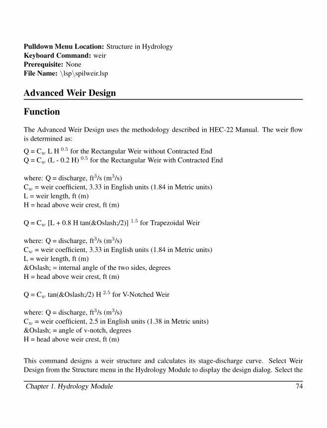
Pulldown Menu Location: Structure in Hydrology
Keyboard Command: weir
Prerequisite: None
File Name: \lsp\spilweir.lsp
Advanced Weir Design
Function
The Advanced Weir Design uses the methodology described in HEC-22 Manual. The weir flow
is determined as:
Q = Cw L H 0.5 for the Rectangular Weir without Contracted End
Q = Cw (L - 0.2 H) 0.5 for the Rectangular Weir with Contracted End
where: Q = discharge, ft3/s (m3/s)
Cw = weir coefficient, 3.33 in English units (1.84 in Metric units)
L = weir length, ft (m)
H = head above weir crest, ft (m)
Q = Cw [L + 0.8 H tan(Ø/2)] 1.5 for Trapezoidal Weir
where: Q = discharge, ft3/s (m3/s)
Cw = weir coefficient, 3.33 in English units (1.84 in Metric units)
L = weir length, ft (m)
Ø = internal angle of the two sides, degrees
H = head above weir crest, ft (m)
Q = Cw tan(Ø/2) H 2.5 for V-Notched Weir
where: Q = discharge, ft3/s (m3/s)
Cw = weir coefficient, 2.5 in English units (1.38 in Metric units)
Ø = angle of v-notch, degrees
H = head above weir crest, ft (m)
This command designs a weir structure and calculates its stage-discharge curve. Select Weir
Design from the Structure menu in the Hydrology Module to display the design dialog. Select the
Chapter 1. Hydrology Module 74

Type of the weir , Rectangular, Trapezoidal or V-notched. Enter the dimension for the weir. In
the Invert Elev box, type the absolute elevation at which the weir will be attached to a reservoir.
The attachment point is at the bottom of the weir. In the Coefficient box, type a weir coefficient
value. In the Number of Openings box, enter the number of weirs you want to combine.
In the Headwater box, type the absolute headwater surface elevation.Click on the Calculate button,
the maximum discharge and flow velocity through the weir would be computed and displayed.
Click on the Stage-Discharge Result button to display the stage-discharge curve in the Stage-
Discharge Result Dialog. This dialog allows you to write the stage-discharge data to a stage-
discharge file(.STG), and draw the stage-discharge curve on the screen. From the Stage-Discharge
Curve Draw Settings dialog , you can specify how to draw the curve.
Advanced Weir Design Dialog
Stage-Discharge Limits Dialog
Chapter 1. Hydrology Module 75

Stage-Discharge Result Dialog
Prompts
Advanced Weir Design dialog: Fill in values.
Pulldown Menu Location: Structure > Advanced Weir Design
Keyboard Command: weir
Prerequisite: None
File Name: \lsp\cntr grd.arx
Orifice Design
Function
The Orifice Design uses the methodology described in HEC-22 Manual. The orifice flow is
determined as:
Q = Co Ao (2 g Ho)0.5
where: Q = discharge, ft3/s (m3/s)
Co = orifice coefficient, unitless (0.40 - 0.60)
Ao = area of orifice, ft2 (m2)
Chapter 1. Hydrology Module 76

Ho = effective head on the orifice measured from the centroid of the opening, ft (m)
g = gravitational acceleration, 32.2 ft/s2 (9.81 m/s2)
This command designs an orifice structure and calculates its stage-discharge curve. Select
Orifice Design from the Structure menu in the Hydrology Module to display the design
dialog. Select the Section Type of the orifice, Circular or Rectangular. Enter the dimension
for the orifice. In the Invert Elev box, type the absolute elevation at which the orifice will
be attached to a reservoir. The attachment point is at the bottom of the orifice. In the Co-
efficient box, type a roughness coefficient for the orifice. The coefficient ranges from 0.4 to
0.6 (HEC-22). In the Number of Openings box, enter the number of orifices you want to combine.
In the Headwater and Tailwater boxes, type the absolute headwater surface elevation and tailwater
surface elevation respectively. Click on the Calculate button, the maximum discharge and flow
velocity through the orifice would be computed and displayed.
Click on the Stage-Discharge Result button to display the stage-discharge curve in the
Stage-Discharge Result Dialog. This dialog allows you to write the stage-discharge data to
a stage-discharge file(.STG), and draw the stage-discharge curve on the screen. From the
Stage-Discharge Curve Draw Settings dialog , you can specify how to draw the curve.
Orifice Design Dialog
Chapter 1. Hydrology Module 77

Stage-Discharge Limits Dialog
Stage-Discharge Result Dialog
Chapter 1. Hydrology Module 78

Stage-Discharge Curve Draw Settings Dialog
Prompts
Orifice Design dialog: Fill in values.
Pulldown Menu Location: Structure > Orifice Design
Keyboard Command: orifice
Prerequisite: None
File Name:\lsp\cntr grd.arx
Multiple Outlet Design
Function
Multiple Outlet Design attaches multiple outlet structures to a detention pond and computes the
stage-discharge data. All design parameters are stored in a combo outlet file (.COT). This com-
mand allows you to add, edit and remove outlet structures attached to a pond, and you can see how
different combinations of structures affect the stage-discharge calculation. There are five types of
outlet structures: culvert, drop pipe, orifice, weir and user defined stage-discharge curve. Please
refer to the documentation of Culvert Design, Drop Pipe Spillway Design, Orifice Design, Weir
Design and Input-Edit Stage-Discharge for the details.
From the Structure menu in the Hydrology Module, choose Multiple Outlet Design command to
open the design dialog. You need to specify an existing or a new combo outlet file (.COT) to load
it into the design dialog. The dialog has two edit fields: Outlet and Detention. Outlet field displays
a list of outlet structures that are attached to the detention pond. By highlighting a structure, you
can edit its parameters and see the stage-discharge calculations. In the Invert Elev box, type the
absolute elevation at which the highlighted structure will be attached. The attachment point for a
structure is at the bottom of the structure. In the Detention field, you can specify the base elevation
and the water surface elevation of the detention pond, and the total discharge will be calculated
and displayed.
Click on Add button to display the New Outlet Structure dialog. Enter the structure name and
select a structure type, then click the OK button to display the outlet design dialog for that
structure. Configure the structure in the design dialog and then click OK to exit the dialog and
come back to the main dialog, which highlights the new structure and indicates its parameters
Chapter 1. Hydrology Module 79

and the stage-discharge result.
The Edit and Remove buttons allow you to edit and remove the highlighted structure. The Stage-
Discharge Result button computes the discharges at each stage from the minimum water elevation
to the maximum, and displays the result in the Stage-Discharge Result Dialog. The Report button
reports the design parameters and the discharge results in the standard Carlson report display
window, from where the information can be edited, saved, and printed to a printer or to the screen.
The Load button allows you to load other combo outlet files (.COT) for editing. The Save and
SaveAs buttons save the current design parameters to a outlet file.
Multiple Outlet Design Dialog
New Outlet Structure Dialog
Chapter 1. Hydrology Module 80

Stage-Discharge Result Dialog
Prompts
Multiple Outlet Design dialog: Fill in values.
Pulldown Menu Location: Structure > Multiple Outlet Design
Keyboard Command: poutlet
Prerequisite: None
File Name: \lsp\cntr grd.arx
Input-Edit Stage-Storage
Function
This command allows you to define a reservoir by entering stage/storage data in four ways:
stage/storage or stage/area data, stage/contour area data, rectangular/trapezoidal pond definition
and underground pipe definition.
From the Structure > Stage-Storage menu in the Hydrology Module, choose Input-Edit Stage-
Storage to open the design dialog. Enter the pond name in the Structure Name box. There are
four Storage Methods: User Defined Storage allows you to manually enter stage-storage or stage-
area data, Irregular Shape allows you to select the contours of a surface model from a drawing,
Rectangular Shape is used to define a rectangular or trapezoidal pond and Underground Pipe is
Chapter 1. Hydrology Module 81

used to define pipe shape reservoirs. Stage-Storage Data section displays the stage-storage curve
data. Click on the Edit Detention Structure button to create/edit the stage-storage input. Load,
Save and SaveAs buttons allow you to load and save the stage-storage data.
Input-Edit Stage-Storage
User Defined Storage
In the spreadsheet, you can enter elevations and corresponding cumulative volumes, or elevations
and the corresponding areas. Before entering data, set the Storage Unit to Cumulative Volume or
Area, depending on what type of data you have. The area data represents the areas at the specified
elevation while the volume correlate to the volume between the first elevation and the current
elevation. The first entry always contains the lowest elevation in your reservoir, the cumulative
volume should be 0.0, or the area should be the area of the reservoir bottom if the Storage Unit is
area. All the elevation entries are in the increasing order. In the Base Area box, enter the area at
the lowest elevation. Insert and Delete buttons allow you to insert and deleter a row at the cursor.
Click on OK button to save the stage-storage data.
Chapter 1. Hydrology Module 82

User Defined Storage
Irregular Shape
This method allows you to define an irregular shape pond from the contour polylines of a sur-
face model, and generate the stage-storage data automatically. In order to use this method, you
must have the surface drawing open, which contains the contours that you want to use to de-
fine the reservoir. Click on the Select Pond Contours and select as many contours as you need,
the stage/storage and stage/area relationship will be then determined and displayed in the Stage-
Storage Data table, starting from the lowest elevation to the maximum. Click on OK button to
save the data.
Irregular Pond Design
Rectangular Shape
This method allows you to define a rectangular box or trapezoidal shape reservoir. Enter values
in the Top Elevation, Base Elevation, Base Length and Base Width boxes. If you want to define a
Chapter 1. Hydrology Module 83

trapezoidal shape reservoir, enter the Length Slope Ratio and Width Slope Ratio. You also need
to specify the Stage Increment. Click on OK button to save pond parameters.
Rectangular Pond Design
Underground Pipe
This method allows you to specify a reservoir as a pipe. Pipes come in circular and rectangular
shapes. Enter the pipe dimensions and the Invert Elev at which the pipe is located. Specify the
Number of Barrels and the Stage Increment. Click on OK button to save the pipe parameters.
Underground Pipe Design
Stage-Storage Curve
When you click on the Graph button, the Stage-Storage Curve dialog displays. A image is shown
for you to view the stage vs. storage, stage vs area plot for the reservoir. The graph can be plotted
into the CAD graphic by clicking on Draw button. When you click on the Draw button, the Stage-
Storage Curve Settings dialog displays from where you can define how to plot the text and graph
on screen.
Chapter 1. Hydrology Module 84

Stage-Storage Curve
Stage-Storage Curve Draw Settings
Prompts
Input-Edit Stage-Storage dialog: Fill in values.
Chapter 1. Hydrology Module 85

Pulldown Menu Location: Structure > Stage-Storage > Input-Edit Stage-Storage
Keyboard Command: edit stage store
Prerequisite: a stage-storage file (.CAP)
File Name: \lsp\cntr grd16.arx
Calculate Stage-Storage
Function
This command calculates stage-storage values for a pond that is already drawn in the drawing.
Before running this routine, the surface model for the pond must be created as a grid file with
Make 3D Grid File. A closed polyline for the perimeter of the pond is also required. It has the
option to save a stage-storage capacity file, in one of 2 forms (Carlson for readability, or Sedcad
form, for importing into Sedcad). The type of file stored is set in Configure, Hydrology Module.
Prompts
Choose Grid File
Select the .grd file that models the pond surface.
Pick the top of dam polyline: pick the closed polyline perimeter
Choose method to specify storage elevations (<Automatic>/Interval/Manual)? Manual
Range of pond elevations: 1202 to 1220
Sediment Elevation (Enter for none): 1206
Enter stage elevation (Enter for none): 1206
Enter stage elevation (Enter for none): 1210
Enter stage elevation (Enter for none): 1215
Enter stage elevation (Enter for none): 1220
Enter stage elevation (Enter for none): press Enter
Pond Storage Volumes
Chapter 1. Hydrology Module 86

Write stage-storage to file (Yes/<No>)? press Enter When saving a stage-storage capacity file,
to be drawn in the Draw Stage-Storage Curve command, it is a good idea to limit the number of
stages to a reasonable number, such as 6 to 12 stages. More than 12 will plot off the page in a long
list, unless you use the option ''Skip Every 2nd Table Entry''. If the stages are at odd intervals, the
Draw Stage-Storage Curve command will interpolate additional stages, so reducing the number
of stages used works best for plotting.
Typical Pond for Calculate Stage Storage
Pulldown Menu Location: Structure in Hydrology
Keyboard Command: postpond
Prerequisite: Surface entities that model the pond
File Name: \lsp\makegrid.arx
Draw Stage-Storage Curve
Function
This routine draws a pond stage storage curve with pond elevation on the vertical axis and
acre-feet of storage on the horizontal axis. It will plot and label the emergency spillway, principal
spillway and cleanout levels and will produce a table of storage data. The program will read and
write a .CAP file of pond storage, based on areas at each stage or elevation. CAP files (short for
''capacity'') are made by Bench Pond Design, Valley Pond Design, Rectangular Pond Design,
Calculate Stage Storage and by the Stage Storage Curve program itself. These programs output
Chapter 1. Hydrology Module 87

two types of CAP files, one which is read by SEDCAD, a popular hydrology and sedimentology
program, and another which is a simple comma-delimited file for easy viewing in spreadsheets
or text editors.
In addition to file-based inputs, the user can enter pond dimensions directly by length-width, area
at each stage, or volume at each stage. The above drawing was created by the entry of widths
and lengths at increasing elevation, entered within the routine itself. Also shown at the bottom is
the default certification, obtained by clicking on the certification option. All text is editable. If
stage-storage curves are loaded from file, which contains only volumes at different stages, then
the width and length columns are filled in as ''N/A'' (not applicable). Since volume-based entry
does not include area information, no CAP files are stored with this option. However, the curves
plot in all cases. Plots are sized to fit on 8.5 x 11 sheets at the selected scale for plotting. They
are particularly suited for permit applications, so the program will prompt for permit number and
page.
Prompts
The program is dialog-driven. The first dialog controls file loading and some pre-calculation
options, and is shown below:
Chapter 1. Hydrology Module 88

In this case we have loaded a stage-storage curve from a stored capacity file. The program will
automatically display the top of structure. If your goal is to set the emergency spillway at an
elevation with storage 5.5 acre-feet, you can enter the storage in the lower left and calculate
the appropriate elevation. You can also compute permanent pool elevations by entering runoff
quantities. A total runoff of 3.5 acre feet, subtracted from the acre-feet at the principal spillway,
will set the recommended elevation of the ''clean out level''. If the pond silts up above that level,
then the silt needs to be removed. In Kentucky, for example, the minimum vertical separation
between principal spillway and clean out level is 1.5 feet.
If you choose to manually enter the pond area, dimensions or volume at increasing stages
(elevations), then all the options in the lower portion of the dialog ''ghost'' and are not available,
since the pond characteristics are not yet known. Then prompting appears as shown below:
Prompts
Input (A)rea, Length/Width (D)imensions or <V>olume: D
Stage No. 1
Elevation: 940
Width: 20
Length: 60
Chapter 1. Hydrology Module 89

<Enter> for more, (R) to Revise, (E) to exit entry: If you made a mistake, you could enter R
and then enter a revised Elevation, Width and Length. Otherwise, press Enter to continue.
Stage No. 2
Elevation: 945
Width: 30
Length: 70
<Enter> for more, (R) to Revise, (E) to exit entry: press Enter
Stage No. 3
Elevation <950.00>: The program defaults to the last interval.
Width: 40
Length: 80
<Enter> for more, (R) to Revise, (E) to exit entry: E to exit
A table appears, similar to the following:
Elev Width Length Area Interval Avg. Area Inc. Vol Acc. Vol Stage
(Ft) (Ft) (Ft) (Acre) (Ft) (Acre) (Acre Ft) (Acre Ft)
-----------------------------------------------------------------------------
940 20.0 60.0 0.028 0.00 0.028 0.000 0.000 0.00
945 30.0 70.0 0.048 5.00 0.038 0.189 0.189 5.00
950 40.0 80.0 0.073 5.00 0.061 0.304 0.494 10.00
Areas are in acres. If the area method of entry were chosen instead, the user would have been
prompted for area at each elevation (stage), and the summary table would be blank under the
width and length columns. Similarly, if entry was by volume (in cubic feet), all width, length and
area columns would be blank.
Calculate Storage or Elevation Points (y/<n>): y
Known (E)levation or known <S>torage:
Storage (e.g. 0.2 or %60 for 60% of total): %60
Storage: 0.30 Elevation: 946.759
Calculate Storage or Elevation Points (y/<n>): press Enter This allows you to move on. The
advantage of this option is the ability to find exact spillway and cleanout levels by experimenting
with needed storages or desired elevations. For example, sediment cleanout levels are often set at
60% of total storage, which would be in this case 946.76.
Elevation of Top of Structure: 950
Elevation of Emergency Spillway: 948.5
Elevation of Principal Spillway (Enter if same): press Enter
Elevation of Cleanout Level: 946.76
Chapter 1. Hydrology Module 90

Is Above Data OK (<y>/n): press Enter n leads to re-entry of above 4 items
Regardless of whether the stage-storage information was hand-entered or loaded from a capacity
file, you are in all cases led to the next dialog, which governs the drawing and labeling of the
stage-storage curve graph and text:
Note that it is often beneficial to ''skip every 2nd table entry'', since the table of text for each
stage may exceed the space alloted to it. You can also plot a ''Stage-Area Curve'' as well as a
Stage-Storage Curve, with the Stage-Area horizontal access scale information plotted on the top
of the graph.
A business address or typed-in certification can be entered here as well.
Prompts
Pick Starting Position: pick lower left corner of stage storage curve on screen
Company Name: Maysville Survey & Engineering
Address Line 1: 105 W. 2nd Street
Address Line 2: Maysville, KY 41056
Address Line 3:
Store Pond Capacity File (y/<n>): y This prompt appears if you hand-enter stage-storage in-
formation without the routine and is followed by the normal store file dialog.
Chapter 1. Hydrology Module 91

Note that if Drawing Setup is set to metric, the stage-storage curve is calculated in cubic meters
and all entries are in meters. The final result of a typical combined Stage-Storage and Stage-Area
plot is shown below:
Pulldown Menu Locations: Structure in Hydrology, Surface in Mining
Keyboard Command: stage
Prerequisite: None
File Name: \lsp\stage.lsp
Input-Edit Stage-Discharge
Function
This command allows you to manually input and edit the discharge data at specific elevations. A
rating curve is created between the minimum and maximum elevations. Insert Row and Delete
Row buttons insert and delete rows at the cursor. Load, Save and SaveAs buttons allow you to
load and save the stage-discharge data. Click on the Graph button to open the Stage-Discharge
Curve dialog to view the stage-discharge data. After viewing the data, you can plot the graph into
the CAD graphic by clicking on Draw button. When you click on the Draw button, the Stage-
Chapter 1. Hydrology Module 92

Discharge Curve Settings dialog displays from where you can define how to plot the text and
graph on screen.
Input-Edit Stage-Discharge
Stage-Discharge Curve
Chapter 1. Hydrology Module 93

Stage-Discharge Curve Draw Settings
Prompts
Input-Edit Stage-Discharge dialog: Fill in values.
Pulldown Menu Location: Structure > Stage-Discharge > Input-Edit Stage-Discharge
Keyboard Command: edit stage discharge
Prerequisite: a stage-discharge file (.STG)
File Name: \lsp\cntr grd16.arx
Draw Stage-Discharge Graph
Function
This program draws a stage-discharge graph with the stage (water elevation) on the Y-axis and
the discharge on the X-axis. The data to graph is read from a stage-discharge (.stg) file which can
be created by several routines including Design Channel, Drop Spillway, etc.
First you are prompted to select a STG file to draw. Then the program asks for the ending dis-
charge for the graph which defaults to the highest discharge in the file. Next this dialog is dis-
played to enter the graph scale and intervals. The height of the annotation equals the horizontal
scale times the Axis Text Scaler.
Chapter 1. Hydrology Module 94

Pulldown Menu Location: Structure in Hydrology
Keyboard Command: stage2
Prerequisite: Stage-Discharge file (.stg)
File Names: \lsp\hydrogrf.lsp, \lsp\hydro.dcl
Report Stage-Discharge
Function
Chapter 1. Hydrology Module 95
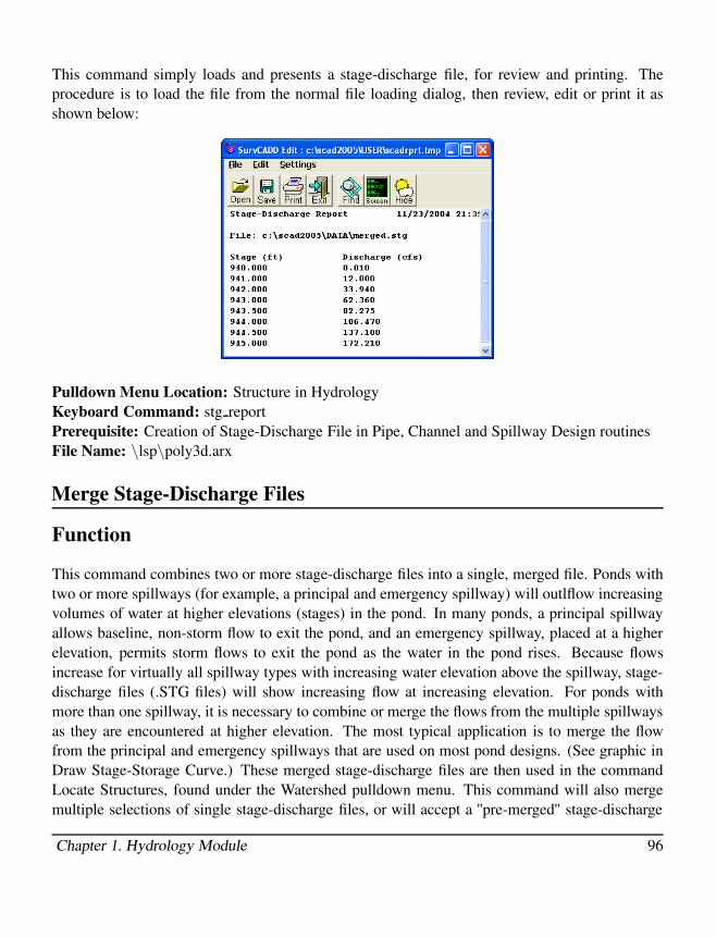
This command simply loads and presents a stage-discharge file, for review and printing. The
procedure is to load the file from the normal file loading dialog, then review, edit or print it as
shown below:
Pulldown Menu Location: Structure in Hydrology
Keyboard Command: stg report
Prerequisite: Creation of Stage-Discharge File in Pipe, Channel and Spillway Design routines
File Name: \lsp\poly3d.arx
Merge Stage-Discharge Files
Function
This command combines two or more stage-discharge files into a single, merged file. Ponds with
two or more spillways (for example, a principal and emergency spillway) will outlflow increasing
volumes of water at higher elevations (stages) in the pond. In many ponds, a principal spillway
allows baseline, non-storm flow to exit the pond, and an emergency spillway, placed at a higher
elevation, permits storm flows to exit the pond as the water in the pond rises. Because flows
increase for virtually all spillway types with increasing water elevation above the spillway, stage-
discharge files (.STG files) will show increasing flow at increasing elevation. For ponds with
more than one spillway, it is necessary to combine or merge the flows from the multiple spillways
as they are encountered at higher elevation. The most typical application is to merge the flow
from the principal and emergency spillways that are used on most pond designs. (See graphic in
Draw Stage-Storage Curve.) These merged stage-discharge files are then used in the command
Locate Structures, found under the Watershed pulldown menu. This command will also merge
multiple selections of single stage-discharge files, or will accept a ''pre-merged'' stage-discharge
Chapter 1. Hydrology Module 96

file. In combination with the pond stage-storage files, the structures in a watershed layout will be
used to compute hydrographs and determine the impact of pond placement and spillway design
on reducing storm flows.
Prompts
The command is dialog-driven, in this order:
First Stage-Discharge File to Merge. (It is recommended to load the lowest elevation spillway
file, typically the principal spillway stage-discharge file.)
Next Stage-Discharge File to Merge. (Here you would typically load the emergency spillway
stage-discharge file.)
Merge Another Stage-Discharge File? Yes/No. Click Yes if there is another stage-discharge
file, otherwise click No.
Choose the Output Stage-Discharge File. Name the ouput stage-discharge file.
Pulldown Menu Location: Structure in Hydrology
Keyboard Command: merge stg
Prerequisite: Spillway design routines that create Stage-Discharge Files, such as Drop Pipe Spill-
way Design, Pond Weir Spillway Design, Open Channel (Manning's Eq) and Pipe Culvert Design.
Channel Design - NonErodible Mannings Equation
Function
This will compute channel depth, flow and velocity based on channel parameters such as side
slopes, base dimensions and Manning's n value. It handles triangular, trapezoidal , rectangular
and irregular channels. Entry of a depth leads to calculation of flow and velocity. Entry of one
of the other items (flow or velocity) will lead to calculation of the remaining items. In addition
to functioning as a channel calculator, the program will output a typical section or detail of the
channel as well as a report of the channel output. The routine also works in metric units. It
applies to non-erodible channels, primarily. The user can select to output an ASCII file report
of the channel input and output values as well as a standard detail shown below for the above
example.
Prompts
When the routine is selected, the dialog box shown below appears. Select, for example, a trape-
zoidal channel, equal sides, with side slopes of 3 (for 3:1) and a base dimension of 16. Enter the
Manning's n value and channel slope as shown. Note that 0.1, in English units, means 0.1 foot
Chapter 1. Hydrology Module 97

drop per 100 foot of length. Then at the lower right, plug a value of 4.5 for the depth. This will
calculate a flow of 862 CFS and a velocity of 6.5 fps, as shown below. If the channel is divided
into two types of materials (paved lower portions and vegetated upper portion), you can specify a
second Manning's n for the upper banks, as shown in the dialog.
To use the routine as a calculator, enter the known value in the lower right area of the dialog (flow,
depth, or velocity), then press enter while still in the entered item. The other two items are then
calculated. Note that the routine will default to the last values used during the current Carlson
work session, and will capture the flow values calculated in Water Runoff under the Watershed
Pull-down. When entering the Manning's n value, a table of n values can be brought up and an
appropriate Manning's selected. Among the output options is ''Draw Channel Detail'', which will
draw and annotate as shown below. Since Open Channels are often used as emergency spillways,
the Write Stage/Discharge File will output an .STG file for use in the command Locate Structure
under Watershed, for pond design and storm routing and hydrograph calculations.
Chapter 1. Hydrology Module 98

Pulldown Menu Location: Structure in Hydrology
Keyboard Command: channel1
Prerequisite: Use Drawing Setup to activate Metric or English outputs. If English is configured,
the formula v=(1.486/n)(Rˆ2/3)(sˆ1/2) is used, where n is the Manning's value, R is the water
cross section divided by the wetted perimeter and s is the slope ratio. If Metric is configured, the
formula becomes v=(1.0/n)(Rˆ2/3)(sˆ1/2) and outputs are in meters. To test metric, set to metric
in Drawing Setup. Then for a rectangular, concrete open channel of 12.0 meters width, slope of
0.28%, Manning's n of 0.013 and depth of 2.5 meters, you should compute a velocity of 5.94 m/s
and Q (flow) of 178 cubic meters/second.
File Names: \lsp\channel.lsp, \lsp\hydro.dcl
Channel Design - Erodible Mannings Equation
Function
This command uses the same Manning's equations as non-erodible channel design. In this case,
the discharge and velocity are known. The velocity must be less than a maximum to prevent
erosion. The program calculates the channel dimensions that meet the requirements.
First choose the channel and water type. Then either enter the Manning's n, velocity, and tractive
force or select them from a table of channel types by clicking Select from Table. Also fill in the
slope and discharge. Finally, choose either Calc Base or Calc Ratios to compute the channel di-
mensions. The Standard Parameters are used in drawing the channel detail. When OK is selected,
the routine ends and the channel is drawn if Draw Channel Detail is checked.
Chapter 1. Hydrology Module 99

When choosing Calc Base or Calc Ratios, there will be a message Error: unable to solve these
parameters on the top line if the design parameters never reach erosion conditions for any chan-
nel dimension. Consider an extreme error case with a discharge of 1 cfs, a slope of 0.1%, and a
velocity of 5.0 fps. There are no dimensions that meet these requirements. So, for this case, the
channel dimensions can be set anyway to avoid erosion.
Pulldown Menu Location: Structure in Hydrology
Keyboard Command: channel2
Prerequisite: None
File Names: \lsp\chan erd.lsp, \lsp\hydro.dcl
Pipe Culvert Design
Function
A culvert is a hydraulically short conduit, which can be used to convey stream flow underground
through a roadway embankment or other flow obstructions, or used as an outlet structure attached
to a detention pond. Culverts come in circular and rectangular cross sections, and concrete, cor-
rugated steel, aluminum and plastic materials.
The hydraulics of a culvert are complex since several flow control types may exist. The methods
Chapter 1. Hydrology Module 100

that Pipe Culvert Design uses are from FHWA Hydraulic Design Series No. 5 (HDS-5), Hy-
draulic Design of Highway Culverts. There are two flow controls: inlet control and outlet control.
Under inlet control, the culvert's entrance characteristics determine it's capacity, and the culvert is
capable of conveying a greater discharge than the inlet will accept. With outlet control, the inlet
can accept more flow than the culvert can carry because of the head loss due to the friction along
the barrel or the high tailwater elevation. Furthermore, because culverts are generally not long
enough to achieve uniform flow, the flow profile inside is often gradually or rapidly varied flow.
In Pipe Culvert Design, bother inlet control and outlet control calculations are performed, along
with the gradually varied flow analysis. The worst-performing control condition is then used to
evaluate the proposed design, i.e. the greater of the inlet control headwater and the outlet control
headwater is the controlling headwater. Please refer to HDS-5 for details.
From the Structure menu in the Hydrology Module, choose Pipe Culvert Design to display the
design dialog. Click on Load button to load an existing culvert file to view or modify it, or a new
file to start a fresh design. From the Solve For list, select the value that you want to calculate.
The available values are: Discharge, Headwater and Size.
Culvert Design
Culvert Section
Chapter 1. Hydrology Module 101

From the Shape list, select the type of culvert that you want to define. The available shapes are
Circular and Box. From the Material list, select the material for the culvert, the available options
are Concrete or CMP/Aluminum. If you don't solve for the culvert size, enter the values in the
Diameter box or Height and Width boxes depending on the culvert shape. In the Manning's n
box, type a Manning's n roughness coefficient for the culvert. You can also click on Select button
to select a coefficient from the Manning' n Library. Please refer to Pipe Manning's N Library for
defining Manning's n values. In the Number of Barrels box, enter the number of barrels for the
culvert.
Culvert Inlet
The Inlet list contains the different inlet types available for the current culvert shape. It updates
with different culvert shape that is chosen. All the inlet types are specified in HDS-5. Ke is the
entrance loss coefficient, which is depending on the culvert shapes and inlet types. It'll update
with different chosen culvert shape and inlet type, you can also type the value in the box.
Culvert Inverts
Inlet Invert is the elevation of the bottom of the culvert at the upstream end, while Outlet Invert
is the elevation of the bottom of the culvert at the downstream end. In the Length box, enter the
true culvert pipe length. The culvert slope will be calculated after entering the above three values
and displayed in the Slope box. You can also change the outlet invert by entering a slope for the
culvert.
Calculation
In the Discharge box, enter the rate of flow in the culvert. In the Headwater Elev box, enter the
water surface elevation at the upstream end of the culvert. If you are solving for either discharge
or headwater, the corresponding box will be disabled. In the Tailwater Elev box, enter the water
surface elevation at the downstream end. Section Size Library allows you to specify as many
as available pipe sizes for solving for culvert size. After the hydraulic calculation, the smallest,
large enough, available pipe size will be chosen. Please refer to the Pipe Size Library command
for defining pipe sizes. Click on Solve button, depending on Solve For selection, the headwater,
discharge, culvert size are calculated and displayed in the dialog correspondingly. The Outlet
Velocity and Flow Depth are calculated and shown, and the Control Type is also illustrated.
Outputs
Click on the Stage-Discharge Result button to display the stage-discharge curve in the Stage-
Discharge Result Dialog. From this dialog, you can view the stage-discharge curve, write the
Chapter 1. Hydrology Module 102

result to a stage-discharge file(.STG), and draw the graph into the CAD graphic. When you click
on the Draw button, the Stage-Discharge Curve Settings dialog displays from where you can
define how to plot the text and graph on screen.
Stage-Discharge Limits
Stage-Discharge Dialog
Click on Generate Report button, the program will present a report screen that contains detailed
information regarding the design parameters and the calculations. The report window provides
the options of printing, drawing the report in AutoCAD or storing the report to a file. Shown
below is an example.
Chapter 1. Hydrology Module 103

Culvert Report
A rating table presents the discharge-headwater relationship in the tabular form. It can be dis-
played in a Microsoft spreadsheet or a standard report. Click on Generate Rating Table button to
open Rating Limits dialog. In the Variant list, select the independent variable. The available vari-
ables are Discharge and Headwater. Enter data in the Minimum, Maximum and Increment boxes.
Enter the Tailwater Elev and select the decimal setting from the Decimals list. When you finish
entering data, click on OK button to calculate the rating table. A rating table example is shown
below in the standard report format. The first column Discharge is an independent variable, and
the other columns are computed variables.
Culvert Rating Table Limits
Chapter 1. Hydrology Module 104

Culvert Rating Table in Report Format
Generate Sedcad File button produces a file with a .CVT extension that can be used as one of
the building blocks for the SedCad Program ( a third hydrology and sedementology stand-alone
software package). The file is identical to what is produced within SedCad by its utilities program.
Draw Pipe Detail button plots a fully annotated standard detail, with user-controlled inlet and
outlet slope entries and scaling.
Draw Pipe Detail Settings
Prompts
Chapter 1. Hydrology Module 105

Culvert Design dialog: Fill in values
Pulldown Menu Location: Structure > Pipe Culvert Design
Keyboard Command: culvert
Prerequisite: a culvert file
File Name: \lsp\cntr grd16.arx
Sewer Pipe Design: Individual
Function
This command calculates the travel time, flow depth, and velocity for a section of pipe. It cal-
culates for one pipe section using the dialog shown here. Pipe sections can be entered as up-
stream/downstream stations and elevations, or as length and slope. Clicking Calculate will give
you Design Output data based upon your input. Follow up Calculate by clicking Report, which
will give you the Standard Report Viewer. Even after reviewing the information in the viewer and
clicking on the viewers' Exit button, or its other output buttons, you still have the opportunity to
change your original dialog box entries. This is because the command cycles from the viewer
back into the dialog box for modifications. The Draw Pipe button draws the pipe details on the
screen. The Exit within the dialog ends the command.
Sewer Pipe Design: Individual
Prompts
Chapter 1. Hydrology Module 106

Sewer Pipe Design dialog Fill in variables. Click Calculate, then click Report.
Report results from the Standard Report Viewer:
Sewer Design
Upstream Station: 0.000 Invert Elev: 395.400
Downstream Station: 400.000 Invert Elev: 390.400
Flow Rate (GPM): 50.00
Pipe Diameter (in): 8.00
Manning's n: 0.020
Length (ft): 400.00
Slope (ft/ft): 0.0125
Travel Time (min): 3.86
Flow Depth (in): 1.92
Velocity (fps): 1.73
Pulldown Menu Location: Structure > Sewer Pipe Design > Individual
Keyboard Command: swrpipe
Prerequisite: None
File Name: \lsp\swrpipe.lsp
Sewer Pipe Design: Sewer Network Segment
Function
This command reads a sewer network and displays every pipe segment in the Sewer Pipe Design
dialog. From the Structure > Sewer Pipe Design menu in the Hydrology Module, select Sewer
Network Segment. The function reads a sewer network file, conducts the hydraulic calculations
and displays pipe parameters and results in the dialog. Pipes list contains all pipe segments, you
can select any one of them to display its data. Return Period list allows you to specify different
rainfall conditions for different hydraulic results. The pipe parameters are shown in the middle
part of the dialog, and the results are shown in the bottom table. Load button loads another sewer
network file, Report button reports current pipe information to the standard Carlson report, and
Report All button reports all pipe data to the standard report.
Chapter 1. Hydrology Module 107

Sewer Pipe Design: Sewer Network Segment
Prompts
Sewer Network Segment dialog: Fill in values.
Pulldown Menu Location: Structure > Sewer Pipe Design > Sewer Network Segment
Keyboard Command: swrpipe3
Prerequisite: a sewer file (.SEW), ...\USER\RainLib.dta, ...\USER\inlet.dta,
...\USER\pipesize.dta (mpipesize.dta in Metric unit)
File Name: \lsp\cntr grd16.arx
Sewer Pipe Design: Read Profile
Function
This command calculates the travel time, flow depth, and velocity for a section of pipe. It
reads the stations and elevations of a sewer or pipe profile (.PRO) created by the Design
Sewer/Pipe Profile command in the Civil Design module. Pipe sections can be entered as
upstream/downstream stations and elevations or as length and slope.
Prompts
Chapter 1. Hydrology Module 108
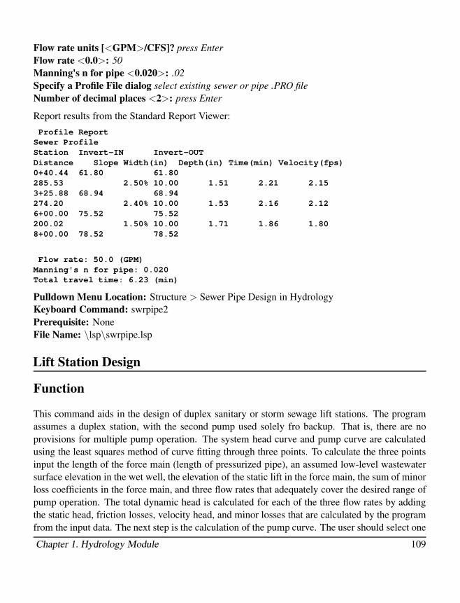
Flow rate units [<GPM>/CFS]? press Enter
Flow rate <0.0>: 50
Manning's n for pipe <0.020>: .02
Specify a Profile File dialog select existing sewer or pipe .PRO file
Number of decimal places <2>: press Enter
Report results from the Standard Report Viewer:
Profile Report
Sewer Profile
Station Invert-IN Invert-OUT
Distance Slope Width(in) Depth(in) Time(min) Velocity(fps)
0+40.44 61.80 61.80
285.53 2.50% 10.00 1.51 2.21 2.15
3+25.88 68.94 68.94
274.20 2.40% 10.00 1.53 2.16 2.12
6+00.00 75.52 75.52
200.02 1.50% 10.00 1.71 1.86 1.80
8+00.00 78.52 78.52
Flow rate: 50.0 (GPM)
Manning's n for pipe: 0.020
Total travel time: 6.23 (min)
Pulldown Menu Location: Structure > Sewer Pipe Design in Hydrology
Keyboard Command: swrpipe2
Prerequisite: None
File Name: \lsp\swrpipe.lsp
Lift Station Design
Function
This command aids in the design of duplex sanitary or storm sewage lift stations. The program
assumes a duplex station, with the second pump used solely fro backup. That is, there are no
provisions for multiple pump operation. The system head curve and pump curve are calculated
using the least squares method of curve fitting through three points. To calculate the three points
input the length of the force main (length of pressurized pipe), an assumed low-level wastewater
surface elevation in the wet well, the elevation of the static lift in the force main, the sum of minor
loss coefficients in the force main, and three flow rates that adequately cover the desired range of
pump operation. The total dynamic head is calculated for each of the three flow rates by adding
the static head, friction losses, velocity head, and minor losses that are calculated by the program
from the input data. The next step is the calculation of the pump curve. The user should select one
Chapter 1. Hydrology Module 109

or more pumps from a manufacturer's catalog that will produce the desired operating conditions.
The input data consists of the pump shutoff head (flow rate equal to zero), a head and flow rate
near the desired operating point, and a head and flow rate beyond said operating point of the pump
curve.
Chapter 1. Hydrology Module 110

The system head curve and the pump curve are then intersected to produce preliminary operating
point results. If the user is not happy with the results, click the Edit Input Values button and
change any of the parameters. When the user attains the desired results then proceed with the wet
well design by clicking OK.
Input for the wet well design includes type of wet well, wet well dimensions, invert elevation of
the lowest line entering the wet well, and minimum wastewater depth in the wet well (usually
specified by the pump maker). The lead pump's wet well volume is calculated using a formula
from Metcalf & Eddy's Wastewater Engineering: Collection and Pumping of Wastewater: V =
CT/4, where V equals required volume in gallons, C equals pump capacity (GPM), and T equals
minimum time in minutes of one pumping cycle. After wet well design the program assigns a
new low level wastewater surface elevation in the wet well, and then recalculates the system
head curve and final operating point. At this point the user may change any or all of the input
parameters. If no changes are needed then click OK to show the Final Results report.
Chapter 1. Hydrology Module 111

Pulldown Menu Location: Structure in Hydrology
Chapter 1. Hydrology Module 112

Keyboard Command: LIFTSTA
Prerequisite: None
File Names:\lsp\liftstat.lsp, \lsp\liftstat.dcl
Network Menu
The Network pull-down menu has commands for layout and analysis of storm sewer networks.
Sewer Network Settings
Function
This command sets the options for how to update the sewer network if the reference surface
or centerline changes. Each structure has the option to assign a reference centerline and the
structure will record the station and offset from this centerline. When the reference centerline
of a structure changes, the structure can be moved to the position of the recorded station and
offset along the modified centerline. If the reference surface changes, the structure rim elevation
can be updated and there are two options for updating the invert elevation. One method is to
hold the structure depth and change the invert elevation. The other method is to hold the invert
elevation and change the depth. The structure updates for reference surface or centerline changes
can be turned off, prompted or automatic. If the updates are turned off, then the Check Reference
Centerlines and Surface can be used to compare the sewer network with the references file. Also
Chapter 1. Hydrology Module 113

the structures can be updated manually with Edit Sewer Structure. If the update is set to prompt,
then each time that the reference files are changed, the program will prompt whether to update
the structures. If the update is set to automatic, then the structures will update along with the
labels.
Pulldown Menu Location: Network
Keyboard Command: setconfig
Prerequisite: none
File Name: \lsp\cntr grd.arx
Set Sewer File
Function
This command sets a sewer network file as the current file. The other sewer network commands
will reference this file. Either a new file can be created or an existing sewer file can be modified.
The sewer network file stores all the sewer structure data (elevation, flow) and all the network
connection data (slopes, pipe sizes). This file has a .sew file extension.
Pulldown Menu Location: Network
Keyboard Command: setswr
Prerequisite: none
File Name: \lsp\pswrfile.lsp
Set Surface File
Function
Chapter 1. Hydrology Module 114

Use this command to set the grid or triangulation file to be used to compute sewer manhole surface
elevations and minimum cover along pipe lengths, within the Sewer Network commands, and in
particular the command Create Sewer Structure. A dialog will appear requesting the name of the
surface file to be used.
Pulldown Menu Location: Network
Keyboard Command: setgrd
Prerequisite: None
File Name: \lsp\hydro1.lsp
Plan View Label Settings
Function
This command sets the drawing format for sewer pipeline and inlet/manhole annotations drawn
for the sewer network. The settings are entered in a dialog with tabs for Structure Labels, Pipe
Labels and General Settings.
Shown below is the manhole or inlet name, along with rim elevation, invert elevation and the
Chapter 1. Hydrology Module 115

labelling of the sewer pipe itself.
Under Structure Labels, you can choose whether to label the structure name, rim elevation,
invert-in elevation or invert-out elevation. There are settings for the prefix and suffix for each
of these labels. The invert elevations can be positioned either above the structure or along the
associated pipe direction. The Add Quadrant option adds the bearing quadrant of the associated
pipe direction to the invert label prefix. The option to Use Structure Data Table will put the labels
is a block as shown below instead of regular text entities. There are settings for the size of the
block columes and the block label justification.
Chapter 1. Hydrology Module 116
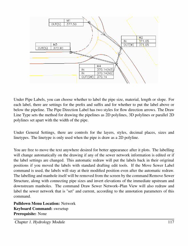
Under Pipe Labels, you can choose whether to label the pipe size, material, length or slope. For
each label, there are settings for the prefix and suffix and for whether to put the label above or
below the pipeline. The Pipe Direction Label has two styles for flow direction arrows. The Draw
Line Type sets the method for drawing the pipelines as 2D polylines, 3D polylines or parallel 2D
polylines set apart with the width of the pipe.
Under General Settings, there are controls for the layers, styles, decimal places, sizes and
linetypes. The linetype is only used when the pipe is draw as a 2D polyline.
You are free to move the text anywhere desired for better appearance after it plots. The labelling
will change automatically on the drawing if any of the sewer network information is edited or if
the label settings are changed. This automatic redraw will put the labels back in their origrinal
positions if you moved the labels with standard drafting edit tools. If the Move Sewer Label
command is used, the labels will stay at their modified position even after the automatic redraw.
The labelling and manhole itself will be removed from the screen by the command Remove Sewer
Structure, along with connecting pipe sizes and invert elevations of the immediate upstream and
downstream manholes. The command Draw Sewer Network–Plan View will also redraw and
label the sewer network that is ''set'' and current, according to the annotation parameters of this
command.
Pulldown Menu Location: Network
Keyboard Command: swrsetup
Prerequisite: None
Chapter 1. Hydrology Module 117

File Name: \lsp\cntr grd.arx
Save Sewer Network File
Function
This routine re-saves the current sewer network file in another name, which can act as a backup
file or ''snapshot'' of the sewer network design at a certain point in time. The file can be re-loaded
later and re-used.
Pulldown Menu Location: Network
Keyboard Command: save sewer
Prerequisite: Sewer network (.SEW) file
File Name: \lsp\scadutil.arx
Import Haestad Network
Function
This routine converts Haestad files into Carlson sewer files. Haestad sewer network files have
fourteen pieces of information in an ASCII text file. Unfortunately, they do not contain two-
dimensional coordinates of the manholes locations. Therefore, the routine must assume locations
along some arbitrary datum. Examine the example output below. The program searches for the
longest path along the sewer network, and places it on the X axis. The next longest set(s) of
network traces branch from the longest path. The process is repeated until the last upstream
manhole on the network tree branches is encountered. While true coordinate locations of the
manholes is unknown, additional hydraulic analysis of the system can be made on this Carlson
pseudo-layout.
Chapter 1. Hydrology Module 118

Pulldown Menu Location: Network->Sewet Network Setup
Keyboard Command: ha2csnet
Prerequisite: Haestad file
File Names: \lsp\ha2csnet.lsp, \exec\ha2csnet.exe
Rainfall Library
Function
Rainfall is the source of the ground runoff. Along with the watershed conditions, the rainfall that
neither infiltrates nor gets trapped in low areas and depressions contributes to the direct surface
runoff, upon which the storm drainage system design is based.
The Rainfall Library use IDF curves to provide average rainfall intensity data for particular storm
events. With a known rainfall duration and frequency, an intensity is calculated via the IDF curve
and applied to the Rational Method to obtain the peak flow for designing the sewer network.
There are five methods to input rainfall data: TP-40 rainfall map, Hydro-35 rainfall map,
rainfall accumulation, rainfall intensity and IDF equation coefficients. Rainfall maps provided
by government organizations are practical rainfall data resources for engineering design. TP-40
maps show precipitation depths in the US for storm durations from 1 hour to 24 hours and for
recurrence intervals from 1 to 100 year. Hydro-35 maps are for the central and eastern US, and
provide rainfall data for durations as short as 5 minutes. Please refer to HEC-12 for details on
methodology for computing IDF curves from rainmaps. In addition to TP-40 and Hydro-35
method, you can input rainfall accumulations or intensities at various storm durations to define
IDF curves. If you already have the IDF equation coefficients calculated, you can enter the
Chapter 1. Hydrology Module 119

coefficients directly to define the IDF curves. The IDF curves are interpolated linearly between
the data points.
The IDF equation for a given return period is defined as follows. The coefficients A, B and M are
calculated by log-log regression of the rainfall intensity and (t + B).
I = A / (t + B)M
where: I = rainfall intensity (in/hr, or mm/hr in metric)
A, B, M = equation coefficients for a given return period
t = rainfall duration (min.)
The Rainfall Library stores rainfall data in a library file under the ...\USER folder and is available
for all projects. From the Network > Sewer Network Libraries menu in the Hydrology Module,
select the Rainfall Library to open the library dialog to edit rainfall data. The dialog lists all
rainfall entries by their ID and their input/edit method. New button creates a new rainfall through
one of the five methods: TP-40, Hydra-35, Rainfall Accumulation, Rainfall Intensity and IDF
Equation Coefficients. Edit button allows you to modify an existing rainfall, and the Delete button
removes the highlighted rainfall from the library. Load and SaveAs buttons allow you to load and
save the rainfall data.
Rainfall Library Dialog
Chapter 1. Hydrology Module 120
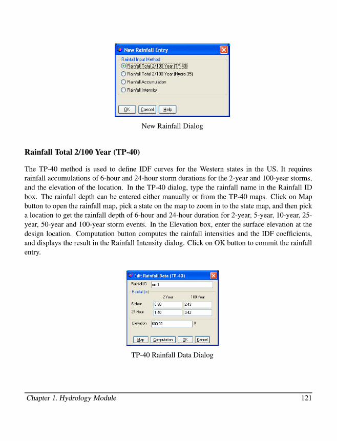
New Rainfall Dialog
Rainfall Total 2/100 Year (TP-40)
The TP-40 method is used to define IDF curves for the Western states in the US. It requires
rainfall accumulations of 6-hour and 24-hour storm durations for the 2-year and 100-year storms,
and the elevation of the location. In the TP-40 dialog, type the rainfall name in the Rainfall ID
box. The rainfall depth can be entered either manually or from the TP-40 maps. Click on Map
button to open the rainfall map, pick a state on the map to zoom in to the state map, and then pick
a location to get the rainfall depth of 6-hour and 24-hour duration for 2-year, 5-year, 10-year, 25-
year, 50-year and 100-year storm events. In the Elevation box, enter the surface elevation at the
design location. Computation button computes the rainfall intensities and the IDF coefficients,
and displays the result in the Rainfall Intensity dialog. Click on OK button to commit the rainfall
entry.
TP-40 Rainfall Data Dialog
Chapter 1. Hydrology Module 121

TP-40 Rainfall Map
Rainfall Intensity Results
Rainfall Total 2/100 Year (Hydro-35)
The Hydro-35 method is used to define IDF curves for the Central and Eastern states in the US.
Chapter 1. Hydrology Module 122

It requires rainfall accumulations of 5-min, 15-min and 60-min storm durations for the 2-year
and 100-year storms. In the Hydro-35 dialog, type the rainfall name in the Rainfall ID box. The
rainfall depth can be entered either manually or from the Hydro-35 maps. Click on Map button
to open the rainfall map, pick a state on the map to zoom in to the state map, and then pick a
location to get the rainfall depth. Computation button computes the rainfall intensities and the
IDF coefficients at 2-year, 5-year, 10-year, 25-year, 50-year and 100-year return periods, and
displays the result in the Rainfall Intensity dialog. Click on OK button to commit the rainfall
entry.
Hydro-35 Rainfall Data
Hydro-35 Rainfall Map
Rainfall Accumulation
This method allows you to enter the rainfall accumulations of various durations for 2-year, 5-year,
Chapter 1. Hydrology Module 123

10-year, 25-year, 50-year and 100-year return periods for computing the IDF curves. Add a Dura-
tion button adds new duration entry to the spreadsheet. For the accuracy, three or more durations
are required. Delete a Duration button deletes the highlighted duration entry. Computation button
computes the rainfall intensities and the IDF coefficients, and displays the result in the Rainfall
Intensity dialog. Click on OK button to commit the rainfall entry.
Customed Rainfall Accumulations
New Duration Entry
Rainfall Intensity
This method allows you to enter the rainfall intensities of various durations for 2-year, 5-year, 10-
year, 25-year, 50-year and 100-year return periods for computing the IDF curves. Add a Duration
button adds new duration entry to the spreadsheet. For the accuracy, three or more durations are
required. Delete a Duration button deletes the highlighted duration entry. Computation button
computes the rainfall intensities and the IDF coefficients, and displays the result in the Rainfall
Intensity dialog. Click on OK button to commit the rainfall entry.
Chapter 1. Hydrology Module 124

Customed Rainfall Intensities
Enter IDF Equation Coefficients
When you have the coefficients calculated, you can use this method to enter the coefficients
to obtain the actual IDF curve equation. In the following spreadsheet dialog, enter the known
coefficients A, B and M to create the IDF equation. Computation button computes the rainfall
intensities and displays the result in the Rainfall Intensity dialog. Click on OK button to commit
the rainfall entry.
IDF Equation Coefficients
Prompts
Rainfall Library dialog: Fill in values.
Pulldown Menu Location: Network > Sewer Network Libraries > Rainfall Library
Keyboard Command: rainlib
Prerequisite: None
File Name: \lsp\cntr grd.arx, \lsp\pond.arx
Inlet Library
Function
Chapter 1. Hydrology Module 125

In storm sewer systems, inlets are the surface components that gather the ground runoff and
convey it in the subsurface pipe network. The inlet capacities should be sufficient to intercept the
flows that the sewer system can handle. In Carlson Hydrology Module, There are four types of
inlets: Grate, Curb, Slotted and Combo. Inlets can be located on grade or in Sag locations. Inlets
installed in sag points should be sized to capture the entire runoff approaching them. Inlets on
grades may be designed to intercept either all or part of the runoff in the gutter. The longitudinal
and cross slopes of the roadway, and the manning's n of the gutter influence the performance of
an inlet. These parameters can be obtained automatically in the watershed modeling of the sewer
network design. The details of the inlet design procedures can be found in the HEC-22 Manual.
The Inlet Library command allows you to make, edit and store inlets. The library data file is
stored in the ...\USER folder and is available for all projects.
From the Network > Sewer Network Libraries menu in the Hydrology Module, select Inlet Li-
brary to open the Inlet Library dialog. The dialog reads the library file and lists all inlets by their
ID, type and profile. New button adds a new inlet, Edit button allows you to modify an existing
inlet, and Delete button removes the highlighted inlet from the library. Load and SaveAs buttons
allow you to load and save the inlet data.
Inlet Library Dialog
Inlet Dialog
When you create or edit an inlet, the New / Edit Inlet Dialog displays. On the General tab, you
define the gutter and the inlet type and profile. In the Inlet ID box, type the inlet's ID. Choose the
inlet type and profile.
A gutter is a section of pavement adjacent to the roadway, which conveys flow during a storm
runoff event. When a grate inlet is used, its width can't exceed Gutter Width. Gutters can have
Chapter 1. Hydrology Module 126

uniform and composite sections. A uniform gutter has the same cross-slope value as the cross-
slope of the roadway adjacent to the gutter. A composite gutter section are depressed in relation
to the adjacent pavement cross-slope. Therefore, the Local Depression should be entered when
using a composite gutter.
You can either design or analyze the inlets. When the Design Inlet Length toggle is on, the
inlet length is to be calculated based on the maximum allowable ponding width (spread) on the
roadway and the interception efficiency. When the toggle is off, the spread and efficiency are to
be computed. When the inlet is in a sag, the interception efficiency is always 100%.
Click on Symbol button to select a symbol for displaying the inlet in the plan view on the screen.
New / Edit Inlet
Grate Inlet
The Grate Inlet tab allows you to create or edit a grate inlet. Grate inlets perform well on grade
where clogging with debris is not a problem. Their capacity decreases as the pavement longitudi-
nal slope increases. Grate inlets are not generally recommended for use in sag locations because
of their easily clogging.
There are seven types of standardized grates, P-1-7/8 (P-50), P-1-7/8-4 (P-50x100), P-1-1/8 (P-
30), Curved Vane, 45-deg Tilt Bar, 30-deg Tilt Bar and Reticuline. Please refer to HEC-22 for
the details. You can also define your own type of grate by selecting Other in the Grate Type list.
If you use a non-standard type of grate on grade, you must specify a splash-over velocity. Enter
Chapter 1. Hydrology Module 127

the grate dimensions in the Grate Length and Grate Width boxes. The grate width should not be
greater than the gutter width.
If the grate inlet is in a sag, you need to enter the sag related parameters. A grate inlet in a sag
operates as a weir at small ponding depths and like an orifice at large depths, which are dependent
on the size of the grate. Clogging Ratio is the percent area of the inlet covered by debris. Opening
Ratio is the ratio of the open area to the total area, which can be obtained from HEC-22. You
need to specify the Opening Ratio if you use a non-standard grate.
Grate Inlet
Curb Inlet
The Curb Inlet tab allows you to create or edit a curb inlet. Curb inlets are less inclined to clog
than are grate inlets, and have little interference to traffic operation. When placed on grade,
their interception capacity decreases more significantly than that of grate inlets as the pavement
longitudinal slope increases. So they are suitable for use in sags and relatively flat roadway.
In the Opening Length box, enter the curb opening length . When the curb inlet is in a sag,
you need to specify the Throat Type of the inlet opening, the Opening Height, Weir and Orifice
Coefficients. A curb inlet in a sag behaves as a weir when the depth of water ponding at the curb
is less than or equal to the height of the curb opening, and like an orifice when ponding depth
greater than 1.4 times of the height. There are three curb throat types: Horizontal, Inclined and
Vertical. Please refer to HEC-22 for details on throat types.
Chapter 1. Hydrology Module 128

Curb Inlet
Combo Inlet (Grate Inlet and Curb Inlet together)
Combo inlets consist a grate and a curb opening, and offer the advantages of both inlet types. The
grate is usually the same length as the curb opening and placed alongside it, called equal length
inlet. When the curb opening is longer than the grate, it becomes effective for intercepting trash
and debris which may clog the grate. This is called sweeper inlet. In Inlet Library dialog, the
Grate Inlet and Curb Inlet tabs together allow you to design a combo inlet.
Slotted Inlet
The Slotted Inlet tab allows you to create or edit a slotted inlet. Slotted inlets are very effective in
intercepting sheet flows due to their long lengths, and are suitable to placed on roadways. They
are very sensitive to clogging and therefore not recommended for use in sags and other locations
where debris loadings are considerable. When placed on the pavement and along the length of
the gutter, and when the slot width is at least 1.75 in (45 mm), the slotted inlet operates similarly
to a curb inlet.
When installed in a sag, Slotted inlets perform as weirs to depths up to 0.2 ft ( 0.06m), and like
orifices when the depths are greater than 0.4 ft (0.12m). Refer to HEC-22 for more information.
Chapter 1. Hydrology Module 129

Slotted Inlet
Prompts
Inlet Library dialog: Fill in values.
Pulldown Menu Location: Network > Sewer Network Libraries > Inlet Library
Keyboard Command: inletlib
Prerequisite: None
File Name: \lsp\cntr grd.arx
Sewer Structure Library
Function
Storm sewer networks consist of pipes and structures. There are three types of sewer structures
in Carlson Hydrology Module. Box Structures are usually used to support inlet openings and
connect them to the underground piping system. Circular Structures are manholes that provide
access to the sewer network for inspection and maintenance. Manholes are usually installed where
pipe horizontal direction changes, where pipe slope changes, where two or more pipes join, or
where the pipe size changes. Outfalls are outlet structures at the sewer outfalls. A regular outfall
may consist of a headwall and two wingwalls, while a funnel outfall consists of a funnel shape
Chapter 1. Hydrology Module 130

structure. The details of the design and construction of sewer structures can be found in the
HEC-22 manual.
The Sewer Structure Library command allows you to create, edit and store structures. The library
data file is stored in the ...\USER folder and is available for all projects.
From the Network > Sewer Network Libraries menu in the Hydrology Module, select Sewer
Structure Library to open the dialog. The dialog lists all sewer structures by their ID, type and
dimensions. Click on New button to create a new structure, choose a structure type and click
on OK button to open the structure dialog. The Edit button allows you to modify an existing
structure, and the Delete button removes the highlighted structure from the library. Load and
SaveAs buttons allow you to load and save the structure data.
Sewer Structure Library
New Sewer Structure
Box Structure
In the Box Structure dialog, type the name of the structure in the Structure ID box, enter the length
and width of the structure and click on OK button to commit the structure entry.
Chapter 1. Hydrology Module 131

Box Structure
Circular Structure
In the Structure ID box, type the structure name. Select a Taper Format and enter the Bottom
Diameter, Top Diameter, Taper Offset and Taper Height of the structure. A graphic box on the
right side of the dialog displays the graphic of the currently defined manhole. Click on OK button
to commit the structure entry.
Circular Structure
Outfall Structure
In the Structure ID box, type the structure name. For the regular outfalls, enter the dimensions
of the headwall and wingwalls. For the funnel type outfalls, enter the length and width of the
funnels. Click on OK button to commit the structure entry.
Chapter 1. Hydrology Module 132

Outfall Structure
Funnel Type Outfall Structure
Chapter 1. Hydrology Module 133

Prompts
Sewer Structure Library dialog: Fill in values.
Pulldown Menu Location: Network > Sewer Network Libraries > Sewer Structure Library
Keyboard Command: strlib
Prerequisite: None
File Name: \lsp\cntr grd.arx
Pipe Size Library
Function
The Pipe Size Library command allows you to store the dimensions of the widely used pipes.
There are four pipe sections: box, circular, horizontal ellipse and vertical ellipse. The library file
is in the ...\USER folder and is available for all projects in both culvert design and sewer network
design.
From the Network > Sewer Network Libraries menu in the Hydrology Module, select Pipe Size
Library to open the library dialog. The Section Type list contains four section types. You can
select one pipe shape to display all the pipe sizes of that shape in the spreadsheet. In the right
column of the spreadsheet, the Available in Design check boxes are listed next to the pipe sizes
indicating that whether the pipe sizes are available in the pipe size design or not.
New button adds a new pipe size, Edit button allows you to modify an existing pipe size, and
Delete button removes the highlighted pipe size from the library. Load and SaveAs buttons allow
you to load and save the pipe size data.
In order to maintain the minimum velocity for pipe self-cleaning, the pipe size library stores a list
of typical minimum slopes for corresponding pipe diameters. For pipes other than circular type,
their internal sizes are converted to diameters with the same sectional areas. Click on Set Min
Slope button to display the Minimum Pipe Slope dialog, which allows you to edit the values.
Chapter 1. Hydrology Module 134

Pipe Size Library
Minimum Pipe Slope
Circular Section Size
In the Circular Section dialog, type the value in the Diameter box, and then the full cross-section
area is calculated and displayed. Click on OK button to commit the pipe size entry.
Chapter 1. Hydrology Module 135

Circular Section
Box Section Size
In the Box Section dialog, type the values in the Height and Width boxes, and then the full cross-
section area is calculated and displayed. Click on OK button to commit the pipe size entry.
Box Section
Horizontal and Vertical Ellipse Section Size
In the Horizontal and Vertical Ellipse Section dialog, type the values in the Rise, Span and Full
Area boxes. The Equivalent Diameter is the diameter of a circular section that is equivalent to the
ellipse. The Flow Area Factor is the ratio of the calculated full area to the specified full area. A0,
A1, A2, A3 and A4 are the five coefficients to the 4th order polynomial equation, which describes
the relationship between the wetted perimeter (in) of the ellipse and the depth/rise ratio, as below.
p = A0 + A1 (d/r) + A2 (d/r)2 + A3 (d/r)3 + A4 (d/r)4
where: p = wetted perimeter (in or mm)
d = water depth in the pipe (ft or m)
r = pipe rise (ft or m)
Chapter 1. Hydrology Module 136

Ellipse Section
Prompts
Pipe Size Library dialog: Fill in values.
Pulldown Menu Location: Network > Sewer Network Libraries > Pipe Size Library
Keyboard Command: pszlib
Prerequisite: None
File Name: \lsp\cntr grd.arx
Pipe Manning's N Library
Function
The Pipe Manning's N Library command allows you to store commonly used pipe types and their
manning's n values. The library file is in the ...\USER folder and is available for all projects in
both culvert design and sewer network design.
From the Network > Sewer Network Libraries menu in the Hydrology Module, select Pipe Man-
ning's N Library to open the library dialog. The Type of Pipes list displays all the stored pipe
types and the Manning's n list displays the corresponding manning's n values. New button creates
a new pipe manning's n entry, Edit button allows you to modify the highlighted entry, and Delete
button removes the highlighted pipe entry from the library. Load and SaveAs buttons allow you
to load and save the library data.
Chapter 1. Hydrology Module 137

Pipe Manning's N Library
Pipe Manning's N New Entry
Prompts
Pipe Manning's N Library dialog: Fill in values.
Pulldown Menu Location: Network > Sewer Network Libraries > Pipe Manning's N Library
Keyboard Command: pipenlib
Prerequisite: None
File Name: \lsp\cntr grd.arx
Chapter 1. Hydrology Module 138

Pavement Manning's N Library
Function
The Pavement Manning's N Library command allows you to store commonly used pavement
types and their manning's n values. The library file is in the ...\USER folder and is available for
all projects.
From the Network > Sewer Network Libraries menu in the Hydrology Module, select Pavement
Manning's N Library to open the library dialog. The Type of Pavements of Gutter list displays
all the stored pavement types and the Manning's N list displays the corresponding manning's n
values. New button creates a new pavement manning's n entry, Edit button allows you to modify
the highlighted entry, and Delete button removes the highlighted entry from the library. Load and
SaveAs buttons allow you to load and save the library data.
Pavement Manning's N Library
Pavement Manning's N New Entry
Chapter 1. Hydrology Module 139

Prompts
Pavement Manning's N Library dialog: Fill in values.
Pulldown Menu Location: Network > Sewer Network Libraries > Pavement Manning's N Li-
brary
Keyboard Command: pavenlib
Prerequisite: None
File Name: \lsp\cntr grd.arx
Drainage Runoff Library
Function
The Drainage Runoff Library command allows you to store commonly used drainage area types
and their runoff coefficients. The library file is in the ...\USER folder and is available for all
projects in sewer network design.
From the Network > Sewer Network Libraries menu in the Hydrology Module, select Drainage
Runoff Library to open the library dialog. The Type of Drainage Area list displays all the stored
drainage area types and the Runoff Coefficient list displays the corresponding runoff coefficients.
New button creates a new drainage runoff entry, Edit button allows you to modify the highlighted
entry, and Delete button removes the highlighted entry from the library. Load and SaveAs buttons
allow you to load and save the library data.
Drainage Runoff Library
Chapter 1. Hydrology Module 140

Drainage Runoff New Entry
Prompts
Drainage Runoff Library dialog: Fill in values.
Pulldown Menu Location: Network > Sewer Network Libraries > Drainage Runoff Library
Keyboard Command: runofflib
Prerequisite: None
File Name: \lsp\cntr grd.arx
HYDRA Processing
Function
HYDRA®, a software product by PIZER Incorporated, is designed specifically for the analysis,
design and management of sewer systems. The HYDRA® analysis philosophy has over 30 years
of experience in modeling sewer systems. Carlson Hydrology Module uses HYDRA® as an
alternative method to conduct hydraulic analysis of the existing storm sewer systems.
The HYDRA® Processing command is integrated into the Create/Edit Sewer Structure command.
When you finish creating/editing a sewer network, click on Analyze by HYDRA® button on the
top of the Create/Edit Sewer Structure dialog to issue the HYDRA® Processing. If the HYDRA®
analysis goes successfully, a standard HYDRA® report will be shown and the hydraulic results
will be displayed on the dialog.
The results from Carlson Storm Sewers and HYDRA® Processing are not exactly the same due
to some differences in the hydraulic calculation shown as below.
1. Pipes
Chapter 1. Hydrology Module 141

There are four pipe cross-sectional shapes: circular, box, horizontal ellipse and vertical ellipse.
Circular section is defined by its diameter, box section is defined by its hight and width, hor-
izontal and vertical ellipse sections are defined by their rise, span, wetted diameter, equivalent
diameter etc. Every cross section has its own hydraulic calculation method. Please refer to the
documentation on Pipe Size Library for details.
HYDRA® considers all cross sections other than circular odd hydraulic cross-section, and defines
them with a set of elevation/width pairs. Therefore different hydraulic calculation methods may
be used.
Generally, when using only circular pipes in the system, the two hydraulic results are more similar.
2. Junction Losses
Carlson Storm Sewers has four methods to calculate junction losses: Approximate Method, Dy-
namic Method, Fixed Head Loss and Energy-Loss Method. For Approximate and Dynamic Meth-
ods, you need to specify the loss coefficient.
HYDRA® uses the same formula as the Dynamic Method, which defines the junction loss as the
dowstream velocity head multiplied by the junction loss coefficient, to calculate the energy loss in
the manhole resulting from bends and drops. However the loss coefficients are fixed and defined
as follows for flat bottom manholes.
0o 45o 90o 135o 180o
Open Chanel
Flow
0.4 0.7 1.0 0.7 0.4
Pressure Flow 1.0 1.5 1.9 1.5 1.0
3. Starting Hydraulic Grade Line at the Outfall
In Carlson Storm Sewers, the computation proceeds from the most downstream point toward the
upstream points of the network. At the outfall, if the tailwater elevation is higher than the critical
elevation, the starting HGL elevation is set to the tailwater elevation. If the tailwater elevation is
lower, the starting HGL elevation is set to the the critical elevation for subcritcial flow, or set to
the normal elevation for supercritical flow.
In HYDRA® processing, if the tailwater elevation is higher than the critical elevation, the starting
HGL elevation is set to the tailwater elevation, otherwise the starting HGL elevation is set to the
normal elevation.
4. Inlets and Bypassed Flows
In Carlson Storm Sewers, the bypassed flow at one inlet goes to the next downstream inlet. In
Chapter 1. Hydrology Module 142

HYDRA® Processing, the bypassed flow doesn't pass over and results in ponding at the inlet.
This would lead to a difference in the total flow inside the sewer network.
5. Network Flows
In Carlson Storm Sewer, the Rational method is used to compute the catchment peak discharge.
Inlet flow is determined as the individual catchment peak flow, i.e. the rainfall intensity is
computed using the time of concentration of the individual subbasin. Pipe flow is the runoff from
all upstream subbasins. Therefore, when the watershed consists of a few of catchments, only at
the most upstream point is the catchment discharge directly used for the pipe flow rate. For the
flow in any downstream pipes, the time of concentration is determined as the longest of the travel
times to the upstream end of the current pipe, the travel time includes the catchment time and
the pipe travel time. This time of concentration is used in the IDF curves to obtain the rainfall
inetersity for the Rational formula.
In HYDRA® Processing, the pipe travel time is not considered.
6. Hydraulic Calculation
In Carlson Storm Sewers, the storm sewer network is solved using the standard step gradually
varied flow methods. This is an iterative procedure used to determine the energy and hydraulic
terms at the end of each pipe. The direction of computation is from the most downstream pipe
of the network to the most upstream pipe. HYDRA® Processing may have used other methods
which could lead to a difference in the result.
Prompts
Create/Edit Sewer Structure dialog: Fill in values.
Pulldown Menu Location: Network > Create/Edit Sewer Structure
Keyboard Command: putswr or editswr
Prerequisite: a sewer file (.SEW), a surface file (.TIN, .GRD)...\USER\RainLib.dta,
...\USER\inlet.dta, ...\USER\pipesize.dta (mpipesize.dta in Metric unit),
...\USER\swrStruct.dta, ...\USER\paven.dta, ...\USER\pipen.dta, ...\USER\runoff.dta
File Name: \lsp\cntr grd16.arx
Chapter 1. Hydrology Module 143

Edit Sewer Structure
Function
Edit/Create Sewer Structure is a very powerful program for the design and analysis of storm sewer
networks. A network is generally made up of pipes, structures and inlets. There may be more
than one pipe entering a structure, but only one can exit. This command allows you to construct a
graphical representation of a pipe network in active drawing, which contains all your design data,
such as pipe and structure data, inlet characteristics, watershed information, and rainfall details.
The following is an sewer network example. The Edit/Create Sewer Structure dock dialog is on
the left, while the network plan view in the active drawing is on the right with current structure
and pipe highlighted. When you modify the edit fields on the dock dialog and click on Apply
button, the network plan view will be updated automatically. Furthermore, you are allowed to
work on the active drawing while the dock dialog is open.
Edit/Create Sewer Structure Dialog and Dynamic Editing in the Active Design Drawing
The storm sewer network is solved using the standard step gradually varied flow methods. This
is an iterative procedure used to determine the energy and hydraulic terms at the end of each
pipe. The direction of computation is from the most downstream pipe of the network to the most
upstream pipe. The following steady state energy equation is used between the upstream and
downstream ends of every pipe.
Chapter 1. Hydrology Module 144

Zu + Vu2 / 2g = Zd + Vd
2 / 2g + Hf
where: Zu = upstream water surface elevation
Vu2 / 2g = upstream velocity head
Zd = downstream water surface elevation
Vd2 / 2g = downstream velocity head
Hf = friction loss
The Manning's equation is applied to determine the friction slope.
Q = (M/n) A R2/3 Sf1/2
where: Q = discharge
M = 1.49 for English unit, 1.0 for Metric units
n = Manning's roughness coefficient
A = cross-sectional area
R = hydraulic radius
Sf = friction slope
Then the friction loss along the pipe is computed by the following equation:
Hf = SfL
where: L = pipe length
With the friction loss calculated, the elevation of the upstream water surface can be determined.
1. Dock-Dialog Components
First set up a sewer file and surface model for current project. The sewer file can either be an
existing file or a new one. From the Network > Sewer Network Setup menu in the Hydrology
Module, choose Set Sewer File and Set Surface File. From the Network menu in the Hydrology
Module, select Edit/Create Sewer Structure. If you are creating a sewer structure, pick a location
in the plan view where you want to locate the structure, otherwise click on an existing structure
Chapter 1. Hydrology Module 145

symbol. After a structure has been located, the dock dialog displays, and the current structure
symbol is highlighted in the drawing. Following is an example of the dock dialog.
Edit/Create Sewer Structure
This dialog window has four tabs, Structure, Drainage, Pipe and Hydraulic Calc, which are used
to enter structure data, watershed information, pipe data and display hydraulic calculation results
respectively. The rainfall information is displayed on the top of the dialog. The following is the
description of the functionalities of the buttons for designing sewer network.
Rainfall Library: This function allows you to choose a rainfall from the rainfall library. Please
refer to the documentation on Rainfall Library for details.
Settings: A function that opens the settings dialog to set up the sewer network design and display
settings.
Design: After constructing the sewer network, this function designs the sewer lines, such as pipe
inverts and sizes, depending on the given information and design settings.
Analysis: This function conducts a hydraulic calculation on the existing sewer network.
Analyze by Hydro: A Hydro Processing method from Pizer is used to perform a hydraulic
analysis on the existing sewer network. Please refer to the documentation on Hydro Processing.
Add: Adds a new structure to the network at the location you pick in the plan view. Then the new
structure will become the active structure for editing.
Edit: This function allows you to pick an existing structure symbol in the plan view to make the
structure active for editing.
Remove: This function removes the structure that you pick, and also removes the corresponding
Chapter 1. Hydrology Module 146

pipes and then reconstruct the network.
Apply: Save the changes of sewer network.
Up: Moves to the upstream structure and makes it active.
Down: Moves to the downstream structure and makes it active.
Close: Quit the sewer network dock dialog.
2. Settings
The sewer network settings should be set up before starting the construction of a sewer network.
The design and pipe settings will determine how the network is laid out. Click on Settings button,
the Settings dialog displays.
Sewer Network Settings
2.1 Design Settings
Design Direction: The network can be designed from downstream to upstream or vice verse. If
the design direction is from downstream to upstream, the first structure defined is generally the
outfall, and the current structure and its downstream pipe are highlighted in the plan view; other-
wise the network is designed from one of its entrances to the outfall, and the current structure and
one of its upstream pipes are highlighted.
Auto Set All Sewer Pipe Sizes: This toggle will disable the pipe size edit fields. When designing
the network, if this toggle is on, all the pipes will be sized automatically to the closest available
Chapter 1. Hydrology Module 147

pipe sizes.
Auto Set All the Invert Elevation: This toggle will disable the pipe and structure invert elevation
edit fields. When designing the network, if this toggle is on, all the pipe and structure inverts will
be set automatically.
Minimize Pipe Sizes in Design: If pipe sizes are being designed, toggling this option will insure
the pipes are not over sized. Extra calculation iteration are performed.
Automatic Watershed Analysis: Enables the automatic watershed analysis when adding and
editing the sewer components.
Friction Slope Averaging Method: Available methods are Arithmetic, Conveyance and Geo-
metric.
Tailwater Elevation At Outfall: Enter the water surface elevation at the outfall.
2.2 Pipe Settings
Minimum and Maximum Cover: Enter the minimum and maximum depth of cover, which is
the minimum or maximum distance from the surface elevation to the crown elevation all along
the pipe.
Minimum and Maximum Velocity: The minimum velocity is about 2 to 3 ft/s (0.6 to 0.9 m/s)
when the pipe is flowing full for self-cleansing. The maximum velocity should be less than ap-
proximately 15 ft/s (4.5 m/s) to prevent erosion of the pipe interior by suspended sediment and
debris.
Minimum and Maximum Slope: The minimum slope should be sufficient to maintain the mini-
mum velocity, and the maximum slope is related to the maximum velocity.
Normal Slope: The normal slope is the initial slope used to place a pipe in the network.
Maximum Length: This is the maximum length of pipes that could be used in the network. A
warning would pop up when this setting is violated.
Pipe at Junction Match by: Two methods are available to align the pipes at the junctions: Inverts
elevation and Crown elevation.
Drop Across Inverts: This is the drop across inverts inside of a junction. The upstream inverts
in the junction are raised by the value entered here.
2.3 Rain Settings
Rainfall Return Period: The available options are 2, 5, 10, 25, 50 and 100 Year. This value is
used to obtain the corresponding IDF curve for calculating intensities.
Rainfall Duration: The available options are 1, 2, 3, 6, 12, 24, 48 hour, which is used to generate
the rainfall hyetograph.
2.4 Display Settings
Chapter 1. Hydrology Module 148

Display Slope In: An option to display slope either in ft/ft (m/m) format or % format.
3. Structure
The structure data is entered through the Structure tab.
Structure Name: An identical name for the structure in the network.
System Name: A name for current network. All the structures in the same network have the same
system name.
Structure ID: This is the ID of a predefined structure in the structure library. The Library button
next to it allows you to select or define a sewer structure in the structure library. Once you select
the structure, the dimension of the structure are retrieved from the library. Please refer to the
documentation of the Sewer Structure Library for details.
Inlet: This is the ID of a predefined inlet in the inlet library. The Library button next to it allows
you to select or define an inlet in the inlet library. Once you select the inlet, the parameters of
the inlet are retrieved from the library. Please refer to the documentation of the Inlet Library for
details.
Reference CL: The reference centerline is used to locate the structure by station/offset of the
centerline points, and align the structure symbol in the graphic. The Select button allows you to
select a centerline from either a centerline file or a polyline.
Location: This button allows to relocate the structure by pick a position in the drawing.
Symbol Name: This is the name of the symbol that represents the structure in the network plan
view. The Symbol button allows you to select a symbol from a list of symbols.
Symbol Rotate: There are 10 options to rotate the structure symbol for displaying in the drawing.
Symbol Angle: When the Symbol Rotate value is set to Enter Azimuth Angle, this edit field is
enabled for entering an angle.
Symbol Size: Three options to determine the size of the structure symbol.
Rim Elevation: The rim elevation for the structure, it's usually the surface elevation.
Depth: The distance between the rim elevation and the base elevation of the structure.
Invert-Out Elev: The invert elevation of the pipe that exits the structure.
Sump Height: The distance between the base elevation and the invert-out elevation.
Chapter 1. Hydrology Module 149

Sewer Network Edit Structure
4. Drainage
The Rational Method is used to determine the flow rate from a single catchment or from multiple
catchments at upstream. Please refer to HEC-22 manual for details. The Pavement parameters
along with the catchment flow are used to design the size of the inlet device that collects ground
flows. Drainage and pavement information is entered through Drainage tab.
Chapter 1. Hydrology Module 150

Sewer Network Edit Drainage
4.1 Drainage Data
Area Units: Choose a unit to display the area values.
Drainage Area: The drainage area that contributes to this inlet only.
Draw: Click this button, then the watershed analysis program is conducted on the surface model,
and the drainage area that contributes to this inlet is hatched in the drawing.
Pick: This button allows you to select a closed polyline that represents the boundary of the
drainage area. The area will be calculated and displayed.
Calc: This function triggers the watershed analysis program to calculate the drainage area and
displays the value.
Time to Inlet: Time of concentration.
Runoff Coeff.: The composite runoff coefficient for the drainage area.
Select: This button opens a Drainage Runoff Areas dialog, where you can define a few of area
types with different runoff coefficients and area portions. The program will compute the com-
posite runoff coefficient for you. Please refer to the documentation on Define Runoff Layers for
details.
4.2 Pavement Parameters
Long Slope: Enter the longitudinal slope of the pavement. This edit field is only available if this
inlet is on grade.
Chapter 1. Hydrology Module 151

Cross Slope: Enter the pavement cross slope.
Calc: This function triggers the watershed analysis program to analyze the pavement and extract
the longitudinal slope and cross slope.
Manning's n: Pavement Manning's n value.
4.3 Inlet Calculation
After you Design or Analyze the network, the inlet calculation results are displayed. The inlet
result helps you to observe if the inlet is sufficient for conveying the ground flow into the network
and make corrections.
5. Pipe
The pipe data is entered through the pipe tab. The Downstream/Upstream list contains the
connection that exits the structure or the connections that enter the structure, depending on the
design direction. The Available list contains all the structures that are not connected to the current
structure, i.e. the potential structures that can be connected to the current structure. There is two
ways to add a connection. The first one is clicking on the Add button to connect the highlighted
structure in the Available list to the current structure. The other one is clicking on the Pick button
and then select a structure symbol in the plan view to connect it. If the connection is unable to be
performed, a warning massage pops up. The Remove button allows you to remove the highlighted
connection from the Downstream/Upstream list.
The pipes can have four different cross-sectional shapes: circular, box, horizontal ellipse and
vertical ellipse. The Pipe Material has nine options. The Pipe Size can be specified or you can
toggle the pipe to be in design.Pipe Size Library button allows you to store commonly used pipe
sizes. When the pipe is in design, the program calculates the appropriate pipe size based on the
flow and design settings and picks the closest available pipe size from the library. Please refer to
the documentation on the Pipe Size Library for details.
In the Manning's n box, enter the Manning's n coefficient for calculating the friction loss of
the pipe. The Library button allows you to select a Manning's' n value. Please refer to the
documentation on the Manning's N Library for details. Down Invert and Up Invert are the
downstream invert and upstream invert elevations of the pipe. You can enter the values directly
or toggle them to be in design. When the Design toggle is on, the edit fields are disabled. The
Slope is usually the normal slope. After the Design or Analysis, the slope is the pipe slope base
on its upstream and downstream invert elevations, as while as its length. Invert elevations can be
changed by specifying the slope.
After you Design or Analyze the network, the pipe calculation result is displayed. Length is the
Chapter 1. Hydrology Module 152

real pipe length. Total Flow is the flow that is being carried by the pipe. Total Area is the total
of all the drainage areas that contribute to the flow inside the pipe. Min. Cover is the minimum
distance from the surface elevation to the crown elevation all along the pipe.
Sewer Network Edit Pipe
6. Hydraulic Calc
The energy losses through a pipe junction are specified in the Hydraulic Calc tab. There are four
methods to calculate the junction losses: Approximate Method, Dynamic Method, Fixed Head
Loss and Energy-Loss Method.
Approximate Method uses the difference between the downstream velocity head and the up-
stream velocity head multiplied by the junction loss coefficient.
Dynamic Method uses the downstream velocity head multiplied by the junction loss coefficient.
Fixed Head Loss uses the actual head loss you specified.
Energy-Loss Method, similar to the Dynamic Method, uses the downstream velocity head mul-
tiplied by the adjusted junction loss coefficient. The adjusted junction loss coefficient is defined
as the initial head loss coefficient based on relative size of structure multiplied by the correction
factors for pipe diameter, flow depth, relative flow, plunging flow and benching. Please refer to
the HEC-22 manual for details.
After you Design or Analyze the network, the hydraulic calculation results are displayed. The
hydraulic grade line, energy grade line, flow depth and flow velocity at both downstream and
upstream ends are reported. A graphic box also shows the hydraulic and energy grade lines, pipe
Chapter 1. Hydrology Module 153

outlines and the ground surface, which help you to observe the design result easily.
Sewer Network Hydraulic Result
7. Design and Analysis of Storm Sewer Network
When you have input all necessary data to describe the sewer network system and the watershed
drainage system, you can let the program to compute the hydraulic grade line in the system or to
design the pipes to sufficiently convey the drainage flow. The drainage flow is determined using
the Rational Method. Please refer to HEC-22 manual for details. You can design the sewer system
with one rainfall return period, and analyze it with another return period.
7.1 Design Mode
There is a variety of design options in hydraulic calculation, such as designing pipe sizes, setting
the invert elevations or designing both. You can also specify to design all pipe lines, or only a
portion of pipes. When designing pipe sizes, the program first estimates the design flow for each
pipe in the system and make an initial selection of the size required for each pipe. Typically,
pipe slope is set to the actual invert slope. If the pipe invert elevations are to be designed, pipe
slope is assumed as the same as the normal slope. The Manning equation is then used to solve
the required pipe size given the pipe Manning's n coefficient, design discharge and slope. The
calculated size is then rounded up to a available size in the pipe size library. When designing
pipe invert elevations, the criterion of minimizing ground cover at all locations along pipe lines is
used.
Chapter 1. Hydrology Module 154

After initial design, the program analyzes gradually varied flow with the standard step method
for a few iterations. It uses the actual velocity from the previous calculation to determine the
actual flow and hydraulic grade line, modifys the pipe sizes and invert elevations based on the
design constraints, and then performs next iteration of computation, until the result is stable and
meets the design constraints. Any violations of the design settings will be displayed in a warning
message dialog window.
7.2 Analysis Mode
The program analyzes gradually varied flow with the standard step method and reports the results
such as hydraulic grade line, energy grade line, flow velocity, drainage flow rate and inlet inter-
ception etc. Any violations of the design settings will be displayed in a warning message dialog
window.
Prompts
Select sewer structure to edit: pick a manhole symbol
Sewer Structure Data dialog
Select sewer structure to edit: press Enter to end
Pulldown Menu Location: network > Edit/Create Sewer Structure
Keyboard Command: editswr/putswr
Prerequisite: a sewer file (.SEW), a surface file (.TIN, .GRD, .FLT)
File Name: \lsp\cntr grd16.arx
Remove Sewer Structure
Function
This command removes a structure from the sewer network. The structure to remove can be
selected from a list of structure names or screen picked. To screen select a manhole, pick on the
manhole symbol. The manhole symbol and labels are erased from the screen and the manhole is
removed from the sewer network file.
Chapter 1. Hydrology Module 155

Prompts
Select structures to erase by screen pick or name list [<Pick>/List]? press Enter for Pick
Select sewer structure to remove: pick a manhole symbol
Select sewer structure to remove: press Enter to end
Pulldown Menu Location: Network
Keyboard Command: rmswr
Prerequisite: Sewer network manholes
File Name: \lsp\cntr grd.arx
Check Sewer Network Parameters
Function
This command reads a sewer network file and audits the sewer network for any invalid data fields
or values that don't follow the specified design constraints. From the Network > Check Sewer
Network menu in the Hydrology Module, select Check Parameters and enter the sewer file name
to check the parameters. If any problems are found with the sewer data, a report is displayed
indicating all invalid values.
Prompts
Select Sewer Network File Choose file to process
Pulldown Menu Location: Network > Check Sewer Network > Check Parameters
Chapter 1. Hydrology Module 156

Keyboard Command: chkswr
Prerequisite: a sewer file (.SEW), ...\USER\inlet.dta, ...\USER\pipesize.dta (mpipesize.dta in
Metric unit)
File Name: \lsp\cntr grd.arx
Check Reference Centerlines and Surface
Function
This command compares the sewer network structure locations with the reference surface and
centerlines. The current sewer surface files is used as the elevation reference for the structure rim
elevations. Each structure has the option to assign a reference centerline and the structure will
record the station and offset from this centerline. If this routine finds a difference between the
structure location and these reference files, then there will be an option for whether to update the
sewer structures. For differences with the reference centerlines, the structure can be moved to the
position of the recorded station and offset along the modified centerline. For reference surface
changes, the structure rim elevation can be updated and there are two options for updating the
invert elevation. One method is to hold the structure depth and change the invert elevation. The
other method is to hold the invert elevation and change the depth.
Pulldown Menu Location: Network->Check Sewer Network
Keyboard Command: chkswrref
Prerequisite: none
File Name: \lsp\cntr grd.arx
Collision Conflicts Check
Function
When there are two or more sewer networks in one area, it's very important to know if there
is any collisions among pipe lines. The Collision Conflicts Check command performs a three
dimensional check on two sewer networks. If any parts of the two systems are too close to each
other, i.e their distance is closer than the safety buffer, the conflicting pipes and their collision
locations would be reported.
From the Network > Check Sewer Network menu in the Hydrology Module, select Collision
Conflicts Check. In the dialog, click on the two Select buttons to select two sewer files on that
you want to check collisions. In the Conflict Tolerance box, type the value of the distance buffer
Chapter 1. Hydrology Module 157

that the two sewer systems shouldn't violate. The Use Collision Navigator toggle provides an
Data Problem Log dialog to navigate you to the details of every collision. If the toggle is off, a
report would pop up indicating the collisions.
Sewer Network Collision Conflict Check
Data Problem Log dialog
When the Use Collision Navigator toggle is on, an Data Problem Log is generated if the Collision
Conflicts Check finds any collisions. Clicking to the ''+'' sign beside the Collisions Total will
display the individual collisions. When a collision item is selected, two highlighted arrows are
temporarily placed in the drawing to indicate the exact location of the specified collision. Zoom
functionality allows you to more closely inspect the specific problem area, and if needed a marker
can be drawn or a report generated for an individual conflict or all conflicts.
Zoom To button moves the selected collision to the center of the screen. Zoom In button zooms in
on the highlighted area for a closer inspection. Zoom Out zooms out away from the highlighted
area. Report All/One toggles between One and All depending on whether a single collision or
all collisions are selected from the Log. An error Report is generated listing the positions of the
entities in conflict. Draw All/One draws an ''X'' symbol at each selected collision. The layer and
size of the symbol are defined in the Settings dialog, which can be initiated by clicking on the
Settings button. Continue button closes the Data Problem Log and proceeds to finish the function,
while Cancel button exits the whole function.
Chapter 1. Hydrology Module 158

Collision Navigator
Collision Explorer Settings
Prompts
Collision Conflicts Check dialog: Fill in values.
Pulldown Menu Location: Network > Check Sewer Network > Collision Conflicts Check
Keyboard Command: chkmswr
Prerequisite: two sewer files (.SEW)
File Name: \lsp\cntr grd16.arx
Find Sewer Structure
Function
Chapter 1. Hydrology Module 159

This command will find a sewer structure by name.
Prompts
Structure Name to Find: A3
The program will then display a temporary arrow locating the structure, and zoom to it at the
current zoom resolution.
Pulldown Menu Location: Network
Keyboard Command: findswr
Prerequisite: Sewer network (.SEW) file
File Name: \lsp\cntr grd.arx
Report Sewer Network
Function
This command reads a sewer network file and reports its design parameters and hydraulic results.
Select Report Sewer Network from the Network menu in the Hydrology Module, the report dialog
Chapter 1. Hydrology Module 160

displays. The Select Sewer Line(s) To Report list displays all upstream entrance structure names,
which represents pipe lines from every entrance to the outfall. Select one entrance to report one
pipe line. If you want to report the whole sewer network, turn on the Report All Sewer Lines
toggle.
The Rainfall Library button and Return Period list allow you to change the rainfall information
for reporting different hydraulic results. Turn on the Use Report Formatter toggle will report the
sewer network data in a Microsoft Excel spreadsheet, otherwise in the standard Carlson report
window from where the information can be edited, printed to a printer or to the screen, and saved.
Sewer Network Report
Chapter 1. Hydrology Module 161

Sewer Network Report Example: Inlet Report
Prompts
Report Sewer Network dialog: Fill in values.
Pulldown Menu Location: Network > Report Sewer Network
Keyboard Command: reportswr
Prerequisite: a sewer file (.SEW), a surface file (.TIN, .GRD)...\USER\RainLib.dta,
...\USER\inlet.dta, ...\USER\pipesize.dta (mpipesize.dta in Metric unit),
...\USER\swrStruct.dta
File Name: \lsp\cntr grd16.arx
Sewer Network Hydrographs
Function
HYDRA®, a software product by PIZER Incorporated, is designed specifically for the analysis,
design and management of sewer systems. The HYDRA® analysis philosophy has over 30 years
Chapter 1. Hydrology Module 162

of experience in modeling sewer systems. Carlson Hydrology Module uses HYDRA® as an
alternative method to conduct the hydraulic analysis of the existing storm sewer systems and
generate the inflow and routed hydrographs at every node of the network.
Select Sewer Network Hydrographs from the the Network menu in the Hydrology Module. The
command reads the current active sewer network file and conducts the hydraulic computation
via HYDRA®. If the computation is successful, a dialog displays presenting the lists of inflow
and outflow hydrographs identified by the structures and pipes. Select an inflow and outflow
hydrograph and click on Display button to show the hydrographs in the Hydrograph dialog.
Sewer Network Hydrograph by Hydra
Chapter 1. Hydrology Module 163

Hydragraph Example
Prompts
Sewer Network Hydrographs dialog: Fill in values.
Pulldown Menu Location: Network > Sewer Network Hydrographs
Keyboard Command: swrhyd
Prerequisite: a sewer file (.SEW), a surface file (.TIN, .GRD)...\USER\RainLib.dta,
...\USER\inlet.dta, ...\USER\pipesize.dta (mpipesize.dta in Metric unit),
...\USER\swrStruct.dta, ...\USER\paven.dta, ...\USER\pipen.dta, ...\USER\runoff.dta
File Name: \lsp\cntr grd16.arx
Spreadsheet Sewer Editor
Function
This command is an alternative method to the Edit Sewer Structure command for editing existing
sewer networks. From the Network menu in the Hydrology Module, select Spreadsheet Sewer
Editor to open the spreadsheet dialog. In the Select Pipe Line list box, all pipe line entrances
are listed. Select one pipe line to display its parameters for editing. Select All Pipe Lines toggle
Chapter 1. Hydrology Module 164

allows you to choose between displaying all pipe lines or one pipe line in the spreadsheet. After
editing the pipe line data, click on the Apply button to perform hydraulic calculation and display
the new result.
In the Hydraulic Calculation Results section, the hydraulic results are shown in the result list box.
Usually one pipe is displayed, but you can display the result of all pipe segments by turning on
the Show Results of the Whole Pipe Line(s) toggle. On the right side of the dialog, a graphic box
shows the hydraulic and energy grade lines, pipe structures and the ground surface. You can also
modify the Return Period of the rainfall, the Friction Slope Average Method and the Tailwater
Elevation At Outfall to get different hydraulic results, which would help you to edit the sewer
network.
Apply button conducts the hydraulic calculation based on your current changes. Save button
saves current changes, SaveAs button saves the network data to another file. OK button saves the
changes and exit the dialog, while Cancel button abandons the changes and exit the dialog.
Spreadsheet Sewer Editor
Prompts
Spreadsheet Sewer Editor dialog: Fill in values.
Pulldown Menu Location: Network > Spreadsheet Sewer Editor
Keyboard Command: sizeswr
Prerequisite: a sewer file (.SEW), ...\USER\RainLib.dta, ...\USER\inlet.dta,
Chapter 1. Hydrology Module 165

...\USER\pipesize.dta (mpipesize.dta in Metric unit)
File Name: \lsp\cntr grd16.arx
Draw Sewer Network Plan View
Function
This command draws and labels the manhole symbols and pipe connections for the current sewer
network (.SEW) file. An arrow is drawn on the connections to indicate the direction of flow. The
format for the labels is defined in the Plan View Label Settings command.
Example drawn sewer network
Pulldown Menu Location: Network
Keyboard Command: drawswr
Prerequisite: Sewer network (.SEW) file
File Name: \lsp\cntr grd.arx
Draw Sewer Network Centerlines
Function
This command creates a centerline that connects each pipeline between the selected structures.
The centerline can be drawn as a polyline or saved to a centerline (.cl) file. The direction of the
centerline can go either upstream or downstream.
Chapter 1. Hydrology Module 166

Pulldown Menu Location: Network
Keyboard Command: drwswrcl
Prerequisite: Sewer network (.SEW) file
File Name: \lsp\cntr grd.arx
Draw Sewer Network Profile
Function
This command will read a sewer network (.SEW) file, which contains inverts elevations, rim
elevations and pipe sizes, and draw the network as a profile, using the standard prompting in
Draw Profile. In the options dialog, you can select the structure names for the start and end of the
profile and set the profile direction as either upstream or downstream. The Save To Profile File
option will save the sewer profile to a .pro file in addition to drawing the profile. When the Save
option is active, there is another option available to Link Profile To Sewer Network. This Link
option will update the sewer profile drawing when the sewer network structures are modified.
The Draw Pipe Lateral Connections will draw ellipses at the profile structures for any additional
pipes that connect to the structure. The Draw Hydraulic and Energy Grade Line options use the
hydraulic flow calculations to draw those additional profiles. The Draw Existing and Design
Surface options will prompt for a surface grid or triangulation file to draw on the profile.
Chapter 1. Hydrology Module 167

Consider the Sewer Trunk Line shown in the plan view below:
When this network main sewer line is entered using Locate Sewer Structure, starting at the
upstream rim elevation of 1369.73 and running downhill to 1328.54, a new .SEW file is created.
Prompting asks you to select a starting structure. If you created 5 structures named A1 through
A5, you could choose A1 to plot all 5. This file will then plot, in profile view, as shown below
(this example was drawn without ground surface or hydraulic grade lines). If you pick Draw
Existing Ground Surface, you will be prompted for the grid or triangulation file for the ground
surface, and similarly if you turn on Draw Design Surface.
Chapter 1. Hydrology Module 168

Profile view of Sewer Network
Pulldown Menu Location: Network->Draw Sewer Network
Keyboard Command: drwswrpro
Prerequisite: Sewer network (.SEW) file
File Name: \lsp\cntr grd.arx
Draw Sewer Network-3DFaces
Function
The command will read a sewer network (.SEW) file and draw the sewer pipelines as 3D faces
for viewing in 3D and to help verify if there are sufficient clearances with other 3D objects. You
don't load a sewer network file in this command since the program draws the sewer network file
set active in the command Set Sewer File. The 3D faces are drawn directly on the plan view, in
a distinct layer of your choosing (defaults to SWRNET3D), which you can freeze or delete later
when plotting the plan view. The structures are drawn using the dimensions as defined in the
Sewer Structure Library.
Chapter 1. Hydrology Module 169

Pulldown Menu Location: Network->Draw Sewer Network
Keyboard Command: swr3d
Prerequisite: Sewer network (.SEW) file
File Name: \lsp\profedit.arx
Move Sewer Label
Function
This command moves the selected plan view labels and draws a leader from the labels to the
sewer network reference location. Both structure and pipe labels can be moved. The purpose is to
clean up label overlaps. To move a label, pick any one of the text labels and the program will pick
up all the other associated labels. Then pick the new location and while the pointer is moved,
the program shows an outline of the label area. The program remembers the moved locations for
each label so that when the plan view labels are redrawn, the moved locations are retained.
Chapter 1. Hydrology Module 170

These graphics show the sewer labels before and after Move Sewer Label was used to clean up
the label overlaps.
Prompts
Select sewer label to move: Pick a sewer label text entity
Pick label position: pick a point
Select sewer label to move (Enter to end): press Enter to end
Pulldown Menu Location: Network
Chapter 1. Hydrology Module 171

Keyboard Command: move swr label
Prerequisite: Plan view sewer network labels
File Name: \lsp\cntr grd.arx
Draw IDF Curve
Function
This command plots the Intensity-Duration-Frequency curves for the rainfall associated with the
current sewer network. From the Network menu in the Hydrology Module, choose Draw IDF
Curve. On the top of the dialog, the sewer network file name and the rainfall ID are shown. The
Library button allows you to specify other rainfall data from the rainfall library. In the Return
Period list, select one or more return periods. Select the Display Duration in either Hour or
Minute, and enter the values in the Duration and Duration Interval boxes. Click on OK button to
plot. The Draw IDF Settings dialog allows you to specify how to plot IDF curves on screen.
Draw IDF Curves
Chapter 1. Hydrology Module 172

Draw IDF Settings
IDF Curve Example
Prompts
Draw IDF Curve dialog: Fill in values.
Chapter 1. Hydrology Module 173

Pulldown Menu Location: Network > Draw IDF Curve
Keyboard Command: drwidf
Prerequisite: a sewer file (.SEW), ...\USER\RainLib.dta
File Name: \lsp\cntr grd16.arx
Find And Replace Data Values
Function
The Edit Sewer Structure command allows you to modify the parameters of a sewer network.
However, it can be tedious when the network is large and when you need to change just one
parameter of most of the sewer structures or pipe lines. For example, you'll have to go through
all pipe lines if you want to change pipe manning's n to 0.014 for all pipes whose manning's n is
currently 0.013. Here, the Find and Replace Data Values command would help you to find and
replace the pipe manning's n values for all pipes at once.
From the Network > Sewer Network Utilities menu in the Hydrology Module, select Find and
Replace Data Values to open the dialog. The sewer file name is displayed on the top of the dialog.
In the Parameters list, choose what parameter you want to replace. In the Find what Box, type the
value that you want to change, and in the Replace with box type the new value. Click on Replace
button to find all pipes with manning's n values of 0.013 and replace their manning's n with 0.014.
A message will be displayed on the dialog showing how many values have been replaced. Click
on OK button to commit the changes or Cancel button to abandon the changes.
Find and Replace Sewer Network Parameters
Prompts
Find and Replace Data Values dialog: Fill in values.
Pulldown Menu Location: Network > Sewer Network Utilities > Find and Replace Data Values
Chapter 1. Hydrology Module 174

Keyboard Command:swr find replace
Prerequisite: a sewer file (.SEW)
File Name: \lsp\cntr grd16.arx
Review Sewer Network Links
Function
This command shows a list of all the sewer network links that the program knows about in the
current drawing. These links are between the sewer network files and the drawing entities. You
can use the Remove button to remove links for any obsolete sewer networks or if you don't want
to link a certain sewer network.
Pulldown Menu Location: Network->Sewer Network Utilities
Keyboard Command: swrnetdict
Prerequisite: Sewer network (.SEW) file
File Name: \lsp\cntr grd.arx
Review Sewer Profile Links
Function
This command shows a list of all the sewer network profile links that the program knows about
in the current drawing. These links are between the sewer network files and the sewer profiles in
the drawing. You can use the Remove button to remove links for any obsolete sewer profiles or if
you don't want to link a certain sewer profile.
Pulldown Menu Location: Network->Sewer Network Utilities
Keyboard Command: swrprodict
Prerequisite: none
File Name: \lsp\cntr grd.arx
Export To Points
Function
This command creates points in the current coordinate file for the selected structures of the
Chapter 1. Hydrology Module 175

current sewer network. In the options dialog, you can select multiple structures from the list of
structure names. The elevation for the points can be either the rim elevation or the invert-out of
the structures. The point numbers will be incremented from the specified Starting Point Number.
Pulldown Menu Location: Network->Sewer Network Utilities
Keyboard Command: swr2pts
Prerequisite: Sewer network (.SEW) file
File Name: \lsp\cntr grd.arx
Export To Profiles
Function
This command creates a profile (.pro) from the current sewer network. The profile is created
from the specified upstream structure through all the downstream connections to the end of the
pipeline. The profile direction can be either upstream or downstream for the stations.
Chapter 1. Hydrology Module 176

Pulldown Menu Location: Network->Sewer Network Utilities
Keyboard Command: swr2pro
Prerequisite: Sewer network (.SEW) file
File Name: \lsp\cntr grd.arx
Chapter 1. Hydrology Module 177

Natural Regrade
Module
178

Introduction and Overview
Traditional landscape design is often based on the subjective judgment of landscape appearance or
desired land use with little consideration for proper hydrologic function for balanced conveyance
of water and sediment from the land surface. Alternately, traditional design methods might use
engineering principles to create structural controls for water and sediment conveyance (Bugosh,
2000). Over the last several decades, fluvial geomorphic research has identified distinct relation-
ships among several important factors including climate, discharge, slope, and earth materials
that define stable stream channels (Bloom, 1978) (Dunne and Leopold, 1978) (Williams, 1986).
The Carlson Natural Regrade module applies fluvial geomorphic principles to upland landforms
through computer software (GeoFluv™). GeoFluv™creates a landscape design that mimics the
functions of the natural landscape that would evolve over time under the physical and climatic
conditions present at the site to convey the water and sediment from the land surface in a stable
hydrologic equilibrium.
The following sections summarize why GeoFluv™ benefits reclamation landform design and de-
scription of how computerizing the approach provides a value multiplier by allowing detailed
designs to be made and evaluated quickly. The ''Problems Addressed by Natural Regrade'' sec-
tion discusses limitations of conventional approaches to disturbed-land reclamation design. ''The
Fluvial Geomorphic Solution'' section discusses how and why Natural Regrade's GeoFluv™ ap-
proach solves the problems inherent in the conventional approaches. The ''Description of Soft-
ware'' section explains fundamental concepts and terminology used in GeoFluv™ approach, and
how and where these are used in the Natural Regrade module.
The remaining sections are as follows. The ''Links with other Software'' section describes other
software that the user can use along with Natural Regrade to achieve even greater efficiency when
constructing the GeoFluv™ design (or any other construction project). The ''Software Compati-
bility'' section describes the CAD software that Natural Regrade is designed to work with.
Problems Addressed by Natural Regrade with GeoFluv
Conventional land-shaping practices are often based on conveying or capturing runoff from an ex-
treme event. These conventional practices include grading slopes to a uniform gradient, building
gradient terraces across slope faces, and constructing rip-rapped down drains to convey runoff as
shown in Figure 1.
Use and Cost Limitations of Conventional Approach
Conventional designs often do not address the hydrologic balance during less extreme flow con-
ditions. This results in problems with reclamation success for vegetation, livestock, and wildlife
post-disturbance land uses, high maintenance costs, and reclamation bond complications.
Chapter 2. Natural Regrade Module 179

Figure 1. Conventional steep slope reclamation with uniform slope
gradient, gradient terrace, and rip-rap lined downdrain
The unnatural configuration of these designs does not provide the terrain diversity that creates
spatial variation in water harvesting and slope aspect. The result is that vegetation tends toward a
monoculture and animal habitat is minimized. The native land in the foreground of Figure 1 has
forbes and shrubs growing near minor gullies, whereas the uniformly-graded slopes above them
do not favor these plants, despite having been seeded with them.
Conventional land-shaping practices have high construction, maintenance, and liability costs. Ter-
races can be difficult and expensive to grade on steep side slopes. The rip-rap material may have
to be procured off site and transported to the site. After construction, regular maintenance is often
required as the terraces and ditches sized for extreme flows become clogged with sediment at
lower flows, or are penetrated by burrowing animals. Clogged or burrowed terraces can result in
catastrophic diversions of runoff from the terraces straight down the slope, often requiring major
repairs.
Bonding Limitations of Conventional Approach
The conventional approach to reclamation landform design affects reclamation bonding liabil-
ity and costs. The damage to the slope from a blowout and related repair work can result in a
reclamation bond clock being restarted, which prolongs the operator's period of liability. The ex-
pense of creating land form designs has often limited an operator's ability to propose incremental
reclamation bonding for various stages of a project's disturbance. For example, an operator may
Chapter 2. Natural Regrade Module 180

determine that their greatest disturbance will occur at year four of a five-year permit and they may
post a bond for that maximum disturbance, even though their liability will be lower for the first
four years. This creates an unnecessary financial burden for the operator.
The Fluvial Geomorphic Solution
This fluvial geomorphic landscape computer-design software (GeoFluv™) uses an algorithm
based on fluvial geomorphic principles. The essence of this approach is to identify the type
of drainage network, i.e., stream channels and valleys, which would tend to form over a long time
given the site's earth materials, relief, and climate to achieve a stable landform, and to design
and build that landform. The resulting slopes and stream channels are stable because they are
in balance with these conditions (Rosgen, 1996). They are a reclamation alternative to uniform
slopes with terraces and down-drains. Rather than fight the natural forces that shape the land, the
algorithm helps the user create a landscape that harmonizes with these forces.
The channel and swales in the foreground, and the steep slope ridges, valleys, and channels in
the center of Figure 2., are examples of portions of a 115-acre coal mine reclamation project
completed using this innovation fluvial geomorphic approach.
Figure 2. Steep slope reclamation using the fluvial geomorphic approach
shown during the second growing season
Chapter 2. Natural Regrade Module 181

Natural Stability
Over the last thirty-some years hydrologists have observed and measured stable natural streams
and determined mathematical relationships that describe these stable stream types. Essential
among these determinations is that channel morphology is directly related to a relatively small,
but frequently recurring annual flood event. The natural channel is shaped to keep its sediment
load and stream flow in balance during these low-flow events, as well as during extreme events.
The GeoFluv™ fluvial geomorphic approach to land reclamation relates the upland landforms to
the stream channel form. Both can be formed similarly by flowing water. Reclamation landscapes
created using fluvial geomorphic principles provide stability against erosion with runoff waters
capable of meeting water quality criteria, and support a diverse vegetative community. These
landscapes offer the benefits of lower initial cost, no long-term maintenance costs, and they
promote bond release (Bugosh, 2002, 2003).
Promotes Bond Release
The GeoFluv™ fluvial geomorphic approach provides a high degree of confidence that reclama-
tion projects will demonstrate long-term stability against erosion similar to adjacent undisturbed
lands because the reclamation channels are designed to maintain the hydrologic balance, as the
natural channel does. This means that the reclaimed land does not have to be regularly disturbed
to repair erosion problems. Additionally, the varied landform provides niches for different plants,
wildlife, and livestock. These benefits demonstrate to regulatory authorities that the site will
remain stable and productive; that demonstrated stability can promote bond release.
Benefits of Computerizing the Fluvial Geomorphic Approach
Previous application of alternative land-shaping practices may have been limited for several rea-
sons, including the limited extent of training in fluvial geomorphic principles of the designers, the
complexity of the design calculations to create a thoroughly integrated landform, and the difficulty
of guiding the heavy equipment operators to build more sophisticated designs. The Natural Re-
grade module addresses all these potential limitations. GeoFluv™ creates a draft landform based
on empirically determined fluvial geomorphic mathematical relationships. The draft landform is
an idealized solution that uses the input parameters to create a stable landform. The designer
can then modify this idealized draft landform to conform to special site conditions, such as an
archaeological site, landmark, or other feature, or to create a more natural appearance.
User Friendly
Existing computer software for earth-moving designs does not incorporate this innovative ap-
proach, is often not ''user friendly'', and does not have the broad applications for landscape de-
signs that are stable against erosion offered by Natural Regrade. GeoFluv™ makes ''user friendly''
computer design software available to a large body of users that do not have advanced training in
fluvial geomorphology, as well as to those who do have this background. Natural Regrade has
Chapter 2. Natural Regrade Module 182

been designed to be as ''user friendly'' as possible; the program commands are organized follow-
ing a left-to-right and top-to-bottom format that follows the project design work sequence, with
minimal input needed and with guidance provided in the ''Help'' resource and documentation.
Minimizes Training
The Natural Regrade module minimizes the training necessary to immediately use the fluvial ge-
omorphic approach for reclamation at disturbed sites, or when evaluating proposed reclamation
designs. Users can compress design time and build reclamation landscapes from disturbed earth
to seeded reclamation. GeoFluv™'s developer has successfully introduced this reclamation ap-
proach to the largest mining company in the world at truck-and-shovel and dragline operations.
The Natural Regrade module is designed to quickly make the GeoFluv™ design approach avail-
able to the widest range of users including professional hydrologists, environmental scientists,
and engineers responsible for reclamation design at disturbed sites, and for regulatory personnel
responsible for evaluating reclamation designs.
Simplifies numerous complex calculations
An important advantage of the Natural Regrade module's GeoFluv™ computerized approach is
the ease by which the user can create landscapes that are functional, stable against erosion, low-
maintenance, aesthetically pleasing, and cost-effective. The GeoFluv™ computer design software
offers several options for developing input parameters from climatic and hydrologic data, and
several options for creating landscape features, e.g., ephemeral, intermittent and perennial stream
channels, complex slopes, ridges and valleys, and calculating material balances and centroids,
and optimum material movement routes, for the resulting design. The user can design channels
with appropriate characteristics, including channel patterns, sinuosity, longitudinal profiles, cross
sectional areas, width to depth ratios, etc. and their contiguous uplands as functional components
of a stable topography for tens of acres of land in minutes. GeoFluv™ allows the user to view to-
pographic maps and three-dimensional images of the resulting landscape design. The GeoFluv™
approach replaces lengthy and tedious manual calculations and allows rapid evaluation of many
landscape design alternatives. This allows the user to select the optimum landscape design for his
needs.
Promotes Bonding Alternatives
The ability to quickly create and evaluate alternative reclamation designs provides great utility
for both industry and regulatory personnel working on reclamation bonds. Because designing
a reclamation surface has been such a lengthy and expensive process, often only a 'worst case
scenario' design has been created for setting a reclamation bond. For example, this 'worst case
scenario' may have been based on the disturbance in year four of a five-year mine permit. The
ability to quickly create design surfaces and conduct mass balance comparisons makes it practical
for the Natural Regrade module user to propose bonds for several stages of mine development,
i.e., incremental bonding, that can reduce bond costs and promote release of more acres from
Chapter 2. Natural Regrade Module 183

bond.
Interface with GPS and Machine-control Software
This software also is ideal for integrating with Global Positioning System and laser machine con-
trol to simplify and speed construction and reduce costs. Construction of the complex landforms
that are characteristic of stable natural landscapes, and which GeoFluv™ helps the user design,
is facilitated by GPS and machine guidance technologies. The need to survey and stake the de-
signs in the field is eliminated using these technologies, as is the need for the construction team
to constantly provide guidance to the equipment operators.
Description of Software
GeoFluv™ requires only minimal input parameters to produce a draft surface and the material
balance associated with creating that surface. The software outputs a draft landform that provides
a solution for a stable landform that satisfies the input parameters. The software also displays the
cut/fill balance achieved when building the draft landform, and centroids of material and void for
material movement planning.
The Natural Regrade module helps the user through the design process by conveniently organiz-
ing all the commands that design a draft landform using the GeoFluv™ approach on a 'dockable
dialog box' that is activated by the Design GeoFluv Regrade command. When this command is
selected from the Natural Regrade menu, the dockable dialog box appears on the screen with
all the GeoFluv™ design steps organized in a generally left-to-right and top-to-bottom sequence
that leads the user through the design process. As a further aid to design sequencing, subsequent
GeoFluv™ design inputs/commands are inactive on the dockable dialog box until the prerequisite
step has been made. Finally, the commands automate and integrate as many of the calculations as
possible to relieve the user of the burden of repetitive command steps.
The user can focus his design energy on testing alternative designs for enhanced suitability to
site-specific conditions. Those site-specific conditions can include post-disturbance land use con-
siderations, community relations, equipment constraints, material constraints, bond costs, visual
aesthetics, etc. The resulting three-dimensional surface map can be exported in a variety of elec-
tronic formats to other programs, or printed as two-dimensional hard copy. The completed design
can be taken to the construction site using survey and stakes, or output electronically to GPS and
laser-guided construction equipment to further promote project efficiency. The designed topogra-
phy can then be constructed with available equipment and earth materials.
Discussion of Input Parameters
GeoFluv™ helps the user create a stable landform based on minimal local input variables. These
include site elevations (from a survey grid), a GeoFluv™ project boundary, a local stream base
level to which the area within the GeoFluv™ boundary drains, a desired drainage density, design
Chapter 2. Natural Regrade Module 184

maximum discharge velocity, precipitation from the 2-yr, 1-hr and 50-yr, 6-hr storms, and runoff
coefficient. The user will also select a desired cut/fill balance tolerance. Figure 3 shows an
example of the minimal input data needed for the software to design the landform using this
fluvial geomorphic approach.
Figure 3. Example of Setup tab input dialog box
The user can then edit this idealized landform for any number of reasons. The site may have
boundaries that must be avoided. The user may want to bend a channel around an archaeological
or historic site, or local landmark. The user may want to alter slope aspects to promote vegetation
diversity, wildlife niches, or to harvest moisture by retaining snow. Aesthetic considerations,
such as view sight line, may prompt the user to edit the draft landform. Material movement
planning may require the user to evaluate factors including the cut/fill balance and haul distances
associated with various alterations of the draft landform. The user may wish to create several
interim landform designs leading to the final design for submission for incremental reclamation
bonding. The ease and speed by which the software creates a draft design solution facilitates
these and other edits. The Natural Regrade module frees the user to focus on site-specific design
considerations and finding an optimal solution to creating a stable site landform, rather than
being immersed in ponderous calculations for each subwatershed. Following the discussion of
input parameters below, the Settings button default settings on the Setup tab will be explained.
These settings are one way that the draft landform can be edited.
Drainage Density and Channel Pattern
Chapter 2. Natural Regrade Module 185

The drainage density input is the valley length (without meanders) divided by the subwatershed
area (Dunne and Leopold, 1978). Its units are length over area (L/L2). Convenient U.S. units
for landscape design work are feet/acre. This value will vary depending on factors such as earth
materials, slope aspect, storm intensity, and vegetation type and coverage.
Drainage density is important because it represents the subwatershed size that will be stable for
the local conditions. Drainage density and the ridges that form between channel meanders work
together to break up the landform into many small subwatersheds, as can be seen in the natural
subwatershed shown in Figure 4. The subwatersheds minimize both slope length and catchment
area and thereby minimize erosion.
Figure 4. Natural ''A'' channel meanders and ridges break slope length into a series of
subwatersheds
The drainage density is an expression of the amount of erosion that has occurred in the watershed.
In a stable watershed, it represents the state at which sediment supply and water runoff are
balanced in a state of dynamic equilibrium. Designing the landform using an appropriate
drainage density for the project area conditions is an important first step toward achieving a
stable landform design.
Watersheds may be disturbed in different ways and those affect reclamation planning differently.
For example, mining may break up consolidated rock in the watershed and replace it with
unconsolidated material. The result of this change on watershed reclamation design is often a
marked change in channel pattern. Channels exploit weak portions of consolidated rock and tend
not to form on more resistant portions, that is, the channel pattern has structural control. In the
disturbed, unconsolidated material, the channels may form anywhere. Streams that previously
had patterns that followed cracks in the consolidated rock can now form a more random pattern
in the unconsolidated material. A different drainage pattern with greater drainage density may be
expected in the unconsolidated, disturbed material for these reasons.
The effects of land leveling, whether for road building, urbanization, agriculture, or other purpose,
Chapter 2. Natural Regrade Module 186

may be nearer to the land surface and may not affect structural rock as much as an activity like
mining might. The adverse affects of these land disturbances can still be unacceptable. Often
these activities result in a decrease in drainage density and associated diversion of runoff from
several watersheds into another watershed that is not adjusted to that flow. Runoff water may
accumulate in undesirable parts of the leveled land and an undersized receiving watershed may
respond to an increased flow with erosion and excess sediment production. Reclaiming these
lands disturbed by leveling with an appropriate channel pattern and drainage density can mitigate
the effects of the prior disturbance.
GeoFluv™'s default drainage pattern is a dendritic pattern, because this ''branching tree'' pattern
is the type that typically forms in unconsolidated materials (Bloom, 1978; Dunne and Leopold,
1978), such as those existing at a disturbed site. Drainage patterns other than the dendritic pattern
generally express structural controls related to rock (or soil) mineralogy. Streamflow will not
tend to maintain variation from the dendritic pattern when reclaiming unconsolidated materials
without reestablishment of a structural control, e.g., rock-lined stream banks. Installing structural
controls will add cost, will establish a point of weakness subject to attack by flowing water, and
can cause disruption in the flow regime up- and downstream of the structure that will require
compensation in the channel designs there.
Determining appropriate reclamation drainage density
GeoFluv™ suggests a default drainage density value, but the user can, and must, determine
site-specific values to achieve landform stability comparable to surrounding natural land. By
using empirically determined drainage density values in GeoFluv™'s input, the user can have
a very high degree of confidence that the resulting design will behave similar to the areas from
which the drainage density measurements were taken.
The user can determine a desired range of site-specific drainage density values. Local drainage
density measurements taken from the undisturbed land with earth materials similar to the project
area, and from nearby areas with earth materials that are similar to the project's disturbed earth
materials, can define the range. The drainage density measured on undisturbed earth materials
provides a lower end-of-range value, while the drainage density measured on nearby areas similar
to the project's disturbed materials provides an upper end to the range of desirable drainage
density input values.
The recommended procedure for determining drainage density values is to visit the field site with
a map and to mark the location and length of each valley feature that, if it were to erode into
a finished reclamation landscape, would be large enough to be considered undesirable. Many
of these features that will be identified in the field would not be apparent when examining a
7.5 minute quadrangle. It is important to recognize that when different individuals determine
Chapter 2. Natural Regrade Module 187

drainage density values for the same stable watershed, their results will vary. One individual
may map a slightly smaller feature and generate a greater drainage density value than another
observer, or vice versa. For this reason, it is recommended that the same individual make all the
determinations for design consistency.
Entering Drainage Density Values
The user draws a GeoFluv Boundary and sketches a draft channel pattern inside the boundary.
The appropriate pattern for unconsolidated, disturbed material is typically a dendritic pattern.
The channels should be spaced so as to divide the GeoFluvTM work area into roughly equal
portions. The user then identifies the GeoFluv Boundary in the Setup tab by pressing the Select
GeoFluv Boundary button and then selecting the boundary on screen with the cursor. The
software calculates and displays the watershed area.
The user then clicks on the Select Main Channel button to identify which channel segment in the
drainage pattern will collect discharge from all the tributary channels and convey it out of the
watershed at the watershed's base level. Regrade will display on the Output tab the length of the
main channel selected and calculate the GeoFluv™work area drainage density that the user has
sketched. If the reclamation drainage density is too low, the natural watershed response would
be to erode material until the appropriate drainage density is achieved. If the software's indicated
value is too low as compared to the desired design value, the user can lengthen or add channel
segments until the desired drainage density is attained. Conversely, if the indicated value is too
high, the user can shorten or remove channel segments. If the design drainage density is too
high, erosion is not likely, the landform may even be more resistant to erosion, but earthwork
costs would increase beyond that which is necessary to create a landform as stable as surrounding
natural lands.
Sinuosity
Sinuosity is the ratio of channel length to valley length. A stream flowing in unconsolidated
material will typically begin to meander as it flows down slope. Because of this, the distance that
the stream flows is greater than the straight line distance from the stream's head to its mouth.
Sinuosity is calculated using units of length over length (L/L) and is a dimensionless value
greater than 1.0 when any meandering is present. After the user has input the channel pattern and
accepted a pattern with the desired drainage density, this software will then draw a draft channel
pattern with suggested sinuosity appropriate to the channel slope. Channels on steeper slopes
generally are less sinuous than those on lower gradients in stable land forms. The user may edit
the draft channel's sinuosity value using the Channels tab's 'Current Channel Settings...' button.
Channel Longitudinal Profile
Chapter 2. Natural Regrade Module 188

Following the development of the channel pattern with sinuosity, GeoFluv™ calculates channel
longitudinal profiles for each channel in the draft drainage pattern. The longitudinal profile of a
natural channel is typically concave (Dunne & Leopold, 1978), steeper gradient in the headwater
reaches and lower gradient near the channel mouth. That is because the headwaters of the water-
shed have less area, and therefore generate less runoff and erosive energy than the reaches near
the channel mouth. Steeper channel gradients can be stable in the upstream reaches and lower
channel gradients are appropriate in the downstream reaches for this reason. Stable slope profiles
also tend toward this profile as can be seen in Figure 5.
Figure 5. Concave longitudinal profiles in stable natural slopes
Determining appropriate channel reclamation longitudinal profile
GeoFluv™ designs the longitudinal profiles for the draft landform to grade concave profiles
to each local base level. For example, the main valley bottom channel in the draft GeoFluv
Boundary work area grades to the user-input local base level (the lowest elevation in the design's
main channel, typically where all runoff leaves the GeoFluv Boundary). GeoFluv™ grades each
valley wall channel, at its confluence with the main valley bottom channel, to the main valley
bottom channel slope at their confluence. The headwater slope for the design profile can be
automatically determined by the elevation of the design's GeoFluv™ Boundary and a default
distance from that boundary over which the ridgeline can have a convex profile and be stable, or
can be user specified using the Channels tab's 'Current Channel Settings...' button.
Entering Longitudinal Profile Values
When the user identifies the GeoFluv Boundary in the Setup tab by pressing the Select GeoFluv
Boundary button and then selecting the boundary on screen with the cursor, GeoFluvTM uses
the boundary elevation to calculate a channel head elevation for each channel in the watershed
Chapter 2. Natural Regrade Module 189

from the Surface for Elevations file. The user specifies the three dimensional surface file that
GeoFluv™ will use as a beginning surface from which to create its fluvial geomorphic landform
design using the Surface for Elevations button. Examples of Surface for Elevations include
existing post-disturbance topography designs or pre-disturbance topography. The user can type
in the file path and name or use the browse button to help locate the desired file. The user may
also enter Head Elevation and Base Elevation values using the Channels tab's 'Current Channel
Settings...' button manually to gain accuracy; this is highly recommended for the base level
elevation. The base level elevation has great effect on watershed response and an interpolated
elevation may vary by several feet from the actual elevation. If the sketched channel begins
beyond the default maximum distance from the GeoFluv Boundary, a pop-up warning will advise
the user of this condition. The user may then either extend the channel to be within the default
value or reset the default distance using the Settings button if local conditions permit a greater
distance without erosion. The result of GeoFluv™'s longitudinal gradient solution is a network
of sinuous channels that have concave profiles and smoothly transition from steeper headwater
gradients to the gradient at the design watershed's local base level elevation. Figure 6 shows an
example of a natural stable network of slopes and channels with concave longitudinal profiles
graded together from steeper ground to a lower gradient valley bottom.
Figure 6. Stable natural channels and slopes grade from steep to
flatter gradient by a network of concave longitudinal profiles
The Profile button allows the user to review the design longitudinal profile for the current channel.
It displays the beginning and ending channel elevations, the profile, and by moving the cursor,
stationing is depicted along the profile along with the elevation and slope at that station. The
viewer allows for vertical exaggeration to aid work on lower relief channels. The viewer also has
toggle settings for pan/zoom and tick mark options. The Natural Regrade drop-down menu has
powerful editing commands for channel and slope longitudinal profiles for special situations.
Channel Cross-section
GeoFluv™ calculates the channel cross-sectional profiles for channel reaches. The bankfull
width (Dunne and Leopold, 1978) (Rosgen, 1996) for the mean annual flow is used to create a
Chapter 2. Natural Regrade Module 190

hydrologically balanced cross section. GeoFluv™ uses the input runoff coefficient, maximum
water velocity, 2-yr, 1-hr storm precipitation, and width to depth ratio values to create this cross
section. As the watershed area increases downstream, more water is present in the channels and
the channel cross sectional area must increase to convey the discharge within the user-specified
design velocity range. Other channel pattern dimensions, i.e., meander length, meander belt
width, radius of curvature, related to the bankfull discharge (Williams, 1986) increase concur-
rently. GeoFluv™'s cross sectional area increase occurs simultaneously with the other channel
dimensions. Channel flood-prone area has been related to a 50-year recurrence interval event
(Rosgen, 1996) and GeoFluv™ uses this value to design the flood-prone area of the channel.
The resulting dimensions define the channel banks for the draft landform. The designer can get
cross section information by station for any channel in the GeoFluv design using the Channels
tab's Report button. The range of design dimensions can also be seen using the Output tab's
Summary Report button. A reviewer can get cross section information by station for any channel
in the GeoFluv™ design from a completed drawing using the Natural Regrade dropdown menu's
GeoFluv™ Channel Cross-section Report command.
Ridges, Slopes, and VolumesGeoFluv™ designs ridgelines between the channels at elevations
that create side slopes less than a default 5:1 gradient for the draft landform. The Preview button
in the Output tab will display the location of the main ridges, and the subridges and subridge
valleys that form around the channel bends. The user may alter the elevation and placement of the
ridgelines to adjust slope gradient and material balance. The Draw Design Surface button in the
Output tab is used to contour the ridgelines and channels to reveal the draft landform. The Save
Design Surface button in the Output tab saves the landform drawing as a file.
Figure 7 shows a reclamation project midway through construction that used this fluvial geomor-
phic approach. The mine pit highwall that ends at the graded gray spoil used to continue trending
to the right of the figure and then turned ninety degrees toward the lower right of the figure. The
steep slope reclamation with four subwatersheds immediately to the right of the end of the pit
is the same slope shown in Figure 2 above. This project was designed over a period of months
without the benefit of the computerized software; using Natural Regrade with GeoFluv™, the
design time would be measured in hours.
Chapter 2. Natural Regrade Module 191

Figure 7. Fluvial geomorphic reclamation is underway at the 115-acre Cottonwood Reclamation
Project, Farmington, New Mexico. Gray colored material is mine spoil being graded using
fluvial geomorphic approach. The U.S. Department of the Interior awarded San Juan Coal
Company ''National'' and ''Best of the Best'' reclamation awards for 2004 for this project.
GeoFluv™ calculates and displays the material balance needed to create the draft landform. The
GeoFluv™ design's material balance is calculated by comparing the GeoFluv™ design surface to
the surface file identified as the Comparison Surface. The user could compare the Design Surface
to the pre-disturbance surface, another post-disturbance reclamation surface design, the existing
disturbed surface, or other surface file. Figure 8 is an example output dialog box that compares
the cut to the fill needed to create the landform.
Chapter 2. Natural Regrade Module 192

Figure 8. Output dialog box gives immediate cut/fill balance to guide landform design editing
Note that the Output tab also displays the overall drainage density with the GeoFluv work area,
which can be compared with the current channel drainage density. The user can compare the
drainage density that is displayed in the Channels tab for each channel's subwatershed to the
overall watershed drainage density to verify that the drainage density is uniform throughout the
watershed. Subwatersheds that have too great or small drainage density values can be corrected
by editing ridges or channels to vary areas or channel lengths.
The Output tab and the Summary Report show whether or not the balance is within the user-
specified tolerance. The Summary Report button in the Output tab generates a report for the
channel showing the design parameter values of the channel and valley slopes. The report also
displays the parameter values for natural channel types in the Rosgen stream classification scheme
for ready comparison.
The draft landform is an idealized solution to creating a stable landform according to fluvial
geomorphic principles based on the user-specified input values. The user may modify the
draft landform, for example to reduce the fill volume by lowering a ridgeline using the Edit
Longitudinal Profile or Auto Longitudinal Profile commands, and the software can almost
instantaneously recalculate the cut/fill balance to meet the user's design.
Chapter 2. Natural Regrade Module 193

The DWG tab lists the tools for analyzing the Design Surface as it is represented in the drawing
in the channels and ridges layers (GF Channels and GF Ridges by default). These are the same
commands that are in the Natural Regrade menu plus the addition of Save Design Surface TIN.
The Save Design Surface TIN command will save a TIN file of the current Design Surface (as
it is represented in the drawing) and is simply the built channels and ridges within the GeoFluv
boundary. The Editing Mode toggle helps to clarify the difference between editing a GeoFluv
input and editing a Design Surface in the drawing.
The Fluvial Geomorphic Characteristics of the Draft Landform
The fluvial geomorphic characteristics of the draft landform are those that are compatible with
unconsolidated materials placed at various slopes, subject to particular storms, and considering
special limitations of typical reclamation sites. Those special limitations include a relatively thin
topsoil veneer over mixed earth materials (spoil), equipment limitations (e.g., equipment grading
capability versus design grading requirements, ability to traverse steep slopes), and desire to
minimize cost and maintenance.
The GeoFluv™ fluvial geomorphic approach to building stable reclamation landforms is centered
on creating a network of ephemeral drainage channels and associated slopes that are in a state of
quasi-equilibrium, i.e., that are ''stable.'' Natural ephemeral channels are the landscape's response
Chapter 2. Natural Regrade Module 194

to runoff events. By definition, they flow now only in response to direct precipitation. However,
they may have formed in response to greater precipitation during wetter climatic conditions,
including glacial periods, when they may have flowed as intermittent or even perennial streams.
Considering that, their water and sediment transport characteristics would be expected to be
consistent with streams that flow perennially in the present climate.
For this discussion, we will use the Rosgen classification scheme for natural channels. The
Rosgen scheme classifies perennial streams according to major types based on slope, width
to depth ratio, entrenchment ratio, and sinuosity (see glossary for definitions), and stream bed
material particle size (1 through 6, where 1=bedrock and 6=silt/clay). The Rosgen classification
scheme describes natural channels as major types A through G using characteristics of multiple
and single thread channels that form in different geologic settings.
Slope is generally considered the dominant characteristic, and only the type A and A+ channels
are associated with slopes greater than -0.04. For this reason, the A and A+ channel types have a
place in many reclamation landscape designs.
Some of these channel types, such as the multiple-thread D and single-thread F and G, are
associated with high bank erosion rates and sediment transport and deposition. They tend to exist
as transitional channel forms as the channel moves towards a more stable type and for this reason
are not favored for use in a stable reclamation landscape design.
The B type is a step-pool stream with low sinuosity, with the steps typically formed by resistant
rock strata and narrow rock canyon walls limiting sinuosity. Because both of these structural
elements are typically gone in a reclamation landscape, the B type channel is not favored in
stable reclamation landscape design either.
The remaining major types, the C and E, differ mainly in their width to depth ratios and
sinuosities, and the stable E type's association with dense bank vegetation. The low width
to depth ratio of the E-type develops where the combination of cohesive bank material and
a dense network of roots from bank vegetation are present. The E type channel is stable,
but is very sensitive to disturbance of its bank material and vegetation. The C type has a
tendency toward lateral migration through the process of erosion at the cut bank and deposition
on the point bars, a tendency that is also exacerbated by bank material and vegetation disturbance.
From this discussion, it can be concluded that the characteristics of the A, C, and E major types
Chapter 2. Natural Regrade Module 195

have advantages for stable reclamation channel design. Further, the major channel types do not
exist as distinct and separate entities, but in an evolutionary continuum from one type to another.
For example, a B5c stream would have the major characteristics of a B channel with dominantly
sand-size material, but its flatter slope, greater sinuosity, and width-to-depth and entrenchment
ratios, would be tending toward those associated with type C streams. The flatter slope of this
stream type combined with its greater sinuosity can allow it to transport and balance its water and
sediment loads by channel geometry and not require the structural drops associated with the major
B-type's step/pool sequences. Its width-to-depth and entrenchment ratios are such that all but
extreme events may remain within a flood prone area within its channel banks. When its hydraulic
design is correct and its banks are sufficiently protected by vegetation, natural appropriate channel
roughness, and bank protection such as rock deflectors or J-hook vanes, this channel type can
convey water and sediment discharge with minimal changes to the channel pattern. In other
words, the channel can maintain its course and not erode into its banks and through the relatively
thin veneer of topsoil because sediment transport and deposition occurs within the channel. When
floods greater than the flood-prone capacity (based on entire 50-year, 6-hr recurrence interval
precipitation introduced to the channel instantaneously in the GeoFluv™ approach) occur, the
additional discharge energy can be rapidly dissipated on an adjacent floodplain.
The default channel-type settings create type A and A+ channels at slopes greater than -0.04
and type Bc channels for slopes less than -0.04 using lower-range channel geometry values for
these types. The user can also optionally choose to randomly vary the channel geometry values
within the acceptable range using the Channels tab's 'Current Channel Settings...'' button. Ge-
oFluv™displays the channel geometry values for all channels and reaches of longer channels in
the watershed in the Summary Report. The user can then edit the channel settings within the
ranges of value appropriate to the default channel types or vary the settings to use different chan-
nel types.
Links with Other Software
The Natural Regrade with GeoFluv™ computerized landform design can further improve oper-
ational efficiency by interfacing with computerized machine guidance software. The GeoFluv™
landform design can literally be sent from the designer's computer screen to the machine oper-
ator's guidance screen by radio transmission and the designs can be implemented ''on the fly''.
Design editing can also be done expeditiously. For example, if unforeseen conditions emerge,
such as shallow bedrock near the edge of disturbance that hinders a dozer cut, the designer can
keep the operator working elsewhere, adjust the channel's and related subwatershed design during
the shift, and return the operator to work on the revised design.
Additional efficiency can be achieved by integrating the computerized landform design with soft-
Chapter 2. Natural Regrade Module 196

ware, such as Carlson Software's Productivity Tools, that provide real-time equipment monitor-
ing and data capture during construction. This software determines material movement volumes
and distances over time for associated equipment. The information that this software provides
to decision makers was previously not available and can help them identify the most efficient
operational methods for maximum cost savings. Carlson Telescope and Starnet are two office
monitoring products that allow for viewing heavy equipment in real-time, as well as enabling
two-way real-time file transfer.
GPS guidance and machine control software can virtually eliminate the need for survey stakeout
in the field and greatly enhance production efficiency. The machine operators can follow the
project design and complete it to grade on their own as they work. Carlson Software makes
Carlson Dig for excavators and shovels, Carlson TruckPro for haul trucks, Carlson Autograde
for dozers, loaders, compactors, motorgraders, scrapers, foreman trucks, etc., Carlson Drillstar
for drills, and Carlson Grade that allows cross-platform, multi-equipment functionality.
Software Compatibility
The Natural Regrade module with GeoFluv™ is a module of the Carlson Civil / Survey family.
As such, it functions in tandem with the widely-used AutoCAD drafting software. Carlson Civil
/ Survey is application software for the civil engineering, surveying, mine engineering, and GIS
disciplines that use AutoCAD as the graphics engine and drawing editor. Carlson Civil / Survey's
system requirements are no greater than that of the AutoCAD version with which it operates and
will work with any AutoCAD-based product from AutoCAD 2000 through AutoCAD 2007.
Data Entry
The Carlson Civil / Survey 2007 software accepts data downloads from any data collector, or
other data file. Once the data are imported, they are stored as a coordinate (.crd) file. The entire
Natural Regrade module project can then be designed from the .crd files without leaving Carlson
Civil / Survey 2007.
Summary
Computerization of this fluvial geomorphic approach to land reclamation makes the applied sci-
ence from a relatively obscure body of knowledge available to a wide range of users. The approach
Chapter 2. Natural Regrade Module 197

helps the designer to build the landform that would tend to form under the existing physical con-
ditions. The benefits of this approach include stability against erosion, hydrologic function and
plant and animal habitat that are similar to undisturbed natural lands, lower construction cost for
steep slopes, mitigation of maintenance concerns, and improved aesthetics. This approach also
links with machine control and management software to further improve the efficiency of land
reclamation. Table 1 summarizes the advantages gained by using the Natural Regrade software
with GeoFluv™ to reclaim disturbed lands.
Table. 1. Comparison of old methods of reclamation to landscape designed using this
computer-aided fluvial geomorphic design method.
*Approach is award-winning: New Mexico Innovative Practices- 2001, US Dept. of Interior
''National'' and ''Best of the Best'' reclamation for 2004.
These benefits will be realized for those designing mine reclamation, subdivisions, golf courses,
ski areas, parks, etc.; any site where the land surface has been disturbed. For example, storm water
catchments do not have to be a rectangular pond surrounded by a chain link fence, but can serve
the storm water control purpose and also be a hydrologically functioning and esthetically pleasing
park. This technology will help designers, developers, and regulators evaluate more options, help
companies save production and bond dollars, and promote better land reclamation and use.
Chapter 2. Natural Regrade Module 198

Documentation References
Bloom, A.L., 1978. Geomorphology, a systematic analysis of late Cenozoic landforms. Prentice
Hall, New Jersey. 510 p.
Bugosh, N. 2003. Innovative reclamation techniques at San Juan Coal Company (or why we are
using fluvial geomorphic principles and otherwise doing our reclamation differently), at Rocky
Mountain Coal Mining Institute national meeting, July 2003, Copper Mt., Colorado.
Bugosh, N. 2003. Stream channel design reclamation - The fluvial geomorphic approach to hydro-
logic reclamation, pre-conference workshop at joint conference of the Billings Land Reclamation
Symposium and the Annual Meeting of the American Society of Mining and Reclamation, June
2003, Billings, MT.
Bugosh, N. 2002, Reclamation using fluvial geomorphic principles (or why we are doing our
reclamation differently), at Office of Surface Mining Bond Release Forum, August 2002, Bis-
marck, ND.
Bugosh, N. 2002. Innovative reclamation practices promoting successful bond release at San Juan
Coal Company, NM at Office of Surface Mining Bond Release Forum, August 2002, Bismarck,
ND.
Bugosh, N. 2002. Fluvial geomorphic principles applied to mine reclamation at New Mexico
meeting of Rocky Mountain Coal Mining Institute, April 2002, Farmington, NM.
Bugosh, N. 2000. Fluvial geomorphic principles applied to mined land reclamation at OSM
Alternatives to Gradient Terraces Workshop, January 2000, Farmington, NM.
Dunne, T. and L.B. Leopold, 1978. Water in environmental planning. W. H. Freeman and Com-
pany, San Francisco. 796 p.
Rosgen, D., 1996. Applied river morphology. Wildland Hydrology, Pagosa Springs, Colorado,
343 p.
Williams, G.P., 1986. River meanders and channel size. Journal of Hydrology, v. 88, Elsevier
Science Publishers B.V., Amsterdam, pp. 147-164.
Natural Regrade Menu
Design GeoFluv Regrade
Function
Chapter 2. Natural Regrade Module 199

The Design GeoFluv Regrade command on the Natural Regrade Menu is used to open the
dockable dialog box and access the main GeoFluv™ design commands.
The main GeoFluv™ input edit boxes, buttons, and commands are arranged in GeoFluv™'s main
dockable dialog box in four tabs, Setup, Channels, Output, and DWG. The edit boxes and buttons
are arranged in the input and operational sequence that the user will usually follow to make a Ge-
oFluv™ design. The general order is left-to-right through the tabs and top-to-bottom within each
tab. Prerequisite commands are further noted in the GeoFluvTM dockable dialog box by mak-
ing prerequisite commands/inputs active (clear image) while subsequent command/inputs remain
inactive (faded image) until the prerequisite step is performed.
Pulldown Menu Location: Natural Regrade
Keyboard Command: gf
Prerequisite: Polyline perimeter
File Name: \lsp\geofluv.arx
Natural Regrade File
Function
The File button at the top of the Design GeoFluv Regrade dockable dialog box provides a con-
Chapter 2. Natural Regrade Module 200

venient way for the user to save GeoFluv™ projects. The File button can be clicked at any time.
When the user left-clicks on the File button, the Open and Save Projects dialog box appears.
This dialog box gives the user the options to create a ''New'' GeoFluv™ project file, ''Open'' an
existing GeoFluv™ project file, or ''Save As...'' a new project file. Saving the various designs as
separate project files allows the user to store and retrieve each design alternative with all of its
settings intact. If the user creates a project file, either with the New button or the Save As button,
then all changes made to that design will be saved automatically to the project file. If a project
file is never selected, then the settings are lost when the drawing is closed or when the dockable
dialog box is closed and a new drawing is opened.
Every line and point (and in general, ''entity'') has a name in AutoCAD. The GeoFluv™ project
file remembers the names of the GeoFluv Boundary polyline and the valley bottom polylines that
are in the drawing rather than storing complete copies of all the coordinates in those polylines.
The advantage of this method is that when the GeoFluv Boundary or the valley bottoms change,
the GeoFluv™ design will reflect the changes automatically and will never be inconsistent with
the drawing.
Natural Regrade gives the user the ability to rapidly create many design alternatives according
to fluvial geomorphic principles for a stable landform. The user can then compare the various
GeoFluv™ landform design alternatives considering the how well the designs satisfy land use
objectives, and practicality and overall material handling costs. From these comparisons the user
can decide on an optimal design. Saving the design alternatives as projects using the File button
saves the user from having to repeat data entries.
Natural Regrade Global Settings
Function
These settings include variables that will remain constant for a GeoFluv™ design, e.g., precipita-
tion event values, and other detail settings specific to a GeoFluv™ design area that the user will
typically not change for each design iteration.
Chapter 2. Natural Regrade Module 201

The Settings button at the top of the Design GeoFluv Regrade dockable dialog box provides
a convenient way for the user to access all these settings in one place. The Settings button is
accessible at any time. Left-clicking on the Setup tab's Settings button opens the Natural Regrade
Global Settings dialog box. Each of the settings is described below.
Maximum distance between connecting channels (ft.): This is a drawing setting that defines a
maximum separation of polylines that Natural Regrade will recognize as channel polylines. The
maximum distance should be set as small as the user can comfortably draw. The user types this
value into the edit box. Some users may be able to hold and click the cursor more accurately than
other users and this setting accommodates those differences.
Maximum distance from ridge line to channel's head (ft.): This is an essential local variable
in the GeoFluv™ approach. It is the shortest distance from a ridgeline to the head of a stable
channel. The user will determine this value, in the vicinity of the the GeoFluv project, for stable
landforms that developed in earth materials similar to the disturbed earth materials within the Ge-
oFluv™ boundary. The value is a function of local factors including soil cohesiveness, vegetation
canopy, cover, and root density, storm intensity and other climatic factors, and topographic relief.
The user types this value into the edit box. The 80-foot default value is for an erosive semi-arid,
high-altitude desert region in the southwestern United States.
Slope at the mouth of the main valley bottom channel (%): This setting, along with the Chan-
nels tab's ''Advanced...Specify mouth elevation.'' setting, may be the most critical value to cre-
ating a stable final landform design using the GeoFluv™ approach. The GeoFluv™ design must
integrate with upstream and downstream areas to achieve stability. That means that GeoFluv™
Chapter 2. Natural Regrade Module 202

channel reaches must have longitudinal profiles that blend smoothly with up-and downstream
channel reach profiles. The user will determine the slope downstream of the mouth of the main
valley bottom channel by survey, e.g., a point every 25 feet for about 400 feet. The user can plot
a longitudinal profile from these points and select an input value for the channel slope upstream
that will blend smoothly into the downstream profile. The user types this value into the edit box.
In some cases, disturbance may continue for a great distance downstream of the GeoFluv™
boundary. In those cases, the user must determine the slope at the eventual downstream,
undisturbed tie-in point, extend that profile upstream to the GeoFluv™ boundary, and specify a
smooth tie-in slope value.
''A'' channel sinuosity: This setting applies to channel reaches with slopes >0.04. The channel
types that form in these steeper reaches have low sinuosity, <1.2. Steeper reaches may be ex-
pected to have lower sinuosity still. Sinuosity will typically increase as slope decreases (inversely
proportional). This setting allows the user to specify a maximum sinuosity <1.2, which may be
desirable in certain cases, e.g., for very steep, short channels the user may want to specify a lower
value. The user types this value into the edit box.
''A'' channel reach (ft.): This is an essential local variable in the GeoFluv™ approach, and
reflects many of the same local variables as does ''Maximum distance from ridge line to channel's
head'' above. It is one-half of a meander length. The user will determine this value for stable
landforms, in the vicinity of the the GeoFluv™ project, that developed in earth materials similar
to those within the GeoFluvTM boundary. The user types this value into the edit box.
2-yr, 1-hr (in.) (see documentation): This is where the user inputs the precipitation value for the
storm event that determines the bankfull channel dimensions and plan-view channel geometry.
This is an essential local variable in the GeoFluv™ approach. The GeoFluvTM approach uses a
2-yr, 1-hr storm event to design these features for ephemeral upland channels, and it can be used
for ungauged intermittent and perennial channels as well. The value can be typed into the edit
box, or entered by using the Rain Map button for sites in the U.S. and Puerto Rico.
Chapter 2. Natural Regrade Module 203

Clicking on the Rain Map button produces a dialog box in which the user will select the state
or territory of interest, and the storm frequency and duration using dropdown menus. When the
user selects a state or territory, Rain Map zooms in to that selection. The user then moves the
cursor to the GeoFluv™ project area, left-clicks on it, and the interpolated value is entered into
the ''Rainfall (in.)'' field in Rain Map. When the user clicks on the OK button at the bottom of the
Rain Map dialog box, the dialog box closes and the rainfall value is automatically entered into the
Natural Regrade Global Settings precipitation event edit box (next to the Rain Map button).
If the user has data from a stream gauging station sufficient to determine the discharge associ-
ated with an annual recurrence interval (bankfull) event, they can directly enter that value into
GeoFluv™ using the ''Channels'' tab's ''Advanced . . .'' button and ''Use manual Qpk.''. The user
is cautioned that increasing these values beyond the actual event value will not create a ''design
safety factor'', but rather will create a channel that is not competent to transport sediment during
more frequent, lower-discharge events, i.e., it will cause sediment deposition in the channel that
can cause channel blockage, etc.
50-yr, 6-hr (in.) (see documentation): This is where the user inputs the precipitation value for
the storm event that determines the flood-prone channel dimensions. This is an essential local
variable in the GeoFluv™ approach. The user can input the value using methods discussed in the
''2-yr, 1-hr'' section above.
The dominant channel morphology has been shown to be related to about a 50-year recurrence
interval event, rather than some extreme 100-year, 200-year, probable maximum, or other event.
The GeoFluv™ approach uses an intense 50-year event to design the flood prone area of the
Chapter 2. Natural Regrade Module 204

channel and places the entire amount of the 6-hour storm into the channel instantaneously to
calculate a peak discharge associated with extreme channel-forming events. All this discharge
is contained within the channel banks in Natural Regrade's default GeoFluv™ channel design.
The user can also design a floodplain or terrace adjacent to the channel to accommodate greater
discharges; when these are relatively wide the tremendous increase in cross sectional area allows
the additional discharge to spread across the surface without causing undesirable erosion.
Target drainage density (ft./ac.): This is an essential local variable in the GeoFluv™ approach.
It is the total valley length divided by the area within the GeoFluv™ boundary. The user will deter-
mine this value for stable landforms, in the vicinity of the the GeoFluv™ project, that developed
in earth materials similar to those within the GeoFluv™ boundary. (Refer to Introduction section
for more detail.) It is a function of local factors including soil cohesiveness, vegetation canopy,
cover, and root density, storm intensity and other climatic factors, and topographic relief. It is the
extent to which a drainage network will develop given those local factors to achieve a stability
comparable to surrounding land areas. The user types this value into the edit box.
Target drainage density variance (%): This is an essential local variable in the GeoFluv™
approach. It captures the range of acceptable drainage density values for the GeoFluv™ project
area based on the range of locally-measured drainage density measurements as described above
and in the Introduction section. For example, if the lowest drainage density value that the de-
signer has determined can be stable is 80 feet/acre and the highest drainage density value that
is measured in similar local earth materials is 120 feet/acre, the user could set a target drainage
density value of 100 feet/acre and a target drainage density variance at 20 percent to capture that
locally-determined range of 80 to 120 feet/acre. The user types this value into the field.
Force ridges to be lower than GeoFluv boundary: This toggle setting allows the user to specify
if any point on a main ridge line can be higher than where the ridge line meets the GeoFluv™
boundary. A main ridge line in the GeoFluv™ approach is a ridge that defines a subwatershed
divide within the GeoFluv™ boundary. When this box is checked (toggled on), the elevations
on the main ridgeline will all be lower than the elevation on the GeoFluv™ boundary where the
main ridgeline intersects the GeoFluv™ boundary. When this box is left blank (toggled off), a
ridgeline may have a high point of greater elevation than the GeoFluv™ boundary, e.g., creating
a knob or butte feature. In this case all runoff will still remain within the GeoFluv™ boundary
and exit at the mouth of the main valley bottom channel. The feature allows the user to create
a topographic feature within the GeoFluv™ boundary that may vary from the pre-disturbed
surface, but is still a stable landform. This can be used to minimize the movement of piles of
earth material when creating a stable landform design.
Angle from subridge to channel's perpendicular, upstream (deg.): This is a local variable in
the GeoFluv™ approach. This is the angle that subridgelines make in the upstream direction from
Chapter 2. Natural Regrade Module 205

the valley bottom to the main ridgeline. The user will determine this value for stable landforms,
in the vicinity of the GeoFluv™ project, that developed in earth materials similar to those within
the GeoFluv™ boundary. Setting this value similar to surrounding stable landforms will help the
GeoFluv™-designed landform blend harmoniously with surrounding natural landforms. Natural
Regrade will automatically create all the subridges in the draft landform using this value. The
user can edit individual ridgeline orientations from the draft landform to suit site-specific design
needs, however, Natural Regrade's ability to create the subridges and subridge valleys saves the
user a tremendous amount of design time when producing draft landform designs. The user types
this value into the edit box.
North or East straight-line slopes (%): This setting allows the user to specify a global target
for a maximum ridge-to-toe slope profile steepness on the north- and east-facing slopes (between
315 and 135 degrees). The north and east-facing slopes are generally steeper in natural landforms
because they get less sun and can retain more moisture, factors that favor tree growth and its
associated root-binding of slope soils. Because the slope faces can contain an infinite degree of
aspects in the GeoFluv™ approach, Natural Regrade does not produce the identical slope angle
for all north or east-facing slopes with this setting; it is rather a best-fit slope adjustment toward
the specified target value. The user should remember that changing the slope on one side of a
ridgeline will affect the slope on the other side of the ridgeline. The user types this value into the
edit box.
Maximum straight-line slopes (%): This setting allows the user to specify a global target for a
maximum ridge-to-toe slope profile steepness on all slopes within the GeoFluv™ boundary. As in
''North or East straight -line slopes'' above, it is impractical for Natural Regrade to control every
area of the design with this setting; it is a best-fit slope adjustment toward the specified target
value. The user should remember that changing the slope on one side of a ridgeline will affect
the slope on the other side of the ridgeline. The default value is 33 percent because agricultural
machinery commonly in use for land reclamation has difficulty working across steeper slopes.
The user types this value into the edit box.
Maximum cut & fill variance (%): This setting allows the user to specify a global maximum for
the cut and fill material balance for the GeoFluv™ design surface as compared to another surface,
e.g., Pre-disturbed surface. A value of 100 percent means cut and fill are balanced. A value of
125 percent means that there is 25 percent more material that needs to be removed to create the
surface than there are areas requiring fill. The user types this value into the edit box.
Minimum cut & fill variance (%): This setting allows the user to specify a global minimum for
the cut and fill material balance for the GeoFluv™ design surface as compared to another surface,
e.g., Pre-disturbed surface. A value of 100 percent means cut and fill are balanced. A value of 80
percent means that there is 20 percent less material that needs to be removed to create the surface
than there are areas requiring fill. The user types this value into the edit box.
Chapter 2. Natural Regrade Module 206

Cut swell factor: This setting allows the user to specify a global swell factor for cut material
from bank volume to loose volume. A value of 1.000 means that the loose volume is the same as
the bank volume. A value of 1.120 means that the excavated loose material fills 12 percent greater
volume than did the same material in place before excavation. The user types this value into the
edit box.
Fill shrink factor: This setting allows the user to specify a global shrink factor for fill material
from loose volume to fill volume. A value of 1.000 means that the fill volume is the same as
the loose volume. A value of 0.900 means that the filled and settled/compacted material fills 10
percent less volume than did the same loose material after excavation. The user types this value
into the edit box.
Setup Tab
Function
The Setup tab is used for work that defines the watershed boundary, establishes the general chan-
nel pattern, calculates the watershed drainage density, channel head and mouth elevations, channel
slopes,and defines the three dimensional surfaces that GeoFluv™ will use to create the stable draft
design watershed and calculate the material balances for the design.
Select GeoFluv Boundary
Function
The user defines the boundary polyline that they have drawn to outline the GeoFluv™ design area
on the drawing. GeoFluv™ will automatically calculate and display the watershed area inside the
defined boundary. (This area is only the area to which the GeoFluv™ design will be applied. If
additional undisturbed or previously reclaimed area lies upstream of the GeoFluvTM design area,
runoff from that additional area can be added into the design in the Channels tab using the Add
Area window.) The default area units are acres, but metric units can be selected in the Carlson
Drawing Setup dialog box accessed through the Carlson toolbar at File/Configure /Drawing Setup
(use of consistent units in a drawing is recommended).
Chapter 2. Natural Regrade Module 207

Command Prompt:
Select GeoFluv boundary polyline. Select objects
The user moves the cursor to cross the GeoFluv Boundary polyline anywhere along its length and
left-clicks to define the GeoFluv Boundary to the Natural Regrade module.
The command prompt reads, ''New GeoFluv boundary has been accepted.'', if the cursor has
clicked on a closed polyline, the watershed area is calculated and displayed, and the Select Main
Channel button on the Setup tab becomes active. The command prompt reads, ''GeoFluv boundary
polyline must be closed.'' if the polyline the user selected is not closed, and the watershed area is
not calculated and displayed, and the Select Main Channel button remains inactive.
Select Main Channel
Function
The user defines the channel that is the main valley bottom channel draining all discharge to the
watershed's base level. The user also specifies the point at which the main valley bottom channel
makes its transition from a lower gradient (<0.04) channel type to a steeper gradient (>0.04)
channel type. The Select Main Channel button becomes active after the user has selected the
GeoFluv Boundary polyline.
Chapter 2. Natural Regrade Module 208

Command Prompt
Select main valley bottom channel polyline. Select objects: The user moves the cursor to cross
the main valley bottom channel polyline anywhere along its length and left-clicks to define the
main valley bottom channel to GeoFluv™.
When executed correctly, the command prompt reads, ''Choose the forced transition point
between channel types. (Press Enter to find automatically.)'' if the cursor has covered and
left-clicked a closed polyline. The user then either specifies the forced transition point between
channel types (reaches with >-0.04 and <-0.04 slope) by placing the cursor crosshairs on the
valley bottom polyline and left-clicking, or presses enter to allow GeoFluv to find a transition
point based on the Pre-Disturbed Surface file elevations.
Command Prompt:
Choose the forced transition point between channel types: The user moves the cursor crosshairs
to the point at which he wants the main valley bottom channel to transition to its steeper (A/Aa+
type) reach and left-clicks to select that point. Alternately, the user can press the Enter key
and GeoFluv will determine a transition point using the Pre-disturbed file data. When executed
correctly, the main channel length and drainage density for that channel in the entire GeoFluv
Boundary area are calculated and displayed in the ''Data for main channel:'' fields and the reads,
''Main channel has been accepted.'' GeoFluv will compare this drainage density to the target value
in Settings and, will highlight the value in red if it is too low or will highlight the value in green
if it is within the acceptable range. If the value is too low, the user can lengthen the main channel,
decrease the GeoFluv Boundary area, or add more channels using the Channels tab's Add button.
Chapter 2. Natural Regrade Module 209

The command prompt reads, ''Main channel polyline must not be a closed polyline'' if the polyline
the user selected is closed, and the channel length is not calculated and displayed. The command
prompt reads, ''Main channel must cross watershed boundary'' if the user has clicked on a segment
that does not leave the watershed at its base level, and the channel length is not calculated and
displayed.
Data for Main Channel
Function
The ''Data for main channel'' fields display information that GeoFluv™ will use to create the main
valley-bottom channel that conveys all runoff from within the GeoFluv Boundary downstream to
the base level elevation. The GeoFluv™ design is built headwards from the base elevation.
Head Elev. (ft.) displays the elevation at the head of the main valley bottom channel.
GeoFluvTM can determine a head elevation from the three-dimensional surface entered using
the Pre-Disturbed Surface button. The head elevation will appear in this field when the user
enters a three-dimensional surface file. Alternatively, the user may specify an elevation using the
Channels tab's Advanced button to access the ''Specify head elevation'' option on the 'Channel
''main'' Advanced Settings' dialog box.
Chapter 2. Natural Regrade Module 210

Base Elev. (ft.) displays the elevation at the that is the local base level for the main valley
bottom channel. GeoFluvTM can determine an approximate base-level elevation from the three-
dimensional surface entered using the Pre-Disturbed Surface button. The approximate base-level
elevation will appear in this field when the user enters a three-dimensional surface file. This ele-
vation is adequate for creating draft GeoFluv™ designs, but the user must use an accurate
field-surveyed base-level elevation for the final design. The user may specify the field-surveyed
base-level elevation using the Channels tab's Advanced button to access the ''Specify mouth el-
evation'' option on the 'Channel ''main'' Advanced Settings' dialog box. (See also Settings tab's
''Natural Regrade Global Settings'', Slope at the mouth of the main valley bottom channel (%) for
this related critical setting.)
Valley Length (ft.) displays the length of the main channel that the user has identified using the
Setup tab's Select Main Channel button. After the user inputs the transition point from the main
channel's headwater reach (slope >-0.04) and its valley bottom reach (slope <-0.04), GeoFluvTM
will display the length of the selected main channel in this field and use the value to calculate the
main channel subwatershed drainage density.
Drainage Density displays the drainage density value for the main valley bottom channel subwa-
tershed as determined from the main channel Valley Length (ft.) and the GeoFluv Boundary Area
(ac.). The drainage density is displayed in units of feet/acre in U.S. units, a convenient unit for
landform design work.
If the drainage density is within the variance that the user specified in the Design Natural Regrade
dockable dialog box's Settings button, Natural Regrade Global Settings, ''Target drainage density
variance (%)'', then the value will be highlighted in green; if the value is outside the user-specified
variance it will be highlighted in red. A red warning can mean that the drainage density is too high
or too low. If too high, the channel can be shortened or the GeoFluv Boundary area decreased. If
the value is too low, the main channel can be lengthened or more channels can be added using the
Channels tab's Add button.
Pre-disturbed Surface
Function
The user defines a three-dimensional surface file that GeoFluv™ will use as the reference surface
from which the fluvial geomorphic surface will be designed. This surface file could be an existing
Approximate Original Contour map, a pre-disturbance map, or any other surface from which the
user wants to begin the design.
The Select Pre-Disturbed Surface T-Mesh File (.FLT, .TIN) dialog box appears when the Pre-
Disturbed Surface button is left-clicked.
Chapter 2. Natural Regrade Module 211

The user can type the file name into the File Name field or browse for the file by left-clicking
the Browse button to the right of the File Name field. Left-clicking the browse button will open
another dialog box that will display file selections and the directory path. The user can search for
the surface file in various directories and left-click the Open button when the desired 3-D surface
file is found. When Open is clicked in the file search dialog box, the search dialog disappears and
the file name is entered into the File Name field in the Select Design Surface T-Mesh File (.flt)
dialog box. The user can then click Open on the Select Design Surface T-Mesh File (.FLT) dialog
box and details of the file loading will be listed: Loadings edges . . ., the number of points and
triangles that were loaded will be listed. Regrade will also conduct an automatic save of the file
and the path will be stated.
When the Pre-disturbed Surface file has been accepted, the file name is listed below the Pre-
Disturbed Surface button, and GeoFluv™ reads the head and base level elevations from the Pre-
Disturbed Surface file for the main channel that the user has sketched and displays these elevations
in the ''Data for main channel:'' fields above the Pre-Disturbed Surface button. GeoFluv™ designs
the main channel from this information and the settings on the Channels tab. The elevation at the
heads of all other channels have their defaults set by the Pre-Disturbed Surface. The elevations
along the GeoFluv Boundary are also set from this surface. This in turn sets the elevations of the
main ridges and subridges and subridge valleys that intersect the GeoFluv Boundary.
Channels Tab
Function
The Channels tab is used to input variables that GeoFluv™ will use to design channel geom-
etry dimensions (including radius of curvature, meander length, meander belt width, sinuosity,
and channel cross sections that are sized for bankfull and more extreme flood events), to add or
delete channels from the design, to name channels, to view channel longitudinal profiles, and to
design related upland landforms, and to generate reach-scale reports of the design characteristics
of channels.
GeoFluv™'s draft design will have concave longitudinal channel profiles that join together in
a smooth hydraulic transition. GeoFluv™ will automatically design drainage-divide ridges be-
tween the channels that form subwatersheds for each channel using this information. GeoFluv™
will also automatically design the sub-ridges and sub-ridge valleys in each subwatershed, and cal-
culate and display the subwatershed area, subwatershed channel valley length, and subwatershed
drainage density.
Chapter 2. Natural Regrade Module 212

Channel Add
Function
The Add button is used to add each channel to the watershed design.
Command Prompt:
Select tributary channel polyline. Select objects
The user selects the polyline that represents the valley bottom for a channel that is to be added to
the GeoFluv™ design. The selected polyline must meet the following criteria:
• One end must be near another valley bottom polyline that has already been added to the
design.
• The other end must be near the GeoFluv Boundary.
• It must not cross the GeoFluv Boundary.
• It must not cross any valley bottom polyline.
• It must not cross itself.
• It must not be closed.
When executed correctly, the command prompt reads, ''Creating final design surface . . . DONE'',
GeoFluv™ adds the channel to the design, lists it in the Current Channel menu, retains the input
settings from the previously added channel, designs the channel based on those input settings, and
Chapter 2. Natural Regrade Module 213

recalculates and displays the channel length, subwatershed area, and subwatershed drainage den-
sity. The user can view the channel's vertical curve profile and edit any of the channel design input
settings. When the user left-clicks on a channel name in the Current Channel field, GeoFluv™
draws an arrow on the design pointing to that channel.
GeoFluv™ uses a consistent naming convention for channels, because this has been found to be a
very important attribute for communication when taking designs to the field. Everyone involved
with the project, from the designers to surveyors to equipment operators can clearly know what
part of the project is being discussed when following this consistent naming convention, and
this minimizes the chances of miscommunication and mistakes. GeoFluv™ uses the main valley
bottom channel that drains to the watershed's local base level for the primary name, for example
''Carlson Arroyo''. The channels tributary to ''Carlson Arroyo'' have alphanumeric names that
follow the hydrologic right- and left-bank convention, that is, right and left bank when facing
downstream. The first tributary downstream of the headwaters entering ''Carlson Arroyo'' on its
right bank is labeled ''Carlson R1'' and the first tributary entering on the left bank is ''Carlson
L1''. This convention is applied to the tributaries themselves, so that the first tributary entering
''Carlson R1'' on its left bank is labeled ''Carlson R1L1'', and so on. GeoFluv™ will revise the
naming sequence so that when all the channels in the watershed have been added, each channel
will be named correctly following this convention.
To name the channels differently, simply type the preferred name into the edit box in the Change
Channel Name dialog box accessed using the Channels tab's Name button.
Channel Delete
Function
The Delete button is used to delete the ''Current Channel'' from the watershed design.
First, the correct channel must be chosen in the dropdown list on the Channel tab. The user can
change the current channel by left-clicking on the menu arrow to the right of the Current Channel
list-box and selecting the name of the channel that is to be deleted. The user then left-clicks on
the Delete button.
GeoFluv™ deletes that channel name from the list, deletes that channel's input settings, deletes
any tributaries that connect to this channel, adjusts the names of the remaining channels according
to GeoFluv™'s naming convention, recalculates the ridges and subwatersheds and other aspects
of the GeoFluv™ design, and makes the main valley bottom channel to be the ''Current Channel.''
Chapter 2. Natural Regrade Module 214

Channel Name
Function
The Channels tab's Name button allows the user to change the name of a channel within the
GeoFluv Boundary that has been named according to GeoFluv™'s default automatic naming
convention.
Left clicking on the Name button causes the Change Channel Name dialog box to appear on the
screen. The user types the new channel name into the ''Channel's name:'' edit box and left-clicks
the OK button to apply the new name.
The user can toggle the Change Channel Name dialog box's option to ''Update tributary channel
names'' on or off. This option will automatically rename all channel's that are tributary to the
channel named in the ''Channel's name:'' edit box using that new name. Note that if the toggle is
off, the selected channel will be renamed, but the channel tributary to it will not, but may need
to be manually renamed if its name includes a GeoFluv™ alpha-numeric portion, i.e., if Moose
Creek RE1 is renamed Spruce Creek, its tributary's name, Moose Creek R1R1, will still include
the now meaningless R1R1.
If the user does not want to use the default GeoFluv™ channel naming convention, they can
rename the channels simply by toggling off the Update tributary channels names option and typing
in any name.
Channel Transition
Function
This button allows the user to change the transition point from a reach greater than -0.04 slope to
less than -0.04 slope in a channel's longitudinal profile.
Command Prompt:
Choose the forced transition point between channel types. (Press Enter to find automatically.)
When the user left-clicks on the Transition button, the cursor changes to a crosshair that the
user can place on the valley line to specify a new transition point. The user can elect to allow
GeoFluv™ to determine this point automatically based on the elevation data supplied in the Pre-
Disturbed Surface file by pressing the Enter key.
Chapter 2. Natural Regrade Module 215

Current Channel
Function
The Current Channel list-box displays the name of the current GeoFluv™channel that the user is
designing. The main valley bottom channel was specified in the Settings tab and this channel is
the first listed in the Current Channel tab. Channels that are tributary to the main valley bottom
channel are added in the Channels tab using the Add button. The user can see a listing of all
channels that are built by left-clicking on the down arrow to the right of the list-box. Then left-
clicking on a channel name will make that channel be the ''current channel''.
Current Channel Settings
Function
This button allows the user to specify settings that will vary the channel discharge and the related
channel geometry and upland ridge and subridge morphology specific to the subwatershed active
in the Channels tab current channel name box. The settings are organized on two tabs, Geometry
and Watershed. The Geometry tab has settings for maximum velocity, upstream slope, down-
stream slope, width to depth ratio, sinuosity, random scale factors on sinusoidal channel, subridge
spacing on sinusoidal channel, and channel head and mouth elevation. The Watershed tab has
settings for runoff coefficient when using the Rational Runoff Method (the default method), or
to allow input of discharge computed by an alternate method, and to add runoff from contiguous
land areas.
Left-clicking on the ''Settings'' button brings up the ''Channel 'xxxx' Settings'' dialog box that gives
the user the options shown below. The optional settings made in the ''Channel 'xxxx' Settings''
dialog box will apply only to the Channel 'xxxx' subwatershed. The blue subject bar at the top of
the dialog box displays the name of the channel's subwatershed to which the Settings will apply.
The user will select a different channel in the ''Current Channel'' window of the ''Channels'' tab
and then left-click on ''Settings'' to make these changes to other channels and their subwatersheds,
e.g., 'Channel yyyy', 'Channel zzzz,'' etc. After specifying the settings in the dialog box, the user
can apply them by left-clicking the ''OK'' button at the bottom of the dialog box.
Geometry Tab
Chapter 2. Natural Regrade Module 216

Maximum Water Velocity (ft./s.): The user can specify a maximum water velocity for the chan-
nel by typing the desired value into the edit box. Velocity is inversely related to channel cross-
sectional area for a given discharge according to the relationship Q/a=v, where Q is discharge
(cubic feet per second), a is area (square feet), and v is velocity (feet per second).
Upstream slope %: The user can specify the upstream slope for the channel using this edit box.
This feature can be used to vary the channel's longitudinal profile that will join to a mouth slope
dictated by the receiving channel slope at their confluence. It can also be used to tie into the
upstream slope when the headwaters of the channel are at the GeoFluv Boundary and join with
an upstream channel slope draining ''Additional watershed area.''
Downstream slope % (Only adjustable on main channel.): The user can specify the mouth
slope for the main channel at the GeoFluv Boundary to join smoothly to the downstream channel
slope by typing the desired slope into the edit box. If the Channel's tab Settings dialog box is
open for any tributary to the main channel, the edit box will read ''n/a.''
Width-to-Depth, slope>-0.04: xx.xx , <-0.04: xx.xx: The user can specify width-to-depth
ratios for channels with slopes greater and less than -0.04 by typing the desired width-to-depth
ratio into the edit box. The default values are 10.00:1 for channels with greater than -0.04 slope
and 12.5:1 for channels with less than -0.04 slope.
Sinuosity, slope>-0.04: xx.xx , <-0.04: xx.xx: The user can specify sinuosity for channels with
slopes greater and less than -0.04 by typing the desired sinuosity into the edit box. The default
values are 1.15 for channels with greater than -0.04 slope and 1.48 for channels with less than
-0.04 slope.
Chapter 2. Natural Regrade Module 217

Random scale factors on sinusoidal channel: The meander pattern of the idealized draft valley
bottom channels (<-0.04) will be determined by mathematical constants and thus will be very
uniform, changing (enlarging) as a function of flow (related to discharge) and valley bottom ori-
entation. Checking the 'Random scale factors on sinusoidal channel' box will randomly vary the
constant values, within their acceptable ranges for stable channels, such that radius of curvature,
meander length, and meander belt width vary. This random variation produces a more natural
appearance for the channel and related upland landforms.
Subridge spacing on sinusoidal channel: This setting applies to channels with slopes <-0.04.
The lower-gradient channels, with slopes <-0.04, may have an adjacent floodplain (or terrace)
area and the uplands landform may begin some distance from the channel banks. The user can
use this setting to create some of this open floodplain or terrace area by increasing the spacing
between subridges. A subridge spacing setting of 3, for example, will create a subridge on every
third meander bend of the channel with an opening for the floor of the subridge valley between
these subridges.
Note: The user must select odd-number spacing; specifying even number spacing will result in
all subridges and subridge valleys being on opposite sides of the valley. Even spacing can be
made with manual Carlson editing. The user can also manually add or delete subridges, or vary
subridge longitudinal profiles using Natural Regrade's longitudinal profile editors, to introduce
more variation to the draft GeoFluv™ landform.
Specify head elevation: The user can specify the head elevation for any channel, rather than
accepting an elevation that is automatically determined from the Pre-disturbance file specified in
the Settings tab. The user checks the box to select this option and then proceeds in one of two
ways. The user can type a desired headwater elevation into the Specify Head Elevation field.
Alternately, the user can left-click on the Pick button and then identify a (COGO) point of the
desired elevation on the drawing. To use the Pick method, the user left-clicks the cursor near the
desired point and then, by moving the cursor diagonally, creates a box around the point. The user
left-clicks again to define the opposite corner of the box surrounding the desired point and the
point elevation is entered into the Specify Head Elevation field.
Specify mouth elevation: The user can (and should) specify the mouth elevation for the main
channel only. This setting becomes inactive on the tributary channels because their mouth el-
evation is controlled by the main channel's longitudinal profile. The procedures for setting the
elevation are the same as in Specify Head Elevation above.
Note: The user should specify the mouth elevation of the main channel in the GeoFluv™ project
area because this elevation and the channel slope immediately downstream of this point may be
the most critical variables for assuring a stable landform design. The elevations that Natural
Regrade interpolates from the 'Pre-disturbed surface' specified in the Settings tab are appropriate
for creating and comparing draft design alternatives, but a channel mouth elevation interpolated
Chapter 2. Natural Regrade Module 218
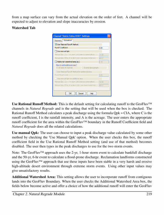
from a map surface can vary from the actual elevation on the order of feet. A channel will be
expected to adjust to elevation and slope inaccuracies by erosion.
Watershed Tab
Use Rational Runoff Method: This is the default setting for calculating runoff to the GeoFluv™
channels in Natural Regrade and is the setting that will be used when the box is checked. The
Rational Runoff Method calculates a peak discharge using the formula Qpk = CIA, where C is the
runoff coefficient, I is the rainfall intensity, and A is the acreage. The user enters the appropriate
runoff coefficient for the area within the GeoFluv™ boundary in the Runoff Coefficient field and
Natural Regrade does all the related calculations.
Use manual Qpk: The user can choose to input a peak discharge value calculated by some other
method by checking the 'Use Manual Qpk' option. When the user checks this box, the runoff
coefficient field in the Use Rational Runoff Method setting (and use of that method) becomes
disabled. The user then types in the peak discharges to use for the two storm events.
Note: The GeoFluv™ approach uses the 2-yr, 1-hour storm event to calculate bankfull discharge
and the 50-yr, 6-hr event to calculate a flood-prone discharge. Reclamation landforms constructed
using the GeoFluv™ approach that use these inputs have been stable in a very harsh and erosive
high-altitude desert environment through extreme storm events. Using other input values may
give unsatisfactory results.
Additional Watershed Area: This setting allows the user to incorporate runoff from contiguous
lands into the GeoFluv Boundary. When the user checks the Additional Watershed Area box, the
fields below become active and offer a choice of how the additional runoff will enter the GeoFluv
Chapter 2. Natural Regrade Module 219

Boundary. If the head of the GeoFluv™ channel is downstream of the Additional Watershed
Area, as when joining to an upstream channel reach, the user should select the ''At head of chan-
nel'' option. The GeoFluv™ channel's headwater dimensions will then be sized to accommodate
the runoff from the area above the channel headwaters within the GeoFluv Boundary and the Ad-
ditional Watershed Area upstream of that. If the Additional Watershed Area is subparallel to the
GeoFluv™ channel, checking ''Evenly along length'' will introduce the runoff from the Additional
Watershed Area gradually along the GeoFluv™ channel reach and the channel dimensions will
increase proportionately along the reach. The remainder of the settings are as described above in
''Use Rational Method'' and ''Use manual Qpk.''
Data for Current Channel
Function
These are the data that GeoFluv™ uses to calculate the drainage density for the subwatershed
containing the channel in the Current Channel field above, and a display window that informs the
user if discharge from additional area outside the GeoFluv Boundary is entering the subwatershed.
These are not input fields, but real-time displays of the values being used in the GeoFluv™ design
for the Current Channel. GeoFluv™ calculates these values from the subwatershed boundary it
has built and the drainage pattern that the user sketched, and user-input additional area by the
Channels tab's ''Advanced . . .'' button.
Valley Length (ft.) This value is the straight-line length of the valley (in feet in U.S. units), not
the sinuous length of the channel.
Reach Area (ac.) This value is the area (in acres in U.S. units) draining water to that channel or
channel reach.
Add'l Area (ac.) This field displays any additional area outside the GeoFluv™ boundary that is
draining into the GeoFluv™ Current Channel. This could be contiguous undisturbed land or land
that has already been reclaimed. The Channels tab's ''Advanced . . .'' button allows the user to
add additional area.
Drainage Density (ft/ac) This value is the ratio of Valley Length to Reach Area in U.S. units of
feet per acre, a convenient unit for this parameter in landform design work.
If the drainage density is within the variance that the user specified in the Design Natural Regrade
dockable dialog box's Settings button, Natural Regrade Global Settings, ''Target drainage density
variance (%)'', then the value will be highlighted in green; if the value is outside the user-specified
variance it will be highlighted in red. A red warning can mean that the drainage density is too high
or too low. If too high, the channel can be shortened or the Current Channel's subwatershed area
Chapter 2. Natural Regrade Module 220

increased. If the value is too low, the Current Channel can be lengthened, or a tributary channel
can be drawn in the Current Channel subwatershed and then added using the Channels tab's Add
button, or the subwatershed area can be decreased.
If the GeoFluv Boundary polyline or the valley bottom polylines are modified in the drawing,
clicking on the Reread Valley Bottoms button will cause the above data to be updated.
Profile
Function
This button activates a popup view window, Profile Viewer, which allows the user to see the
Current Channel's longitudinal profile graphically. Moving the viewer cursor along the profile
allows the user to obtain the station, elevation, and slope at any point indicated by crosshairs
along the profile.
Vertical Exaggeration This toggle button setting allows the user to select profile views at fit, 1x,
2x, 5x, and 10x vertical exaggeration.
Drag Action This toggle button setting allows the user to select either zoom or pan drag action.
Then the user selects the Zoom button, holding down the left-click button on the mouse as the
mouse is moved will zoom in and out on the profile display. Similarly, when the user selects the
Pan button, holding down the left-click button on the mouse allows the user to pan the profile in
Chapter 2. Natural Regrade Module 221

the display. Whether in Zoom mode or Pan mode, the middle mouse button can be held down to
pan the profile in the display. Thus, if the user has a middle mouse button, staying in the Zoom
mode and using the middle mouse button to pan is most efficient.
Grid Ticks Only This toggle button setting allows the user to select either the default x and y
grid lines across the profile, or tick marks only on the axes.
Report
Function
The Report button is used for detailed inspection of the GeoFluv™ Current Channel's design
characteristics.
The report is for the channel as it would be incorporated into the design after using the Draw
Design Surface button on the Output tab. Note that the channels with slopes >-0.04 do not have
the meandering channel geometry relationships that lower slope channels do. Their different
characteristics are designed differently in the GeoFluv™ approach and because of this radius of
curvature, meander length, meander belt width, and meander width ratio are not listed.
The user left-clicks on the Report button and the ''Channel 'xxxx' Report Options'' dialog box
opens. The user can type in the desired station interval for the report in the ''Station Interval:''
window. The user then left-clicks on the OK button and the report for that channel is generated
according to the user-specified stationing.
Chapter 2. Natural Regrade Module 222

The report gives summary design information for the Current Channel and lists channel-reach
detailed information at the user-specified station intervals. The stationing increases in the down-
stream direction with station 00 being the channel head.
Output Tab
Function
The Output Tab allows the user to preview the channels and ridgelines that will be contoured to
reveal the draft GeoFluv™ design landform, to draw and contour the surface, to save the design,
to verify the average drainage density within the GeoFluv Boundary, to compare the cut and fill
volumes needed to create the design and to verify that the cut and fill volumes balance within a
user-specified limit, and to create and view a summary report of the channel settings and design
dimensions.
Chapter 2. Natural Regrade Module 223

Preview
Function
The Preview button displays the channel and main ridgelines from which GeoFluv™ will base its
draft landform design.
Chapter 2. Natural Regrade Module 224

Command Prompt:
The command reads, ''Preview. Use View menu commands to change views. Press Enter to
continue.'' when the Preview button is left-clicked.
Left-clicking on the Preview button draws the main GeoFluv™channel and ridge design lines on
the drawing. The A and A+ channel reaches (>-0.04 slope) are displayed as zig-zag lines. The
valley bottom channel reaches (<-0.04 slope) are displayed as sinuous curved lines. The main
ridgelines are shown between the tributary channels and are sub-parallel to the channels.
Data for GeoFluv Work Area
Function
These are the data that GeoFluv™ uses to calculate the drainage density for the entire area within
the GeoFluv Boundary. These are not input fields, but real-time displays of the values being
used in the GeoFluv™ design for overall project area within the GeoFluv Boundary. GeoFluvTM
calculates these values from the GeoFluv Boundary that the user has drawn and the drainage
pattern that the user sketched.
Valleys (ft.) This value is the combined straight-line length of all the valleys (in feet in U.S. units),
not the sinuous length of the channel, that the user has sketched within the GeoFluv Boundary.
Area (ac.) This value is the area (in acres in U.S. units) within the GeoFluv Boundary.
Chapter 2. Natural Regrade Module 225

Drainage Density (ft/ac) This value is the ratio of Valley Length to Reach Area in U.S. units of
feet per acre, a convenient unit for this parameter in landform design work.
If the drainage density is within the variance that the user specified in the Design Natural Regrade
dockable dialog box's Settings button, Natural Regrade Global Settings, ''Target drainage density
variance (%)'', then the value will be highlighted in green; if the value is outside the user-specified
variance it will be highlighted in red. A red warning can mean that the drainage density is too
high or too low. If too high, channels can be deleted or shortened, or the area within the GeoFluv
Boundary can be increased. If the value is too low, valleys can lengthened, or a tributary channel
can be drawn within the GeoFluv Boundary and then added using the Channels tab's Add button,
or the area within the GeoFluv Boundary can be decreased.
Draw Design Surface
Function
Draw Design Surface integrates all of the GeoFluv™ landform design data that the user has input
and outputs it to the drawing.
Left-clicking on the Draw Design Surface button causes the Draw Design Surface dialog box to
appear. This dialog box allows the user to choose the layer name to which Natural Regrade will
save the channel and ridge polylines, the triangle skirt layer, and the Sub-Watersheds. Toggles in
the dialog box also allow the user to specify:
• If the triangle mesh outside the GeoFluv™ boundary will be drawn.
• If the 2D outlines of subwatersheds will be drawn.
• If intersecting built tributary channels are trimmed at the point of intersection or if they
continue all the way to the confluence.
• If existing entities in these layers are erased.
Chapter 2. Natural Regrade Module 226
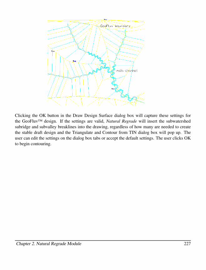
Clicking the OK button in the Draw Design Surface dialog box will capture these settings for
the GeoFluv™ design. If the settings are valid, Natural Regrade will insert the subwatershed
subridge and subvalley breaklines into the drawing, regardless of how many are needed to create
the stable draft design and the Triangulate and Contour from TIN dialog box will pop up. The
user can edit the settings on the dialog box tabs or accept the default settings. The user clicks OK
to begin contouring.
Chapter 2. Natural Regrade Module 227

Natural Regrade will draw the draft GeoFluv™ landform contours on the drawing and a pop-up
Carlson Edit dialog box will appear that lists any instances of 'crossing barrier lines', if the trian-
gulate and contour settings were appropriate. The user can use this edit box to review the drawing
for possible errors; typically the crossing barrier lines reported in this edit box are intersections of
channel and valley lines. (See also the Draw GeoFluv Contours command for more detail about
this feature.)
If the 'maximum triangle mesh line length' setting in the Triangulate tab of the Contour selection
in the Carlson DTM Triangulate and Contour menu is set to a value less than the required triangle
mesh line length for portions of the design, the command line will read ''Ignored 'xxx' triangulation
lines that exceeded maximum tmesh line length'' and only those portions of the design, if any, that
did not exceed the maximum tmesh line length will be contoured. If this occurs, the user can
reset the maximum triangle mesh setting in the DTM menu to be greater than the 'xxx' distance
reported in the command line and then repeat the Draw Design Surface command sequence as
described above. GeoFluv™ will then contour the entire drawing as described above. (See also
the Draw GeoFluv Contours command for more detail about this feature.)
The subridgelines and the valleys between them extend from the main ridgelines to the channels.
The slopes have default settings that create concave slopes, rather than constant gradient or convex
slopes that are subject to rill and gully formation.
Chapter 2. Natural Regrade Module 228

Save Design Surface
Function
The Save Design Surface button provides a quick means to save the triangulation mesh file of
the GeoFluv™ draft design surface. The draft design surface is virtual and is not necessarily
represented in the drawing at the moment. The draft design surface is created using the inputs
of the 2D valley bottom polylines, the GeoFluv Boundary, the Pre-Disturbed Surface, and the
various settings of the current GeoFluv project. The draft design surface is the same one that
would be created by the Draw Design Surface button.
Any modifications to ridge or subridge or channel polylines in the drawing using tools such as
Edit Longitudinal Profile are not a part of the draft design surface. To create a triangulation mesh
file of the design surface in the drawing, use the Draw GeoFluv Contours command in the Natural
Regrade dropdown menu and select the Write Triangulation File option on the Triangulate tab.
The user left-clicks on the Save Design Surface button and the Save Design Surface - (.FLT; .TIN)
dialog box appears on the screen. The user is offered three options to name and save the surface
file. The user can type in the name of a new or existing file in the File Name window, or left-click
on the Browse button to the right of the window to get a list of surface files related to the project.
If the user wants to save surface file as an existing file (overwrite the file), they can highlight the
file name in the Recently Used Files: window at the bottom of the dialog box or in the ''Files in
that folder'' window at the right of the dialog box. The user then left-clicks on the Open button at
the bottom of the dialog box to save the file with the selected name.
Update Cut/Fill
Function
The user can compare the current GeoFluv™ design surface with either the Pre-Disturbed Surface
or the Disturbed Surface that is toggled on in the Output tab. This feature provides a convenient
means for the user to document that editing has achieved a material balance for the GeoFluv™
design.
If the user has toggled Pre-Disturbed Surface in the Output tab's Surface for Cut / Fill option, left-
clicking the Update Cut / Fill button will cause Natural Regrade to compare the GeoFluv™ design
surface to the Pre-Disturbed surface and calculate the volumes of cut and fill material required to
construct the GeoFluv™ design from the Pre-Disturbed Surface. The results of the calculation
are displayed (in English units) as cubic yards of cut, cubic yards of fill, and the percent variance
of cut to fill.
Chapter 2. Natural Regrade Module 229

If the user has toggled Disturbed Surface in the Output tab's Surface for Cut / Fill option, left-
clicking the Update Cut / Fill button will cause Natural Regrade to compare the GeoFluv™ design
surface to the user-selected Disturbed surface and calculate the volumes of cut and fill material
required to construct the GeoFluv™ design from the Disturbed Surface. The results of the cal-
culation are displayed (in English units) as cubic yards of cut, cubic yards of fill, and the percent
variance of cut to fill.
If the cut and fill variance percentage is within the range that the user specified in the Settings,
Natural Regrade Global Settings dialog box, then the Cut / Fill percent variance will be high-
lighted in green to quickly inform the user that they have achieved a desired material balance. If
the cut and fill variance percentage is outside the user-specified range, then the Cut / Fill percent
variance will be highlighted in red to alert the user that they have not achieved a desired material
balance.
Some ways to quickly alter the cut / fill balance in the draft GeoFluvTM design include raising or
lower ridge longitudinal profiles using the editors in Natural Regrade's dropdown menu, changing
the upstream slope percent of channels in the Channels tab, and moving the channel transition
point from >-0.04 reach to <-0.04 reach using the Channels tab's Advanced button.
Summary Report
Function
The Summary Report button provides the user with a quick summary report of the input param-
eters and resulting dimensions and material volumes that Natural Regradeused to design each
GeoFluv™ channel within the project's GeoFluv Boundary.
The user left-clicks on the Summary Report button and the GeoFluv Summary Report dialog box
appears on the screen. The dialog box gives the user the options of creating a custom report
by checking the ''Use report formatter'' box (toggle on) and presenting characteristics of Rosgen
channel types by checking the ''Show Rosgen example channels'' box (toggle on; this is the default
setting).
Chapter 2. Natural Regrade Module 230

This information can be useful to compare the channels' morphology with other natural channel
types when editing the draft GeoFluv™ design to verify that changes to the channel do not exceed
the range established for that stable channel type. The summary report information can also be
useful for estimating if the user may want to increase channel roughness, install additional bank
protection or channel weirs to augment step-pool sequences, etc. Fields that contain information
that is not used in the GeoFluv™ approach for designing A and Aa+ channels (>0.04 slope) are
marked n/a. Many of the channel characteristics occur within a range at any particular reach in
stable natural channels, rather than as a specific value. The dimensions also change in the up-and
downstream directions as a function of discharge. The Summary Report presents the range of
these values that are applicable to the entire length of each channel. The user can report channel
reach-specific information by using the Channels tab's Report button.
DWG Tab
Draw GeoFluv Contours
Function
This command gives the user single-click access to the ''Triangulate and Contour from TIN'' dialog
box via the Natural Regrade drop-down menu.
After the user has used the Design GeoFluv Regrade dockable dialog box/Output tab's Draw
Design Surface button to create the GeoFluv™ design in the drawing, the user can left-click on
Chapter 2. Natural Regrade Module 231

the Draw GeoFluv Contours command and produce the Triangulate and Contour from TIN dialog
box to contour revisions to the polylines in the layers that the GeoFluv™ design was drawn to.
When the contours have been drawn, the Error Log: C:\ Scad2005\User—Trierror.xml dialog
box will appear. The user can review this error log, or close the box and proceed with the contour-
ing if precise detail is not yet required at this design stage. This Error Log reports any potential
errors that Carlson has detected when contouring the drawing.
Chapter 2. Natural Regrade Module 232

For example, if the report has a Crossing Breaklines (two polylines with different elevations) field,
the user can left-click on that field and a list of the detected crossing breaklines will appear. The
user can then left-click on each detected crossing breakline and its x and y coordinates will be
displayed at the bottom of the dialog box. The user may choose to report or draw all the detected
potential problems using the Report All and Draw All buttons, or may highlight to select a single
potential problem. If the user selects a single problem, the buttons change to Report One and
Draw One.
The user can left-click on the Zoom button to inspect the suspected problem; this will zoom to
the relevant area of the drawing and place an arrow that points to the suspected problem on the
drawing. Left clicking on the Zoom In button will allow closer inspection of the area of concern,
and the Zoom Out button will return the user to the previous view.
For example, if only one entity was selected as a problem of concern, the ''Report . . '' button
will indicate Report One and left-clicking on the Report One button brings up the Carlson Edit:
c:\scad2005\USER\scadrprt.tmp dialong box that displays a Crossing Breaklines Report with
the x and y coordinates of the problem, and the elevation difference between the crossing break-
lines. Left clicking on the Draw One button draws the selected potential problem breakline on
the drawing and brings up an AutoCAD dialog box that tells the user that one feature has been
processed.
When the user closes the Error Log dialog box by left-clicking on the X in the upper right corner
or on the Done button, the Error Log dialog box disappears and the contoured GeoFluv™ design
remains on the screen. The user can then choose to edit the drawing using tools in the Natural
Chapter 2. Natural Regrade Module 233

Regrade menu, or any other Carlson menu tools, or can reopen the Design GeoFluv Regrade
dockable dialog box to edit any of the GeoFluv™ settings there.
Pulldown Menu Location: Natural Regrade
Keyboard Command: gfContour
Prerequisite: Design geofluv
File Name: \lsp\geofluv.arx
3D GeoFluv Contour Viewer
Function
This Natural Regrade menu gives the user single-click access to the 3D GeoFluv Contour Viewer
that displays, in 3D, the surface created from the contours of a GeoFluv™ design. Viewing
the contours is more representative of how the landform will look after grading than the surface
produced by the 3D GeoFluv Surface Viewer. The 3D GeoFluv Surface Viewer shows you the
surface based on the GeoFluv™ design, before using Triangulate and Contour. This resulting
surface tends to be angular and faceted, and it is also the surface used for volume calculations.
The 3D GeoFluv Contour Viewer shows you the surface based on the GeoFluv™ design after
using Triangulate and Contour, and therefore has more and smaller triangles, lending a smoother
appearance to the 3D image.
Note that these commands use linework from particular layers in the drawing. This means that
any editing the user makes to the linework in these layers will be reflected in the resulting 3D
image.
The prerequisite to using the 3D GeoFluv Contour Viewer is that the contours must already ex-
ist. To create contours, the user can select the Triangulate and Contour option after clicking on
the Draw Design Surface button on the Output tab of the Design GeoFluv Regrade command.
Alternatively, the user can use the Draw GeoFluv Contours command on the Natural Regrade
drop-down menu, which will create the contours based on the GeoFluv™ design that exists in
particular layers in the drawing.
Clicking on the 3D GeoFluv Contour Viewer command first shows a dialog box asking the user
to verify the layers in the drawing that the contours are in. There is also an option for saving the
surface created from the contours into a TIN file, which can then be used with other tools in other
Carlson Civil / Survey modules. Clicking on the OK button causes the contours in the selected
layers to be ''triangulated'' into a solid surface, or TIN, and then opens the Carlson Software 3D
Viewer with the GeoFluv™ design surface displayed.
Chapter 2. Natural Regrade Module 234

The user has many options for viewing the image available in the View Control tab dialog box
on the right side of the 3D Viewer screen. The 3D project view can be rotated on the x, y, and
z axes using the sliding Rotation Axis controls to the right of the view. By left-clicking and
dragging the slider control below the image, the user can clip off forward portions of the view.
The viewer has the ability to add vertical exaggeration to aid inspection of lower-relief areas by
left-clicking on the arrow to the right of the ''Vert. scale'' edit box and selecting a factor from the
dropdown menu. The viewer can also change the position of the sun on the project to evaluate
sunny and shady areas throughout the day, a very useful tool for identifying optimal areas for
different plantings. The user can either left-click on the 'sun' (yellow box in the blue circle)
and drag is across the 'sky' from the west (the blue circle is the sky) or move the slider buttons
surrounding the blue circle. The 3D viewer has the ability to color the view by elevation layers
by a toggle setting at the top of the dialog box. These views are helpful for construction to help
workers visualize how the final project surface can be built in a series of lifts, for example by
using GPS-guided truck dumping.
The toggle buttons on the dialog box below the blue and yellow 'sun and sky' indicator control:
Pan The user holds down the left-click button and moves the mouse across the drawing to pan the
drawing in the 3D Viewer.
Rotation The 3D project view can be rotated on the x, y, and z axes by left-clicking the rotation
toggle button and then holding down the left-click button while moving the mouse on the drawing.
Dynamic Zoom The user can zoom in and out of the 3D view by holding down the left-click
button and moving the mouse up and down on the drawing.
Chapter 2. Natural Regrade Module 235

Shading The user can toggle to fill with shading (color) between the TIN file's triangular edges
to give the drawing a solid surface appearance.
Average Elevation The user can toggle to have an arrow appear on the drawing surface that
indicates the average elevation at the point at which the arrow points.
Reset to Plan The user can left-click on this button to cancel all rotation settings and return to
plan view.
The Carlson Software 3D Viewer's Advanced tab has options to block model objects, shade the
view, export the view image, and save the view that are fully described in the General Com-
mands/View Commands documentation.
The user can exit the 3D Viewer by left-clicking on the X at the upper right or the door at the
bottom of the dialog box.
Pulldown Menu Location: Natural Regrade
Keyboard Command: gfViewC
Prerequisite: Design geofluv
File Name: \lsp\geofluv.arx
3D GeoFluv Surface Viewer
Function
This Natural Regrade command gives the user single-click access to a 3D GeoFluv™ surface
viewer that is based on the GeoFluvTM design. The 3D GeoFluv Surface Viewer displays, in 3D,
the surface created from the linework that was drawn by the Design GeoFluv Regrade command.
This resulting surface is the same one that is used for volume calculations. Alternatively, the 3D
GeoFluv Contour Viewer displays, in 3D, the surface created from the contours of a GeoFluvTM
design which has more and smaller triangles lending a smoother appearance to the 3D image.
Note that these commands use linework from particular layers in the drawing. This means that
any editing the user makes to the linework in these layers will be reflected in the resulting 3D
image.
The prerequisite to using the 3D GeoFluv Surface Viewer is that the linework for a GeoFluvTM
design must already exist in the drawing. To create the GeoFluvTM design in the drawing, the user
can click on the Draw Design Surface button on the Output tab of the Design GeoFluv Regrade
command.
Clicking on the 3D GeoFluv Surface Viewer command causes the 3D Surface Viewer dialog box
to appear on the screen.
Chapter 2. Natural Regrade Module 236

The user has many options for viewing the image available in the View Control tab dialog box
on the right side of the 3D Viewer screen. The 3D project view can be rotated on the x, y, and
z axes using the sliding Rotation Axis controls to the right of the view. By left-clicking and
dragging the slider control below the image, the user can clip off forward portions of the view.
The viewer has the ability to add vertical exaggeration to aid inspection of lower-relief areas by
left-clicking on the arrow to the right of the ''Vert. scale'' edit box and selecting a factor from the
dropdown menu. The viewer can also change the position of the sun on the project to evaluate
sunny and shady areas throughout the day, a very useful tool for identifying optimal areas for
different plantings. The user can either left-click on the 'sun' (yellow box in the blue circle)
and drag is across the 'sky' from the west (the blue circle is the sky) or move the slider buttons
surrounding the blue circle. The 3D viewer has the ability to color the view by elevation layers
by a toggle setting at the top of the dialog box. These views are helpful for construction to help
workers visualize how the final project surface can be built in a series of lifts, for example by
using GPS-guided truck dumping.
The toggle buttons on the dialog box below the blue and yellow 'sun and sky' indicator control:
Pan The user holds down the left-click button and moves the mouse across the drawing to pan the
drawing in the 3D Viewer.
Rotation The 3D project view can be rotated on the x, y, and z axes by left-clicking the rotation
toggle button and then holding down the left-click button while moving the mouse on the drawing.
Chapter 2. Natural Regrade Module 237

Dynamic Zoom The user can zoom in and out of the 3D view by holding down the left-click
button and moving the mouse up and down on the drawing.
Shading The user can toggle to fill with shading (color) between the TIN file's triangular edges
to give the drawing a solid surface appearance.
Average Elevation The user can toggle to have an arrow appear on the drawing surface that
indicates the average elevation at the point at which the arrow points.
Reset to Plan The user can left-click on this button to cancel all rotation settings and return to
plan view.
The Carlson Software 3D Viewer's Advanced tab has options to block model objects, shade the
view, export the view image, and save the view that are fully described in the General Com-
mands/View Commands documentation.
The user can exit the 3D Viewer by left-clicking on the X at the upper right or the door at the
bottom of the dialog box.
Pulldown Menu Location: Natural Regrade
Keyboard Command: gfView3D
Prerequisite: Design geofluv
File Name: \lsp\geofluv.arx
Calculate GeoFluv Volume
Function
This Natural Regrade drop-down menu command is used to calculate the cut and fill volume
difference between the GeoFluvTM design surface in the drawing and another surface, the Com-
parison Surface. The Comparison Surface is specified on the Output tab. Possible sources for the
Comparison Surface may be pre-disturbed, such as the natural landsurface or an earlier reclama-
tion design, or may be disturbed, such as a mine pit or construction site.
If the valley bottom or GeoFluv Boundary polylines have been moved, or any setting in the
GeoFluv project has been changed that can affect volumes, then the design surface in the drawing
will be out-of-date. The ''Draw Design Surface'' button must be used to create a new surface in
the drawing to reflect the changes.
When the user clicks on the command, a dialog box appears with the cut and fill required to
transform the first surface into the current design surface (layers GF Channels and GF Ridges).
The first surface is the Comparison Surface. The cut and fill are calculated wherever the two
Chapter 2. Natural Regrade Module 238

surfaces overlap unless an inclusion polyline is given in which case the cut and fill are calculated
within the inclusion polyline.
The results are displayed in cubic yards in the English system of units and cubic meters in the
metric system.
Pulldown Menu Location: Natural Regrade
Keyboard Command: gfVolume
Prerequisite: Design geofluv
File Name: \lsp\geofluv.arx
Cut/Fill Centroids
Function
This Natural Regrade dropdown menu command is designed to show the amounts and locations of
cut and fill that are required to transform the Comparison Surface (typically the disturbed surface)
into the design surface. The Comparison Surface is specified in the current GeoFluv™ project on
the Output tab. The design surface for this command is the result of combining the GeoFluv™
design in the layers in the drawing within the GeoFluv Boundary plus the Surface for Elevations
(specified on the Setup tab) outside the GeoFluv Boundary.
After comparing these two surfaces, this command identifies the centers of earth-material volumes
that need to be moved and the centers of voids that need to be filled to create the GeoFluv™
design. The command includes the option to identify optimal straight-line material movement
paths.
Note that this command uses linework from particular layers in the drawing. This means that any
editing the user makes to the linework in these layers will be reflected in the results.
The prerequisites for using the Cut Fill Centroids command is that the linework for a GeoFluvTM
design must already exist in the drawing and the Comparison Surface must be set. To create
the GeoFluvTM design in the drawing, the user can click on the Draw Design Surface button on
the Output tab of the Design GeoFluv Regrade command. The Comparison Surface file can be
entered by clicking on the Comparison Surface button on the Design GeoFluv Regrade Output
tab.
Clicking on the Cut Fill Centroid command causes the Cut & Fill Centroid Locator dialog box to
appear, if the prerequisites have been met. The Cut & Fill Centroid Locator dialog box gives the
user several options.
Chapter 2. Natural Regrade Module 239

Minimum Region Volume allows the user to type a minimum cut / fill centroid region volume
for the calculations into an edit box.
Generate Labels is a toggle setting that allows the user to have the centroid region number, cut
or fill, and volume value labeled on the drawing next to a crosshair that indicates the centroid
coordinates.
Text Size Scaler: Allows the user to type a scale factor into an edit box to enlarge or reduce the
size of label text. This command is inactive when Generate Labels is toggled off.
Layer: Allows the user to specify the layer on which the labels will be drawn by either typing
them into an edit box or by left-clicking on the Select button which produces a dropdown list of
existing layers from which to choose. The user can highlight a layer name on the list and click
OK at the bottom of the dropdown menu to select a layer.
Generate Boundaries is a toggle setting that allows the user to specify if Natural Regrade shall
create cut / fill boundaries and, if so, to what layer the boundaries should be saved. If toggled
off, the edit window is inactive. When toggled on, the user may accept the default boundary layer
name, type a different boundary layer name into the edit box, or left-click on the Select button to
choose from the list of layers.
Hatch Regions is a toggle setting that allows the user to have the centroid regions covered with
hatching to make it easier to discriminate from other parts of the drawing.
Chapter 2. Natural Regrade Module 240

Hatch Scale: Allows the user to type a scale factor into an edit box to enlarge or reduce the size
of hatching. If the user specifies a scaler that causes the hatch spacing to be too dense or the dash
size too small, this error will be reported on the Command Line. [Tip: Before drawing a different
scale, erase the previous iteration using Edit/Erase/Erase by layer.] This command is inactive
when Hatch Regions is toggled off.
Layer: Allows the user to specify the layer on which the hatching will be drawn by either typing
the layer name into an edit box or by left-clicking on the Select button which produces a dropdown
list of existing layers from which to choose. The user can highlight a layer name on the list and
click OK at the bottom of the dropdown menu to select a layer.
Hatch Styles: Allows the user to specify hatch styles to differentiate among Fill, Zero elevations
between Fill and Cut, and Cut material by either typing them into an edit box or by left-clicking
on the Select button which produces a dropdown list of existing layers from which to choose. The
user can highlight a layer name on the list and click OK at the bottom of the dropdown menu to
select a layer.
Report Optimized Earth Movement is a toggle setting that allows the user to specify if Natural
Regrade shall not only calculate and identify the cut and fill centroids, but also determine the
shortest straight-line haul distances to distribute the material from cut to fill regions.
When the user is satisfied with the settings on the Cut & Fill Centroid Locator dialog box,
Chapter 2. Natural Regrade Module 241
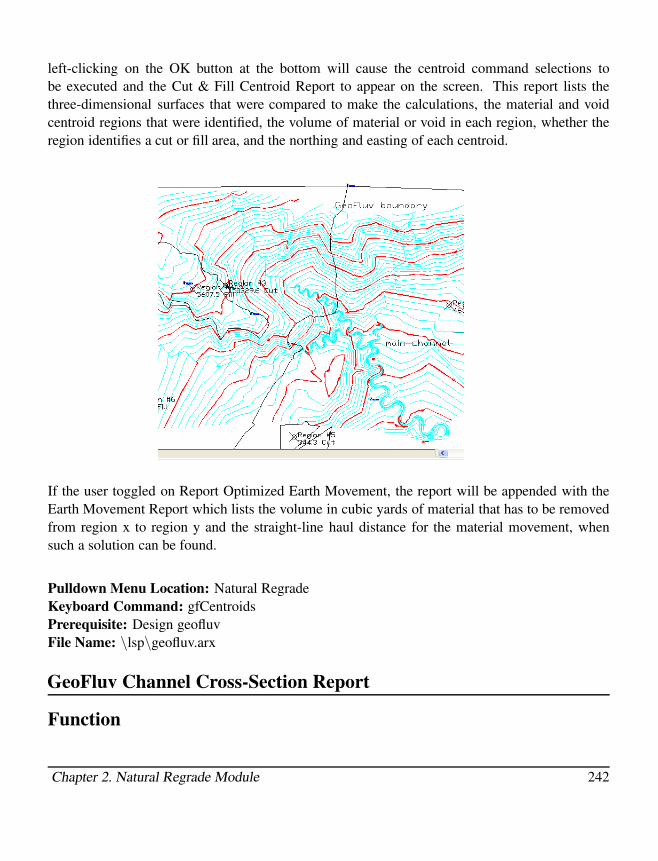
left-clicking on the OK button at the bottom will cause the centroid command selections to
be executed and the Cut & Fill Centroid Report to appear on the screen. This report lists the
three-dimensional surfaces that were compared to make the calculations, the material and void
centroid regions that were identified, the volume of material or void in each region, whether the
region identifies a cut or fill area, and the northing and easting of each centroid.
If the user toggled on Report Optimized Earth Movement, the report will be appended with the
Earth Movement Report which lists the volume in cubic yards of material that has to be removed
from region x to region y and the straight-line haul distance for the material movement, when
such a solution can be found.
Pulldown Menu Location: Natural Regrade
Keyboard Command: gfCentroids
Prerequisite: Design geofluv
File Name: \lsp\geofluv.arx
GeoFluv Channel Cross-Section Report
Function
Chapter 2. Natural Regrade Module 242

TheNatural Regrade dropdown menu's GeoFluv Channel Cross-Section Report gives the user
single click access to the detailed-by-station GeoFluv™ channel cross section Report that the user
can create using the Channel's tab in the Design GeoFluv Regrade dockable dialog box when not
actively working in the design. A user can select any GeoFluv™-designed channel in a drawing
without any other files and generate this report.
Refer to the Channels tab's Report button description for details of the report.
Command prompt:
Select any channel polyline created by GeoFluv. Select objects:
Pulldown Menu Location: Natural Regrade
Keyboard Command: gfReport
Prerequisite: Design geofluv
File Name: \lsp\geofluv.arx
GeoFluv Channel Inspector
Function
This command allows the user to obtain detailed design information from the Natural Regrade
drawing by passing the cursor over the point of interest (on a polyline in the drawing).
Chapter 2. Natural Regrade Module 243

When the user left-clicks once on the GeoFluv Channel Inspector command in the Natural Re-
grade dropdown menu, a check mark appears to the left of the command signaling the user that
the command is toggled on. Then when the user passes the cursor over any polyline in the draw-
ing, detailed GeoFluv design information for that point on the polyline appears on the screen
next to the cursor. The command remains active until the user left-clicks on the command in the
dropdown menu to toggle it off.
The GeoFluv Channel Inspector works on ridge, valley, and contour polylines also, but obviously
does not present channel design information for those polylines. This convenient and powerful
feature allows the user to inspect designs without having to refer back and forth from a database
to the drawing, but instead read directly from the drawing. Note that the information displayed is
not an average for the entire line, but is specific to location on the line and can vary even in very
small distances.
There are some limitations to be aware of. First, to inspect the zig-zag A-channel, the GeoFluv
project that was used to create that channel must currently be open in the Design Geofluv Regrade
tool. Secondly, using almost any command, including Edit Longitudinal Profile and Auto Longi-
tudinal Profile, to modify a channel polyline causes the extended entity data to be removed which
prevents the GeoFluv Channel Inspector from having certain information that it needs.
Pulldown Menu Location: Natural Regrade
Keyboard Command: gfInspect
Prerequisite: Design geofluv
Chapter 2. Natural Regrade Module 244

File Name: \lsp\geofluv.arx
View Longitudinal Profile
Function
This Natural Regrade dropdown menu command allows the user to view the longitudinal profile
of any polyline in the GeoFluv™ design and obtain the elevation and slope at any point along the
profile.
Command prompt:
Select objects
The user places the cursor over the polyline that they want to inspect and left-clicks. The profile
viewer appears on the screen. The user can move the cursor along the profile and the station,
elevation, and slope information are displayed along the bottom of the dialog box at the posi-
tion indicated by the cursor. Simultaneously, an arrow moves along the channel in the drawing
pointing to the location along the longitudinal profile that the cursor is covering on the profile
viewer.
Radio buttons for Vertical Exaggeration settings aid the user in evaluating low relief profiles.
Radio buttons also allow the user to toggle back and forth between Zoom and Pan drag action
for the mouse. When set to Zoom, holding the mouse left-click button down while moving the
Chapter 2. Natural Regrade Module 245

mouse up and down will cause the viewer to zoom in and out on the longitudinal profile. When
set to Pan, holding the mouse left-click button down while moving the mouse across the viewer
will allow the user to pan around the longitudinal profile. Whether in Zoom mode or Pan mode,
the middle mouse button can be held down to pan the profile in the display. Thus, if the user has
a middle mouse button, staying in the Zoom mode and using the middle mouse button to pan is
most efficient.
The Grid Ticks Only toggle allows the user to see a grid on the profile display or to see only tick
marks on the axes.
Pulldown Menu Location: Natural Regrade
Keyboard Command: gfViewPro
Prerequisite: Design geofluv
File Name: \lsp\geofluv.arx
Edit Longitudinal Profile
Function
The Natural Regrade dropdown menu's Edit Longitudinal Profile command gives the user quick
access to a powerful longitudinal profile editing tool that can change the entire longitudinal profile
of a 3D polyline or just a portion of the profile.
Examples of tasks that this profile editor is well suited for is creating saddles on a long ridge line
to further dissect topography and creating a 'hump' on the ridge profile where the user might want
to leave excess material.
When the user left-clicks on Edit Longitudinal Profile, the command line directs the user to Select
3D Polyline and the command prompt reads, ''Select objects:.'' The user moves the cursor to the
3D polyline that they wish to edit and left-clicks on the polyline. The ''Edit Longitudinal Profile
– Double Click to Adjust Profile'' pop-up dialog box appears on the screen. The dialog box has a
profile viewer similar to the View Longitudinal Profile command viewer. The user can move the
cursor along the profile and the station, elevation, and slope information are displayed along the
bottom of the dialog box at the position indicated by the cursor. Simultaneously, an arrow moves
along the channel in the drawing locating the point along the longitudinal profile that the cursor
is covering.
Chapter 2. Natural Regrade Module 246

The dialog box gives the user toggle settings for the following options:
Adjust connecting linework, when toggled on (the default setting) by left-clicking on the box,
will cause Natural Regrade to automatically change all connecting linework, e.g., connecting
ridges, to smoothly fit the new longitudinal profile. To update contours to reflect the modified
surface, the Draw GeoFluv Contours command can be used.
Grid Ticks Only toggle allows the user to see a grid on the profile display or to see only tick
marks on the axes.
Radio buttons give the user the following options:
Vertical Exaggeration settings aid the user in evaluating low relief profiles.
Zoom and Pan drag action for the mouse - When set to Zoom, holding the mouse left-click button
down while moving it up and down will cause the viewer to zoom in and out on the longitudinal
profile. When set to Pan, holding the mouse left-click button down while moving it around the
viewer will allow the user to pan around the longitudinal profile. Whether in Zoom mode or Pan
mode, the middle mouse button can be held down to pan the profile in the display. Thus, if the
user has a middle mouse button, staying in the Zoom mode and using the middle mouse button to
pan is most efficient.
A slider button on the Blend 'x'% control allows the user to specify the percentage of the polyline
to which they want to apply the profile change. As the user holds down the mouse left-click button
Chapter 2. Natural Regrade Module 247

on the slider button and moves the slider button left to right, the percentage of the line that will be
affected by the edit is displayed above the slider.
When the user has specified the settings that they want to use for the edit, they move the cursor
above or below the longitudinal profile in the display to the elevation that they want to raise or
lower the profile at that point and double left-click on the mouse. The profile will raise at that
point to the specified elevation and the line will blend from that elevation to the remaining profile
over the distance specified using the ''Blend 'x' %'' slider control. The user can make multiple
adjustments to the longitudinal profile in this fashion until the desired profile is achieved. The
user then left-clicks on the OK button to apply the changes. Left clicking on the Cancel button
will close the dialog box without applying the changes.
Command Prompt:
Select objects:
Pulldown Menu Location: Natural Regrade
Keyboard Command: gfEditPro
Prerequisite: Design geofluv
File Name: \lsp\geofluv.arx
Auto Longitudinal Profile
Function
The Natural Regrade dropdown menu's Auto Longitudinal Profile command gives the user quick
access to a powerful longitudinal profile editing tool that can change the entire longitudinal profile
of a 3D polyline or just a portion of the profile in a smooth curve by specifying starting and ending
slopes.
When the user left-clicks on Auto Longitudinal Profile, the command line directs the user to
Select 3D Polyline and the command prompt reads, ''Select objects:''. The user selects the 3D
polyline that they wish to edit and left-clicks on it. The Auto Longitudinal Profile pop-up dialog
box appears, which gives the user the following options.
Chapter 2. Natural Regrade Module 248

Top Slope can be user-specified by typing a value into the edit box, or the default value, which is
the present value for the selected 3D polyline, can be accepted. When the user exits the edit box,
e.g., with Tab key, an entered slope value is applied to the profile and the user can inspect the
revision on the profile viewer. The user can make multiple adjustments to the longitudinal profile
in this fashion until the desired profile is achieved. This setting will be the slope at the upper end
of the longitudinal profile.
Bottom Slope can be user-specified by typing a value into the edit box, or the default value, which
is the present value for the selected 3D polyline, can be accepted. When the user exits the edit
box, e.g., with Tab key, an entered slope value is applied to the profile and the user can inspect the
revision on the profile viewer. The user can make multiple adjustments to the longitudinal profile
in this fashion until the desired profile is achieved. This setting will be the slope at the lower end
of the longitudinal profile.
Connect to Ridge allows the user to allow a longitudinal profile, e.g., on a ridgeline, to have an
extended convex profile before beginning its concave longitudinal profile. When toggled off (the
default setting with the ''Convex curve length (ft.)'' edit box inactivated), the GeoFluv™ approach
will design a longitudinal profile between the upper and lower elevations of the 3D polyline by
constructing a vertical curve using the specified bottom and top slope percents. When toggled on,
the ''Convex curve length (ft.)'' edit box is activated and the user can type in a desired distance
value that the upper end of the profile can remain convex before the GeoFluv™ vertical curve is
applied using the specified Top Slope percentage. This feature can be used to place extra material
in a hump, for example on a ridgeline, and still have the face of the material grade in a concave
profile toward the valley bottom.
Chapter 2. Natural Regrade Module 249

When Adjust connecting linework is toggled on (the default setting) by left-clicking on
the box, Natural Regrade will automatically change all connecting linework, e.g., connecting
ridges, to smoothly fit the new longitudinal profile. To update contours to reflect the modified
surface, the Draw GeoFluv Contours command can be used.
The dialog box has a profile viewer similar to the Edit Longitudinal Profile command viewer.
The user can move the cursor along the profile and the station, elevation, and slope informa-
tion are displayed along the bottom of the dialog box at the position indicated by the cursor.
Simultaneously, an arrow moves along the channel in the drawing pointing to the point along the
longitudinal profile that the cursor is covering.
Radio buttons for Vertical Exaggeration settings aid the user in evaluating low relief profiles.
Radio buttons also allow the user to toggle back and forth between Zoom and Pan drag action
for the mouse. When set to Zoom, holding the mouse left-click button down while moving it up
and down will cause the viewer to zoom in and out on the longitudinal profile. When set to Pan,
holding the mouse left-click button down while moving it around the viewer will allow the user
to pan around the longitudinal profile. Whether in Zoom mode or Pan mode, the middle mouse
button can be held down to pan the profile in the display. Thus, if the user has a middle mouse
button, staying in the Zoom mode and using the middle mouse button to pan is most efficient.
Grid Ticks Only toggle allows the user to see a grid on the profile display or to see only tick
marks on the axes.
When the user has specified the settings that they want to use for the edit, they then left-click on
the OK button to apply the changes. The new vertical curve will be applied to the GeoFluv™
design.
Pulldown Menu Location: Natural Regrade
Keyboard Command: gfAutoPro
Prerequisite: Design geofluv
File Name: \lsp\geofluv.arx
Reread Valley Bottoms
Function
This command updates GeoFluv with information about changes to the valley bottom polylines
(or GeoFluv Boundary polyline).
The valley bottom and GeoFluv Boundary 2D polylines are user inputs for fundamental values to
Chapter 2. Natural Regrade Module 250

the GeoFluv program. They are used to directly calculate valley length, subwatershed area, and
drainage density, and affect discharge calculations and channel dimensions. All commands that
need to use these input polylines always check the drawing first and use the current version of
these polylines in the drawing. The primary use of this command is to quickly update the data
displayed on the Setup tab, the Channels tab and the Output tab after a change has been made in
the drawing to either the GeoFluv Boundary polyline or any valley bottom polyline.
Chapter 2. Natural Regrade Module 251

Index
3D GeoFluv Contour Viewer, 234
3D GeoFluv Surface Viewer, 236
3D Polyline Flow Values, 21
Advanced Weir Design, 74–76
Auto Longitudinal Profile, 248
Boundaries, 240
Boundary, 188–190, 201, 208–213, 215,
217, 219–221, 223, 225, 226, 229,
230, 238, 239, 250, 251
C-factor, 25
Calculate C-Factor, 25
Calculate GeoFluv Volume, 238
Calculate Stage-Storage, 86
CAP files, 38, 88
Centerline, 48, 113
Centroids, 239, 242
Channel Add, 213
Channel Delete, 214
Channel Design - Erodible Mannings Equa-
tion, 99
Channel Design - NonErodible Mannings
Equation, 97
Channel Name, 215
Channels Tab, 212
Channel Transition, 215
Check Reference Centerlines and Surface,
157
Check Sewer Network Parameters, 156
Collision Conflicts Check, 157–159
Contours, 83, 228
Crossing Breaklines, 233
Culvert Design, 101, 105
Current Channel, 216, 220, 221, 223
Current Channel Settings, 216
Curve Numbers & Runoff, 23, 27, 30, 31, 65
Custom, 63, 124, 125
Cut/Fill Centroids, 239
Data Entry, 197
Data for Current Channel, 220
Data for GeoFluv Work Area, 225
Data for Main Channel, 210
Define Runoff Layers, 7, 13, 151
Description of Software, 184
Design GeoFluv Regrade, 199, 200, 202,
234, 236, 239, 243
Design Spillway, 70
Detention Pond Sizing, 65
Disturbed Area, 4
Documentation References, 199
Drainage Runoff Library, 140, 141
Draw Design Surface, 226–228, 231, 234,
236, 238, 239
Draw Flow Polylines, 36, 45
Draw Flow Polylines TR20, 36
Draw GeoFluv Contours, 231, 232, 234,
247, 250
Draw Hec-Ras Watermark, 53
Draw Hydrograph, 43, 44
Draw IDF Curve, 172–174
Drawing Setup, 92, 99, 207
Draw Pipe, 105, 106, 167
Draw Profile, 167
Draw Sewer Network-3DFaces, 169
Draw Sewer Network Centerlines, 166
252

Draw Sewer Network Plan View, 166
Draw Sewer Network Profile, 167
Draw Stage-Discharge Graph, 94
Draw Stage-Storage Curve, 87
Draw Watermark, 64
Drop Pipe Spillway Design, 71, 97
DWG Tab, 231
Edit Layout Element, 40
Edit Longitudinal Profile, 246, 250
Edit Sewer Structure, 144, 164, 174
Export To Points, 175
Export To Profiles, 176
Extrapolate, 20
Find And Replace Data Values, 174
Find Sewer Structure, 159
GeoFluv Channel Cross-Section Report,
242, 243
GeoFluv Channel Inspector, 243, 244
Geometric Data, 51, 52, 55, 58
Grid File, 6, 20, 86
HEC-2, 48, 60–64, 77, 126–129, 131, 150,
153
HEC-RAS, 2, 48–60
HEC2 Programs, 60
HYDRA Processing, 141
Hydrograph, 27, 41, 42, 163
Hydrograph Development, 36, 38, 39, 41, 43
Hydrology Module, 1, 2, 74, 77, 86, 107,
126, 130, 145, 156, 160, 174
Import Flow Depth Points, 57, 59, 60
Import Flow Velocity Points, 54, 56, 57
Import Haestad Network, 118
Inlet Library, 125, 126, 129, 130, 149
Input-Edit Stage-Discharge, 92–94
Input-Edit Stage-Storage, 81, 82, 85, 86
Introduction and Overview, 179
Join, 36, 37, 45
Landuse, 3
Lift Station Design, 109
Limitations of, 179, 180
Links with Other Software, 196
Locate Reach, 39, 41
Locate Structures TR20, 38
Manhole, 130
Merge Stage-Discharge Files, 96
Move Sewer Label, 170, 171
Multiple Outlet Design, 79–81
Natural Regrade File, 200
Natural Regrade Global Settings, 201, 202,
204, 211, 220, 226
Natural Regrade Menu, 199, 200
Natural Regrade Module, 178
Network Menu, 113
Orifice Design, 76, 77, 79
Output Tab, 223
Overview, 2
Pavement Manning's N Library, 139
Pavement Manning's N Library, 139, 140
Peak Flow - Graphical Method, 30
Peak Flow - Rational Method (General), 34
Peak Flow - Rational Method (KYDOT), 35
Peak Flow - Tabular Hydrograph Method, 31
Pipe Culvert Design, 100, 101, 106
Pipe Manning's N Library, 138
Pipe Manning's N Library, 137, 138
Pipe Size, 102, 148, 152
Pipe Size Library, 134, 135, 137, 142, 152
Plan View Label Settings, 115
Pond Design, 83
Index 253

Pond Sizing, 30, 31, 34
Pre-disturbed Surface, 211, 212
Prepare HEC-RAS Input File, 48, 50, 54, 55,
58
Prepare HEC2 Input File, 61
Preview, 224, 225
PRO, 49, 109
Problems Addressed by Natural Regrade
with GeoFluv, 179
Profile, 221, 229, 244
Rainfall Frequency and Amount, 21
Rainfall Library, 119, 120, 125, 146, 161
Rational Method, 7, 35, 119, 150, 154, 220
Rectangular Pond Design, 66, 67, 84, 87
Rectangular Weir Design, 73
Remove Sewer Structure, 155
repackaged, vi
Report, 222, 231, 233, 241–243
Report Sewer Network, 160, 162
Report Stage-Discharge, 95
Reread Valley Bottoms, 250
Reverse Polyline, 49
Review Sewer Network Links, 175
Review Sewer Profile Links, 175
Runoff, 4, 15, 19, 22, 25, 31, 32, 34, 35, 98,
140, 141, 151, 187, 216, 219
Run Off Tracking, 19, 21, 28
Save Design Surface, 229
Save Sewer Network File, 118
Section Alignment, 50
Section File, 64
SEDCAD, 2, 6, 45–47, 88
SEDCAD Draw Flow Polylines, 45
SEDCAD Label Structure Layout, 46
SEDCAD Locate Structures, 45
Select GeoFluv Boundary, 207
Select Main Channel, 208, 211
Set Sewer File, 114, 169
Set Surface File, 114, 145
Setup Tab, 207
Sewer, 107–109, 117, 118, 141–143, 147,
156, 160, 161, 166–170, 175–177
Sewer Network, 8, 108, 150, 151, 153, 154,
156–158, 161–163, 167, 169, 170,
174–177
Sewer Network Hydrographs, 162–164
Sewer Network Settings, 113, 147
Sewer Pipe Design: Individual, 106
Sewer Pipe Design: Read Profile, 108
Sewer Pipe Design: Sewer Network Seg-
ment, 107, 108
Sewer Structure, 7, 114, 115, 117, 131, 141,
143, 144, 146, 155, 168
Sewer Structure Library, 130, 131, 134, 149,
169
Single Runoff Hydrograph, 42
Slope Ratio, 84
Software Compatibility, 197
Spillway, 38, 68–73, 90, 94
Spillway Design, 97
Spreadsheet Sewer Editor, 164, 165
Stage-Discharge, 38, 75–81, 92–97, 102,
103
Stage-Storage, 82–85, 87, 91, 92, 96
Stage Storage, 87
Steady Flow Data, 52
Stream Network, 48–50
Structure Layout, 45–47
Structure Menu, 64
Sub-Watersheds By Land Use, 22
Summary, 197
Summary Report, 230, 231
Surface Menu, 2
Surface Model, 20, 52, 54
Symbol Size, 149
Index 254
Tabular Hydrograph Method, 32
Text Size, 240
The Fluvial Geomorphic Solution, 181
Time of Concentration, 21, 23, 31
Time of Concentration (Tc), 27, 29
Transit, 215
Triangulation, 19, 229
Universal Soil Loss, 3, 4
Update Cut/Fill, 229
Valley Pond, 64, 70
Valley Pond Design, 38, 73, 87
View, 68, 106, 107, 109, 117, 166, 234–238,
246
View Longitudinal Profile, 245, 246
Volume, 24, 27, 42, 69, 71, 73, 82, 86, 191,
239, 240
Watershed Above Point, 15
Watershed Analysis, 12, 13, 17–19, 148
Watershed Menu, 6
Watershed Settings (Save and Load), 36
Wild, 199
Index 255