CARDIFF UNIVERSITY School of Physics and … FORMULAE AND PHYSICAL CONSTANTS 1 Contents 1 ELEMENTARY...
41
Transcript of CARDIFF UNIVERSITY School of Physics and … FORMULAE AND PHYSICAL CONSTANTS 1 Contents 1 ELEMENTARY...
CARDIFF UNIVERSITY
School of Physics and Astronomy
MATHEMATICAL FORMULAE
AND PHYSICAL CONSTANTS
1
Contents
1 ELEMENTARY ALGEBRA AND TRIGNOMETRY 5
1.1 Logarithms and exponentials . . . . . . . . . . . . . . . . . . . . . . . 5
1.2 Trigonometric functions . . . . . . . . . . . . . . . . . . . . . . . . . 5
1.3 Compound formulae: sines, cosines and tangents . . . . . . . . . . . . 5
1.4 Double-angle formulae . . . . . . . . . . . . . . . . . . . . . . . . . . 5
1.5 "Tan of half-angle" formulae . . . . . . . . . . . . . . . . . . . . . . . 5
1.6 Triangle sine and cosine formulae . . . . . . . . . . . . . . . . . . . . 6
1.7 Hyperbolic functions . . . . . . . . . . . . . . . . . . . . . . . . . . . 6
1.8 Stirling's approximation . . . . . . . . . . . . . . . . . . . . . . . . . 6
2 SERIES FORMULAE 7
2.1 Sums of progressions to n terms . . . . . . . . . . . . . . . . . . . . 7
2.2 Binomial series . . . . . . . . . . . . . . . . . . . . . . . . . . . . . . 7
2.3 Taylor's Theorem . . . . . . . . . . . . . . . . . . . . . . . . . . . . 7
2.4 Power series in algebra and trigonometry . . . . . . . . . . . . . . . 8
3 DERIVATIVES AND INTEGRALS 9
3.1 Derivatives . . . . . . . . . . . . . . . . . . . . . . . . . . . . . . . . 9
3.2 Partial di�erentiation . . . . . . . . . . . . . . . . . . . . . . . . . . . 9
3.3 Inde�nite integrals . . . . . . . . . . . . . . . . . . . . . . . . . . . . 9
3.4 Inde�nite integrals involving sines, cosines and exponentials . . . . . 10
3.5 Integration by parts . . . . . . . . . . . . . . . . . . . . . . . . . . . 10
3.6 De�nite integrals involving sines and cosines . . . . . . . . . . . . . . 10
3.7 De�nite integrals involving exponentials . . . . . . . . . . . . . . . . 11
3.8 Numerical integration . . . . . . . . . . . . . . . . . . . . . . . . . . 11
3.8.1 Trapezoidal rule . . . . . . . . . . . . . . . . . . . . . . . . . . 12
3.8.2 Simpson rule . . . . . . . . . . . . . . . . . . . . . . . . . . . 12
3.9 Newton-Raphson Method for Finding the Root of an Equation . . . 12
4 COMPLEX NUMBERS 13
4.1 De�nitions etc. . . . . . . . . . . . . . . . . . . . . . . . . . . . . . . 13
4.2 De Moivre's theorem . . . . . . . . . . . . . . . . . . . . . . . . . . . 13
2
4.3 Formulae involving eiθ etc. . . . . . . . . . . . . . . . . . . . . . . . . 13
5 SPECIAL FUNCTIONS 14
5.1 Spherical harmonics . . . . . . . . . . . . . . . . . . . . . . . . . . . . 14
5.2 The gamma function . . . . . . . . . . . . . . . . . . . . . . . . . . . 14
5.3 Bessel functions . . . . . . . . . . . . . . . . . . . . . . . . . . . . . 15
6 DETERMINANTS AND MATRICES 16
6.1 De�nition of a determinant . . . . . . . . . . . . . . . . . . . . . . . . 16
6.2 Consistency of n simultaneous equations with n variables and no con-stants. . . . . . . . . . . . . . . . . . . . . . . . . . . . . . . . . . . . 16
6.3 Solutions of n simultaneous equations with n variables and with con-stants. . . . . . . . . . . . . . . . . . . . . . . . . . . . . . . . . . . . 17
6.4 Matrices: basic equations . . . . . . . . . . . . . . . . . . . . . . . . . 17
6.5 Rules of matrix algebra . . . . . . . . . . . . . . . . . . . . . . . . . . 18
6.6 Trace of a square matrix . . . . . . . . . . . . . . . . . . . . . . . . . 18
6.7 Transpose of matrix . . . . . . . . . . . . . . . . . . . . . . . . . . . . 18
6.8 Inverse of a matrix . . . . . . . . . . . . . . . . . . . . . . . . . . . . 18
6.9 Special matrices . . . . . . . . . . . . . . . . . . . . . . . . . . . . . . 18
6.10 Eigenvalues and eigenvectors of a square matrix . . . . . . . . . . . . 19
6.11 Similarity transform . . . . . . . . . . . . . . . . . . . . . . . . . . . 19
6.12 Diagonalisation of a matrix A with di�erent eigenvalues . . . . . . . . 19
6.13 Representation of a rotation by a matrix R . . . . . . . . . . . . . . . 19
7 VECTORS 20
7.1 De�nition of the scalar (or dot) product of two vectors . . . . . . . . 20
7.2 Properties of the scalar product . . . . . . . . . . . . . . . . . . . . . 20
7.3 De�nition of the vector (or cross) product of two vectors . . . . . . . 20
7.4 Properties of the vector product . . . . . . . . . . . . . . . . . . . . . 20
7.5 Scalar triple product . . . . . . . . . . . . . . . . . . . . . . . . . . . 21
7.6 Vector triple product . . . . . . . . . . . . . . . . . . . . . . . . . . . 21
7.7 The del operator ∇ . . . . . . . . . . . . . . . . . . . . . . . . . . . 21
7.8 The gradient of a scalar function φ(x, y, z) . . . . . . . . . . . . . . . 21
7.9 The divergence of a vector function F(x, y, z) = Fxi + Fyj + Fzk . . . 21
3
7.10 The curl of a vector function F(x, y, z) = Fxi + Fyj + Fzk . . . . . . . 22
7.11 Compound operations . . . . . . . . . . . . . . . . . . . . . . . . . . 22
7.12 Operations on sums and products . . . . . . . . . . . . . . . . . . . . 22
7.13 Gauss's (divergence) theorem . . . . . . . . . . . . . . . . . . . . . . 23
7.14 Stokes's theorem . . . . . . . . . . . . . . . . . . . . . . . . . . . . . 23
8 CYLINDRICAL AND SPHERICAL POLAR COORDINATES 24
8.1 Cylindrical coordinates . . . . . . . . . . . . . . . . . . . . . . . . . . 24
8.2 Spherical polar coordinates . . . . . . . . . . . . . . . . . . . . . . . . 24
8.3 ∇2 in cylindrical polar coordinates (r, φ, z) . . . . . . . . . . . . . . 24
8.4 ∇2 in spherical polar coordinates (r, θ, φ) . . . . . . . . . . . . . . . 25
8.5 Line area and volume elements . . . . . . . . . . . . . . . . . . . . . . 25
8.5.1 Cylindrical . . . . . . . . . . . . . . . . . . . . . . . . . . . . . 25
8.5.2 Spherical . . . . . . . . . . . . . . . . . . . . . . . . . . . . . . 25
9 FOURIER SERIES AND TRANSFORMS 26
9.1 Fourier Series . . . . . . . . . . . . . . . . . . . . . . . . . . . . . . . 26
9.2 Fourier transforms . . . . . . . . . . . . . . . . . . . . . . . . . . . . 26
9.3 Shift theorems in Fourier transforms . . . . . . . . . . . . . . . . . . 27
9.4 Convolutions . . . . . . . . . . . . . . . . . . . . . . . . . . . . . . . 27
9.5 Some common Fourier mates . . . . . . . . . . . . . . . . . . . . . . . 27
9.6 Di�raction at a circular aperture . . . . . . . . . . . . . . . . . . . . 29
10 LAPLACE TRANSFORMS 30
10.1 De�nition and table of transforms . . . . . . . . . . . . . . . . . . . 30
11 PROBABILITY, STATISTICS AND DATA INTERPRETATION 31
11.1 Mean and variance . . . . . . . . . . . . . . . . . . . . . . . . . . . . 31
11.2 Binomial distribution . . . . . . . . . . . . . . . . . . . . . . . . . . . 31
11.3 Poisson distribution . . . . . . . . . . . . . . . . . . . . . . . . . . . . 32
11.4 Normal (Gaussian) distribution . . . . . . . . . . . . . . . . . . . . . 32
11.5 Statistics . . . . . . . . . . . . . . . . . . . . . . . . . . . . . . . . . . 32
11.6 Data interpretation: least squares �tting of a straight line . . . . . . . 33
12 SOME PHYSICS FORMULAE 34
4
12.1 Newton's laws and conservation of energy and momentum . . . . . . 34
12.2 Rotational motion and angular momentum . . . . . . . . . . . . . . . 34
12.3 Gravitation and Planetary motion . . . . . . . . . . . . . . . . . . . . 34
12.4 Oscillations - Simple harmonic motion, Springs . . . . . . . . . . . . . 34
12.5 Thermodynamics, gases and �uids . . . . . . . . . . . . . . . . . . . . 35
12.6 Waves . . . . . . . . . . . . . . . . . . . . . . . . . . . . . . . . . . . 35
12.7 Electricity and Magnetism . . . . . . . . . . . . . . . . . . . . . . . . 36
12.8 Maxwell's equations . . . . . . . . . . . . . . . . . . . . . . . . . . . 36
12.9 Special Relativity . . . . . . . . . . . . . . . . . . . . . . . . . . . . 36
12.10 Photons, atoms and quantum mechanics . . . . . . . . . . . . . . . . 37
12.11 Nuclear Physics . . . . . . . . . . . . . . . . . . . . . . . . . . . . . 38
13 PHYSICAL CONSTANTS AND CONVERSIONS 39
13.1 Physical constants . . . . . . . . . . . . . . . . . . . . . . . . . . . . 39
13.2 Astronomical constants . . . . . . . . . . . . . . . . . . . . . . . . . . 40
13.3 Conversions . . . . . . . . . . . . . . . . . . . . . . . . . . . . . . . . 40
5
1 ELEMENTARY ALGEBRA AND TRIGNOMETRY
1.1 Logarithms and exponentials
lnx = loge x =
ˆ x
1
dt
t, x > 0, e = 2.718281828 . . .
loga x = (logb x)(loga b)
loga b =1
logb a
ax = exp (x ln a)
1.2 Trigonometric functions
sec θ = 1/ cos θ cosec θ = 1/ sin θ cot θ = 1/ tan θ
sin(−θ) = − sin θ cos(−θ) = cos θ tan(−θ) = − tan θ
sin2 θ + cos2 θ = sec2 θ − tan2 θ = cosec2 θ − cot2 θ = 1
1.3 Compound formulae: sines, cosines and tangents
sin(A±B) = sinA cosB ± cosA sinB
cos(A±B) = cosA cosB ∓ sinA sinB
tan(A±B) =tanA± tanB
1∓ tanA tanB
2 sinA cosB = sin(A+B) + sin(A−B)
2 cosA cosB = cos(A+B) + cos(A−B)
2 sinA sinB = − cos(A+B) + cos(A−B) note minus sign of �rst term
sinA+ sinB = 2 sin 12(A+B) cos 1
2(A−B)
sinA− sinB = 2 cos 12(A+B) sin 1
2(A−B)
cosA+ cosB = 2 cos 12(A+B) cos 1
2(A−B)
cosA− cosB = −2 sin 12(A+B) sin 1
2(A−B) (note minus signs)
1.4 Double-angle formulae
sin 2θ = 2 sin θ cos θ
cos 2θ = cos2 θ − sin2 θ = 2 cos2 θ − 1 = 1− 2 sin2 θ
sin2 θ = 12(1− cos 2θ)
cos2 θ = 12(1 + cos 2θ)
1.5 "Tan of half-angle" formulae
If t = tan θ/2 , then
sin θ =2t
1 + t2cos θ =
1− t21 + t2
tan θ =2t
1− t2
6
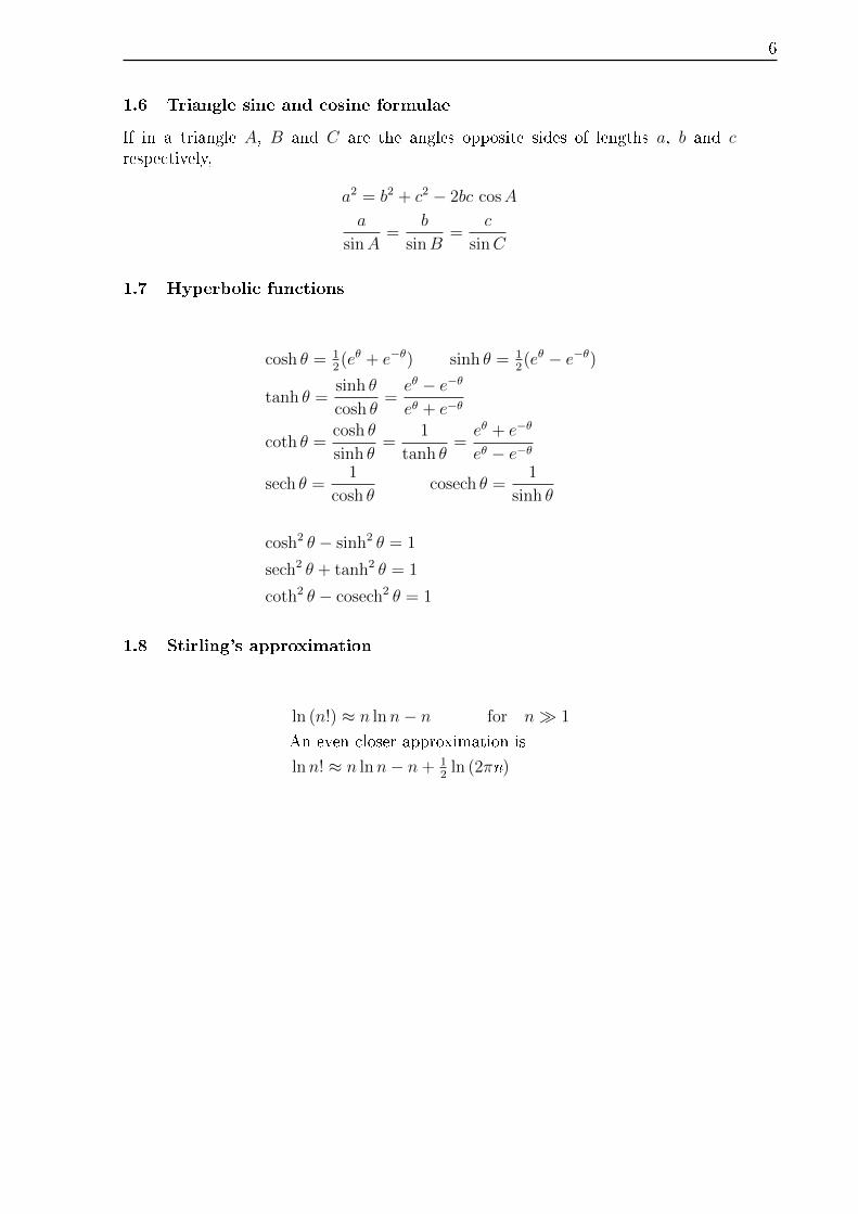
1.6 Triangle sine and cosine formulae
If in a triangle A, B and C are the angles opposite sides of lengths a, b and crespectively,
a2 = b2 + c2 − 2bc cosA
a
sinA=
b
sinB=
c
sinC
1.7 Hyperbolic functions
cosh θ = 12(eθ + e−θ) sinh θ = 1
2(eθ − e−θ)
tanh θ =sinh θ
cosh θ=eθ − e−θeθ + e−θ
coth θ =cosh θ
sinh θ=
1
tanh θ=eθ + e−θ
eθ − e−θ
sech θ =1
cosh θcosech θ =
1
sinh θ
cosh2 θ − sinh2 θ = 1
sech2 θ + tanh2 θ = 1
coth2 θ − cosech2 θ = 1
1.8 Stirling's approximation
ln (n!) ≈ n lnn− n for n� 1
An even closer approximation is
lnn! ≈ n lnn− n+ 12
ln (2πn)
7
2 SERIES FORMULAE
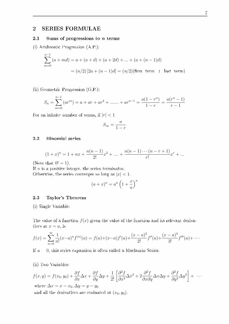
2.1 Sums of progressions to n terms
(i) Arithmetic Progression (A.P.):
n−1∑m=0
(a+md) = a+ (a+ d) + (a+ 2d) + ...+ (a+ (n− 1)d)
= (n/2) [2a+ (n− 1)d] = (n/2)(�rst term + last term)
(ii) Geometric Progression (G.P.):
Sn =n−1∑m=0
(arm) = a+ ar + ar2 + .......+ arn−1 =a(1− rn)
1− r =a(rn − 1)
r − 1
For an in�nite number of terms, if |r| < 1
S∞ =a
1− r
2.2 Binomial series
(1 + x)n = 1 + nx+n(n− 1)
2!x2 + ....+
n(n− 1) · · · (n− r + 1)
r!xr + ...
(Note that 0! = 1).If n is a positive integer, the series terminates.Otherwise, the series converges so long as |x| < 1.
(a+ x)n = an(
1 +x
a
)n2.3 Taylor's Theorem
(i) Single Variable:
The value of a function f(x) given the value of the function and its relevant deriva-tives at x = a, is
f(x) =∞∑n=0
1
n!(x−a)nf (n)(a) = f(a)+(x−a)f ′(a)+
(x− a)2
2!f ′′(a)+
(x− a)3
3!f ′′′(a)+ · · ·
If a = 0, this series expansion is often called a Maclaurin Series.
(ii) Two Variables:
f(x, y) = f(x0, y0) +∂f
∂x∆x+
∂f
∂y∆y +
1
2!
[∂2f
∂x2∆x2 + 2
∂2f
∂x∂y∆x∆y +
∂2f
∂y2∆y2
]+ · · ·
where ∆x = x− x0,∆y = y − y0and all the derivatives are evaluated at (x0, y0).
8
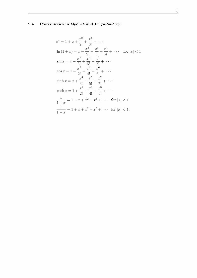
2.4 Power series in algebra and trigonometry
ex = 1 + x+x2
2!+x3
3!+ · · ·
ln (1 + x) = x− x2
2+x3
3− x4
4+ · · · for |x| < 1
sinx = x− x3
3!+x5
5!− x7
7!+ · · ·
cosx = 1− x2
2!+x4
4!− x6
6!+ · · ·
sinhx = x+x3
3!+x5
5!+x7
7!+ · · ·
coshx = 1 +x2
2!+x4
4!+x6
6!+ · · ·
1
1 + x= 1− x+ x2 − x3 + · · · for |x| < 1.
1
1− x = 1 + x+ x2 + x3 + · · · for |x| < 1.
9
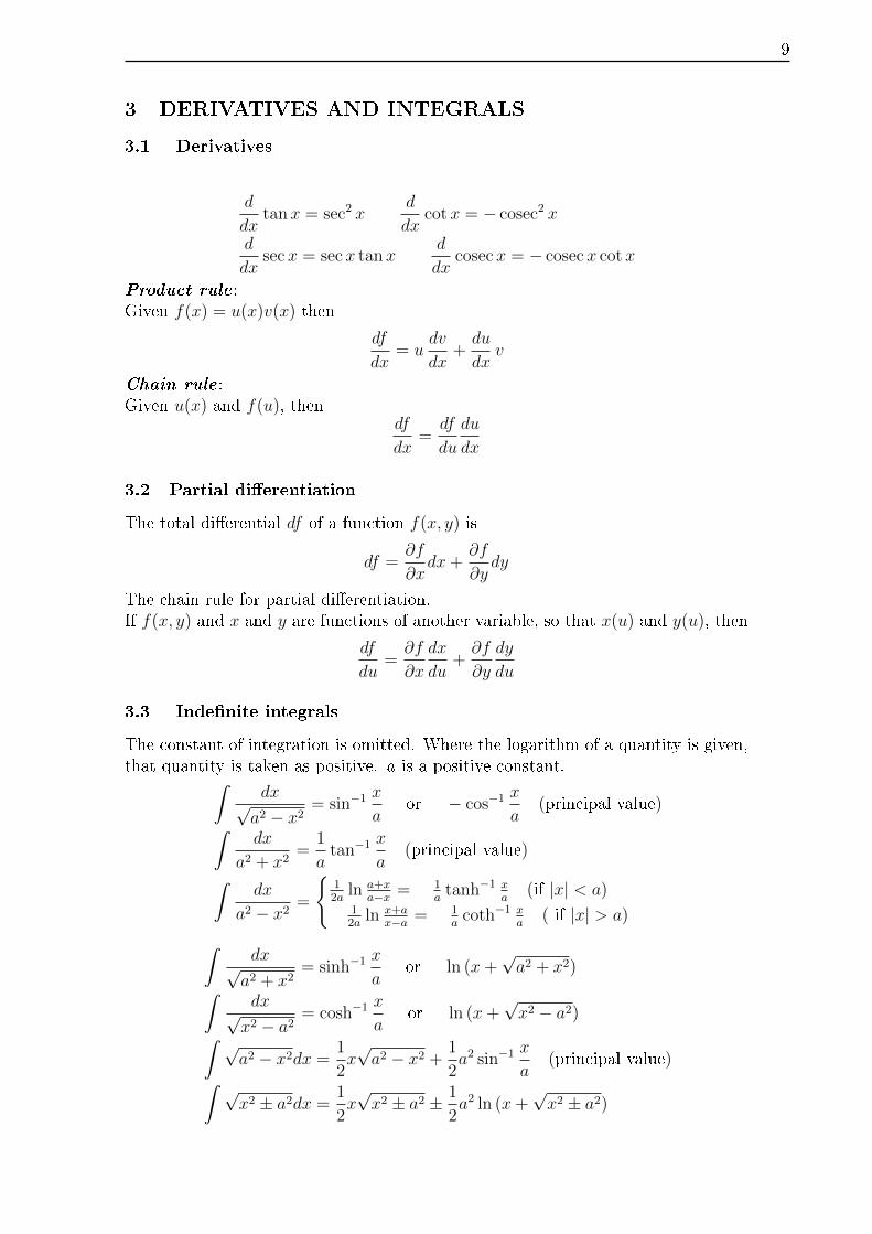
3 DERIVATIVES AND INTEGRALS
3.1 Derivatives
d
dxtanx = sec2 x
d
dxcotx = − cosec2 x
d
dxsecx = secx tanx
d
dxcosecx = − cosecx cotx
Product rule :Given f(x) = u(x)v(x) then
df
dx= u
dv
dx+du
dxv
Chain rule :Given u(x) and f(u), then
df
dx=df
du
du
dx
3.2 Partial di�erentiation
The total di�erential df of a function f(x, y) is
df =∂f
∂xdx+
∂f
∂ydy
The chain rule for partial di�erentiation.If f(x, y) and x and y are functions of another variable, so that x(u) and y(u), then
df
du=∂f
∂x
dx
du+∂f
∂y
dy
du
3.3 Inde�nite integrals
The constant of integration is omitted. Where the logarithm of a quantity is given,that quantity is taken as positive. a is a positive constant.ˆ
dx√a2 − x2
= sin−1x
aor − cos−1
x
a(principal value)
ˆdx
a2 + x2=
1
atan−1
x
a(principal value)
ˆdx
a2 − x2 =
{12a
ln a+xa−x = 1
atanh−1 x
a(if |x| < a)
12a
ln x+ax−a = 1
acoth−1 x
a( if |x| > a)
ˆdx√a2 + x2
= sinh−1x
aor ln (x+
√a2 + x2)
ˆdx√x2 − a2
= cosh−1x
aor ln (x+
√x2 − a2)
ˆ √a2 − x2dx =
1
2x√a2 − x2 +
1
2a2 sin−1
x
a(principal value)
ˆ √x2 ± a2dx =
1
2x√x2 ± a2 ± 1
2a2 ln (x+
√x2 ± a2)
10
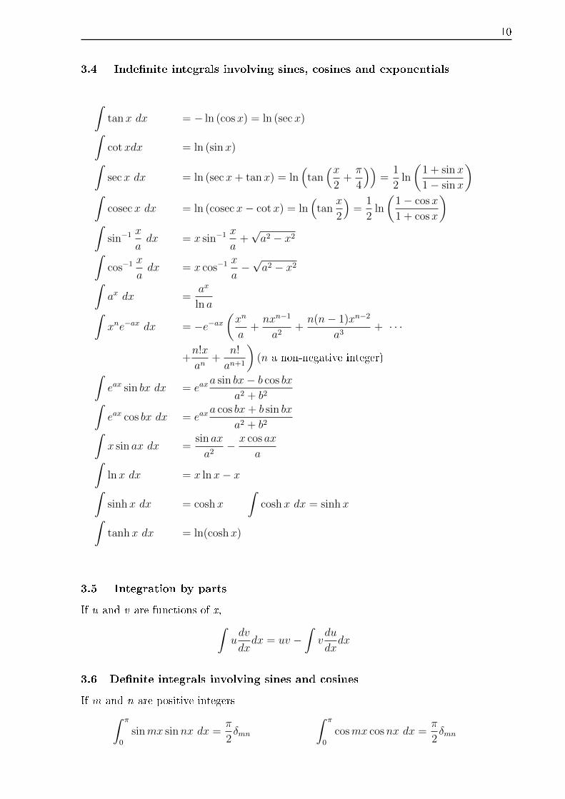
3.4 Inde�nite integrals involving sines, cosines and exponentials
ˆtanx dx = − ln (cosx) = ln (secx)
ˆcotxdx = ln (sin x)
ˆsecx dx = ln (sec x+ tanx) = ln
(tan(x
2+π
4
))=
1
2ln
(1 + sin x
1− sinx
)ˆ
cosecx dx = ln (cosec x− cotx) = ln(
tanx
2
)=
1
2ln
(1− cosx
1 + cos x
)ˆ
sin−1x
adx = x sin−1
x
a+√a2 − x2
ˆcos−1
x
adx = x cos−1
x
a−√a2 − x2
ˆax dx =
ax
ln aˆxne−ax dx = −e−ax
(xn
a+nxn−1
a2+n(n− 1)xn−2
a3+ · · ·
+n!x
an+
n!
an+1
)(n a non-negative integer)
ˆeax sin bx dx = eax
a sin bx− b cos bx
a2 + b2ˆeax cos bx dx = eax
a cos bx+ b sin bx
a2 + b2ˆx sin ax dx =
sin ax
a2− x cos ax
aˆlnx dx = x lnx− x
ˆsinhx dx = coshx
ˆcoshx dx = sinhx
ˆtanhx dx = ln(coshx)
3.5 Integration by parts
If u and v are functions of x,ˆudv
dxdx = uv −
ˆvdu
dxdx
3.6 De�nite integrals involving sines and cosines
If m and n are positive integersˆ π
0
sinmx sinnx dx =π
2δmn
ˆ π
0
cosmx cosnx dx =π
2δmn

11
where
δmn =
{1 if m = n
0 if m 6= n
is the Kronecker delta.
ˆ π/2
−π/2sinmx cosnx dx = 0
3.7 De�nite integrals involving exponentials
ˆ ∞0
x e−αx dx =1
α2ˆ ∞0
e−αx2
dx =1
2
√π
αˆ ∞0
xe−αx2
dx =1
2αˆ ∞0
x2e−αx2
dx =1
4
√π
α3ˆ ∞0
x3e−αx2
dx =1
2α2ˆ ∞0
x4e−αx2
dx =3
8
√π
α5ˆ y
0
e−x2
dx =
√π
2erf(y)
ˆ ∞0
x2 e−αx dx =2
α3ˆ ∞−∞
e−αx2
dx =
√π
αˆ ∞−∞
xe−αx2
dx = 0
ˆ ∞−∞
x2e−αx2
dx =1
2
√π
α3ˆ ∞−∞
x3e−αx2
dx = 0
ˆ ∞−∞
x4e−αx2
dx =3
4
√π
α5ˆ y
0
e−αx2
dx =1
2
√π
αerf(√α y)
3.8 Numerical integration
The interval between a and b is divided into equal intervals h.y has values y0, y1, y2 · · · yn.
12
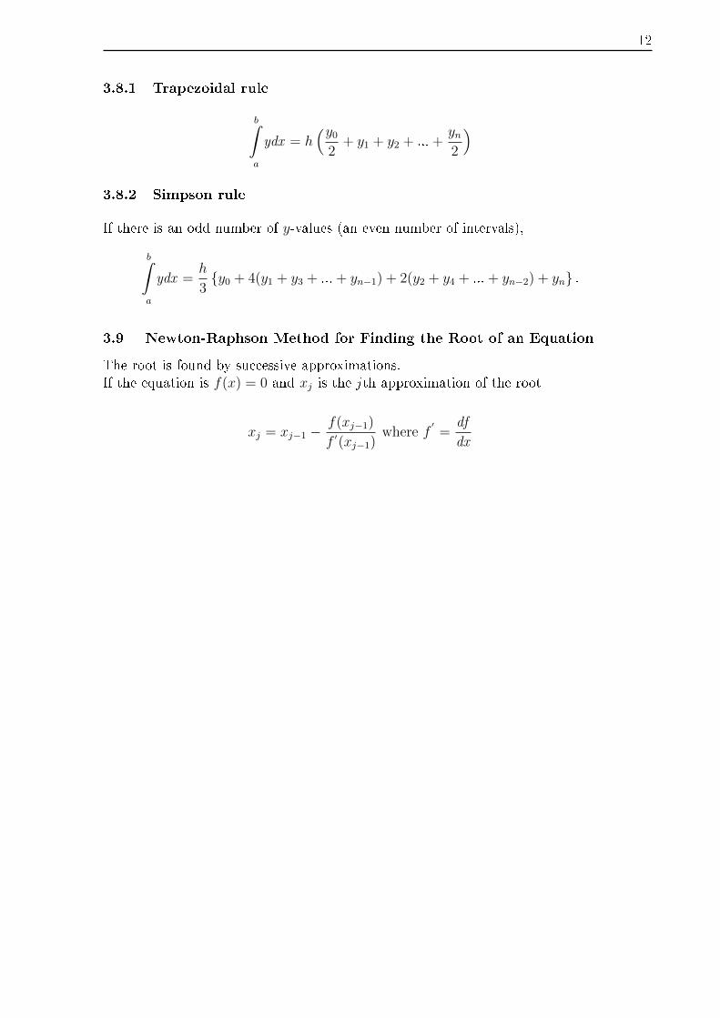
3.8.1 Trapezoidal rule
b
a
ydx = h(y0
2+ y1 + y2 + ... +
yn2
)
3.8.2 Simpson rule
If there is an odd number of y-values (an even number of intervals),
b
a
ydx =h
3{y0 + 4(y1 + y3 + ... + yn−1) + 2(y2 + y4 + ... + yn−2) + yn} .
3.9 Newton-Raphson Method for Finding the Root of an Equation
The root is found by successive approximations.If the equation is f(x) = 0 and xj is the j th approximation of the root
xj = xj−1 −f(xj−1)
f ′(xj−1)where f
′=
df
dx
13
4 COMPLEX NUMBERS
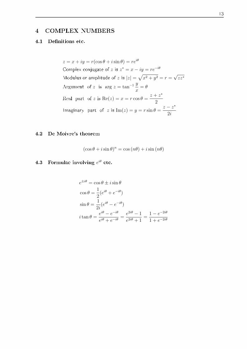
4.1 De�nitions etc.
z = x+ iy = r(cos θ + i sin θ) = reiθ
Complex conjugate of z is z∗ = x− iy = re−iθ
Modulus or amplitude of z is |z| =√x2 + y2 = r =
√zz∗
Argument of z is arg z = tan−1y
x= θ
Real part of z is Re(z) = x = r cos θ =z + z∗
2
Imaginary part of z is Im(z) = y = r sin θ =z − z∗
2i
4.2 De Moivre's theorem
(cos θ + i sin θ)n = cos (nθ) + i sin (nθ)
4.3 Formulae involving eiθ etc.
e±iθ = cos θ ± i sin θ
cos θ =1
2(eiθ + e−iθ)
sin θ =1
2i(eiθ − e−iθ)
i tan θ =eiθ − e−iθeiθ + e−iθ
=e2iθ − 1
e2iθ + 1=
1− e−2iθ1 + e−2iθ
14
5 SPECIAL FUNCTIONS
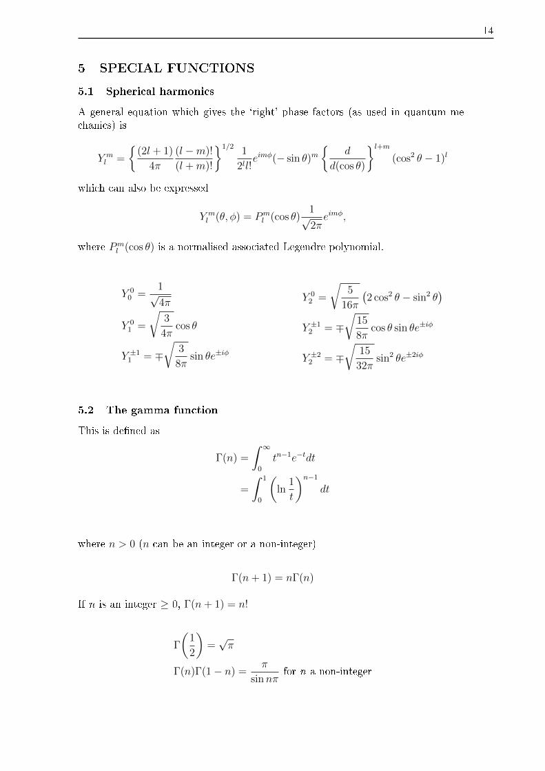
5.1 Spherical harmonics
A general equation which gives the `right' phase factors (as used in quantum me-chanics) is
Y ml =
{(2l + 1)
4π
(l −m)!
(l +m)!
}1/21
2ll!eimφ(− sin θ)m
{d
d(cos θ)
}l+m(cos2 θ − 1)l
which can also be expressed
Y ml (θ, φ) = Pm
l (cos θ)1√2πeimφ,
where Pml (cos θ) is a normalised associated Legendre polynomial.
Y 00 =
1√4π
Y 01 =
√3
4πcos θ
Y ±11 = ∓√
3
8πsin θe±iφ
Y 02 =
√5
16π
(2 cos2 θ − sin2 θ
)Y ±12 = ∓
√15
8πcos θ sin θe±iφ
Y ±22 = ∓√
15
32πsin2 θe±2iφ
5.2 The gamma function
This is de�ned as
Γ(n) =
ˆ ∞0
tn−1e−tdt
=
ˆ 1
0
(ln
1
t
)n−1dt
where n > 0 (n can be an integer or a non-integer)
Γ(n+ 1) = nΓ(n)
If n is an integer ≥ 0, Γ(n+ 1) = n!
Γ
(1
2
)=√π
Γ(n)Γ(1− n) =π
sinnπfor n a non-integer
15
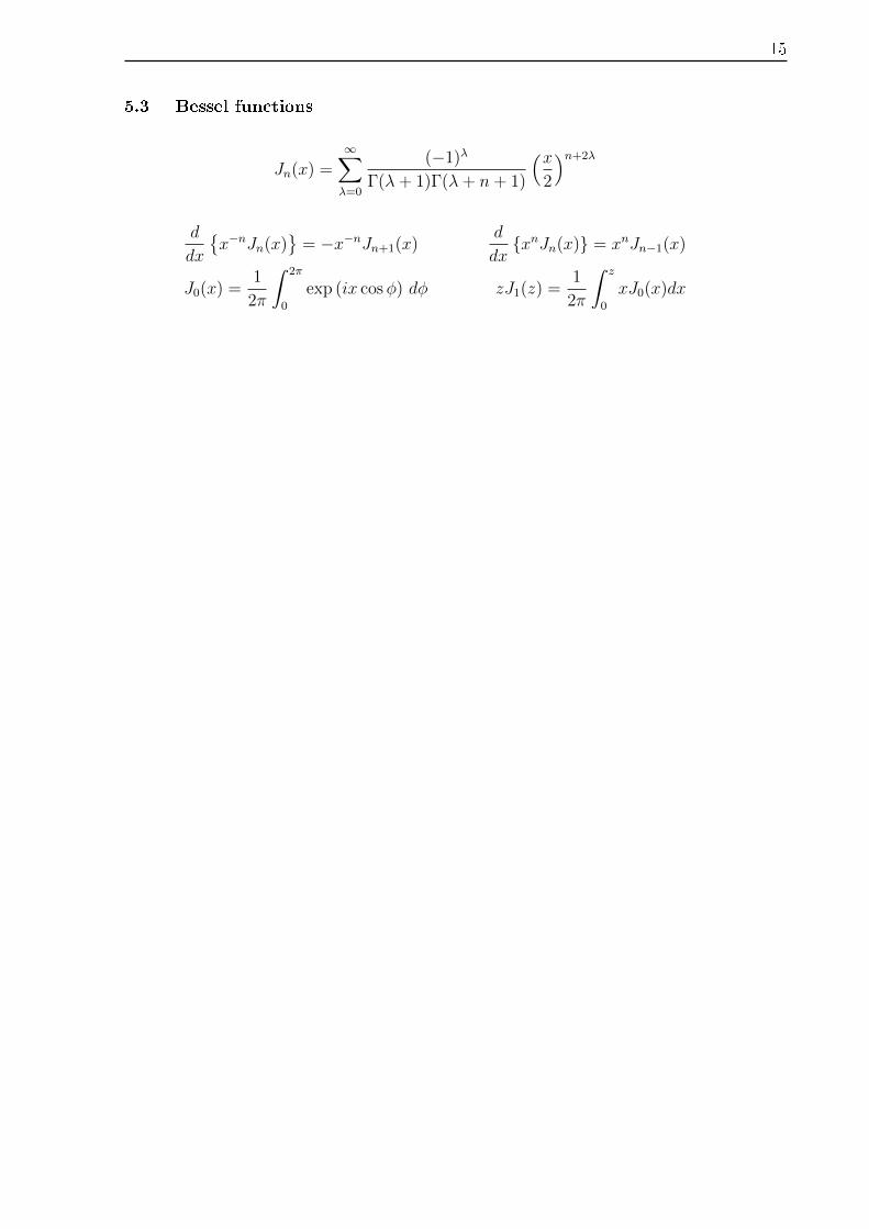
5.3 Bessel functions
Jn(x) =∞∑λ=0
(−1)λ
Γ(λ+ 1)Γ(λ+ n+ 1)
(x2
)n+2λ
d
dx
{x−nJn(x)
}= −x−nJn+1(x)
d
dx{xnJn(x)} = xnJn−1(x)
J0(x) =1
2π
ˆ 2π
0
exp (ix cosφ) dφ zJ1(z) =1
2π
ˆ z
0
xJ0(x)dx
16
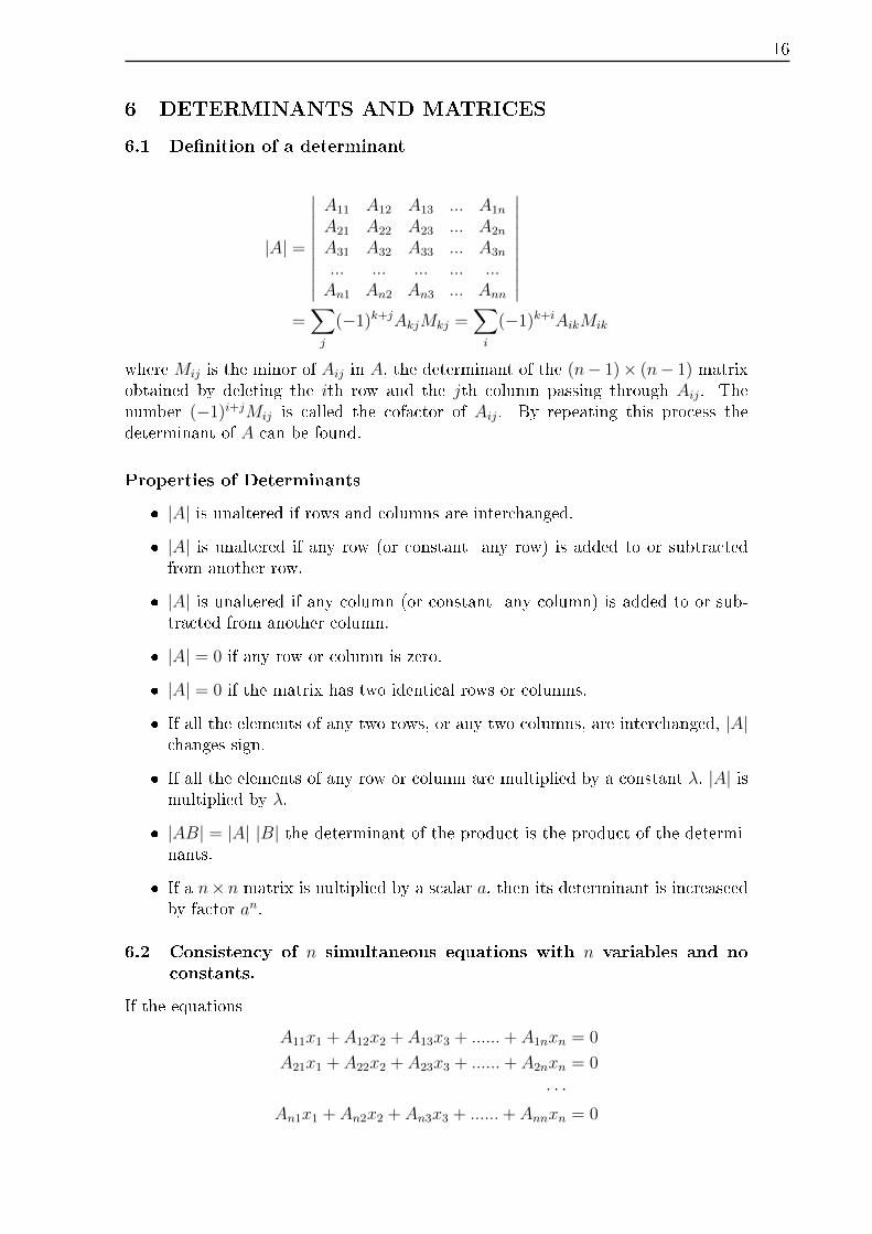
6 DETERMINANTS AND MATRICES
6.1 De�nition of a determinant
|A| =
∣∣∣∣∣∣∣∣∣∣A11 A12 A13 ... A1n
A21 A22 A23 ... A2n
A31 A32 A33 ... A3n
... ... ... ... ...An1 An2 An3 ... Ann
∣∣∣∣∣∣∣∣∣∣=∑j
(−1)k+jAkjMkj =∑i
(−1)k+iAikMik
where Mij is the minor of Aij in A, the determinant of the (n− 1)× (n− 1) matrixobtained by deleting the ith row and the jth column passing through Aij. Thenumber (−1)i+jMij is called the cofactor of Aij. By repeating this process thedeterminant of A can be found.
Properties of Determinants
� |A| is unaltered if rows and columns are interchanged.
� |A| is unaltered if any row (or constant any row) is added to or subtractedfrom another row.
� |A| is unaltered if any column (or constant any column) is added to or sub-tracted from another column.
� |A| = 0 if any row or column is zero.
� |A| = 0 if the matrix has two identical rows or columns.
� If all the elements of any two rows, or any two columns, are interchanged, |A|changes sign.
� If all the elements of any row or column are multiplied by a constant λ, |A| ismultiplied by λ.
� |AB| = |A| |B| the determinant of the product is the product of the determi-nants.
� If a n×n matrix is nultiplied by a scalar a, then its determinant is increaseedby factor an.
6.2 Consistency of n simultaneous equations with n variables and noconstants.
If the equations
A11x1 + A12x2 + A13x3 + ......+ A1nxn = 0
A21x1 + A22x2 + A23x3 + ......+ A2nxn = 0
· · ·An1x1 + An2x2 + An3x3 + ......+ Annxn = 0
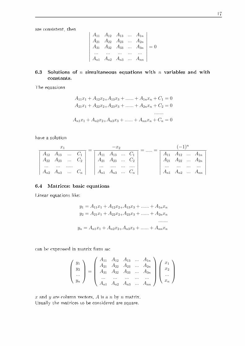
17
are consistent, then ∣∣∣∣∣∣∣∣∣∣A11 A12 A13 ... A1n
A21 A22 A23 ... A2n
A31 A32 A33 ... A3n
... ... ... ... ...An1 An2 An3 ... Ann
∣∣∣∣∣∣∣∣∣∣= 0
6.3 Solutions of n simultaneous equations with n variables and withconstants.
The equations
A11x1 + A12x2+A13x3 + ......+ A1nxn + C1 = 0
A21x1 + A22x2+A23x3 + ......+ A2nxn + C2 = 0
.......
An1x1 + An2x2+An3x3 + ......+ Annxn + Cn = 0
have a solution
x1∣∣∣∣∣∣∣∣A12 A13 ... C1
A22 A23 ... C2
... ... .....An2 An3 ... Cn
∣∣∣∣∣∣∣∣=
−x2∣∣∣∣∣∣∣∣A11 A13 ... C1
A21 A23 ... C2
... .... ... ....An1 An3 ... Cn
∣∣∣∣∣∣∣∣= ..... =
(−1)n∣∣∣∣∣∣∣∣A11 A12 ... A1n
A21 A22 ... A2n
... ... ... ...An1 An2 ... Ann
∣∣∣∣∣∣∣∣6.4 Matrices: basic equations
Linear equations like:
y1 = A11x1 + A12x2+A13x3 + ......+ A1nxn
y2 = A21x1 + A22x2+A23x3 + ......+ A2nxn
.......
yn = An1x1 + An2x2+An3x3 + ......+ Annxn
can be expressed in matrix form as:
y1y2...yn
=
A11 A12 A13 ... A1n
A21 A22 A23 ... A2n
A31 A32 A33 ... A3n
... ... ... ... ...An1 An2 An3 ... Ann
x1x2...xn
x and y are column vectors, A is a n by n matrix.Usually the matrices to be considered are square.
18
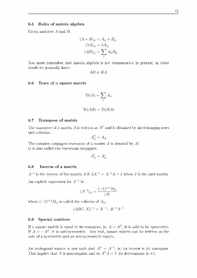
6.5 Rules of matrix algebra
Given matrices A and B,
(A+B)ij = Aij +Bij
(λA)ij = λAij
(AB)ij =∑l
AilBlj
You must remember that matrix algebra is not commutative in general; in otherwords we generally have:
AB 6= BA.
6.6 Trace of a square matrix
Tr(A) =∑i
Aii
Tr(AB) = Tr(BA)
6.7 Transpose of matrix
The transpose of a matrix A is written as AT and is obtained by interchanging rowsand columns.
ATij = Aji
The complex conjugate transpose of a matrix A is denoted by A†.It is also called the Hermitian conjugate.
A†ij = A∗ji
6.8 Inverse of a matrix
A−1 is the inverse of the matrix A if AA−1 = A−1A = I where I is the unit matrix.
An explicit expression for A−1 is:
(A−1)ij =(−1)j+iMji
|A|where (−1)i+jMij is called the cofactor of Aij.
(ABC..X)−1 = X−1...B−1A−1
6.9 Special matrices
If a square matrix is equal to its transpose, ie, A = AT , it is said to be symmetric.If A = −AT , it is anti-symmetric. Any real, square matrix can be written as thesum of a symmetric and an anti-symmetric matrix.
An orthogonal matrix is one such that AT = A−1, ie, its inverse is its transpose.This implies that A is non-singular and as ATA = I, its determinant is ±1.
19
A Hermitian matrix satis�es the relation A = A†. Any complex n by n matrix canbe written as a sum of a Hermitian and an anti-Hermitian matrix.
Unitary matrices have the special property that A† = A−1. Finally, normal matricesare ones that commute with their Hermitian conjugates.
6.10 Eigenvalues and eigenvectors of a square matrix
For a square n × n matrix A there are n eigenvalues λ with associated eigenvaluesx which satisfy:
Ax = λx
x is a vector, which when operated on by A is simply scaled. The eigenvalues aredetermined by �nding the non-trivial solutions of
|A− λI| = 0.
The left-hand side is a polynomial of order n, so this equation � the characteristicequation � has n roots giving the n eigenvalues (which are not necessarily distinct).
6.11 Similarity transform
The operation on a matrix A to produce a matrix B = Q−1AQ is called a similaritytransformation. Under a similarity transform,
TrB = TrA
|B| = |A|
6.12 Diagonalisation of a matrix A with di�erent eigenvalues
If Q is a matrix whose columns are the eigenvectors of a matrix A, then Q−1AQ isdiagonal and has elements which are the eigenvalues of A.
6.13 Representation of a rotation by a matrix R
A real orthogonal 3 × 3 matrix R with determinant = 1 represents a rotation in3-dimensional space.
The angle of implied rotation θ is given by TrR = 1 + 2 cos θ.The axis of implied rotation is a column vector u which is the solution of Ru = u.
20
7 VECTORS
Throughout, i, j and k are unit vectors parallel to Ox, Oy and Oz respectively.
7.1 De�nition of the scalar (or dot) product of two vectors
a · b = |a||b| cos θ (with 0 ≤ θ ≤ π) where θ is the angle between a and b.
7.2 Properties of the scalar product
i · i = j · j = k · k = 1.
i · j = i · k = j · k = 0.
If a · b = 0, and the moduli of a and b are non-zero, then a is perpendicular (or-thogonal) to b.
If a = axi + ayj + azk and b = bxi + byj + bzk,
a · b = axbx + ayby + azbz
a · a = |a|2 = a2x + a2y + a2z
a = (a · i)i + (a · j)j + (a · k)k
7.3 De�nition of the vector (or cross) product of two vectors
a× b = |a||b| sin θn (with 0 ≤ θ ≤ π) where θ is the angle between a and b, andwhere n is the unit vector perpendicular to the plane of a and b and such that a, band n form a right-handed system.
7.4 Properties of the vector product
i× i = j× j = k× k = 0
i× j = k, j× k = i, k× i = j
a× b = −b× a
If a = axi + ayj + azk and b = bxi + byj + bzk,
a× b =
∣∣∣∣∣∣i j kax ay azbx by bz
∣∣∣∣∣∣
21
a× b = |a||b| sin θ is the area of a parallelogram with sides a and b, having anangle θ between the adjacent sides.
a× b = 0 and the moduli of a and b are both non-zero, then a and b are parallelor anti-parallel.
7.5 Scalar triple product
[a b c] = a · (b× c) which also equals (a× b) · c.
[a b c] = [b c a] = [c a b] = − [a c b] = − [b a c] = − [c b a].
If a, b and c are coplanar, then [a b c] = 0.
The volume of a parallelopiped with edges a, b and c is [a b c].
7.6 Vector triple product
a× (b× c) = (a · c)b− (a · b)c
(Note that a× (b× c) 6= (a× b)× c, ie the vector product is not associative.)
7.7 The del operator ∇
∇ = i∂
∂x+ j
∂
∂y+ k
∂
∂z.
7.8 The gradient of a scalar function φ(x, y, z)
grad φ = ∇φ = i∂φ
∂x+ j
∂φ
∂y+ k
∂φ
∂z.
∇φ gives the magnitude and direction of the maximum (spatial) rate of change ofφ.
7.9 The divergence of a vector function F(x, y, z) = Fxi + Fyj + Fzk
div F = ∇ · F =∂Fx∂x
+∂Fy∂y
+∂Fz∂z
div F = i · ∂F∂x
+ j · ∂F∂y
+ k · ∂F∂z
22
7.10 The curl of a vector function F(x, y, z) = Fxi + Fyj + Fzk
curl F = ∇× F = i
(∂Fz∂y− ∂Fy
∂z
)+ j
(∂Fx∂z− ∂Fz
∂x
)+ k
(∂Fy∂x− ∂Fx
∂y
).
curl F = i× ∂F
∂x+ j× ∂F
∂y+ k× ∂F
∂z=
∣∣∣∣∣∣i j k∂∂x
∂∂y
∂∂z
Fx Fy Fz
∣∣∣∣∣∣7.11 Compound operations
div grad φ = ∇ · (∇φ) = ∇2φ =∂2φ
∂x2+∂2φ
∂y2+∂2φ
∂z2
(∇2 is the Laplacian).
div curl F = ∇ · (∇× F) = [∇ ∇ F] = 0.
curl grad φ = ∇× (∇φ) = 0
curl curl F = ∇× (∇× F) = ∇(∇ · F)−∇2F = grad divF−∇2F
where
∇2F =∂2F
∂x2+∂2F
∂y2+∂2F
∂z2
These equations can `deduced' by regarding ∇ as a vector
7.12 Operations on sums and products
∇(φ+ ψ) = ∇φ+∇ψ
∇ · (a + b) = ∇ · a +∇ · b
∇× (a + b) = ∇× a +∇× b
∇(φ ψ) = φ ∇ψ + ψ ∇φ
∇(a · b) = (b · ∇)a + (a · ∇)b + b× (∇× a) + a× (∇× b)
∇ · (φ a) = φ ∇ · a + (∇φ) a
23
∇ · (a× b) = b · ∇ × a− a · ∇ × b
∇× (φ a) = φ ∇× a + (∇φ)× a
∇× (a× b) = (b · ∇)a− (a · ∇)b + a (∇ · b)− b (∇ · a)
7.13 Gauss's (divergence) theorem
Let V be a region, completely bounded by a closed surface S with outward drawnunit normal n. Then, for a well-behaved vector function F(x, y, z)
‹S
F · dS =
˚V
∇ · F dV
where dS = ndS and dS is an element of the surface.
7.14 Stokes's theorem
Let S be a surface with unit normal n, bounded by a closed curve C. Then, for a"well-behaved" vector function F(x, y, z),
˛C
F · dr =
¨S
∇× F · dS
where dr = i dx+ j dy + k dz and dS = ndS.
24
8 CYLINDRICAL AND SPHERICAL POLAR COORDI-
NATES
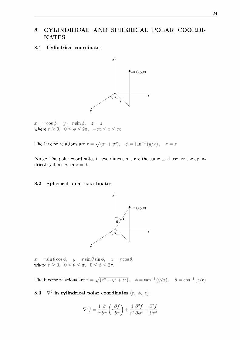
8.1 Cylindrical coordinates
x = r cosφ, y = r sinφ, z = zwhere r ≥ 0, 0 ≤ φ ≤ 2π, −∞ ≤ z ≤ ∞
The inverse relations are r =√
(x2 + y2), φ = tan−1 (y/x) , z = z
Note: The polar coordinates in two dimensions are the same as those for the cylin-drical systems with z = 0.
8.2 Spherical polar coordinates
x = r sin θ cosφ, y = r sin θ sinφ, z = r cos θ.where r ≥ 0, 0 ≤ θ ≤ π, 0 ≤ φ ≤ 2π.
The inverse relations are r =√
(x2 + y2 + z2), φ = tan−1 (y/x) , θ = cos−1 (z/r)
8.3 ∇2 in cylindrical polar coordinates (r, φ, z)
∇2f =1
r
∂
∂r
(r∂f
∂r
)+
1
r2∂2f
∂φ2+∂2f
∂z2
25
8.4 ∇2 in spherical polar coordinates (r, θ, φ)
∇2f =1
r2∂
∂r
(r2∂f
∂r
)+
1
r2 sin θ
∂
∂θ
(sin θ
∂f
∂θ
)+
1
r2 sin2 θ
∂2f
∂φ2
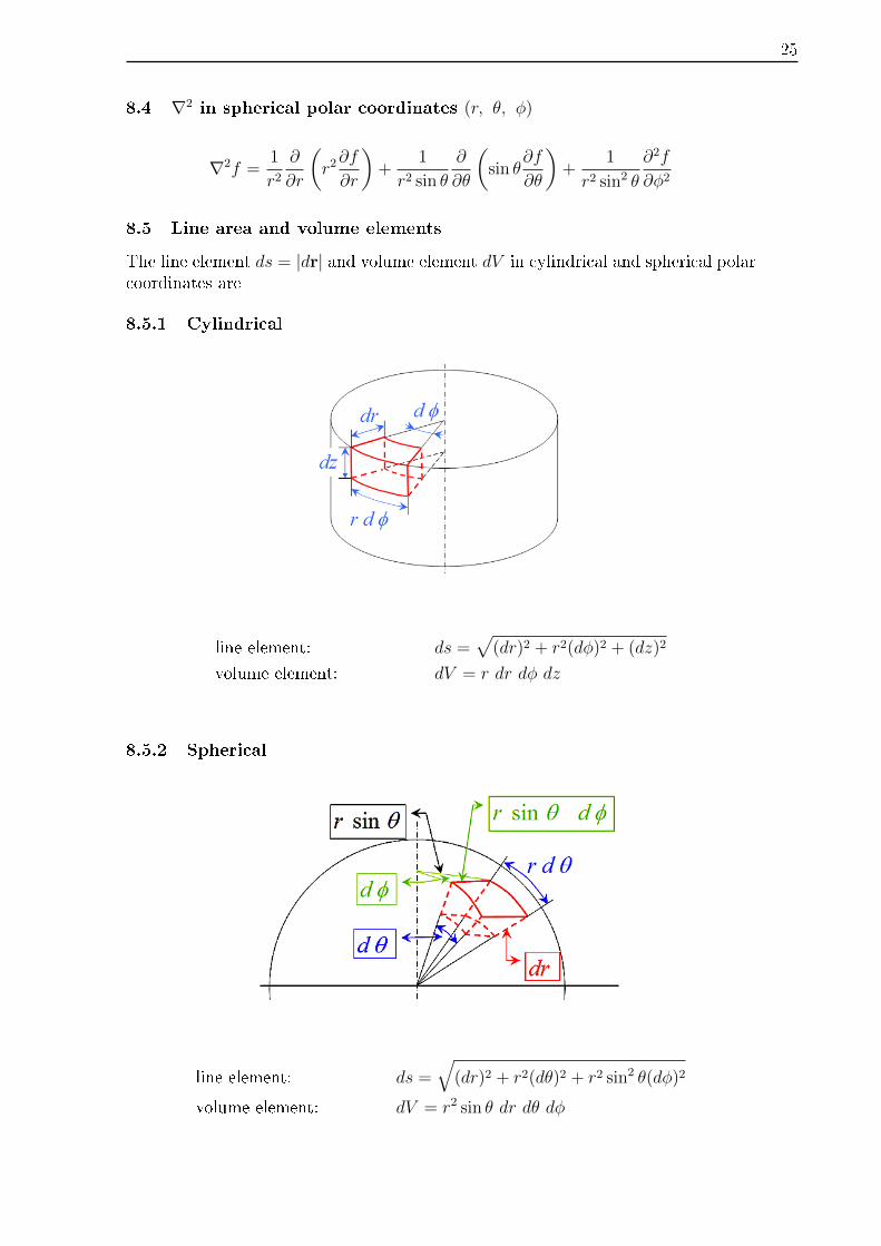
8.5 Line area and volume elements
The line element ds = |dr| and volume element dV in cylindrical and spherical polarcoordinates are
8.5.1 Cylindrical
line element: ds =√
(dr)2 + r2(dφ)2 + (dz)2
volume element: dV = r dr dφ dz
8.5.2 Spherical
line element: ds =√
(dr)2 + r2(dθ)2 + r2 sin2 θ(dφ)2
volume element: dV = r2 sin θ dr dθ dφ

26
9 FOURIER SERIES AND TRANSFORMS
A function f(t) which is periodic in t with period T satis�es f(t+ T ) = f(t).It can be expanded in an in�nite series of exponentials or of sines and cosines.
9.1 Fourier Series
(a) Complex expansion
f(t) =∞∑
n=−∞
Fne−iωnt,
where ωn =2πn
T(n = 0,±1,±2.....∞)
and Fn =1
T
ˆT
eiωntf(t) dt
Here, the integral is taken over one complete period(e.g. from 0 to T or from −T/2 to T/2).Note the orthogonality relation
1
T
ˆT
e−iωnteiωmtdt = δnm
where δnm is the Kronecker delta.
(b) Real expansionBy separating the above result into real and imaginary parts, for real f(t),
f(t) = a0 +∞∑n=1
an cosωnt+ bn sinωnt
where an =2
T
ˆT
f(t) cosωnt dt
bn =2
T
ˆT
f(t) sinωnt dt
and a0 =1
T
ˆT
f(t) dt
9.2 Fourier transforms
By letting T → ∞ and replacing sums by integrals, one �nds that (suitably re-stricted) functions f(t) can be expressed as a `superposition' of exponential func-tions.
f(t) =1
2π
ˆ ∞−∞
F (ω)e−iωtdω
where F (ω) =
ˆ ∞−∞
f(t)eiωtdt
The functions f(t) and F (ω) are `Fourier mates', and the results can be viewed asa consequence of the fact thatˆ ∞
−∞e−iωteiω
′t dt = 2πδ(ω − ω′)
27
9.3 Shift theorems in Fourier transforms
(a) If f(t) is replaced by f(t− a) (ie. a translation in time by a),
F (ω) is replaced by F (ω)eiωa
(b) If f(t) is multiplied by eiω′t
F (ω) is ‘translated′ into F (ω + ω′)
9.4 Convolutions
If f(t) and g(t) are two functions, their convolution (with respect to t) h(t), isde�ned by
h(t) = f(t) ∗ g(t) =
ˆ ∞−∞
f(u)g(t− u)du
=
ˆ ∞−∞
f(t− u)g(u)du
The Fourier transform of h(t) is H(ω) = F (ω)G(ω), where F (ω) and G(ω) are theFourier transforms of f(t) and g(t).
Similarly, H(ω) = F (ω) ∗G(ω) is the Fourier transform of h(t) = f(t)g(t)
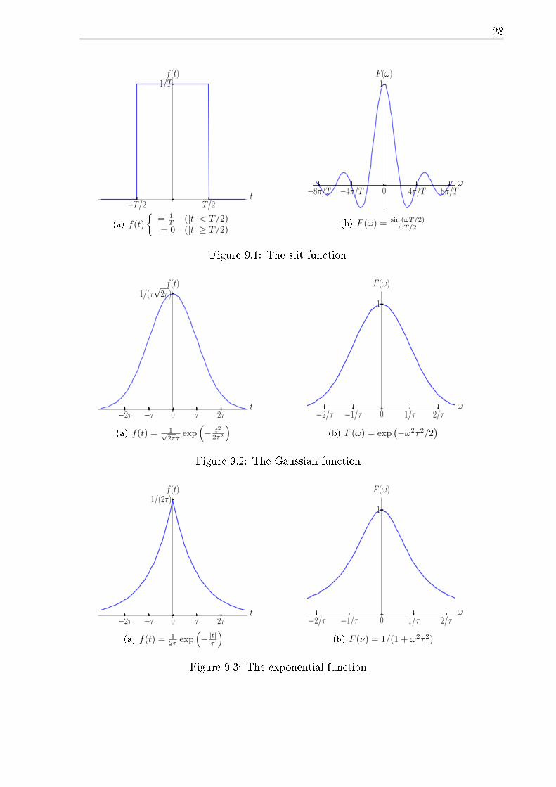
9.5 Some common Fourier mates
f(t) =1
2π
ˆ ∞−∞
F (ω)e−iωtdω F (ω) =
ˆ ∞−∞
f(t)eiωtdt
f(t) = e−iω0t F (ω) = 2πδ(ω − ω0)
f(t) = sinω0t F (ω) =π
i[δ(ω + ω0)− δ(ω − ω0)]
f(t) = cosω0t F (ω) = π [δ(ω + ω0) + δ(ω − ω0)]
f(t) = δ(t− t0) F (ω) = eiωt0
28
−T/2 T/2t
1/Tf (t)
(a) f(t)
{= 1
T (|t| < T/2)= 0 (|t| ≥ T/2)
−8π/T −4π/T 0 4π/T 8π/Tω
1F (ω)
(b) F (ω) = sin (ωT/2)ωT/2
Figure 9.1: The slit function
−2τ −τ 0 τ 2τt
1/(τ√
2π)f (t)
(a) f(t) = 1√2πτ
exp(− t2
2τ2
) −2/τ −1/τ 0 1/τ 2/τω
1
F (ω)
(b) F (ω) = exp(−ω2τ2/2
)Figure 9.2: The Gaussian function
−2τ −τ 0 τ 2τt
1/(2τ )f (t)
(a) f(t) = 12τ exp
(− |t|
τ
) −2/τ −1/τ 0 1/τ 2/τω
1
F (ω)
(b) F (ν) = 1/(1 + ω2τ2)
Figure 9.3: The exponential function

29
9.6 Di�raction at a circular aperture
The integral of e2πiSr cosφ over the area of a circle isˆ 2π
φ=0
ˆ a
r=0
e2πiSr cosφrdrdφ =aJ1(2πSa)
S
-15 -10 -5 5 10 15x
0.1
0.2
0.3
0.4
0.5J1(x)/x
J1(x)
x= when |x| = 1.22π(= 3.3833), 2.233π(= 7.016), 3.238π(= 10.174), ...
= max. when |x| = 0, 2.679π(= 8.417), ...
= min. when |x| = 1.635π(= 5.136), 3.699π(= 11.620), ...
30
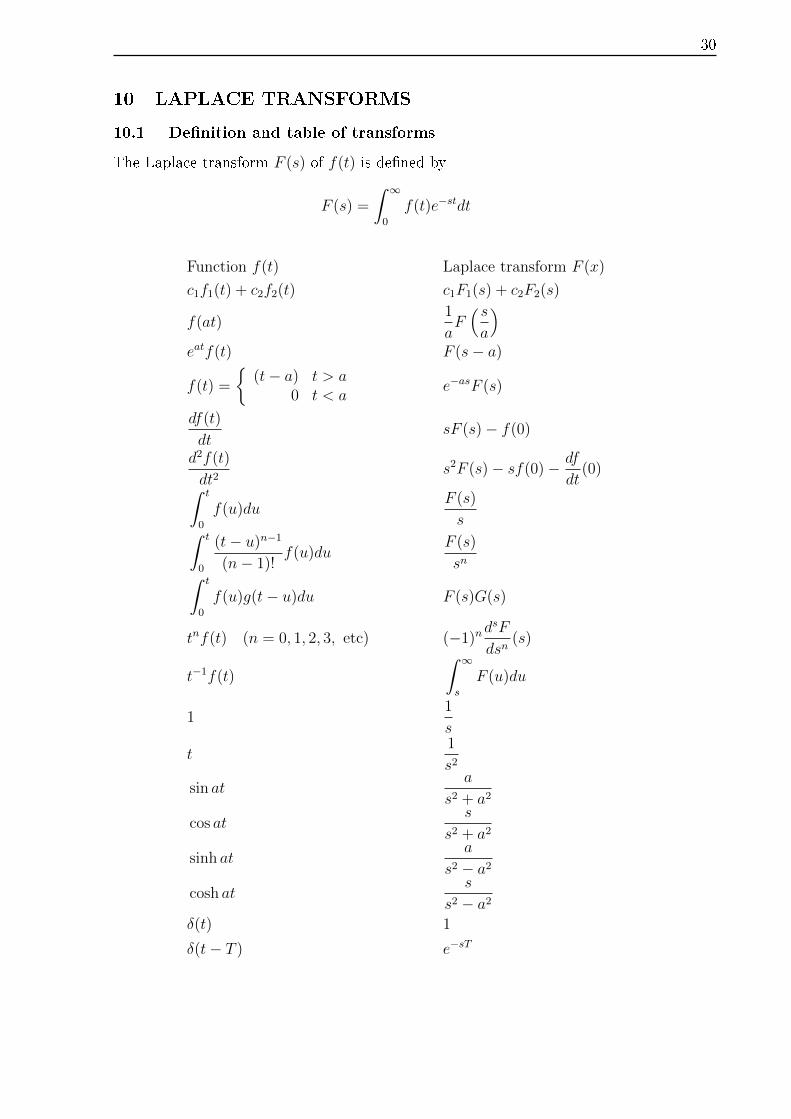
10 LAPLACE TRANSFORMS
10.1 De�nition and table of transforms
The Laplace transform F (s) of f(t) is de�ned by
F (s) =
ˆ ∞0
f(t)e−stdt
Function f(t) Laplace transform F (x)
c1f1(t) + c2f2(t) c1F1(s) + c2F2(s)
f(at)1
aF(sa
)eatf(t) F (s− a)
f(t) =
{(t− a) t > a
0 t < ae−asF (s)
df(t)
dtsF (s)− f(0)
d2f(t)
dt2s2F (s)− sf(0)− df
dt(0)
ˆ t
0
f(u)duF (s)
sˆ t
0
(t− u)n−1
(n− 1)!f(u)du
F (s)
snˆ t
0
f(u)g(t− u)du F (s)G(s)
tnf(t) (n = 0, 1, 2, 3, etc) (−1)ndsF
dsn(s)
t−1f(t)
ˆ ∞s
F (u)du
11
s
t1
s2
sin ata
s2 + a2
cos ats
s2 + a2
sinh ata
s2 − a2cosh at
s
s2 − a2δ(t) 1
δ(t− T ) e−sT

31
11 PROBABILITY, STATISTICS AND DATA INTERPRE-
TATION
11.1 Mean and variance
(a) Discretely distributed random variables (variates)
For a variate x which can take on the N values, xi (i = 1, .... N) with respectiveprobabilities fi,
n∑i=1
fi = 1
Mean of x is x =n∑i=1
fixi
Variance of x is σ2 = Var(x) = (x− x)2 = x2 − x2 =n∑i=1
fix2i − x2
where σ is the standard deviation.
(b) Continuously distributed variates
For a continuously distributed variate x, with probability density function f(x),normalised asˆ ∞
−∞f(x)dx = 1
x =
ˆ ∞−∞
xf(x)dx
Var(x) =
ˆ ∞−∞
(x− x)2f(x)dx =
ˆ ∞−∞
x2f(x)dx− x2 = x2 − x2
(c) Scale factor and change of origin
If y = k(x− a), where k and a are constants, then
y = k(x− a) and
Var(y) = k2Var(x)
11.2 Binomial distribution
In n identical independent trials with probability, p, of success (and q = 1 − p offailure) at each trial, the probability of exactly r successes is
nCrprqn−r =
n!
r!(n− r)!prqn−r
32
Mean number of successes, r = np.
Variance of number of successes Var(r) = npq.
Variance of proportion successes = Var( rn
)=pq
n.
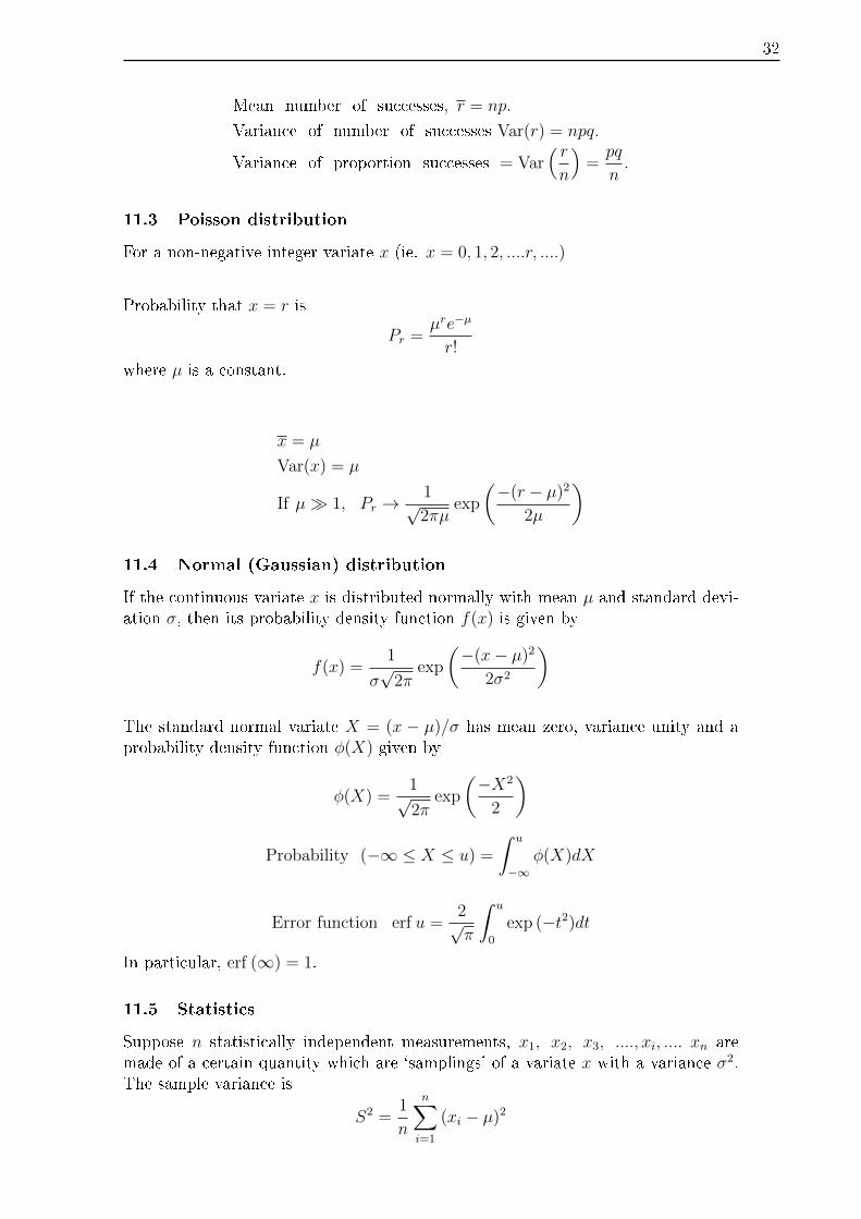
11.3 Poisson distribution
For a non-negative integer variate x (ie. x = 0, 1, 2, ....r, ....)
Probability that x = r is
Pr =µre−µ
r!
where µ is a constant.
x = µ
Var(x) = µ
If µ� 1, Pr →1√2πµ
exp
(−(r − µ)2
2µ
)
11.4 Normal (Gaussian) distribution
If the continuous variate x is distributed normally with mean µ and standard devi-ation σ, then its probability density function f(x) is given by
f(x) =1
σ√
2πexp
(−(x− µ)2
2σ2
)
The standard normal variate X = (x − µ)/σ has mean zero, variance unity and aprobability density function φ(X) given by
φ(X) =1√2π
exp
(−X2
2
)
Probability (−∞ ≤ X ≤ u) =
ˆ u
−∞φ(X)dX
Error function erf u =2√π
ˆ u
0
exp (−t2)dt
In particular, erf (∞) = 1.
11.5 Statistics
Suppose n statistically independent measurements, x1, x2, x3, ...., xi, .... xn aremade of a certain quantity which are `samplings' of a variate x with a variance σ2.The sample variance is
S2 =1
n
n∑i=1
(xi − µ)2
33
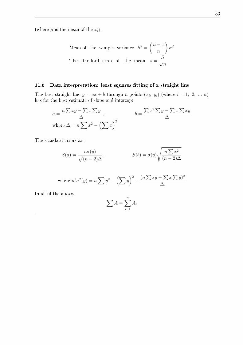
(where µ is the mean of the xi).
Mean of the sample variance S2 =
(n− 1
n
)σ2
The standard error of the mean s =S√n
11.6 Data interpretation: least squares �tting of a straight line
The best straight line y = ax + b through n points (xi, yi) (where i = 1, 2, ... n)has for the best estimate of slope and intercept
a =n∑xy −∑x
∑y
∆, b =
∑x2∑y −∑x
∑xy
∆
where ∆ = n∑
x2 −(∑
x)2
The standard errors are
S(a) =nσ(y)√(n− 2)∆
, S(b) = σ(y)
√n∑x2
(n− 2)∆
where n2σ2(y) = n∑
y2 −(∑
y)2− (n
∑xy −∑x
∑y)2
∆.
In all of the above, ∑A =
n∑i=1
Ai
.
34
12 SOME PHYSICS FORMULAE
12.1 Newton's laws and conservation of energy and momentum
The frictional force f = µFN where FN is the normal force.
The centripetal force is mv2/r = mω2r.
The work done by a force:´Fdx or force × dist for a constant force.
The mechanical energy = K + U is conserved.
Conservation of momentum: (∑
imivi)init = (∑
imivi)final.
For rocket motion: vf − vi = vrel ln (mi/mf ).
12.2 Rotational motion and angular momentum
Angular speed ω = v/r.
The rotational inertia is I =∑mir
2i .
For mass M rotating about an axis distance R away, I = MR2.
Newton's second (angular) law is net torque, τnet = Iα and τ = r× F.
For a rolling ball, K = Krot +Ktrans = 0.5Iω2 + 0.5mv2com.For a wheel (radius R) rolling smoothly: vcom = ωR.
Angular momentum L = mr× v.
Angular momentum L = Iω is conserved.
12.3 Gravitation and Planetary motion
Gravitational force: F = GmMr/r3
Gravitational law in di�erential form: ∇ · g = −4πGρ
Gravitational potential energy is U = −GMm/r.
Escape speed : v =√
2GM/R.
Kepler's second law: A = L/2M = constant.
Kepler's third law: T 2 = (4π2/GM)r3.
12.4 Oscillations - Simple harmonic motion, Springs
Spring restoring force: F = −kx.Displacement : x = xm cos (ωt+ φ), where ω2 = k/m.
Period T = 2π√m/k = 2π/ω
Energy: K = mx2/2, U = kx2/2.
35
12.5 Thermodynamics, gases and �uids
Change in heat energy is ∆Q = mc∆T .
Heat of transformation ∆Q = Lm.
Ideal gas equation of state: pV = nRT .
1st law of thermodynamics : dEint = dQ− dW .Also ∆Eint = ∆Eint,f −∆Eint,i = Q−W .For cyclical processes: ∆Eint = 0, Q = W .
Work done: W =´dW =
´pdV
For an isothermal process W = nRT lnVf/Vi.
root mean square velocity is vrms =√
(3RT/M) where M is the molecular mass.
Maxwell-Boltzmann distribution
f(v) = 4π
(m
2πkBT
)3/2
v2 exp −(mv2
2kBT
)where v is the velocity and m the mass of the each particle.
Bernoulli's equation for the �ow of an ideal �uid
p
ρ+
1
2v2 + gz = constant
12.6 Waves
Wave equation∂2y
∂x2=
1
v2∂2y
∂t2
The speed of the wave v = fλ where λ is the wavelength and f is the frequency.The angular frequency ω = 2πf .
Energy of one photon: E = hf = hc/λ
Photoelectric e�ect equation: eV0 = hf − φ.φ is the workfunction of the surface and V0 is the applied voltage.
Speed of electromagnetic waves: c = 1/√ε0µ0
Index of refraction: n = c/v
Snell's law of refraction between media a and b: na sin θa = nb sin θb
Constructive interference: d sin θ = mλ
Destructive interference: d sin θ = (m+ 1/2)λ
Transverse wave in a string of tension T and mass/length µ: v =√T/µ
Longitudinal wave in a �uid of density ρ and bulk modulus B: v =√B/ρ
36
12.7 Electricity and Magnetism
Coulomb's LawF =
1
4πε0
q1q2r2
Electric �eldE =
1
4πε0
q
r2r
Potential di�erence
Va − Vb =
ˆ b
a
E · dr
12.8 Maxwell's equations
Integral form Di�erential form
Gauss' law for electricity‹
E · dS =
∑qi
ε0=Q
ε0∇ · E =
ρ
ε0
Gauss' law for magnetism‹
B · dS = 0 ∇ ·B = 0
Faraday's law˛E · dr = −dΦB
dt∇× E = −∂B
∂t
Ampere-Maxwell law˛B · dr =
1
c2dΦE
dt+ µ0I ∇×B =
1
c2∂E
∂t+ µ0j
12.9 Special Relativity
Lorentz contraction : L = L0/γ where γ = 1/√
(1− v2/c2).time dilation : ∆t = γ∆t0.
Lorentz transformation eqns:x′ = γ(x− vt), t′ = γ(t− vx/c2), y′ = y and z′ = z.
Relativistic momentum p = γmv.
Relativistic energy E = mc2 +K = γmc2.
Relativistic energy equation: E2 = (pc)2 + (mc2)2.
37
12.10 Photons, atoms and quantum mechanics
Photons: E = hf , p = h/λ.
Photoelectric equation: hf = Kmax + Φ, where Φ is the work function.
Compton scattering: ∆λ = h(1− cosφ)/mc.
Heisenberg uncertainty principle: ∆px∆x ≥ ~/2
A particle with momentum p has de Broglie wavelength: λ = h/p
The Schrödinger equation
One-dimension: − ~2
2m
d2ψ(x)
dx2+ V (x)ψ(x) = Eψ(x)
Three dimension: − ~2
2m
[∂2
∂x2+
∂2
∂y2+
∂2
∂z2
]ψ(r) + V (r)ψ(r) = Eψ(r)
Hyrogen atom: − ~2
2m∇2u(r)− e2
4πε0ru(r) = Eu(r)
The energy levels of a particle (mass m) in an in�nite square well of width L aregiven by
En =h2
8mL2n2.
The electron energy levels in the hydrogen atom are:
En = −13.6
n2eV.
The probability of �nding a particle, described by a wavefunction ψ(x), betweenpositions x = a and x = b is P =
´ ba|ψ(x)|2 dx.
The wavelength of radiation absorbed/emitted by an electron going from energylevel Ei to Ef is
1
λ= R∞
[1
n2i
− 1
n2f
]where R∞ is the Rydberg constant.
The transmission coe�cient for a particle of mass m tunnelling across a barrier ofheight V and width L is
T = e−2bL where b =
√8π2m(V − E)
~2
Fermi-Dirac distribution: f(E) = [exp {(E − µ)/kBT}+ 1]−1
Bose-Einstein distribution: f(E) = [exp {(E − µ)/kBT} − 1]−1
38
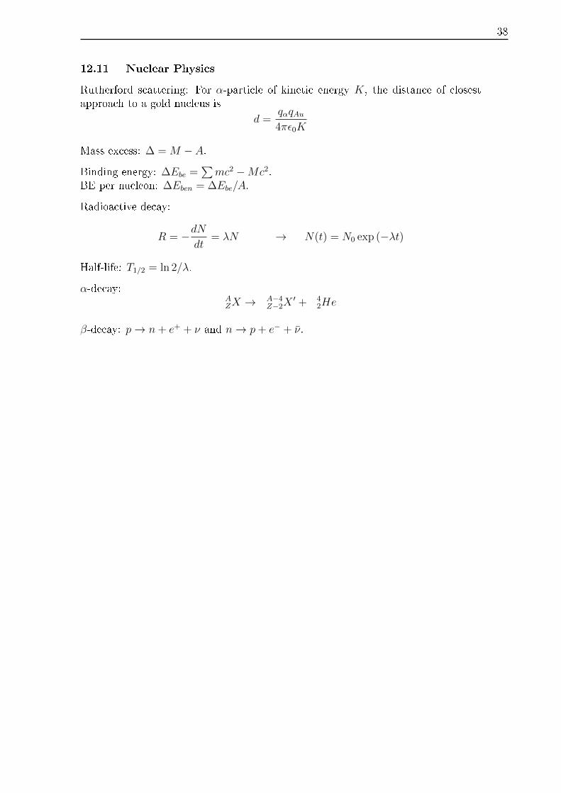
12.11 Nuclear Physics
Rutherford scattering: For α-particle of kinetic energy K, the distance of closestapproach to a gold nucleus is
d =qαqAu4πε0K
Mass excess: ∆ = M − A.Binding energy: ∆Ebe =
∑mc2 −Mc2.
BE per nucleon: ∆Eben = ∆Ebe/A.
Radioactive decay:
R = −dNdt
= λN → N(t) = N0 exp (−λt)
Half-life: T1/2 = ln 2/λ.
α-decay:AZX → A−4
Z−2X′ + 4
2He
β-decay: p→ n+ e+ + ν and n→ p+ e− + ν.
39
13 PHYSICAL CONSTANTS AND CONVERSIONS
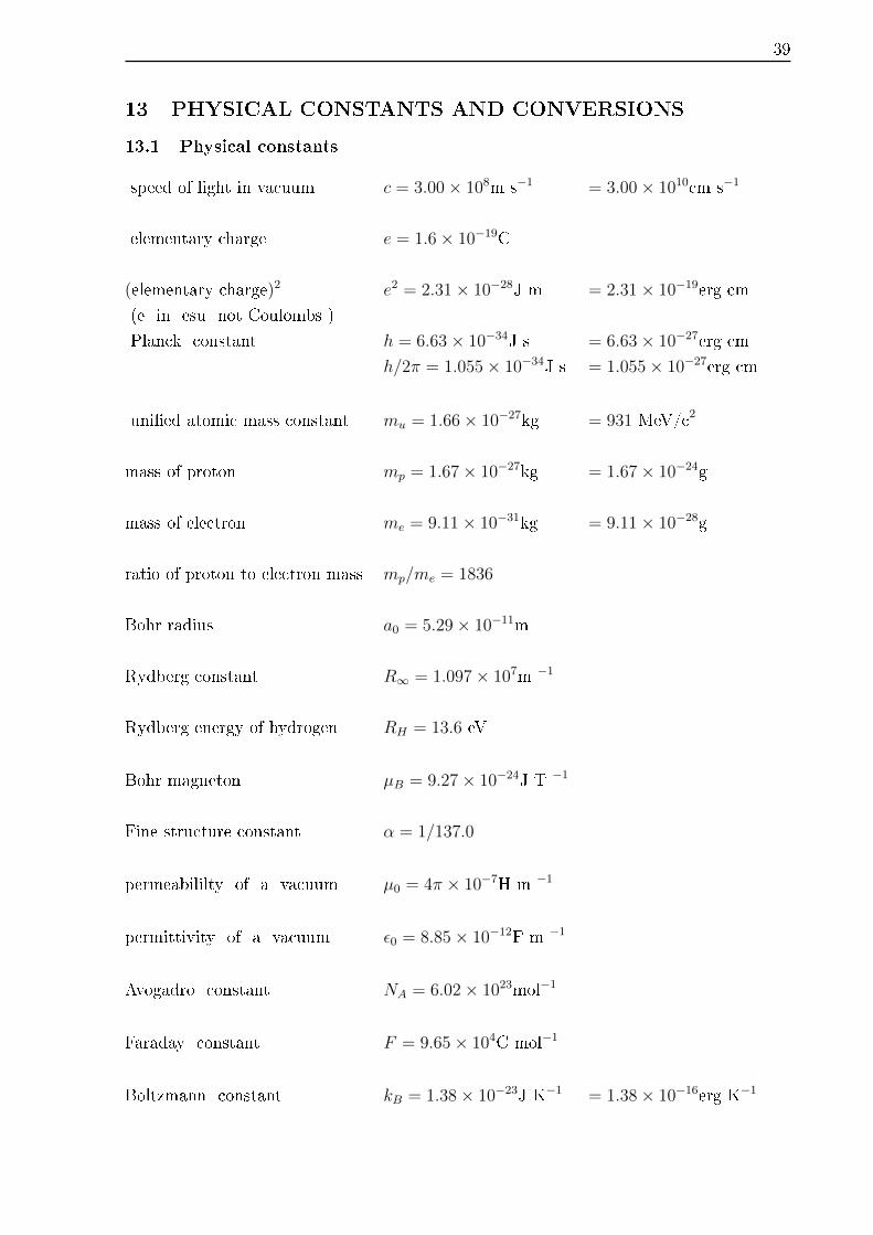
13.1 Physical constants
speed of light in vacuum c = 3.00× 10⁸m s−1 = 3.00× 1010cm s−1
elementary charge e = 1.6× 10⁻¹⁹C
(elementary charge)2 e2 = 2.31× 10⁻²⁸J m = 2.31× 10⁻¹⁹erg cm
(e in esu not Coulombs )
Planck constant h = 6.63× 10⁻³⁴J s = 6.63× 10⁻²⁷erg cm
h/2π = 1.055× 10⁻³⁴J s = 1.055× 10⁻²⁷erg cm
uni�ed atomic mass constant mu = 1.66× 10⁻²⁷kg = 931 MeV/c2
mass of proton mp = 1.67× 10⁻²⁷kg = 1.67× 10⁻²⁴g
mass of electron me = 9.11× 10⁻³¹kg = 9.11× 10⁻²⁸g
ratio of proton to electron mass mp/me = 1836
Bohr radius a0 = 5.29× 10⁻¹¹m
Rydberg constant R∞ = 1.097× 10⁷m −1
Rydberg energy of hydrogen RH = 13.6 eV
Bohr magneton µB = 9.27× 10⁻²⁴J T −1
Fine structure constant α = 1/137.0
permeabililty of a vacuum µ0 = 4π × 10−7H m −1
permittivity of a vacuum ε0 = 8.85× 10⁻¹²F m −1
Avogadro constant NA = 6.02× 10²³mol−1
Faraday constant F = 9.65× 10⁴C mol−1
Boltzmann constant kB = 1.38× 10⁻²³J K−1 = 1.38× 10⁻¹⁶erg K−1

40
gas constant R = 8.31 J K−1mol−1
Stefan-Boltzmann constant σSB = 5.67× 10⁻⁸J s−1m−2K−4 = 5.67× 10⁻⁵erg s−1cm−2K−4
Gravitational constant G = 6.67× 10⁻¹¹m3kg−1s−2 = 6.67× 10⁻⁸cm3g−1s−2
acceleration of free fall g = 9.81m s−2
radiant energy density const a = 7.56× 10⁻¹⁶J m−3K−4 = 7.56× 10⁻¹⁵erg cm−3K−4
13.2 Astronomical constants
Mass associated with one hydrogen m = 2.38× 10⁻²⁴g = 2.38× 10⁻²⁷kg
nucleus for cosmic composition
Solar mass M� = 1.99× 1033g = 1.99× 1030kg
Solar radius R� = 6.96× 1010cm = 6.96× 10⁸m
Earth mass M⊕ = 6.0× 1027g = 6.0× 1024kg
Earth radius R⊕ = 6.4× 108cm = 6.4× 10⁶m
Solar luminosity L� = 3.83× 1033erg s−1 = 3.83× 1026J s−1
Astronomical unit AU = 1.50× 1013cm = 1.50× 10¹¹m
Parsec pc = 3.09× 1018cm = 3.09× 10¹⁶m
13.3 Conversions
1 km = 103 m = 105 cm
1Å (angström unit) = 10−10 m = 10−8 cm
1 year = 3.16× 10⁷ s
1 eV = 1.6× 10⁻¹⁹ J
Celsius temperature = thermodynamic temperature - 273.15