Carbon Footprint of High Speed Railway
58
Carbon Footprint of High Speed Rail
description
Carbon Footprint of High Speed Railway
Transcript of Carbon Footprint of High Speed Railway
Carbon Footprint of High Speed Rail

ii
iii
Carbon Footprint of High Speed Rail
Carbon Footprint of High Speed Rail
Final Report – 1 st of March 2011
- Report -
Paris, November 2011
iv
Authors
T. Baron, G. Martinetti and D. Pépion
Edited and reviewed by
M. Tuchschmid (independent consultant)
This report has been produced by Systra for the UIC High Speed and Sustainable Development Departments. It has been edited and independently reviewed by M. Tuchschmid (independent consultant).
Citation of this report:
T. Baron (SYSTRA), M. Tuchschmid, G. Martinetti and D. Pépion (2011), High Speed Rail and Sustainability. Background Report: Methodology and results of carbon footprint analysis, International Union of Railways (UIC), Paris, 2011.
v
Carbon Footprint of High Speed Rail
Summary
Many carbon footprint tools such as the two UIC tools, EcoTransIT and EcoPassenger 1 , help costumers choose the most environmental friendly way of transport, which in most cases is rail. Until now, these calculation tools have considered only the operation phase and energy provision, not the infrastructure (track system, motorways, airports) nor the construction of rolling stock, cars and aeroplanes. So, the question remains: Does the picture change if we also consider the CO2-emission from the construction of vehicles, and from construction?
This study attempts to answer this question, by providing a carbon footprint analysis of four new high speed rail lines: “LGV Mediterranée” from Valence to Marseille and “South Europe Atlantic-Project” in France from Tours to Bordeaux, the newly built line from Taipei to Kaohsiung in Taiwan and “Beijing–Tianjin” in China.
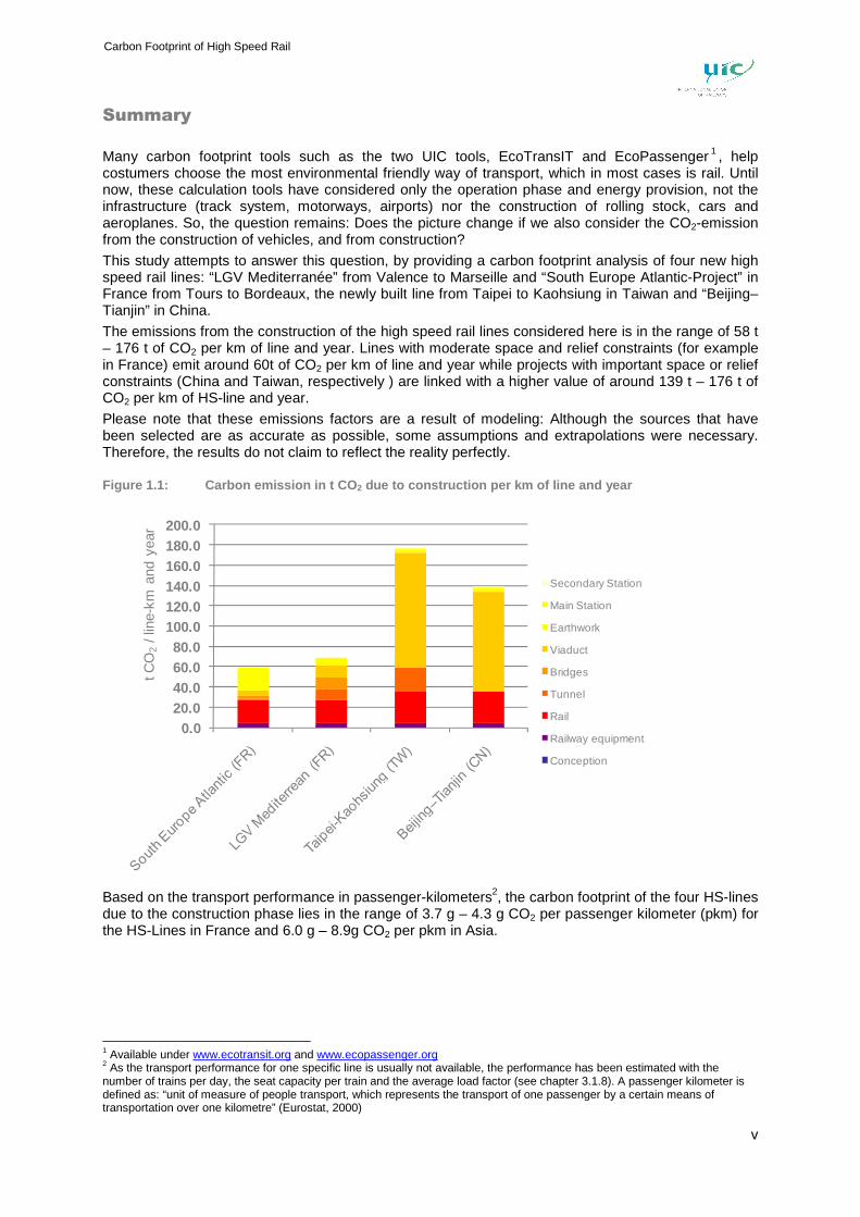
The emissions from the construction of the high speed rail lines considered here is in the range of 58 t – 176 t of CO2 per km of line and year. Lines with moderate space and relief constraints (for example in France) emit around 60t of CO2 per km of line and year while projects with important space or relief constraints (China and Taiwan, respectively ) are linked with a higher value of around 139 t – 176 t of CO2 per km of HS-line and year.
Please note that these emissions factors are a result of modeling: Although the sources that have been selected are as accurate as possible, some assumptions and extrapolations were necessary. Therefore, the results do not claim to reflect the reality perfectly.
Figure 1.1: Carbon emission in t CO 2 due to construction per km of line and year
0.020.040.060.080.0
100.0120.0140.0160.0180.0200.0
Secondary Station
Main Station
Earthwork
Viaduct
Bridges
Tunnel
Rail
Railway equipment
Conception
t CO
2/ l
ine-
km a
nd y
ear
Based on the transport performance in passenger-kilometers2, the carbon footprint of the four HS-lines due to the construction phase lies in the range of 3.7 g – 4.3 g CO2 per passenger kilometer (pkm) for the HS-Lines in France and 6.0 g – 8.9g CO2 per pkm in Asia.
1 Available under www.ecotransit.org and www.ecopassenger.org 2 As the transport performance for one specific line is usually not available, the performance has been estimated with the number of trains per day, the seat capacity per train and the average load factor (see chapter 3.1.8). A passenger kilometer is defined as: “unit of measure of people transport, which represents the transport of one passenger by a certain means of transportation over one kilometre” (Eurostat, 2000)
vi
In a next step, the emissions from the construction of rolling stock and the operation of the railway has been modeled and added to the carbon footprint of the construction.
Table 1.1: Carbon Footprint of High Speed transporta tion services
S-E Atlantic LGV Mediterranée Taipei-Kaohsiung Beijing–Tianjin
Construction 3.7 g CO2 / pkm 4.3 g CO2 / pkm 8.9 g CO2 / pkm 6.0 g CO2 / pkm
Rolling Stock 0.9 g CO2 / pkm 1.0 g CO2 / pkm 0.9 g CO2 / pkm 0.8 g CO2 / pkm
Operation 5.7 g CO2 / pkm 5.7 g CO2 / pkm 42.9 g CO2 / pkm 39.2 g CO2 / pkm
Grand sum 10.4 g CO2 / pkm 11.0 g CO 2 / pkm 52.7 g CO 2 / pkm 46.0 g CO 2 / pkm
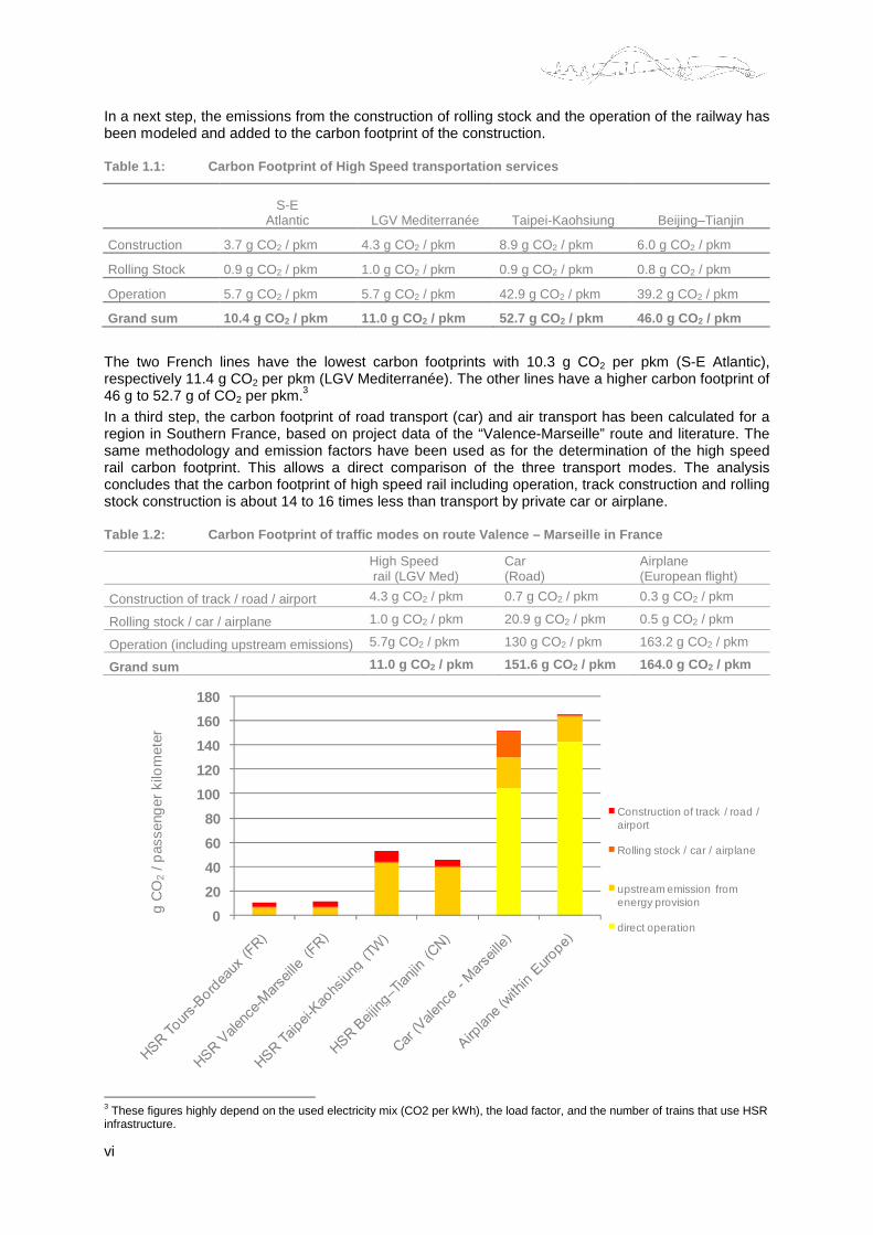
The two French lines have the lowest carbon footprints with 10.3 g CO2 per pkm (S-E Atlantic), respectively 11.4 g CO2 per pkm (LGV Mediterranée). The other lines have a higher carbon footprint of 46 g to 52.7 g of CO2 per pkm.3 In a third step, the carbon footprint of road transport (car) and air transport has been calculated for a region in Southern France, based on project data of the “Valence-Marseille” route and literature. The same methodology and emission factors have been used as for the determination of the high speed rail carbon footprint. This allows a direct comparison of the three transport modes. The analysis concludes that the carbon footprint of high speed rail including operation, track construction and rolling stock construction is about 14 to 16 times less than transport by private car or airplane.
Table 1.2: Carbon Footprint of traffic modes on rou te Valence – Marseille in France
High Speed rail (LGV Med)
Car (Road)
Airplane (European flight)
Construction of track / road / airport 4.3 g CO2 / pkm 0.7 g CO2 / pkm 0.3 g CO2 / pkm
Rolling stock / car / airplane 1.0 g CO2 / pkm 20.9 g CO2 / pkm 0.5 g CO2 / pkm
Operation (including upstream emissions) 5.7g CO2 / pkm 130 g CO2 / pkm 163.2 g CO2 / pkm
Grand sum 11.0 g CO2 / pkm 151.6 g CO 2 / pkm 164.0 g CO 2 / pkm
0
20
40
60
80
100
120
140
160
180
Construction of track / road / airport
Rolling stock / car / airplane
upstream emission from energy provision
direct operation
g C
O2
/ pas
seng
er k
ilom
eter
3 These figures highly depend on the used electricity mix (CO2 per kWh), the load factor, and the number of trains that use HSR infrastructure.
vii
Carbon Footprint of High Speed Rail
In a last step, the environmental benefit of the newly built high speed line “LGV Mediterranée” has been calculated. According to a detailed study4 1.78 million passengers used the high speed train “LGV Med” instead of the airplane for a journey to / from Southern France in the year 2004. This is equal to a transport performance of 1,068 million passenger kilometers. An additional 0.98 million passengers would have taken the car instead of the train.
Table 1.3: Avoided emissions through the constructi on of the “LGV Mediterranée”, considered is the whole TGV-network
Passengers Travel Distance5
Transport performance Emission factor Avoided emissions
[Number] [km] [pkm] [g of CO2 per pkm] [t of CO2 per year] Additional TGV Traffic in 2004 compared to 2000 4,461,000 600 2,676,600,000 0.011 29,461
From air (before) -1,780,000 600 -1,068,000,000 0.1632 -174,298
From road (before) -1,190,000 600 -714,000,000 0.13 -92,820
Grand sum -237,657
For this example the emission factor in France of 91 g of CO2 per kWh and a load factor of 70% for the LGV have been used. This allows the calculation of the environmental benefit through the construction of the new high speed line: Thanks to the construction of the “LGV Mediterranean” about 237,600 t of CO2 can be avoided each year.
This example shows that with the construction of new high speed lines, countries may significantly reduce their transport carbon emissions.
4 RFF (2007 p.75) 5 We assume that travel distance for air and road passengers are equivalent to the distance for rail passengers. In reality, the distance for air passengers is likely to be higher than the travelled distance by rail and the distance for cars passengers lower.
viii
Table of content
1.1 Life cycle assessment in transportation area 1
1.2 Goal of this study 1
1.3 Structure of this report 2
2.1 System boundaries and considered phases 3
2.2 Data sources 4
2.3 Modeling principles 5
2.3.1 Lifespan of considered elements 5
2.3.2 Modeling the components of High Speed line 6
2.3.3 Functional Unit 8
2.3.4 Allocation of infrastructure to the transport of passengers and transport of goods 8
2.3.5 Assumption on temporal scope 8
2.3.6 No consideration of deforestation 8
2.3.7 Cut-off criteria 8
3.1 Carbon footprint of the track construction 9
3.1.1 Emissions from planning phase 9
3.1.2 Emissions from earthworks 9
3.1.3 Emissions from the track construction (ballasted track and concrete slab track) 11
3.1.4 Emissions from civil engineering structures: Viaduct and Bridges 12
3.1.5 Emissions from civil engineering structures: Tunnels 13
3.1.6 Emissions from railway equipments (energy & telecommunication) 15
3.1.7 Emissions from station and technical centers (only construction) 16
3.1.8 Carbon footprint of the construction of selected High Speed lines 17
3.1.9 Conclusion 24
3.2 Carbon Footprint of High Speed rolling stock 27
3.2.1 Emissions from construction, maintenance and disposal of rolling stock 27
3.2.2 Carbon footprint of the rolling stock of selected High Speed lines 28
3.3 Carbon Footprint of High Speed operation 29
3.4 Summary: Carbon Footprint of High Speed transportation services 30
4.1 Comparison of transport services 33
4.1.1 Carbon Footprint of high speed rail transport 33
4.1.2 Carbon Footprint of road transport 33
4.1.3 Carbon Footprint of air transport 34
4.2 Environmental benefit 34
4.2.1 Change of the modal split due to High speed line 34
4.2.2 Methodology of calculation 34
4.2.3 Avoided emissions due to the high speed line 35
4.2.4 “Pay back time” of the emissions due to the LGV-construction 35
5.1 Carbon Footprint of the transport by car 37
5.1.1 Construction / maintenance and disposal 37
5.1.2 Operation of a car 37
5.1.3 Road construction 37
5.2 Carbon Footprint of Air traffic 40
5.2.1 Construction of Airplane 40
5.2.2 Operation of the Airplane 41
5.2.3 Construction of Airport 41
5.3 Carbon Footprint of Electricity generation in selected countries 43
5.4 Bibliography 45
1 INTRODUCTION 1
2 METHODOLOGY 3
3 CARBON FOOTPRINT OF HIGH SPEED LINES 9
4 CASE STUDY “SOUTH FRANCE”: A MODAL COMPARISON 32
5 ANNEX 37
1
Carbon Footprint of High Speed Rail
1 Introduction
Many carbon footprint tools allow a comparison between different transport modes. UIC has itself developed two such tools - EcoPassenger for passenger transport in Europe and EcoTransIT for freight transport worldwide6. Both tools consider the environmental effects of the operation phase including energy provision, but don’t’ take the infrastructure for the track system nor the rolling stock into account.
This study investigates the carbon footprint of selected, new high speed rail lines, including the assessment of the track system and the rolling stock.
1.1 Life cycle assessment in transportation area
Several studies have been carried out in order to assess the entire life cycle impact of transportation systems. Please see below a non exhaustive list:
� Schmied & Mottschall (2010) worked out a detailed study about the carbon footprint of the German rail network. This includes an analysis of the different kind of tracks (different rails and sleepers), the regional variation of the density of trains and a differentiation of local and long-distance traffic.
� Tuchschmid (2010) worked out for UIC a methodology for assessing High Speed Rail. This included an online calculator for assessing high speed rail traffic under different conditions regarding electricity-mix, track usage, load factor and topography reasons. According to the study, the most important factor besides the electricity mix and load factor is the share of bridges and tunnels.
� RFF & SNCF (2009) carried out a detailed Life Cycle Assessment for the new Rhine Rhone High Speed Line.
� G. Martinetti (2008) for SYSTRA assessed the carbon balance of the French East High Speed Line, considering the impact of construction and operation phases, including the environmental benefit from a changing modal split. According to this study, High Speed Rail may effectively reduce CO2-emissions.
� Lee et al. (2008) carried out a study in order to estimate and compare the life cycle impact of ballasted track and slab track in South Korean High Speed Line. This study not only presented materials used in track construction but also assessed construction vehicles activity trough oil consumption.
� Chester et al. (2008) make a Life Cycle Assessment and modal comparison of a large number of transportation systems in the United States of air, road and rail transport. This study also includes the environmental impacts through financial exchange, elaborated with a hybrid LCA methodology.
� Kato et al. (2005) evaluated the impact of interregional high speed mass transit projects in Japan, including Tokaïdo Shinkansen, Maglev trains and planes.
� Von Rozycki et al. (2003) investigated the environmental impact of the German High Speed Line Hannover – Wurzburg. This comprehensive study showed that the operation phase is responsible for about 80% of the environmental footprint.
� Yukizawa et al. (2002) investigated the environmental impact of the construction phase of the Tokaïdo Shinkansen railway.
� Maibach et al. (1999) elaborated a study about traffic modes in Switzerland, which mainly is the basis for the ecoinvent-database (Spielmann, 2007).
1.2 Goal of this study
The present study has three aims:
� First this report compiles an exhaustive and detailed carbon footprint of the construction of new High Speed Rail lines.
� Second, the study will identify and compare the main emissions sources of the lines in roder to highlight the reasons for differences between different high speed lines.
� The third and last step provides a comparison with other modes of transport and the calculation of the environmental benefit due to the newly built high speed line in Southern
6 Available at www.ecotransit.org and www.ecopassenger.org
2
France. This step also includes the impacts of a modal shift from road and air to the new rail line.
1.3 Structure of this report
The structure of this study follows the goals described above. In chapter 0 the methodology and data sources for the elaborated carbon footprint are described.
Chapter 3 provides a carbon footprint analysis of the construction of the different elements of a High speed line, and then highlights the variations between HS lines using a representative sample:
� The “SE-Atlantic” between Tours and Bordeaux (France), � The “LGV Mediterranée” from Valence to Marseille (France), � Taipei-Kaohsiung (Taiwan) and � Beijing–Tianjin (China).
The carbon footprint of the track infrastructure is then combined with the carbon footprint of the rolling stock and the operation phase.
In chapter 3, a comparison is made between the French A7 motorway, the LGV Mediterranée and Marseille Provence airport, all of them located in the same corridor.
3
Carbon Footprint of High Speed Rail
Methodology
The determination of the greenhouse gas emissions has been carried out using an orienting material flow analysis, as a detailed life cycle assessment is beyond the scope of this study. The methods used in the material flow analysis are in line with product category rules for rail infrastructure and rail vehicles. These PCR (Product Category Rules) are in close connection with the ISO standard 14025 (environmental declarations) and the ISO standard 14040 (Life Cycle Assessment). Please note that the comparison in Chapter 3 does not follow the ISO-scheme.
1.4 System boundaries and considered phases
The analysis of the impact of High Speed Lines has been carried out “from cradle to grave”. This includes the construction, operation, maintenance and end-of-life of the high speed rail life cycle. Additionally, the conception and planning stages have been taken into account in order to give a comprehensive overview of the project’s life cycle. Table 1.1 gives an overview of the processes considered.
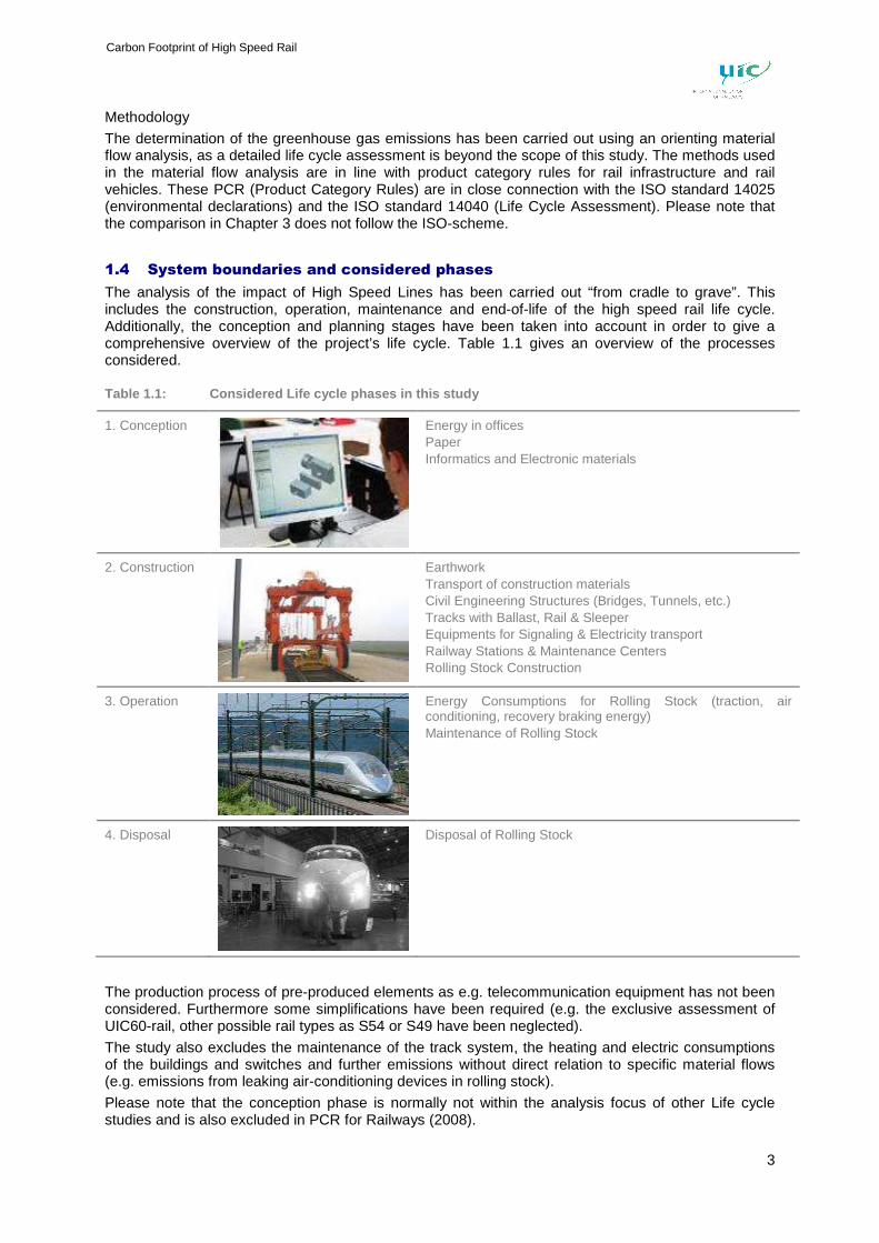
Table 1.1: Considered Life cycle phases in this stu dy
1. Conception
Energy in offices Paper Informatics and Electronic materials
2. Construction
Earthwork Transport of construction materials Civil Engineering Structures (Bridges, Tunnels, etc.) Tracks with Ballast, Rail & Sleeper Equipments for Signaling & Electricity transport Railway Stations & Maintenance Centers Rolling Stock Construction
3. Operation
Energy Consumptions for Rolling Stock (traction, air conditioning, recovery braking energy) Maintenance of Rolling Stock
4. Disposal
Disposal of Rolling Stock
The production process of pre-produced elements as e.g. telecommunication equipment has not been considered. Furthermore some simplifications have been required (e.g. the exclusive assessment of UIC60-rail, other possible rail types as S54 or S49 have been neglected).
The study also excludes the maintenance of the track system, the heating and electric consumptions of the buildings and switches and further emissions without direct relation to specific material flows (e.g. emissions from leaking air-conditioning devices in rolling stock).
Please note that the conception phase is normally not within the analysis focus of other Life cycle studies and is also excluded in PCR for Railways (2008).
4
1.5 Data sources
Enhanced project data was collected throughout the SYSTRA-archives, research literature, various reports from UIC and national railways in order to conduct this carbon footprint of high speed rail.
The project data has to be combined with emission factors to calculate the total amount of carbon emissions. Due to its high reliability, transparent documentation and the international usage of its data (inside the rail sector and more broadly7), the ecoinvent database v2.0 has been chosen for the emission factors.
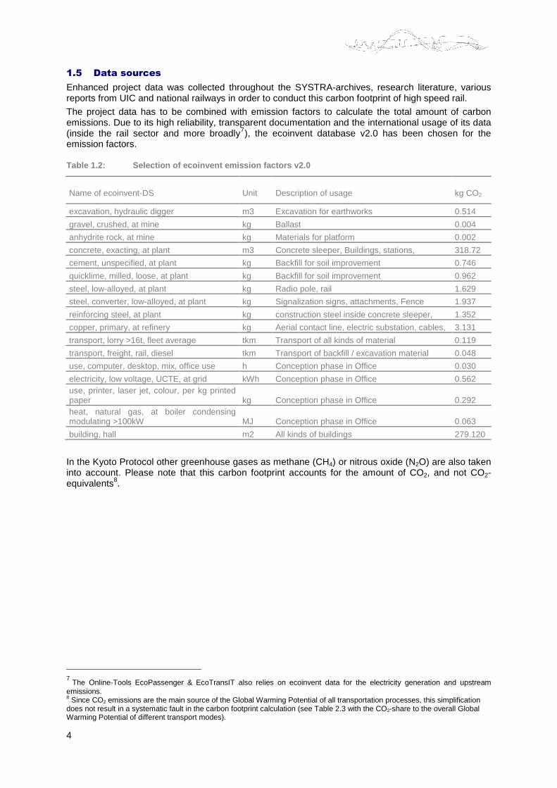
Table 1.2: Selection of ecoinvent emission factors v 2.0
Name of ecoinvent-DS Unit Description of usage kg CO2
excavation, hydraulic digger m3 Excavation for earthworks 0.514
gravel, crushed, at mine kg Ballast 0.004
anhydrite rock, at mine kg Materials for platform 0.002
concrete, exacting, at plant m3 Concrete sleeper, Buildings, stations, 318.72
cement, unspecified, at plant kg Backfill for soil improvement 0.746
quicklime, milled, loose, at plant kg Backfill for soil improvement 0.962
steel, low-alloyed, at plant kg Radio pole, rail 1.629
steel, converter, low-alloyed, at plant kg Signalization signs, attachments, Fence 1.937
reinforcing steel, at plant kg construction steel inside concrete sleeper, 1.352
copper, primary, at refinery kg Aerial contact line, electric substation, cables, 3.131
transport, lorry >16t, fleet average tkm Transport of all kinds of material 0.119
transport, freight, rail, diesel tkm Transport of backfill / excavation material 0.048
use, computer, desktop, mix, office use h Conception phase in Office 0.030
electricity, low voltage, UCTE, at grid kWh Conception phase in Office 0.562 use, printer, laser jet, colour, per kg printed paper kg Conception phase in Office 0.292 heat, natural gas, at boiler condensing modulating >100kW MJ Conception phase in Office 0.063
building, hall m2 All kinds of buildings 279.120
In the Kyoto Protocol other greenhouse gases as methane (CH4) or nitrous oxide (N2O) are also taken into account. Please note that this carbon footprint accounts for the amount of CO2, and not CO2-equivalents8.
7 The Online-Tools EcoPassenger & EcoTransIT also relies on ecoinvent data for the electricity generation and upstream
emissions. 8 Since CO2 emissions are the main source of the Global Warming Potential of all transportation processes, this simplification does not result in a systematic fault in the carbon footprint calculation (see Table 2.3 with the CO2-share to the overall Global Warming Potential of different transport modes).
5
Carbon Footprint of High Speed Rail
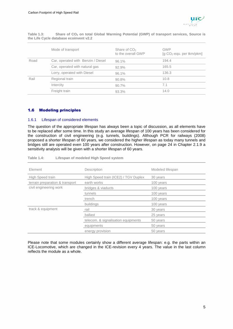
Table 1.3: Share of CO 2 on total Global Warming Potential (GWP) of transport services, Source is the Life Cycle database ecoinvent v2.2
Mode of transport Share of CO2
to the overall GWP GWP [g CO2-equ. per tkm/pkm]
Road Car, operated with Benzin / Diesel 96.1% 194.4
Car, operated with natural gas 92.9% 165.5
Lorry, operated with Diesel 96.1% 136.3
Rail Regional train 90.8% 10.8
Intercity 90.7% 7.1
Freight train 93.3% 14.0
1.6 Modeling principles
1.6.1 Lifespan of considered elements
The question of the appropriate lifespan has always been a topic of discussion, as all elements have to be replaced after some time. In this study an average lifespan of 100 years has been considered for the construction of civil engineering (e.g. tunnels, buildings). Although PCR for railways (2008) proposed a shorter lifespan of 60 years, we considered the higher lifespan as today many tunnels and bridges still are operated even 100 years after construction. However, on page 24 in Chapter 2.1.9 a sensitivity analysis will be given with a shorter lifespan of 60 years.
Table 1.4: Lifespan of modeled High Speed system
Element Description Modeled lifespan
High Speed train High Speed train (ICE2) / TGV Duplex 30 years
terrain preparation & transport earth works 100 years civil engineering work bridges & viaducts 100 years
tunnels 100 years
trench 100 years
buildings 100 years track & equipment rail 30 years
ballast 25 years
telecom. & signalisation equipments 50 years
equipments 50 years
energy provision 50 years
Please note that some modules certainly show a different average lifespan: e.g. the parts within an ICE-Locomotive, which are changed in the ICE-revision every 4 years. The value in the last column reflects the module as a whole.
6
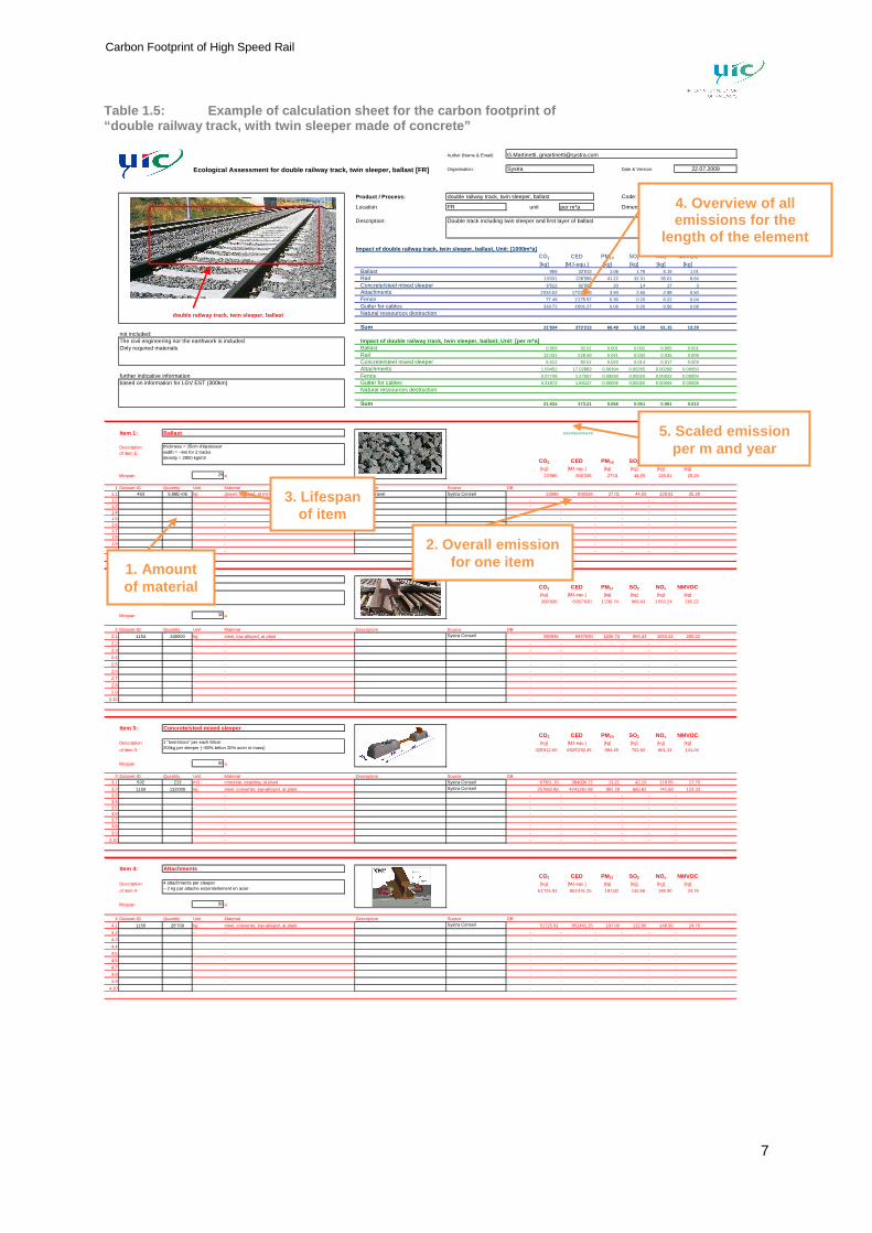
1.6.2 Modeling the components of High Speed line
To combine the different components of the construction of a high speed line (see Table 1.1), the following approach was used (see also von Rocycki et al. (2003)):
� The CO2 emissions from one item are calculated by multiplying the amount of material with the respective ecoinvent factors (see step 1 and step 2 below).
� The specific CO2 emissions per km are then calculated by dividing the overall emissions by the assumed lifespan of each element (see step 3 and step 4 below).
� The last step is to standardize the length to one km, e.g. from a bridge of 205m to 1 km of bridge (see step 5).
Example of calculation: Ballast from the track (see next page)
A track consists of steel rails on sleepers made from concrete, which are themselves laid on a bed of ballast. The track ballast is customarily crushed stone, in order to support the ties and allow some adjustment of their position. For a double track of 1,000m, around 2,600 m3 of crushed stone are needed. The production and transport of this ballast is linked with a carbon footprint of almost 24 metric ton CO2. As the ballast is replaced every 25 years, the annual carbon footprint per kilometer track can be calculated by a division of 25: 959 kg of CO2 are emitted from the ballast of 1km high speed track.
7
Carbon Footprint of High Speed Rail
Table 1.5: Example of calculation sheet for the carb on footprint of “double railway track, with twin sleeper made of co ncrete”
Author (Name & Email)
Organisation: Date & Version:
Product / Process: Code: 3.1
Location FR unit per m*a Dimension 1000 m
Description:
Impact of double railway track, twin sleeper, balla st, Unit: [1000m*a]CO2 CED PM10 SO2 NOx NMVOC[kg] [MJ-equ.] [kg] [kg] [kg] [kg]
Ballast 959 32'013 1.08 1.78 5.15 1.01
Rail 13'031 228'588 41.22 32.31 35.01 8.84
Concrete/steel mixed sleeper 6'512 92'506 20 14 17 3
Attachments 1'034.52 17'028.83 3.94 2.65 2.98 0.50
Fence 77.49 1'275.57 0.30 0.20 0.22 0.04
Gutter for cables 318.72 1'801.27 0.06 0.20 0.56 0.08
Natural ressources destruction
Sum 21'934 373'213 66.49 51.20 61.15 13.29
not included:Impact of double railway track, twin sleeper, balla st, Unit: [per m*a]Ballast 0.959 32.01 0.001 0.002 0.005 0.001
Rail 13.031 228.59 0.041 0.032 0.035 0.009
Concrete/steel mixed sleeper 6.512 92.51 0.020 0.014 0.017 0.003
Attachments 1.03452 17.02883 0.00394 0.00265 0.00298 0.00050
further indicative information Fence 0.07749 1.27557 0.00030 0.00020 0.00022 0.00004
Gutter for cables 0.31872 1.80127 0.00006 0.00020 0.00056 0.00008
Natural ressources destruction
Sum 21.934 373.21 0.066 0.051 0.061 0.013
Item 1: ############
Descriptionof item 1:
CO2 CED PM10 SO2 NOx NMVOC[kg] [MJ-equ.] [kg] [kg] [kg] [kg]
lifespan 25 a 23'986 800'336 27.01 44.55 128.81 25.28
1 Dataset-ID Quantity Unit Material Description Source DB1.1 463 5.88E+06 kg gravel, crushed, at mine crushed gravel Systra Conseil 23986 800336 27.01 44.55 128.81 25.281.2 - - - - - - - -1.3 - - - - - - - -1.4 - - - - - - - -1.5 - - - - - - - -1.6 - - - - - - - -1.7 - - - - - - - -1.8 - - - - - - - -
1.9 - - - - - - - -
1.10 - - - - - - - -
Item 2:CO2 CED PM10 SO2 NOx NMVOC
Description [kg] [MJ-equ.] [kg] [kg] [kg] [kg]
of item 2: 390'936 6'857'630 1'236.74 969.43 1'050.24 265.22
lifespan 30 a
2 Dataset-ID Quantity Unit Material Description Source DB
2.1 1154 240000 kg steel, low-alloyed, at plant Systra Conseil 390936 6857630 1236.74 969.43 1050.24 265.22
2.2 - - - - - - - -
2.3 - - - - - - - -
2.4 - - - - - - - -
2.5 - - - - - - - -
2.6 - - - - - - - -
2.7 - - - - - - - -
2.8 - - - - - - - -
2.9 - - - - - - - -
2.10 - - - - - - - -
Item 3:CO2 CED PM10 SO2 NOx NMVOC
Description [kg] [MJ-equ.] [kg] [kg] [kg] [kg]
of item 3: 325'612.00 4'625'292.45 994.49 702.92 861.24 141.04
lifespan 50 a
3 Dataset-ID Quantity Unit Material Description Source DB3.1 502 213 m3 concrete, exacting, at plant Systra Conseil 67951.10 384030.77 13.21 42.10 119.55 17.70
3.2 1150 133'000 kg steel, converter, low-alloyed, at plant Systra Conseil 257660.90 4241261.68 981.29 660.82 741.69 123.333.3 - - - - - - - -3.4 - - - - - - - -3.5 - - - - - - - -3.6 - - - - - - - -3.7 - - - - - - - -3.8 - - - - - - - -
3.9 - - - - - - - -
3.10 - - - - - - - -
Item 4:CO2 CED PM10 SO2 NOx NMVOC
Description [kg] [MJ-equ.] [kg] [kg] [kg] [kg]
of item 4: 51'725.91 851'441.25 197.00 132.66 148.90 24.76
lifespan 50 a
4 Dataset-ID Quantity Unit Material Description Source DB
4.1 1150 26'700 kg steel, converter, low-alloyed, at plant Systra Conseil 51725.91 851441.25 197.00 132.66 148.90 24.76
4.2 - - - - - - - -
4.3 - - - - - - - -
4.4 - - - - - - - -
4.5 - - - - - - - -
4.6 - - - - - - - -
4.7 - - - - - - - -
4.8 - - - - - - - -
4.9 - - - - - - - -
4.10 - - - - - - - -
G.Martinetti, [email protected]
22.07.2009Systra
Attachments
optional image4 attachments per sleeper~ 2 kg par attache essentiellement en acier
Ecological Assessment for double railway track, twi n sleeper, ballast [FR]
double railway track, twin sleeper, ballast
Double track including twin sleeper and first layer of ballast
based on information for LGV EST (300km)
The civil engineering nor the earthwork is included Only required materials
Concrete/steel mixed sleeper
1 "twin-blocs" per each 60cm200kg per sleeper (~80% béton 20% acier in mass) optional image
Ballast
Rail
60 kg/m 2 rails per track optional image
thickness = 35cm d'épaisseurwidth = ~6m for 2 tracksdensity = 2800 kg/m3
optional image
double railway track, twin sleeper, ballast
3. Lifespan of item
2. Overall emission for one item
4. Overview of all emissions for the
length of the element per year
5. Scaled emission per m and year
1. Amount of material
8
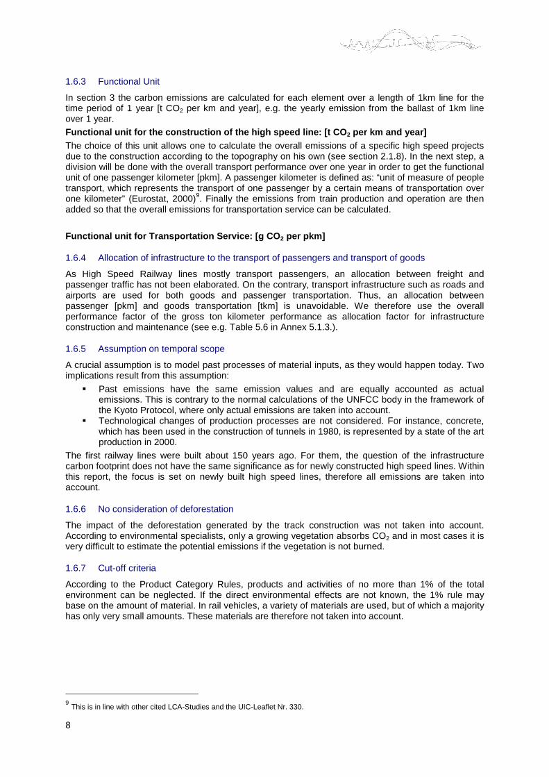
1.6.3 Functional Unit
In section 3 the carbon emissions are calculated for each element over a length of 1km line for the time period of 1 year [t CO2 per km and year], e.g. the yearly emission from the ballast of 1km line over 1 year.
Functional unit for the construction of the high sp eed line: [t CO 2 per km and year] The choice of this unit allows one to calculate the overall emissions of a specific high speed projects due to the construction according to the topography on his own (see section 2.1.8). In the next step, a division will be done with the overall transport performance over one year in order to get the functional unit of one passenger kilometer [pkm]. A passenger kilometer is defined as: “unit of measure of people transport, which represents the transport of one passenger by a certain means of transportation over one kilometer” (Eurostat, 2000)9. Finally the emissions from train production and operation are then added so that the overall emissions for transportation service can be calculated.
Functional unit for Transportation Service: [g CO 2 per pkm]
1.6.4 Allocation of infrastructure to the transport of passengers and transport of goods
As High Speed Railway lines mostly transport passengers, an allocation between freight and passenger traffic has not been elaborated. On the contrary, transport infrastructure such as roads and airports are used for both goods and passenger transportation. Thus, an allocation between passenger [pkm] and goods transportation [tkm] is unavoidable. We therefore use the overall performance factor of the gross ton kilometer performance as allocation factor for infrastructure construction and maintenance (see e.g. Table 5.6 in Annex 5.1.3.).
1.6.5 Assumption on temporal scope
A crucial assumption is to model past processes of material inputs, as they would happen today. Two implications result from this assumption:
� Past emissions have the same emission values and are equally accounted as actual emissions. This is contrary to the normal calculations of the UNFCC body in the framework of the Kyoto Protocol, where only actual emissions are taken into account.
� Technological changes of production processes are not considered. For instance, concrete, which has been used in the construction of tunnels in 1980, is represented by a state of the art production in 2000.
The first railway lines were built about 150 years ago. For them, the question of the infrastructure carbon footprint does not have the same significance as for newly constructed high speed lines. Within this report, the focus is set on newly built high speed lines, therefore all emissions are taken into account.
1.6.6 No consideration of deforestation
The impact of the deforestation generated by the track construction was not taken into account. According to environmental specialists, only a growing vegetation absorbs CO2 and in most cases it is very difficult to estimate the potential emissions if the vegetation is not burned.
1.6.7 Cut-off criteria
According to the Product Category Rules, products and activities of no more than 1% of the total environment can be neglected. If the direct environmental effects are not known, the 1% rule may base on the amount of material. In rail vehicles, a variety of materials are used, but of which a majority has only very small amounts. These materials are therefore not taken into account.
9 This is in line with other cited LCA-Studies and the UIC-Leaflet Nr. 330.
9
Carbon Footprint of High Speed Rail
2 Carbon footprint of high speed lines
2.1 Carbon footprint of the track construction
The construction is a step often forgotten in the carbon footprint calculation, because it is an occasional emission which occurs before the beginning of the operation of the line. According to the latest UIC Statistics (2011) a grand sum of 14,654 km of high speed lines operates worldwide. The lines differ in terms of topography or electricity mix, but in general all high speed lines consist of the following modules:
� Planning of the high speed line � Earthwork to build a track according to the needs (e.g. wide curves for high speed) � Track construction itself with ballast, rail and attachments (double track) � Civil engineering constructions as tunnels, viaducts and bridges � Equipment for energy transmission and telecommunication � Stations for passenger
In this chapter all carbon dioxide emissions from the above mentioned modules are separately analyzed. The overall carbon footprint of selected high speed rail lines will be elaborated in Chapter 2.2.2.
2.1.1 Emissions from planning phase
The conception stage of a high speed line project includes all the office works before the construction may start. The following assumptions have been made:
� It is assumed, that the final planning of 1km double track requires 50 workers over 1 year (The conception of the “LGV Mediterranée” lasted about 10 years).
� The electrical consumption per office desk is estimated with 1000 kWh per year (UCTE-electricity mix is assumed), the heating of the 1,500m2 office will be done by natural gas.
� About 10t of paper will be printed out for 1km of track
Carbon footprint: The result of the contribution of this step is 0.45 t CO2 by year for 1 km of line (double track). The most important part of the conception is the electricity for the computers and the central heating within the officej.
Conception phase
LGV Med ≈ 0.45 t CO2 /km/year
2.1.2 Emissions from earthworks
The carbon emissions from earthworks stems from:
� Excavation operations � Soil treatment � Backfill operations � Backfill material (cement / quicklime for soil improvement) � Platform materials production and transport
During the earthworks phase of the high speed line construction, considerable quantities of soil are moved and treated.
j Please note that transportation of people from the office (commuters or visits on site) is not taken into account here.
10
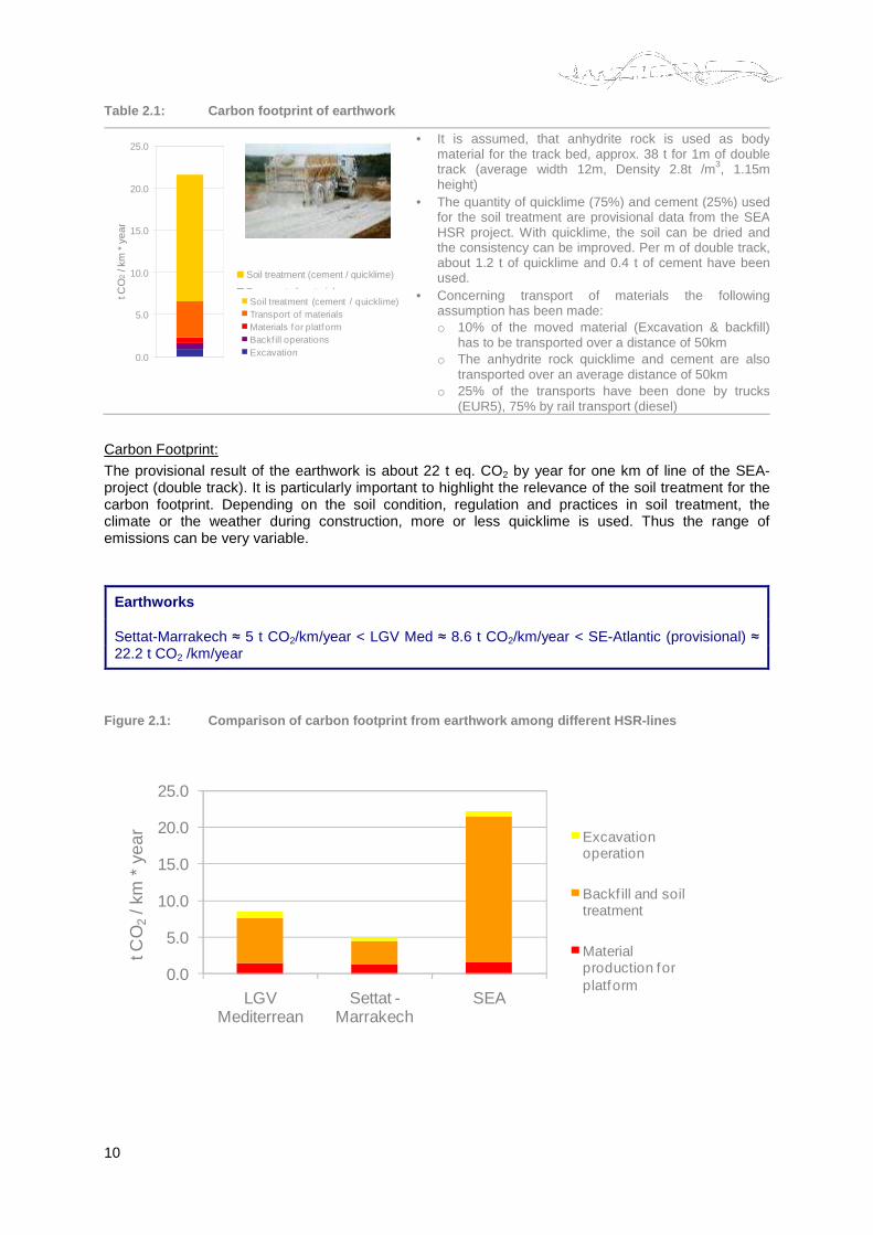
Table 2.1: Carbon footprint of earthwork
0.0
5.0
10.0
15.0
20.0
25.0
1
Soil treatment (cement / quicklime)
Transport of materials
Materials for platform
Backfill operations
Excavation
t CO
2 / k
m *
yea
r
• It is assumed, that anhydrite rock is used as body material for the track bed, approx. 38 t for 1m of double track (average width 12m, Density 2.8t /m3, 1.15m height)
• The quantity of quicklime (75%) and cement (25%) used for the soil treatment are provisional data from the SEA HSR project. With quicklime, the soil can be dried and the consistency can be improved. Per m of double track, about 1.2 t of quicklime and 0.4 t of cement have been used.
• Concerning transport of materials the following assumption has been made: o 10% of the moved material (Excavation & backfill)
has to be transported over a distance of 50km o The anhydrite rock quicklime and cement are also
transported over an average distance of 50km o 25% of the transports have been done by trucks
(EUR5), 75% by rail transport (diesel)
Carbon Footprint:
The provisional result of the earthwork is about 22 t eq. CO2 by year for one km of line of the SEA-project (double track). It is particularly important to highlight the relevance of the soil treatment for the carbon footprint. Depending on the soil condition, regulation and practices in soil treatment, the climate or the weather during construction, more or less quicklime is used. Thus the range of emissions can be very variable.
Earthworks
Settat-Marrakech ≈ 5 t CO2/km/year < LGV Med ≈ 8.6 t CO2/km/year < SE-Atlantic (provisional) ≈ 22.2 t CO2 /km/year
Figure 2.1: Comparison of carbon footprint from ear thwork among different HSR-lines
0.0
5.0
10.0
15.0
20.0
25.0
LGV Mediterrean
Settat -Marrakech
SEA
Excavation operation
Backf ill and soil treatment
Material production for platform
t CO
2/ k
m *
yea
r
Soil treatment (cement / quicklime)Transport of materialsMaterials for platformBackf ill operationsExcavation
11
Carbon Footprint of High Speed Rail
2.1.3 Emissions from the track construction (ballasted track and concrete slab track)
The emissions from the track construction include carbon emissions due to the production of materials required for the high speed line track:
� rail � ballast � sleepers � others (attachments, fence, gutter…)
There exist two main categories of high speed track: ballasted track and slab track. Most HSR lines have ballasted tracks; nevertheless some lines have a slab track (in Germany e.g. Köln-Frankfurt and Nürnberg-Ingolstadt, in Korea about 100km). All the necessary data were collected from specific literature. Please note that the maintenance of the track construction itself (as well as the other construction elements) is not considered in this carbon footprint, but somehow included in the reduced lifespan of certain elements (e.g. the rail will be replaced every 30 years, the ballast every 25 years).
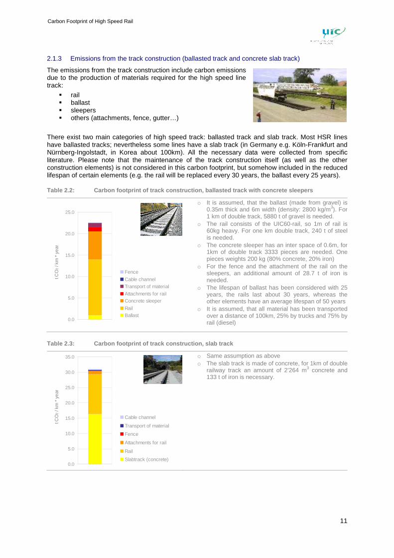
Table 2.2: Carbon footprint of track construction, ballasted track with concrete sleepers
0.0
5.0
10.0
15.0
20.0
25.0
1
Fence
Cable channelTransport of material
Attachments for railConcrete sleeper
RailBallast
t CO
2 / k
m *
yea
r
o It is assumed, that the ballast (made from gravel) is 0.35m thick and 6m width (density: 2800 kg/m3). For 1 km of double track, 5880 t of gravel is needed.
o The rail consists of the UIC60-rail, so 1m of rail is 60kg heavy. For one km double track, 240 t of steel is needed.
o The concrete sleeper has an inter space of 0.6m, for1km of double track 3333 pieces are needed. One pieces weights 200 kg (80% concrete, 20% iron)
o For the fence and the attachment of the rail on the sleepers, an additional amount of 28.7 t of iron is needed.
o The lifespan of ballast has been considered with 25 years, the rails last about 30 years, whereas the other elements have an average lifespan of 50 years
o It is assumed, that all material has been transported over a distance of 100km, 25% by trucks and 75% by rail (diesel)
Table 2.3: Carbon footprint of track construction, slab track
0.0
5.0
10.0
15.0
20.0
25.0
30.0
35.0
1
Cable channel
Transport of material
Fence
Attachments for rail
Rail
Slabtrack (concrete)
t CO
2 / k
m *
yea
r
o Same assumption as above o The slab track is made of concrete, for 1km of double
railway track an amount of 2’264 m3 concrete and 133 t of iron is necessary.
12
Carbon Footprint:
As the results show above, the emissions due to the construction are in both cases in the same order of magnitude (between 22.8 and 31.6 t eq. CO2 by km and year). The main emissions source for the track construction is the primary production of steel for the rail (about 50% of the total result).
Track construction (double track)
Ballasted Track (e.g. LGV Med) ≈ 22.8 t CO2 /km/year Concrete slab track (e.g. Taiwan, Germany…) ≈ 31.6 t CO2 /km/year
2.1.4 Emissions from civil engineering structures: Viaducts and Bridges
The carbon footprint of the civil engineering structures as viaducts over valleys and bridges has been elaborated as follows: On the one hand values from literature have been used (mainly from Schmied & Mottschall (2010). On the other hand data from projects about the required quantities of construction material have been collected by SYSTRA. All these quantities are then multiplied with the respective emission factor (see figure on the next page).
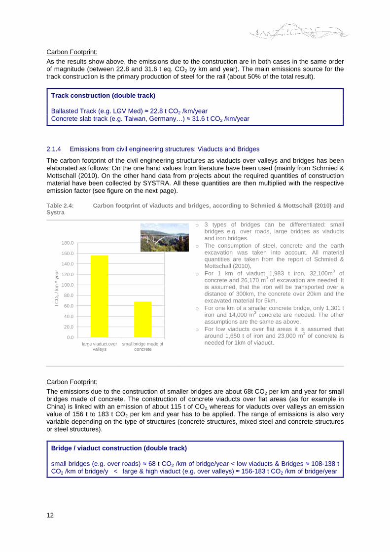
Table 2.4: Carbon footprint of viaducts and bridges , according to Schmied & Mottschall (2010) and Systra
0.0
20.0
40.0
60.0
80.0
100.0
120.0
140.0
160.0
180.0
large viaduct over valleys
small bridge made of concrete
t CO
2/ k
m *
yea
r
o 3 types of bridges can be differentiated: small bridges e.g. over roads, large bridges as viaducts and iron bridges.
o The consumption of steel, concrete and the earth excavation was taken into account. All material quantities are taken from the report of Schmied & Mottschall (2010),
o For 1 km of viaduct 1,983 t iron, 32,100m3 of concrete and 26,170 m3 of excavation are needed. It is assumed, that the iron will be transported over a distance of 300km, the concrete over 20km and the excavated material for 5km.
o For one km of a smaller concrete bridge, only 1,301 t iron and 14,000 m3 concrete are needed. The other assumptions are the same as above.
o For low viaducts over flat areas it is assumed that around 1,650 t of iron and 23,000 m3 of concrete is needed for 1km of viaduct.
Carbon Footprint:
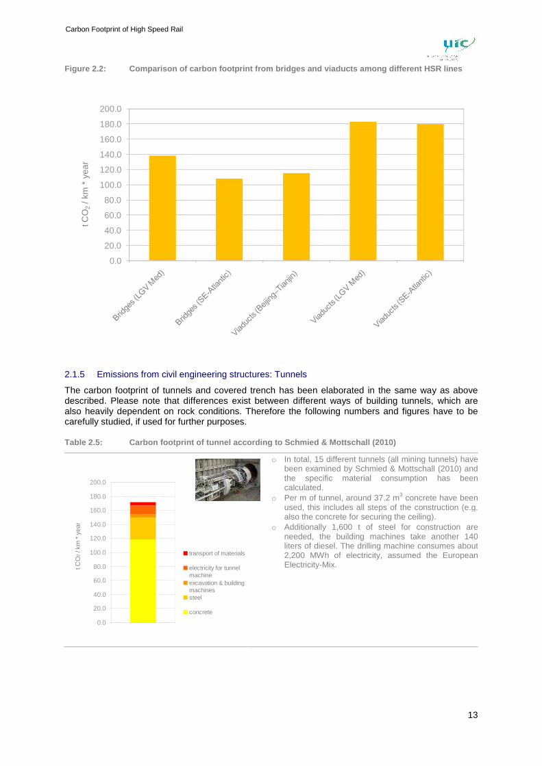
The emissions due to the construction of smaller bridges are about 68t CO2 per km and year for small bridges made of concrete. The construction of concrete viaducts over flat areas (as for example in China) is linked with an emission of about 115 t of CO2, whereas for viaducts over valleys an emission value of 156 t to 183 t CO2 per km and year has to be applied. The range of emissions is also very variable depending on the type of structures (concrete structures, mixed steel and concrete structures or steel structures).
Bridge / viaduct construction (double track)
small bridges (e.g. over roads) ≈ 68 t CO2 /km of bridge/year < low viaducts & Bridges ≈ 108-138 t CO2 /km of bridge/y < large & high viaduct (e.g. over valleys) ≈ 156-183 t CO2 /km of bridge/year
13
Carbon Footprint of High Speed Rail
Figure 2.2: Comparison of carbon footprint from bri dges and viaducts among different HSR lines
0.0
20.0
40.0
60.0
80.0
100.0
120.0
140.0
160.0
180.0
200.0
t CO
2/ k
m *
yea
r
2.1.5 Emissions from civil engineering structures: Tunnels
The carbon footprint of tunnels and covered trench has been elaborated in the same way as above described. Please note that differences exist between different ways of building tunnels, which are also heavily dependent on rock conditions. Therefore the following numbers and figures have to be carefully studied, if used for further purposes.
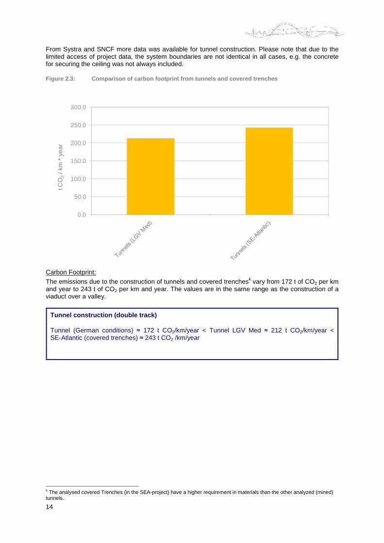
Table 2.5: Carbon footprint of tunnel according to Schmied & Mottschall (2010)
0.0
20.0
40.0
60.0
80.0
100.0
120.0
140.0
160.0
180.0
200.0
1
transport of materials
electricity for tunnelmachineexcavation & buildingmachinessteel
concrete
t CO
2 / k
m *
yea
r
o In total, 15 different tunnels (all mining tunnels) havebeen examined by Schmied & Mottschall (2010) and the specific material consumption has been calculated.
o Per m of tunnel, around 37.2 m3 concrete have been used, this includes all steps of the construction (e.g. also the concrete for securing the ceiling).
o Additionally 1,600 t of steel for construction are needed, the building machines take another 140 liters of diesel. The drilling machine consumes about 2,200 MWh of electricity, assumed the European Electricity-Mix.
14
From Systra and SNCF more data was available for tunnel construction. Please note that due to the limited access of project data, the system boundaries are not identical in all cases, e.g. the concrete for securing the ceiling was not always included.
Figure 2.3: Comparison of carbon footprint from tun nels and covered trenches
0.0
50.0
100.0
150.0
200.0
250.0
300.0
t CO
2/ k
m *
yea
r
Carbon Footprint:
The emissions due to the construction of tunnels and covered trenchesk vary from 172 t of CO2 per km and year to 243 t of CO2 per km and year. The values are in the same range as the construction of a viaduct over a valley.
Tunnel construction (double track)
Tunnel (German conditions) ≈ 172 t CO2/km/year < Tunnel LGV Med ≈ 212 t CO2/km/year < SE-Atlantic (covered trenches) ≈ 243 t CO2 /km/year
k The analysed covered Trenches (in the SEA-project) have a higher requirement in materials than the other analyzed (mined) tunnels.
15
Carbon Footprint of High Speed Rail
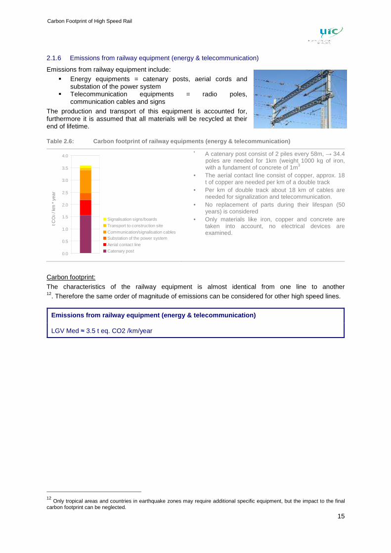
2.1.6 Emissions from railway equipment (energy & telecommunication)
Emissions from railway equipment include:
� Energy equipments = catenary posts, aerial cords and substation of the power system
� Telecommunication equipments = radio poles, communication cables and signs
The production and transport of this equipment is accounted for, furthermore it is assumed that all materials will be recycled at their end of lifetime.
Table 2.6: Carbon footprint of railway equipments ( energy & telecommunication)
0.0
0.5
1.0
1.5
2.0
2.5
3.0
3.5
4.0
1
Signalisation signs/boards
Transport to construction site
Communication/signalisation cablesSubstation of the power system
Aerial contact line
Catenary post
t CO
2 / k
m *
yea
r
• A catenary post consist of 2 piles every 58m, → 34.4 poles are needed for 1km (weight 1000 kg of iron, with a fundament of concrete of 1m3
• The aerial contact line consist of copper, approx. 18 t of copper are needed per km of a double track
• Per km of double track about 18 km of cables are needed for signalization and telecommunication.
• No replacement of parts during their lifespan (50years) is considered
• Only materials like iron, copper and concrete are taken into account, no electrical devices are examined.
Carbon footprint:
The characteristics of the railway equipment is almost identical from one line to another12. Therefore the same order of magnitude of emissions can be considered for other high speed lines.
Emissions from railway equipment (energy & telecomm unication)
LGV Med ≈ 3.5 t eq. CO2 /km/year
12 Only tropical areas and countries in earthquake zones may require additional specific equipment, but the impact to the final carbon footprint can be neglected.
16
2.1.7 Emissions from station and technical centers (only construction)
Two kinds of stations were considered: a main station and a secondary station (e.g. Valence as a main station, and Aix-en-Provence TGV station as a secondary station). The construction of both stations was estimated according to existing data of Germany (Schmied & Mottschall 2010)
Please note that the number of stations by km along a line may be very different. Therefore the functional unit of this particular element is t CO 2 per unit and year (instead of t CO2 per km and year).
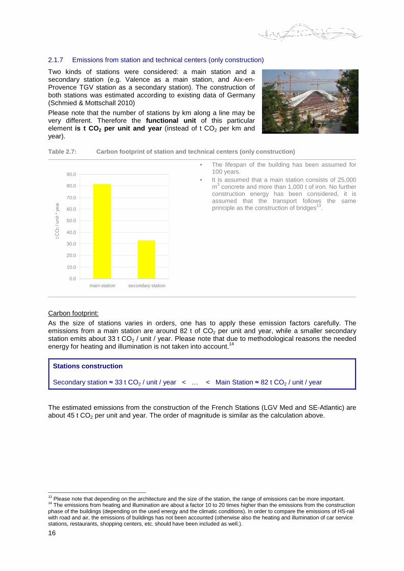
Table 2.7: Carbon footprint of station and technica l centers (only construction)
0.0
10.0
20.0
30.0
40.0
50.0
60.0
70.0
80.0
90.0
main station secondary station
t CO
2 / u
nit *
yea
r
• The lifespan of the building has been assumed for 100 years.
• It is assumed that a main station consists of 25,000 m3 concrete and more than 1,000 t of iron. No further construction energy has been considered, it is assumed that the transport follows the same principle as the construction of bridges13.
Carbon footprint:
As the size of stations varies in orders, one has to apply these emission factors carefully. The emissions from a main station are around 82 t of CO2 per unit and year, while a smaller secondary station emits about 33 t CO2 / unit / year. Please note that due to methodological reasons the needed energy for heating and illumination is not taken into account.14
Stations construction
Secondary station ≈ 33 t CO2 / unit / year < … < Main Station ≈ 82 t CO2 / unit / year
The estimated emissions from the construction of the French Stations (LGV Med and SE-Atlantic) are about 45 t CO2 per unit and year. The order of magnitude is similar as the calculation above.
13 Please note that depending on the architecture and the size of the station, the range of emissions can be more important. 14 The emissions from heating and illumination are about a factor 10 to 20 times higher than the emissions from the construction phase of the buildings (depending on the used energy and the climatic conditions). In order to compare the emissions of HS-rail with road and air, the emissions of buildings has not been accounted (otherwise also the heating and illumination of car service stations, restaurants, shopping centers, etc. should have been included as well.).
17
Carbon Footprint of High Speed Rail
2.1.8 Carbon footprint of the construction of selected High Speed lines
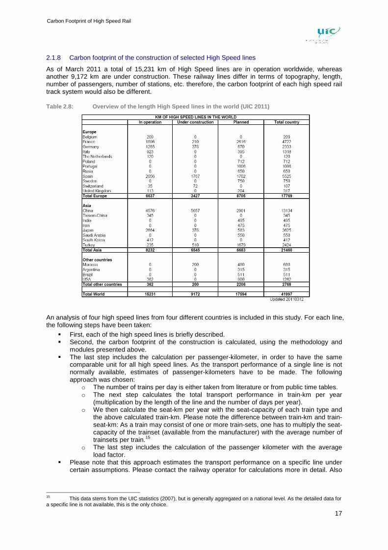
As of March 2011 a total of 15,231 km of High Speed lines are in operation worldwide, whereas another 9,172 km are under construction. These railway lines differ in terms of topography, length, number of passengers, number of stations, etc. therefore, the carbon footprint of each high speed rail track system would also be different.
Table 2.8: Overview of the length High Speed lines i n the world (UIC 2011)
An analysis of four high speed lines from four different countries is included in this study. For each line, the following steps have been taken:
� First, each of the high speed lines is briefly described. � Second, the carbon footprint of the construction is calculated, using the methodology and
modules presented above. � The last step includes the calculation per passenger-kilometer, in order to have the same
comparable unit for all high speed lines. As the transport performance of a single line is not normally available, estimates of passenger-kilometers have to be made. The following approach was chosen:
o The number of trains per day is either taken from literature or from public time tables. o The next step calculates the total transport performance in train-km per year
(multiplication by the length of the line and the number of days per year). o We then calculate the seat-km per year with the seat-capacity of each train type and
the above calculated train-km. Please note the difference between train-km and train-seat-km: As a train may consist of one or more train-sets, one has to multiply the seat-capacity of the trainset (available from the manufacturer) with the average number of trainsets per train.15
o The last step includes the calculation of the passenger kilometer with the average load factor.
� Please note that this approach estimates the transport performance on a specific line under certain assumptions. Please contact the railway operator for calculations more in detail. Also
15 This data stems from the UIC statistics (2007), but is generally aggregated on a national level. As the detailed data for a specific line is not available, this is the only choice.
18
note that the emission from rolling stock and operation are not yet integrated (see chapter 2.2.1 and 2.2.2).
19
Carbon Footprint of High Speed Rail
LGV Mediterranée High Speed line
1. Description
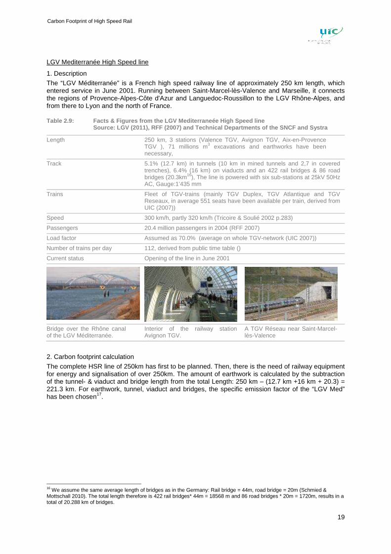
The “LGV Méditerranée” is a French high speed railway line of approximately 250 km length, which entered service in June 2001. Running between Saint-Marcel-lès-Valence and Marseille, it connects the regions of Provence-Alpes-Côte d'Azur and Languedoc-Roussillon to the LGV Rhône-Alpes, and from there to Lyon and the north of France.
Table 2.9: Facts & Figures from the LGV Mediterraneé e High Speed line Source: LGV (2011), RFF (2007) and Technical Departme nts of the SNCF and Systra
Length 250 km, 3 stations (Valence TGV, Avignon TGV, Aix-en-Provence TGV ), 71 millions m3 excavations and earthworks have been necessary,
Track 5.1% (12.7 km) in tunnels (10 km in mined tunnels and 2,7 in covered trenches), 6.4% (16 km) on viaducts and an 422 rail bridges & 86 road bridges (20.3km16), The line is powered with six sub-stations at 25kV 50Hz AC, Gauge:1’435 mm
Trains Fleet of TGV-trains (mainly TGV Duplex, TGV Atlantique and TGV Reseaux, in average 551 seats have been available per train, derived from UIC (2007))
Speed 300 km/h, partly 320 km/h (Tricoire & Soulié 2002 p.283)
Passengers 20.4 million passengers in 2004 (RFF 2007)
Load factor Assumed as 70.0% (average on whole TGV-network (UIC 2007))
Number of trains per day 112, derived from public time table ()
Current status Opening of the line in June 2001
Bridge over the Rhône canal of the LGV Méditerranée.
Interior of the railway station Avignon TGV.
A TGV Réseau near Saint-Marcel-lès-Valence
2. Carbon footprint calculation
The complete HSR line of 250km has first to be planned. Then, there is the need of railway equipment for energy and signalisation of over 250km. The amount of earthwork is calculated by the subtraction of the tunnel- & viaduct and bridge length from the total Length: 250 km – (12.7 km +16 km + 20.3) = 221.3 km. For earthwork, tunnel, viaduct and bridges, the specific emission factor of the “LGV Med” has been chosen17.
16 We assume the same average length of bridges as in the Germany: Rail bridge = 44m, road bridge = 20m (Schmied & Mottschall 2010). The total length therefore is 422 rail bridges* 44m = 18568 m and 86 road bridges * 20m = 1720m, results in a total of 20.288 km of bridges.
20
Table 2.10: Carbon Footprint “LGV Mediterranée High Speed line”
Quantity Carbon Footprint of construction
Conception 0.45 t CO2 per km and year 250 km 112.5 t CO2 per year
Railway equipment 3.5 t CO2 per km and year 250 km 875 t CO2 per year
Rail 22.8 t CO2 per km and year 250 km 5700 t CO2 per year
Tunnel 212.5 t CO2 per km and year 12.7 km 2698.8 t CO2 per year
Viaduct 183 t CO2 per km and year 16 km 2928 t CO2 per year
Bridges 139 t CO2 per km and year 20.3 km 2821.7 t CO2 per year
Earthwork 8.57 t CO2 per km and year 201 km 1722.57 t CO2 per year
Main Station 82 t CO2 per unit and year 2 stations 164 t CO2 per year
Secondary Station 33 t CO2 unit and year 1 station 33 t CO2 per year
Total - - 17,055.5 t CO2 per year
3. Calculation of CO2 per passenger kilometre
As noted above, it is necessary to estimate the transport performance: 112 trains are running everyday between Valence and Marseille, which results in a total of 10.22 Million train-kilometres per year. Multiplied with the number of available seats per train (551 seats, derived from UIC (2007)) and the average load factor of the TGV-lines of 70%, UIC (2007), we may estimate the total transport performance as 3,939,000,000 pkm. We divide now the total carbon dioxide emissions from the construction phase through the performance in pkm, in order to get the average carbon footprint per passenger and pkm.
The carbon footprint per passenger is therefore about 4.3g CO 2 per pkm for the construction of the high speed line “LGV Mediterranean”.
South Europe Atlantic (SEA) High Speed line
1. Description
The South Europe Atlantic (SEA) project represents the extension of the Atlantic HSL currently linking Paris and Tours further to the South. The high-speed line connects Tours and Bordeaux and is 340km long.
Table 2.11: Facts & Figures from the South Europe At lantic (SEA) High Speed line (RFF 2011)
Length 302 km, no station, but 40 extra km of connecting line to existing stations (not considered)
Track 404 bridges18 (3.1% of the length, resp. 9.3km) and 19 viaducts (3.3% of the length, resp. 10 km), 7 covered trenches (1km)19, 38 km of noise walls and 26 km of noise screens, 25kV 50Hz AC catenary, Gauge:1,435 mm, 46 million m3 of excavations and 30 million m3 of earthworks
Trains Fleet of TGV-trains, we assume an average of 551 seats per train as for LGV Med
Speed 320 km/h
Passengers 19-20 million passengers per year are expected (Forecast from RFF (2011))
Load factor We assume the similar load factor of 70% as derived from UIC (2007)
Current status Preliminary studies started in 1997, construction should start in 2011, trains are expected to run in 2016
18 As the overall length of the bridges is not available, the number of bridges has been multiplied with the average length of rail- and roadbridges (23m) in Germany ((Schmied & Mottschall 2010): 404 bridges * 23m = 9.292 km 19 The length of covered trenches was only available for a subsection. Based on the whole line, the overall length was extrapolated as an estimation of 1km.
21
Carbon Footprint of High Speed Rail
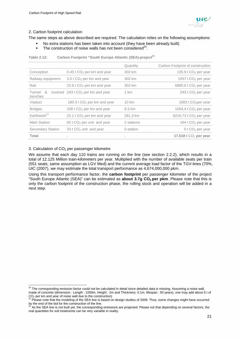
2. Carbon footprint calculation
The same steps as above described are required. The calculation relies on the following assumptions:
� No extra stations has been taken into account (they have been already built) � The construction of noise walls has not been considered20.
Table 2.12: Carbon Footprint “South Europe Atlantic ( SEA)-project 21
Quantity Carbon Footprint of construction
Conception 0.45 t CO2 per km and year 302 km 135.9 t CO2 per year
Railway equipment 3.5 t CO2 per km and year 302 km 1057 t CO2 per year
Rail 22.8 t CO2 per km and year 302 km 6885.6 t CO2 per year
Tunnel & covered trenches
243 t CO2 per km and year 1 km 243 t CO2 per year
Viaduct 180.3 t CO2 per km and year 10 km 1803 t CO2per year
Bridges 108 t CO2 per km and year 9.3 km 1004,4 t CO2 per year
Earthwork22 22.1 t CO2 per km and year 281.3 km 6216.73 t CO2 per year
Main Station 82 t CO2 per unit and year 2 stations 164 t CO2 per year
Secondary Station 33 t CO2 unit and year 0 station 0 t CO2 per year
Total - - 17,518 t CO2 per year
3. Calculation of CO2 per passenger kilometre
We assume that each day 110 trains are running on the line (see section 2.2.2), which results in a total of 12.125 Million train-kilometers per year. Multiplied with the number of available seats per train (551 seats, same assumption as LGV Med) and the current average load factor of the TGV-lines (70%, UIC (2007), we may estimate the total transport performance as 4,674,000,000 pkm.
Using this transport performance factor, the carbon footprint per passenger kilometer of the project “South Europe Atlantic (SEA)” can be estimated as about 3.7g CO 2 per pkm . Please note that this is only the carbon footprint of the construction phase, the rolling stock and operation will be added in a next step.
20 The corresponding emission factor could not be calculated in detail since detailed data is missing. Assuming a noise wall, made of concrete (dimension : Length : 1000m, Height : 2m and Thickness: 0.1m, lifespan : 50 years), one may add about 6 t of CO2 per km and year of noise wall due to the construction) 21 Please note that the modeling of the SEA line is based on design studies of 2009. Thus, some changes might have occurred by the end of the bid for the construction of the line. 22 As the SEA line is not built yet, the corresponding emissions are projected. Please not that depending on several factors, the real quantities for soil treatments can be very variable in reality.
22
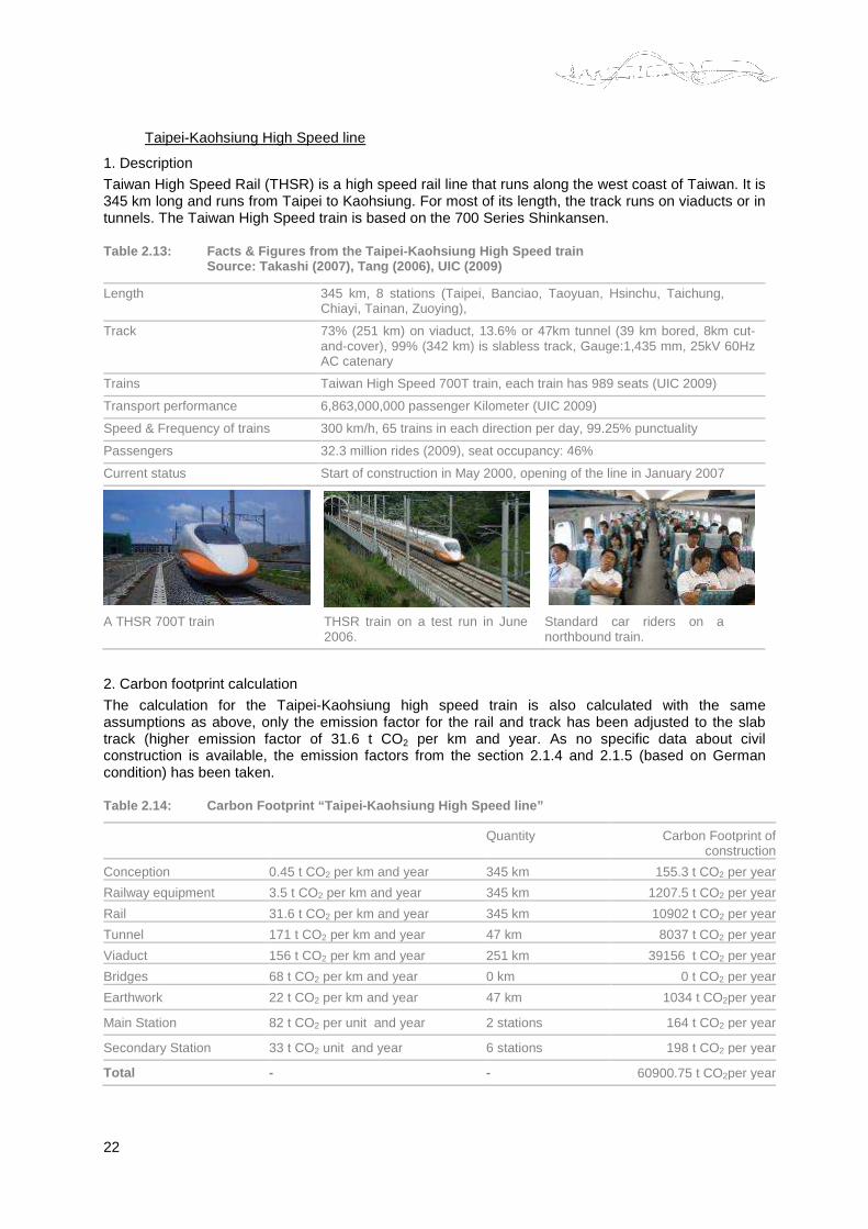
Taipei-Kaohsiung High Speed line
1. Description
Taiwan High Speed Rail (THSR) is a high speed rail line that runs along the west coast of Taiwan. It is 345 km long and runs from Taipei to Kaohsiung. For most of its length, the track runs on viaducts or in tunnels. The Taiwan High Speed train is based on the 700 Series Shinkansen.
Table 2.13: Facts & Figures from the Taipei-Kaohsiu ng High Speed train Source: Takashi (2007), Tang (2006), UIC (2009)
Length 345 km, 8 stations (Taipei, Banciao, Taoyuan, Hsinchu, Taichung, Chiayi, Tainan, Zuoying),
Track 73% (251 km) on viaduct, 13.6% or 47km tunnel (39 km bored, 8km cut-and-cover), 99% (342 km) is slabless track, Gauge:1,435 mm, 25kV 60Hz AC catenary
Trains Taiwan High Speed 700T train, each train has 989 seats (UIC 2009)
Transport performance 6,863,000,000 passenger Kilometer (UIC 2009)
Speed & Frequency of trains 300 km/h, 65 trains in each direction per day, 99.25% punctuality
Passengers 32.3 million rides (2009), seat occupancy: 46%
Current status Start of construction in May 2000, opening of the line in January 2007
A THSR 700T train THSR train on a test run in June 2006.
Standard car riders on a northbound train.
2. Carbon footprint calculation
The calculation for the Taipei-Kaohsiung high speed train is also calculated with the same assumptions as above, only the emission factor for the rail and track has been adjusted to the slab track (higher emission factor of 31.6 t CO2 per km and year. As no specific data about civil construction is available, the emission factors from the section 2.1.4 and 2.1.5 (based on German condition) has been taken.
Table 2.14: Carbon Footprint “Taipei-Kaohsiung High Speed line”
Quantity Carbon Footprint of construction
Conception 0.45 t CO2 per km and year 345 km 155.3 t CO2 per year
Railway equipment 3.5 t CO2 per km and year 345 km 1207.5 t CO2 per year
Rail 31.6 t CO2 per km and year 345 km 10902 t CO2 per year
Tunnel 171 t CO2 per km and year 47 km 8037 t CO2 per year
Viaduct 156 t CO2 per km and year 251 km 39156 t CO2 per year
Bridges 68 t CO2 per km and year 0 km 0 t CO2 per year
Earthwork 22 t CO2 per km and year 47 km 1034 t CO2per year
Main Station 82 t CO2 per unit and year 2 stations 164 t CO2 per year
Secondary Station 33 t CO2 unit and year 6 stations 198 t CO2 per year
Total - - 60900.75 t CO2per year
23
Carbon Footprint of High Speed Rail
3. Calculation of CO2 per passenger kilometre
According to the actual UIC statistics (2009), the Taiwan High Speed Rail has a yearly transport performance of 6,863,000,000 passenger Kilometer (see Chapter 2.2.1 and 2.2.2 for detailed calculations). The carbon footprint per passenger due to the infrastructure is therefore about 8.9g CO2 per pkm for the HS-line “Taipei-Kaohsiung”. Please note, that the emission from rolling stock and operation are not yet integrated.
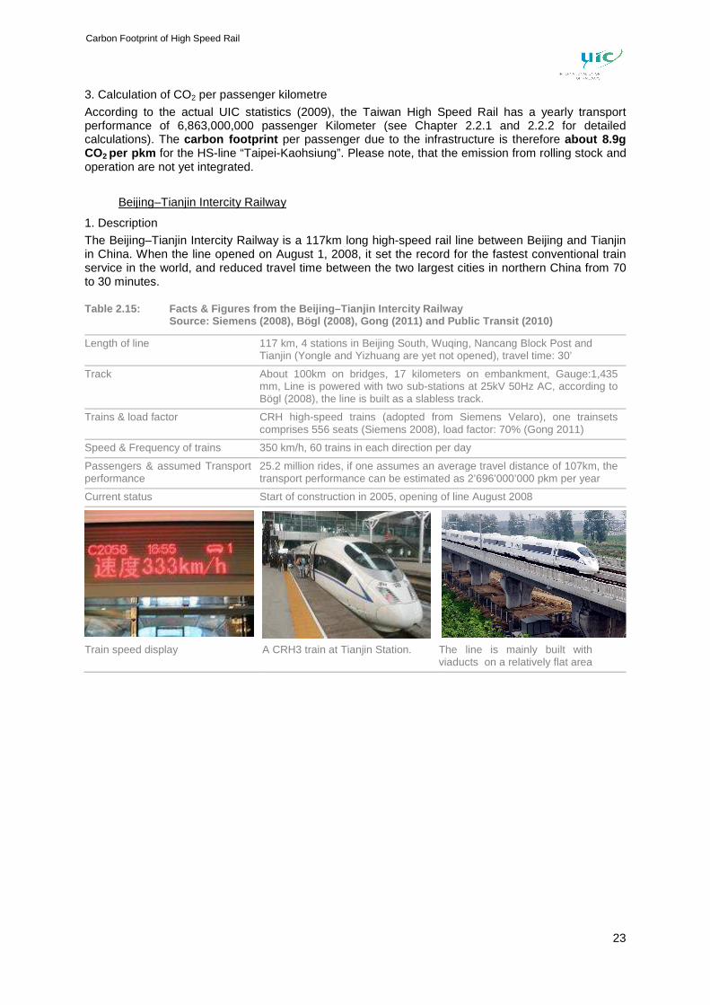
Beijing–Tianjin Intercity Railway
1. Description
The Beijing–Tianjin Intercity Railway is a 117km long high-speed rail line between Beijing and Tianjin in China. When the line opened on August 1, 2008, it set the record for the fastest conventional train service in the world, and reduced travel time between the two largest cities in northern China from 70 to 30 minutes.
Table 2.15: Facts & Figures from the Beijing–Tianji n Intercity Railway Source: Siemens (2008), Bögl (2008), Gong (2011) and Public Transit (2010)
Length of line 117 km, 4 stations in Beijing South, Wuqing, Nancang Block Post and Tianjin (Yongle and Yizhuang are yet not opened), travel time: 30’
Track About 100km on bridges, 17 kilometers on embankment, Gauge:1,435 mm, Line is powered with two sub-stations at 25kV 50Hz AC, according to Bögl (2008), the line is built as a slabless track.
Trains & load factor CRH high-speed trains (adopted from Siemens Velaro), one trainsets comprises 556 seats (Siemens 2008), load factor: 70% (Gong 2011)
Speed & Frequency of trains 350 km/h, 60 trains in each direction per day
Passengers & assumed Transport performance
25.2 million rides, if one assumes an average travel distance of 107km, the transport performance can be estimated as 2’696’000’000 pkm per year
Current status Start of construction in 2005, opening of line August 2008
Train speed display A CRH3 train at Tianjin Station. The line is mainly built with
viaducts on a relatively flat area
24
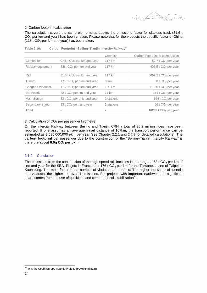
2. Carbon footprint calculation
The calculation covers the same elements as above, the emissions factor for slabless track (31.6 t CO2 per km and year) has been chosen. Please note that for the viaducts the specific factor of China (115 t CO2 per km and year) has been taken.
Table 2.16: Carbon Footprint “Beijing–Tianjin Inter city Railway”
Quantity Carbon Footprint of construction
Conception 0.45 t CO2 per km and year 117 km 52.7 t CO2 per year
Railway equipment 3.5 t CO2 per km and year 117 km 409.5 t CO2 per year
Rail 31.6 t CO2 per km and year 117 km 3697.2 t CO2 per year
Tunnel 171 t CO2 per km and year 0 km 0 t CO2 per year
Bridges / Viaducts 115 t CO2 per km and year 100 km 11500 t CO2 per year
Earthwork 22 t CO2 per km and year 17 km 374 t CO2 per year
Main Station 82 t CO2 per unit and year 2 stations 164 t CO2per year
Secondary Station 33 t CO2 unit and year 2 stations 66 t CO2 per year
Total - - 16263 t CO2 per year
3. Calculation of CO2 per passenger kilometre
On the Intercity Railway between Beijing and Tianjin CRH a total of 25.2 million rides have been reported. If one assumes an average travel distance of 107km, the transport performance can be estimated as 2,696,000,000 pkm per year (see Chapter 2.2.1 and 2.2.2 for detailed calculations). The carbon footprint per passenger due to the construction of the “Beijing–Tianjin Intercity Railway” is therefore about 6.0g CO 2 per pkm .
2.1.9 Conclusion
The emissions from the construction of the high speed rail lines lies in the range of 58 t CO2 per km of line and year for the SEA- Project in France and 176 t CO2 per km for the Taiwanese Line of Taipei to Kaohsiung. The main factor is the number of viaducts and tunnels: The higher the share of tunnels and viaducts, the higher the overall emissions. For projects with important earthworks, a significant share comes from the use of quicklime and cement for soil stabilization23.
23 e.g. the South Europe Atlantic Project (provisional data)
25
Carbon Footprint of High Speed Rail
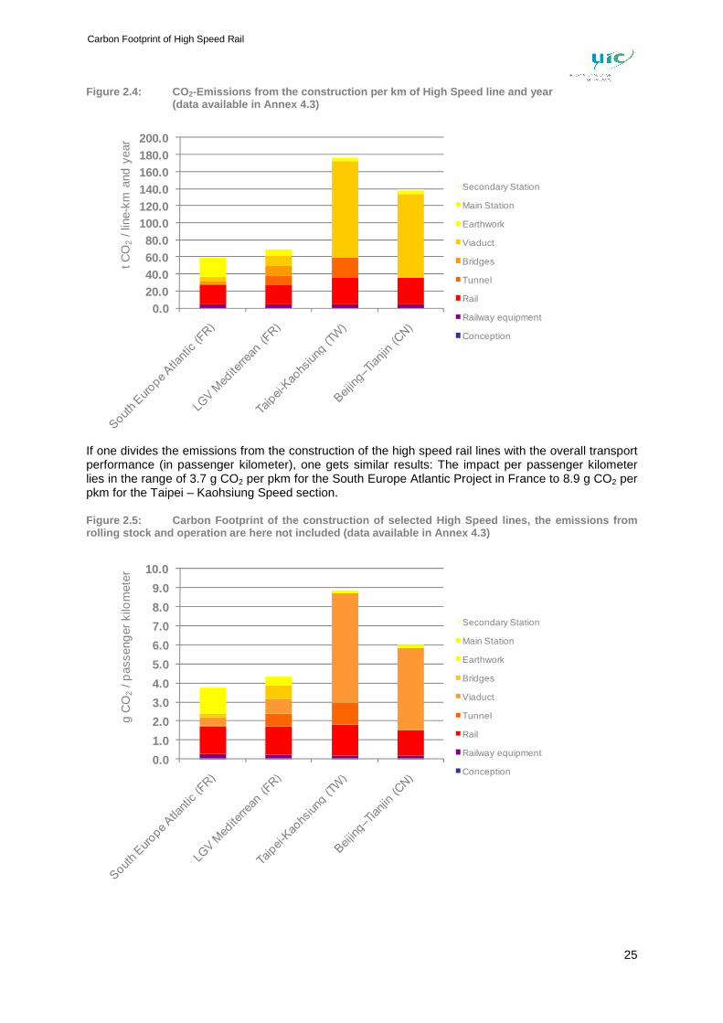
Figure 2.4: CO 2-Emissions from the construction per km of High Spee d line and year (data available in Annex 4.3)
0.020.040.060.080.0
100.0120.0140.0160.0180.0200.0
Secondary Station
Main Station
Earthwork
Viaduct
Bridges
Tunnel
Rail
Railway equipment
Conception
t CO
2/ l
ine-
km a
nd y
ear
If one divides the emissions from the construction of the high speed rail lines with the overall transport performance (in passenger kilometer), one gets similar results: The impact per passenger kilometer lies in the range of 3.7 g CO2 per pkm for the South Europe Atlantic Project in France to 8.9 g CO2 per pkm for the Taipei – Kaohsiung Speed section.
Figure 2.5: Carbon Footprint of the construction of selected High Speed lines, the emissions from rolling stock and operation are here not included ( data available in Annex 4.3)
0.0
1.0
2.0
3.0
4.0
5.0
6.0
7.0
8.0
9.0
10.0
Secondary Station
Main Station
Earthwork
Bridges
Viaduct
Tunnel
Rail
Railway equipment
Conception
g C
O2
/ pas
seng
er k
ilom
eter
26
One may conclude that differences between different high speed lines exist, but the emissions are all lying in the same order of size. Please note that the mostly more important emissions from operation and rolling stock are yet not included (see section 2.3).
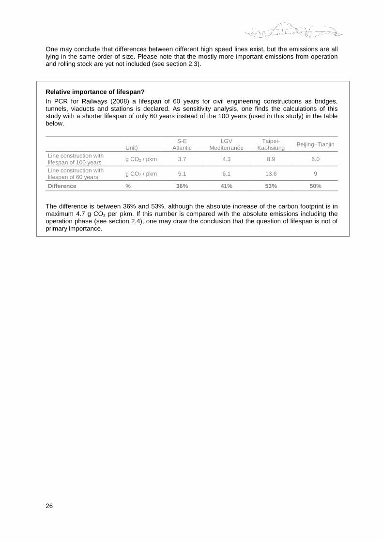
Relative importance of lifespan? In PCR for Railways (2008) a lifespan of 60 years for civil engineering constructions as bridges, tunnels, viaducts and stations is declared. As sensitivity analysis, one finds the calculations of this study with a shorter lifespan of only 60 years instead of the 100 years (used in this study) in the table below.
Unit) S-E
Atlantic LGV
Mediterranée Taipei-
Kaohsiung Beijing–Tianjin
Line construction with lifespan of 100 years g CO2 / pkm 3.7 4.3 8.9 6.0
Line construction with lifespan of 60 years g CO2 / pkm 5.1 6.1 13.6 9
Difference % 36% 41% 53% 50%
The difference is between 36% and 53%, although the absolute increase of the carbon footprint is in maximum 4.7 g CO2 per pkm. If this number is compared with the absolute emissions including the operation phase (see section 2.4), one may draw the conclusion that the question of lifespan is not of primary importance.
27
Carbon Footprint of High Speed Rail
2.2 Carbon Footprint of High Speed rolling stock
2.2.1 Emissions from construction, maintenance and disposal of rolling stock
Precise data has been obtained for the German high speed train ICE2. From other trains as e.g. the French “TGV duplex” only rough materials composition has been collected.
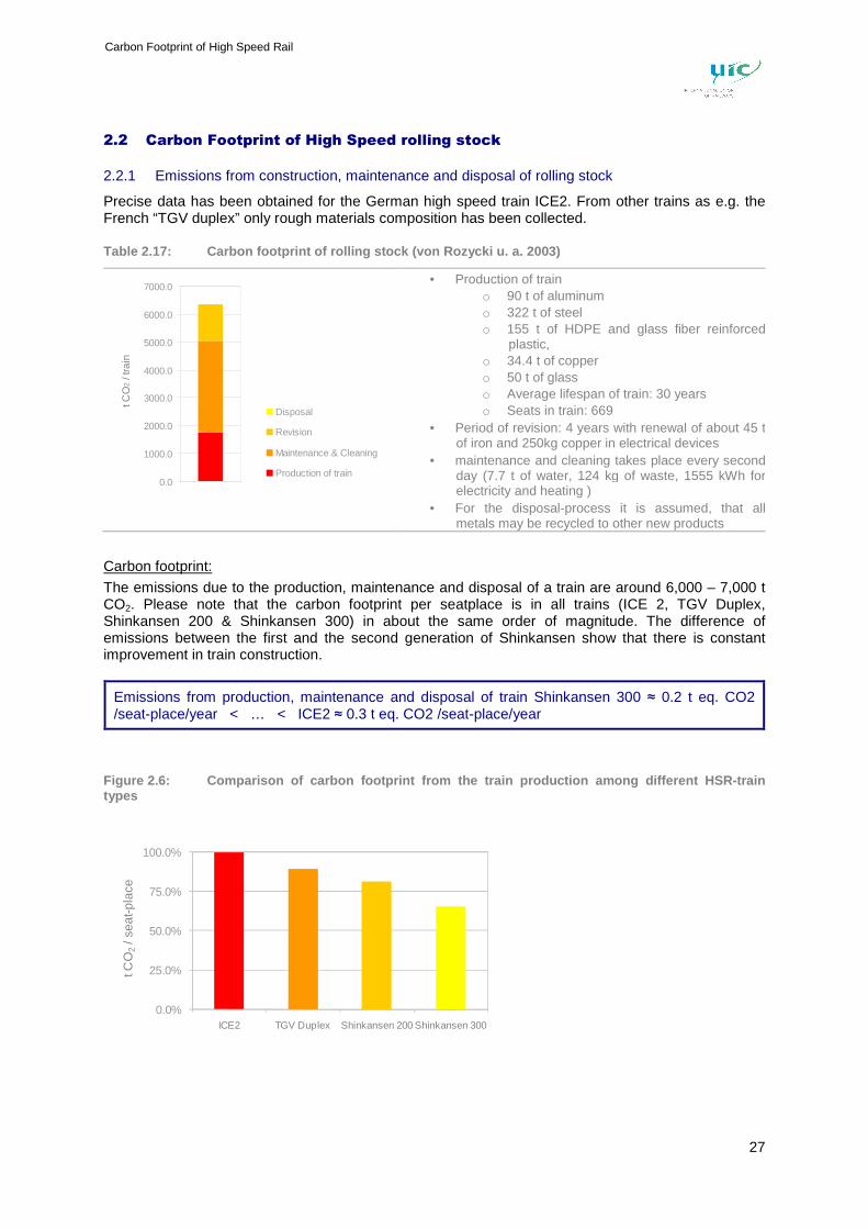
Table 2.17: Carbon footprint of rolling stock (von Rozycki u. a. 2003)
0.0
1000.0
2000.0
3000.0
4000.0
5000.0
6000.0
7000.0
1
Disposal
Revision
Maintenance & Cleaning
Production of train
t CO
2 / t
rain
• Production of train o 90 t of aluminum o 322 t of steel o 155 t of HDPE and glass fiber reinforced
plastic, o 34.4 t of copper o 50 t of glass o Average lifespan of train: 30 years o Seats in train: 669
• Period of revision: 4 years with renewal of about 45 t of iron and 250kg copper in electrical devices
• maintenance and cleaning takes place every second day (7.7 t of water, 124 kg of waste, 1555 kWh for electricity and heating )
• For the disposal-process it is assumed, that all metals may be recycled to other new products
Carbon footprint:
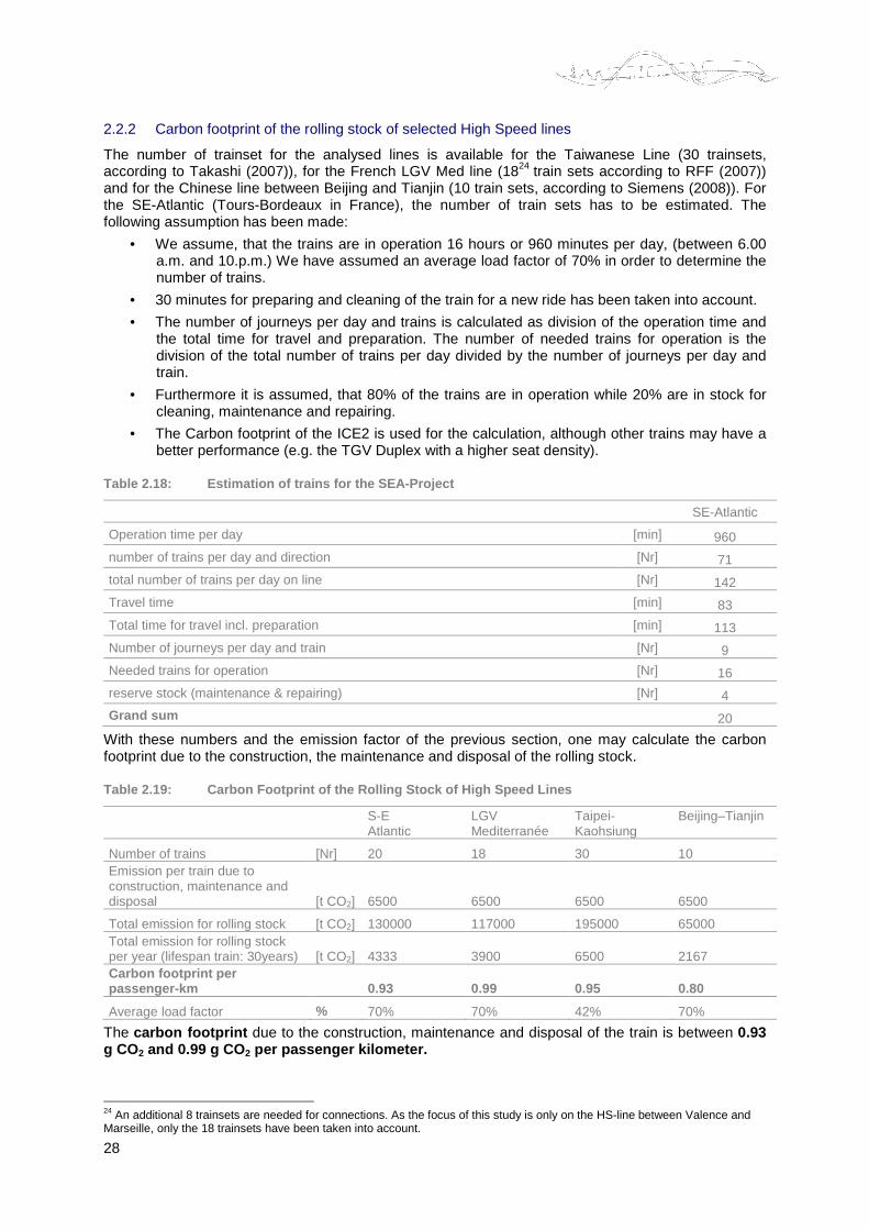
The emissions due to the production, maintenance and disposal of a train are around 6,000 – 7,000 t CO2. Please note that the carbon footprint per seatplace is in all trains (ICE 2, TGV Duplex, Shinkansen 200 & Shinkansen 300) in about the same order of magnitude. The difference of emissions between the first and the second generation of Shinkansen show that there is constant improvement in train construction.
Emissions from production, maintenance and disposal of train Shinkansen 300 ≈ 0.2 t eq. CO2 /seat-place/year < … < ICE2 ≈ 0.3 t eq. CO2 /seat-place/year
Figure 2.6: Comparison of carbon footprint from the train production among different HSR-train types
0.0%
25.0%
50.0%
75.0%
100.0%
ICE2 TGV Duplex Shinkansen 200 Shinkansen 300
t CO
2/ s
eat-p
lace
28
2.2.2 Carbon footprint of the rolling stock of selected High Speed lines
The number of trainset for the analysed lines is available for the Taiwanese Line (30 trainsets, according to Takashi (2007)), for the French LGV Med line (1824 train sets according to RFF (2007)) and for the Chinese line between Beijing and Tianjin (10 train sets, according to Siemens (2008)). For the SE-Atlantic (Tours-Bordeaux in France), the number of train sets has to be estimated. The following assumption has been made:
• We assume, that the trains are in operation 16 hours or 960 minutes per day, (between 6.00 a.m. and 10.p.m.) We have assumed an average load factor of 70% in order to determine the number of trains.
• 30 minutes for preparing and cleaning of the train for a new ride has been taken into account.
• The number of journeys per day and trains is calculated as division of the operation time and the total time for travel and preparation. The number of needed trains for operation is the division of the total number of trains per day divided by the number of journeys per day and train.
• Furthermore it is assumed, that 80% of the trains are in operation while 20% are in stock for cleaning, maintenance and repairing.
• The Carbon footprint of the ICE2 is used for the calculation, although other trains may have a better performance (e.g. the TGV Duplex with a higher seat density).
Table 2.18: Estimation of trains for the SEA-Project
SE-Atlantic
Operation time per day [min] 960
number of trains per day and direction [Nr] 71
total number of trains per day on line [Nr] 142
Travel time [min] 83
Total time for travel incl. preparation [min] 113
Number of journeys per day and train [Nr] 9
Needed trains for operation [Nr] 16
reserve stock (maintenance & repairing) [Nr] 4
Grand sum 20
With these numbers and the emission factor of the previous section, one may calculate the carbon footprint due to the construction, the maintenance and disposal of the rolling stock.
Table 2.19: Carbon Footprint of the Rolling Stock of High Speed Lines
S-E Atlantic
LGV Mediterranée
Taipei-Kaohsiung
Beijing–Tianjin
Number of trains [Nr] 20 18 30 10 Emission per train due to construction, maintenance and disposal [t CO2] 6500 6500 6500 6500
Total emission for rolling stock [t CO2] 130000 117000 195000 65000 Total emission for rolling stock per year (lifespan train: 30years) [t CO2] 4333 3900 6500 2167 Carbon footprint per passenger-km 0.93 0.99 0.95 0.80
Average load factor % 70% 70% 42% 70%
The carbon footprint due to the construction, maintenance and disposal of the train is between 0.93 g CO2 and 0.99 g CO 2 per passenger kilometer.
24 An additional 8 trainsets are needed for connections. As the focus of this study is only on the HS-line between Valence and Marseille, only the 18 trainsets have been taken into account.
29
Carbon Footprint of High Speed Rail
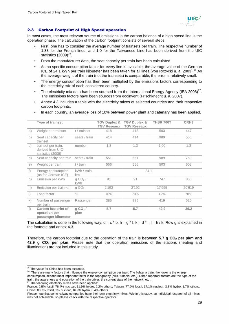
2.3 Carbon Footprint of High Speed operation
In most cases, the most relevant source of emissions in the carbon balance of a high speed line is the operation phase. The calculation of the carbon footprint consists of several steps:
• First, one has to consider the average number of trainsets per train. The respective number of 1.33 for the French lines, and 1.0 for the Taiwanese Line has been derived from the UIC statistics (2009)25.
• From the manufacturer data, the seat capacity per train has been calculated.
• As no specific consumption factor for every line is available, the average value of the German ICE of 24.1 kWh per train kilometer has been taken for all lines (von Rozycki u. a. 2003).26 As the average weight of the train (not the trainsets) is comparable, the error is relatively small.
• The energy consumption has then been multiplied by the emissions factors corresponding to the electricity mix of each considered country.
• The electricity mix data has been sourced from the International Energy Agency (IEA 2008)27. The emissions factors have been sources from ecoinvent (Frischknecht u. a. 2007).
• Annex 4.3 includes a table with the electricity mixes of selected countries and their respective carbon footprints.
• In each country, an average loss of 10% between power plant and catenary has been applied.
Type of trainset TGV Duplex &
TGV Reseaux TGV Duplex & TGV Reseaux
THSR 700T CRH3
a) Weight per trainset t / trainset 418 418 503 447
b) Seat capacity per trainset
seats / train 414 414 989 556
c) trainset per train, derived from UIC-statistics (2009)
number 1.3 1.3 1.00 1.3
d) Seat capacity per train seats / train 551 551 989 750
e) Weight per train t / train 556 556 503 603
f) Energy consumption (as for German ICE)
kWh / train-km
24.1
g) Emission per kWh g CO2 / kWh
91 91 747 856
h) Emission per train-km g CO2 2'192 2'192 17'995 20'619
i) Load factor % 70% 70% 42% 70%
k) Number of passenger per train
Passenger 385 385 419 526
l) Carbon footprint of operation per passenger kilometer
g CO2 / pkm
5.7 5.7 42.9 39.2
The calculation is done in the following way: d = c * b, h = g * f, k = d * I, l = h / k, Row g is explained in the footnote and annex 4.3.
Therefore, the carbon footprint due to the operation of the train is between 5.7 g CO 2 per pkm and 42.9 g CO2 per pkm . Please note that the operation emissions of the stations (heating and illumination) are not included in this study.
25 The value for China has been assumed. 26 There are many factors that influence the energy consumption per train: The lighter a train, the lower is the energy consumption, second most important factor is the topography (hills, tunnels, etc.). Other important factors are the type of the train, the awareness and education of the train driver, the current state of the network, etc… 27 The following electricity mixes have been applied: France: 9.5% fossil, 76.4% nuclear, 11.9% hydro, 2.2% others, Taiwan: 77.9% fossil, 17.1% nuclear, 3.3% hydro, 1.7% others, China: 80.7% fossil, 2% nuclear, 16.9% hydro, 0.4% others Please note that some railway companies have their own electricity mixes .Within this study, an individual research of all mixes was not achievable, so please check with the respective operator.
30
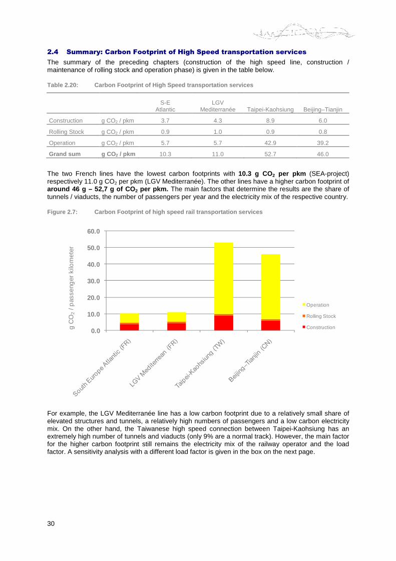
2.4 Summary: Carbon Footprint of High Speed transportation services
The summary of the preceding chapters (construction of the high speed line, construction / maintenance of rolling stock and operation phase) is given in the table below.
Table 2.20: Carbon Footprint of High Speed transport ation services
S-E Atlantic
LGV Mediterranée Taipei-Kaohsiung Beijing–Tianjin
Construction g CO2 / pkm 3.7 4.3 8.9 6.0
Rolling Stock g CO2 / pkm 0.9 1.0 0.9 0.8
Operation g CO2 / pkm 5.7 5.7 42.9 39.2
Grand sum g CO 2 / pkm 10.3 11.0 52.7 46.0
The two French lines have the lowest carbon footprints with 10.3 g CO2 per pkm (SEA-project) respectively 11.0 g CO2 per pkm (LGV Mediterranée). The other lines have a higher carbon footprint of around 46 g – 52,7 g of CO 2 per pkm. The main factors that determine the results are the share of tunnels / viaducts, the number of passengers per year and the electricity mix of the respective country.
Figure 2.7: Carbon Footprint of high speed rail tra nsportation services
0.0
10.0
20.0
30.0
40.0
50.0
60.0
Operation
Rolling Stock
Constructiong C
O2
/ pas
seng
er k
ilom
eter
For example, the LGV Mediterranée line has a low carbon footprint due to a relatively small share of elevated structures and tunnels, a relatively high numbers of passengers and a low carbon electricity mix. On the other hand, the Taiwanese high speed connection between Taipei-Kaohsiung has an extremely high number of tunnels and viaducts (only 9% are a normal track). However, the main factor for the higher carbon footprint still remains the electricity mix of the railway operator and the load factor. A sensitivity analysis with a different load factor is given in the box on the next page.
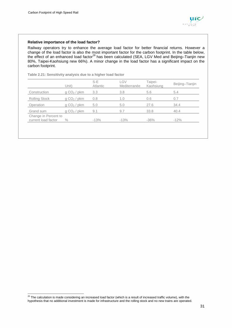
31
Carbon Footprint of High Speed Rail
Relative importance of the load factor? Railway operators try to enhance the average load factor for better financial returns. However a change of the load factor is also the most important factor for the carbon footprint. In the table below, the effect of an enhanced load factor28 has been calculated (SEA, LGV Med and Beijing–Tianjin new 80%, Taipei-Kaohsiung new 66%). A minor change in the load factor has a significant impact on the carbon footprint.
Table 2.21: Sensitivity analysis due to a higher loa d factor
Unit) S-E Atlantic
LGV Mediterranée
Taipei-Kaohsiung
Beijing–Tianjin
Construction g CO2 / pkm 3.3 3.8 5.6 5.4
Rolling Stock g CO2 / pkm 0.8 1.0 0.6 0.7
Operation g CO2 / pkm 5.0 5.0 27.6 34.4
Grand sum g CO2 / pkm 9.1 9.7 33.8 40.4 Change in Percent to current load factor % -13% -13% -36% -12%
28 The calculation is made considering an increased load factor (which is a result of increased traffic volume), with the hypothesis that no additional investment is made for infrastructure and the rolling stock and no new trains are operated.
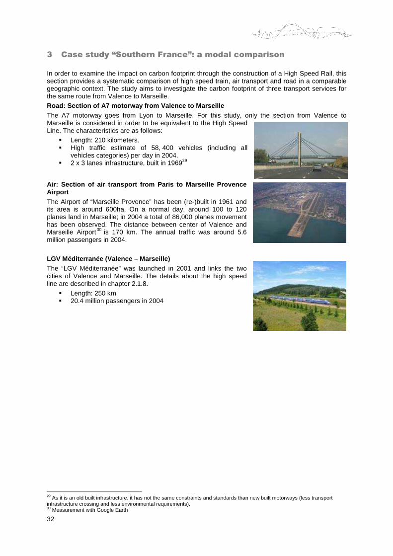
32
3 Case study “Southern France”: a modal comparison
In order to examine the impact on carbon footprint through the construction of a High Speed Rail, this section provides a systematic comparison of high speed train, air transport and road in a comparable geographic context. The study aims to investigate the carbon footprint of three transport services for the same route from Valence to Marseille.
Road: Section of A7 motorway from Valence to Marsei lle The A7 motorway goes from Lyon to Marseille. For this study, only the section from Valence to Marseille is considered in order to be equivalent to the High Speed Line. The characteristics are as follows:
� Length: 210 kilometers. � High traffic estimate of 58, 400 vehicles (including all
vehicles categories) per day in 2004. � 2 x 3 lanes infrastructure, built in 196929
Air: Section of air transport from Paris to Marseil le Provence Airport The Airport of “Marseille Provence” has been (re-)built in 1961 and its area is around 600ha. On a normal day, around 100 to 120 planes land in Marseille; in 2004 a total of 86,000 planes movement has been observed. The distance between center of Valence and Marseille Airport30 is 170 km. The annual traffic was around 5.6 million passengers in 2004.
LGV Méditerranée (Valence – Marseille) The “LGV Méditerranée” was launched in 2001 and links the two cities of Valence and Marseille. The details about the high speed line are described in chapter 2.1.8.
� Length: 250 km � 20.4 million passengers in 2004
29 As it is an old built infrastructure, it has not the same constraints and standards than new built motorways (less transport infrastructure crossing and less environmental requirements). 30 Measurement with Google Earth
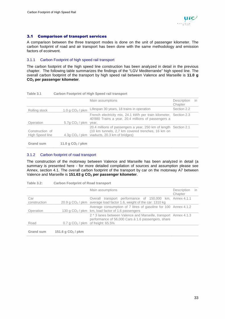
33
Carbon Footprint of High Speed Rail
3.1 Comparison of transport services
A comparison between the three transport modes is done on the unit of passenger kilometer. The carbon footprint of road and air transport has been done with the same methodology and emission factors of ecoinvent.
3.1.1 Carbon Footprint of high speed rail transport
The carbon footprint of the high speed line construction has been analyzed in detail in the previous chapter. The following table summarizes the findings of the “LGV Mediterranée” high speed line. The overall carbon footprint of the transport by high speed rail between Valence and Marseille is 11.0 g CO2 per passenger kilometer .
Table 3.1 Carbon Footprint of High Speed rail transp ort
Main assumptions Description in
Chapter
Rolling stock 1.0 g CO2 / pkm Lifespan 30 years, 18 trains in operation Section 2.2
Operation 5.7g CO2 / pkm
French electricity mix, 24.1 kWh per train kilometer, 40'880 Trains a year, 20.4 millions of passengers a year,
Section 2.3
Construction of High Speed line 4.3g CO2 / pkm
20.4 millions of passengers a year, 250 km of length (10 km tunnels, 2,7 km covered trenches, 16 km on viaducts, 20.3 km of bridges)
Section 2.1
Grand sum 11.0 g CO 2 / pkm
3.1.2 Carbon footprint of road transport
The construction of the motorway between Valence and Marseille has been analyzed in detail (a summary is presented here - for more detailed compilation of sources and assumption please see Annex, section 4.1. The overall carbon footprint of the transport by car on the motorway A7 between Valence and Marseille is 151.63 g CO2 per passenger kilometer .
Table 3.2: Carbon Footprint of Road transport
Main assumptions Description in
Chapter Car construction 20.9 g CO2 / pkm
Overall transport performance of 150,000 km, average load factor 1.6, weight of the car: 1310 kg
Annex 4.1.1
Operation 130 g CO2 / pkm Average consumption of 7 litres of gasoline for 100 km, load factor of 1.6 passengers
Annex 4.1.2
Road 0.7 g CO2 / pkm
2 * 3 lanes between Valence and Marseille, transport performance of 56,000 Cars à 1.6 passengers, share of freight: 65.5%
Annex 4.1.3
Grand sum 151.6 g CO 2 / pkm
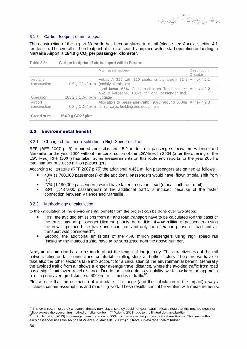
34
3.1.3 Carbon footprint of air transport
The construction of the airport Marseille has been analyzed in detail (please see Annex, section 4.1 for details). The overall carbon footprint of the transport by airplane with a start operation or landing in Marseille Airport is 164.0 g CO2 per passenger kilometer .
Table 3.3: Carbon footprint of air transport within Europe
Main assumptions Description in
Chapter Airplane construction 0.5 g CO2 / pkm
Airbus A 320 with 320 seats, empty weight 61 t (mainly aluminium)
Annex 4.2.1
Operation 163.2 g CO2 / pkm
Load factor: 65%, Consumption per Ton-kilometer: 452 g kerosene, 100kg for one passenger incl. luggage
Annex 4.2.2
Airport construction 0.3 g CO2 / pkm
Allocation to passenger-traffic: 90%, around 600ha for runways, building and equipment
Annex 4.2.3
Grand sum 164.0 g CO2 / pkm
3.2 Environmental benefit
3.2.1 Change of the modal split due to High Speed rail line
RFF (RFF 2007 p. 9) reported an estimated 15.9 million rail passengers between Valence and Marseille for the year 2004 without the construction of the LGV-line. In 2004 (after the opening of the LGV Med) RFF (2007) has taken some measurements on this route and reports for the year 2004 a total number of 20.368 million passengers.
According to literature (RFF 2007 p.75) the additional 4.461 million passengers are gained as follows:
� 40% (1,780,000 passengers) of the additional passengers would have flown (modal shift from air)
� 27% (1,190,000 passengers) would have taken the car instead (modal shift from road) � 33% (1,487,000 passengers) of the additional traffic is induced because of the faster
connection between Valence and Marseille.
3.2.2 Methodology of calculation
to the calculation of the environmental benefit from the project can be done over two steps:
� First, the avoided emissions from air and road transport have to be calculated (on the basis of the emissions per passenger kilometer). Only the additional 4.46 million of passengers using the new high-speed line have been counted, and only the operation phase of road and air transport was considered31,
� Second, the additional emissions of the 4.46 million passengers using high speed rail (including the induced traffic) have to be subtracted from the above number.
Next, an assumption has to be made about the length of the journey. The attractiveness of the rail network relies on fast connections, comfortable rolling stock and other factors. Therefore we have to take also the other sections take into account for a calculation of the environmental benefit. Generally the avoided traffic from air shows a longer average travel distance, where the avoided traffic from road has a significant lower travel distance. Due to the limited data availability, we follow here the approach of using one average distance of 600km for all modes of traffic32.
Please note that the estimation of a modal split change (and the calculation of the impact) always includes certain assumptions and modeling work. These results cannot be verified with measurements.
31 The construction of cars / airplanes already took place, so they could not count again. Please note that this method does not follow exactly the accounting method of “bilan carbon TM” (Ademe 2011) due to the limited data availability. 32 In Publictransit (2010) an average travel distance of 600km is mentioned for journey to Southern France. This means that each passenger uses the section of Valence to Marseille (250km) but travels in average 350km further.
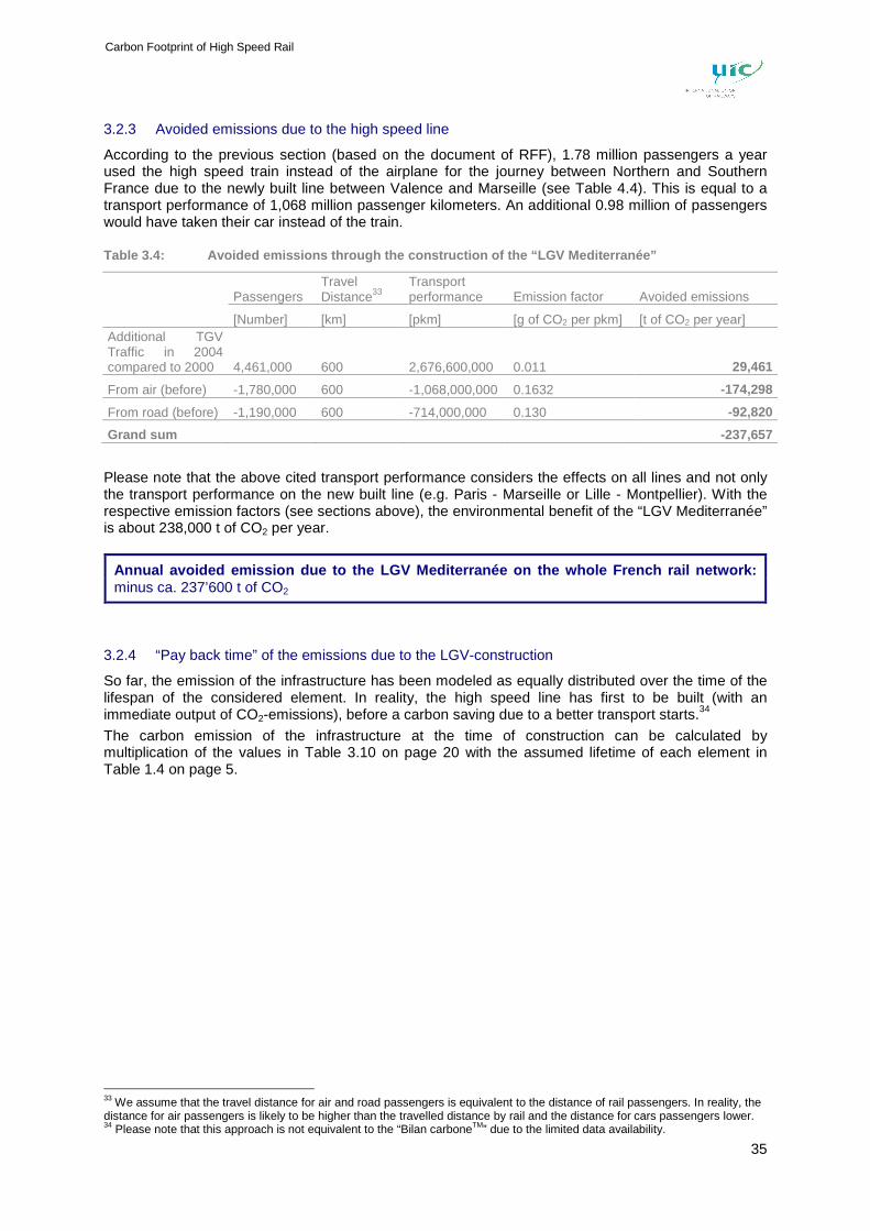
35
Carbon Footprint of High Speed Rail
3.2.3 Avoided emissions due to the high speed line
According to the previous section (based on the document of RFF), 1.78 million passengers a year used the high speed train instead of the airplane for the journey between Northern and Southern France due to the newly built line between Valence and Marseille (see Table 4.4). This is equal to a transport performance of 1,068 million passenger kilometers. An additional 0.98 million of passengers would have taken their car instead of the train.
Table 3.4: Avoided emissions through the constructi on of the “LGV Mediterranée”
Passengers Travel Distance33
Transport performance Emission factor Avoided emissions
[Number] [km] [pkm] [g of CO2 per pkm] [t of CO2 per year] Additional TGV Traffic in 2004 compared to 2000 4,461,000 600 2,676,600,000 0.011 29,461
From air (before) -1,780,000 600 -1,068,000,000 0.1632 -174,298
From road (before) -1,190,000 600 -714,000,000 0.130 -92,820
Grand sum -237,657
Please note that the above cited transport performance considers the effects on all lines and not only the transport performance on the new built line (e.g. Paris - Marseille or Lille - Montpellier). With the respective emission factors (see sections above), the environmental benefit of the “LGV Mediterranée” is about 238,000 t of CO2 per year.
Annual avoided emission due to the LGV Mediterranée on the whole French rail network: minus ca. 237’600 t of CO2
3.2.4 “Pay back time” of the emissions due to the LGV-construction
So far, the emission of the infrastructure has been modeled as equally distributed over the time of the lifespan of the considered element. In reality, the high speed line has first to be built (with an immediate output of CO2-emissions), before a carbon saving due to a better transport starts.34
The carbon emission of the infrastructure at the time of construction can be calculated by multiplication of the values in Table 3.10 on page 20 with the assumed lifetime of each element in Table 1.4 on page 5.
33 We assume that the travel distance for air and road passengers is equivalent to the distance of rail passengers. In reality, the distance for air passengers is likely to be higher than the travelled distance by rail and the distance for cars passengers lower. 34 Please note that this approach is not equivalent to the “Bilan carboneTM” due to the limited data availability.
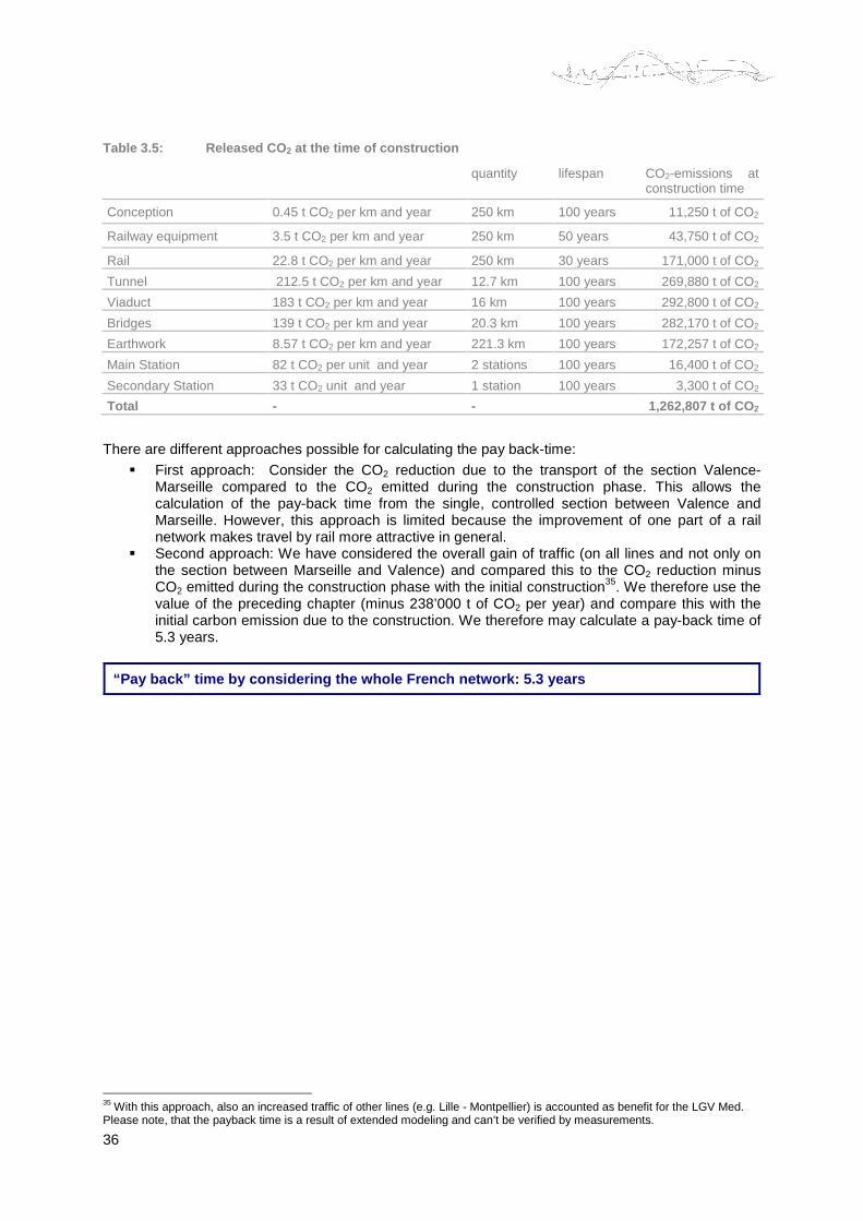
36
Table 3.5: Released CO 2 at the time of construction
quantity lifespan CO2-emissions at construction time
Conception 0.45 t CO2 per km and year 250 km 100 years 11,250 t of CO2
Railway equipment 3.5 t CO2 per km and year 250 km 50 years 43,750 t of CO2
Rail 22.8 t CO2 per km and year 250 km 30 years 171,000 t of CO2
Tunnel 212.5 t CO2 per km and year 12.7 km 100 years 269,880 t of CO2
Viaduct 183 t CO2 per km and year 16 km 100 years 292,800 t of CO2
Bridges 139 t CO2 per km and year 20.3 km 100 years 282,170 t of CO2
Earthwork 8.57 t CO2 per km and year 221.3 km 100 years 172,257 t of CO2
Main Station 82 t CO2 per unit and year 2 stations 100 years 16,400 t of CO2
Secondary Station 33 t CO2 unit and year 1 station 100 years 3,300 t of CO2
Total - - 1,262,807 t of CO 2
There are different approaches possible for calculating the pay back-time:
� First approach: Consider the CO2 reduction due to the transport of the section Valence-Marseille compared to the CO2 emitted during the construction phase. This allows the calculation of the pay-back time from the single, controlled section between Valence and Marseille. However, this approach is limited because the improvement of one part of a rail network makes travel by rail more attractive in general.
� Second approach: We have considered the overall gain of traffic (on all lines and not only on the section between Marseille and Valence) and compared this to the CO2 reduction minus CO2 emitted during the construction phase with the initial construction35. We therefore use the value of the preceding chapter (minus 238’000 t of CO2 per year) and compare this with the initial carbon emission due to the construction. We therefore may calculate a pay-back time of 5.3 years.
“Pay back” time by considering the whole French net work: 5.3 years
35 With this approach, also an increased traffic of other lines (e.g. Lille - Montpellier) is accounted as benefit for the LGV Med. Please note, that the payback time is a result of extended modeling and can’t be verified by measurements.
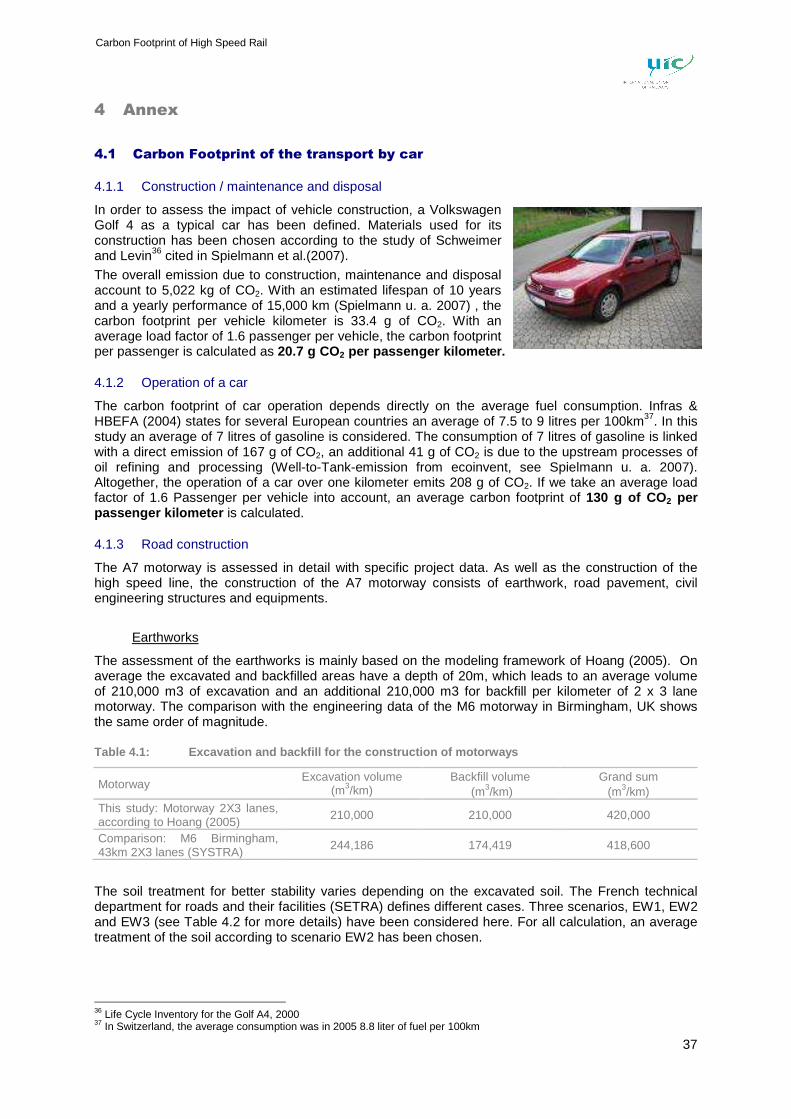
37
Carbon Footprint of High Speed Rail
4 Annex
4.1 Carbon Footprint of the transport by car
4.1.1 Construction / maintenance and disposal
In order to assess the impact of vehicle construction, a Volkswagen Golf 4 as a typical car has been defined. Materials used for its construction has been chosen according to the study of Schweimer and Levin36 cited in Spielmann et al.(2007).
The overall emission due to construction, maintenance and disposal account to 5,022 kg of CO2. With an estimated lifespan of 10 years and a yearly performance of 15,000 km (Spielmann u. a. 2007) , the carbon footprint per vehicle kilometer is 33.4 g of CO2. With an average load factor of 1.6 passenger per vehicle, the carbon footprint per passenger is calculated as 20.7 g CO2 per passenger kilometer.
4.1.2 Operation of a car
The carbon footprint of car operation depends directly on the average fuel consumption. Infras & HBEFA (2004) states for several European countries an average of 7.5 to 9 litres per 100km37. In this study an average of 7 litres of gasoline is considered. The consumption of 7 litres of gasoline is linked with a direct emission of 167 g of CO2, an additional 41 g of CO2 is due to the upstream processes of oil refining and processing (Well-to-Tank-emission from ecoinvent, see Spielmann u. a. 2007). Altogether, the operation of a car over one kilometer emits 208 g of CO2. If we take an average load factor of 1.6 Passenger per vehicle into account, an average carbon footprint of 130 g of CO 2 per passenger kilometer is calculated.
4.1.3 Road construction
The A7 motorway is assessed in detail with specific project data. As well as the construction of the high speed line, the construction of the A7 motorway consists of earthwork, road pavement, civil engineering structures and equipments.
Earthworks
The assessment of the earthworks is mainly based on the modeling framework of Hoang (2005). On average the excavated and backfilled areas have a depth of 20m, which leads to an average volume of 210,000 m3 of excavation and an additional 210,000 m3 for backfill per kilometer of 2 x 3 lane motorway. The comparison with the engineering data of the M6 motorway in Birmingham, UK shows the same order of magnitude.
Table 4.1: Excavation and backfill for the construct ion of motorways
Motorway Excavation volume
(m3/km) Backfill volume
(m3/km) Grand sum
(m3/km) This study: Motorway 2X3 lanes, according to Hoang (2005)
210,000 210,000 420,000
Comparison: M6 Birmingham, 43km 2X3 lanes (SYSTRA)
244,186 174,419 418,600
The soil treatment for better stability varies depending on the excavated soil. The French technical department for roads and their facilities (SETRA) defines different cases. Three scenarios, EW1, EW2 and EW3 (see Table 4.2 for more details) have been considered here. For all calculation, an average treatment of the soil according to scenario EW2 has been chosen.
36 Life Cycle Inventory for the Golf A4, 2000 37 In Switzerland, the average consumption was in 2005 8.8 liter of fuel per 100km
38
Table 4.2: Proposed soil treatment, depending on the types of the extracted soils, source: SETRA
Cases Types of extracted soils Application Quantity (m3/km) Preparation method before application
EW1 R21 (10%)
Sub grade 8,750 Cement treatment, 6% of the mass Backfill 6,250 No treatment
A2h (30%) Sub base 45,000 Lime treatment, 4% A2m (60%) Backfill 90,000 No treatment
EW2 R21 (10%)
Subgrade 8,750 Cement treatment, 6% Backfill 6,250 No treatment
A2h (30%) Sub base 45,000 Lime treatment, 2% A2m (60%) Backfill 90,000 No treatment
EW3 R21 (10%)
Sub grade 8,750 Cement treatment, 6% of the mass Backfill 6,250 No treatment
A2m (90%) Backfill 135,000 No treatment
Initial construction of road pavement
For road pavement, a flexible pavement with bituminous concrete has been chosen since it is widely used for new motorway construction in France (defined by SETRA). The motorway consists of the following elements:
� A surface course with 2 layers of asphalt concrete of 2,5 and 6,5cm � A base course composed of two layers of 13cm of road base asphalt � Emergency lanes and road divider composed of:
o A surface course of 4cm of asphalt concrete o A sub layer of 35cm of Gravel pit material.
As the A7 is 2 x 3 lanes motorway, the dimension of the structure is the following:
� 2X3 lanes of 3,5 meters each � 2 emergency lanes of 3 meters each � 1 road divider of 3 meters width
Table 4.3: Materials used for road construction
Gravel pit material (t/km)
Road Base Asphalt (t/km) Asphalt Concrete (t/km)
This study: 2X3 lane motorway modelled 6,716 12,831 5,993
Road pavement for maintenance
Concerning the maintenance of road pavement, the recommendation of SETRA for a 30 years period has been taken into account.
Table 4.4: Maintenance Policy for Bituminous Pavemen t – SETRA & LCPC (1998)
Time 9 years 17 years 25 years 30 years
Maintenance works for bituminous pavement
60% of surface, 4 cm asphalt concrete 40% of surface, 8 cm asphalt concrete
60% of surface, 4 cm asphalt concrete 40% of surface, 8 cm asphalt concrete
60% of surface, 4 cm asphalt concrete 40% of surface, 8 cm asphalt concrete
37% of surface, 4 cm asphalt concrete 27% of surface, 8 cm asphalt concrete
39
Carbon Footprint of High Speed Rail
Civil Engineering Structures
For civil engineering structure, an inventory of elevated structures and tunnels has been done according to measures on maps.
� Conventional structures such as bridges have been estimated with typical bridges based on data from the A41 motorway.
� Trenched and mined tunnels have been estimated according to their length with examples in the A29 and A41 motorways.
� Viaducts have been assessed according to their length with other examples on French motorways.
� Other structures as hydraulic culvert and animal passages have been assessed according to the recommendation of the SETRA.
The following table gives an overview about the used materials for civil engineering, the amount of steel compared to the M6 in Birmingham is lower due to les civil engineering structures.
Table 4.5: Materials for civil engineering structur es
Concrete (m3/km) Steel (reinforcement) (t/km)
Steel (structure) (t/km)
A7 (modeled) 1 422 135 143
M6 Birmingham 1 465 242 224
Equipment
Equipment of the A7 motorway have been investigated through:
� Crash barriers on road sides and civil engineering structures. Their type has been chosen according to standards defined by the SETRA. For road dividers, concrete separators have been chosen since they are often preferred to steel crash barriers on new motorways. Those safety equipments have been assumed to be set up for the total distance of the infrastructure.
� Toll stations have been assessed according to data for a toll station on the A41 motorway. � Fences comparable to those for High Speed Lines � Rest areas that have been inventoried. A typical type of rest area has been defined according
to real cases for the A4 motorway. Road structure is assumed to be the same than for the main road.
� Traffic signs have been assessed according to technical standards of distance between signs and the number of signs near road junctions from the French highway traffic act. Nevertheless many other signs exist and have not been taken into account.
Conclusion: Carbon Footprint
The emissions due to the construction of the motorway are about 73 t of CO2 per km and year. The main impact is from the earthwork38 and the pavement.
38 Please note that as mentioned in the previous paragraph for High Speed Line, the emissions from earthworks can be very different than the theorical ones used here.
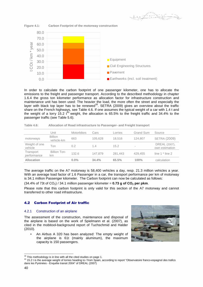
40
Figure 4.1: Carbon Footprint of the motorway constr uction
0.0
10.0
20.0
30.0
40.0
50.0
60.0
70.0
80.0
Equipment
Civil Engineering Structures
Pavement
Earthworks (incl. soil treatment)
t CO
2 / k
m *
yea
r
In order to calculate the carbon footprint of one passenger kilometer, one has to allocate the emissions to the freight and passenger transport. According to the described methodology in chapter 1.6.4 the gross ton kilometer performance as allocation factor for infrastructure construction and maintenance unit has been used: The heavier the load, the more often the street and especially the layer with black top layer has to be renewed39. SETRA (2009) gives an overview about the traffic share on the French highways, see Table 4.6. If one assumes the typical weight of a car with 1.4 t and the weight of a lorry 15.2 t40 weight, the allocation is 65.5% to the freight traffic and 34.4% to the passenger traffic (see Table 5.6).
Table 4.6: Allocation of Road infrastructure to Pass enger- and Freight transport
Unit Motorbikes Cars Lorries Grand Sum Source
motorways Billion vehicle-km 663 105,628 18,516 124,807 SETRA (2009)
Weight of one vehicle Ton 0.2 1.4 15.2 -
DREAL (2007), own estimation
Transport performance
Billion Ton-km
132.6 147,879 281,443 429,455 line 1 * line 2
Allocation 0.0% 34.4% 65.5% 100% calculation
The average traffic on the A7 motorway is 58,400 vehicles a day, resp. 21.3 million vehicles a year. With an average load factor of 1.6 Passenger in a car, the transport performance per km of motorway is 34.1 million Passenger kilometer. The Carbon footprint can now be calculated as follows:
(34.4% of 73t of CO2) / 34.1 million passenger kilometer = 0.73 g of CO 2 per pkm .
Please note that this carbon footprint is only valid for this section of the A7 motorway and cannot transferred to other road infrastructure.
4.2 Carbon Footprint of Air traffic
4.2.1 Construction of an airplane
The assessment of the construction, maintenance and disposal of the airplane is based on the work of Spielmann et al. (2007), as cited in the mobitool-background report of Tuchschmid and Halder (2010).
• An Airbus A 320 has been analyzed: The empty weight of the airplane is 61t (mainly aluminum), the maximum capacity is 150 passengers.
39 This methodology is in line with all the cited studies on page 1. 40 15.2 t is the average weight of lorries heading to / from Spain, according to report “Observatoire franco-espagnol des trafics dans les Pyrénées - Enquête transit 2004” of DREAL (2007)
41
Carbon Footprint of High Speed Rail
• As an airplane transports in every flight passengers and freight, the carbon impact has also to be split up. In this case, the allocation factor is one transported ton of goods, a passenger incl. luggage has an assumed weight of 100kg.
• In an Intra-European flight, an average load-factor of 65% (or 98 Passengers) has been assumed.
According to Spielmann et al. (2007), the carbon footprint of the construction and the maintenance of an airplane is 0.48 g of CO 2.
4.2.2 Operation of the airplane
For the operation phase of the airplane, the same data source has been used. Per ton of air cargo (passenger & freight) on an Intra-European Flight, on average 452g of kerosene is necessary for the transport of one ton kilometer. This is equivalent with a direct output of 1.426kg of CO2, and upstream emissions of 206 g CO2. The grand sum is 1,632 g CO2. As one passenger is assumed to weigh 100kg (person plus luggage), the carbon footprint per passenger kilometer is 163.2 g of CO 2.
4.2.3 Construction of Airport
The airport of Marseille has been analyzed in detail. It consists of the earthwork and pavement for the runways, equipments and the construction of the buildings. Please note, that the important phase of Airport operation (electricity, heating of buildings, water and glycol for deicing has not been considered.
Earthworks & Runway Pavement
In order to assess earthworks, an area of 600 ha has been defined according to maps, corresponding to runways, buildings area and parking areas. For this perimeter, 2 meters depth for excavation and backfill have been considered. The soil treatment has been assessed with the same assumptions as for road transport. One assumes that the cement and bituminous strata is renewed every 30 years.
A cement concrete structure has been chosen for pavement, runways, taxiways and aircraft parking. It can be described as follow:
� 40 cm of cement concrete � 10 cm of bituminous concrete � 20 cm of treated gravel pit � 35 cm of treated sediments
Buildings & Equipments
The inventory of materials used for the construction of the buildings has been estimated according to the surface and types of buildings with a ratio of materials per square meter. The area occupied by buildings has been assessed according to the plans of Marseille airport. Four types of buildings have been defined that correspond to existing examples on other airports:
� Terminal buildings � Hangar with steel structure � Hangar with concrete structure � Medium flat building
Materials for the control tower construction are assumed to be the same as for Brussels airport control tower for which precise data have been collected.
The main equipment taken into account is the fences and parking areas. Parking areas are been modeled with the same requirements than for motorway parking areas.
Carbon footprint
The emission due to the construction of the airport is about 2,200 t of CO2 per unit and year. Also here, the main impact is from pavement and earthwork.
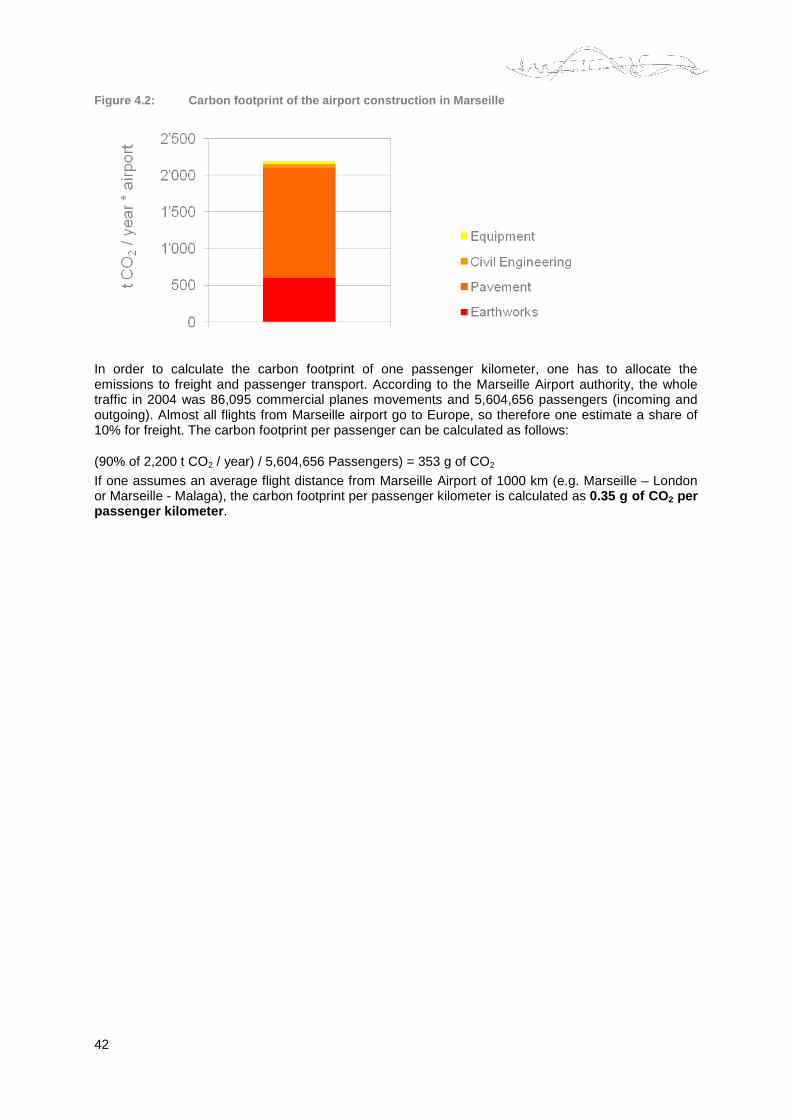
42
Figure 4.2: Carbon footprint of the airport constru ction in Marseille
In order to calculate the carbon footprint of one passenger kilometer, one has to allocate the emissions to freight and passenger transport. According to the Marseille Airport authority, the whole traffic in 2004 was 86,095 commercial planes movements and 5,604,656 passengers (incoming and outgoing). Almost all flights from Marseille airport go to Europe, so therefore one estimate a share of 10% for freight. The carbon footprint per passenger can be calculated as follows:
(90% of 2,200 t CO2 / year) / 5,604,656 Passengers) = 353 g of CO2
If one assumes an average flight distance from Marseille Airport of 1000 km (e.g. Marseille – London or Marseille - Malaga), the carbon footprint per passenger kilometer is calculated as 0.35 g of CO 2 per passenger kilometer .
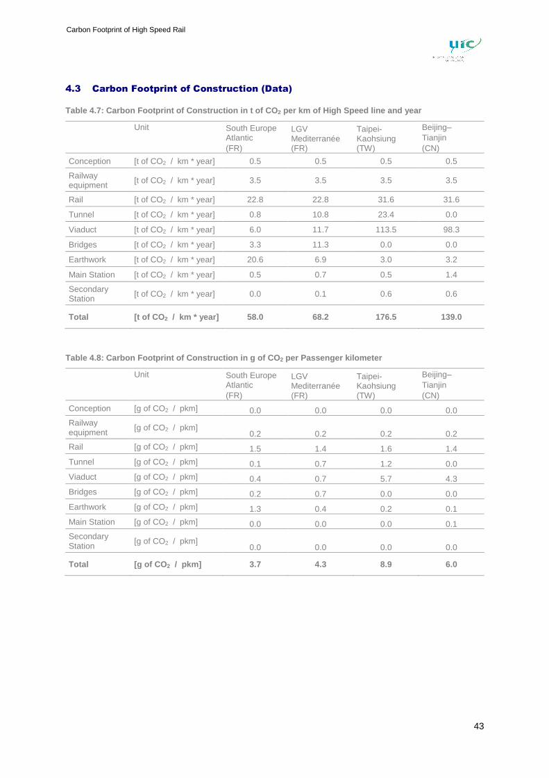
43
Carbon Footprint of High Speed Rail
4.3 Carbon Footprint of Construction (Data)
Table 4.7: Carbon Footprint of Construction in t of CO2 per km of High Speed line and year
Unit South Europe Atlantic (FR)
LGV Mediterranée (FR)
Taipei-Kaohsiung (TW)
Beijing– Tianjin (CN)
Conception [t of CO2 / km * year] 0.5 0.5 0.5 0.5
Railway equipment [t of CO2 / km * year] 3.5 3.5 3.5 3.5
Rail [t of CO2 / km * year] 22.8 22.8 31.6 31.6
Tunnel [t of CO2 / km * year] 0.8 10.8 23.4 0.0
Viaduct [t of CO2 / km * year] 6.0 11.7 113.5 98.3
Bridges [t of CO2 / km * year] 3.3 11.3 0.0 0.0
Earthwork [t of CO2 / km * year] 20.6 6.9 3.0 3.2
Main Station [t of CO2 / km * year] 0.5 0.7 0.5 1.4
Secondary Station [t of CO2 / km * year] 0.0 0.1 0.6 0.6
Total [t of CO 2 / km * year] 58.0 68.2 176.5 139.0
Table 4.8: Carbon Footprint of Construction in g of CO2 per Passenger kilometer
Unit South Europe Atlantic (FR)
LGV Mediterranée (FR)
Taipei-Kaohsiung (TW)
Beijing– Tianjin (CN)
Conception [g of CO2 / pkm] 0.0 0.0 0.0 0.0
Railway equipment
[g of CO2 / pkm] 0.2 0.2 0.2 0.2
Rail [g of CO2 / pkm] 1.5 1.4 1.6 1.4
Tunnel [g of CO2 / pkm] 0.1 0.7 1.2 0.0
Viaduct [g of CO2 / pkm] 0.4 0.7 5.7 4.3
Bridges [g of CO2 / pkm] 0.2 0.7 0.0 0.0
Earthwork [g of CO2 / pkm] 1.3 0.4 0.2 0.1
Main Station [g of CO2 / pkm] 0.0 0.0 0.0 0.1
Secondary Station
[g of CO2 / pkm] 0.0 0.0 0.0 0.0
Total [g of CO 2 / pkm] 3.7 4.3 8.9 6.0
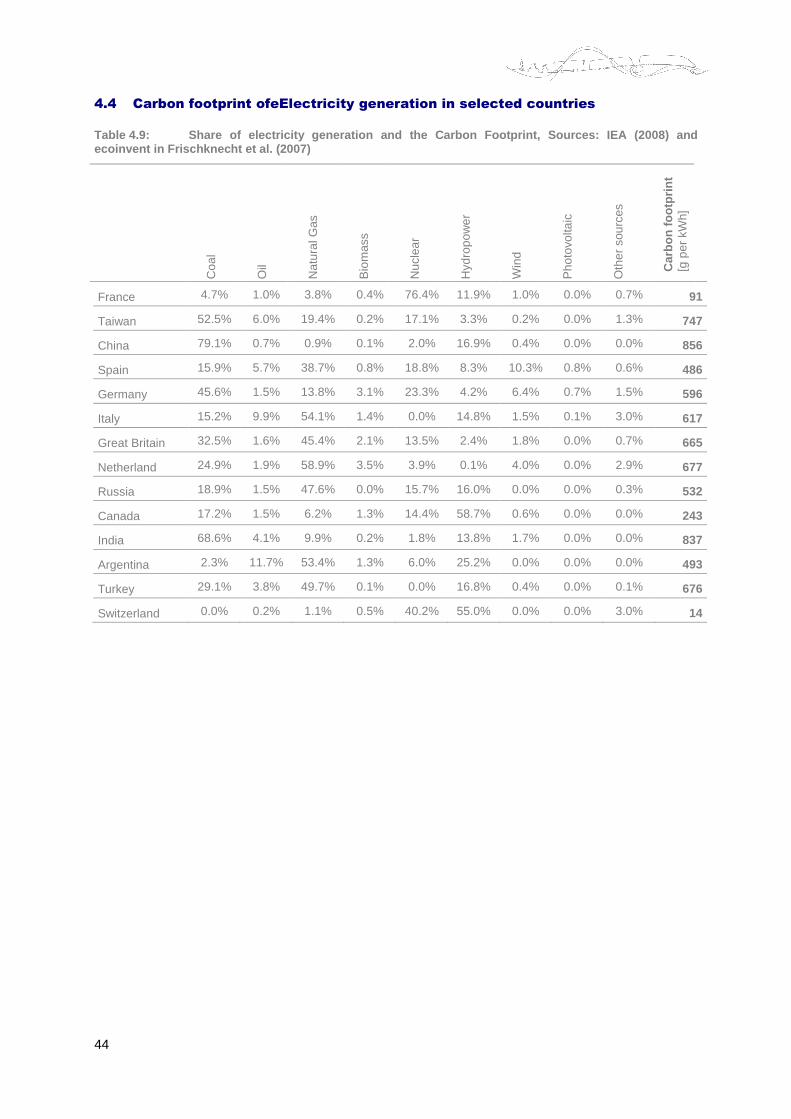
44
4.4 Carbon footprint ofeElectricity generation in selected countries
Table 4.9: Share of electricity generation and the C arbon Footprint, Sources: IEA (2008) and ecoinvent in Frischknecht et al. (2007)
Coa
l
Oil
Nat
ural
Gas
Bio
mas
s
Nuc
lear
Hyd
ropo
wer
Win
d
Pho
tovo
ltaic
Oth
er s
ourc
es
Car
bon
foot
prin
t [g
per
kW
h]
France 4.7% 1.0% 3.8% 0.4% 76.4% 11.9% 1.0% 0.0% 0.7% 91
Taiwan 52.5% 6.0% 19.4% 0.2% 17.1% 3.3% 0.2% 0.0% 1.3% 747
China 79.1% 0.7% 0.9% 0.1% 2.0% 16.9% 0.4% 0.0% 0.0% 856
Spain 15.9% 5.7% 38.7% 0.8% 18.8% 8.3% 10.3% 0.8% 0.6% 486
Germany 45.6% 1.5% 13.8% 3.1% 23.3% 4.2% 6.4% 0.7% 1.5% 596
Italy 15.2% 9.9% 54.1% 1.4% 0.0% 14.8% 1.5% 0.1% 3.0% 617
Great Britain 32.5% 1.6% 45.4% 2.1% 13.5% 2.4% 1.8% 0.0% 0.7% 665
Netherland 24.9% 1.9% 58.9% 3.5% 3.9% 0.1% 4.0% 0.0% 2.9% 677
Russia 18.9% 1.5% 47.6% 0.0% 15.7% 16.0% 0.0% 0.0% 0.3% 532
Canada 17.2% 1.5% 6.2% 1.3% 14.4% 58.7% 0.6% 0.0% 0.0% 243
India 68.6% 4.1% 9.9% 0.2% 1.8% 13.8% 1.7% 0.0% 0.0% 837
Argentina 2.3% 11.7% 53.4% 1.3% 6.0% 25.2% 0.0% 0.0% 0.0% 493
Turkey 29.1% 3.8% 49.7% 0.1% 0.0% 16.8% 0.4% 0.0% 0.1% 676
Switzerland 0.0% 0.2% 1.1% 0.5% 40.2% 55.0% 0.0% 0.0% 3.0% 14
45
Carbon Footprint of High Speed Rail
4.5 Bibliography
Bibliography from Editor
Ademe, 2011. Bilan Carbone - Tout savoir sur le Bilan Carbone. Available at: http://www2.ademe.fr/servlet/KBaseShow?sort=-1&cid=96&m=3&catid=15730 [Zugegriffen Juli 7, 2011]. Bögl GmbH, 2008. Slab Track China, Available at: http://www.max-boegl.de/boeglnet/web/show.jsp?nodeId=1000245&lang=de.
DREAL, 2007. Observatoire franco-espagnol des trafics dans les pyrénées - Enquête transit 2004. Available at: http://www3.midi-pyrenees.equipement.gouv.fr/rubrique.php3?id_rubrique=586&id_article=1739.
Frischknecht, R., Tuchschmid, M. & Faist Emmenegger M., Bauer C. and Dones R., 2007. Strommix, Dübendorf, CH: Swiss Centre for Life Cycle Inventories.
Gong, J., 2011. Full steam ahead on China’s high-speed rails, Available at: http://en.huanqiu.com/opinion/commentary/2011-03/628507.html.
Hoang, T., 2005. Tronçon autoroutiers: une méthodologie de modélisation environementale et économique pour different scenarios de construction et d’entretien,
IEA, 2008. IEA Energy Statistics. Available at: http://www.iea.org/stats/prodresult.asp?PRODUCT=Electricity/Heat.
INFRAS & HBEFA, 2004. HBEFA: Handbuch für Emissionsfaktoren im Strassenverkehr,
LGV2030, 2011. LGV2030: LE TGV MEDITERRANEE. Available at: http://lgv2030.free.fr/ligne1.htm#Med.
PCR, 2008. Product Category Rules for preparing an Environmental Product Declaration (EPD) for Interurban railway transport services of passengers, Railway transport services of freight and Railways. PCR 2009:03,
Publictransit US, J., 2010. High-Speed Rail Passenger Traffic Density Statistics, Available at: http://www.publictransit.us/ptlibrary/CoxVranich.htm [Zugegriffen Mai 8, 2011].
RFF, 2007. Bilan LOTI de la LGV Méditerranée,
RFF, 2011. South Atlantic Europe High Speed Line - Réseau Ferré de France. Available at: http://www.rff.fr/en/railway-network/projects/new-railways-lines-2916/south-europe-atlantic-high-speed-line.
von Rozycki, C., Koeser, H. & Schwarz, H., 2003. Ecology Profile of the German High-speed Rail Passenger Transport System, ICE. Int J LCA, 8(2), S.83-91.
Schmied & Mottschall, 2010. Treibhausgasemissionen durch die Schieneninfrastruktur und Schienen-fahrzeuge in Deutschland,
SETRA, 2009. Sondage de circulation 2004 - 2005: Document de synthèse. Available at: http://www.setra.equipement.gouv.fr/Sondage-de-circulation-2004-2005.html.
Siemens, 2008. Mobility-Newsletter: High speed train goes into service in China,
Spielmann, M., Dones, R. & Bauer, C., 2007. Life Cycle Inventories of Transport Services. Final report ecoinvent v2.0 No. 14., Dübendorf, CH: Swiss Centre for Life Cycle Inventories.
Takashi, S., 2007. High Speed railways in Asia: Taiwan High Speed Rail,
Tang, S.M.T., 2006. How front end factors affect project outcomes: a look at foru infrastructure projects in Asia, Available at: http://crgp.stanford.edu/publications/working_papers/with_old_cover_page/Tang_frontend_factors_project_outcomes.pdf.
Tricoire, J. & Soulié, C., 2002. Le grand livre du TGV, La Vie du Rail.
Tuchschmid, M., 2010. Carbon Footprint of High-Speed railway infrastructure (Pre-Study), Zürich: Commissioned by International Union of Railways (UIC).
Tuchschmid, M. & Halder, M., 2010. mobitool – Grundlagenbericht: Hintergrund, Methodik & Emissionsfaktoren. Available at: www.mobitool.ch.
46
UIC, 2011. High speed lines in the world - UIC - International Union of Railways. Available at: http://www.uic.org/spip.php?article573. UIC, 2007. International Railway statistics, Paris.
UIC, 2009. International Railway statistics, Paris.
Bibliography from SYSTRA
ADEME, Guide des facteurs d’émissions, Technical Report, ADEME, January 2007
AIR FRANCE , L’impact environnemental en chiffres, Press Report, Air France,
C.Alvarez & JF.Pochet , A29, recyclage à fort taux : une première !, Review Article, Travaux, n°776, P45-47, June 2001
ASF, L’autoroute A89 d’ouest en est, Review Article, Travaux, n°768, P24-33, October 2 000
ASF, ASF démarre des travaux d’aménagement de l’A7 pour renforcer la sécurité de ses clients et de ses ouvriers, press article, ASF, September 2003
ASF, Programme A7/A9 mobilité durable, Press article, ASF, April 2009
ASF, A87 Angers La Roche/Yon, Press Article, ASF, July 2008
ASF, Nos engagements développement durable : bilan 2008 engagements 2009, Activity report, ASF, 2009
ASFA , la sécurité un état d’esprit, un état de faits, Press Report, ASFA, May 2004
ASFA , Chiffres clés 2004, Activity report, ASFA, 2005
C.Bassi , Présentation de la méthodologie bilan carbone appliquée à une infrastructure routière, powerpoint presentation, CETE Méditerranée
BELGOCONTROL , La tour de contrôle de Bruxelles National, Press Report, Belgocontrol, Mars 2005
DN. Bilow, GM. Randich , Slab Track For The Next 100 Years, Press Article, Portland Cement Association
H.Birgisdottir, Life Cycle assessment model for road construction and used of residues from waste incineration, Thesis, Institute of Environment & Ressources, Technical University of Denmark, July 2005
BITUME.INFO, Aéroports : Liège choisit le bitume pour rénover sa piste, Press Article, Bitume info, n°10, P8-10, October 2005
M.Bonnet & P.Bourdon , Construire l’A41 Nord en 29 mois : un défis technique et opérationnel A41 Nord Annecy-Genève, Review Article, Travaux, n°850, P26-30, Mars 2008
47
Carbon Footprint of High Speed Rail
E.Bouffard-Savary , Tendances et perspectives du transport aérien : éclairages sur Marseille-Provence dans un contexte européen et mondial, Symposium on air transport development and noise management, DGAC, November 2007
BRITPAVE , Slab Track – Life-Cycle energy study of railway track beds, Technical Report, Britpave, 2007
P.Chardard , A29 un chantier de surface et de traitement, Review Article, Travaux, n°777, P16-19, July-August 2001
M.Chester & A.Horvath , Environmental Life-cycle Assessment of Passenger Transportation - An Evaluation of Automobles, Buses, Trains, and Aircraft in the United States, Research Report, University of California – Berkeley, 2008
CIMBETON, Sécurité routière : les dispositifs de retenue en béton, Press Article, Routes, n°95, P7-14, Mars 2006
CNDP, Le trafic, les niveaux de service et les impacts à horizon 2020 : la situation de référence, Working Paper, Commission particulière du débat public - politique des transports de la vallée du Rhône – arc languedocien, P79-84, 2006
JP Cureau & JM Bedmar , Tehran-Qom-Esfahan High Speed Railway Line Summary Report About HIGH-SPEED FLEET Classification For The H.S.R. Systems In The World, Technical Report, SYSTRA, July 2007
Y.Deniel & Y.Schaller & F.Caron , L’autoroute des estuaires A84 section Coulvain-Guilberville, Review Article, Travaux, n°740, P34-38, Mars 1998
DGAC, Les chaussées aéronautiques, Technical Report, DGAC, January 2007
DGAC & AEROPORTS DE PARIS , Aéroport Paris Charles de Gaulle – Information sur les travaux – Fermeture de la piste 1 du 17 Juillet au 25 août 2006, Press Report, DGAC & Aéroports de Paris, 2006
DGAC & LCPC , Chaussées aéronautiques en béton hydraulique, Technical Report, DGAC & LCPC, February 2000
L.De Vèzes , Oulmes – A10 : la route des Estuaires par l’A83, Press article, Forum Chantier n°2, May/June 2000
I.Douglas & N.Lawson , Airport construction: materials use andgeomorphic change, School of Geography, University of Manchester, Research Report, Journal of Air Transport Management, n°9, P177–185, 2003
J.Fairburn & Prof G.Pugh , An assessment of the carbon footprint of the M6 Toll Motorway in the UK, Reasearch Report, Institute for Environment, Sustainability and Regeneration, Staffordshire University
JL.Garcia De Viedma , Caracteristicas generales de la linea de Alta Velocidad, Research Report, Revista de obras publicas, Issue 3.386, Pages 19-39, April 1999
M.Gillam & BF.Townsend (2005), Orient Express, Press article, Civil Engineering, Pages 50-57, April 2005
48
G.Griffiths , La Autopista M6 Toll En Birmingham, Press Report, Ove Arup & Partners, September 2004
J.Gonnet & F.Debain & C.Massenet , Aéroport de Roissy : Piste 4 et voies de circulation, Press Article, Travaux, n°750, P41-45, February 1999
J.Guibert & D.Goumard , Le contournement Nord d’Angers, Review Article, Travaux, n°826, P25-36, January 2006
J.Guichard & P.Chardard , A29 Ouest Neufchâtel-en-Bray/Amiens, Review Article, Travaux, n°810, P20-23, July-August 2004
T.Hoang , Tronçons autoroutiers: une méthodologie de modélisation environnementale et économique pour différent scénarios de construction et d’entretien, Thesis, Ecole Centrale de Nantes & Université de Nantes, November 2005
C.Hugrel & R.Joumard , Directives et facteurs agrégés d’émission des véhicules routiers en France de 1970 à 2025, Research Report, INRETS, June 2006
A.Jullien , Questions environnementales liées au traitement de sols, Symposium on poor soil enhancement, LCPC, 2008
H.Kato & N.Shibahara & M.Osada & Y.Hayashi , A Life Cycle Assessment For Evaluating Environmental Impacts Of Inter-Regional High-Speed Mass Transit Projects, Journal of the Eastern Asia Society for Transportation Studies, Vol. 6, 2005, Pages 3211 – 3224
E.Lavallée & P.Bonel , Géotechnique, matériaux et chaussées A41 Nord Annecy-Genève, Review Paper, Travaux, n°850, p88-96, Mars 2008
C. K. Lee & J. Y. Lee & Y. K. Kim , Comparison of environmental loads with rail track systems using simplified life cycle assessment (LCA), Research Article, Urban Transport, Issue XIV, P367-372, 2008
LES PROFILS DU CENTRE , Glissière double DE2, product declaration, Les profiles du Centre, September 2003
LES PROFILS DU CENTRE , Glissière double DE4, product declaration, Les profiles du Centre, July 2003
LES PROFILS DU CENTRE , Glissière double GS2 amovibles, product declaration, Les profiles du Centre, September 2003
LES PROFILS DU CENTRE , Glissière simple GS2, product declaration, Les profiles du Centre, September 2003
J.Martin , A51-Les terrassements, Review Article, Travaux, n°757, P56-59, October 1 999
G.Martinetti , Le Bilan Carbone des Projets Ferroviaires, Research Report, Ecole Nationale des Ponts et Chaussées & SYSTRA, 2008
Y.Meunier , Autoroute A29 Amiens/St Quentin : innover pour économiser…, Review Article, Travaux, n°776, P34-39, June 2001
49
Carbon Footprint of High Speed Rail
MINISTERE DE L’EQUIPEMENT, DU LOGEMENT, DE L’AMENAG EMENT DU TERRITOIRE, ET DES TRANSPORTS, Dispositifs de retenue des véhicules – conditions d’agrément et d’emploi, technical report, Ministère de l’équipement, du logement, de l’aménagement du territoire et des transports, May 1988
S.Miura & H.Takai & M.Uchida & Y.Fukada , The Mechanism of Railway Tracks, Review Article, Japan Railway & Transport Review, March 1998, Pages 38-45
T.Miyauchi & T.Nagatomo & T.Tsujimura & H.Tsuchiya , Fundamental LCA of Shinkansen Vehicles, Review article, QR of RTRI, Volume 40, n°4, Decembe r 1999, Pages 204-209
E.Niemann , L’énergie Grise Dans La Filiere Batiment Et Travaux Publics, Working Paper, Laboratoire Central des Ponts et Chaussées
A.Perazio , Atténuer le bruit, Review Article, Travaux, n°757, P67, October 1999
G.Point & G.Cartoux , Autoroute A77 la déviation de Nevers, Review Article, Travaux, n°740, P41-46, Mars 1998
RAZEL , Barrière de péage générale sur l’A41, Razel Tribune, n°48, P15, September 2007
G. Rebitzer, T. Ekvall, R. Frischknecht, D. Hunkeler, G. Norris, T. Rydberg, W. -P. Schmidt, S. Suh, B. P. Weidema, D. W. Pennington , Life cycle assessment: Part 1: Framework, goal and scope definition, inventory analysis, and applications, Research Report, Environment International, Volume 30, Issue 5, Pages 701-720, 2004
F.Renaud , Les ouvrages d’art courants, Review Paper, Travaux, n°757, P54-55, October 199 9
RFF & SNCF, Bilan LOTI de la LGV Méditerranée, ex post evaluation report, June 2007
G.Riondy & B.Mitte & M.Petit & C.Thomasson , Autoroute A89 Mussidan – Périgueux Travaux et terrassements spéciaux, Review Article, Travaux, n°810, P59-67, July-Augu st 2004
SANEF, Inauguration de l’A29, liaison Amiens – Neufchâtel-en-Bray, Press Report, SANEF, January 2005
S.Sayagh , Approche multicritères du recyclage de co-produits dans des chaussées, Thesis, Laboratoire Central des Ponts et Chaussées, December 2007
SETRA, Equipements des autoroutes non concédées, technical note, June 1994
GW. Schweimer & M.Levin , Life Cycle Inventory for the Golf A4, Research report, Volkswagen & University of Kassel, 2000
SNCB, L’architecture de la gare se dévoile, Press article, Liège Guillemins, Issue 3, June 2003
STAC, Entretien des chaussées aéronautiques, Technical Report, STAC, June 1999
E.Storksen & D.Buffet & G.Pian & J.Kessler & M.Bocq ueraz , La barrière de péage pleine voie de Villy-le-Pelloux Un chantier au coeur du chantier A41 Nord Annecy-Genève, Review Article, Travaux, n°850, P105-109, Mars 2008
50
E.Storksen & A.Legeay & N.Caris & S.Grange , Les ouvrages d’art hors viaducs A41 Nord Annecy-Genève, Review Article, Travaux, n°850, p77-87, Mars 2008
STAC, Réfection des chaussées aéronautiques, Technical Report, STAC, June 1999
STAC, Conception des chaussées aéronautiques, Technical Report, STAC, June 1999
D.Tissier , Le Technicentre Est Européen, un atelier nouvelle génération, Research Article, Revue Générale des Chemins de Fer, Pages 65-77, May 2007
H Ueda & T Miyauchi & T Tsujimura , Application of lifecycle assessment to Shinkansen vehicles and cross ties in Japan, Review Article, Proceedings of the Institution of Mechanical Engineers, Part F: Journal of Rail and Rapid Transit, P271-278, 2003
C.Von Rozicky & H.Koeser & H.Schwarz , Ecology Profile of the German High-speed Rail Passenger Transport System, ICE, Research article, LCA Case Studies – Railway Passenger Transport, 2003