Carbon Dioxide Evolution from the Floor of Three Minnesota ForestsAuthor(s): W. A. ReinersReviewed work(s):Source: Ecology, Vol. 49, No. 3 (May, 1968), pp. 471-483Published by: Ecological Society of AmericaStable URL: http://www.jstor.org/stable/1934114 .Accessed: 03/02/2012 14:04

Your use of the JSTOR archive indicates your acceptance of the Terms & Conditions of Use, available at .http://www.jstor.org/page/info/about/policies/terms.jsp

JSTOR is a not-for-profit service that helps scholars, researchers, and students discover, use, and build upon a wide range ofcontent in a trusted digital archive. We use information technology and tools to increase productivity and facilitate new formsof scholarship. For more information about JSTOR, please contact support@jstor.org.

Ecological Society of America is collaborating with JSTOR to digitize, preserve and extend access to Ecology.

http://www.jstor.org

Late Spring 1968 CARBON DIOXIDE EVOLUTION RATES 471

number from non-saline soils, suggesting an eco- typic difference. Established plants can withstand soil salinization uip to 18-21 atm before 50% of them die. Of all the species tested, this one has the greatest potential for osmoregulation.

Elynmus cinereuis germinates moderately well in NaCI and in natural salts up to an osmotic pres- sure of 4.5 atm. There was no consistent differ- ence in the behavior of seeds collected from saline and non-saline habitats; this suggests high physi- ologic plasticity within one geographic ecotype.

The capacity of a species to accommodate in- creasing salinization of soil with NaCl was in- creased when another species was rooted in the same soil.

ACK NOWLEDGM ENTS

The author wishes to express his appreciation to Prof. R. Daubenmire for providing all possible facilities and for his guidance during this work. Thanks are also ex- tended for his review of the manuscript.

LITERATURE CITED

Ahi, W. M., and W. L. Powers. 1938. Salt tolerance of plants at various temperatures. Plant Physiol. 13: 767-789.

Ayers, A. D., and H. E. Hayward. 1948. A method for measuring the effect of soil salinity on germina- tion. Soil Sci. Soc. Amer. Proc. 13: 224-226.

Gauch, H. G., and C. H. Wadleigh. 1944. Effect of high concentration of salts on growth of bean plants. Bot. Gaz. 105: 379-387.

Gauch, H. G., C. H. Wadleigh, and Virginia Davis. 1943. The trend of starch reserves in bean plants before and after irrigation of a saline soil. Proc. Amer. Soc. Hort. Sci. 43: 201-209.

Harris, F. S. 1915. Effects of alkali salts in soils on germination and growth of crops. J. Agr. Res. 5: 1-53.

. 1920. Soil alkali. Wiley, New York. 258 p. Harris, F. S., and D. W. Pittman. 1918. Soil factors

affecting the toxicity of alkali. J. Agr. Res. 15: 287- 319.

Kearney, T. H., and C. S. Schofield. 1936. The choice of crops for saline lands. U. S. Dep. Agr. Circ. 404. 24 p.

Moodie, C. D., H. W. Smith, and R. L. Hausenbuiller. 1963. Laboratory manual for soil fertility. Wash- ington St. Univ., Dept. Agronomy, Pullman, Washing- ton. 198 p.

Rudolfs, W. 1925. Influence of water and salt solu- tion upon absorption and germination of seeds. Soil Sci. 20: 15-37.

Schimper, A. F. W. 1903. Plant geography upon physi- ological basis. Transl. by R. Fisher. Clarendon Press, Oxford. 839 p.

Shive, J. W. 1916. The effect of salt concentration on the germination of seeds. New Jersey Agr. Exp. Sta. Ann. Rep. 37: 455457.

Strogonov, B. P. 1964. Physiological basis of salt tolerance of plants. Translated from Russian. Daniel Davy & Co., Inc., New York. 279 p.

Uhvits, R. 1946. Effect of osmotic pressures on water absorption and germination of alfalfa seeds. Amer. J. Bot. 33: 278-285.

Waisel, Y. 1958. Germination behavior of some halc- phytes. Bull. Res. Council Israel (D) 6: 187-188.

CARBON DIOXIDE EVOLUTION FROM THE FLOOR OF THREE MINNESOTA FORESTS

W. A. REI N ERS

Department of Botany, Unizversity of Minnesota Minneapolis, Minnesotal

(Accepted for publication February 23, 1968)

Abstract. Carbon dioxide evolution rates from forest floors, measured approximately weekly for 54 weeks in oak forest, marginal fen, and cedar swamp, were closely related to soil temperature and secondarily to moisture conditions. As a result, rmicroclimatic and drainage characteristics of the three forests produced seasonal differences in carbon release. However, compensatory factors produced nearly equal cumulative annual totals of CO2 evo- lution. Total CO2 evolution was over three times higher than expected from an equivalent amount of carbon release from annual litter fall. Respiration by tree roots was suspected as the major contributor to this disparity although methodological problems related to flow rate are still open to question.

INTRODUCTION

Net primary production of forest ecosystems meets two principal fates: it is stored in the mas- sive standing crop of producers, or it falls to the ground as litter and becomes incorporated into the forest floor. In contrast with some aquatic and

'Present address: Department of Biological Sciences, Dartmouth College, Hanover, N. H. 03755.

grassland systems, direct grazing of living pro- ducer tissue represents a minor pathway of en- ergy flow under normal circumstances (Bray 1964).

Since energy flow via the detritus pathway pre- dominates in forests, the forest floor is the major arena of heterotroph activity and may be con- sidered a heterotrophic subsystem of the forest as

472 W. A. REINERS Ecology, Vol. 49, No. 3

a whole. Tracing energy flow through the myriad populations inhabiting the forest floor is an exceed- ingly difficult task (Birch and Clark 1953), and a thorough assessment of energy release and trans- fer by these populations may not be achieved for many years. This difficulty is offset, in part, by the fact that heterotroph metabolism is centralized in the forest floor and the sum of energy release by all populations may be measured by monitoring some by-product of respiration from the forest floor itself.

One approach for measuring this summed en- ergy release is to measure rates of carbon dioxide evolution from forest floors. This approach pos- sesses several difficulties. Any carbon compounds released other than CO2, such as acids or alcohols to ground water or methane or carbon monoxide to the atmosphere, represent a loss of energy by exportation as well as leakage of an indicator of partial oxidation. These errors cause an under- estimation of rates of energy release. On the other hand, CO2 release from tree root respiration may cause an overestimation of rates of activity in the forest floor alone.

Carbon dioxide evolution is itself difficult to measure accurately. It varies through the year and within more short-term periods (Douglas and Tedrow 1959, Witkamp 1966). Conditions im- posed by measurement apparatus may create seri- ous deviations from normal conditions for hetero- troph activity. In spite of these difficulties, CO2 evolution probably remains the most convenient means for estimating heterotroph metabolism and is receiving continued attention. If absolute values are unreliable, at least such data can be useful in comparing rates of biological activity under different conditions in contrasting ecosys- tems. Such comparative values are useful diag- nostic parameters of ecosystem types, aiding in describing patterns of energy flow or factors controlling rates of decay and nutrient release. Hopefully, techniques may finally be improved to the point that data derived by some CO. moni- toring system will provide reliable absolute values of energy flow.

This paper describes a comparative study of CO2 evolution in three forest ecosystems of di- verse structure. The study was designed to meet four objectives: (1) determine if there are sig- nificant differences in annual, cumulative CO2 evolution from diverse forest floors; (2) measure significant temporal variations in CO. evolution rates attributable to forest characteristics such as time of litter input, dates of freezing and thawing, and moisture effects due to differences in drain- age; (3) determine which measurable environ- mental factors might be most useful in predicting

rates of C02 evolution; and (4) test whether the system devised in this study might provide reliable absolute data on rates of energy flow through heterotrophs in the forest floor.

THE STUDY AREA

The forests studied are located at Cedar Creek Natural History Area, Anoka Co., Minn., about 48 km north of Minneapolis. They are contigu- ously distributed along a topographic gradient established by a sandy peninsula nearly surrounded by a peat-filled basin (Fig. 1). The slopes of the

inEthe Ceal Cre aua itryAeAoaC.

white ~ ~ 4. oa9Qecu raan ae brh(e

0'a

SW -.Sec. 27. 060 .0 20 30

4ll 906rfea feelliin ordrobdniy

T. 34 N, R 23 Wse 000

FIG. 1. Location of the 80- by 60-rn study site along the slope of a peninsula extending into a cedar swamp in the Cedar Creek Natural History Area, Anoka Co., Minn.

peninsula are forested by northern pin oak (Quer- cus ellipsoida-lis),2 red maple (Acer urn) white oak (Quercuas cba), and paper birch (Be- tela papyrifera) in declining order of density. Juneberry (Aselanchier sp.) and ironwood (Os- trya virginiana), representing a broken subcanopy, are scattered throughout the forest type. A high shrub layer of American hazel (Corylfs atbrain- cana) and a low shrub layer of blueberry (Vac- ciniuo angustifoliut) are only sporadically repre- sented. A wide variety of herbs, of which Penn- sylvania sedge (Carex pensylvanica) is most prominent, forms an herbaceous stratum.

At the intersection of the peninsula slope and the surface of organic sediments of the basin is located a lagg or marginal fen (sensu Conway 1959) of 20 m width. The dominant trees of the community in descending order of density are black ash (Fraxinzis nigra), speckled alder (Al- nits rugosa), red maple, white cedar (Thiija occi- dentalis), and American elm (Ulinus amtericana). Most of this community features a dense layer of several species of ferns of which cinnamon fern

2 Plant nomenclature follows Fernald (1950).

Late Spring 968 CARBON DIOXIDE EVOLUTION RATES 473

(Osmunda cinnamomea), interrupted fern (0. Claytoniana), and lady fern (Athyrium Filix- femina) are most prominent. Under the ferns and in open places, sedges and grasses form a low herb layer.

The basin forest is dominated by white cedar and paper birch but has a good representation of marginal fen species. The herb layers are scanty although mosses are locally abundant.

The floor of the oak forest is somewhat hetero- geneous in development. Although all areas have a 3- to 4-cm L layer and 0.6-cm F layer, some sections feature a well-defined H layer and char- acteristics of a weak mor, while nearby, other sections feature deep A1 horizons with no H layer-characteristics of a mull. In the fen a nearly homogeneous black humus, 15-30 cm deep, underlies a light litter and thick sward of sedges. The humus is abruptly separated from a dark- brown, mottled sand which blends into a well- gleied, gray sand of unknown depth. The forest floor in the cedar swamp features thin L and F layers overlying peat in various degrees of humifi- cation extending down to 1.3 m.

METHODS

Six plots used for measuring CO2 evolution were located in randomized block fashion in each of the three communities. Each plot consisted of a painted, steel sleeve 20 cm wide, 50 cm long, and 20 cm deep which was inserted into the forest floor until the top edges were slightly above the top of the litter. The sleeves were emplaced on 2 August 1965.

Carbon dioxide evolution from the isolated sec- tions of forest floor in these sleeves was measured by tightly covering the sleeve with an opaque cover and making it a part of an open flow system (Fig. 2). Ambient air collected from a 6-m tower on the crest of the peninsula was pumped through polyvinyl chloride tubing to the plot and into a port on one end of the sleeve cover. The air was distributed across the 20-cm width of the plot by a manifold and flowed along the length of the plot to be exhausted at the opposite end. A sample of air collected at the exhaust end was picked up by a manifold and pumped back up to the peninsula crest. A positive air pressure was always maintained over the forest floor section to prevent suction of CO2 from the pore spaces of the forest floor and soil. The system was designed to simulate laminar air flow at realistic velocities across the litter surface.

Air being pumped into and withdrawn from the plot was sampled for CO2 content with a Beck- man, model 15-A, infra-red gas analyzer. Flow rate was measured with a Brooks rotameter at the

AMBIENT AIR INTAKE EXHAUST iW lfRA-R(D GAS ANALYZER

[51 ~ ~~~~~~~~ lLOW ME T7ER |

/% | ~~~DRYING COLU

( ~~~~PORTS ON COVER MAY BE OPENEO TO MEASURE AIR VELOCITIES.

FLOW RATE AIR TEMPERATURES MEASURED AT EXHAUST PORTS THIS POINT UN COVER

I - E . .*-SLEEVE COVER LITTER LATER - U R . - FERMENTATION LATER . : . .- .. * A, HORIZON .. . . .....SLEEVE 20C

H 0~~~~~~ A2 -81 HORIZONS U 0 0 U

5D CM

FIG. 2. The open flow system used for measuring CO2 evolution from forest floors.

plot input and air temperature with a Tri-R electronic thermometer. With these measurements and a measurement of the CO2 enrichment of air passing over the plot, a calculation of CO2 evolu- tion could be made. Flow rates ranged from 19 to 25 liters/min which corresponded to measured air velocities under the cover of the plot of 5.6-9.2 cm/sec. Air flowed across plots from 2 to 5 min before analysis began, and air was sampled until a steady level of CO2 output was attained. This usually required a minimum of 6 min.

Carbon dioxide evolution measurements began 27 August 1965 and terminated 20 September 1966. Measurements were made on all plots be- tween 0900 and 1700 hours approximately weekly except for a period between 14 December 1965 and 19 March 1966, in which the soil was frozen. Soil temperatures were measured at 5 and 15 cm depths, 5-10 cm from each end of the plot sleeve with a Tri-R soil probe at the time of each sam- pling. Soil moisture was not measured, but a soil moisture index was constructed with precipi- tation data collected at Cedar Creek Natural His- tory Area and air temperatures recorded by an official weather station in Cambridge, Minn., lo- cated 16 km north of the study area. Potential evapotranspiration was calculated by the Thornth- waite method (Thornthwaite 1948). Assuming an average, well-drained soil contains 10 cm of water in the rooting zone at field capacity, a run- ning balance was calculated from outgo through evapotranspiration, and from income through pre- cipitation. An increase of moisture greater than 10 cm was assumed to be lost from the rooting zone to the water table so the maximum of mois- ture was always 10 cm. Water was assumed to be limiting to evapotranspiration when the stored moisture in the soil was depleted.

Obviously a particular moisture index had dif-

474 W. A. REINERS Ecolog,. Vol. 49. No. 3

ferent meanings for each forest type since the fen and swamp were on poorly drained sites. As an example, samples of the Al horizon (or depth equivalent in the fen and swamp) were collected from randomly chosen locations in each forest type on 22 August 1966, a date for which the mois- ture index was calculated as 1.0 cm. Moisture content by volume in the oak forest was 7%c, while in the fen and swamp it was 50%. Although the index was a crude, relative estimate of mois- ture conditions, it was easily calculated and the best estimate available under the circumstances.

Two methodological problems were investigated. One problem was the uncertainty of whether ini- tial rates could be sustained for several hours under the conditions of measurements. If they could not, this would be some indication that the measurement procedure was producing evolution values which could not be considered normal for an open forest floor. The second problem involved the question of whether flow rates influenced evo- lution rates. To resolve these problems, CO2 evolution was monitored continuously for several hours at varying flow rates from one representa- tive plot in each forest type. Flow rates were

alternated between the normal 24 liters/min and lower or higher rates. Lengths of time for the runs ranged from 3.2 to 6.1 hr. Air velocities were estimated as means of measurements taken at three points across the middle of the plots with an Alnor hot-wire anemometer.

RESULTS

Soil temperature and moisture index Soil temperatures declined steadily from Sep-

tember 1965 to January 1966 (Fig. 3). December was characterized by frost and thaw, and early in January 1966 the soils were frozen and covered with snow. Soils remained frozen until mid- March at which time temperatures rose rapidly in the oak forest, which had an open canopy and slight, south-facing slope. Temperatures rose more slowly in the fen, which was partially shaded from the sun by the dense cedar foliage of the swamp on its south side. Soil temperature rose very slowly in the heavily-shaded cedar swamp and did not reach the levels of the oak forest and fen until mid-June. It must be emphasized that these temperatures are averages of 12 measure- ments at 5-cm depth and 12 at 15 cm in each of

22.0r

20.01 ------ A 1

0 8 .0 I

1.6.0 V

Cr 14.0 \

CL 4.0 j W 8.0 - D~~~~~~~~~~~~~~~~~~~~~0' p' '4

2.0

0~~~~~ OAK

0.8

; 1.01 0OAK

2 0.6~ 01 I

0 ~ ~ ~ ~ ~ ~ ~ ~ ~ ~ ~ ~ ~ ~ ~ ~~~~~~ 0.4 \

(3 C?\ '~~~~~~~~~~~~~ . 'z>I ~~~~~~~~~5.09- 0.2-0z

K. ~~~~~~~~~~~~~~~~~2.5 0.0 -uW

SEPT. OCT. NOV. DEC. JAN. FEB. MAR. APR. MAY JUNE JULY AUG. SEPT. CEa.

FIG. 3. Above: Soil temperature and moisture index during the 54 xweek study period. Below: CO2 evolu- tion rates, together with bars indicating precipitation events.

Late Spring 1968 CARBON DIOXIDE EVOLUTION RATES 475

the forest types. During the period of soil warm- ing, surface temperatures were often warmer than indicated by the average, which was partially based on temperatures from frozen levels at 15 cm or less. On the other hand, soil temperatures were higher at 15 cm than 5 cm during the autumn cooling period.

From July to September 1966 soil temperatures for the three forests were very similar. In gen- eral, oak forest temperatures were highest and cedar swamp temperatures the lowest. More striking than differences between forests was the high-amplitude fluctuation in soil temperatures of all the forests. These fluctuations are partially correlated with precipitation events (Fig. 3). Sizable storms depressed soil temperatures to nearly equal levels in all three forests; drying periods correlated with higher temperatures and greater differences between soil temperatures of the three forests.

Statistical significance of differences in average soil temperatures between forest types was esti- mated at the .90 confidence level with the Tukey multiple comparison test when sample numbers from all forest types were equal and with Scheff6's method of multiple comparison when sample num- bers were unequal. Both methods are described by Scheff6 (1959, p. 66-75). Results of these tests are summarized in Table 1. Moisture index values were inversely correlated with soil temperatures. High moisture conditions prevailed at low tem- peratures, while at high temperatures, moisture levels tended to be low.

TABLE 1. Significant differences between soil tempera- tures of forest types at .90 confidence level (o oak forest, f = marginal fen, s = cedar swamp)

No. of No. of meas- % measure- Significant occurrences urements in ments sig-

Period differences in period period nificant

1 Sept o>f 5 42 1965 - f>o 1 8 11 Jan f>s 4 12 33 1966 s>f 1 8

0>8 9 75

19 Mar o>f 8 67 1966 - f>s 8 12 67 27 June 0>8 10 83 1966

6 July o>f 2 22 1966 - f>s 3 9 33 31 Aug 0>8 3 33 1966

COB evolution In general, CO2 evolution rates parallel soil

temperatures (Fig. 3). This is particularly evi- dent during the cooling period from September 1965 to January 1966. Evolution rates of CO2

were measured at or very near zero on 11 January and were assumed to be negligible until March. From 19 March to 5 May evolution rates in- creased slowly, and there was no regular differ- ence in output between the three forest types. Beginning about 14 May CO2 evolution rates began to rise rapidly, correlating with higher soil temperatures. Between 27 June and 20 Septem- ber evolution rates peaked and gradually descended in a pattern of high amplitude oscillations which corresponded with rainfall and fluctuations in soil temperatures. Throughout this period the oak forest or the cedar swamp produced the high- est evolution rates while the marginal fen was generally lowest.

TABLE 2. Significant differences between CO2 evolution rates of forest types at .90 confidence level (o = oak forest, f = marginal fen, s = cedar swamp)

No. of No. of meas- % measure- Significant occurrences urements in ments sig-

Period differences in period period nificant

I Sept o>f 1 9 1965- f>s 1 11 9 11 Jan s>f 2 18 1966 8>0 2 18

19 Mar o>f 5 42 1966 - f>s 1 8 27 June s>f 1 12 8 1966 8>0 1 8

0>8 4 33

6 July o>f 2 10 20 1966 - 0>5 1 10 31 Aug 1966

Statistical significance of differences between CO2 evolution rates of the three forest types was tested by the same methods as described for soil temperatures (Table 2). The spring warming period is the period of greatest frequency of sig- nificant differences; the most frequent of these differences are those of oak over swamp and oak over fen. The fall cooling period has the second highest frequency of significant differences, and of these, two-thirds are accounted for by cases in which the swamp shows significantly higher out- puts than the other two types. Only two signifi- cant contrasts were found in the summer, both involving predominance of oak output over that of the fen or swamp. Twenty-one per cent of possible comparisons of CO2 evolution rates over the year showed statistically significant differ- ences compared with 55% for soil temperatures.

The relationships between seasonal effects and CO2 evolution can best be seen in a graph of cumulative CO2 evolution (Fig. 4). The three forests show equal decreases in output until early December when the cedar swamp decreases more

476 W. A. REINERS Ecology, Vol. 49, No. 3

2600 o

2600g~

t 2400 O 3-O OAK FOREST X 0---0 MARGINAL FEN

2200 0--V CEOAR SWAMP a

2 1000 1 00 a

0 1400

200

SEPT. OCT. NOV. DEC. JAN. PER. MAR. APR. MAT JUNE JOLT AUG.

FIG. 4. Cumulative CO2 evolution from three forest floors over a 12-month period. The increase from Jan- uary to March in the marginal fen is questionable (see text) .

rapidly than oak or fen forests. Oak forest and cedar swamp outputs were uniformly low over the winter period while fen output continued at mod- erate rates. By 19 March cumulative CO2 output for the fen was approximately 200 gm/in2 greater than the oak and cedar forests. It should be emphasized that this disparity in cumulative CO2 evolution over the winter was based on the unusu- ally high rates measured for the fen on 19 March (see Fig. 3). It is possible that these high rates were not representative of winter behavior and cumulative fen output did not exceed oak and swamp to the extent shown in Fig. 4. On the other hand, the soil at 15 cm was slow to freeze in the autumn in the fen and was well thawed at depth by 19 March, indicating that perhaps the heat content of ground water just below the sur- face maintained soil temperatures above freezing, which in turn maintained moderate rates of micro- bial metabolism.

In the spring period, cumulative output in the oak forest and cedar swamp increased rapidly until they matched, and then exceeded, fen out- put in early and midsummer. During summer months rates of increase in cumulative CO2 were about equal in oak and swamp forest and greater than that of the fen. At the conclusion of the 12- month period cumulative CO2 output was 2,912, 2,710, and 2,592 gm/in2 in the oak, swamp, and fen forests, respectively. None of the differences between these values were significant at the .90 confidence level.

Multiple regression analysis

The marked relationships between CO2 evolu- tion rates, soil temperatures, and moisture led to an attempt to estimate the control these factor had

on CO2 evolution rates and to produce a model for predicting rates on the basis of these factors. Carbon dioxide rates plotted against soil tempera- tures revealed a curvilinear, apparently exponen- tial relationship (Fig. 5). Typically, variation was greater at high temperatures presumably be- cause moisture conditions were more variable in warmer periods than during the colder months. Semi-log plots of CO2 rates against soil tempera- ture produced linear curves. Wiant (1967c) has illustrated such an exponential relationship be- tween 200 and 40?C.

I.600 0

1. 400 A Z0" C B

A A I 200

-~~~~~~~~~~~ A~~~~~~~~~~ * 1.000 0

0 A 0 A 0A

o~~~~~~~~~~~~~~~ A

, .800 v 0 0?

.000

0 A 0 0

o1 .600 *0 L a01 <J .400 0 O

0A ?0 ?0 A

A 5 ~ ~ ~ 0 SI 0 P E T ,

0 .0

.2G0 A 0tb?. & o

0 Zl 4.0 6.0 o.0 10.0 A2.0 i4.0 u6 0 o18.0 20.0 2fom SOIL TEMPERATURE, -C

FIG. 5. The relation between C02 evolution rates from the oak forest floor and soil temperature. Zones A and B are contiguous, 10-m belts located parallel to contour lines in the oak forest. Zone A is directly upslope from zone B.

The moisture index was so highly correlated with temperatures that it was difficult to attain meaningful plots of CO2 rates versus moisture index. All that was discernible was that increas- ing moisture index values tended to correlate with increasing CO2 evolution rates. A curvilinear in- crease in CO2 output over a range of increasing moisture content has been shown under laboratory conditions by Wiant (1967d).

On the basis of these preliminary examinations, the following working model was tested:

In CO2= C +B1 (T) + B2 (MI)

where C= constant, B1 = coefficient for soil tem- perature, T = soil temperature in ?C, B2 = co- efficient for moisture index, and MI = moisture index. This model was equivalent to the following equation which demonstrates exponential relation- ships between CO2 and temperature and mois- ture:

CO2 =e C + B1 T + B2 MI

Multiple regression values were obtained for each individual plot with the total data collected on that plot throughout the 54-week period. The average value for regression statistics from six

Late Spring 1968 CARBON DIOXIDE EVOLUTION RATES 477

TABLE 3. Results of multiple regression analysis on CO2 evolution rates from forest floors of three forest ecosys- tems according to the model: In CO2 = C + B1 temperature) + B2 (moisture index). Values are averages of individual analyses on six plots per forest type. Dispersion around means are indicated by ? one standard error of means.

Coefficients and measures of dispersion Oak forest Marginal fen Cedar swamp

C (constant) ....................................... -2.63? .19 -2.07 ?.20 -2.06?.19 B1 (temp. coefficient) ........... .................... 0.11 ?0.01 0.07 ? .01 0.08? .01 Standard deviation, B1. . 0.01 0.02 0.02 B1/standard deviation of B1.9.55? .92 4.35? .65 5.92?1.3 Partial correlation (In CO2 and temp.) . . . 0.85? .02 0.60? .07 0.67 ? .09 B2 (moisture index coefficient) ....... ................ 0.04 ?.006 +0.03? .02* +0.04 + .007* Standard deviation, B2 ............................. 0.02 0.03 0.02 B2/standard deviation of B ............ ............... 1.98? .25 1.38? .40 1.36 ? .24 Part al correlation, (In CO2 and moisture) .... ........ 0.33? .04 0.23? .07 0.24? .04 Simpile correlation-temp/moisture ...... .............. 0.74 ? .02 0.76 ? .001 0.77 ? .02 Multiple correlation coefficient ...... ................ 0.90? .02 0.76? .05 0.83 ? .04 Standard error of estimate .......................... 0.29? .02 0.41? .04 0.38? .10

Coefficient negative four of six times in fen, one of six times in swamp.

plots in each forest type are shown in Table 3. All values listed except standard error of estimate and simple correlation of temperature and mois- ture index are highest for the oak forest type, while the same values for the fen and swamp are lower than oak and more or less equal with each other. This suggests that the total heterotroph metabolism in the oak forest floor is more sensi- tive to changes in temperature and moisture and that this behavior can be more readily explained by, and predicted with, these parameters than the generally wetter, and apparently more stable fen and swamp forest floor ecosystems.

The average constants (C) and coefficient B1 and B2 for the three forest types were compared for significant differences using the Tukey mul- tiple comparison test. All three constants and all three temperature coefficients (B1) were sig- nificantly different from each other at the .90 con- fidence level. There was no significant difference between any of the moisture index coefficients.

It may be ecologically significant that the near- zero average moisture index coefficients for fen and swamp types resulted not so much from the low responses to moisture changes but rather from the fact that coefficients for some of the plots in these wetter sites were negative, and the averages of positive and negative values were near zero. Both the fen and swamp show hummock and hol- low microtopography, and both hummocks and hollows were represented by plots. A subjective evaluation of each plot in terms of hummock or hollow condition coincided with the appropriate sign of B2 in eight of 12 cases.

The predicted CO2 evolution rates according to the model were computed and graphically com- pared with observed rates. The cedar swamp plot used for the comparison shown in Fig. 6 was chosen as an example because multiple correlation

coefficients for cedar swamp plots were interme- diate between oak and fen plots, and because this plot was representative of cedar swamp plots with regard to the statistics listed in Table 3. The mul- tiple correlation coefficient for the equation gen- erated from data from this plot was 0.88. The oscillations of predicted and observed curves match well; the fit is somewhat better in mid- summer than in spring or fall.

1 -1 * OSERVEO CO2 EVOLUTION PLOT 6-2

1D0---- OPREOtCTED CO2 EVOLUTION CEDAR SWAMP

OO ~ ~ ~ ~ NOE _. . . . . . . ..I

V~ ~ 96 16

0.8

0 0.7

06

?0.5

04

a024

0 2

0 040 60 80 100 120 140 160 180 200 220 240 260 280 300 320 340 340 IJAN. FES MAR.I APR. I MAY IJUNE I JULY IAUrG SEPT. IOCT. I NOV IOEC I

i966 1 1965

FIG. 6. Observed and predicted CO2 evolution rates from a typical plot in the cedar swamp.

Although the fits of predicted and observed data for the model were satisfactory from a predictive point of view, it was clear that the supposedly controlling factors, temperature and moisture, were in reality correlated with time, and other factors correlated with tinte might have some controlling influence. To test the influence of a simple time factor, a second model incorporating an expression for seasonal changes was also tested by multiple regression analysis. This analysis indicated that although a considerable amount of variation at- tributed to temperature in the original model was incorporated into the expression for time in the second model, multiple-correlation coefficients

478 W. A. REINERS Ecology, Vol. 49, No. 3

TABLE 4. Carbon dioxide evolution rates for three plots representing oak forest (A-2), marginal fen (D-4), and cedar swamp (F-2) forest floors over ranges of time and at various air-flow rates

Flow rate (liter/ CO2 evolution

Time interval (hr) min) (gm/M2 per hour)

PLOT A-2 (14 July 1966) .0 - .75 .2............ . 013.4 .61 .75-1.17 .............. 14.0 1.88

1.17-1.50 .............. 23.4 .54 1.50-1.75 .............. 30.8 .54 1.75-2.50 .............. 24.2 .50 2.50-3.00 .............. 37.0 .60 3.00-3.75 .............. 23.8 .59 3.75-4.25 .............. 26.0 .62 4.25-4.67 .............. 19.2 .58 4.67-4.78 .............. 14.3 .74 4.78-5.36 .............. 23.5 .58 5.36-5.86 .............. 32.5 .56 5.86-6.11 .............. 24.0 .57

PLOT A-2 (21 July 1966) 0 - .11 .............. 22.6 .39

.11- .44 .............. 23.8 .39

.44-1.02 .............. 20.4 .29 1.02-1.44 .............. 14.3 1.31 1.44-1.69 .............. 18.4 .50 1.69-1.80 .............. 24.5 .42 1.80-2.05 .............. 19.2 .48 2.05-2.15 .............. 24.7 .37 2.15-2.48 .............. 16.6 .41 2.48-2.59 .............. 24.7 .40 2.59-3.01 .............. 12.2 .44 3.01-3.43 .............. 24.7 .42 3.43-3.68 .............. 8.8 .09

PLOT D-4 (26 July 1966) 0- .67 .............. 21.4 .86

.67-1.00 .............. 21.7 .75 1.00-1.50 .............. 12.5 .57 1.50-2.00 .............. 21.6 .77 2.00-3.16 .............. 25.0 .88 3.16-3.99 .............. 28.4 .89 3.99-5.00 .............. 20.9 .71

PLOT F-2 (28 July 1966) 0- .50 .............. 33.4 .91

.50- .58............. 20.0 .87

.58- .91 .............. 27.0 .69

.91-1.41 .2............ 20.0 .79 1.41-1.49 .............. 29.8 .67 1.49-1.74 .............. 19.2 .81 1.74-2.24 .............. 15.0 .69 2.24-2.35 .............. 20.0 .62 2.35-2.73 .............. 17.8 .76 2.73-2.98 .............. 20.0 .71 2.98-3.23 .............. 17.8 .71

were increased only slightly over those for the original model. Furthermore, values for soil tem- perature and moisture index were still necessary to account for the sharp oscillations observed dur- ing the summer.

Time and air-flow-rate experiments

The results of four experiments testing the ef- fects of time and air-flow rates are shown in

Table 4. Excluding one exceptionally high value of 1.88 gm/M2 per hour, the average of values for the first experiment on plot A-2, the repre- sentative of oak forest floor, was 0.58 with a range from 0.50 to 0.74. There was no change in rate over the 6.1-hr period. The only relation- ship between air-flow rate and evolution rate was found at the two lowest flow rates, 14.0 and 14.3 liter/min, which produced the two highest evo- lution rates, one of which was not comparable with the others.

The second experiment with plot A-2 produced somewhat similar results. Excluding the disparate values at very low flow rates, 8.8 and 14.3 liter/ min, which produced unusually low and unusually high evolution rates respectively, the average value was 0.41 gm/M2 per hour with a range from 0.29 to 0.50. No trend with time was observed.

Results from plot D-4, representing the margi- nal fen ecosystem, were collected over a smaller range of flow rates. In this case there were no exceptional values and the average was 0.78 with a range of 0.57 to 0.89 gm/M2 per hour. Again there was no trend with the total time of 5.0 hr.

Data for plot F-2 in the cedar swamp were similar to those of D-4. There was no recogniz- able relationship between air-flow rate or time and CO2 evolution rates. The average evolution rate was 0.75 gm/M2 per hour with a range from 0.62 to 0.91.

Air velocity passing over the plot at 8.8 liter/ min was too low to be measured. Velocity be- tween 14.0 and 15.0 liters/min was 3.0 cm/sec; at 36.0 liter/min velocity was 16.3 cm/sec.

DISCUSSION

Cumulative CO2 evolution The first objective of this study was to test for

significant differences in annual cumulative CO2 evolution from diverse forest floors. There were several reasons for suspecting that cumulative car- bon release might be unequal in the forests of this study.

First, these are not all steady state forests so that litter production and forest floor mass may not have reached equilibrium in all cases. It would therefore be expected that carbon release from forest floors would be less than carbon input. Furthermore, the three forests are in different stages of succession and will probably reach equilibrium after different lengths of time.

Second, it was not known at the inception of this study if cumulative annual litter fall was actually equal in the three forests. Even if they had reached steady states, it is doubtful that the three forests would have equal net primary pro-

Late Spring 1968 CARBON DIOXIDE EVOLUTION RATES 479 duction and would therefore have equal total car- bon release.

Third, it was questionable whether steady state conditions would ever be reached in forest floors built on peat. Possibly the basin filling is still in process and carbon is still being deposited as peat. Thus, although the cedar swamp may otherwise approximate a steady state, peat accumulation would represent continuing succession. On this basis, it was expected that cumulative CO2 evolu- tion from the cedar swamp might be less than in the fen or oak forests.

As already stated, there was no significant dif- ference between the three forests in cumulative CO2 evolution. This lack of difference may be more apparent than real. There were only six replicates in each ecosystem, and variation in CO2 evolution rates on a given day was sometimes high. A small but consistent difference which might be statistically insignificant could lead to considerable disparity in a number of years.

Because of the close relationship between CO2 evolution and weather, predominating weather characteristics of a single growing season might cause cumulative CO2 output to vary considerably from average total. For example, Witkamp and Van der Drift (1961) measured net increases in mor forest floors over unusually dry years when decomposition was retarded by litter desiccation. Larger amplitude fluctuations are conceivable over extended droughty or warm-wet periods. Thus, it might be expected that cumulative decomposi- tion in the cedar swamp and fen would be greater in dry years while the reverse would be trtie of the oak forest.

Climatic cycles may have a bearing on steady state characteristics of swamp and fen ecosystems. During dry years or droughty portions of longer cycles, decomposition might proceed at rates greater than average because of the decrease in ground-water levels and associated anaerobic con- ditions of the substrate. During these periods the forest floor might actually subside for biological as well as physical reasons. With the resumption of normal precipitation, the subsided portions of these forest floors would be flooded and decompo- sition inhibited by anaerobic conditions. During these wet periods a net increase in organic matter storage would result. With this type of interpre- tation, ecosystems such as swamps might be con- sidered "climax" for these sites. If the levels in forest floor surfaces are controlled by basin water tables, greater accumulations of well-drained sub- strate and colonization by more mesic, upland species may be prevented by cyclic subsidence and reflooding.

Precipitation at Cedar Creek over the 12-month

period of this study was 73.6 cm. Precipitation from May through August was 12.6 cm. These values may be compared with 38-year averages for Minneapolis (U.S. Department of Agriculture 1941) which are 69.4 cm and 14.4 cm, respectively. In terms of precipitation, 1966 was near normal.

Seasonal difference between ecosystems The second objective of this study was to de-

termine whether significant differences in CO2 evolution rates among the three forests occurred during different seasons and to determine the factors responsible for such differences. The autumn-winter period (1 September-i 1 January) was a period of relatively infrequent, significant differences. In two-thirds of these, cedar swamp rates were higher than rates of the other two types. Cumulative data (Fig. 4) show how examination of significant differences alone can be misleading. By December, cumulative output was least in the cedar swamp, a difference attributable to the low soil temperatures and early freezing in the swamp.

The winter period ( 11 January-19 March) was inadequately sampled because of snow cover, and the substantial gain in cumulative output shown for the marginal fen is questionable (Fig. 4). In- dependent observations on ground conditions in- dicate, however, that CO2 evolution was low but nearly constant in the fen during the winter, while output was near zero in the oak and swamp forests.

The spring-early summer period (19 March- 27 June) showed the highest frequency of signifi- cant differences. The consistent ranking of oak > fen > swamp in terms of CO2 evolution seemed to be closely associated with the same ranking in terms of soil temperature. Temperature may not have been entirely responsible for this difference, as aerobic respiration was probably also inhibited in the wetter soils of the fen and swamp.

The summer period (27 June-31 August) was characterized by high amplitude oscillations but surprisingly infrequent significant differences in rates. During this period, cumulative output from the oak forest and cedar swamp rose sharply, sur- passing that of the fen. The relatively low CO2 output from the fen may be attributed to exces- sive soil moisture found there, perhaps high enough to have been inhibitory. The exhaustion of fresh litter may have been another factor. The mar- ginal fen received the least litter input of the three ecosystems (unpublished data), and the most readily decomposed fraction may have been con- sumed in late autumn, winter, and spring.

Sets of compensating factors seem to allow de- composition to proceed at different rates in dif- ferent seasons so that approximately equal amounts of carbon are released within a year. Although

480 W. A. REINERS Ecology, Vol. 49, No. 3

wet soils may inhibit metabolism in the fen dur- ing the summer, the existence of ground water may raise temperatures to the extent that substan- tial decomposition may occur during the winter. The nutrient enrichment of the site through the flow of ground water percolating from the upland may be another factor.

Although soil temperatures of the cedar swamp are the lowest of all three forests and the period of high rates of CO2 evolution the shortest, appar- ently summer moisture conditions and high litter quality contribute to high rates during the summer.

Cumulative oak forest floor decomposition may be high in spite of low nutrient quality of the lit- ter and periodic desiccation because soil tempera- tures rise quickly in the spring when the litter is still moist and because of bursts of high activity following rains during the summer.

Timing of litter fall does not seem to be a sig- nificant factor. Although much litter falls in Sep- tember in the fen, whereas it is concentrated in October in the oak and cedar forests, there are no obvious effects of this (Figs. 3 and 4).

Prediction of CO2 evolution The third objective was to explore means of

predicting CO2 evolution rates on the basis of easily measured environmental factors. The sim- ple model developed in this study using good mea- sures of soil temperature and weak estimates of moisture conditions accounted for 75-90%o of variation in the data. Presumably a better mea- sure of moisture conditions would improve the model. Certainly interpretation of cause and effect would be improved if absolute moisture data were available.

One weakness of the model is the fact that values tend to occur at the low end of the natural log scale. As a consequence, standard errors are higher than expected on the basis of multiple cor- relation coefficients (Table 3). Another model which would not incorporate this logarithmic char- acteristic would not have shown such large stan- dard errors.

The high correlation between temperature and moisture in field observations prevented full analy- sis of the relationships of CO2 evolution with moisture. Although the exponential factor for moisture used in this model satisfactorily ac- counted for moisture effects of an empirical basis, it is quite likely that moisture effects are not ex- ponential over a broad range of temperature. In an excellent study on arctic soils, Douglas and Tedrow (1959) experimentally showed moisture effects to vary at different temperatures, but one of the most common responses was a parabolic increase, and then decrease in decomposition rates

over an increasing range of moisture content, especially at higher temperatures. Similar rela- tions may actually exist in the fen and swamp of this study, which might help account for the low coefficients for the moisture index.

Witkamp (1966) measured CO2 evolution from forest floors in Tennessee by the closed box- absorption-precipitation method. By means of partial regression analysis he found that CO2 evolution was significantly correlated with tem- peratures as well as with the combined effects of temperature, litter age, and moisture content in decreasing order of influence. No single inte- grative model was given.

On the basis of results of this study and those reviewed, reasonable predictions of CO2 evolution apparently can be made with data on soil tempera- ture and soil moisture. Constants and coefficients are, however, characteristics of individual eco- systems and measurement methods.

Reliability of absolute zval(es An important objective of this study was the

development of a method which might provide reliable values on decomposition rates so that the method might be used as an independent measure of decomposition. Such a method would be ex- tremely useful in testing and developing models for forest floor dynamics described by Olson (1963).

The CO2 evolution rates measured in this study, cannot be meaningfully compared with many of the values found in the literature because many of these involved disturbed soils (Douglas and Tedrow 1959, Elkan and Moore 1962, Dauben- mire and Prusso 1963, Ahlgren and Ahlgren 1965, \Viant 1967c,d). 'Most measurements on undisturbed soils were collected over short pe- riods of time (Romell 1932, \Wallis and \Wilde 1957). and it is clear from Fig. 3 that longer term measurements are necessary to estimate cumulative CO' release which in turn is neces- sary to determine whether release approxinmately balances input on an annual basis. The only such study, to my knowsvledge, is that of WVit- kamp (1966) mentioned above. In that study CO2 evolution rates were measured biweekly in oak, pine, and maple forest floors in Tennessee. \Vitkamp estimated that cumulative CO2 evolu- tion was 775 liters/ni2 per year or 1,520 gml/in12 per year. On the basis of a measure of leaf-drol of 538 gm/M2 per year and an estimate of 45% carbon in the leaf litter, total carbon release equiva- lent to carbon input was estimated as 887 gm/ni2 per year. Thus, \Witkamp's observed CO2 release seemed to represent an overestimate of actual release. He attributed this to the absorption of

Late Spring 1968 CARBON DIOXIDE EVOLUTION RATES 481

soil CO2 which would not ordinarily evolve from the forest floor.

Cumulative CO2 evolution measured in this study is even higher than \Witkamp's estimate. Totals ranged from 2,592 to 2,912 gm/M2 per year and were over three times as high as would be predicted on the basis of equivalent carbon input. Therefore, this method fails to provide reliable absolute data on CO2 release from forest floors.

The reasons for this overestimate may tenta- tively be attributed to two sources: thermal con- ductivity through the plot sleeves, and contribu- tion of CO2 from root respiration. The effects of thermal conductivity through the metal sleeves is undoubtedly greatest in the spring and autumn when soil temperatures lag behind air tempera- tures. This effect was particularly noticeable in spring when the soil thawed more quickly around the sides of the sleeves than elsewhere. On the other hand, the sleeves probably cooled the soil in autumn, thereby compensating for the increase in evolution in the spring. This compensation and the low CO2 evolution rates in the spring and autumn tend to minimize the thermal effects of the sleeves on an annual cumulative basis.

Tree root respiration, on the other hand, could conceivably contribute large amounts of C02, and such contributions would be greatest at the time when CO2 evolution rates would be highest. Want (1967a, b) estimated the contribution of white pine and eastern hemlock roots to be as high as 50% of total CO2 output in July on the basis of field experiments. Evidence supplied by other investigators reviewed by \Viant support a figure of this magnitude.

The 20-cm deep sleeves used in this study were designed to sever surficial tree, shrub, and herb roots, but the loss of this activity may have been mitigated by the green manuring effect of killing these roots. Tree roots deeper than 20 cm may still have contributed CO2 to the soil atmosphere. It is not likely that C02-rich air was drawn in from soil adjacent to the plots because of the slightly positive air pressure supplied.

Tine and flow-rate experiments Short sampling times and unnatural flow rates

used in this study may also be responsible for unrealistic values. Results of the flow-rate ex- periments, however, provide no reason to believe that measured evolution rates could not be sus- tained for periods at least as long as 6 hr. Any acceleration of CO2 evolution caused by the open flow system is not obvious on the basis of unsus- tained output.

The effect of flow rates is less clear cut. There

was no observed relationship between flow rate between approximately 15 and 37 liters/min (the maximum attainable). This represented a range of 3.6 to 16.3 cm/sec air velocity across the plots. Below this flow rate, however, CO2 evolution rates seemed to be erratic. This was also ap- proximately the flow rate at which air velocities over plots approached zero.

Using quite a dissimilar, artificial system, Parr and Reuszer (1962) studied the effects of oxygen level and flow rate on organic matter decompo- sition. They found that at 0.5, 1.0, 2.5, and 5% oxygen levels, CO2 output increased slightly from Y8 to '2 liter/hr but did not increase further up to the maximum flow rate of 2 liter/hr. At 21% oxygen, however, CO2 output increased continu- ously over their range of flow rates.

Golley, Odum, and Wilson (1962) measured CO2 evolution in a mangrove swamp by placing an aluminum sheet on the peat and drawing air under the sheet into an intake tube and a gas analyzer. The maximum flow rate attained by these investigators was 15 liters/min. They found that CO2 evolution was a function of flow rate and that output ranged from 0.02 gm C02/m2 per hour at 0.1 cm/sec to 0.73 gm at 3 cm/sec. Since average wind velocity at ground level was 0.76 cm/sec, they estimated an average output of only 0.04 gm/M2 per hour.

It is difficult to compare aeration rates in these studies on the basis of flow rate alone since the flow rate/volume relationships are not comparable. Nevertheless, flow rate is obviously an important factor and information reviewed above suggests that perhaps flow rates utilized in the present study were too high. On the other hand, mea- surements at flow rates comparable with those of Golley et al. were erratic and generally much higher rather than lower. Furthermore, air ve- locities measured at 1 cm above the litter at the Minnesota study site for 3 summer days produced values ranging from 0 to 25 cm/sec and averaged 12 cm/sec. Hourly averages for wind velocities above the tree canopy on these days ranged from 1 to 13 mph. In view of these data, the velocities of 5.6 to 9.6 cm/sec produced under the plot cover during measurement of CO2 evolution seem rea- sonable.

Oscillations in COS evolution The oscillations in CO2 evolution seen in the

summer period in the oak and cedar swamp forests showed surprisingly high amplitude (Fig. 3). These oscillations seem to be results of precipita- tion, but the exact relationships are not obvious. Between 5 June and 27 July, 1966, peaks in CO2 output in the oak forest occurred on dates with

482 W. A. REINERS Ecology, Vol. 49, No. 3

high moisture index values and coincided with troughs in output from the swamp. In this sum- mer period soil moisture was still high from win- ter recharge; moisture index values ranged from 1.30 to 8.19. This behavior suggests that during seasons of high water tables, additional moisture is stimulatory for decomposition in the relatively dry oak forest floor, but is inhibitory for decom- position in the relatively wet fen and swamp for- est floors.

Between 3 August and 7 September, 1966, soil moisture was generally lower due to normal sum- mer discharge and evapotranspiration. Moisture index values ranged from 0.0 to 3.21. During this period, peaks and troughs in CO2 output from both the oak and swamp forests coincided and occurred on dates following precipitation. This behavior suggests that during the portion of sum- mer in which water tables are low, the lack of moisture is limiting to decomposition in both the oak forest and swamp.

The stimulation of microbial activity upon re- wetting soils is a well-known but less well-under- stood phenomenon. During the drying phase, microbial populations decline and certain soil qualities, particularly amino acid availability, are altered which favor microbial metabolism when water again becomes available (Stevenson 1956, Soulides and Allison 1961, Van Schreven 1967). Upon rewetting, the diminished microbial popu- lations show an intense burst of metabolic activity while still in the lag phase of population growth. As populations go into the log phase, metabolic activity declines proportionally and eventually total metabolism declines as moisture becomes limiting and/ or microbial populations reach some upper limit (Stevenson 1956). The initial burst of activity following rewetting is not so much due to a rapid expansion of microbial populations as to the very active state of surviving microbes, a state which Birch (1958) described as "physio- logical youth."

This phenomenon of high-amplitude bursts of activity has two important ecological implications. First, sites with drying-wetting cycles may fea- ture greater cumulative carbon mineralization than sites of prolonged drying or wetting (Birch 1958). Such a result may be an important compensatory factor for an otherwise desiccation-prone forest floor such as the oak forest of this study. Second, if forest floors are considered as heterotrophic ecosystems, wetting-drying cycles may be regarded as environmental perturbations of the ecosystems. According to Margalef (1963), unstable environ- ments interfere with progressive succession and maintain ecosystems in "immature" states. These immature states are characterized by species with

higher reproductive rates and lower special re- quirements. Such ecosystems are less diverse and less complex and energy flow per unit biomass is higher than in more mature states. Thus, for- est floors prone to drying-wetting cycles may be characterized as immature heterotrophic ecosys- tems, continually proceeding through cycles of progressive succession and deterioration but also showing high cumulative energy flow.

CO2 evolution as an ecosystem Parameter The structure and function of ecosystems can

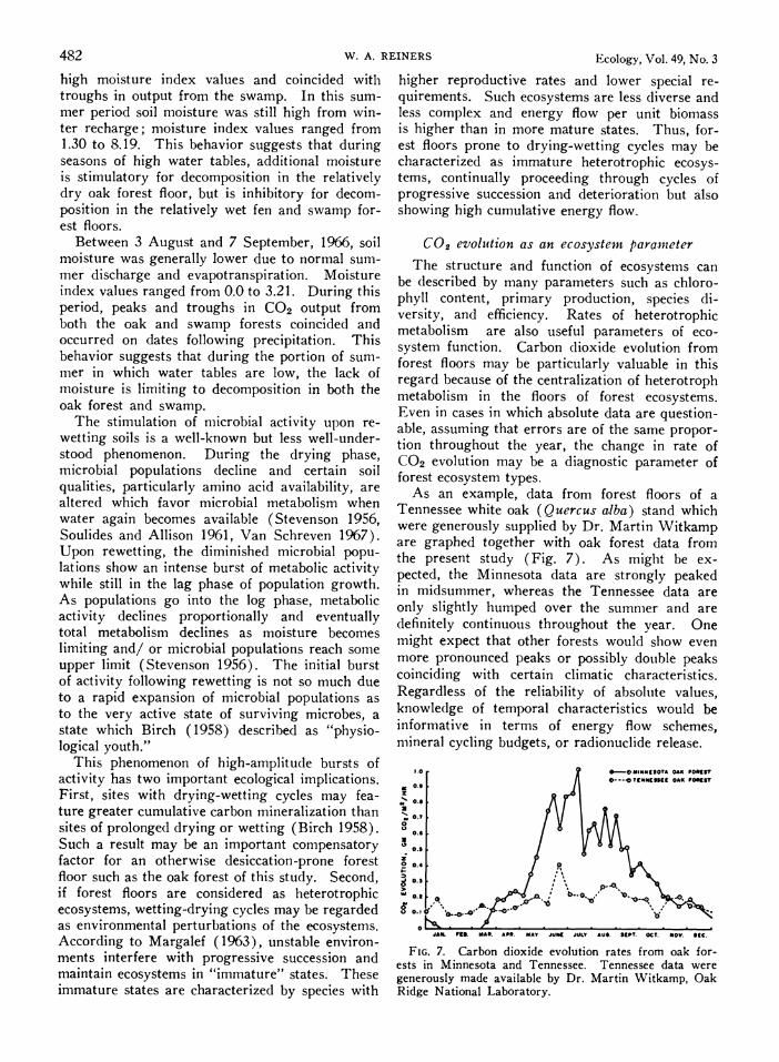
be described by many parameters such as chloro- phyll content, primary production, species di- versity, and efficiency. Rates of heterotrophic metabolism are also useful parameters of eco- system function. Carbon dioxide evolution from forest floors may be particularly valuable in this regard because of the centralization of heterotroph metabolism in the floors of forest ecosystems. Even in cases in which absolute data are question- able, assuming that errors are of the same propor- tion throughout the year, the change in rate of CO2 evolution may be a diagnostic parameter of forest ecosystem types.

As an example, data from forest floors of a Tennessee white oak (Quercus alba) stand which were generously supplied by Dr. Martin Witkamp are graphed together with oak forest data from the present study (Fig. 7). As might be ex- pected, the Minnesota data are strongly peaked in midsummer, whereas the Tennessee data are only slightly humped over the summer and are definitely continuous throughout the year. One might expect that other forests would show even more pronounced peaks or possibly double peaks coinciding with certain climatic characteristics. Regardless of the reliability of absolute values, knowledge of temporal characteristics would be informative in terms of energy flow schemes, mineral cycling budgets, or radionuclide release.

1.0 *-OMUIKKKOTA OAK F00137

O---Cet("9KSS OAK F0REST 0.3

O.K

K0.7

0.

20.

0O.3

0.6~~~~~~~~~~~-.

O.KA or -

0 JAW Fnd *AK. A0P. MAY JUKE JULY AU. SEPT. OCT. NOV. Sec.

FIG. 7. Carbon dioxide evolution rates from oak for- ests in Minnesota and Tennessee. Tennessee data were generously made available by Dr. Martin Witkamp, Oak Ridge National Laboratory.

Late Spring 1968 ENGELMANN SPRUCE IN COLORADO 483

ACKNOWLEDGMENTS

This study was supported by National Science Foun- dation grant GB-3636 and the Graduate School of the University of Minnesota. Thanks are due Dr. Eville Gorham for his helpful suggestions and Dr. William H. Marshall, Director of Cedar Creek Natural History Area, for his cooperation. Appreciation is extended to my wife, Norma, and Mr. Richard 0. Anderson for their aid in making field measurements. I am especially in- debted to Dr. Byron Brown and Mr. Siegfried Schach of the University of Minnesota Statistical Center for their invaluable assistance in statistical analysis of the data.

LITERATURE CITED

Ahlgren, Isabel F., and Clifford E. Ahlgren. 1965. Effects of prescribed burning on soil micro-organisms in a Minnesota jack pine forest. Ecology 46: 304- 310.

Birch, H. G. 1958. The effect of soil drying on humus decomposition and nitrogen availability. Plant and Soil 10: 9-31.

Birch, L. C., and D. P. Clarke. 1953. Forest soil as an ecological community with special reference to the fauna. Quart. Rev. Biol. 28: 13-36.

Bray, J. Roger. 1964. Primary consumption in three forest canopies. Ecology 45: 165-167.

Conway, Verona M. 1949. The bogs of central Min- nesota. Ecol. Monogr. 19: 173-206.

Daubenmire, R., and Don C. Prusso. 1963. Studies of the decomposition rates of tree litter. Ecology 44: 589-592.

Douglas, L. A., and J. C. F. Tedrow. 1959. Organic matter decomposition rates in arctic soils. Soil Sci. 88: 305-312.

Elkan, Gerald H., and W. E. C. Moore. 1962. A rapid method for measurement of CO2 evolution by soil microorganisms. Ecology 43: 775-776.

Fernald, M. L. 1950. Gray's manual of botany. 8th ed. American Book Company, New York. 1632 p.

Golley, Frank, Howard T. Odum, and Ronald F. Wil- son. 1962. The structure and metabolism of a Puerto Rican red mangrove forest in May. Ecology 43: 9-19.

Margalef, R. 1963. On certain unifying principles in ecology. Amer. Natur. 97: 357-374.

Olson, Jerry S. 1963. Energy storage and the balance of producers and decomposers in ecological systems. Ecology 44: 322-331.

Parr, J. F., and H. W. Reuszer. 1962. Organic matter decomposition as influenced by oxygen level and flow rate of gases in the constant aeration method. Soil Sci. Soc. Amer. Proc. 26: 552-556.

Romell, L. G. 1932. Mull and duff as biotic equilibria. Soil Sci. 34: 161-188.

Scheff6, Henry. 1959. The analysis of variance. John Wiley, New York. 477 p.

Soulides, D. A., and F. E. Allison. 1961. Effect of drying and freezing soils on carbon dioxide produc- tion, available mineral nutrients, aggregation, and bacterial population. Soil Sci. 91: 291-298.

Stevenson, I. J. 1956. Some observations on the mi- crobial-activity of remoistened air-dried soils. Plant and Soil 8: 170-182.

Thornthwaite, C. W. 1948. An approach toward a ra- tional classification of climate. Geogr. Rev. 38: 55- 94.

U.S. Department of Agriculture. 1941. Climate and man. Yearbook of Agriculture. U.S. Government Printing Office, Washington. 1248 p.

Van Schreven, D. A. 1967. The effect of intermittent drying and wetting of a calcareous soil on carbon and nitrogen mineralization. Plant and Soil 26: 14- 32.

Wallis, G. W., and S. A. Wilde. 1957. Rapid method for the determination of carbon dioxide evolved from forest soils. Ecology 38: 359-361.

Wiant, Harry V., Jr. 1967a. Contribution of roots to forest "soil respiration." Advancing Frontiers of Plant Sci. 18: 163-138.

. 1967b. Has the contribution of litter decay to forest "soil respiration" been overestimated? J. Forest. 65: 408-409.

. 1967c. Influence of temperature on the rate of soil respiration. J. Forest. 65: 489-490.

. 1967d. Influence of moisture content on "soil respiration." J. Forest. 65: 902-903.

Witkamp, Martin. 1966. Rates of carbon dioxide evolution from the forest floor. Ecology 47: 492- 494.

Witkamp, M., and J. Van der Drift. 1961. Break- down of forest litter in relation to environmental factors. Plant and Soil 15: 295-311.

ENGELMANN SPRUCE (PICEA ENGELMANNII ENGEL.) AT ITS UPPER LIMITS ON THE FRONT RANGE, COLORADO

PETER WARDLE Botany Division, Department of Scientific and Industrial Research

Christchurch, New Zealand (Accepted for publication February 20, 1968)

Abstract. Engelmann spruce is the dominant tree at timberline in the Front Range at approximately 3,350 m elevation; it occurs as krummholz in the forest-tundra ecotone up to about 3,500 m, and occasional individuals are found in the tundra up to 3,730 m. Tempera- tures decrease with increasing altitude above timberline, whereas wind velocity increases, especially during winter. Winter snow is deeper and persists longer in the forest than in the krummholz above, its depth in the latter tending to remain constant once the lower por- tions of the plants are packed. Soil temperatures fluctuate widely beneath tundra vegetation in the neighborhood of krummholz plants, whereas under forest variations are small and there is a prolonged period in spring when they remain within 0.60C (10F) of freezing point.