Carbon and NPP! - LEES Lab | MSUlees.geo.msu.edu/courses/geo827/lecture_9b_NPP.pdf · Carbon and...
58
Fall 2015 GEO 827 – Digital Image Processing and Analysis Carbon and NPP!
Transcript of Carbon and NPP! - LEES Lab | MSUlees.geo.msu.edu/courses/geo827/lecture_9b_NPP.pdf · Carbon and...
Fall 2015
GEO 827 – Digital Image Processing and Analysis
Carbon and NPP!

Fall 2015
GEO 827 – Digital Image Processing and Analysis
NPP and NEP
• Topics
– Respiration, production, and storage etc.
– Approaches
– How can remote sensing help?
– What has been done in this area?
– What are the limitations?
Fall 2015
GEO 827 – Digital Image Processing and Analysis
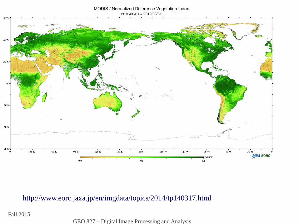
http://www.eorc.jaxa.jp/en/imgdata/topics/2014/tp140317.html
Fall 2015
GEO 827 – Digital Image Processing and Analysis
GPP
• Gross Primary Production denotes the total
amount of carbon fixed in the process of
photosynthesis by plants in an ecosystem,
such as a stand of trees.
• GPP is measured on photosynthetic tissues,
principally leaves. Global total GPP is
estimated to be about 120 Gt C yr-1.
Fall 2015
GEO 827 – Digital Image Processing and Analysis
NPP
• Net Primary Production denotes the net
production of organic matter by plants in an
ecosystem—that is, GPP reduced by losses
resulting from the respiration of the plants
(autotrophic respiration).
• Global NPP is estimated to be about half of
the GPP—that is, about 60 Gt C yr-1.

Fall 2015
GEO 827 – Digital Image Processing and Analysis
NEP• Net Ecosystem Production denotes the net accumulation of
organic matter or carbon by an ecosystem; NEP is the difference between the rate of production of living organic matter (NPP) and the decomposition rate of dead organic matter (heterotrophic respiration, RH).
• Heterotrophic respiration includes losses by herbivory and the decomposition of organic debris by soil biota. Global NEP is estimated to about 10 Gt C yr-1.
• NEP can be measured in two ways: One is to measure changes in carbon stocks in vegetation and soil; the other is to integrate the fluxes of CO2 into and out of the vegetation (the net ecosystem exchange, NEE) with instrumentation placed above (Aubinet et al., 2000).

Fall 2015
GEO 827 – Digital Image Processing and Analysis
NPP
• Global terrestrial carbon uptake. Plant (autotrophic) respiration releases CO2 to the atmosphere,
reducing GPP to NPP and resulting in short-term carbon uptake. Decomposition (heterotrophic
respiration) of litter and soils in excess of that resulting from disturbance further releases CO2 to the
atmosphere, reducing NPP to NEP and resulting in medium-term carbon uptake. Disturbance from both
natural and anthropogenic sources (e.g., harvest) leads to further release of CO2 to the atmosphere by
additional heterotrophic respiration and combustion—which, in turn, leads to long-term carbon storage
(adapted from Steffen et al., 1998).
Fall 2015
GEO 827 – Digital Image Processing and Analysis
NBP• Net Biome Production denotes the net production of organic matter
in a region containing a range of ecosystems (a biome) and includes,
in addition to heterotrophic respiration, other processes leading to
loss of living and dead organic matter (harvest, forest clearance, and
fire, etc.) (Schulze and Heimann, 1998).
• NBP is appropriate for the net carbon balance of large areas (100–
1000 km2) and longer periods of time (several years and longer). In
the past, NBP has been considered to be close to zero.
• Compared to the total fluxes between atmosphere and biosphere,
global NBP is comparatively small; NBP for the decade 1989–1998
has been estimated to be 0.7 ± 1.0 Gt C yr-1 (Table 1)-about 1
percent of NPP and about 10 percent of NEP.
Fall 2015
GEO 827 – Digital Image Processing and Analysis
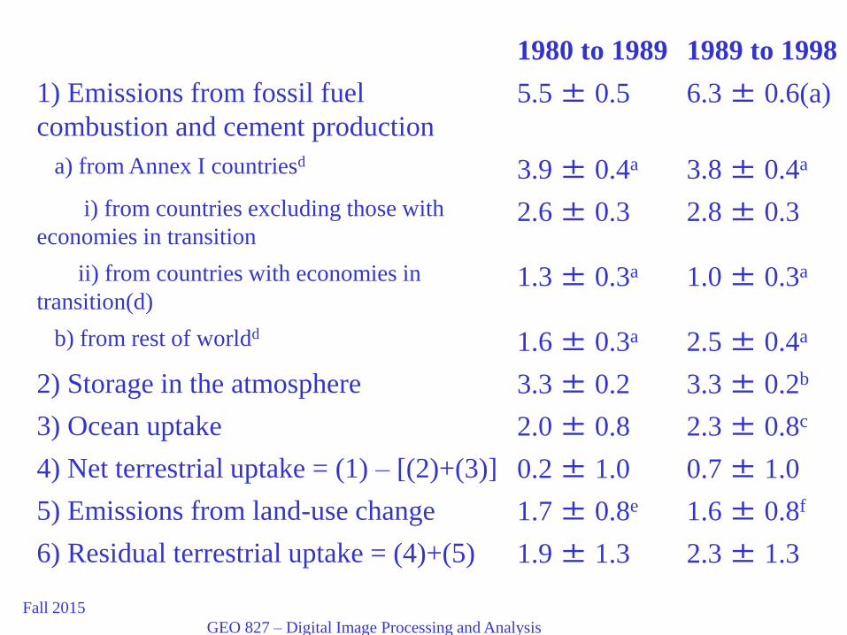
1980 to 1989 1989 to 1998
1) Emissions from fossil fuel
combustion and cement production
5.5 ± 0.5 6.3 ± 0.6(a)
a) from Annex I countriesd 3.9 ± 0.4a 3.8 ± 0.4a
i) from countries excluding those with
economies in transition2.6 ± 0.3 2.8 ± 0.3
ii) from countries with economies in
transition(d)1.3 ± 0.3a 1.0 ± 0.3a
b) from rest of worldd 1.6 ± 0.3a 2.5 ± 0.4a
2) Storage in the atmosphere 3.3 ± 0.2 3.3 ± 0.2b
3) Ocean uptake 2.0 ± 0.8 2.3 ± 0.8c
4) Net terrestrial uptake = (1) – [(2)+(3)] 0.2 ± 1.0 0.7 ± 1.0
5) Emissions from land-use change 1.7 ± 0.8e 1.6 ± 0.8f
6) Residual terrestrial uptake = (4)+(5) 1.9 ± 1.3 2.3 ± 1.3
Fall 2015
GEO 827 – Digital Image Processing and Analysis
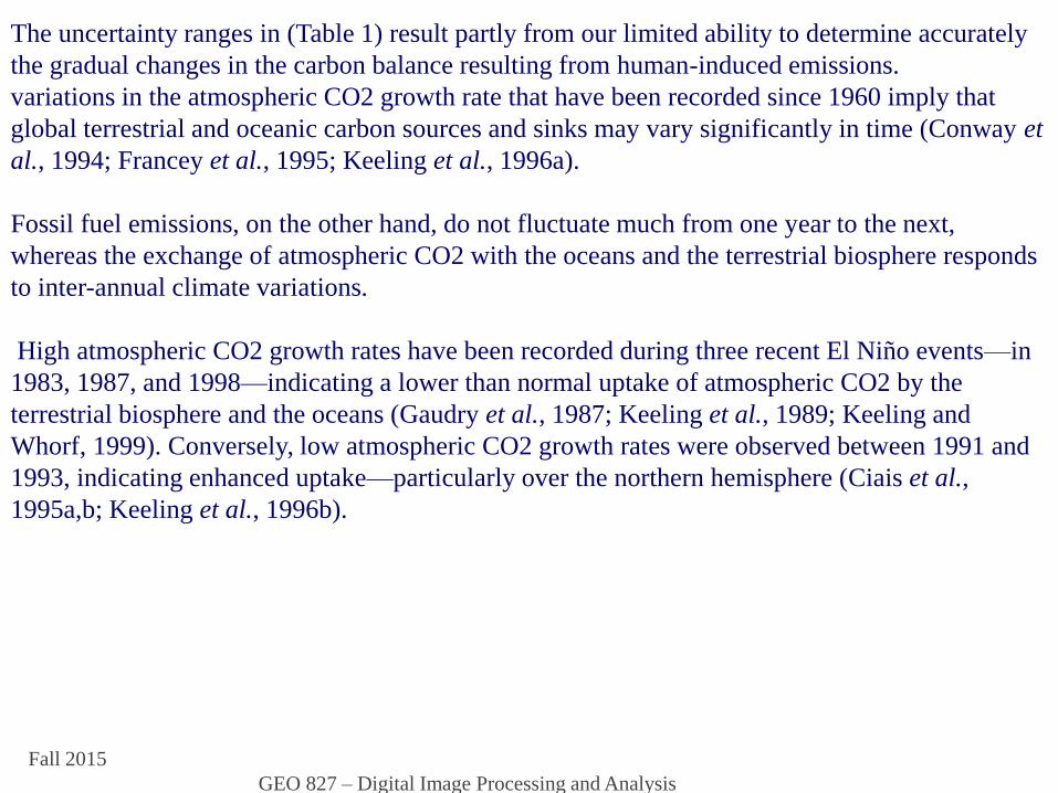
The uncertainty ranges in (Table 1) result partly from our limited ability to determine accurately
the gradual changes in the carbon balance resulting from human-induced emissions.
variations in the atmospheric CO2 growth rate that have been recorded since 1960 imply that
global terrestrial and oceanic carbon sources and sinks may vary significantly in time (Conway et
al., 1994; Francey et al., 1995; Keeling et al., 1996a).
Fossil fuel emissions, on the other hand, do not fluctuate much from one year to the next,
whereas the exchange of atmospheric CO2 with the oceans and the terrestrial biosphere responds
to inter-annual climate variations.
High atmospheric CO2 growth rates have been recorded during three recent El Niño events—in
1983, 1987, and 1998—indicating a lower than normal uptake of atmospheric CO2 by the
terrestrial biosphere and the oceans (Gaudry et al., 1987; Keeling et al., 1989; Keeling and
Whorf, 1999). Conversely, low atmospheric CO2 growth rates were observed between 1991 and
1993, indicating enhanced uptake—particularly over the northern hemisphere (Ciais et al.,
1995a,b; Keeling et al., 1996b).
Fall 2015
GEO 827 – Digital Image Processing and Analysis
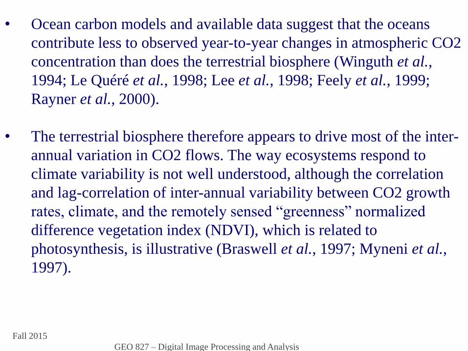
• Ocean carbon models and available data suggest that the oceans
contribute less to observed year-to-year changes in atmospheric CO2
concentration than does the terrestrial biosphere (Winguth et al.,
1994; Le Quéré et al., 1998; Lee et al., 1998; Feely et al., 1999;
Rayner et al., 2000).
• The terrestrial biosphere therefore appears to drive most of the inter-
annual variation in CO2 flows. The way ecosystems respond to
climate variability is not well understood, although the correlation
and lag-correlation of inter-annual variability between CO2 growth
rates, climate, and the remotely sensed “greenness” normalized
difference vegetation index (NDVI), which is related to
photosynthesis, is illustrative (Braswell et al., 1997; Myneni et al.,
1997).

Fall 2015
GEO 827 – Digital Image Processing and Analysis
• When terrestrial biogeochemical models are forced with realistic
year-to-year changes in temperature and precipitation, they can
simulate changes in the global and regional biosphere and associated
changes in CO2 exchange with the atmosphere (Kindermann et al.,
1996; Tian et al., 1998).
• These models can reproduce the magnitude and to some extent the
phase of observed inter-annual variability of atmospheric CO2
concentrations, though different processes have been implicated in
attempts to explain the observed fluctuations (e.g., Heimann et al.,
1997). There are still differences in detail that have not been
resolved.
Fall 2015
GEO 827 – Digital Image Processing and Analysis
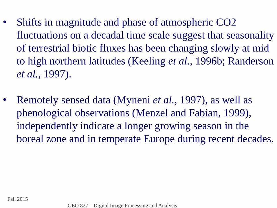
• Shifts in magnitude and phase of atmospheric CO2
fluctuations on a decadal time scale suggest that seasonality
of terrestrial biotic fluxes has been changing slowly at mid
to high northern latitudes (Keeling et al., 1996b; Randerson
et al., 1997).
• Remotely sensed data (Myneni et al., 1997), as well as
phenological observations (Menzel and Fabian, 1999),
independently indicate a longer growing season in the
boreal zone and in temperate Europe during recent decades.
Fall 2015
GEO 827 – Digital Image Processing and Analysis
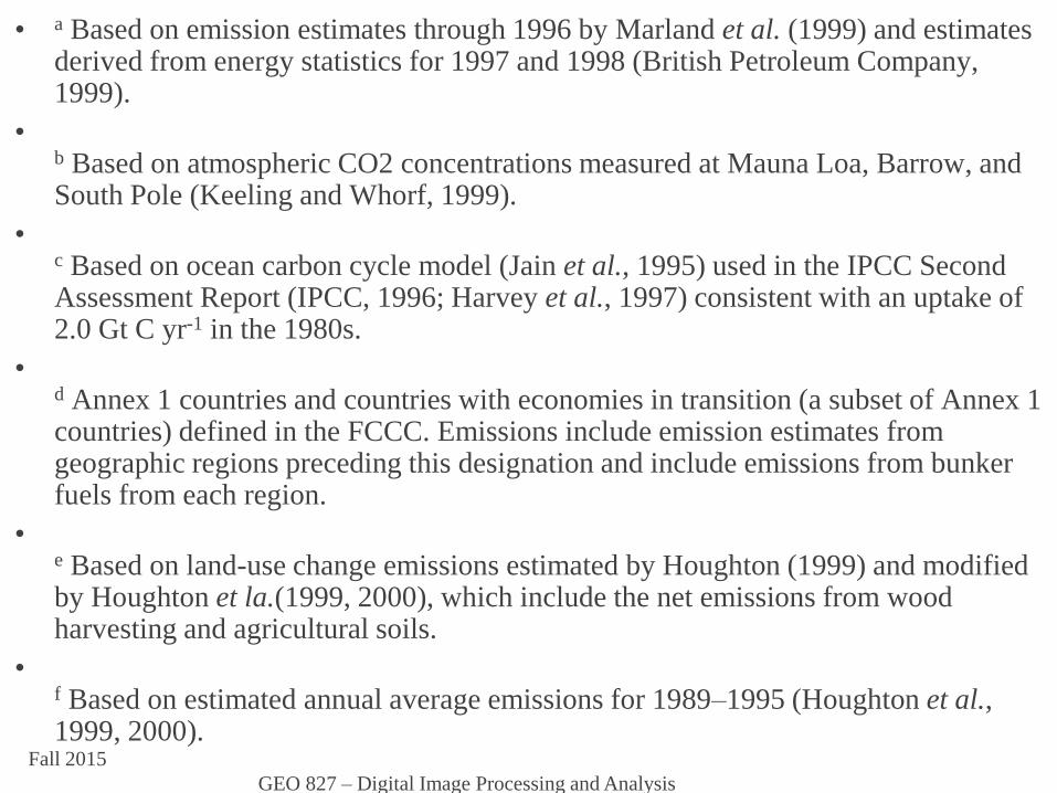
• a Based on emission estimates through 1996 by Marland et al. (1999) and estimates derived from energy statistics for 1997 and 1998 (British Petroleum Company, 1999).
•b Based on atmospheric CO2 concentrations measured at Mauna Loa, Barrow, and South Pole (Keeling and Whorf, 1999).
•c Based on ocean carbon cycle model (Jain et al., 1995) used in the IPCC Second Assessment Report (IPCC, 1996; Harvey et al., 1997) consistent with an uptake of 2.0 Gt C yr-1 in the 1980s.
•d Annex 1 countries and countries with economies in transition (a subset of Annex 1 countries) defined in the FCCC. Emissions include emission estimates from geographic regions preceding this designation and include emissions from bunker fuels from each region.
•e Based on land-use change emissions estimated by Houghton (1999) and modified by Houghton et la.(1999, 2000), which include the net emissions from wood harvesting and agricultural soils.
•f Based on estimated annual average emissions for 1989–1995 (Houghton et al., 1999, 2000).

(Daily) net photosynthesis (PSN)
and
(annual) net primary production
(NPP)
Fall 2015 GEO 827 – Digital Image
Processing and Analysis

Fall 2015
GEO 827 – Digital Image Processing and Analysis
PSN and NPP
(daily) net photosynthesis (PSN)
(annual) net primary production (NPP)
related to net carbon uptake
important for understanding global carbon budget
(climate change)
Increased CO2, climate change? Increased veg.
growth?
Fall 2015
GEO 827 – Digital Image Processing and Analysis
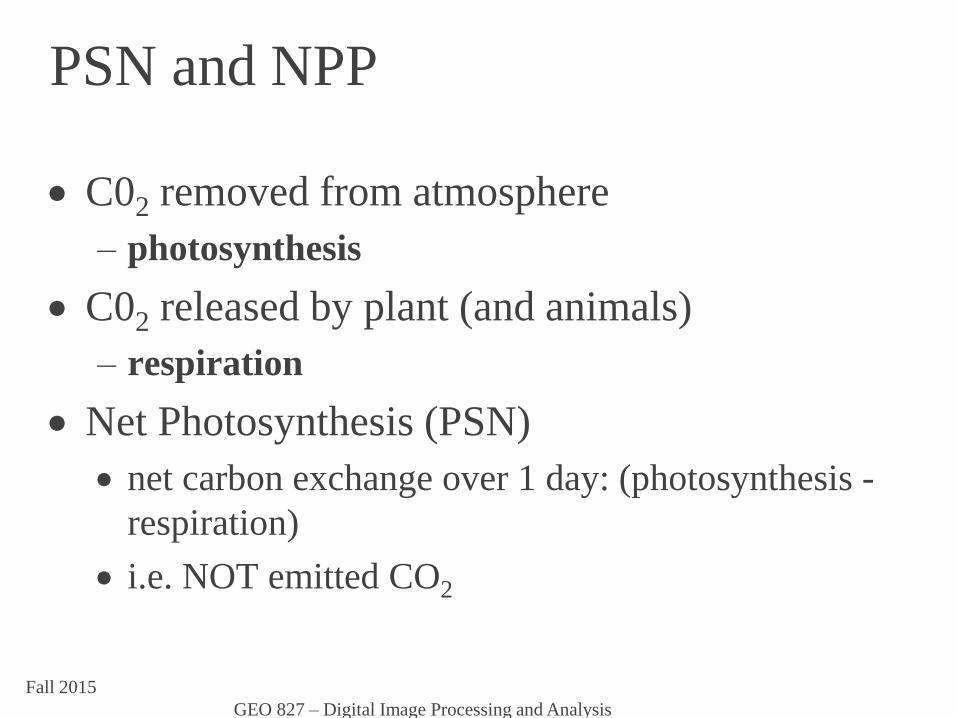
PSN and NPP
C02 removed from atmosphere
– photosynthesis
C02 released by plant (and animals)
– respiration
Net Photosynthesis (PSN)
net carbon exchange over 1 day: (photosynthesis -
respiration)
i.e. NOT emitted CO2
Fall 2015
GEO 827 – Digital Image Processing and Analysis
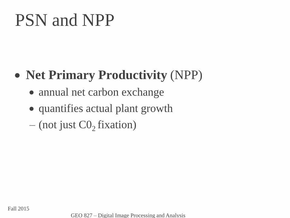
PSN and NPP
Net Primary Productivity (NPP)
annual net carbon exchange
quantifies actual plant growth
– (not just C02 fixation)
Fall 2015
GEO 827 – Digital Image Processing and Analysis
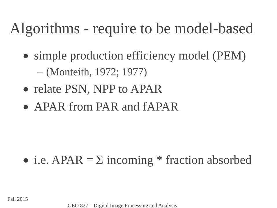
Algorithms - require to be model-based
simple production efficiency model (PEM)
– (Monteith, 1972; 1977)
relate PSN, NPP to APAR
APAR from PAR and fAPAR
i.e. APAR = incoming * fraction absorbed
APAR IPAR fAPAR
day
Fall 2015
GEO 827 – Digital Image Processing and Analysis
Extra reading
• http://nacarbon.org/nacp/documents/Our-
Changing-Planet_FY-2016_full%202.pdf
• https://downloads.globalchange.gov/strategic-
plan/2012/usgcrp-strategic-plan-2012.pdf
• https://carboncyclescience.us/state-carbon-cycle-
report-soccr
• http://nacarbon.org/nacp/documents.html?#ccs
• http://nacarbon.org/nacp/documents.html?#ccsp
• http://www.ntsg.umt.edu/
Fall 2015
GEO 827 – Digital Image Processing and Analysis
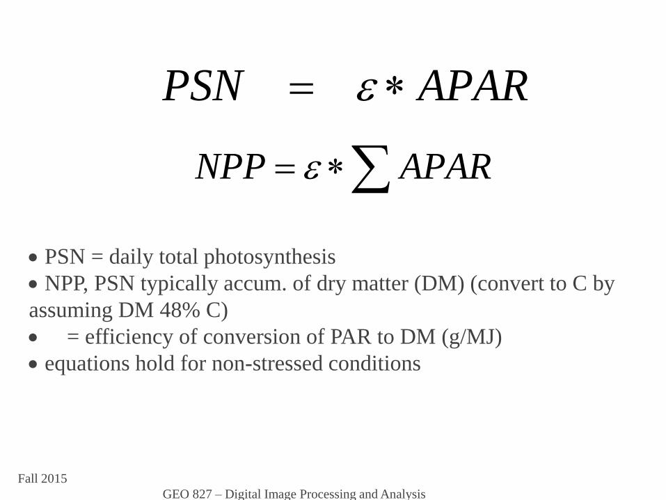
APARPSN
APARNPP
PSN = daily total photosynthesis
NPP, PSN typically accum. of dry matter (DM) (convert to C by
assuming DM 48% C)
= efficiency of conversion of PAR to DM (g/MJ)
equations hold for non-stressed conditions

Fall 2015
GEO 827 – Digital Image Processing and Analysis
To characterise vegetation need to know:
• Efficiency () and fAPAR
– But……..fAPAR NDVI
• So, for fixed
• So
• incident solar radiation (IPAR) also from RS
(Dubayah, 1992)
day
IPARPSN
)(
day
IPARNDVINPP

Fall 2015
GEO 827 – Digital Image Processing and Analysis
Determining
herbaceous vegetation (grasses):
av. 1.0-1.8 gC/MJ for C3 plants, higher for C4
woody vegetation:
0.2 - 1.5 gC/MJ
• simple model for :
mggross YYf
Fall 2015
GEO 827 – Digital Image Processing and Analysis
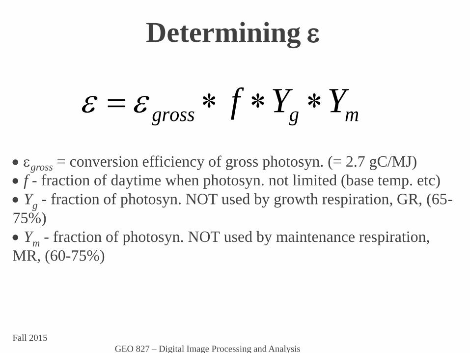
mggross YYf
gross = conversion efficiency of gross photosyn. (= 2.7 gC/MJ)
f - fraction of daytime when photosyn. not limited (base temp. etc)
Yg - fraction of photosyn. NOT used by growth respiration, GR, (65-
75%)
Ym - fraction of photosyn. NOT used by maintenance respiration,
MR, (60-75%)
Determining

Fall 2015
GEO 827 – Digital Image Processing and Analysis
define max - max. efficiency
max gross g mY Y
so f max
max - determined by plant form
f - determined by climate
base / max temperature
water or other stresses - light availability

Fall 2015
GEO 827 – Digital Image Processing and Analysis
Estimate max - land cover
LUT for biome characteristics
Estimate f - climatological inputs
can link to index of temperature/moisture
stress from surf. temp / VI
also require global Met. data (IPAR, rainfall)
Productivity algorithm

Fall 2015
GEO 827 – Digital Image Processing and Analysis
MODIS PSN/NPP algorithm
MODIS Product No. 17
Photosynthesis (PSN) 1km spatial, 8 day temporal resolution
Net Primary Productivity (NPP) 1km spatial, annual
Daily:
pixel-wise gross primary productivity terms computed and stored
8 day:
pixel-wise gross primary productivity terms computed and stored
8-day compositing routine - (8) contiguous daily products composited to
produce a single PSN or NPP 1KM global data product.
Annual:
annual NPP compositing routine 1KM global annual data product,
based on (365) day accumulated sum of GPP less maintenance respiration
(gpp - rm) term.

• Before 1980, biology focused at organismal level and ecological studies were carried out at 0.1 hectare field plots
• Lieth and Whittaker, 1975; produced a coarse global GPP map.
• When synoptic regional remote sensing began, field ecologists combined traditional measurements of plant biomass, primary productivity, canopy height and other ecological variables with satellite derived greenness to obtain the first global estimates of GPP.
Running et al
Introduction
Theory behind modeling GPP
1) plant NPP is directly related to absorbed solar energy
2) a connection exists between absorbed solar energy and satellite derived spectral indices of vegetation
3) assumption that there will be biophysical reasons why the absorbed light energy may be reduced below the theoretical
potential value.
Running et al

conceptual basis for modeling GPP
• Monteith’s light use efficiency (ε) is usually defined as the mass of carbon uptake per absorbed photosynthetically active radiation (APAR) from 400 nm to 700 nm wavelength.
• Gross primary production (GPP, g C m2 time-1) is summed over time periods ranging from instantaneous fluxes to annual totals
Running et al
Fall 2015
GEO 827 – Digital Image Processing and Analysis
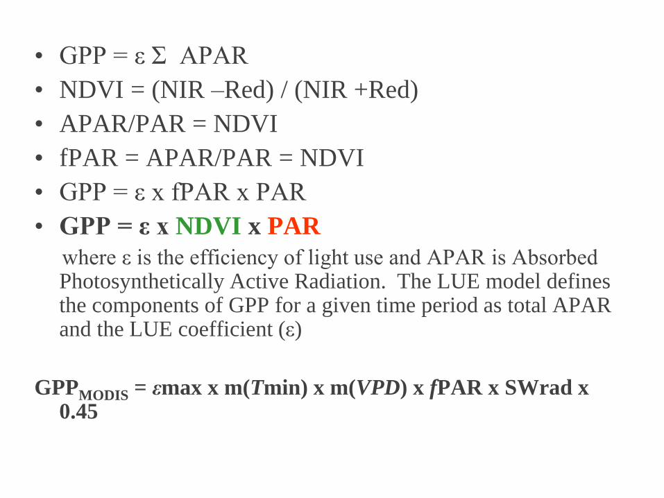
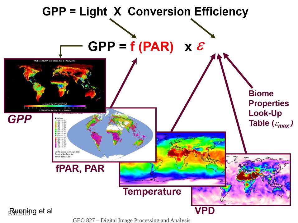
• GPP = ε Σ APAR
• NDVI = (NIR –Red) / (NIR +Red)
• APAR/PAR = NDVI
• fPAR = APAR/PAR = NDVI
• GPP = ε x fPAR x PAR
• GPP = ε x NDVI x PAR
where ε is the efficiency of light use and APAR is Absorbed Photosynthetically Active Radiation. The LUE model defines the components of GPP for a given time period as total APAR and the LUE coefficient (ε)
GPPMODIS = εmax x m(Tmin) x m(VPD) x fPAR x SWrad x 0.45
Running et al,
2002
Derivation of GPP Model

Running et al
2002
‘Big Foot’ scaling exercise
Running et al 2002

• VPM
• fPARcanopy = fPARchl + fPARNPV
• The VPM differs slightly from the MODIS GPP equation. Instead of the BPLUT look up table, derived from BIOME-BGC, εg is obtained from remote sensing and meteorological inputs as follows:
• GPP = εg x fPARchl x PAR where
εg = ε0 x Tscalar x Wscalar x Pscalar
where PAR is the photosynethically active radiation (μmol/m2/s, photosynthetic photon flux density), fPARchl is the fraction of PAR absorbed by chlorophyll, εg is the light use efficiency, LUE (μmol CO2/ μmol PAR).
• The parameter ε0 is the maximum light use efficiency (μmol CO2/ μmol PAR), and Tscalar, Wscalar, and Pscalar are the regulation scalars for the effects of temperature, water and leaf phenology on the light use efficiency of vegetation. On average, ε0 has a value around 1/6 for well-watered, C3 plants at optimal temperatures
Methods
Xiao et al ,
2004

Vegetation Indices
• Enhanced Vegetation Indices:
ρNIR, ρRed and ρBlue = atmospherically corrected surface reflectance
L = canopy background brightness correction factor (1)
C1 and C2 = atmospheric resistance Red and Blue correction coefficients (6&7.5)
G = Gain factor (2.5) - Huete et al., 2002
LCCGE
BluedNIR
dNIR
2Re1
Re -
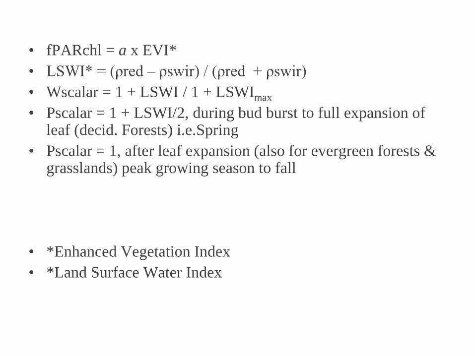
• fPARchl = a x EVI*
• LSWI* = (ρred – ρswir) / (ρred + ρswir)
• Wscalar = 1 + LSWI / 1 + LSWImax
• Pscalar = 1 + LSWI/2, during bud burst to full expansion of leaf (decid. Forests) i.e.Spring
• Pscalar = 1, after leaf expansion (also for evergreen forests & grasslands) peak growing season to fall
• *Enhanced Vegetation Index
• *Land Surface Water Index
Xiao et al ,
2004

• Tscalar is sensitivity of photosynthesis to temperature, calculated
at 8-day time step using an equation developed for the
Terrestrial Ecosystem Model*.
• Tscalar= (T- Tmin) (T- Tmax) / [(T- Tmin) (T- Tmax) - (T- Topt)2 ]
• where Tmin, Tmax, and Topt are minimum, maximum, and optimal
temperatures (˚C) for photosynthesis, respectively. If air
temperature falls below Tmin, Tscalar is set to zero
• Pscalar & Wscalar optimized for grasslands was changed to
reflect deciduous nature of Populus spp.and Artemisia ordosica
at K04 & 5
*Raich et al,
1991Xiao et al ,
2004

Modified Vegetation Photosynthesis Model (MVPM)
• Early LUE models assumed that LUE was constant; recent
studies have shown that LUE varies considerably across
ecosystem types and disturbance such as drought and diffuse
albedo
• Cascading error in estimating LUE LUT from coarse res. (1˚ x
1.25˚ pixel) DAO data
• studies suggested that independent measures of LUE were
unnecessary as they found good correlations between spectral
indices with carbon fluxes as well as with LUE
• much simpler from processing point of view to create a GPP
model entirely on remotely sensed data of similar resolution.
• it remains unclear as to what extent can short term variability in
carbon fluxes be estimated through spectral indices

• some scaling up studies in semi-arid areas using correlations between NDVI and carbon fluxes carried out but not across different ecosystem types
• VPM is not entirely independent of ground based sensor measurements such as PAR and temperature
• studied the feasibility of replacing these variables with MODIS derived GPP, fPAR and LST products
• GPP = α [ln (GPPMODIS) *(EVI*LSWI*LST)]/fPAR MODIS
• log-transferred GPPMODIS in the regression analysis because GPPtower may reflect only a fraction, possibly a nonlinear relationship with GPPMODIS which is an aggregate measure
over the 8-day period

Fall 2015
GEO 827 – Digital Image Processing and Analysis
MODIS PSN/NPP algorithm: stage 1
Basis is daily estimates of gross primary productivity, GPP -
using MOD15 FPAR product
For efficiency we need APAR – normally get fPAR from EO i.e.
APAR = PAR * fPAR
At-launch land-cover product radiation conversion efficiency
parameters from biome properties look-up table (BPLUT)
Fall 2015
GEO 827 – Digital Image Processing and Analysis
MODIS PSN/NPP algorithm: stage 1
Parameters in table estimated by multivariate
optimisation
minimise mean absolute error in daily GPP from MOD17
compared with separate Biome-BGC model.
This based on 1x1 simulations using Biome-BGC model,
met. data, 1km land cover product
Outputs include GPP, LAI and FPAR
Biome-BGC model
Predicts fluxes of water, carbon, nitrogen in a system including
vegetation, litter, soil, and near-surface atmosphere.
Fall 2015
GEO 827 – Digital Image Processing and Analysis
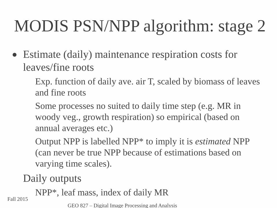
MODIS PSN/NPP algorithm: stage 2
Estimate (daily) maintenance respiration costs for
leaves/fine roots
Exp. function of daily ave. air T, scaled by biomass of leaves
and fine roots
Some processes no suited to daily time step (e.g. MR in
woody veg., growth respiration) so empirical (based on
annual averages etc.)
Output NPP is labelled NPP* to imply it is estimated NPP
(can never be true NPP because of estimations based on
varying time scales).
Daily outputs
NPP*, leaf mass, index of daily MR

Fall 2015
GEO 827 – Digital Image Processing and Analysis
MODIS PSN/NPP algorithm
Note inputs
required for GPP
assessment
Then require LAI
as well as other
ancillary data to
calc. MR –
Maintenance
Respiration
Fall 2015
GEO 827 – Digital Image Processing and Analysis
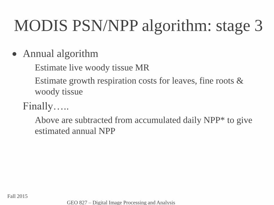
MODIS PSN/NPP algorithm: stage 3
Annual algorithm
Estimate live woody tissue MR
Estimate growth respiration costs for leaves, fine roots &
woody tissue
Finally…..
Above are subtracted from accumulated daily NPP* to give
estimated annual NPP

Fall 2015
GEO 827 – Digital Image Processing and Analysis
MODIS PSN/NPP algorithm

Fall 2015
GEO 827 – Digital Image Processing and Analysis
•Overview
•DAO – Data
Assimilation Office
Fall 2015
GEO 827 – Digital Image Processing and Analysis

Fall 2015
GEO 827 – Digital Image Processing and Analysis
Fall 2015
GEO 827 – Digital Image Processing and Analysis

Fall 2015
GEO 827 – Digital Image Processing and Analysis

Fall 2015
GEO 827 – Digital Image Processing and Analysis

Fall 2015
GEO 827 – Digital Image Processing and Analysis

Fall 2015
GEO 827 – Digital Image Processing and Analysis
Algorithm design: issues
• Instrument issues:
– spatial/spectral/temporal/angular resolution?
• Moderate (100m to km) - heterogeneity?
• High (<50m) – coverage?
– Cloud clearing, atmos. correction?
• Implementation issues
– Daily product?
• Rapid, near real-time processing
– Simple algorithm
– Size (storage, transfer)?
– Available ancillary data (PAR, LAI, NDVI, met. data etc.)

Fall 2015
GEO 827 – Digital Image Processing and Analysis
General algorithm design: BRDF/albedo
• Need samples of DHR and BHR
– Need V. good registration and atmos. correction
• directional effects easily masked
– Sample BRDF, model to interp./extrap.
• angular sampling crucial to accuracy
• Principle plane (PP) and XPP….
– Clouds reduce samples
– Magnitude inversion if < 3 samples
• Look-up veg. archetype BRDF from land-cover database
– Same (ish) shape, difference only in magnitude
• Associated error larger in this case
• Interp. between black-sky and white-sky to get
• Integral of narrow bands to broadband
Fall 2015
GEO 827 – Digital Image Processing and Analysis
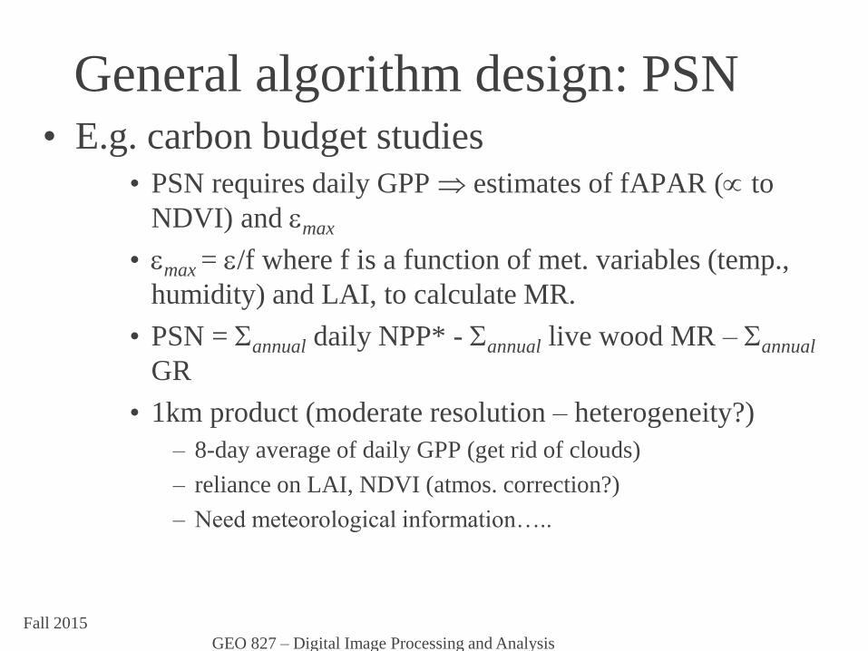
General algorithm design: PSN• E.g. carbon budget studies
• PSN requires daily GPP estimates of fAPAR ( to
NDVI) and max
• max = /f where f is a function of met. variables (temp.,
humidity) and LAI, to calculate MR.
• PSN = annual daily NPP* - annual live wood MR – annual
GR
• 1km product (moderate resolution – heterogeneity?)
– 8-day average of daily GPP (get rid of clouds)
– reliance on LAI, NDVI (atmos. correction?)
– Need meteorological information…..

Fall 2015
GEO 827 – Digital Image Processing and Analysis
Instrument considerations• wave/vis combined? e.g. ALOS, say (Japanese
– launch 2003)– AVNIR-2 (Adv. Vis. NIR Radiometer)
• 4 bands vis. NIR, 10m res. @ NADIR
• +/- 44°, steerable (combine with PALSAR)
– PALSAR (Phased array L-band SAR)
• 10m res., 70 km swath
– PRISM (Panchromatic Remote-sensing Instrument for Stereo
Mapping)
• For topo mapping but has angular signal (3 cameras)
• Combine to estimate land use, land cover,
change….BUT maybe biomass? Carbon?

Fall 2015
GEO 827 – Digital Image Processing and Analysis
• http://www.ipcc.ch/pub/tar/wg3/040.htm#810
• http://www.forestry.umt.edu/ntsg/RemoteSensing/netprimary/
• http://www.co2science.org/center.htm
• http://www.sciam.com/news/083101/2.html
• http://web.mit.edu/afs/athena.mit.edu/org/g/globalchange/www/rpt3.html
• ALOS: http://www.nasda.go.jp/Home/News/News-e/114eart.htm
• Dubayah, R. (1992) Estimating net solar radiation using Landsat Thematic Mapper and Digital Elevation data. Water resources Res., 28: 2469-2484.
• Monteith, J.L., (1972) Solar radiation and productivity in tropical ecosystems. J. Appl. Ecol, 9:747-766.
• Monteith, J.L., (1977). Climate and efficiency of crop production in Britain. Phil. Trans. Royal Soc. London, B 281:277-294.
• Running, S.W., Nemani, R., Glassy, J.M. (1996) MOD17 PSN/NPP Algorithm Theoretical Basis Document, NASA.
• Idso, K.E. and Idso, S.B. 1994. Plant responses to atmospheric CO2 enrichment in the face of environmental constraints: A review of the past 10 years' research, Agric. Forest Meteorol., 69:153-203.
PSN/NPP links/references