Capital Structure and Firm Performance: A New Approach to Testing Agency Theory and an Application to the Banking Industry

Allen N. Berger

Board of Governors of the Federal Reserve System Washington, DC 20551 U.S.A.

and Wharton Financial Institutions Center

Philadelphia, PA19104 U.S.A. aberger@frb.gov

Emilia Bonaccorsi di Patti Bank of Italy Rome, Italy

bonaccorsidipatti.emilia@insedia.interbusiness.it

Abstract

Corporate governance theory predicts that leverage affects agency costs and thereby influences firm performance. We propose a new approach to test this theory using profit efficiency, or how close a firm’s profits are to the benchmark of a best-practice firm facing the same exogenous conditions. We are also the first to employ a simultaneous-equations model that accounts for reverse causality from performance to capital structure. We also control for measures of ownership structure in the tests. We find that data on the U.S. banking industry are consistent with the theory, and the results are statistically significant, economically significant, and robust.

October 2002 JEL Codes: G32, G34, G21, G28. Keywords: Capital Structure, Agency Costs, Banking, Efficiency. The opinions expressed do not necessarily reflect those of the Board of Governors, the Bank of Italy, or their staffs. The authors thank Bob Avery, Hamid Mehran, George Pennacchi, Anjan Thakor, and other participants at the JFI/FRBNY/NYU Symposium on “Corporate Governance in the Banking and Financial Services Industries,” and seminar participants at the Federal Reserve Board for helpful comments, and Seth Bonime and Joe Scalise for valuable research assistance. Please address correspondence to Allen N. Berger, Mail Stop 153, Federal Reserve Board, 20th and C Streets. NW, Washington, DC 20551, call 202-452-2903, fax 202-452-5295, or email aberger@frb.gov.

1. Introduction

Agency costs represent important problems in corporate governance in both financial and nonfinancial

industries. The separation of ownership and control in a professionally managed firm may result in managers

exerting insufficient work effort, indulging in perquisites, choosing inputs or outputs that suit their own

preferences, or otherwise failing to maximize firm value. In effect, the agency costs of outside ownership equal

the lost value from professional managers maximizing their own utility, rather than the value of the firm.

Theory suggests that the choice of capital structure may help mitigate these agency costs. Under the

agency costs hypothesis, high leverage or a low equity/asset ratio reduces the agency costs of outside equity and

increases firm value by constraining or encouraging managers to act more in the interests of shareholders. Since

the seminal paper by Jensen and Meckling (1976), a vast literature on such agency-theoretic explanations of

capital structure has developed (see Harris and Raviv 1991 and Myers 2001 for reviews). Greater financial

leverage may affect managers and reduce agency costs through the threat of liquidation, which causes personal

losses to managers of salaries, reputation, perquisites, etc. (e.g., Grossman and Hart 1982, Williams 1987), and

through pressure to generate cash flow to pay interest expenses (e.g., Jensen 1986). Higher leverage can

mitigate conflicts between shareholders and managers concerning the choice of investment (e.g., Myers 1977),

the amount of risk to undertake (e.g., Jensen and Meckling 1976, Williams 1987), the conditions under which the

firm is liquidated (e.g., Harris and Raviv 1990), and dividend policy (e.g., Stulz 1990).

A testable prediction of this class of models is that increasing the leverage ratio should result in lower

agency costs of outside equity and improved firm performance, all else held equal. However, when leverage

becomes relatively high, further increases generate significant agency costs of outside debt – including higher

expected costs of bankruptcy or financial distress – arising from conflicts between bondholders and

shareholders.1 Because it is difficult to distinguish empirically between the two sources of agency costs, we

follow the literature and allow the relationship between total agency costs and leverage to be nonmonotonic.

Despite the importance of this theory, there is at best mixed empirical evidence in the extant literature

(see Harris and Raviv 1991, Titman 2000, and Myers 2001 for reviews). Tests of the agency costs hypothesis

typically regress measures of firm performance on the equity capital ratio or other indicator of leverage plus

some control variables. At least three problems appear in the prior studies that we address in our application.

1 In the case of the banking industry studied here, there are also regulatory costs associated with very high leverage.

2

First, the measures of firm performance are usually ratios fashioned from financial statements or stock

market prices, such as industry-adjusted operating margins or stock market returns. These measures do not net

out the effects of differences in exogenous market factors that affect firm value, but are beyond management’s

control and therefore cannot reflect agency costs. Thus, the tests may be confounded by factors that are

unrelated to agency costs. As well, these studies generally do not set a separate benchmark for each firm’s

performance that would be realized if agency costs were minimized.

We address the measurement problem by using profit efficiency as our indicator of firm performance.

The link between productive efficiency and agency costs was first suggested by Stigler (1976), and profit

efficiency represents a refinement of the efficiency concept developed since that time.2 Profit efficiency

evaluates how close a firm is to earning the profit that a best-practice firm would earn facing the same

exogenous conditions. This has the benefit of controlling for factors outside the control of management that are

not part of agency costs. In contrast, comparisons of standard financial ratios, stock market returns, and similar

measures typically do not control for these exogenous factors. Even when the measures used in the literature are

industry adjusted, they may not account for important differences across firms within an industry – such as local

market conditions – as we are able to do with profit efficiency. In addition, the performance of a best-practice

firm under the same exogenous conditions is a reasonable benchmark for how the firm would be expected to

perform if agency costs were minimized.

Second, the prior research generally does not take into account the possibility of reverse causation from

performance to capital structure. If firm performance affects the choice of capital structure, then failure to take

this reverse causality into account may result in simultaneous-equations bias. That is, regressions of firm

performance on a measure of leverage may confound the effects of capital structure on performance with the

effects of performance on capital structure.

We address this problem by allowing for reverse causality from performance to capital structure. We

discuss below two hypotheses for why firm performance may affect the choice of capital structure, the

efficiency-risk hypothesis and the franchise-value hypothesis. We construct a two-equation structural model and

estimate it using two-stage least squares (2SLS). An equation specifying profit efficiency as a function of the

2 Stigler’s argument was part of a broader exchange over whether productive efficiency (or X-efficiency) primarily reflects difficulties in reconciling the preferences of multiple optimizing agents – what is today called agency costs – versus “true” inefficiency, or failure to optimize (e.g., Stigler 1976, Leibenstein 1978).

3

firm’s equity capital ratio and other variables is used to test the agency costs hypothesis, and an equation

specifying the equity capital ratio as a function of the firm’s profit efficiency and other variables is used to test

the net effects of the efficiency-risk and franchise-value hypotheses. Both equations are econometrically

identified through exclusion restrictions that are consistent with the theories.

Third, some, but not all of the prior studies did not take ownership structure into account. Under

virtually any theory of agency costs, ownership structure is important, since it is the separation of ownership and

control that creates agency costs (e.g., Barnea, Haugen, and Senbet 1985). Greater insider shares may reduce

agency costs, although the effect may be reversed at very high levels of insider holdings (e.g., Morck, Shleifer,

and Vishny 1988). As well, outside block ownership or institutional holdings tend to mitigate agency costs by

creating a relatively efficient monitor of the managers (e.g., Shleifer and Vishny 1986). Exclusion of the

ownership variables may bias the test results because the ownership variables may be correlated with the

dependent variable in the agency cost equation (performance) and with the key exogenous variable (leverage)

through the reverse causality hypotheses noted above.

To address this third problem, we include ownership structure variables in the agency cost equation

explaining profit efficiency. We include insider ownership, outside block holdings, and institutional holdings.

Our application to data from the banking industry is advantageous because of the abundance of quality

data available on firms in this industry. In particular, we have detailed financial data for a large number of firms

producing comparable products with similar technologies, and information on market prices and other

exogenous conditions in the local markets in which they operate. In addition, some studies in this literature find

evidence of the link between the efficiency of firms and variables that are recognized to affect agency costs,

including leverage and ownership structure (see Berger and Mester 1997 for a review).

Although banking is a regulated industry, banks are subject to the same type of agency costs and other

influences on behavior as other industries. The banks in the sample are subject to essentially equal regulatory

constraints, and we focus on differences across banks, not between banks and other firms. Most banks are well

above the regulatory capital minimums, and our results are based primarily on differences at the margin, rather

than the effects of regulation. Our test of the agency costs hypothesis using data from one industry may be built

upon to test a number of corporate finance hypotheses using information on virtually any industry.

4

The paper is organized as follows. Section 2 discusses issues of measuring performance, reverse

causality, and the use of ownership structure in tests of the agency costs of capital structure. Section 3 specifies

the simultaneous equations model for testing the hypotheses, and Section 4 describes the data and variables

employed in the model. Section 5 describes the empirical results, and Section 6 concludes. Appendix A details

the efficiency estimation.

2. Measures of Performance, Reverse Causality, and the Use of Ownership Structure

In this section, we show in greater detail how we address the three main problems in testing the agency

costs hypothesis. We discuss the choice of performance measure (subsection 2.1), give the theories of reverse

causality from performance to capital structure (subsection 2.2), and describe the use of ownership structure

variables in the empirical model (subsection 2.3).

2.1. Measures of firm performance

The literature employs a number of different measures of firm performance to test agency cost

hypotheses. These measures include 1) financial ratios from balance sheet and income statements (e.g., Demsetz

and Lehn 1985, Gorton and Rosen 1995, Mehran 1995, Ang, Cole, and Lin 2000), 2) stock market returns and

their volatility (e.g., Saunders, Strock, and Travlos 1990, Cole and Mehran 1998), and 3) Tobin’s q, which mixes

market values with accounting values (e.g., Morck, Shleifer, and Vishny 1988, McConnell and Servaes 1990,

1995, Mehran 1995, Himmelberg, Hubbard, and Palia 1999, Zhou 2001).3

We argue that profit efficiency – i.e., frontier efficiency computed using a profit function – is a more

appropriate measure to test agency cost theory because it controls for the effects of local market prices and other

exogenous factors and because it provides a reasonable benchmark for each individual firm’s performance if

agency costs were minimized.4 Profit efficiency is superior to cost efficiency for evaluating the performance of

managers, since it accounts for how well managers raise revenues as well as control costs and is closer to the

concept of value maximization.5 Although maximizing accounting profits and maximizing shareholder value are

not identical, it seems reasonable to assume that shareholder losses from agency costs are close to proportional to

3 Other studies of agency problems use different methodologies. For example, one study of agency costs estimates the effect of debt on input misallocation using elasticities derived from a cost function (Kim and Maksimovic 1991). Some studies of expense preference behavior use input demand functions (e.g., Hannan and Mavinga 1980, Mester 1989). 4 Frontier efficiency is sometimes called X-efficiency or managerial efficiency. 5 The only study that uses profit efficiency in a similar context is DeYoung, Spong, and Sullivan (2001), who analyze the effect of managerial ownership on the performance of a sample of small, closely held banks. However, they test only the effects of managerial ownership and do not include capital structure or test the agency costs hypothesis.

5

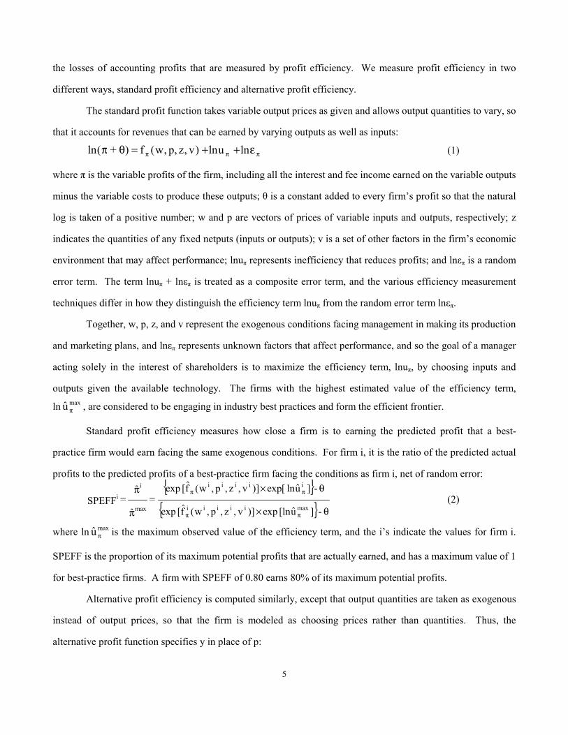
the losses of accounting profits that are measured by profit efficiency. We measure profit efficiency in two

different ways, standard profit efficiency and alternative profit efficiency.

The standard profit function takes variable output prices as given and allows output quantities to vary, so

that it accounts for revenues that can be earned by varying outputs as well as inputs:

πππ ε++=θπ lnuln)v,z,p,w(f ) + (ln (1)

where π is the variable profits of the firm, including all the interest and fee income earned on the variable outputs

minus the variable costs to produce these outputs; θ is a constant added to every firm’s profit so that the natural

log is taken of a positive number; w and p are vectors of prices of variable inputs and outputs, respectively; z

indicates the quantities of any fixed netputs (inputs or outputs); v is a set of other factors in the firm’s economic

environment that may affect performance; lnuπ represents inefficiency that reduces profits; and lnεπ is a random

error term. The term lnuπ + lnεπ is treated as a composite error term, and the various efficiency measurement

techniques differ in how they distinguish the efficiency term lnuπ from the random error term lnεπ.

Together, w, p, z, and v represent the exogenous conditions facing management in making its production

and marketing plans, and lnεπ represents unknown factors that affect performance, and so the goal of a manager

acting solely in the interest of shareholders is to maximize the efficiency term, lnuπ, by choosing inputs and

outputs given the available technology. The firms with the highest estimated value of the efficiency term,

ln maxu π , are considered to be engaging in industry best practices and form the efficient frontier.

Standard profit efficiency measures how close a firm is to earning the predicted profit that a best-

practice firm would earn facing the same exogenous conditions. For firm i, it is the ratio of the predicted actual

profits to the predicted profits of a best-practice firm facing the conditions as firm i, net of random error: { }

{ } θ×

θ×

π

π

ππ

ππ

- ]u[ln exp )]v,z,p,w(f[ exp

- ]uln [exp)]v,z,p,w(f[ exp =

ˆ

ˆ = SPEFF

maxiiiii

iiiii

max

i

i (2)

where ln maxu π is the maximum observed value of the efficiency term, and the i’s indicate the values for firm i.

SPEFF is the proportion of its maximum potential profits that are actually earned, and has a maximum value of 1

for best-practice firms. A firm with SPEFF of 0.80 earns 80% of its maximum potential profits.

Alternative profit efficiency is computed similarly, except that output quantities are taken as exogenous

instead of output prices, so that the firm is modeled as choosing prices rather than quantities. Thus, the

alternative profit function specifies y in place of p:

6

πππ ε++=θπ lnln)v,z,y,w(f ) + (ln u (3)

The efficiency scores are calculated in the same way as the standard profit measures except for this change in the

arguments of the profit function:

{ }

{ } θ×

θ×

π

π

ππ

ππ

- ]u[ln exp )]v,z,y,w(f[ exp

- ]uln [exp)]v,z,y,w(f[ exp =

ˆa

ˆa = APEFF

maxa

iiiiia

ia

iiiia

max

i

i (4)

The concept of alternative profit may be helpful when some of the assumptions underlying the cost and standard

profit functions are not met.6

We consider profit efficiency to be a reasonable (inverse) proxy for the agency costs due to managers

pursuing their own objectives rather than maximizing shareholder value. The predicted profit of a best-practice

firm under the same exogenous conditions as firm i is an individual firm benchmark that the owners of firm i

might reasonably ask their managers to try to achieve. It does not assume zero agency costs or define a purely

technological best practice, but it takes into account how well firms in the industry actually perform and the

exogenous conditions under which the firm operates. The value of the firm is the present value of expected

future profits, so the deviation from the profits that the industry’s best management would achieve should be

reasonably close to proportional to shareholder losses from agency costs. We argue that netting out the effects

on profits of exogenous factors beyond the control of management is important to measuring agency costs of

managers pursuing their own objectives. We also argue that the observed behavior of the best-practice firms is

about as close as an approximation as possible to how a firm would behave if agency costs were minimized.

As noted, tests of the agency cost effects of capital structure in the literature generally use financial

ratios and/or stock market values to measure performance. Such variables do not remove the effects of

differences in exogenous factors that affect firm value and which may be confounded with agency costs in the

tests. The prior studies also generally do not set a separate benchmark for each firm’s performance that would

be realized if agency costs were minimized. This may be especially difficult for studies using market price and

return data, which are based upon expectations and performance relative to expectations, rather than

performance relative to a minimum-agency cost benchmark.7

6 Alternative profit efficiency has been shown to help when i) there are substantial unmeasured differences in the quality of banking services; ii) outputs are not completely variable; iii) output markets are not perfectly competitive; and/or iv) output prices are not accurately measured (see Berger and Mester 1997). 7 One study analyzing small firms Ang, Cole, and Lin (2000) set as the benchmarks for analyzing small firms the financial

7

2.2. Theories of reverse causality from performance to capital structure

As noted, prior research on agency costs generally does not take into account the possibility of reverse

causation from performance to capital structure, which may result in simultaneous-equations bias. We offer two

hypotheses of reverse causation based on violations of the Modigliani-Miller perfect-markets assumption. It is

assumed that various market imperfections (e.g., taxes, bankruptcy costs, asymmetric information) result in a

balance between those favoring more versus less equity capital, and that differences in profit efficiency move the

optimal equity capital ratio marginally up or down.8

Under the efficiency-risk hypothesis, more efficient firms choose lower equity ratios than other firms, all

else equal, because higher efficiency reduces the expected costs of bankruptcy and financial distress. Under this

hypothesis, higher profit efficiency generates a higher expected return for a given capital structure, and the

higher efficiency substitutes to some degree for equity capital in protecting the firm against future crises. This is

a joint hypothesis that i) profit efficiency is strongly positively associated with expected returns, and ii) the

higher expected returns from high efficiency are substituted for equity capital to manage risks.

The evidence is consistent with the first part of the hypothesis, i.e., that profit efficiency is strongly

positively associated with expected returns in banking. Profit efficiency has been found to be significantly

positively correlated with returns on equity and returns on assets (e.g., Berger and Mester 1997) and other

evidence suggests that profit efficiency is relatively stable over time (e.g., DeYoung 1997), so that a finding of

high current profit efficiency tends to yield high future expected returns.

The second part of the hypothesis – that higher expected returns for more efficient banks are substituted

for equity capital – follows from a standard Altman z-score analysis of firm insolvency (Altman 1968). High

expected returns and high equity capital ratio can each serve as a buffer against portfolio risks to reduce the

probabilities of incurring the costs of financial distress/bankruptcy, so firms with high expected returns owing to

high profit efficiency can hold lower equity ratios. The z-score is the number of standard deviations below the

expected return that the actual return can go before equity is depleted and the firm is insolvent, zi = (µi +

ECAPi)/σi, where µi and σi are the mean and standard deviation, respectively, of the rate of return on assets, and

ratios for those that were fully owned by a single owner-manager. This may be an improvement in the analysis of agency costs for small firms, but it does not address our main issues of controlling for differences in exogenous conditions and in setting up individualized firm benchmarks for performance. 8 See Harris and Raviv (1991) and Myers (2001) for general discussions of the choice of capital structure, and see Berger, Herring, and Szegö (1995) for a discussion that focuses on capital choices in banking.

8

ECAPi is the ratio of equity to assets. Based on the first part of the efficiency-risk hypothesis, firms with higher

efficiency will have higher µi. Based on the second part of the hypothesis, a higher µi allows the firm to have a

lower ECAPi for a given z-score, so that more efficient firms may choose lower equity capital ratios.

The franchise-value hypothesis focuses on the income effect of the economic rents generated by profit

efficiency on the choice of leverage. Under this hypothesis, more efficient firms choose higher equity capital

ratios, all else equal, to protect the rents or franchise value associated with high efficiency from the possibility of

liquidation. Higher profit efficiency may create economic rents if the efficiency is expected to continue in the

future, and shareholders may choose to hold extra equity capital to protect these rents, which would be lost in the

event of liquidation, even if the liquidation involves no overt bankruptcy or distress costs.

Prior evidence supports the notion that firms hold additional equity capital to protect franchise value.

For example, the relaxation of chartering rules the early 1980s appears to have resulted in banks lowering their

equity capital and taking on more portfolio risk, since they had less franchise value to protect (e.g., Keeley

1990). Firms with unique products are also found to have higher equity capital ratios, all else equal, as product

uniqueness can create market power rents and the firm may hold extra equity capital to protect these rents (e.g.,

Titman 1984, Titman and Wessels 1988). In banking, it is often argued that relationship lending creates such

rents because the bank has proprietary access to information about loan customers (e.g., Petersen and Rajan

1995). The franchise-value hypothesis is a joint hypothesis that profit efficiency is a source of rents, and that

banks hold additional equity capital to prevent the loss of these rents in the event of liquidation.

These two hypotheses yield opposite predictions from one another for the effects of profit efficiency on

equity capital or leverage. The two individual effects may be thought of as substitution and income effects.

Under the efficiency-risk hypothesis, the expected earnings from high profit efficiency substitute for equity

capital in protecting the firm from the expected costs of bankruptcy or financial distress, whereas under the

franchise-value hypothesis, firms try to protect the income from high profit efficiency by holding additional

equity capital. We interpret the findings below as the net effect of these two hypotheses, or whether the

substitution versus income effects dominate. Thus, these hypotheses are only partially identifiable in the sense

that we can only distinguish which one is more important than the other.

2.3. The use of ownership structure variables

9

We argue that ownership structure as well as capital structure should be included in studies of agency

costs, since it is the separation of ownership and control that creates the agency costs. A number of prior studies

examine the effects of capital structure on performance without controlling for ownership structure (e.g. Titman

and Wessels 1988), while others evaluated the effects of ownership structure on performance without controlling

for capital structure (e.g. Mester 1993, Pi and Timme 1993, Gorton and Rosen 1995, DeYoung, Spong and

Sullivan 2001). Finally, other research does include both variables but considers leverage as exogenous, rather

than using a simultaneous equations framework (e.g., Mehran 1995, McConnell and Servaes 1995).

The exclusion of ownership structure variables may bias tests of the agency costs hypothesis of the

effects of capital structure on firm performance. Any excluded ownership variables are expected to be correlated

with the performance dependent variable and with the included capital structure variable (equity capital ratio)

through the reverse causality from performance to capital structure discussed earlier. We include variables on

the composition of shareholdings and on the holding company structure in the agency cost equation explaining

profit efficiency in our analysis below. In addition to solving some potential bias problems, the effects of these

variables on firm performance are interesting on their own.

3. The Empirical Model

We test the agency costs hypothesis that increasing leverage or decreasing the equity/asset ratio is

associated with a reduction in the agency costs of outside equity and an improvement in firm performance by

regressing profit efficiency on the equity capital ratio plus control variables. The regression equation may be

written as:

EFFi = f1 (ECAPi, Z1i) + e1i , (5)

where EFFi is a measure of firm i’s standard or alternative profit efficiency, and ECAPi is the ratio of equity

capital to gross total assets. The use of ECAPi as an inverse measure of leverage is standard in banking research

in part because of the regulatory attention paid to capital ratios. The vector Z1i contains other characteristics that

are likely to influence profit efficiency, including measures of ownership structure, market concentration, firm

size, variance of earnings, and the regulatory environment. Finally, e1i is a mean-zero disturbance term. All of

the variables are measured over the period 1990-1995, and in most cases are averages over this period.

The agency costs hypothesis predicts that an increase in leverage raises efficiency, i.e., ∂EFF/∂ECAP <

0, as higher equity capital ratios or lower leverage reduce pressure on managers from outside equity holders to

10

maximize value, aggravating agency problems between these parties and owners and reducing profit efficiency.

We test this hypothesis against the null of ∂EFF/∂ECAP = 0. However, when leverage is sufficiently high,

further increases may result in lower efficiency because the benefits in terms of reduced agency costs of outside

equity are overcome by greater agency costs of debt. We specify a quadratic functional form that includes

ECAP and ½ECAP2 to allow the relationship between agency costs and leverage to be nonmonotonic and

reverse signs when leverage is high. Importantly, we are testing the joint hypothesis that leverage affects agency

costs and that profit inefficiency embodies at least some of these agency costs.

The efficiency-risk and franchise-value hypotheses are tested using the parameters of the second

equation in the model, which determines the equity capital ratio as a function of profit efficiency:

ECAPi = f2 (EFFi, Z2i) + e2i (6)

The vector Z2i contains factors other than profit efficiency that are likely to influence the equity capital

ratio, including measures of local market prices, firm size, variance of earnings, market concentration, and the

regulatory environment. The error term e2i may be correlated with the error term from equation (5), e1i. The two-

equation model is econometrically identified by exclusion restrictions in the Z vectors (discussed below), and is

estimated by two-stage least squares (2SLS).

The efficiency-risk hypothesis predicts that firms with high profit efficiency will substitute out of equity

capital, so that ∂ECAP/∂EFF < 0 in equation (6). In contrast, the franchise-value hypothesis predicts that firms

with high profit efficiency will try to protect the value of their high income by holding more equity capital, so

that ∂ECAP/∂EFF > 0. It is likely that each hypothesis describes the equity choices of a subset of banks. We

interpret the estimated derivative as the net effect of these two hypotheses, or an indicator of whether the

substitution effect versus the income effect generally dominates. We again specify a quadratic form, including

both EFF and ½EFF2 to allow the reverse causality to be nonmonotonic.

4. The Data and Variables

To implement our tests, we use annual information on U.S. commercial banks from 1990 through 1995,

taken mostly from the Reports of Income and Condition (Call Reports). We include only banks in existence for

all six years. We use averages for each bank over these years in order to reduce the effects of temporary shocks

on the measurement of efficiency and to examine the equilibrium relationships in the data. For our main

hypothesis tests, we employ our “ownership sample” of 695 banks for which detailed information on the insider,

11

outside block, and institutional holdings of the bank (or its top-tier holding company) is available from the SEC

Filings and taken from Compact Disclosure. We exclude banks that changed top tier holding company in the

period to avoid problems created by ownership changes. To ensure robustness, we also run the model and test

the hypotheses using our “full sample” of 7320 banks – all U.S. banks that were in continuous existence over

1990-1995, whether or not all the ownership variables are available (excluding those that changed top tier

holding company). For both samples, we use efficiency estimates derived from the full sample, so that firm

efficiency is appropriately measured against a frontier based on the best practice banks in the industry, whether

or not they have ownership data available. Table 1 shows the variables employed in the model, their definitions,

and summary statistics for both samples.

4.1. The dependent variables, EFF and ECAP

Our performance measures are standard profit efficiency, SPEFF, which takes output prices to be

exogenous, and alternative profit efficiency, APEFF, which takes output quantities to be exogenous. The

efficiency measures are computed using the distribution-free method, under which we estimate profit functions

(1) and (3) for each year in our 1990-1995 panel, allowing the estimated parameters to vary over time. The

functions are estimated using the Fourier-flexible functional form, which has been shown to fit the data for U.S.

banks better than the conventional translog form. The efficiency measures in equations (2) and (4) are computed

from the six-year averages of the estimated residual terms (lnu + lnε) based on the assumption that the core

efficiency terms lnu remain constant for each bank over time, and the random errors lnε to tend to average out

over time. See Appendix A for more details. As a robustness check, we also employ efficiencies estimated

using a fixed-effects method based on a dummy variable for each bank instead of the average residual. The

suffixes “_DF” and “_FE” designate the efficiencies measured using the distribution-free and fixed-effects

methods, respectively. Our (inverse) measure of leverage is ECAP, the book value of equity capital to gross

total assets.

4.2. The exogenous variables in the efficiency equation (5)

The vector of control variables in the efficiency equation (5), Z1, includes measures of ownership

structure, other bank characteristics, market factors, and regulation. The ownership structure variables include

three measures of the composition of shareholdings of the top-tier holding company – insider shareholdings by

board members and relatives (SHINSIDE), shareholdings owned by outsiders with more than 5% of the

12

outstanding shares (SH_5OWN), and the share of institutional holdings (SHINSTIT). Greater insider shares are

usually expected to reduce agency costs, but there is also evidence of managerial entrenchment for high levels of

insider holdings (e.g., Morck, Shleifer, and Vishny 1988, McConnell and Servaes 1990,1995, Gorton and Rosen

1995). To allow for potential nonmonotonicity, we include first-, second- and third-order terms in the insider

share, SHINSIDE, ¹⁄2SHINSIDE2, and ¹⁄6SHINSIDE3. A positive effect of SH_5OWN is expected if outside

block owners are able to help mitigate problems of controlling managers. Large block shareholdings may also

improve the effectiveness of the takeover mechanism by mitigating the free rider problem (e.g., Shleifer and

Vishny 1986). Finally, SHINSTIT is expected to have a positive coefficient if institutional investors monitor the

managers more closely than other shareholders (McConnell and Servaes 1995).

We also include variables describing the bank’s holding company structure: whether the holding

company is multi-layered (MULTILAY) and whether the top-tier holding company is located out of state

(OUTSTATE). In the full sample, we add a dummy variable equal to 1 if the bank is in a bank holding company

(INBHC), 0 otherwise (all banks in the ownership sample are also in holding companies). Greater organizational

complexity may be associated with lower efficiency to the extent that it makes control more difficult, and may

be associated with greater efficiency to the extent that it improves diversification and investment opportunities.

We also control for bank risk. Riskier banks may be measured as more profit efficient on average if they

are trading off between risk and expected return. This may occur if risky banks “skimp” on loan monitoring,

saving monitoring costs, but having more variable returns on their loan portfolios (Berger and DeYoung 1997).

Alternatively, banks that are poor at operations might also be poor at risk management, yielding a negative

relationship between profit efficiency and risk. We include SDROE, the standard deviation of ROE over the six-

year period for each bank, as well as a second-order term, ¹⁄2SDROE2, to allow for nonmontonicity. To control

for differences associated with bank size, we include size class dummy variables (SIZE1 through SIZE7). These

variables help account for the effects of differences in technology, investment opportunities, diversification, and

other factors related to size (SIZE1 is excluded as the base case).

Finally, market and regulatory factors are specified as follows. As a proxy for market power, we include

the weighted-average Herfindahl index (HERF) of local deposit market concentration for the bank, where

weights are the proportions of the bank's deposits in all its markets (Metropolitan Statistical Areas or rural

counties). Differences in regulatory environment are accounted for by dummy variables for operation in a

13

limited branching state (LIMITB) or in a unit banking state (UNITB), with operation in a statewide branching

state (STATEB) as the excluded category.

4.3. The exogenous variables in the capital equation (6)

The vector of control variables in the capital equation (6), Z2, includes market prices, other bank

characteristics, and market and regulatory factors. We include market prices as determinants of ECAP because

prices directly affect profitability (negatively for input prices, positively for output prices), and because our two

hypotheses underlying the ECAP equation are based on equity being a substitute for expected profits versus

being used to protect expected profits. The prices are calculated as exogenous market averages that a bank faces

in its local market(s).9 These prices incorporate supply and demand conditions for assets and liabilities in the

markets in which the bank operates, and include potential rents from market power of the banks in these markets.

We include the prices of the three variable inputs, purchased funds (MW1), labor (MW2), and core deposits

(MW3), and the four variable outputs, consumer loans (MP1), business loans (MP2), real estate loans (MP3),

and securities (MP4) that were employed in the estimation of standard profit efficiency.

The variables describing other bank characteristics are the same risk and size variables included in

equation (5). As a relevant market factor, we include concentration as a proxy for market power. The original

version of the franchise-value hypothesis was stated in terms of rents associated with market power (rather than

efficiency), so we include HERF to control for market power that is not already fully captured by the prices. The

regulatory variables are again the dummies UNITB and LIMITB, with STATEB as the excluded category.

4.4. Identification of the model

The two-equation simultaneous-equations model is econometrically identified because there are properly

specified variables in each of the Z vectors that are appropriately excluded from the other. Measures of

ownership structure (SHINSIDE, SH5OWN, SHINSTIT, MULTILAY, OUTSTATE, INBHC) affect efficiency

and are included in Z1. These variables are excluded from Z2, because these factors should affect capital only

through efficiency or risk, both of which are already controlled for in equation (6). When we employ the

ownership sample, the variable INBHC is not available since all banks in the ownership sample are in bank

holding companies. When we employ the full sample, the variables SHINSIDE, SH5OWN, and SHINSTIT are

9 The price of each variable input or output faced by the bank is the weighted average of the prices of the other banks in the market excluding the bank’s own price, where the weights are each other bank’s share of the total of that input or output of all the other banks in the market. A bank’s price is then the weighted average of the prices it faces in each of its markets, where the weight is the share of the bank’s deposits in its branches in that market.

14

available for only the ownership subsample, so we set these variables to zero for the other banks and add a

dummy variable OWNERSAMPLE to flag the ownership sample. In either case, there are more than enough

instruments available for identification. We assume that the choice of capital ratio is not itself subject to

manipulation by managers since owners can observe it, so that ownership structure should not directly affect the

choice of capital ratio. Put another way, the ownership variables are assumed not to affect ECAP directly in

equation (6), since there is no reason to expect market forces to require more or less equity capital based on

ownership structure except to the extent that the ownership structure affects the firm’s efficiency or risk.10,11

The market prices faced for inputs and outputs (MW1, MW2, MW3, MP1, MP2, MP3, MP4) affect

equity capital and are included in Z2. All seven of these prices are properly excluded from Z1 when standard

profit efficiency (SPEFF) is specified, since the calculation of standard profit efficiency takes both input and

output prices as given and maximizes profits. That is, SPEFF measures how well the firm behaves after taking

local market input and output prices and other business conditions into account. When alternative profit

efficiency (APEFF) is specified, the model is identified by the exclusion of the three input prices only, because

calculation of alternative profit efficiency takes input prices as given, but allows output prices to vary. For the

alternative profit efficiency model, we also tried adding the four output prices to Z1, so that the model would not

be falsely identified by the exclusion of these variables, and found that the results were materially unchanged

(not shown in tables).12 Equation (5) would not generally be identified using conventional measures of

performance, such as financial ratios or stock market prices, since these variables are directly affected by all

input and output prices.

5. Results

In this section, we show our main results and robustness checks for the hypothesis tests. For

expositional convenience, we first discuss all of the tests and robustness checks for the agency costs hypothesis,

using equation (5) to test the effects of the equity capital ratio on efficiency. We then review the findings for 10 In our empirical application, a number of the ownership structure measures are statistically significant in all of the first-stage regressions of SPEFF and APEFF on the exogenous variables, supporting the identification of equation (6). 11 Some studies find that ownership structure affects leverage, although the specification is much different from ours (e.g., Mehran 1992, Mehran, Taggart and Yermack 1999). If there is a direct causation from ownership structure to capital, our exclusion of the ownership variables from equation (6) would affect the coefficients for this equation but would not bias the coefficients of equation (5), which is our main tool for testing the agency costs hypothesis, the hypothesis of primary interest here. For robustness purposes, we also estimated the model including ownership structure variables in equation (6) and our results for equation (5) did not change significantly. 12 At least two of the input prices are statistically significant in all of the first-stage regressions of ECAP on the prices and other exogenous variables, supporting the identification of equation (5).

15

reverse causality from efficiency to equity capital using equation (6) to test between the effects of the efficiency-

risk and franchise-value hypotheses.

5.1. Tests of the agency costs hypothesis using equation (5)

Table 2 presents our main results. We show estimates of equation (5) and (6) by 2SLS for the ownership

sample, using both standard and alternative profit efficiency calculated using the distribution-free efficiency

method (SPEFF_DF and APEFF_DF).13 For both efficiency measures, the coefficient of ECAP in equation (5)

is negative and statistically significant and the coefficient of ½ECAP2 is positive but not statistically significant.

For testing the agency costs hypothesis, we evaluate the derivative of efficiency with respect to ECAP at the

value ECAP = .082, the sample mean for the ownership sample. As shown near the bottom of Table 2,

∂EFF/∂ECAP takes on the values of -6.063 and -4.888 and is statistically significant at the 1% level in both

cases, consistent with the agency costs hypothesis.14 However, the data are not consistent with the prediction

that agency costs of outside debt may reverse the relationship at very high leverage (low ECAP), perhaps due to

constraints imposed by regulators.

The estimated magnitudes of ∂EFF/∂ECAP are also economically significant. In the standard profit

efficiency model (SPEFF_DF) estimated by 2SLS (Table 2, column 1), a decrease in the equity capital ratio of 1

percentage point increases profit efficiency by about 6 percentage points. For a bank at the mean equity ratio of

8.2% and the mean profit efficiency of 54%, an exogenous decrease in ECAP by one percentage point to 7.2% is

predicted to raise SPEFF_DF to about 60%, or an increase in actual profits of more than 10% (.06/.54). The

2SLS results for the alternative profit efficiency model (APEFF_DF) yields a similar effect (.05/.53).15

Figure 1 maps out the predicted levels of profit efficiency SPEFF_DF and APEFF_DF for various levels

of ECAP, holding all the other variables at the sample mean. For both efficiency measures, ∂EFF/∂ECAP is

negative for all values of ECAP up to about 0.16 to 0.17. These findings are again consistent with the agency

13 Because the endogenous variables enter the regression with a nonlinear functional form, we estimate the model following Kelejian (1971), who shows that the 2SLS estimator based on the Taylor series approximation for the reduced forms using linear terms and higher powers of the exogenous variables are consistent. In particular, we obtain the predicted values by regressing ECAP and ½ECAP2 on quadratic terms and cross products of the exogenous variables at the first stage (we exclude higher order terms and cross-terms between dummy variables). The same procedure is used to obtain the predicted values of EFF and ½EFF2 in the first stage in estimating equation (6). 14 The derivative ∂EFF/∂ECAP at the mean is given by β1 + β2 * .082, where β1 is the coefficient of ECAP and β2 is the coefficient of ½ECAP2. 15 We also estimated a log specification for ECAP in equation (5) and found consistent results (not shown).

16

costs hypothesis for virtually all large, professionally managed banks, which generally have equity capital well

below these levels.

Turning to the other variables in equation (5), the effect of SHINSIDE is nonlinear because of the first-,

second-, and third-order terms. Although not very significant, the coefficients in column 1 suggest a slight

improvement in performance as insider shares increase within the moderate range of about 16% to 60% insider

holdings, as predicted by agency cost models. However, it also shows a slight negative derivative at very low

levels of insider ownership below about 16% and a negative derivative at very high levels of such ownership

above about 60%. This relationship is similar to that found in the literature cited above.

The variable for outside block ownership, SH5OWN, has a negative sign and is moderately statistically

significant in both regressions. This finding suggests that an increase in outside block ownership reduces profit

efficiency, which is not consistent with the hypothesis of increased monitoring incentives from more

concentrated outside ownership.16 However, institutional holdings, SHINSTIT, appear to have a strong positive

effect on profit efficiency, consistent with the predictions of favorable effects from institutional owners. These

coefficients together are consistent with the possibility that large institutional holders have favorable monitoring

effects, whereas large individual investors do not.

The negative coefficients of MULTILAY suggest that banks in multi-layered holding companies are less

profit efficient, consistent with problems created by organizational complexity. Banks with holding companies

headquartered out of state are not significantly different in terms of profit efficiency from those with an in-state

holding company.

The SIZE dummy variables have negative and significant coefficients, suggesting that larger banks tend

to be less efficient, everything else equal. The coefficients for the first- and second-order terms in SDROE are

conflicting, suggesting that the effects of risk may be nonmonotonic. At the sample mean, the effect of SDROE

on efficiency is negative (-0.9). Market concentration as measured by HERF appears to have a positive effect on

profit efficiency. This is consistent with earlier research that found that higher concentration may lead to lower

cost efficiency but higher profit efficiency, as increased net revenues from exploitation of market power in

pricing are partially offset by that increased costs from managers pursuing other objectives (Berger and Mester

1997, Berger and Hannan 1998). Finally, banks that have been allowed statewide branching are more profit

16 Previous evidence is also not consistent with the hypothesis that large block shareholders take an active monitoring role (e.g., McConnell and Servaes 1990).

17

efficient than those where branching is limited. The effects of unit banking are not statistically significant, likely

because only a few banks are in unit banking states at the start of the sample period.

Table 3 shows estimates for equation (5) based on different specifications to test for robustness, again

using the ownership sample. In the first two columns, we estimate (5) using OLS instead of 2SLS. The main

results are robust to the estimation method using both measures of efficiency (SPEFF and APEFF). The OLS

estimates of ∂EFF/∂ECAP are again statistically significant and economically significant. An exogenous

decrease in ECAP by one percentage point at the sample mean implies an increase in actual profits of about 6%

to 8% (i.e., .03/.54 to .04/.54).

In the last two columns of Table 3, we replace EFF in equation (5) with the bank’s return on equity

(ROE), a conventional measure of performance. Since the input and output prices directly affect returns we show

in column 4 a modified specification in which we add the input and output prices to the regressor list. The ROE

equations are estimated by OLS and are not fully identified because these prices cannot be used as instruments as

they directly affect ROE. Once again, the results are consistent with the agency costs hypothesis and statistically

and economically significant. An exogenous decrease in ECAP by one percentage point at the sample mean

implies an increase in ROE of about 6% from the mean ROE of 12.1% (i.e., .0075/.121).17

To ensure robustness, we switch from the distribution-free method to the fixed-effects method of

estimating efficiency. The regressions shown in Table 4 replicate the main regressions from Table 2 except for

the use of this different method of measuring efficiency. Under this method, we include a dummy variable for

every bank in the profit functions and use the coefficients of these dummies in place of the average error terms

for each bank from the profit functions used in the distribution-free method.18 The main results concerning the

effects of equity capital are robust with respect to this change in methodology both for the standard profit

17 In previous research, the effect of ECAP on ROE was found to vary from positive to negative, depending on the time period (e.g., Berger 1995). 18 The distribution-free method employed in our main results forces orthogonality between the main component of the efficiency measure (the average error term for the bank) and a (nonlinear) function of the equity capital ratio, since equity is included in the profit functions. Similarly, orthogonality is imposed between the main component of the efficiency and a nonlinear function of the prices of variable inputs and outputs that are used to identify equation (5), potentially affecting the identification of the model. The fixed-effects method does not force any orthogonality of the efficiencies with these other variables. However, we prefer the distribution-free method because of other problems with the fixed-effects method. Prior research found that the fixed effects were confounded by the differences in scale, which are several thousand times larger in magnitude than differences in efficiency in typical banking data sets (Berger 1993). As shown in Table 1, measured efficiencies using the fixed-effects method are quite low. For example, the mean standard profit efficiency using the fixed-effects methodology is 11.3%. We consider it to be unrealistic that the average bank earns only 11.3% of the profits that a best-practice bank facing the same conditions would earn.

18

(SPEFF_FE) and the alternative profit (APEFF_FE) measures. The derivative of efficiency with respect to

ECAP is statistically significant in both the standard and alternative profit efficiency models. In the standard

profit efficiency model in the first column, a decrease in the equity capital ratio of 1 percentage point increases

profit efficiency by about 2 percentage points. For a bank at the mean equity ratio of 8.2% and the mean profit

efficiency of 16%, an exogenous decrease in ECAP by one percentage point to 7.2% is predicted to raise

SPEFF_FE to about 18%, or an increase in actual profits of more than 12% (.02/.16). The results for the

alternative profit efficiency model (APEFF_FE) yield a larger effect (.04/.19).

Table 5 shows an additional robustness check in which we re-estimate the model for the full sample of

banks, i.e., include banks with no data on public ownership. This provides a greater variety in terms of bank

size, capitalization, and ownership structure. However, it also presents a problem in that many of these

additional banks are owner managed rather than professionally managed, and therefore do not provide a good

laboratory for testing the agency costs of the separation of ownership and management.19 Nonetheless, the

results for equation (5) in the first two columns of Table 5 are again consistent with the agency costs hypothesis.

The effect of ECAP on efficiency, ∂EFF/∂ECAP, is negative, statistically and economically significant, and

similar in magnitude to that obtained in our main regression.

As a final robustness check, we re-estimated the model employing data for the period 1984-1989 in

place of 1990-1995. The results were very similar results both in terms of coefficient magnitudes and

significance. The derivative of efficiency with respect to ECAP from equation (5) is negative and statistically

significant in both the standard and alternative profit efficiency models also for the 1980s. In both cases, the

magnitude of the effect of ECAP on efficiency is larger for the 1980s than for the 1990s data. In particular, in

the standard profit efficiency model the derivative at the sample mean is -10.041, implying that a decrease in the

equity capital ratio of 1 percentage point increases profit efficiency by about 10 percentage points. For a bank at

the mean equity ratio of 6.8% and the mean profit efficiency of 66%, an exogenous decrease in ECAP by one

percentage point to 5.8% is predicted to raise SPEFF_DF to about 76%, or an increase in actual profits of about

15% (.10/.66). The derivative of efficiency with respect to ECAP for the alternative profit efficiency model

(APEFF_FE) is equal to -8.85, implying a slightly smaller effect (.08/.65).

19 The data on shareholdings are available only for the ownership sample used in the main tests, which is a subsample here, so we include in equation (5) the variable OWNERSAMPLE that is equal to one if SHINSIDE, SH_5OWN, SHINSTIT are available and zero otherwise, flagging these observations to account for their average difference from other banks.

19

5.2. Tests of the efficiency-risk and franchise-value hypotheses using equation (6)

We next turn to our results from testing reverse causality from efficiency to equity capital, i.e., using

equation (6) to test between the effects of the efficiency-risk and franchise-value hypotheses. The main findings

for the ownership sample are reported in the last two columns of Table 2. We do not find strong dominance of

one hypothesis over the other. We evaluate the derivative of ECAP with respect to efficiency at the ownership

sample mean of value SPEFF_DF = .543 or APEFF_DF = .532. As shown near the bottom of Table 2, the

estimates of ∂ECAP/∂EFF are negative and statistically significant at the mean, supporting the efficiency-risk

hypothesis over the franchise-value hypothesis.

However, this finding does not hold for all the relevant values of efficiency. Figure 2 maps out the

predicted levels of ECAP for various levels of profit efficiency SPEFF_DF and APEFF_DF, holding all the

other variables at the sample mean. For both efficiency measures, ∂ECAP/∂EFF is positive for all values of EFF

up to about 0.40, and then negative thereafter. Thus, for low relatively levels of profit efficiency, the findings

are consistent with a dominance of the efficiency-risk hypothesis, under which the expected additional earnings

from higher efficiency substitute for equity capital in protecting the firm from the expected costs of bankruptcy

or financial distress. For relatively high levels of efficiency, in contrast, the findings are more consistent with a

dominance of the franchise-value hypothesis, under which firms try to protect the higher expected income from

higher efficiency by holding additional equity capital.

With respect to the control variables in equation (6), all of the prices except for two (MW1 and MW3)

are not statistically significant. The SIZE variables are all significant with negative coefficients, consistent with

the conventional wisdom that larger banks are better diversified and can thus hold less capital to buffer against

losses. However, the effect of SDROE at the sample mean is statistically significant and negative (-0.04). The

coefficient of HERF is positive and statistically significant, consistent with the influence of expected future rents

from local market power on the capital structure decision.

The regressions shown in the last two columns of Table 4 replicate the regressions in the last two

columns of Table 2 except for the use of the efficiencies measured by the fixed-effects method rather than with

the distribution-free method. We evaluate the derivative of ECAP with respect to efficiency at the ownership

sample mean of value SPEFF_FE = .159 or APEFF_FE = .191. As shown near the bottom of Table 2, the

estimates of ∂ECAP/∂EFF are negative at the mean, although the derivative is not statistically significant for the

20

SPEFF_FE model. The first-order terms in EFF are positive and second-order terms are negative, so that the

derivative again changes sign, but the shape of the curve with ECAP as a function of EFF (not shown) would be

convex or inverted from the curve shown in Figure 2 above. Again, the results suggest that neither the

efficiency-risk hypothesis nor the franchise-value hypothesis dominates the other.

In contrast, the full sample results for equation (6) shown in the last two columns of Table 5 are

consistent with a strong, consistent dominance of the efficiency-risk hypothesis over the franchise-value

hypothesis. The estimated derivatives ∂ECAP/∂EFF are negative and statistically significant at all values of

efficiency and are much larger than in the ownership sample. These findings are also economically significant.

The derivative of efficiency is about -0.12 using both efficiency measures. In the SPEFF_DF model, an increase

in efficiency of 10 percentage points from the mean – from 0.58 to 0.68 – implies a reduction in ECAP of 1.2

percentage points – from 9.4% to 8.2% – or a reduction of about 13% (.012/.094). Thus, for the full sample,

banks with higher efficiency tend to substitute out of equity capital. This suggests a difference in behavior for

the small banks that comprise most of the full sample. These banks may substitute more in part because their

capital ratios tend to be higher than those of the large banks that make up the bulk of the ownership sample.

Finally, the results for equation (6) using the ownership sample data from the 1980s shown in the last

two columns of Table 6 suggest a negative value for ∂ECAP/∂EFF at the sample mean, consistent with a

dominance of the efficiency-risk hypothesis over the franchise-value hypothesis. However, the effect is

relatively small and similar to the findings for the ownership sample using the 1990s data in Tables 2 and 4.

6. Conclusions

We test the agency costs hypothesis of corporate finance, under which high leverage reduces the agency

costs of outside equity and increases firm value by constraining or encouraging managers to act more in the

interests of shareholders. Our use of profit efficiency as an indicator of firm performance to measure agency

costs, our specification of a two-equation structural model that takes into account reverse causality from firm

performance to capital structure, and our inclusion of measures of ownership structure address problems in the

extant empirical literature that may help explain why prior empirical results have been mixed. Our application to

the banking industry is advantageous because of the detailed data available on a large number of comparable

firms and the exogenous conditions in their local markets. Although banks are regulated, we focus on

differences across banks that are driven by corporate governance issues, rather than any differences in

21

regulation, given that all banks are subject to essentially the same regulatory framework and most banks are well

above the regulatory capital minimums.

Our findings are consistent with the agency costs hypothesis – higher leverage or a lower equity capital

ratio is associated with higher profit efficiency, all else equal. The effect is economically significant as well as

statistically significant. An increase in leverage as represented by a 1 percentage point decrease in the equity

capital ratio yields a predicted increase in profit efficiency of about 6 percentage points, or a gain of about 10%

in actual profits at the sample mean. This result is robust to a number of specification changes, including

different measures of performance (standard profit efficiency, alternative profit efficiency, and return on equity),

different econometric techniques (two-stage least squares and OLS), different efficiency measurement methods

(distribution-free and fixed-effects), different samples (the “ownership sample” of banks with detailed ownership

data and the “full sample” of banks), and the different sample periods (1990s and 1980s). However, the data are

not consistent with the prediction that the relationship between performance and leverage may be reversed when

leverage is very high due to the agency costs of outside debt.

We also find that profit efficiency is responsive to the ownership structure of the firm, consistent with

agency theory and our argument that profit efficiency embeds agency costs. The data suggest that large

institutional holders have favorable monitoring effects that reduce agency costs, although large individual

investors do not. As well, the data are consistent with a nonmonotonic relationship between performance and

insider ownership, similar to findings in the literature.

With respect to the reverse causality from efficiency to capital structure, we offer two competing

hypotheses with opposite predictions, and we interpret our tests as determining which hypothesis empirically

dominates the other. Under the efficiency-risk hypothesis, the expected high earnings from greater profit

efficiency substitute for equity capital in protecting the firm from the expected costs of bankruptcy or financial

distress, whereas under the franchise-value hypothesis, firms try to protect the expected income stream from

high profit efficiency by holding additional equity capital. Neither hypothesis dominates the other for the

ownership sample, but the substitution effect of the efficiency-risk hypothesis dominates for the full sample,

suggesting a difference in behavior for the small banks that comprise most of the full sample.

The approach developed in this paper can be built upon to test the agency costs hypothesis or other

corporate finance hypotheses using data from virtually any industry. Future research could extend the analysis

22

to cover other dimensions of capital structure. Agency theory suggests complex relationships between agency

costs and different types of securities. We have analyzed only one dimension of capital structure, the equity

capital ratio. Future research could consider other dimensions, such as the use of subordinated notes and

debentures, or other individual debt or equity instruments.

23

REFERENCES

Altman, E.I., 1968. “Financial Ratios, Discriminant Analysis and the Prediction of Corporate Bankruptcy,”

Journal of Finance, 23(4): 589-609. Ang, J.S., R.A. Cole, and J.W. Lin, 2000. “Agency Costs and Ownership Structure,” Journal of Finance, 55

(February): 81-106. Barnea, A., R.A. Haugen, L.W. Senbet, 1985. Agency Problems and Financial Contracting. Englewood Cliffs,

NJ: Prentice-Hall. Berger, A.N., 1993. “Distribution-Free' Estimates of Efficiency in the U.S. Banking Industry and Tests of the

Standard Distributional Assumptions," Journal of Productivity Analysis 4: 261-92. Berger, A.N., 1995. “The Relationship Between Capital and Earnings in Banking,” Journal of Money, Credit,

and Banking 27: 432-456. Berger, A.N., and R. DeYoung, 1997. “Problem Loans and Cost Efficiency in Commercial Banks,” Journal of

Banking and Finance 21: 849-870. Berger, A.N., and T.H. Hannan, 1998. “The Efficiency Cost of Market Power in the Banking Industry: A Test of

the “Quiet Life” and Related Hypotheses,” Review of Economics and Statistics 80: 454-465. Berger, A.N., R.J. Herring, and G.P. Szegö, 1995. “The Role of Capital in Financial Institutions,” Journal of

Banking and Finance 19: 393-430. Berger, A.N., and L.J. Mester, 1997. “Inside the Black Box: What Explains Differences in the Efficiencies of

Financial Institutions?” Journal of Banking and Finance, 21: 895-947. Cole, R.A. and H. Mehran, 1998. “The Effect of Changes in Ownership Structure on Performance: Evidence

from the Thrift Industry,” Journal of Financial Economics 50: 291-317. Demsetz, H., and K. Lehn, 1985, “The Structure of Corporate Ownership: Causes and Consequences,” Journal of

Political Economy 93: 1155-1177. DeYoung, R., 1997. “A Diagnostic Test For The Distribution-Free Efficiency Estimator: An Example Using

U.S. Commercial Bank Data,” European Journal of Operational Research 98, 243-249. DeYoung, R., K. Spong and R.J. Sullivan, 2001. “Who's Minding the Store? Motivating and Monitoring Hired

Managers at Small, Closely Held Commercial Banks,” Journal of Banking and Finance 25: 1209-1243. Gorton, G., and R. Rosen, 1995. “Corporate Control, Portfolio Choice, and the Decline of Banking”, Journal of

Finance 50: 1377-420. Grossman, S. J., and O. Hart, 1982. “Corporate Financial Structure and Managerial Incentives,” in J. McCall,

ed.: The Economics of Information and Uncertainty, University of Chicago Press, Chicago. Hannan, T.H., and F. Mavinga, 1980. “Expense Preference and Managerial Control: The Case of the Banking

Firm,” Bell Journal of Economics 11: 671-682.

24

Harris, M., and A. Raviv, 1990. “Capital Structure and the Informational Role of Debt,” Journal of Finance 45: 321-349.

Harris, M., and A. Raviv, 1991. “The Theory of Capital Structure,” Journal of Finance, 46: 297-355. Himmelberg, C.P., R.G. Hubbard, and D. Palia, 1999. “Understanding the determinants of managerial ownership

and the link between ownership and performance,” Journal of Financial Economics 53: 353-384. Jensen, M.C., 1986. “Agency Costs of Free Cash Flow, Corporate Finance and Takeovers,” American Economic

Review 76: 323-339. Jensen, M.C., and W. Meckling, 1976. “Theory of the Firm: Managerial Behavior, Agency Costs, and Capital

Structure,” Journal of Financial Economics 3: 305-360. Keeley, M.C., 1990. “Deposit Insurance, Risk, and Market Power in Banking,” American Economic Review 80:

1183-1200. Kelejian, H., 1971. “Two-Stage Least Squares and Econometric Systems Linear in Parameters but Nonlinear in

the Endogenous Variables,” Journal of the American Statistical Association 66: 373-374. Kim, M., and V. Maksimovic, 1990. “Debt and Input Misallocation,” Journal of Finance 45(3): 795-816. Leibenstein, H., 1978. “X-Inefficiency Xists-Reply to and Xorcist,” American Economic Review 68: 203-211. McAllister, P.H. and D.A. McManus, 1993. “Resolving the Scale Efficiency Puzzle in Banking,” Journal of

Banking and Finance 17: 389-405. McConnell, J.J., and H. Servaes, 1990. “Additional evidence on equity ownership and corporate value,” Journal

of Financial Economics 27: 595-612. McConnell, J.J., and H. Servaes, 1995. “Equity ownership and the two faces of debt,” Journal of Financial

Economics 39: 131-157. Mehran, H., 1992. “Executive Incentive Plans, Corporate Control, and Capital Structure”, Journal of Financial

and Quantitative Analysis 27, N.4: 539-560. Mehran, H., 1995. “Executive compensation structure, ownership, and firm performance,” Journal of Financial

Economics 38: 163-184. Mehran, H., R.A. Taggart, and D. Yermack, 1999. “CEO Ownership, Leasing, and Debt Financing”, Financial

Management 28, n.2: 5-14. Mester, L.J., 1989. “Testing for Expense Preference Behavior: Mutual Versus Stock Savings and Loans,” Rand

Journal of Economics 20: 483-98. Mester, L.J., 1993. “Efficiency in the Savings and Loan Industry,” Journal of Banking and Finance 17: 267-86. Mitchell, K. and N.M. Onvural, 1996. “Economies of Scale and Scope at Large Commercial Banks: Evidence

from the Fourier Flexible Functional Form,” Journal of Money, Credit, and Banking 28: 178-99. Morck, R., A. Shleifer, and R.W. Vishny, 1988. “Management ownership and corporate performance: An

empirical analysis,” Journal of Financial Economics 20: 293-316.

25

Myers, S.C., 1977. “The Determinants of Corporate Borrowing”, Journal of Financial Economics 5: 147-175. Myers, S.C., 2001. “Capital Structure,” Journal of Economic Perspectives, 15, n.2: 81-102. Petersen, M.A., Rajan, R.G., 1995. The effect of credit market competition on lending relationships, Quarterly

Journal of Economics, 110, 407-443. Pi, L., and S.G. Timme, 1993. “Corporate Control and Bank Efficiency,” Journal of Banking and Finance 17:

515-30. Saunders A., E. Strock and N. Travlos. 1990. “Ownership Structure, Deregulation, and Bank Risk Taking,”

Journal of Finance 45: 643-654. Sealey, C.W., Jr. and J.T. Lindley. 1977. “Inputs, Outputs, and a Theory of Production and Cost at Depository

Financial Institutions,” Journal of Finance 32: 1251-1266. Shleifer, A., and R.W. Vishny, 1986. “Large Shareholders and Corporate Control,” Journal of Political Economy

94: 461-488. Stigler, G.J., 1976. “The Xistence of X-efficiency", American Economic Review 66: 213-16. Stulz, R., 1990. “Managerial Discretion and Optimal Financing Policies”, Journal of Financial Economics 20: 3-

27. Titman, S., 1984. “The Effect of Capital Structure on a Firm's Liquidation Decision”, Journal of Financial

Economics 13: 137-151. Titman, S., 2000. “What we know and don’t know about capital structure: a selective review,” University of

Texas, mimeo. Titman, S., and R. Wessels, 1988. “The Determinants of Capital Structure Choice,” Journal of Finance 43: 1-19. Williams, J., 1987. “Perquisites, Risk, and Capital Structure,” Journal of Finance 42: 29-49. Zhou, X., 2001. “Understanding the determinants of managerial ownership and the link between ownership and

performance: Comment,” Journal of Financial Economics 62: 559-571.

26

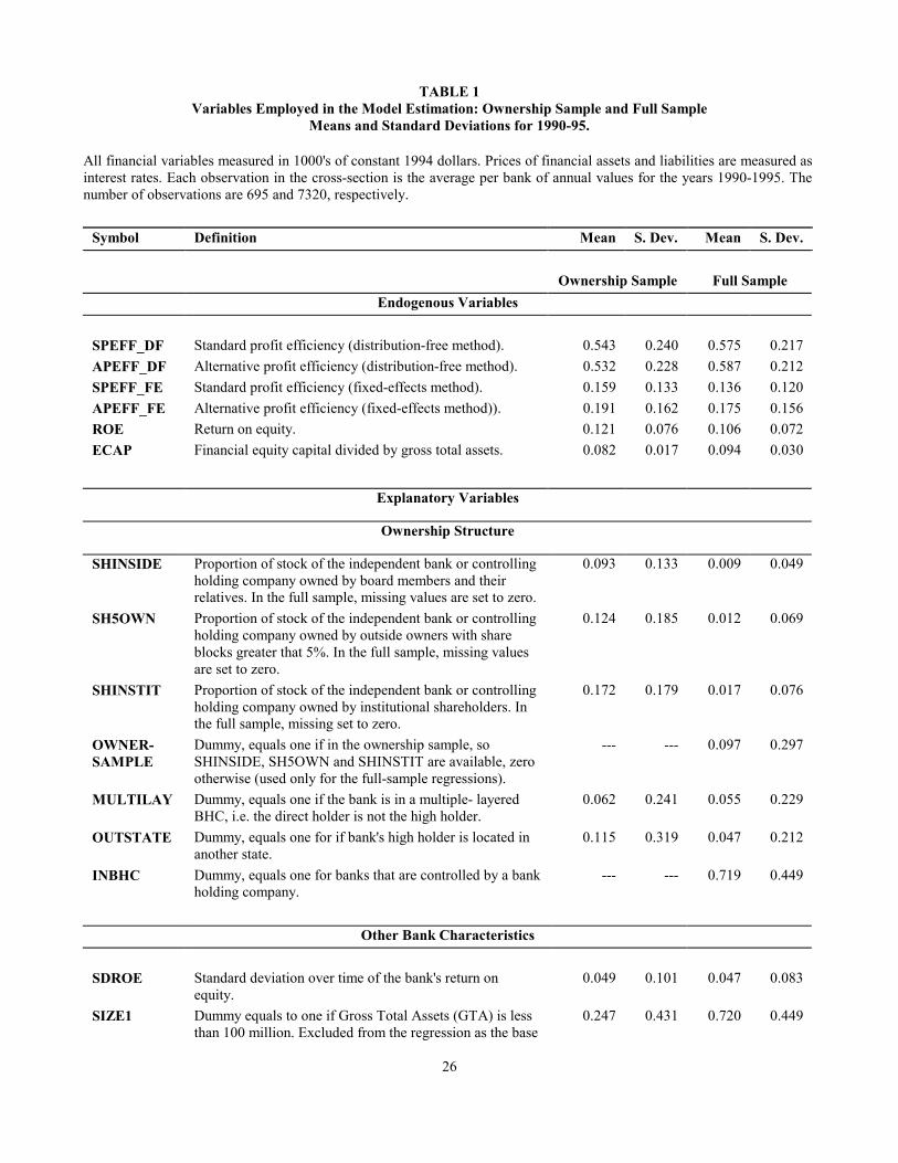
TABLE 1 Variables Employed in the Model Estimation: Ownership Sample and Full Sample

Means and Standard Deviations for 1990-95.

All financial variables measured in 1000's of constant 1994 dollars. Prices of financial assets and liabilities are measured as interest rates. Each observation in the cross-section is the average per bank of annual values for the years 1990-1995. The number of observations are 695 and 7320, respectively.

Symbol Definition Mean S. Dev. Mean S. Dev. Ownership Sample Full Sample

Endogenous Variables SPEFF_DF Standard profit efficiency (distribution-free method). 0.543 0.240 0.575 0.217 APEFF_DF Alternative profit efficiency (distribution-free method). 0.532 0.228 0.587 0.212 SPEFF_FE Standard profit efficiency (fixed-effects method). 0.159 0.133 0.136 0.120 APEFF_FE Alternative profit efficiency (fixed-effects method)). 0.191 0.162 0.175 0.156 ROE Return on equity. 0.121 0.076 0.106 0.072 ECAP Financial equity capital divided by gross total assets. 0.082 0.017 0.094 0.030

Explanatory Variables

Ownership Structure

SHINSIDE Proportion of stock of the independent bank or controlling holding company owned by board members and their relatives. In the full sample, missing values are set to zero.

0.093 0.133 0.009 0.049

SH5OWN Proportion of stock of the independent bank or controlling holding company owned by outside owners with share blocks greater that 5%. In the full sample, missing values are set to zero.

0.124 0.185 0.012 0.069

SHINSTIT Proportion of stock of the independent bank or controlling holding company owned by institutional shareholders. In the full sample, missing set to zero.

0.172 0.179 0.017 0.076

OWNER-SAMPLE

Dummy, equals one if in the ownership sample, so SHINSIDE, SH5OWN and SHINSTIT are available, zero otherwise (used only for the full-sample regressions).

--- --- 0.097 0.297

MULTILAY Dummy, equals one if the bank is in a multiple- layered BHC, i.e. the direct holder is not the high holder.

0.062 0.241 0.055 0.229

OUTSTATE Dummy, equals one for if bank's high holder is located in another state.

0.115 0.319 0.047 0.212

INBHC Dummy, equals one for banks that are controlled by a bank holding company.

--- --- 0.719 0.449

Other Bank Characteristics

SDROE Standard deviation over time of the bank's return on

equity. 0.049 0.101 0.047 0.083

SIZE1 Dummy equals to one if Gross Total Assets (GTA) is less than 100 million. Excluded from the regression as the base

0.247 0.431 0.720 0.449

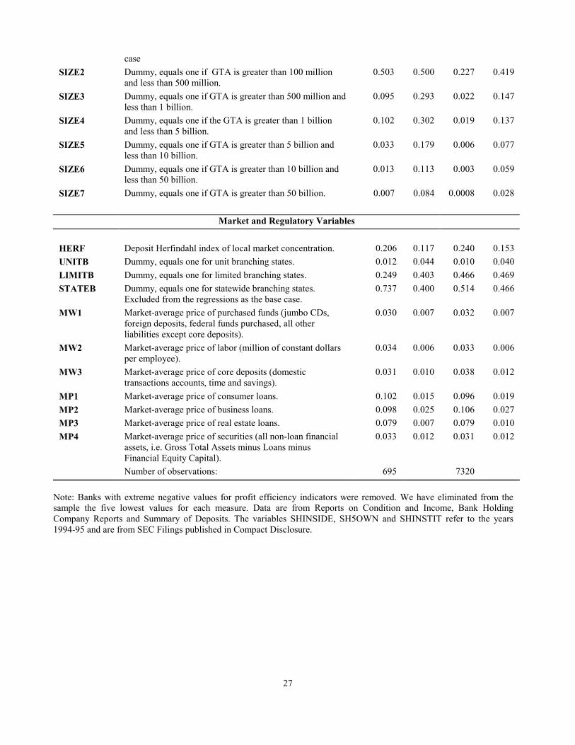
27

case SIZE2 Dummy, equals one if GTA is greater than 100 million

and less than 500 million. 0.503 0.500 0.227 0.419

SIZE3 Dummy, equals one if GTA is greater than 500 million and less than 1 billion.

0.095 0.293 0.022 0.147

SIZE4 Dummy, equals one if the GTA is greater than 1 billion and less than 5 billion.

0.102 0.302 0.019 0.137

SIZE5 Dummy, equals one if GTA is greater than 5 billion and less than 10 billion.

0.033 0.179 0.006 0.077

SIZE6 Dummy, equals one if GTA is greater than 10 billion and less than 50 billion.

0.013 0.113 0.003 0.059

SIZE7 Dummy, equals one if GTA is greater than 50 billion. 0.007 0.084 0.0008 0.028

Market and Regulatory Variables HERF Deposit Herfindahl index of local market concentration. 0.206 0.117 0.240 0.153 UNITB Dummy, equals one for unit branching states. 0.012 0.044 0.010 0.040 LIMITB Dummy, equals one for limited branching states. 0.249 0.403 0.466 0.469 STATEB Dummy, equals one for statewide branching states.

Excluded from the regressions as the base case. 0.737 0.400 0.514 0.466

MW1 Market-average price of purchased funds (jumbo CDs, foreign deposits, federal funds purchased, all other liabilities except core deposits).

0.030 0.007 0.032 0.007

MW2 Market-average price of labor (million of constant dollars per employee).

0.034 0.006 0.033 0.006

MW3 Market-average price of core deposits (domestic transactions accounts, time and savings).

0.031 0.010 0.038 0.012

MP1 Market-average price of consumer loans. 0.102 0.015 0.096 0.019 MP2 Market-average price of business loans. 0.098 0.025 0.106 0.027 MP3 Market-average price of real estate loans. 0.079 0.007 0.079 0.010 MP4 Market-average price of securities (all non-loan financial

assets, i.e. Gross Total Assets minus Loans minus Financial Equity Capital).

0.033 0.012 0.031 0.012

Number of observations: 695 7320

Note: Banks with extreme negative values for profit efficiency indicators were removed. We have eliminated from the sample the five lowest values for each measure. Data are from Reports on Condition and Income, Bank Holding Company Reports and Summary of Deposits. The variables SHINSIDE, SH5OWN and SHINSTIT refer to the years 1994-95 and are from SEC Filings published in Compact Disclosure.

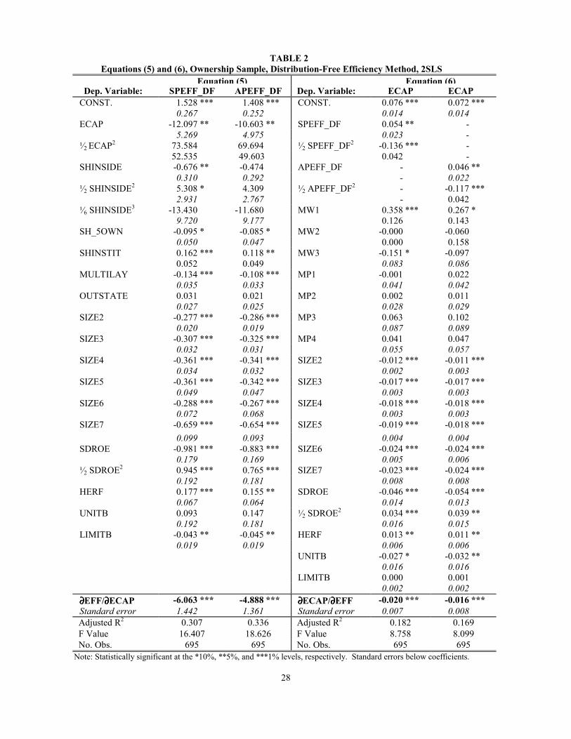
28

TABLE 2 Equations (5) and (6), Ownership Sample, Distribution-Free Efficiency Method, 2SLS

Equation (5) Equation (6)Dep. Variable: SPEFF_DF APEFF_DF Dep. Variable: ECAP ECAP

CONST. 1.528 *** 1.408 *** CONST. 0.076 *** 0.072 *** 0.267 0.252 0.014 0.014 ECAP -12.097 ** -10.603 ** SPEFF_DF 0.054 ** - 5.269 4.975 0.023 - ¹⁄2 ECAP2 73.584 69.694 ¹⁄2 SPEFF_DF2 -0.136 *** - 52.535 49.603 0.042 - SHINSIDE -0.676 ** -0.474 APEFF_DF - 0.046 ** 0.310 0.292 - 0.022 ¹⁄2 SHINSIDE2 5.308 * 4.309 ¹⁄2 APEFF_DF2 - -0.117 *** 2.931 2.767 - 0.042 ¹⁄6 SHINSIDE3 -13.430 -11.680 MW1 0.358 *** 0.267 * 9.720 9.177 0.126 0.143 SH_5OWN -0.095 * -0.085 * MW2 -0.000 -0.060 0.050 0.047 0.000 0.158 SHINSTIT 0.162 *** 0.118 ** MW3 -0.151 * -0.097 0.052 0.049 0.083 0.086 MULTILAY -0.134 *** -0.108 *** MP1 -0.001 0.022 0.035 0.033 0.041 0.042 OUTSTATE 0.031 0.021 MP2 0.002 0.011 0.027 0.025 0.028 0.029 SIZE2 -0.277 *** -0.286 *** MP3 0.063 0.102 0.020 0.019 0.087 0.089 SIZE3 -0.307 *** -0.325 *** MP4 0.041 0.047 0.032 0.031 0.055 0.057 SIZE4 -0.361 *** -0.341 *** SIZE2 -0.012 *** -0.011 *** 0.034 0.032 0.002 0.003 SIZE5 -0.361 *** -0.342 *** SIZE3 -0.017 *** -0.017 *** 0.049 0.047 0.003 0.003 SIZE6 -0.288 *** -0.267 *** SIZE4 -0.018 *** -0.018 *** 0.072 0.068 0.003 0.003 SIZE7 -0.659 *** -0.654 *** SIZE5 -0.019 *** -0.018 *** 0.099 0.093 0.004 0.004 SDROE -0.981 *** -0.883 *** SIZE6 -0.024 *** -0.024 *** 0.179 0.169 0.005 0.006 ¹⁄2 SDROE2 0.945 *** 0.765 *** SIZE7 -0.023 *** -0.024 *** 0.192 0.181 0.008 0.008 HERF 0.177 *** 0.155 ** SDROE -0.046 *** -0.054 *** 0.067 0.064 0.014 0.013 UNITB 0.093 0.147 ¹⁄2 SDROE2 0.034 *** 0.039 ** 0.192 0.181 0.016 0.015 LIMITB -0.043 ** -0.045 ** HERF 0.013 ** 0.011 ** 0.019 0.019 0.006 0.006 UNITB -0.027 * -0.032 ** 0.016 0.016 LIMITB 0.000 0.001 0.002 0.002 ∂∂∂∂EFF/∂∂∂∂ECAP -6.063 *** -4.888 *** ∂∂∂∂ECAP/∂∂∂∂EFF -0.020 *** -0.016 *** Standard error 1.442 1.361 Standard error 0.007 0.008 Adjusted R2 0.307 0.336 Adjusted R2 0.182 0.169 F Value 16.407 18.626 F Value 8.758 8.099 No. Obs. 695 695 No. Obs. 695 695

Note: Statistically significant at the *10%, **5%, and ***1% levels, respectively. Standard errors below coefficients.

29

TABLE 3 Equation (5), Ownership Sample, OLS

Standard Profit and Alternative Profit Efficiency by Distribution-Free Efficiency Method and ROE

OLS OLS OLS OLS Variable SPEFF_DF APEFF_DF ROE ROE CONST. 1.123 *** 0.989 *** 0.203 *** 0.1658 *** 0.118 0.111 0.031 0.051 ECAP -3.926 * -2.253 -0.890 -0.791 2.289 2.158 0.597 0.594 ¹⁄2 ECAP2 -5.620 -9.820 1.523 0.683 22.673 21.372 5.916 5.876 SHINSIDE -0.724 ** -0.521 * -0.106 -0.104 0.305 0.288 0.080 0.079 ¹⁄2 SHINSIDE2 5.541 * 4.528 * 0.328 0.313 2.897 2.731 0.756 0.752 ¹⁄6 SHINSIDE3 -13.801 -11.985 0.311 0.379 9.611 9.059 2.508 2.497 SH5OWN -0.076 -0.066 0.011 0.008 0.048 0.046 0.013 0.013 SHINSTIT 0.177 *** 0.134 *** 0.031 ** 0.036 *** 0.051 0.048 0.013 0.013 MULTILAY -0.137 *** -0.110 *** 0.017 * 0.015 0.035 0.033 0.009 0.009 OUTSTATE 0.031 0.020 -0.012 * -0.012 * 0.026 0.024 0.007 0.007 SIZE2 -0.274 *** -0.282 *** 0.009 * 0.012 ** 0.019 0.018 0.005 0.005 SIZE3 -0.300 *** -0.316 *** 0.006 0.012 0.023 0.028 0.008 0.008 SIZE4 -0.351 *** -0.328 *** 0.011 0.013 0.030 0.028 0.008 0.008 SIZE5 -0.343 *** -0.322 *** 0.038 *** 0.041 *** 0.046 0.043 0.012 0.012 SIZE6 -0.272 *** -0.248 *** 0.019 0.023 0.068 0.064 0.018 0.018 SIZE7 -0.625 *** -0.616 *** 0.009 0.029 0.094 0.088 0.024 0.026 SDROE -0.840 *** -0.732 *** -0.846 *** -0.804 *** 0.150 0.141 0.039 0.041 ¹⁄2 SDROE2 0.840 *** 0.654 *** 0.446 *** 0.405 *** 0.177 0.167 0.046 0.048 HERF 0.173 *** 0.150 ** 0.062 *** 0.045 ** 0.066 0.062 0.017 0.019 UNITB 0.107 0.168 0.132 *** 0.086 * 0.182 0.171 0.047 0.051 LIMITB -0.045 ** -0.048 ** 0.017 *** 0.015 *** 0.020 0.018 0.005 0.006 MP1-4, MW1-3 - - - Not shown - - - ∂∂∂∂ Dep.var./∂∂∂∂ECAP -4.387 *** -3.058 *** -0.765 *** -0.735 *** Standard error 0.609 0.575 0.158 0.158 Adjusted R2 0.355 0.364 0.579 0.588 F value 20.157 20.932 48.758 37.774 No. Obs. 695 695 695 695

*Significant at the 10%, **5%, and *1% levels, respectively. Standard errors below coefficients.

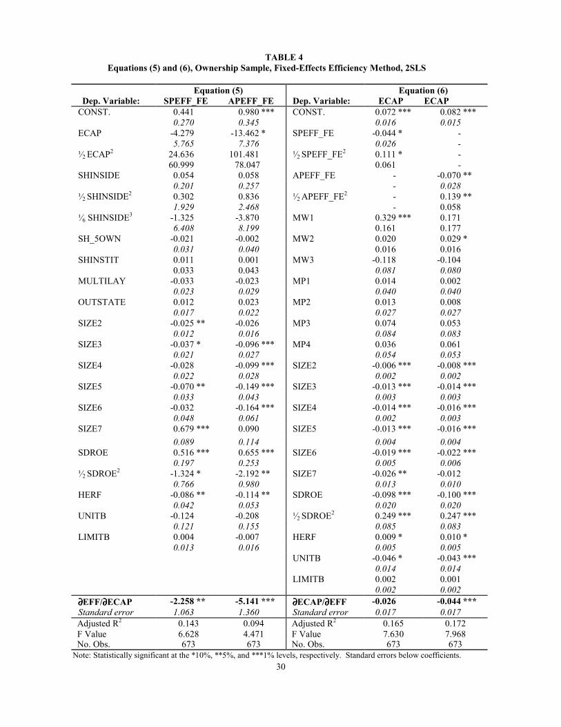
30

TABLE 4 Equations (5) and (6), Ownership Sample, Fixed-Effects Efficiency Method, 2SLS

Equation (5) Equation (6) Dep. Variable: SPEFF_FE APEFF_FE Dep. Variable: ECAP ECAP

CONST. 0.441 0.980 *** CONST. 0.072 *** 0.082 *** 0.270 0.345 0.016 0.015 ECAP -4.279 -13.462 * SPEFF_FE -0.044 * - 5.765 7.376 0.026 - ¹⁄2 ECAP2 24.636 101.481 ¹⁄2 SPEFF_FE2 0.111 * - 60.999 78.047 0.061 - SHINSIDE 0.054 0.058 APEFF_FE - -0.070 ** 0.201 0.257 - 0.028 ¹⁄2 SHINSIDE2 0.302 0.836 ¹⁄2 APEFF_FE2 - 0.139 ** 1.929 2.468 - 0.058 ¹⁄6 SHINSIDE3 -1.325 -3.870 MW1 0.329 *** 0.171 6.408 8.199 0.161 0.177 SH_5OWN -0.021 -0.002 MW2 0.020 0.029 * 0.031 0.040 0.016 0.016 SHINSTIT 0.011 0.001 MW3 -0.118 -0.104 0.033 0.043 0.081 0.080 MULTILAY -0.033 -0.023 MP1 0.014 0.002 0.023 0.029 0.040 0.040 OUTSTATE 0.012 0.023 MP2 0.013 0.008 0.017 0.022 0.027 0.027 SIZE2 -0.025 ** -0.026 MP3 0.074 0.053 0.012 0.016 0.084 0.083 SIZE3 -0.037 * -0.096 *** MP4 0.036 0.061 0.021 0.027 0.054 0.053 SIZE4 -0.028 -0.099 *** SIZE2 -0.006 *** -0.008 *** 0.022 0.028 0.002 0.002 SIZE5 -0.070 ** -0.149 *** SIZE3 -0.013 *** -0.014 *** 0.033 0.043 0.003 0.003 SIZE6 -0.032 -0.164 *** SIZE4 -0.014 *** -0.016 *** 0.048 0.061 0.002 0.003 SIZE7 0.679 *** 0.090 SIZE5 -0.013 *** -0.016 *** 0.089 0.114 0.004 0.004 SDROE 0.516 *** 0.655 *** SIZE6 -0.019 *** -0.022 *** 0.197 0.253 0.005 0.006 ¹⁄2 SDROE2 -1.324 * -2.192 ** SIZE7 -0.026 ** -0.012 0.766 0.980 0.013 0.010 HERF -0.086 ** -0.114 ** SDROE -0.098 *** -0.100 *** 0.042 0.053 0.020 0.020 UNITB -0.124 -0.208 ¹⁄2 SDROE2 0.249 *** 0.247 *** 0.121 0.155 0.085 0.083 LIMITB 0.004 -0.007 HERF 0.009 * 0.010 * 0.013 0.016 0.005 0.005 UNITB -0.046 * -0.043 *** 0.014 0.014 LIMITB 0.002 0.001 0.002 0.002 ∂∂∂∂EFF/∂∂∂∂ECAP -2.258 ** -5.141 *** ∂∂∂∂ECAP/∂∂∂∂EFF -0.026 -0.044 *** Standard error 1.063 1.360 Standard error 0.017 0.017 Adjusted R2 0.143 0.094 Adjusted R2 0.165 0.172 F Value 6.628 4.471 F Value 7.630 7.968No. Obs. 673 673 No. Obs. 673 673

Note: Statistically significant at the *10%, **5%, and ***1% levels, respectively. Standard errors below coefficients.

31

TABLE 5 Equations (5) and (6), Full Sample, Distribution-Free Efficiency Method, 2SLS

Equation (5) Equation (6) Dep. Variable: SPEFF_DF APEFF_DF Dep. Variable: ECAP ECAP CONST. 1.629 *** 1.570 *** CONST. 0.214 *** 0.226 *** 0.072 0.075 0.008 0.009 ECAP -12.797 *** -11.499 *** SPEFF_DF -0.075 *** - 1.146 1.196 0.013 - ¹⁄2 ECAP2 56.275 *** 49.112 *** ¹⁄2 SPEFF_DF2 -0.077 *** - 8.828 9.218 0.023 - SHINSIDE -0.657 ** -0.488 * APEFF - -0.089 *** 0.281 0.293 - 0.011 ¹⁄2 SHINSIDE2 5.439 ** 4.773 * ¹⁄2 APEFF_DF2 - -0.053 *** 2.676 2.794 - 0.019 ¹⁄6 SHINSIDE3 -15.154 * -14.325 MW1 -0.350 *** -0.718 *** 8.892 9.284 0.067 0.082 SH5OWN -0.170 *** -0.164 *** MW2 -0.771 *** -1.136 *** 0.044 0.046 0.080 0.102 SHINSTIT 0.104 ** 0.068 MW3 -0.102 *** 0.052 0.043 0.045 0.038 0.040 OWNERSAMPLE 0.051 *** 0.036 ** MP1 0.003 0.047 ** 0.013 0.014 0.017 0.019 INBHC -0.010 -0.020 ** MP2 -0.035 ** -0.009 0.007 0.007 0.014 0.015 MULTILAY 0.019 * 0.018 * MP3 -0.065 * 0.003 0.010 0.011 0.033 0.036 OUTSTATE 0.003 -0.007 MP4 0.069 ** 0.097 *** 0.012 0.013 0.027 0.030 SIZE2-7 Not Shown Not Shown SIZE2-7 Not Shown Not shown - - - - SDROE -1.955 *** -1.159 *** SDROE -0.149 *** -0.180 *** 0.078 0.081 0.008 0.008 ¹⁄2SDROE2 1.147 *** 1.412 *** ¹⁄2 SDROE2 0.177 *** 0.234 *** 0.139 0.145 0.017 0.013 HERF 0.078 *** 0.076 *** HERF 0.006 *** 0.003 0.015 0.016 0.002 0.002 UNITB 0.102 * 0.203 *** UNITB 0.004 0.002 0.055 0.057 0.008 0.008 LIMITB -0.042 *** -0.046 *** LIMITB -0.002 *** -0.003 *** 0.005 0.005 0.001 0.001 ∂∂∂∂EFF/∂∂∂∂ECAP -7.507 *** -6.881 *** ∂∂∂∂EFF/∂∂∂∂ECAP -0.120 *** -0.119 *** Standard error 0.415 0.432 Standard error 0.005 0.006 Adjusted R2 0.241 0.241 Adjusted R2 0.171 0.143 F value 106.486 106.481 F value 76.715 62.052 No. Obs. 7320 7320 No. Obs. 7320 7320

Note: Significant at the *10%, **5%, and ***1% levels, respectively. Standard errors below coefficients.

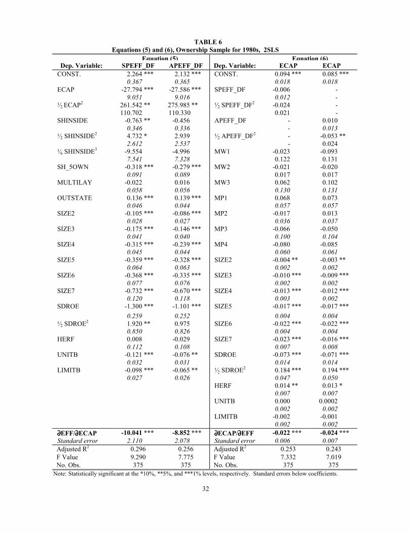
32

TABLE 6 Equations (5) and (6), Ownership Sample for 1980s, 2SLS

Equation (5) Equation (6)Dep. Variable: SPEFF_DF APEFF_DF Dep. Variable: ECAP ECAP

CONST. 2.264 *** 2.132 *** CONST. 0.094 *** 0.085 *** 0.367 0.365 0.018 0.018 ECAP -27.794 *** -27.586 *** SPEFF_DF -0.006 - 9.051 9.016 0.012 - ¹⁄2 ECAP2 261.542 ** 275.985 ** ¹⁄2 SPEFF_DF2 -0.024 - 110.702 110.330 0.021 - SHINSIDE -0.763 ** -0.456 APEFF_DF - 0.010 0.346 0.336 - 0.013 ¹⁄2 SHINSIDE2 4.732 * 2.939 ¹⁄2 APEFF_DF2 - -0.053 ** 2.612 2.537 - 0.024 ¹⁄6 SHINSIDE3 -9.554 -4.996 MW1 -0.023 -0.093 7.541 7.328 0.122 0.131 SH_5OWN -0.318 *** -0.279 *** MW2 -0.021 -0.020 0.091 0.089 0.017 0.017 MULTILAY -0.022 0.016 MW3 0.062 0.102 0.058 0.056 0.130 0.131 OUTSTATE 0.136 *** 0.139 *** MP1 0.068 0.073 0.046 0.044 0.057 0.057 SIZE2 -0.105 *** -0.086 *** MP2 -0.017 0.013 0.028 0.027 0.036 0.037 SIZE3 -0.175 *** -0.146 *** MP3 -0.066 -0.050 0.041 0.040 0.100 0.104 SIZE4 -0.315 *** -0.239 *** MP4 -0.080 -0.085 0.045 0.044 0.060 0.061 SIZE5 -0.359 *** -0.328 *** SIZE2 -0.004 ** -0.003 ** 0.064 0.063 0.002 0.002 SIZE6 -0.368 *** -0.335 *** SIZE3 -0.010 *** -0.009 *** 0.077 0.076 0.002 0.002 SIZE7 -0.732 *** -0.670 *** SIZE4 -0.013 *** -0.012 *** 0.120 0.118 0.003 0.002 SDROE -1.300 *** -1.101 *** SIZE5 -0.017 *** -0.017 *** 0.259 0.252 0.004 0.004 ¹⁄2 SDROE2 1.920 ** 0.975 SIZE6 -0.022 *** -0.022 *** 0.850 0.826 0.004 0.004 HERF 0.008 -0.029 SIZE7 -0.023 *** -0.016 *** 0.112 0.108 0.007 0.008 UNITB -0.121 *** -0.076 ** SDROE -0.073 *** -0.071 *** 0.032 0.031 0.014 0.014 LIMITB -0.098 *** -0.065 ** ¹⁄2 SDROE2 0.184 *** 0.194 *** 0.027 0.026 0.047 0.050 HERF 0.014 ** 0.013 * 0.007 0.007 UNITB 0.000 0.0002 0.002 0.002 LIMITB -0.002 -0.001 0.002 0.002 ∂∂∂∂EFF/∂∂∂∂ECAP -10.041 *** -8.852 *** ∂∂∂∂ECAP/∂∂∂∂EFF -0.022 *** -0.024 *** Standard error 2.110 2.078 Standard error 0.006 0.007 Adjusted R2 0.296 0.256 Adjusted R2 0.253 0.243 F Value 9.290 7.775 F Value 7.332 7.019 No. Obs. 375 375 No. Obs. 375 375

Note: Statistically significant at the *10%, **5%, and ***1% levels, respectively. Standard errors below coefficients.

33

Figure 1

Equation (5): Estimated SPEFF_DF and APEFF_DF as functions of ECAP, Ownership Sample, 2SLS

(Table 2, Columns 1 and 2)

Note: all the other variables are set at the sample mean.

0

0.1

0.2

0.3

0.4

0.5

0.6

0.7

0.8

0.05 0.07 0.08 0.1 0.11 0.13 0.14 0.16 0.17 0.19 0.2 0.22

SPEFF_DF as a function of ECAPAPEFF_DF as a function of ECAP

34

Figure 2

Equation (6): Estimated ECAP as function of SPEFF and APEFF, Ownership Sample, 2SLS (Table 2, Columns 3 and 4)

Note: all the other variables are set at the sample mean.

0.05

0.055

0.06

0.065

0.07

0.075

0.08

0.085

0.09

0.095

0.01 0.11 0.21 0.31 0.41 0.51 0.61 0.71 0.81 0.91 1

ECAP as a function of SPEFF_DFECAP as a function of APEFF_DF

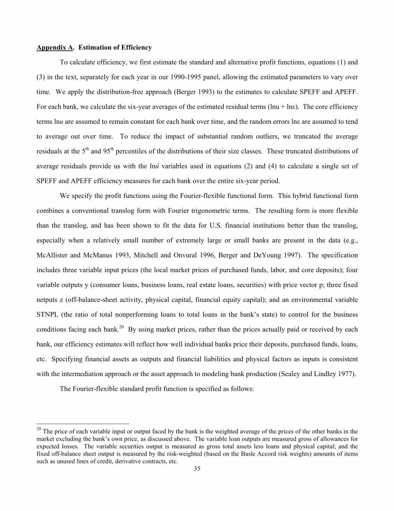
35

Appendix A. Estimation of Efficiency

To calculate efficiency, we first estimate the standard and alternative profit functions, equations (1) and

(3) in the text, separately for each year in our 1990-1995 panel, allowing the estimated parameters to vary over

time. We apply the distribution-free approach (Berger 1993) to the estimates to calculate SPEFF and APEFF.

For each bank, we calculate the six-year averages of the estimated residual terms (lnu + lnε). The core efficiency

terms lnu are assumed to remain constant for each bank over time, and the random errors lnε are assumed to tend

to average out over time. To reduce the impact of substantial random outliers, we truncated the average

residuals at the 5th and 95th percentiles of the distributions of their size classes. These truncated distributions of

average residuals provide us with the lnu variables used in equations (2) and (4) to calculate a single set of

SPEFF and APEFF efficiency measures for each bank over the entire six-year period.

We specify the profit functions using the Fourier-flexible functional form. This hybrid functional form

combines a conventional translog form with Fourier trigonometric terms. The resulting form is more flexible

than the translog, and has been shown to fit the data for U.S. financial institutions better than the translog,

especially when a relatively small number of extremely large or small banks are present in the data (e.g.,

McAllister and McManus 1993, Mitchell and Onvural 1996, Berger and DeYoung 1997). The specification

includes three variable input prices (the local market prices of purchased funds, labor, and core deposits); four

variable outputs y (consumer loans, business loans, real estate loans, securities) with price vector p; three fixed

netputs z (off-balance-sheet activity, physical capital, financial equity capital); and an environmental variable

STNPL (the ratio of total nonperforming loans to total loans in the bank’s state) to control for the business

conditions facing each bank.20 By using market prices, rather than the prices actually paid or received by each

bank, our efficiency estimates will reflect how well individual banks price their deposits, purchased funds, loans,

etc. Specifying financial assets as outputs and financial liabilities and physical factors as inputs is consistent

with the intermediation approach or the asset approach to modeling bank production (Sealey and Lindley 1977).

The Fourier-flexible standard profit function is specified as follows:

20 The price of each variable input or output faced by the bank is the weighted average of the prices of the other banks in the market excluding the bank’s own price, as discussed above. The variable loan outputs are measured gross of allowances for expected losses. The variable securities output is measured as gross total assets less loans and physical capital; and the fixed off-balance sheet output is measured by the risk-weighted (based on the Basle Accord risk weights) amounts of items such as unused lines of credit, derivative contracts, etc.

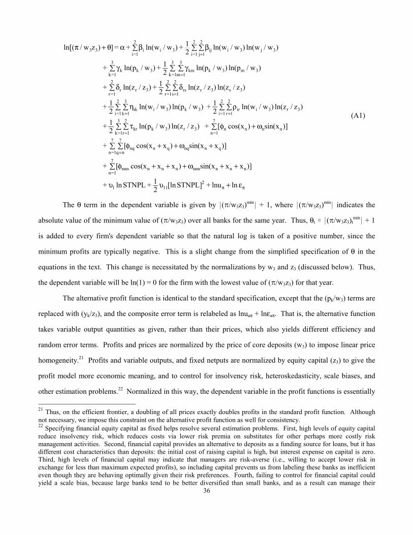
36

ππ

=

=

==

=

=

=

ε+υυ

++ω+++φ�

+ω++φ� �

� ω+φ� � τ

� �ρ� �η

� � �δδ

� � � γγ

� � �ββαθ+π

lnlnu + ]STNPL[ln21 + STNPLln +

)]xxx(sin)xxxcos([ +

)]xx(sin)xxcos([ +

)]x(sin)xcos([ + )z/zln()w/pln(21 +

)z/zln()w/wln(21 + )w/pln()w/wln(2

1 +

)z/zln()z/zln(21 + )z/zln( +

)w/pln()w/pln(21 + )w/pln( +

)w/wln()w/wln(21 + )w/wln( + = ])zw/ln[(

2111

nnnnnnnnnnnn

7

1=n

qnnqqnnq

7

1=n

7

nq

7

1=nnnnn

3

1=k3r

2

1r3kkr

2

1=i3r

2

1r3iir

2

1=i3k

3

1k3iik

2

1=r

2

1=r3s

2

1s3rrs3rr

3

1=k

3

1=k3m

3

1m3kkm3kk

2

1=i

2

1=i3j

2

1j3iij3ii33

(A1)

The θ term in the dependent variable is given by �(�/w3z3)min� + 1, where �(�/w3z3)min� indicates the

absolute value of the minimum value of (�/w3z3) over all banks for the same year. Thus, θt � �(�/w3z3)tmin� + 1

is added to every firm's dependent variable so that the natural log is taken of a positive number, since the

minimum profits are typically negative. This is a slight change from the simplified specification of θ in the

equations in the text. This change is necessitated by the normalizations by w3 and z3 (discussed below). Thus,

the dependent variable will be ln(1) = 0 for the firm with the lowest value of (�/w3z3) for that year.

The alternative profit function is identical to the standard specification, except that the (pk/w3) terms are

replaced with (yk/z3), and the composite error term is relabeled as lnuaπ + lnεaπ. That is, the alternative function

takes variable output quantities as given, rather than their prices, which also yields different efficiency and

random error terms. Profits and prices are normalized by the price of core deposits (w3) to impose linear price

homogeneity.21 Profits and variable outputs, and fixed netputs are normalized by equity capital (z3) to give the

profit model more economic meaning, and to control for insolvency risk, heteroskedasticity, scale biases, and

other estimation problems.22 Normalized in this way, the dependent variable in the profit functions is essentially 21 Thus, on the efficient frontier, a doubling of all prices exactly doubles profits in the standard profit function. Although not necessary, we impose this constraint on the alternative profit function as well for consistency. 22 Specifying financial equity capital as fixed helps resolve several estimation problems. First, high levels of equity capital reduce insolvency risk, which reduces costs via lower risk premia on substitutes for other perhaps more costly risk management activities. Second, financial capital provides an alternative to deposits as a funding source for loans, but it has different cost characteristics than deposits: the initial cost of raising capital is high, but interest expense on capital is zero. Third, high levels of financial capital may indicate that managers are risk-averse (i.e., willing to accept lower risk in exchange for less than maximum expected profits), so including capital prevents us from labeling these banks as inefficient even though they are behaving optimally given their risk preferences. Fourth, failing to control for financial capital could yield a scale bias, because large banks tend to be better diversified than small banks, and as a result can manage their

37

the bank’s return on equity, a measure of how well the bank is using its scarce financial capital. We add 1 to the

arguments (yk/z3), (zr /z3), and STNPL in order to avoid taking the natural log of zero. The xn terms, n=1,...,7 are

re-scaled values of the ln(wi/w3), i=1,2; ln(yk/z3), k=1,2,3 (ln(pk/w3), k=1,2, 3 in the case of the standard profit

function); and ln(zr /z3), r=1,2 terms. To conserve degrees of freedom, we include only the ‘own’ third-order

Fourier terms (e.g., cos(xn + xn + xn)), and exclude the third-order interactions (e.g., cos(xn + xm + xq), m, q ≠

n).23 The standard symmetry restrictions apply to the translog portion of the function (βij = βji, γkm = γmk, δrs =

δsr). We exclude consideration of share equations embodying Hotelling's Lemma restrictions because these

would impose the undesirable assumption of no allocative inefficiencies. We estimate the profit equations using

ordinary least squares.

portfolio risk with lower levels of financial capital. We use an accounting measure of equity because market values are unavailable for most banks. 23 The Fourier-flexible form is a global approximation because the cos xn, sin xn, cos 2xn, sin 2xn, etc., terms are mutually orthogonal over the [0,2π] interval (π refers here to radians, not profits), so that each additional term can make the approximating function closer to the true path of the data wherever it is most needed. The orthogonality is perfect only if the data are evenly distributed over the [0,2π] interval, but in practice the Fourier terms have improved the fit of the data in every application of which we are aware. We cut 10% off each end of the [0,2π] interval so that the xn span [0.1×2π, 0.9×2π] to reduce approximation problems near the endpoints. The formula for xn is 0.2π - µ×a + µ×variable, where [a,b] is the range of the variable being transformed, and µ ≡ (0.9×2π - 0.1×2π)/(b-a).