Research Division Federal Reserve Bank of St. Louis Working Paper Series

Capital Flows and Japanese Asset Volatility

Christopher J. Neely and

Brett W. Fawley

Working Paper 2011-034B

http://research.stlouisfed.org/wp/2011/2011-034.pdf

October 2011 Revised January 2012

FEDERAL RESERVE BANK OF ST. LOUIS Research Division

P.O. Box 442 St. Louis, MO 63166

______________________________________________________________________________________

The views expressed are those of the individual authors and do not necessarily reflect official positions of the Federal Reserve Bank of St. Louis, the Federal Reserve System, or the Board of Governors.

Federal Reserve Bank of St. Louis Working Papers are preliminary materials circulated to stimulate discussion and critical comment. References in publications to Federal Reserve Bank of St. Louis Working Papers (other than an acknowledgment that the writer has had access to unpublished material) should be cleared with the author or authors.

Capital Flows and Japanese Asset Volatility

Christopher J. Neely*

Brett W. Fawley

December 22, 2011

Abstract: Characterizing asset price volatility is an important goal for financial economists. The literature has shown that variables that proxy for the information arrival process can help explain and/or forecast volatility. Unfortunately, however, obtaining good measures of volume and/or order flow is expensive or difficult in decentralized markets such as foreign exchange. We investigate the extent that Japanese capital flows—which are released weekly—reflect information arrival that improves foreign exchange and equity volatility forecasts. We find that capital flows can help explain transitory shocks to GARCH volatility. Keywords: volatility, capital flows, GARCH, exchange rates JEL Codes: F31, F32 * Corresponding author. Send correspondence to Chris Neely, Box 442, Federal Reserve Bank of St. Louis, St. Louis, MO 63166-0442; e-mail: neely@stls.frb.org; phone: 314-444-8568; fax: 314-444-8731. Brett Fawley’s email: brett.w.fawley@stls.frb.org; phone: 314-444-8571. Christopher J. Neely is an assistant vice president and economist at the Federal Reserve Bank of St. Louis. Brett W. Fawley is a Senior Research Associate at the Federal Reserve Bank of St. Louis. The authors are responsible for errors. The views expressed in this paper are those of the authors and do not necessarily reflect those of the Federal Reserve Bank of St. Louis or the Federal Reserve System.

1

I. Introduction

Characterizing asset price volatility is an important goal for financial economists because

of volatility’s role in option pricing and risk management. For example, asset holders dislike

volatile asset prices because they are risk averse; loss of wealth puts their planned consumption

at risk. Similarly, excessive losses put traders’ jobs at risk so they must quantify and restrict the

volatility of their positions. Understanding and estimating asset price volatility is therefore

important for asset pricing, portfolio allocation, and risk management. Therefore, a large

literature has sought to characterize patterns in conditional variance.

Asset prices should equal the present discounted value of expected future fundamentals.

In the case of exchange rates for example, those fundamentals include output and money

supplies. Volatility should be proportional to changes in these expectations of future discounted

fundamentals. News that changes expectations about discount rates or fundamentals should

create changes in asset prices. Because news is persistent — and perhaps because sensitivity to

news is persistent —asset price volatility tends to be persistent.

Engle’s (1982) autoregressive conditionally heteroskedastic (ARCH) model that

characterized the serial correlation in volatility sparked the modern literature on volatility

estimation. Bollerslev (1986) extended the ARCH class to the generalized autoregressive

conditionally heteroskedastic (GARCH) model. Foreign exchange volatility is particularly

important because of the size and depth of foreign exchange markets and the intimate connection

with international trade in goods, services and assets. Baillie and Bollerslev (1989, 1991) have

used GARCH models to characterize U.S. dollar foreign exchange volatility and Neely (1999)

likewise characterized the volatility in the target zones of the European Monetary System.

2

The literature that specifically attempts to forecast—as opposed to characterize in-

sample—asset price volatility is more modest in size. West and Cho (1995) argued that GARCH

models do not actually forecast very well by conventional standards, though they do outperform

homoskedastic models at short horizons. Andersen and Bollerslev (1998) countered this sort of

reasoning by stating that such forecast evaluation techniques were inappropriate. Specifically,

they argue that GARCH models forecast noisy daily measures of volatility about as well as one

would expect. West, Edison and Cho (1993) report that GARCH specifications outperform

alternative volatility forecast methods when assessed from a utility framework in which

underestimating future volatility generates greater disutility than overestimating. Zou, Rose and

Massey (2007) exploit a different kind of asymmetry, namely that bad news effects volatility

more than good news, and find that a threshold ARCH(1,1) in mean model improves volatility

forecasting in the Australian 3-year Treasury bond futures market. More generally, Andersen,

Bollerslev and Diebold (2007) document volatility forecasting gains from removing jumps from

high frequency volatility measures.

In addition to characterizing serial correlation in volatility, the volatility literature has

documented the links between quantity measures—such as volume and order flow—and asset

price volatility. Lamoureux and Lastrapes (1990) investigate the relation between stock trading

volume and heteroskedasticity, finding that volume measures drive out ARCH effects. But such

analysis is more difficult in the decentralized foreign exchange markets, where there are no

comprehensive indicators of daily volume. Foreign exchange traders sometimes use proxies for total

volume, such as volume measures from futures markets, such as the IMM Commitment of Traders,

or screen-based tick counts or proprietary data from market-making banks. But foreign exchange

volume remains difficult to track.

3

More recently, microstructure theory has inspired researchers to consider the effect of order

flow—signed transaction flows—on volatility. News can affect volatility over a prolonged

period through news announcements that release private information that might generate

conflicting trades and price volatility. Because obtaining order flow data is expensive and/or

difficult, researchers have commonly used proxies for order flow: Cai et al. (2001) use yen

positions held by major market participants, Love and Payne (2008) use and Bauwens, Ben

Omrane, and Giot (2005) use quote frequency. Most researchers have used actual order flow data

from electronic brokers such as Reuters D2000-1 (Evans, 2002), Reuters D2000-2 (Dominguez

and Panthaki, 2006, Carlson and Lo, 2006, Love and Payne, 2008, and Rime, Sarno and Sojli,

2010), or Electronic Brokerage Services (Berger, Chaboud, and Hjalmarsson, 2009). Others have

used proprietary datasets from commercial banks (Savaser, 2006, and Frömmel, Mende, and

Menkhoff, 2008).

The amount of information transmitted —and therefore the volatility induced—depends

on the type of order flow. Financial customers are thought to have better information on asset

prices from their own trading and research, whereas commercial firms are considered to be price

takers that trade to import or export goods. Frömmel, Mende, and Menkhoff (2008) find that

only order flow from banks and financial customers (i.e., informed order flow) is linked to higher

foreign exchange volatility.1

Order flows are difficult to work with and expensive to get. An alternative is to use

capital flows, which are the international purchases or sales of assets. Fortunately, the Japanese

Ministry of Finance publishes weekly capital flow data, which is broken down by Japanese and

non-Japanese investors for money markets, bonds and equities.

1 Informed order flow would be order flow that is generated by private information and speculates on a change in asset prices. In contrast, uninformed order flow would be generated by demands for commercial or hedging purposes and would not be predicated on private information that informs expectations of changes in asset prices.

4

Although microstructure theory does not tightly motivate the relation between capital

flows and foreign exchange volatility, capital flows potentially constitute a source of information

about asset price volatility, similar to that played by volume. Asset prices respond very quickly

to news and thus capital flows are surely closely related to volume and probably more loosely

related to order flow.2 And the varying types of capital might contain different quality of

information about future volatility.

Perhaps because higher frequency capital flow data have not been available for very long,

there has been almost no study of the relationship between capital flows and forex volatility.

Aside from the inclusion of capital flows in the announcement study of Evans and Speight

(2010), there has been essentially no study of the relation between capital flows and foreign

exchange volatility. This paper extends the literature on quantity measures and volatility by

examining the relation between financial market volatility and capital flows. Capital flows and

volatility have a strong contemporaneous correlation in JPY data. In addition, capital flows have

similar, often stronger, effects on Nikkei volatility. These relations do not persist after the

addition of BIS turnover data to the empirical model, however. But in the absence of such

turnover data, capital flow data can improve GARCH volatility estimates.

We wish to explicitly recognize and emphasize to the reader that both capital flows and

volatility are endogenous, meaning that we do not ascribe a structural relation to our reduced

form results. We think, however, that a good characterization of the data can be a useful

component of the structural relations.

2 The link between capital flows and foreign exchange order flow depends primarily on the frequency that foreign asset transactions involve currency transactions. For example, rather than borrowing at home to buy Japanese stocks, a foreign investor may choose to borrow yen in Japan.

5

The remainder of the paper proceeds as follows: Section II presents the data. Sections III

and IV present results on the ability of capital flows to explain realized and GARCH volatility in

Japanese assets, respectively. Section V concludes.

II. The Data

The Japanese Ministry of Finance publically publishes data on “International

Transactions in Securities”—capital flows—on the Thursday following the reporting week.3 The

capital flows classify transactions by residence of transactors, type of security (equity securities,

bonds and notes, or money market instruments), and whether they are sales or purchases. In total,

this sums to 12 different types of capital flows (2 classes of investors, 3 types of securities, 2

types of transactions). These data are the preliminary version of the portfolio investment

statistics included in the Balance of Payments reports, and are available beginning in 2005.4

We consider the effect of all 6 types of capital flows, after summing over sales and

purchases to obtain gross capital flows for each class of investor and security type. i.e.,

, , ,

,

where , is the gross transactions by type of investor inv, in security s, during week t, and

the summation index, i, goes over purchases and sales. The sales and purchases of a given type

of security by a given class of investors tend to be very highly correlated. For example, when

Japanese investors buy a lot of foreign bonds, they also sell a lot of foreign bonds. The

correlation is especially true for non-residents transacting in Japanese equity.

3 http://www.mof.go.jp/english/international_policy/reference/itn_transactions_in_securities/index.htm. Transactions are surveyed from “designated major investors,” which are defined by the Ministry of Finance as “banks, financial instruments firms, insurance companies, investment trust management companies and asset management companies, etc. that were designated by the Minister of Finance in accordance with Article 21 of the Ministerial Ordinance Concerning Report on Foreign Exchange transactions, etc.” 4 The “International Transactions in Securities” series replaced the “Securities Investment at Home and Abroad” series, which ran from April 2001 to December 2004. Unfortunately, the series are not comparable due to a change in methodology.

6

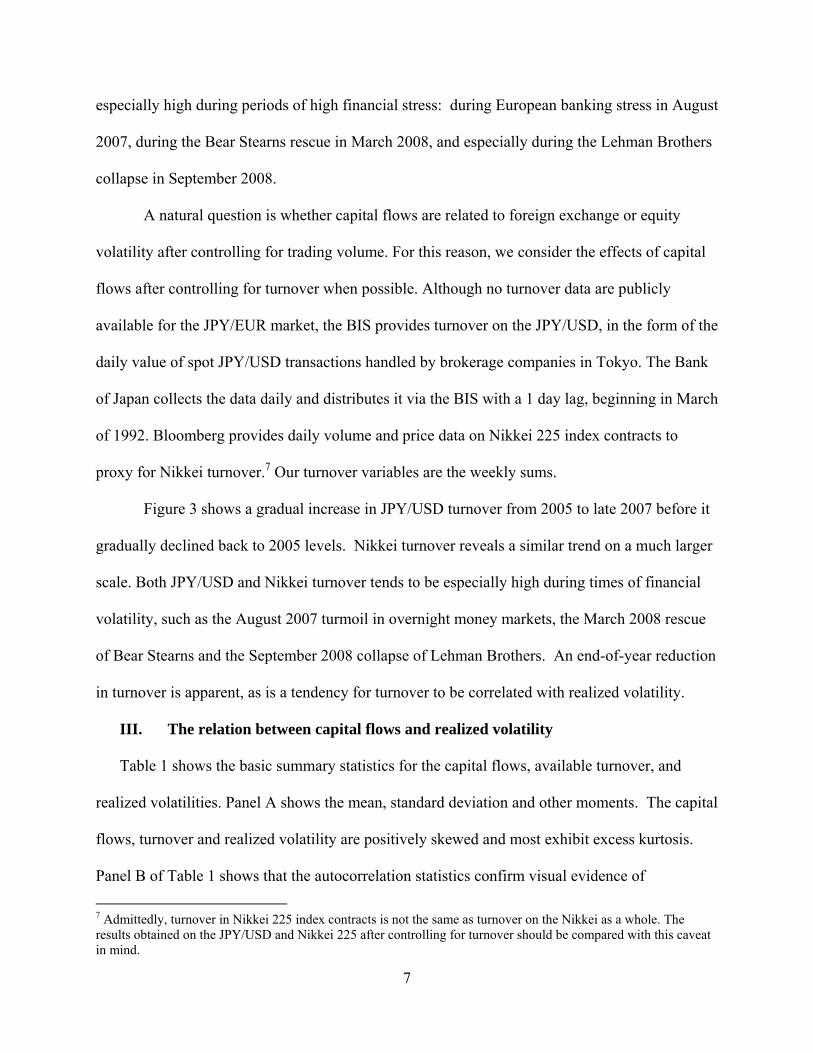
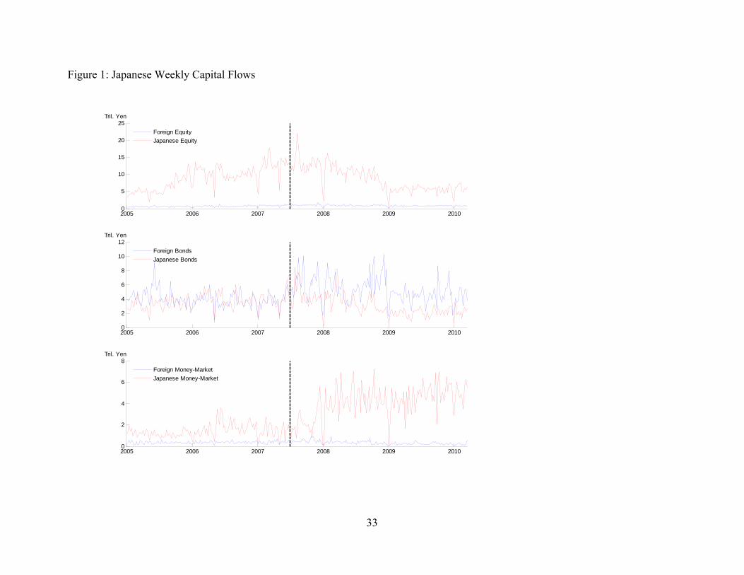
The three panels of Figure 1 show the gross capital flows in equity, bonds and the money

market. The graphs appear to show that the capital flows are basically stationary, with a couple

of exceptions. First, there appears to be a rise in non-Japanese investment in the Japanese money

market in late 2007, just after the start of the financial crisis in the summer of 2007. Second, non-

Japanese investment in Japanese equity surged in late 2005 and remained high until late 2008.

The graphs also appear to show an end-of-year periodic effect, which also appears in the weekly

realized volatility and JPY/USD turnover (see Figures 2 and 3).5

The gross international transactions of non-Japanese investors swamp those of Japanese

investors in both equity and money markets. But the magnitudes of the transactions of the two

types of investors are comparable in bond markets. The Ministry of Finance provides monthly,

disaggregated capital flow data that shows that European investors are the main source of foreign

demand for Japanese bonds, while Japanese investors primarily sell and purchase U.S. bonds.

Disk Trading supplies 5-minute exchange rate data (yen per dollar and yen per euro) from

1/1/2005-3/12/2010. We obtain 5-minute price data for the Nikkei 225 index over the same

sample from TickWrite. For all series, we compute weekly realized volatility as the square root

of the annualized sum of squared returns during each week (Andersen and Bollerslev (1998)).

100 52 ,

where , is the log 5-minute return j during week t.6

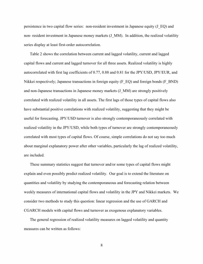
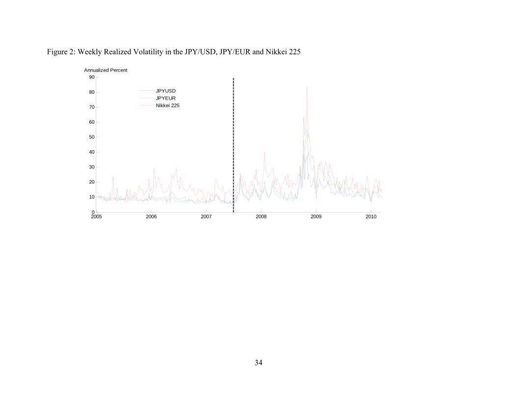
Figure 2 shows the time variation in weekly JPY/USD, EUR/JPY, and Nikkei realized

volatility. Realized volatility increased substantially over the second half of the sample and got

5 Unfortunately, the BIS does not provide data on JPY/EUR turnover or we would use that data as well. 6 We sum over all squared returns from Monday through Friday (measured in EST), excluding returns on Saturday and Sunday.

7

especially high during periods of high financial stress: during European banking stress in August

2007, during the Bear Stearns rescue in March 2008, and especially during the Lehman Brothers

collapse in September 2008.

A natural question is whether capital flows are related to foreign exchange or equity

volatility after controlling for trading volume. For this reason, we consider the effects of capital

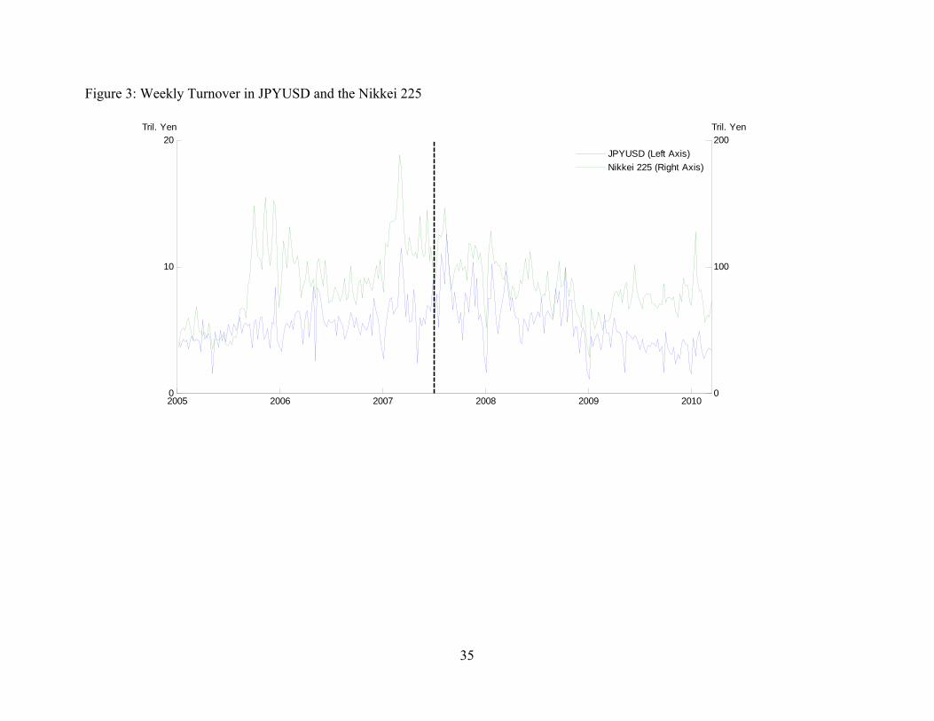
flows after controlling for turnover when possible. Although no turnover data are publicly

available for the JPY/EUR market, the BIS provides turnover on the JPY/USD, in the form of the

daily value of spot JPY/USD transactions handled by brokerage companies in Tokyo. The Bank

of Japan collects the data daily and distributes it via the BIS with a 1 day lag, beginning in March

of 1992. Bloomberg provides daily volume and price data on Nikkei 225 index contracts to

proxy for Nikkei turnover.7 Our turnover variables are the weekly sums.

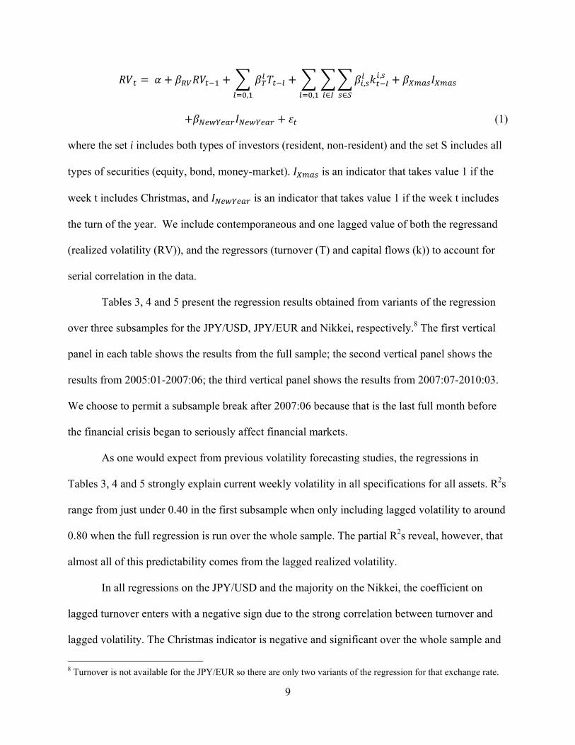
Figure 3 shows a gradual increase in JPY/USD turnover from 2005 to late 2007 before it

gradually declined back to 2005 levels. Nikkei turnover reveals a similar trend on a much larger

scale. Both JPY/USD and Nikkei turnover tends to be especially high during times of financial

volatility, such as the August 2007 turmoil in overnight money markets, the March 2008 rescue

of Bear Stearns and the September 2008 collapse of Lehman Brothers. An end-of-year reduction

in turnover is apparent, as is a tendency for turnover to be correlated with realized volatility.

III. The relation between capital flows and realized volatility

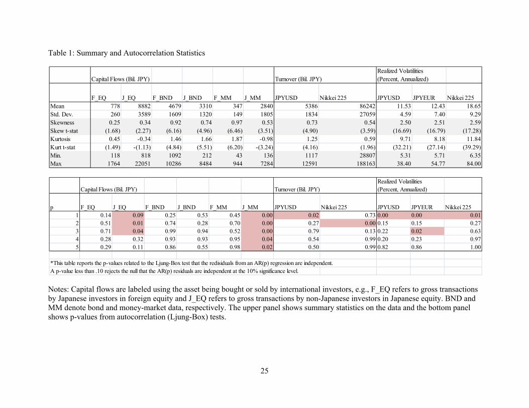
Table 1 shows the basic summary statistics for the capital flows, available turnover, and

realized volatilities. Panel A shows the mean, standard deviation and other moments. The capital

flows, turnover and realized volatility are positively skewed and most exhibit excess kurtosis.

Panel B of Table 1 shows that the autocorrelation statistics confirm visual evidence of

7 Admittedly, turnover in Nikkei 225 index contracts is not the same as turnover on the Nikkei as a whole. The results obtained on the JPY/USD and Nikkei 225 after controlling for turnover should be compared with this caveat in mind.

8

persistence in two capital flow series: non-resident investment in Japanese equity (J_EQ) and

non- resident investment in Japanese money markets (J_MM). In addition, the realized volatility

series display at least first-order autocorrelation.

Table 2 shows the correlation between current and lagged volatility, current and lagged

capital flows and current and lagged turnover for all three assets. Realized volatility is highly

autocorrelated with first lag coefficients of 0.77, 0.88 and 0.81 for the JPY/USD, JPY/EUR, and

Nikkei respectively; Japanese transactions in foreign equity (F_EQ) and foreign bonds (F_BND)

and non-Japanese transactions in Japanese money markets (J_MM) are strongly positively

correlated with realized volatility in all assets. The first lags of those types of capital flows also

have substantial positive correlations with realized volatility, suggesting that they might be

useful for forecasting. JPY/USD turnover is also strongly contemporaneously correlated with

realized volatility in the JPY/USD, while both types of turnover are strongly contemporaneously

correlated with most types of capital flows. Of course, simple correlations do not say too much

about marginal explanatory power after other variables, particularly the lag of realized volatility,

are included.

These summary statistics suggest that turnover and/or some types of capital flows might

explain and even possibly predict realized volatility. Our goal is to extend the literature on

quantities and volatility by studying the contemporaneous and forecasting relation between

weekly measures of international capital flows and volatility in the JPY and Nikkei markets. We

consider two methods to study this question: linear regression and the use of GARCH and

CGARCH models with capital flows and turnover as exogenous explanatory variables.

The general regression of realized volatility measures on lagged volatility and quantity

measures can be written as follows:

9

,

,,

,

(1)

where the set i includes both types of investors (resident, non-resident) and the set S includes all

types of securities (equity, bond, money-market). is an indicator that takes value 1 if the

week t includes Christmas, and is an indicator that takes value 1 if the week t includes

the turn of the year. We include contemporaneous and one lagged value of both the regressand

(realized volatility (RV)), and the regressors (turnover (T) and capital flows (k)) to account for

serial correlation in the data.

Tables 3, 4 and 5 present the regression results obtained from variants of the regression

over three subsamples for the JPY/USD, JPY/EUR and Nikkei, respectively.8 The first vertical

panel in each table shows the results from the full sample; the second vertical panel shows the

results from 2005:01-2007:06; the third vertical panel shows the results from 2007:07-2010:03.

We choose to permit a subsample break after 2007:06 because that is the last full month before

the financial crisis began to seriously affect financial markets.

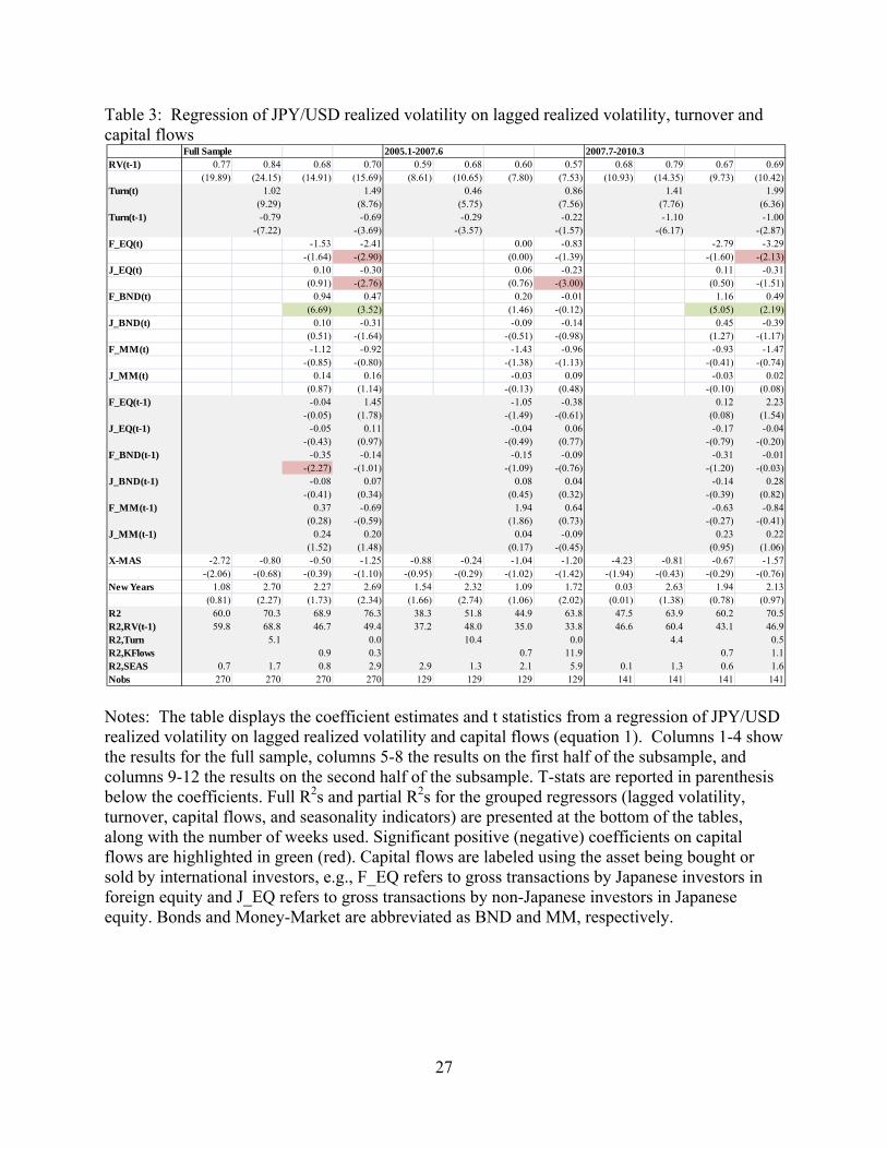
As one would expect from previous volatility forecasting studies, the regressions in

Tables 3, 4 and 5 strongly explain current weekly volatility in all specifications for all assets. R2s

range from just under 0.40 in the first subsample when only including lagged volatility to around

0.80 when the full regression is run over the whole sample. The partial R2s reveal, however, that

almost all of this predictability comes from the lagged realized volatility.

In all regressions on the JPY/USD and the majority on the Nikkei, the coefficient on

lagged turnover enters with a negative sign due to the strong correlation between turnover and

lagged volatility. The Christmas indicator is negative and significant over the whole sample and

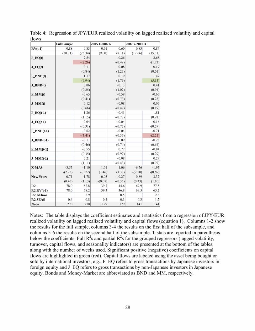
8 Turnover is not available for the JPY/EUR so there are only two variants of the regression for that exchange rate.

10

the second subsample when lagged RV is the only other regressor. It is not significant in most

specifications, however.

Likewise, many of the capital flow variables enter with negative signs due to their

correlation with each other or with turnover. In particular, the lagged values of the capital flow

variables are almost all negative or close to zero. Transactions in equity—both Japanese (J_EQ)

and foreign (F_EQ)—produce negative coefficients for JPY/USD volatility that are significant

across both the full sample and the subsamples when turnover is included. The coefficients on

capital flows into Japanese equity (J_EQ), however, are positive and significant when Nikkei

volatility is the dependent variable. This finding accords with the expectation that increased

foreign activity in the Nikkei would engender higher volatility.

The only significantly positive coefficient for the full sample for all three assets is

contemporaneous Japanese transactions in foreign bonds (F_BND), which is also significant for

the second subsample and marginally significant for the first subsample for each asset. It

becomes less significant when turnover is included in the regression; turnover and foreign bond

transactions have a correlation of 0.48. Examination of the time series in Figure 1 suggests that

Japanese turnover in foreign bonds is unusually high during periods of high financial stress:

August 2007, March 2008 and September 2008. That Japanese bond investors predominantly

transact in U.S. bonds may help explain this correlation, given that these shocks largely

propagated from the US.

Japanese transactions in foreign bonds appear to have significant explanatory power for

weekly JPY/USD volatility. To determine whether the relation is specific to a subsample, we test

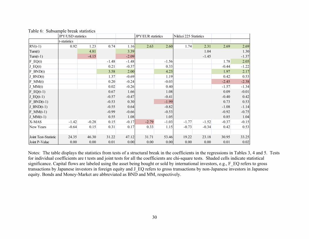
for structural breaks in the coefficients at June/July 2007. Table 6 displays the statistics from

tests of a structural break in the coefficients of Tables 3, 4 and 5. All the joint tests are highly

11

significant, rejecting stability. Among the individual tests (t statistics), the tests for foreign bond

transactions (F_BND) are significant for all assets, and the tests for turnover and foreign equity

(F_EQ) are significant for the JPY/USD and Nikkei, respectively. The coefficients on

contemporaneous foreign bond transactions (F_BND) become (statistically) significantly larger

during the second subsample for all assets. The coefficients on lagged realized volatility are

statistically significantly larger for the JPY/EUR and Nikkei and the point estimates move in the

same direction for the JPY/USD. The coefficients on contemporaneous (lagged) turnover

become larger (smaller) for the JPY/USD.

These results suggest that the explanatory power of contemporaneous foreign bond

transactions (F_BND) for volatility became larger in the second subsample, during the financial

crisis. Overall, the results suggest that although individual capital flows are not usually

significant on their own—except for F_BND—the set of capital flows taken together does

increase the explanatory power of the full volatility regressions even after accounting for lagged

volatility and turnover. The rise in the R2s from the 2nd to the 4th column of the vertical panels in

Tables 3 and 5 support this conclusion. For example, the full sample R2 for the JPY/USD in

Table 3 is 70.3 without the capital flows but rises to 76.3 with the capital flows.

IV. The relation between capital flows and GARCH volatility

There are two interesting reasons, one practical and one theoretical, for asking whether

capital flows can add explanatory power to a GARCH model of asset price volatility. First,

academics and financial practitioners commonly use GARCH to model and forecast asset price

volatility. Could capital flow data improve volatility modeling and forecasting? The second

motivation is to investigate the extent that capital flows may proxy for the underlying

information arrival process driving asset return volatility.

12

Lamoureux and Lastrapes (1990) conjecture that a persistent information arrival process

explains the characteristics of asset price volatility. They describe the volatility process as

following a mixture of distributions model, in which the stochastic rate of information arrival is

the mixing variable. They test this hypothesis by including volume in the conditional variance

equation of the GARCH process for 20 individual US stocks. In line with their prediction, they

find that this proxy for information arrival dramatically reduces the residual persistence captured

by the GARCH parameters.9 Lamoureux and Lastrapes (1990) interpret this result as supporting

the claim that the true driver of persistence in volatility is persistence in information flows, but

that when measures of information arrival are hard to obtain, as they commonly are in foreign

exchange markets, a GARCH model captures the salient features of the volatility process.

Melvin and Yin (2000), on the other hand, use information arrival (headline counts from

Reuters Money Market Headline News) to explain heightened periods of volatility, rather than its

persistence. They include information flow in the conditional mean equation of the GARCH

process instead of the conditional variance equation, permitting news arrival to explain

contemporaneous volatility shocks without directly entering the conditional variance process.

Melvin and Yin (2000) determine that increased public information flows generate increased

volatility and quoting activity, interpreting this as evidence that foreign exchange markets are

efficient processors of new information, and not in need of regulation to minimize alleged self-

churning.

In the spirit of both Lamoureux and Lastrapes (1990) and Melvin and Yin (2000), we use

GARCH models to sequentially investigate the extent that capital flows, and turnover, can

explain transitory and/or persistent volatility in each of our asset price series. The results suggest

9 Their specification was subject to endogeneity issues, and later research showed far weaker conclusions after addressing this endogeneity.

13

that foreign exchange rate volatility often responds contemporaneously to the information shocks

driving capital flows, but that these effects are usually not persistent.

Our analysis considers two baseline specifications of the GARCH process for each asset. The

first specification is the GARCH(1,1) model (Bollerslev, 1986).

1 1

1 1 1

21

t t

t t t

t t t

r c

h z

h h

(2a)

where 1tr is the excess return, 1th is conditional variance and zt has a t distribution.

Our second baseline specification is the component GARCH (CGARCH) model of Engle

and Lee (1999) that characterizes the volatility diffusion process with both a slowly mean

reverting long-run component of conditional variance, qt, and a more volatile, short-run

component, ht – qt.

1 1

1 1 1

21 1

21

t t

t t t

t t t t t t

t t t t

r c

h z

h q q h q

q q h

(2b)

The CGARCH model is helpful in that it permits a slow rate of mean reversion—very persistent

deviations from the mean level of unconditional volatility—that the volatility data in Figure 2

appear to exhibit. To test for the preferred specification, we will exploit the fact that the GARCH

model is nested within the CGARCH model if 0.

Because we are interested in testing for capital flows’ impact on asset volatility, including

the persistence of that impact, we extend the GARCH(1,1) and CGARCH models to include

capital flows/turnover in the conditional variance equations, subject to two sets of parameters,

and .

14

GARCH(1,1) with capital flows

1 1

1 1 1

21 1 1( )

t t

t t t

t t t t t

r c

h z

h h k k

(3a)

CGARCH with capital flows

1 1

1 1 1

21 1 1 1

21 2 1

( )

t t

t t t

t t t t t t t t

t t t t t

r c

h z

h q q h q k k

q q h k

(3b)

Capital flows, tk , are first demeaned and normalized by their standard deviation in order

to provide a clear interpretation of the magnitude of 1 and 2 , as well as to facilitate comparison

between coefficients on different capital flows.10

It would be useful to explain the effect of the parameter on the degree of persistence in

the GARCH and CGARCH models. In the unrestricted GARCH model, the effect on of a one

standard deviation shock to capital flows, , is θ1. In period t+1, this shock will propagate to

through the size of the squared error and through the effect on lagged volatility.

(4)

where is the conditional variance that would have existed in the absence of any capital flow

shock. The expected change to the squared error term is11

(5)

(6)

10 The use of demeaned capital controls could, in principle, produce negative estimates of conditional variance for a sufficiently large positive value of θ1 or θ2. In practice, this was not remotely an issue. 11 Note that we are treating capital flow shocks as strictly exogenous to the GARCH volatility process. In other words, the expectation of is independent of the realization of the capital flow shock.

15

Using (6) in (3a), a one unit shock to capital flows at time t produces the following change in

conditional variance at time t+1

(7)

When is restricted to equal , the capital flow shocks are purely transitory, they do not

persist into the future; when is freely estimated, a small value will make the effect of capital

flow shocks persist. In the CGARCH model, the dynamics are a bit more complex because a

temporary shock to capital can also affect the long-run component, but the general idea is the

same: The amount of persistence depends negatively on the value of .

The parameter identifies the immediate effect of capital flows/turnover on the

conditional variance process because it allows them to directly affect the conditional variance

term, which mean-reverts geometrically. In contrast, 0 and can allow capital

flows to have a more persistent effect on volatility by affecting the slowly mean-reverting

component. In our analysis, we consider the unrestricted model with and as free parameters

and the restriction that 0 and that imposes a purely transitory effect on capital

flows. Capital flows mostly affect conditional volatility contemporaneously if 0.

Alternatively, if 0, the impact of capital flows on the conditional variance process decays at

the same rate as the other conditional variance components, and we are left with the empirical

specification of Lamoureux and Lastrapes (1990).

We estimate the GARCH and CGARCH specifications above with weekly return and

capital flow/turnover data. The weekly returns are computed from the same price series used to

compute realized volatility, but measured at a daily frequency.

The nested nature of the GARCH equations in (2a)-(2b) and (3a)-(3b) allows us to select

models sequentially, testing down from general to specific forms: First, we test whether we can

16

reject the GARCH(1,1) model in favor of the less restrictive CGARCH. Second, we examine

whether including transitory capital flows and or turnover in the volatility equation improves the

model fit ( 0). Finally, we investigate whether the model fit further improves when capital

flows are permitted to influence the persistent volatility process ( 0, ).

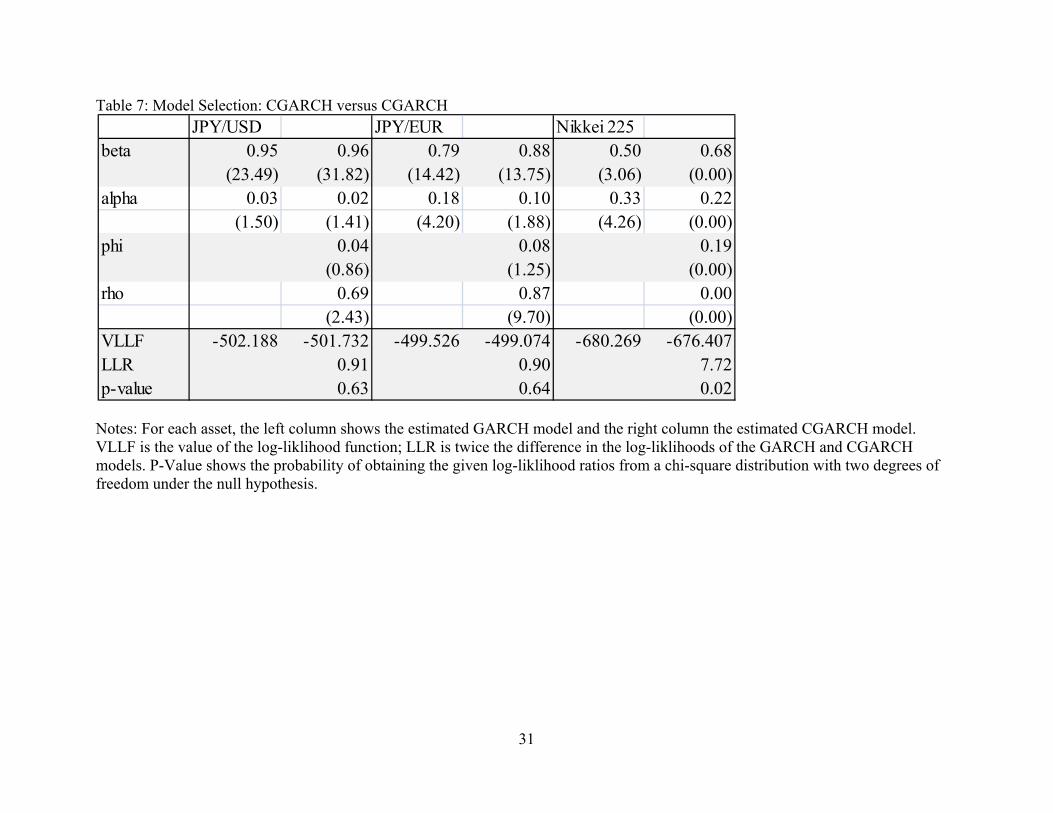
Table 7 shows results from the first stage estimation. The data cannot reject the

restriction to a GARCH process for foreign exchange returns but do reject this restricted model

in favor of the more profligate CGARCH process for the Nikkei returns.

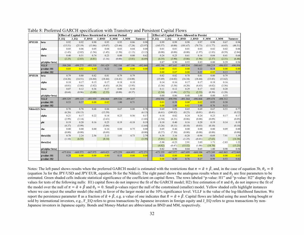
Given these preferred (C)GARCH specifications, we next investigate whether or not

transitory capital flows add explanatory power. The left panel of Table 8 presents the result of

estimating the preferred GARCH model for each asset with capital flows restricted to only

impact current period volatility, i.e., we estimate equations (3a) and (3b) with the restrictions that

and 0.12 Hypothesis 1 (H1) is that transitory capital flows do not improve the

fit of the model without any capital flow effects on volatility (i.e., 0).

Increased capital flows are consistently correlated with heightened volatility in the

current period for all three assets. In particular, log-likelihood ratios indicate that Japanese

transactions in foreign bonds (F_BND) significantly explain GARCH volatility in all three

markets. The point estimates indicate that a one standard deviation increase in Japanese

transactions in foreign bond (F_BND) markets increases the conditional variance of weekly

JPY/USD, JPY/EUR, and Nikkei returns by 0.74, 0.36, and 2.13 percentage points, respectively

(column 1, rows “theta” and “theta1(h)”). The finding that Japanese transactions in foreign bonds

(J_BND) significantly raises transient volatility in all three markets confirms the conclusion of

12 To conserve space, we report results exclusively for the preferred GARCH specification for each asset, i.e. the GARCH(1,1) model for foreign exchange returns and the CGARCH model for equity returns. CGARCH results with foreign exchange returns and GARCH results with equity returns are available upon request. The inference on capital flows does not depend critically on the type of GARCH model used.

17

the previous section that these flows in particular are most robustly associated with volatility.

Additionally, we find that non-Japanese purchases of Japanese equity (J_EQ) help explain

temporarily high volatility in the JPY/USD and the Nikkei. Market turnover also generates a

statistically significant effect in these markets. Japanese transactions in foreign money-markets

(F_MM) is the only capital flow that has no significant effect in any of the three markets.

Foreign activity in Japanese money-markets (J_MM) has the largest impact on contemporaneous

JPY/USD and Nikkei volatility, while, Japanese activity in foreign bonds (F_BND) registers the

largest impact on JPY/EUR volatility. Figure 1 shows that foreign activity in Japanese markets

(J_EQ and J_MM) is much larger than similar Japanese activity in foreign markets (F_EQ and

F_MM). This fact could explain why J_EQ and J_MM better explain volatility than do F_EQ

and F_MM.

In summary, international flows to and from the Japanese money market and to and from

foreign bond markets are associated with transitory changes in exchange rate volatility. Flows to

and from Japanese equity markets are strongly associated with transitory changes in JPY/USD

volatility. Similarly a variety of flows are associated with transitory changes in Nikkei volatility,

including foreign flows to/from all three types of Japanese instruments and Japanese flows

to/from foreign bond markets.

Next, we freely estimate and and ask whether or not the information process proxied

by capital flows explains the persistent component of volatility. Specifically, we ask whether we

should reject our model of primarily transitory effects in favor of a model with more persistent

effects. The right panel of Table 8 shows results from estimating the preferred GARCH

specifications with and freely estimated.13 Null hypothesis 2 (H2) is that the model with

13 Although it is not fixed, we still restrict to lie between 0 and .

18

primarily transitory effects (left panel) explains the data adequately, that persistent capital flow

effects are not significant (right panel).

The data usually fail to reject the null that capital flows have primarily transitory effects,

and the specifications that do generally estimate a high value of , indicating only marginal

persistence. In 13 of the 20 cases the log likelihoods in the right-hand panel do not much exceed

those in the left-hand panel and the row labeled “p-value: H2” are large; hence the data fail to

reject purely transitory effects in those cases. In 4 of the remaining 7 cases that do reject the

smaller model at the 10% significance level (F_EQ, J_EQ, and F_BND for the JPY/USD and

F_EQ for the Nikkei), is estimated to be at least 82% of , indicating only modest

persistence.14

Still, there are several cases (F_EQ, F_BND, F_MM for the JPY/USD and F_EQ and

F_BND for the JPY/EUR) for which the data reject the smaller model without persistence at the

5% significance level. 15 Estimations in two of these cases (F_MM for the JPY/USD and F_EQ

for the JPY/EUR) imply that 0, yielding the reduced model of full persistence estimated by

Lamoureux and Lastrapes (1990). In sharp contrast to Lamoureux and Lastrapes (1990),

however, the magnitude of the residual persistence captured by the GARCH parameters ( )

remains greater than 0.95 in these cases. While these capital flows have persistent effects, they

are not the primary driver of volatility persistence. Curiously, all of these persistent shocks

pertain to Japanese transactions in foreign asset markets affecting exchange rate volatility.

Overall, these results suggest that the level of information flows, as proxied by capital

flows, are associated with exchange rate volatility, consistent with the results of Melvin and Yin

14 We report as a fraction of in Table 8 for ease of interpretation. 15 The finding that Japanese transactions in foreign money-markets (F_MM) have a statistically significant effect on the persistent JPY/USD volatility process is particularly interesting because we were able to uniformly reject the hypothesis of a transitory effect for all three assets. That said, the estimated effect is very small — is only 0.04.

19

(2000). This supports their claim that foreign exchange markets are responding to information to

adjust prices and quantities to achieve efficient allocations. On the other hand, however, capital

flows do not appear to account for the persistent nature of volatility. The row labeled “p-value:

H2” in Panel B of Table1 shows that the data usually fail to reject the null that capital flows have

only transitory effects; even when we reject the null of no persistence, the inclusion of capital

flows does not substantially attenuate the residual persistence measured by .

Our finding that capital flows cannot fully account for volatility persistence closely

echoes the findings of Berger et al. (2009). Berger et al. (2009) investigate the hypothesis that

persistence in both the rate of information arrival and market sensitivity to information generates

persistence in asset price volatility. In decomposing the two effects, they find evidence that

persistence in market sensitivity to information, and not information arrival, explains the

majority of persistence in euro-dollar exchange rate volatility. Berger et al. (2009) further

observe that their measure of information arrival, integrated squared order flow, simply lacks

enough persistence to explain the highly persistent (fractionally integrated) volatility process. In

contrast, their measure of market sensitivity shows a high degree of persistence. Likewise, in our

study, our (C)GARCH models estimate high persistence for volatility—pseudo long-memory for

the CGARCH model—but the capital flow measures appear to be subject to breaks that do not

have counterparts in the volatility data. Our results add further evidence that, while important,

volume alone cannot fully explain volatility persistence.16

V. Conclusion

We investigate whether international capital flows in and out of Japanese markets help

explain patterns in JYP/USD, EUR/USD and Nikkei volatility. Our analysis is explicitly reduced

16 This statement is further supported by the fact that market turnover, in addition to capital flows, is unable to explain volatility persistence in our estimations.

20

form, we are very cautious about structural interpretations without further study. Understanding

whether or not capital flows are correlated with asset price volatility is important, because

presumably the two should be driven by related information processes. The correlations of

different types of capital flows with asset price volatility lend insight into the type of news that is

important for exchange rate determination.

A variety of capital flows contemporaneously affect volatility in all three Japanese asset

markets. Perhaps not surprisingly, the most consistently influential capital flows—foreign flows

to Japanese money markets (J_MM), equity markets (J_EQ) and Japanese flows to foreign bond

markets (F_BND)—also tend to be the largest flows (Figure 1). Japanese flows to foreign bond

markets (F_BND) are the only type of capital flow that produces both transitory and persistent

effects in both foreign exchange markets. Turnover also consistently explained JPY/USD and

Nikkei volatility, but its effects were not persistent. The Nikkei was sensitive to the broadest

variety of capital flows, even after accounting for the greater average Nikkei volatility. Foreign

transactions in Japanese money markets (J_MM) had the greatest effect on the Nikkei.

Using GARCH and CGARCH models, we investigated the persistence of these capital flow

shocks on volatility, finding that such effects on asset volatility are primarily transitory. The data

usually reject specifications that allow capital flow shocks to persist strongly for multiple

periods. Although most capital flows did not have persistent effects on asset volatility, all of

these persistent shocks pertain to Japanese transactions in foreign asset money markets affecting

exchange rate volatility. Why do Japanese transactions produce more persistent effects than

foreign transactions? Japanese investors might have better private information about Japanese

assets and that their trading releases news that raises volatility and prompts further rounds of

21

trading by less informed traders that keeps volatility high, as in the Evans and Lyons (2005)

study of the effects of order flow.

Analysis of structural breaks in linear models suggests that Japanese transactions in foreign

bond markets are particularly well correlated with volatility in the second subsample (2007.7-

2010.3), after the start of the financial crisis. This raises the issue that both capital flows and

volatility are endogenous, of course, leading us to be cautious about structural interpretations.

Disentangling this structural relationship, however, has implications for understanding a variety

of international financial dynamics, including financial contagion. Flavin and Panopoulou

(2010), for example, find that high volatility periods, such as those associated with financial

crises, tend to increase sensitivity to common shocks (‘shift’ contagion) and create direct pass-

through of idiosyncratic shocks (‘pure’ contagion) among Asian equity markets. A structural

understanding of the increased comovement between volatility and capital flows during the

financial crisis may help to illuminate the mechanisms driving heightened contagion effects

during such periods, as well as inform proper policy responses.

The finding that capital flows are linked to periods of heightened GARCH volatility is

consistent with Melvin and Yin’s (2000) claim that news drives foreign exchange market trading

and volatility.

22

References Andersen, T. G. and T. Bollerslev (1998) ‘Answering the Skeptics: Yes, Standard Volatility

Models do Provide Accurate Forecasts’, International Economic Review 39, 885-905.

Andersen, T. G., T. Bollerslev and F. X. Diebold (2007) ‘Roughing it Up: Including Jump

Components in the Measurement, Modeling, and Forecasting of Return Volatility’, The

Review of Economics and Statistics 89, 701-20.

Baillie R. T. and T. Bollerslev (1989) ‘The Message in Daily Exchange Rates: A Conditional

Variance Tale’, Journal of Business and Economic Statistics 7, 297–305.

Baillie R. T. and T. Bollerslev (1991) ‘Intra day and Inter Market Volatility in Foreign Exchange

Rates’, Review of Economic Studies 58, 565–85.

Bauwens, L., W. Ben Omrane and P. Giot (2005) ‘News Announcements, Market Activity and

Volatility in the Euro/Dollar Foreign Exchange Market’, Journal of International Money

and Finance 24, 1108-25.

Berger, D., A. Chaboud and E. Hjalmarsson (2009) ‘What Drives Volatility Persistence in the

Foreign Exchange Market?’, Journal of Financial Economics 94, 192-213.

Bollerslev, T. (1986) ‘Generalized Autoregressive Conditional Heteroskedasticity’, Journal of

Economometrics 31, 307-27.

Cai, J., Y-L. Cheung, R. S. K. Lee and M. Melvin (2001) ‘‘Once-in-a-Generation’ Yen Volatility

in 1998: Fundamentals, Intervention, and Order Flow’, Journal of International Money

and Finance 20, 327-47.

Carlson, J. A. and M. Lo (2006) ‘One Minute in the Life of the DM/US$: Public News in an

Electronic Market’, Journal of International Money and Finance 25, 1090-102.

23

Dominguez, K. M. and F. Panthaki (2006) ‘What Defines ‘News’ in Foreign Exchange

Markets?’, Journal of International Money and Finance 25, 168-98.

Engle, R. F. (1982) ‘Autoregressive Conditional Heteroskedasticity with Estimates of the

Variance of U.K. Inflation’, Econometrica 50, 987–1008.

Engle, R. F. and G. Lee (1999) ‘A Long-Run and Short-Run Component Model of Stock Return

Volatility’, in R. Engle and H. White (eds.), Cointegration, Causality and Forecasting,

Oxford University Press.

Evans, M. D. D. (2002) ‘FX Trading and Exchange Rate Dynamics”, Journal of Finance 57,

2405-47.

Evans, M. D. D. and R. K. Lyons, (2005) ‘Do Currency Markets Absorb News Quickly?’

Journal of International Money and Finance, 24, 197-217.

Evans, K. and A. Speight (2010) ‘International Macroeconomic Announcements and Intraday

Euro Exchange Rate Volatility’, Journal of the Japanese and International Economies

24, 552-68.

Flavin, T. J. and E. Panopoulou (2010) ‘Detecting Shift and Pure Contagion in East Asian Equity

Markets: A Unified Approach’, Pacific Economic Review 15, 401-21.

Frömmel, M., A. Mende and L. Menkhoff (2008) ‘Order Flows, News, and Exchange Rate

Volatility’, Journal of International Money and Finance 27, 994-1012.

Lamoureux, C. G. and W. D. Lastrapes (1990) ‘Heteroskedasticity in Stock Return Data: Volume

versus GARCH Effects’, Journal of Finance 45, 221-9.

Love, R. and R. Payne (2008) ‘Macroeconomic News, Order Flows, and Exchange Rates’, Journal of

Financial and Quantitative Analysis 43, 467-88.

Melvin, M. and X. Yin (2000) ‘Public Information Arrival, Exchange Rate Volatility, and Quote

Frequency’, Economic Journal 110, 644-61.

24

Neely, C. (1999) ‘Target Zones and Conditional Volatility: The Role of Realignments’, Journal

of Empirical Finance 6, 177-92.

Rime, D., L. Sarno and E. Sojli (2010) ‘Exchange Rate Forecasting, Order Flow and

Macroeconomic Information’, Journal of International Economics 80, 72-88.

Savaser, T. (2006) ‘Exchange Rate Response to Macro News: Through the Lens of

Microstructure’, Brandeis University, mimeo, January. www.bwl.uni-

kiel.de/phd/downloads/schneider/ws0607/paper_savaser.pdf.

West, K. D. and D. Cho (1995) ‘The Predictive Ability of Several Models of Exchange Rate

Volatility’, Journal of Econometrics 69, 367-91.

West, K. D., H. J. Edison and D. Cho (1993) ‘A Utility-based Comparison of Some Models of

Exchange Rate Volatility’, Journal of International Economics 35, 23-45.

Zhou, L., L. C. Rose and J. F. Pinfold (2007) ‘Asymmetric Information Impacts: Evidence from the

Australian Treasury-Bond Futures Market’, Pacific Economic Review 12, 665-81.

25

Table 1: Summary and Autocorrelation Statistics

Notes: Capital flows are labeled using the asset being bought or sold by international investors, e.g., F_EQ refers to gross transactions by Japanese investors in foreign equity and J_EQ refers to gross transactions by non-Japanese investors in Japanese equity. BND and MM denote bond and money-market data, respectively. The upper panel shows summary statistics on the data and the bottom panel shows p-values from autocorrelation (Ljung-Box) tests.

Capital Flows (Bil. JPY) Turnover (Bil. JPY)

F_EQ J_EQ F_BND J_BND F_MM J_MM JPYUSD Nikkei 225 JPYUSD JPYEUR Nikkei 225Mean 778 8882 4679 3310 347 2840 5386 86242 11.53 12.43 18.65Std. Dev. 260 3589 1609 1320 149 1805 1834 27059 4.59 7.40 9.29Skewness 0.25 0.34 0.92 0.74 0.97 0.53 0.73 0.54 2.50 2.51 2.59Skew t-stat (1.68) (2.27) (6.16) (4.96) (6.46) (3.51) (4.90) (3.59) (16.69) (16.79) (17.28)Kurtosis 0.45 -0.34 1.46 1.66 1.87 -0.98 1.25 0.59 9.71 8.18 11.84Kurt t-stat (1.49) -(1.13) (4.84) (5.51) (6.20) -(3.24) (4.16) (1.96) (32.21) (27.14) (39.29)Min. 118 818 1092 212 43 136 1117 28807 5.31 5.71 6.35Max 1764 22051 10286 8484 944 7284 12591 188163 38.40 54.77 84.00

Realized Volatilities (Percent, Annualized)

Capital Flows (Bil. JPY)

p F_EQ J_EQ F_BND J_BND F_MM J_MM JPYUSD Nikkei 225 JPYUSD JPYEUR Nikkei 2251 0.14 0.09 0.25 0.53 0.45 0.00 0.02 0.73 0.00 0.00 0.012 0.51 0.01 0.74 0.28 0.70 0.00 0.27 0.00 0.15 0.15 0.273 0.71 0.04 0.99 0.94 0.52 0.00 0.79 0.13 0.22 0.02 0.634 0.28 0.32 0.93 0.93 0.95 0.04 0.54 0.99 0.20 0.23 0.975 0.29 0.11 0.86 0.55 0.98 0.02 0.50 0.99 0.82 0.86 1.00

*This table reports the p-values related to the Ljung-Box test that the redisiduals from an AR(p) regression are independent.A p-value less than .10 rejects the null that the AR(p) residuals are independent at the 10% significance level.

Turnover (Bil. JPY)Realized Volatilities (Percent, Annualized)

26

Table 2: Correlations among the variables

Notes: The table shows correlations between the variables, realized volatility (RV), capital flows (KFlows), turnover and the periodic indicators for the week of Christmas and the week of the turn of the year. USD, EUR and Nikkei refer to variables measured on the JPY/USD, JPY/EUR, and Nikkei 225, respectively. Capital flows are labeled using the asset being bought or sold by international investors, e.g., F_EQ refers to gross transactions by Japanese investors in foreign equity and J_EQ refers to gross transactions by non-Japanese investors in Japanese equity. Bonds and Money-Market are abbreviated as BND and MM, respectively.

RV(t) RV(t-1) KFlows(t) KFlows(t-1) Dummies Turnover(t) Turnover(t-1)EUR Nikkei USD EUR Nikkei F_EQ J_EQ F_BND J_BND F_MM J_MM F_EQ J_EQ F_BND J_BND F_MM J_MM X-MAS New Years USD Nikkei USD Nikkei

RV(t) USD 93.6 83.3 77.0 77.0 68.2 23.6 -4.3 47.6 -5.8 -12.3 49.5 17.3 -6.0 36.8 -10.6 -12.0 45.8 -7.5 -2.5 20.6 -13.5 8.8 -14.4EUR 84.2 80.0 88.1 74.2 22.4 -13.4 44.8 -18.5 -18.3 49.2 20.5 -12.8 37.3 -20.4 -18.8 47.4 -4.1 -2.2 7.6 -17.5 1.3 -16.0Nikkei 75.0 76.0 81.1 35.1 18.1 45.6 3.4 -3.4 46.7 26.4 13.8 36.7 -5.9 -6.3 43.0 -8.4 -12.1 29.3 3.5 19.3 4.6

RV(t-1) USD 93.5 83.0 22.1 -12.3 30.9 -13.8 -16.8 48.6 23.1 -4.7 47.4 -6.0 -12.2 49.7 0.8 -7.5 0.0 -18.3 20.3 -13.8EUR 84.1 21.0 -20.3 32.0 -25.1 -22.4 47.3 22.4 -13.2 44.9 -18.5 -18.3 49.4 2.7 -4.1 -7.6 -22.4 7.7 -17.3Nikkei 23.5 3.6 29.0 -9.1 -12.0 42.9 35.5 18.5 45.7 3.5 -3.0 47.3 0.3 -8.3 7.6 -5.8 29.4 4.2

KFlows(t) F_EQ 56.3 49.8 36.0 30.1 28.3 44.8 40.1 30.2 15.6 14.1 18.1 -25.3 -29.1 53.4 37.7 30.7 33.5J_EQ 28.6 68.2 46.6 -7.6 41.8 80.6 12.1 48.6 38.6 -20.1 -17.3 -21.9 81.6 78.7 61.3 70.8F_BND 29.5 23.8 32.4 25.6 14.3 49.9 7.1 10.3 17.7 -22.9 -21.1 48.0 0.2 20.5 -3.6J_BND 38.3 -16.5 21.5 55.1 16.4 61.7 31.8 -27.4 -15.5 -23.6 70.0 44.6 48.2 40.4F_MM -18.3 15.3 38.4 12.0 29.6 36.8 -21.1 -14.7 -20.0 44.1 25.7 32.8 21.9J_MM 25.1 -10.7 31.2 -26.0 -22.9 75.9 -7.8 -15.7 -6.7 -11.5 -11.3 -11.8

KFlows(t-1) F_EQ 56.9 49.9 36.1 30.3 28.8 -1.2 -25.1 29.2 33.0 53.7 38.6J_EQ 28.6 68.1 47.2 -6.7 -1.8 -17.2 64.5 65.2 81.6 78.9F_BND 29.5 24.2 33.0 -1.8 -22.9 21.5 -5.7 48.0 0.5J_BND 38.7 -16.2 0.8 -15.5 46.2 33.8 70.0 44.6F_MM -18.9 -1.9 -14.7 37.7 21.2 44.9 26.3J_MM 4.5 -7.7 -18.8 -20.0 -5.9 -10.6

Dummies X-MAS -1.9 -19.3 -9.1 -7.2 1.9New Years -25.0 -11.7 -19.3 -9.0

Turnover(t) USD 53.5 60.0 50.4Nikkei 42.9 84.6

Turnover(t-1) USD 53.5

27

Table 3: Regression of JPY/USD realized volatility on lagged realized volatility, turnover and capital flows

Notes: The table displays the coefficient estimates and t statistics from a regression of JPY/USD realized volatility on lagged realized volatility and capital flows (equation 1). Columns 1-4 show the results for the full sample, columns 5-8 the results on the first half of the subsample, and columns 9-12 the results on the second half of the subsample. T-stats are reported in parenthesis below the coefficients. Full R2s and partial R2s for the grouped regressors (lagged volatility, turnover, capital flows, and seasonality indicators) are presented at the bottom of the tables, along with the number of weeks used. Significant positive (negative) coefficients on capital flows are highlighted in green (red). Capital flows are labeled using the asset being bought or sold by international investors, e.g., F_EQ refers to gross transactions by Japanese investors in foreign equity and J_EQ refers to gross transactions by non-Japanese investors in Japanese equity. Bonds and Money-Market are abbreviated as BND and MM, respectively.

Full Sample 2005.1-2007.6 2007.7-2010.3RV(t-1) 0.77 0.84 0.68 0.70 0.59 0.68 0.60 0.57 0.68 0.79 0.67 0.69

(19.89) (24.15) (14.91) (15.69) (8.61) (10.65) (7.80) (7.53) (10.93) (14.35) (9.73) (10.42)Turn(t) 1.02 1.49 0.46 0.86 1.41 1.99

(9.29) (8.76) (5.75) (7.56) (7.76) (6.36)Turn(t-1) -0.79 -0.69 -0.29 -0.22 -1.10 -1.00

-(7.22) -(3.69) -(3.57) -(1.57) -(6.17) -(2.87)F_EQ(t) -1.53 -2.41 0.00 -0.83 -2.79 -3.29

-(1.64) -(2.90) (0.00) -(1.39) -(1.60) -(2.13)J_EQ(t) 0.10 -0.30 0.06 -0.23 0.11 -0.31

(0.91) -(2.76) (0.76) -(3.00) (0.50) -(1.51)F_BND(t) 0.94 0.47 0.20 -0.01 1.16 0.49

(6.69) (3.52) (1.46) -(0.12) (5.05) (2.19)J_BND(t) 0.10 -0.31 -0.09 -0.14 0.45 -0.39

(0.51) -(1.64) -(0.51) -(0.98) (1.27) -(1.17)F_MM(t) -1.12 -0.92 -1.43 -0.96 -0.93 -1.47

-(0.85) -(0.80) -(1.38) -(1.13) -(0.41) -(0.74)J_MM(t) 0.14 0.16 -0.03 0.09 -0.03 0.02

(0.87) (1.14) -(0.13) (0.48) -(0.10) (0.08)F_EQ(t-1) -0.04 1.45 -1.05 -0.38 0.12 2.23

-(0.05) (1.78) -(1.49) -(0.61) (0.08) (1.54)J_EQ(t-1) -0.05 0.11 -0.04 0.06 -0.17 -0.04

-(0.43) (0.97) -(0.49) (0.77) -(0.79) -(0.20)F_BND(t-1) -0.35 -0.14 -0.15 -0.09 -0.31 -0.01

-(2.27) -(1.01) -(1.09) -(0.76) -(1.20) -(0.03)J_BND(t-1) -0.08 0.07 0.08 0.04 -0.14 0.28

-(0.41) (0.34) (0.45) (0.32) -(0.39) (0.82)F_MM(t-1) 0.37 -0.69 1.94 0.64 -0.63 -0.84

(0.28) -(0.59) (1.86) (0.73) -(0.27) -(0.41)J_MM(t-1) 0.24 0.20 0.04 -0.09 0.23 0.22

(1.52) (1.48) (0.17) -(0.45) (0.95) (1.06)X-MAS -2.72 -0.80 -0.50 -1.25 -0.88 -0.24 -1.04 -1.20 -4.23 -0.81 -0.67 -1.57

-(2.06) -(0.68) -(0.39) -(1.10) -(0.95) -(0.29) -(1.02) -(1.42) -(1.94) -(0.43) -(0.29) -(0.76)New Years 1.08 2.70 2.27 2.69 1.54 2.32 1.09 1.72 0.03 2.63 1.94 2.13

(0.81) (2.27) (1.73) (2.34) (1.66) (2.74) (1.06) (2.02) (0.01) (1.38) (0.78) (0.97)R2 60.0 70.3 68.9 76.3 38.3 51.8 44.9 63.8 47.5 63.9 60.2 70.5R2,RV(t-1) 59.8 68.8 46.7 49.4 37.2 48.0 35.0 33.8 46.6 60.4 43.1 46.9R2,Turn 5.1 0.0 10.4 0.0 4.4 0.5R2,KFlows 0.9 0.3 0.7 11.9 0.7 1.1R2,SEAS 0.7 1.7 0.8 2.9 2.9 1.3 2.1 5.9 0.1 1.3 0.6 1.6Nobs 270 270 270 270 129 129 129 129 141 141 141 141

28

Table 4: Regression of JPY/EUR realized volatility on lagged realized volatility and capital flows

Notes: The table displays the coefficient estimates and t statistics from a regression of JPY/EUR realized volatility on lagged realized volatility and capital flows (equation 1). Columns 1-2 show the results for the full sample, columns 3-4 the results on the first half of the subsample, and columns 5-6 the results on the second half of the subsample. T-stats are reported in parenthesis below the coefficients. Full R2s and partial R2s for the grouped regressors (lagged volatility, turnover, capital flows, and seasonality indicators) are presented at the bottom of the tables, along with the number of weeks used. Significant positive (negative) coefficients on capital flows are highlighted in green (red). Capital flows are labeled using the asset being bought or sold by international investors, e.g., F_EQ refers to gross transactions by Japanese investors in foreign equity and J_EQ refers to gross transactions by non-Japanese investors in Japanese equity. Bonds and Money-Market are abbreviated as BND and MM, respectively.

Full Sample 2005.1-2007.6 2007.7-2010.3RV(t-1) 0.88 0.83 0.61 0.60 0.83 0.84

(30.71) (23.34) (9.00) (8.11) (17.66) (15.31)F_EQ(t) -2.54 -0.26 -3.68

-(2.26) -(0.49) -(1.73)J_EQ(t) 0.11 0.08 0.17

(0.84) (1.23) (0.61)F_BND(t) 1.17 0.19 1.47

(6.94) (1.79) (5.15)J_BND(t) 0.06 -0.13 0.41

(0.25) -(1.02) (0.94)F_MM(t) -0.65 -0.58 -0.65

-(0.41) -(0.73) -(0.23)J_MM(t) 0.12 -0.08 0.06

(0.66) -(0.47) (0.19)F_EQ(t-1) 1.26 -0.41 1.81

(1.15) -(0.77) (0.91)J_EQ(t-1) -0.04 -0.04 -0.16

-(0.31) -(0.72) -(0.59)F_BND(t-1) -0.62 -0.04 -0.71

-(3.41) -(0.36) -(2.21)J_BND(t-1) -0.11 0.09 -0.28

-(0.46) (0.74) -(0.64)F_MM(t-1) -0.55 0.77 -0.84

-(0.35) (0.97) -(0.29)J_MM(t-1) 0.21 -0.08 0.29

(1.11) -(0.43) (0.97)X-MAS -3.55 -1.10 1.01 1.06 -6.76 -1.95

-(2.25) -(0.72) (1.46) (1.38) -(2.50) -(0.69)New Years 0.71 1.78 -0.03 -0.27 0.89 3.37

(0.45) (1.13) -(0.05) -(0.35) (0.33) (1.10)R2 78.0 82.8 39.7 44.6 69.9 77.5R2,RV(t-1) 78.0 68.2 39.3 36.8 69.5 65.2R2,KFlows 2.9 0.5 2.6R2,SEAS 0.4 0.8 0.4 0.1 0.3 1.7Nobs 270 270 129 129 141 141

29

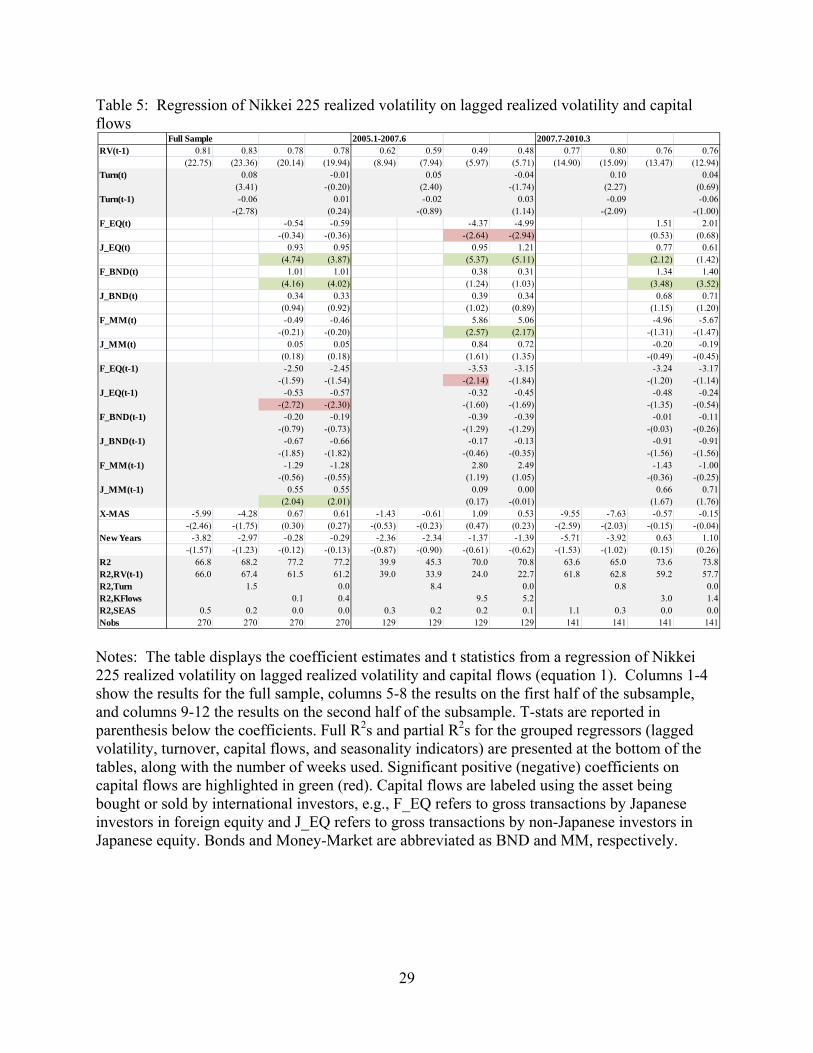
Table 5: Regression of Nikkei 225 realized volatility on lagged realized volatility and capital flows

Notes: The table displays the coefficient estimates and t statistics from a regression of Nikkei 225 realized volatility on lagged realized volatility and capital flows (equation 1). Columns 1-4 show the results for the full sample, columns 5-8 the results on the first half of the subsample, and columns 9-12 the results on the second half of the subsample. T-stats are reported in parenthesis below the coefficients. Full R2s and partial R2s for the grouped regressors (lagged volatility, turnover, capital flows, and seasonality indicators) are presented at the bottom of the tables, along with the number of weeks used. Significant positive (negative) coefficients on capital flows are highlighted in green (red). Capital flows are labeled using the asset being bought or sold by international investors, e.g., F_EQ refers to gross transactions by Japanese investors in foreign equity and J_EQ refers to gross transactions by non-Japanese investors in Japanese equity. Bonds and Money-Market are abbreviated as BND and MM, respectively.

Full Sample 2005.1-2007.6 2007.7-2010.3RV(t-1) 0.81 0.83 0.78 0.78 0.62 0.59 0.49 0.48 0.77 0.80 0.76 0.76

(22.75) (23.36) (20.14) (19.94) (8.94) (7.94) (5.97) (5.71) (14.90) (15.09) (13.47) (12.94)Turn(t) 0.08 -0.01 0.05 -0.04 0.10 0.04

(3.41) -(0.20) (2.40) -(1.74) (2.27) (0.69)Turn(t-1) -0.06 0.01 -0.02 0.03 -0.09 -0.06

-(2.78) (0.24) -(0.89) (1.14) -(2.09) -(1.00)F_EQ(t) -0.54 -0.59 -4.37 -4.99 1.51 2.01

-(0.34) -(0.36) -(2.64) -(2.94) (0.53) (0.68)J_EQ(t) 0.93 0.95 0.95 1.21 0.77 0.61

(4.74) (3.87) (5.37) (5.11) (2.12) (1.42)F_BND(t) 1.01 1.01 0.38 0.31 1.34 1.40

(4.16) (4.02) (1.24) (1.03) (3.48) (3.52)J_BND(t) 0.34 0.33 0.39 0.34 0.68 0.71

(0.94) (0.92) (1.02) (0.89) (1.15) (1.20)F_MM(t) -0.49 -0.46 5.86 5.06 -4.96 -5.67

-(0.21) -(0.20) (2.57) (2.17) -(1.31) -(1.47)J_MM(t) 0.05 0.05 0.84 0.72 -0.20 -0.19

(0.18) (0.18) (1.61) (1.35) -(0.49) -(0.45)F_EQ(t-1) -2.50 -2.45 -3.53 -3.15 -3.24 -3.17

-(1.59) -(1.54) -(2.14) -(1.84) -(1.20) -(1.14)J_EQ(t-1) -0.53 -0.57 -0.32 -0.45 -0.48 -0.24

-(2.72) -(2.30) -(1.60) -(1.69) -(1.35) -(0.54)F_BND(t-1) -0.20 -0.19 -0.39 -0.39 -0.01 -0.11

-(0.79) -(0.73) -(1.29) -(1.29) -(0.03) -(0.26)J_BND(t-1) -0.67 -0.66 -0.17 -0.13 -0.91 -0.91

-(1.85) -(1.82) -(0.46) -(0.35) -(1.56) -(1.56)F_MM(t-1) -1.29 -1.28 2.80 2.49 -1.43 -1.00

-(0.56) -(0.55) (1.19) (1.05) -(0.36) -(0.25)J_MM(t-1) 0.55 0.55 0.09 0.00 0.66 0.71

(2.04) (2.01) (0.17) -(0.01) (1.67) (1.76)X-MAS -5.99 -4.28 0.67 0.61 -1.43 -0.61 1.09 0.53 -9.55 -7.63 -0.57 -0.15

-(2.46) -(1.75) (0.30) (0.27) -(0.53) -(0.23) (0.47) (0.23) -(2.59) -(2.03) -(0.15) -(0.04)New Years -3.82 -2.97 -0.28 -0.29 -2.36 -2.34 -1.37 -1.39 -5.71 -3.92 0.63 1.10

-(1.57) -(1.23) -(0.12) -(0.13) -(0.87) -(0.90) -(0.61) -(0.62) -(1.53) -(1.02) (0.15) (0.26)R2 66.8 68.2 77.2 77.2 39.9 45.3 70.0 70.8 63.6 65.0 73.6 73.8R2,RV(t-1) 66.0 67.4 61.5 61.2 39.0 33.9 24.0 22.7 61.8 62.8 59.2 57.7R2,Turn 1.5 0.0 8.4 0.0 0.8 0.0R2,KFlows 0.1 0.4 9.5 5.2 3.0 1.4R2,SEAS 0.5 0.2 0.0 0.0 0.3 0.2 0.2 0.1 1.1 0.3 0.0 0.0Nobs 270 270 270 270 129 129 129 129 141 141 141 141

30

Table 6: Subsample break statistics

Notes: The table displays the statistics from tests of a structural break in the coefficients in the regressions in Tables 3, 4 and 5. Tests for individual coefficients are t tests and joint tests for all the coefficients are chi-square tests. Shaded cells indicate statistical significance. Capital flows are labeled using the asset being bought or sold by international investors, e.g., F_EQ refers to gross transactions by Japanese investors in foreign equity and J_EQ refers to gross transactions by non-Japanese investors in Japanese equity. Bonds and Money-Market are abbreviated as BND and MM, respectively.

JPY/USD statistics JPY/EUR statistics Nikkei 225 Statisticst-statistics

RV(t-1) 0.92 1.23 0.74 1.16 2.63 2.60 1.74 2.31 2.69 2.69Turn(t) 4.81 3.39 1.04 1.30Turn(t-1) -4.15 -2.09 -1.45 -1.37F_EQ(t) -1.48 -1.48 -1.56 1.78 2.05J_EQ(t) 0.21 -0.37 0.33 -0.44 -1.22F_BND(t) 3.58 2.00 4.23 1.97 2.17J_BND(t) 1.37 -0.69 1.19 0.42 0.53F_MM(t) 0.20 -0.24 -0.03 -2.45 -2.38J_MM(t) 0.02 -0.26 0.40 -1.57 -1.34F_EQ(t-1) 0.67 1.66 1.08 0.09 -0.01J_EQ(t-1) -0.57 -0.47 -0.41 -0.40 0.42F_BND(t-1) -0.53 0.30 -1.99 0.73 0.53J_BND(t-1) -0.55 0.64 -0.82 -1.08 -1.14F_MM(t-1) -0.99 -0.66 -0.53 -0.92 -0.75J_MM(t-1) 0.55 1.08 1.05 0.85 1.04X-MAS -1.42 -0.28 0.15 -0.17 -2.79 -1.03 -1.77 -1.52 -0.37 -0.15New Years -0.64 0.15 0.31 0.17 0.33 1.15 -0.73 -0.34 0.42 0.53

Joint Test-Statistic 24.35 46.30 31.22 47.12 31.71 53.46 19.22 23.18 30.95 33.25Joint P-Value 0.00 0.00 0.01 0.00 0.00 0.00 0.00 0.00 0.01 0.02

31

Table 7: Model Selection: CGARCH versus CGARCH

Notes: For each asset, the left column shows the estimated GARCH model and the right column the estimated CGARCH model. VLLF is the value of the log-liklihood function; LLR is twice the difference in the log-liklihoods of the GARCH and CGARCH models. P-Value shows the probability of obtaining the given log-liklihood ratios from a chi-square distribution with two degrees of freedom under the null hypothesis.

JPY/USD JPY/EUR Nikkei 225beta 0.95 0.96 0.79 0.88 0.50 0.68

(23.49) (31.82) (14.42) (13.75) (3.06) (0.00)alpha 0.03 0.02 0.18 0.10 0.33 0.22

(1.50) (1.41) (4.20) (1.88) (4.26) (0.00)phi 0.04 0.08 0.19

(0.86) (1.25) (0.00)rho 0.69 0.87 0.00

(2.43) (9.70) (0.00)VLLF -502.188 -501.732 -499.526 -499.074 -680.269 -676.407LLR 0.91 0.90 7.72p-value 0.63 0.64 0.02

32

Table 8: Preferred GARCH specification with Transitory and Persistent Capital Flows

Notes: The left panel shows results when the preferred GARCH model is estimated with the restrictions that , and, in the case of equation 3b, 0 (equation 3a for the JPY/USD and JPY/EUR, equation 3b for the Nikkei). The right panel shows the analogous results when and are free parameters to be estimated. Green shaded cells indicate statistical significance of the coefficient on capital flows. The rows labeled “p-value: H1” and “p-value: H2” display the p-values for tests of the following nulls: H1) capital flows do not improve the fit of the GARCH model; H2) free estimation of and do not improve the fit of the model over the null of and 0. Small p-values reject the null of the constrained (smaller) model. Yellow shaded cells highlight instances where we can reject the smaller model (the null) in favor of the larger model at the 10% significance level. VLLF is the value of the log-likelihood function. We report the persistence parameter as a fraction of , e.g. a value of one indicates that . Capital flows are labeled using the asset being bought or sold by international investors, e.g., F_EQ refers to gross transactions by Japanese investors in foreign equity and J_EQ refers to gross transactions by non-Japanese investors in Japanese equity. Bonds and Money-Market are abbreviated as BND and MM, respectively.

Effect of Capital Flows Restricted to Current Period Effect of Capital Flows Allowed to PersistF_EQ J_EQ F_BND J_BND F_MM J_MM Turnover F_EQ J_EQ F_BND J_BND F_MM J_MM Turnover

JPYUSD beta 0.92 0.92 0.90 0.93 0.95 0.86 0.90 0.99 0.99 0.98 0.97 0.98 0.67 0.94(15.51) (25.19) (13.86) (19.07) (23.44) (7.24) (23.97) (165.57) (0.00) (101.67) (70.73) (111.77) (4.43) (48.51)

alpha 0.05 0.06 0.05 0.04 0.03 0.04 0.08 0.01 0.01 0.01 0.03 0.02 0.02 0.06(1.43) (2.02) (1.56) (1.45) (1.50) (1.13) (3.12) (0.00) (0.00) (0.00) (1.97) (1.83) (0.59) (2.84)

theta 0.40 0.51 0.74 0.23 0.00 0.80 0.62 0.24 0.25 0.61 0.16 0.04 0.41 0.68(2.25) (2.83) (4.81) (1.16) (0.00) (3.81) (6.69) (4.35) (3.90) (5.86) (1.96) (2.37) (2.31) (6.48)

pi/(alpha+beta) 0.87 0.90 0.93 0.83 0.00 0.29 0.94VLLF -500.208 -499.275 -493.310 -501.429 -502.188 -497.196 -492.068 -495.196 -497.643 -489.334 -500.663 -500.219 -496.035 -490.894p-value: H1 0.05 0.02 0.00 0.22 1.00 0.00 0.00 0.00 0.01 0.00 0.22 0.14 0.00 0.00p-value: H2 0.00 0.07 0.00 0.22 0.05 0.13 0.13

JPYEUR beta 0.79 0.80 0.82 0.81 0.79 0.79 0.82 0.82 0.78 0.81 0.80 0.79(14.26) (14.51) (16.84) (18.44) (14.41) (14.08) (15.69) (14.02) (16.34) (18.44) (13.83) (13.62)

alpha 0.18 0.17 0.15 0.17 0.18 0.18 0.14 0.16 0.17 0.17 0.18 0.16(4.01) (3.86) (3.82) (4.43) (4.20) (3.95) (3.36) (3.54) (4.20) (4.43) (4.02) (3.56)

theta 0.07 0.12 0.36 0.17 0.00 0.10 0.11 0.12 0.29 0.17 0.02 0.20(0.64) (0.96) (3.40) (2.33) (0.00) (0.37) (2.34) (1.08) (3.71) (2.33) (0.30) (1.28)

pi/(alpha+beta) 0.00 0.86 0.48 1.00 0.00 0.55VLLF -499.329 -499.125 -493.959 -496.868 -499.526 -499.457 -494.956 -498.996 -491.364 -496.868 -499.478 -498.312p-value: H1 0.53 0.37 0.00 0.02 1.00 0.71 0.01 0.59 0.00 0.02 0.95 0.30p-value: H2 0.00 1.00 0.02 1.00 0.76 0.13

Nikkei225 beta 0.70 0.78 0.68 0.84 0.67 0.00 0.78 0.69 0.98 0.65 0.69 0.67 0.53 0.77(6.26) (10.13) (13.39) (6.13) (6.61) (249.82) (0.23) (0.01) (0.41) (0.32)

alpha 0.21 0.17 0.22 0.14 0.23 0.56 0.17 0.18 0.02 0.24 0.24 0.23 0.17 0.17(2.99) (3.14) (2.63) (1.68) (2.54) (4.21) (0.06) (0.00) (0.09) (0.05)

phi 0.19 0.20 0.16 0.25 0.19 -0.18 0.19 0.18 0.40 0.16 0.20 0.19 0.14 0.19(4.37) (5.99) (3.04) (1.64) (3.26) (8.11) (0.10) (0.03) (0.10) (0.10)

rho 0.00 0.00 0.00 0.16 0.00 0.75 0.00 0.05 0.46 0.00 0.00 0.00 0.09 0.00(0.00) (0.00) (0.69) (0.00) (0.37) (7.30) (0.00) (0.00) (0.00) (0.00)

theta1(h) 0.78 2.24 2.56 2.13 1.01 4.73 2.79 6.38 3.16 -0.28 -0.94 -0.69 7.91 1.39(1.10) (6.55) (8.14) (3.39) (5.01) (6.36) -(1.25) -(0.41) -(7.63) (14.38)

theta2(w) -5.98 -0.23 2.91 3.03 1.71 -2.83 1.22-(4.82) -(0.47) (15.52) (1.00) (18.70) (15.25)

pi/(alpha+beta) 0.82 0.96 0.04 0.65 1.00 0.98 0.94VLLF -675.816 -669.573 -667.975 -669.423 -675.259 -664.493 -672.271 -673.339 -667.977 -667.699 -668.106 -675.249 -663.865 -672.069p-value: H1 0.28 0.00 0.00 0.00 0.13 0.00 0.00 0.11 0.00 0.00 0.00 0.51 0.00 0.03p-value: H2 0.08 0.20 0.76 0.27 0.99 0.53 0.82

33

Figure 1: Japanese Weekly Capital Flows

2005 2006 2007 2008 2009 20100

5

10

15

20

25Tril. Yen

Foreign EquityJapanese Equity

2005 2006 2007 2008 2009 20100

2

4

6

8

10

12Tril. Yen

Foreign BondsJapanese Bonds

2005 2006 2007 2008 2009 20100

2

4

6

8Tril. Yen

Foreign Money-MarketJapanese Money-Market

34

Figure 2: Weekly Realized Volatility in the JPY/USD, JPY/EUR and Nikkei 225

2005 2006 2007 2008 2009 20100

10

20

30

40

50

60

70

80

90Annualized Percent

JPYUSDJPYEURNikkei 225

35

Figure 3: Weekly Turnover in JPYUSD and the Nikkei 225

2005 2006 2007 2008 2009 20100

10

20Tril. Yen Tril. Yen

0

100

200JPYUSD (Left Axis)Nikkei 225 (Right Axis)