Capital Accumulation and Structural Transformation∗

Paula Bustos Gabriel Garber Jacopo Ponticelli†

May 31, 2019

Abstract

Several scholars argue that high agricultural productivity growth can retard indus-trial development as it draws resources towards the comparative advantage sector,agriculture. However, agricultural productivity growth can lead to industrializationthrough its impact on capital accumulation. We highlight this effect in a simplemodel where larger agricultural profits increase the supply of capital, generating anexpansion of the capital-intensive sector, manufacturing. To test the predictions ofthe model we exploit a large and exogenous increase in agricultural profits due tothe adoption of genetically engineered soy in Brazil. We find that profits generatedin soy-producing regions were not reinvested locally. Instead, agricultural produc-tivity growth generated capital outflows from rural areas. To trace the destinationof capital flows we match data on deposit and lending activity of all bank branchesin Brazil, bank-firm credit relationships and firm employment. We find that capitalreallocated from soy-producing to non-soy producing regions, and from agricultureto non-agricultural activities. The degree of financial integration affects the speed ofstructural transformation. First, regions that are more financially integrated withsoy-producing areas experienced faster growth in non-agricultural lending. Second,firms that are better connected to soy-producing areas through their pre-existingbanking relationships experienced larger growth in borrowing and employment.

Keywords: Agricultural Productivity, Bank Networks, Financial Integration.JEL Classification: O14, O16, O41, F11

∗We received valuable comments from Abhijit Banerjee, Mark Rosenzweig, Joseph Kaboski, NicolaGennaioli, Douglas Gollin, David Lagakos, Gregor Matvos, Marti Mestieri, Manuel Arellano, Josep PijoanMas, Farzad Saidi, Sergio Mikio Koyama, and seminar participants at NBER Summer Institute - Develop-ment Economics, CEPR-BREAD, CEPR-ESSFM, CEPR-ESSIM, CEPR-ERWIT, Stanford SCID/IGC,BGSE Summer Forum, Dartmouth, Princeton, Berkeley, Chicago Booth, Northwestern Kellogg, UCSD,Columbia Business School, IMF, LSE, Bank of Spain, CREI, Stockholm University, CEMFI, Queen MaryUniversity, FGV-SP, FGV-RJ, and PUC-Rio de Janeiro. We are grateful to acknowledge financial supportfrom the Fama-Miller Center at the University of Chicago, from the PEDL Project by the CEPR, and theEuropean Research Council Starting Grant 716338. Juan Manuel Castro Vincenzi provided outstandingresearch assistance.†Bustos: CEMFI and CEPR, paula.bustos@cemfi.es. Garber: DEPEP, Central Bank

of Brazil, gabriel.garber@bcb.gov.br. Ponticelli: Northwestern University and CEPR, ja-copo.ponticelli@kellogg.northwestern.edu.

1

I Introduction

The process of economic development is characterized by a reallocation of production

factors from the agricultural to the industrial and service sectors. Economic historians

have argued that in the first industrialized countries technical improvements in agricul-

ture favored this process by increasing demand for manufactures or generating savings to

finance industrial projects.1 However, the recent experience of some low-income countries

appears inconsistent with the idea that high agricultural productivity leads to economic

development. The theoretical literature has proposed two sets of explanations. First, the

positive effects of agricultural productivity on economic development might not take place

in open economies where manufactures can be imported and savings can be exported.2

Second, market frictions might constrain factor reallocation.3 The recent empirical lit-

erature has focused on understanding how these mechanisms shape the process of labor

reallocation.4 However, there is scarce direct empirical evidence on the process of capital

reallocation from the rural agricultural sector to the urban industrial sector.5

In this paper we study the effects of productivity growth in agriculture on the allocation

of capital across sectors. To guide the empirical analysis we refer to the Heckscher-Ohlin

model which illustrates the classic effect of agricultural technical change on structural

transformation in an open economy: larger agricultural productivity increases the de-

mand for capital in agriculture, thus capital reallocates towards this sector (Findlay and

Grubert 1959). This is the negative effect of agricultural comparative advantage on in-

dustrialization highlighted in the development literature and we refer to it as the capital

demand effect. In this paper, we present a simple two-period version of the model where

larger agricultural income generates savings, the supply of capital increases and thus the

capital-intensive sector, manufacturing, expands. This positive effect of agricultural pro-

ductivity on industrialization has been overlooked by the literature and will be the main

focus of our empirical analysis. We refer to it as the capital supply effect.

Our empirical analysis attempts to trace the causal effects of agricultural productivity

growth on the allocation of capital across sectors and regions. This has proven challenging

1See, for example, Crafts (1985) and Crouzet (1972). See also Rosenstein-Rodan (1943), Nurkse(1953), Rostow (1960).

2Corden and Neary (1982), Matsuyama (1992).3Banerjee and Newman (1993), Murphy, Shleifer, and Vishny (1989), Galor and Zeira (1993), Ace-

moglu and Zilibotti (1997). See also the recent macroeconomic literature on financial frictions anddevelopment: Gine and Townsend (2004), Jeong and Townsend (2008), Buera, Kaboski, and Shin (2015),Moll (2014).

4For labor reallocation across sectors see McCaig and Pavcnik (2013), Foster and Rosenzweig (2004,2007), Bustos, Caprettini, and Ponticelli (2016); see also Herrendorf, Rogerson, and Valentinyi (2014) fora review of the macro literature. For labor reallocation across regions see: Bryan and Morten (2015),Moretti (2011), Munshi and Rosenzweig (2016). For labor reallocation across sectors and regions see:Michaels, Rauch, and Redding (2012), Fajgelbaum and Redding (2014).

5A notable exception is Banerjee and Munshi (2004) who document larger access to capital for en-trepreneurs belonging to rich agricultural communities in the garment industry in Tirupur, India.

2

for the literature due to the limited availability of data on capital flows within countries.

We overcome this difficulty by using detailed information on deposits and loans for each

bank branch in Brazil. We match this data with confidential information on bank-firm

credit relationships and social security records containing the employment histories for

the universe of formal firms. Therefore, our final dataset permits to observe capital

flows across both sectoral and spatial dimensions. We use this data to establish the

causal effect of agricultural productivity growth on the direction of capital flows. For this

purpose, we exploit a large and exogenous increase in agricultural productivity: namely

the legalization of genetically engineered (GE) soy in Brazil. This new technology had

heterogeneous effects on yields across areas with different soil and weather characteristics,

which permits to estimate the local effects of agricultural productivity growth. However,

because soy producing regions tend to be rural, capital reallocation towards the urban

industrial sector needs to take place across regions. Thus, a second step in our empirical

strategy relies on differences in the degree of financial integration across regions to trace

capital flows from rural to urban areas.

First, we study the local effects of agricultural productivity growth. We find that

municipalities subject to faster exogenous technical change indeed experienced faster

adoption of GE soy and growth in agricultural profits. We think of these municipali-

ties directly affected by agricultural technical change as origin municipalities. Consistent

with the model, we find that these municipalities experienced a larger increase in saving

deposits in local bank branches. However, there was no increase in local bank lending.

As a result, agricultural technical change generated capital outflows from origin munici-

palities. This finding suggests that the increase in the local demand for capital is smaller

than the increase in savings. Thus, banks must have reallocated savings towards other

regions. Therefore, we propose a methodology to track the destination of those savings

generated by agricultural productivity growth.

In a second step of the analysis, we need to trace the reallocation of capital across

space. For this purpose, we exploit differences in the geographical structure of bank

branch networks for 115 Brazilian Banks. We think of these banks as intermediaries

that reallocate savings from origin municipalities to destination municipalities. First, we

show that banks more exposed to the soy boom through their branch network indeed

had a larger increase in aggregate deposits. Next, we track the destination of those

deposits generated by agricultural technical change. For this purpose, we assume that,

due to imperfections in the interbank market, banks are likely to fund part of their loans

with their own deposits. This implies that we can construct exogenous credit supply

shocks across destination municipalities using differences in the geographical structure of

bank branch networks. We use this variation to assess whether destination municipalities

more connected to origin municipalities experiencing agricultural productivity growth

received larger capital inflows. We find that municipalities with relatively larger presence

3

of banks receiving funds from the soy boom experienced faster increases in credit supply.

Interestingly, these funds went entirely to non-soy producing regions and were channeled

to non-agricultural activities.

The findings discussed above are consistent with the capital supply mechanism em-

phasized by the model: agricultural technical change can increase savings and lead to a

reallocation of capital towards the capital intensive sector, manufacturing. Our empirical

analysis permits to quantify this effect by comparing the speed of capital reallocation

across sectors in non-soy producing municipalities with different degrees of financial inte-

gration with the soy boom area. During the period under study (1996-2010), the share

of non-agricultural lending increased from 75 to 84 percent in the average non-soy pro-

ducing municipality. However, the degree of capital reallocation away from agriculture

varied extensively across municipalities: the interquartile range was 22 percentage points.

Our estimates imply that the differences in the degree of financial integration with the

soy boom area can explain 11 percent of the observed differences in the increase in non-

agricultural lending share across non-soy producing municipalities.

As mentioned above, our findings are consistent with the capital supply mechanism

emphasized by the model. However, to the extent that destination municipalities which

are more connected to origin municipalities through bank-branch networks are also more

connected through the transportation or commercial networks, it is possible that our

estimates are capturing the effects of agricultural technical change through other channels.

For example, if technical change is labor-saving, former agricultural workers might migrate

towards cities increasing labor supply, the marginal product of capital and capital demand.

Similarly, cities could face larger product demand from richer farmers. As a result, our

empirical strategy permits to assess the effect of agricultural productivity on the allocation

of capital across sectors but can not isolate whether this occurs through a labor supply,

product demand or capital supply channel. To make progress on this front we need to

implement a firm-level empirical strategy which permits to control for labor supply and

product demand shocks in destination municipalities, which we describe below.

In a third step of the analysis, we trace the reallocation of capital towards firms located

in destination municipalities. For this purpose, we match administrative data on the

credit and employment relationships for the universe of formal firms. We use this data to

construct firm-level exogenous credit supply shocks using information on pre-existing firm-

bank relationships. We use these shocks to assess whether firms whose pre-existing lenders

are more connected to soy-producing regions through bank branch networks experienced

larger increases in borrowing and employment growth. This empirical strategy permits

to isolate the capital supply channel by comparing firms borrowing from different banks

but operating in the same municipality and sector, thus subject to the same labor supply

and product demand shocks.

We find that firms with pre-existing relationships more exposed banks experienced

4

a larger increase in borrowing from those banks. Interestingly, we find similar point

estimates when we control for municipality and sector-level shocks. This suggests that

the increase in firm borrowing is driven by the capital supply effect of agricultural technical

change and not the labor supply or product demand effects. We can use our estimates to

calculate the elasticity of firm borrowing to bank deposits due to the soy shock. We find

that firms with a pre-existing relationship with banks experiencing a 2.3 percentage points

faster annual deposit growth due to soy technical change – corresponding to one standard

deviation – experienced a 0.4 percentage points faster annual growth in borrowing in the

post-GE soy legalization period. Consistent with the aggregate results described above,

we also find that most of the new capital was allocated to non-agricultural firms: out of

each 1 R$ of new loans from the soy-driven deposit increase, 1.3 cents were allocated to

firms in agriculture, 50 cents to firms in manufacturing, 39.7 cents to firms in services and

9 cents to firms in other sectors.

Next, we try to assess whether larger loans led to firm growth, which we measure in

terms of employment and wage bill. We find that firms whose pre-existing lenders have a

larger exposure to the soy boom experienced larger growth in employment and wage bill.

In contrast with the loan estimates discussed above, we find that our estimated real effects

fall to almost half when we control for municipality and sector-level shocks. This finding

indicates that municipalities more connected through bank branch networks might also

be more connected through transportation or commercial networks, thus are more likely

to receive not only capital supply shocks but also labor supply or product demand shocks

due to agricultural productivity growth. As a result, firm-loan-level data is necessary

to separately identify the effects of the capital supply channel on the allocation of labor

across sectors. Our estimated coefficients indicate that out of 100 additional workers

hired due to the soy-driven capital supply increase, 2 were employed in agriculture, 40 in

manufacturing, 54 in services and 4 in other sectors.

Taken together, our empirical findings imply that agricultural productivity growth can

lead to structural transformation in open economies through its impact on capital accu-

mulation. The size of this effect depends on several features of the environment. First, the

relative strength of the demand and supply effects of agricultural technical change, which

work in opposite directions. The finding that the adoption of new agricultural technolo-

gies generates more profits than investment suggests that the supply effect dominates.

In this case, the model predicts that capital reallocates towards non-agricultural sectors.

Because soy producing regions tend to be rural, this reallocation needs to take place both

across sectors and regions. Indeed, we observe capital outflows from soy producing re-

gions. Thus, a second key feature of the environment is the degree of financial integration

across rural and urban areas. We find that regions more connected with the soy boom

area through bank branch networks experience faster structural transformation.

5

Related Literature

Our paper is related to a large literature characterizing the development process as

one where agricultural workers migrate to cities to find employment in the industrial and

service sectors. Understanding the forces behind this reallocation process is important,

especially when labor productivity is lower in agriculture than in the rest of the economy

(Gollin, Lagakos, and Waugh 2014). There is a rich recent empirical literature analyzing

the determinants of the reallocation of labor both across sectors (McCaig and Pavcnik

2013, Foster and Rosenzweig 2004, 2007, Bustos et al. 2016), and across regions (Michaels

et al. 2012, Fajgelbaum and Redding 2014, Moretti 2011, Bryan and Morten 2015, Munshi

and Rosenzweig 2016). In contrast, our knowledge of the process of capital reallocation

is extremely limited.6

The scarcity of empirical studies on the reallocation of capital is often due to the

limited availability of data on the spatial dimension of capital movements.7 In this paper,

we are able to track internal capital flows across regions in Brazil using detailed data on

deposit and lending activity at branch level for all commercial banks operating in the

country. This data permits to obtain a measure of municipality-level capital flows by

computing the difference between deposits and loans originated in the same location. To

the best of our knowledge, this is the first dataset which permits to observe capital flows

across regions within a country for the entire formal banking sector.

A second challenge we face is to sign the direction of capital flows: from the agricultural

rural sector to the urban industrial sector. We proceed in two steps. First, we exploit

differences in the potential benefits of adopting GE soy across regions in Brazil to find

the causal effects of agricultural technical change in local capital markets. This empirical

strategy was first used in Bustos et al. (2016) to study the effect of agricultural technical

change in local labor markets. However, the large capital mobility across regions found

in the data requires a different empirical strategy which permits to track capital flows

from origin to destination municipalities. Thus, we propose a new strategy which exploits

differences in the geographical structure of bank branch networks to measure differences in

the degree of financial integration of origin and destination municipalities. This strategy

builds on the insights of the literature studying the effects of transportation networks on

6See Crafts (1985) and Crouzet (1972) for early studies on the role of agriculture as a source ofcapital for other sectors during the industrial revolution in England. See Gollin (2010) for referencesand a discussion of the role of agricultural productivity growth on industrialization in England. See alsocontemporaneous work by Marden (2016) studying the local effects of agricultural productivity growth inChina, and Moll, Townsend, and Zhorin (2017), that propose a model on labor and capital flows betweenrural and urban regions, and calibrate it using data on Thailand. Another related paper is Dinkelman,Kumchulesi, and Mariotti (2017), that study the effect of capital injections from migrants’ remittanceson local labor markets in Malawi. The authors find that regions receiving largest capital inflows frommigrants experienced faster structural change. Dix-Carneiro and Kovak (2017) find that Brazilian regionsmore exposed to the 1990s trade liberalization experienced larger declines in employment and earnings,and argue that capital reallocation away from these regions could explain this result.

7For a detailed discussion of the literature which points out this limitation, see Foster and Rosenzweig(2007).

6

goods market integration such as Donaldson (2015) and Donaldson and Hornbeck (2016).

A third challenge is to isolate the capital supply channel from other effects of agri-

cultural technical change which could spill over to connected regions. We overcome this

difficulty by bringing the analysis to the firm level. This allows us to construct firm-

level credit supply shocks by exploiting differences in the geographical structure of the

branch network of their lenders. Our paper is thus related to two strands of the literature

studying the effect of exogenous credit supply shocks. First, the development literature

studying the effects of exogenous credit shocks on firm growth (Banerjee and Duflo 2014,

Cole 2009, McKenzie and Woodruff 2008, De Mel, McKenzie, and Woodruff 2008, Baner-

jee, Karlan, and Zinman 2001, Banerjee, Duflo, Glennerster, and Kinnan 2013). Second,

the finance literature studying the effects of bank liquidity shocks. This literature has

established that bank credit supply changes can have important effects on lending to firms

and employment (Chodorow-Reich 2014, Khwaja and Mian 2008) as well as on loans to

individuals such as mortgages (Gilje, Loutskina, and Strahan 2013). We contribute to

this literature by proposing a methodology to trace the reallocation of capital from the

rural agricultural sector to the urban industrial and service sectors. To the best of our

knowledge, this is the first study to undertake this task.

Our model builds on dynamic versions of the Heckscher-Ohlin model studied by Stiglitz

(1970), Findlay (1970) and Ventura (1997). With respect to previous literature, we em-

phasize how an increase in agricultural productivity can have opposite effects on capital

allocation across sectors. The demand effect generates a reallocation of capital and labor

towards agriculture, the comparative advantage sector.8 The supply effect, instead, gen-

erates a reallocation of both factors towards the capital-intensive sector, manufacturing.

This is the well-known Rybzcinsky theorem (Rybczynski, 1955).9 Therefore, the net effect

of agricultural technical change will depend on the relative strength of the demand and

the supply effects, an aspect overlooked by the previous literature.

The rest of the paper is organized as follows. We start by presenting a theoretical

framework to illustrate the effects of agricultural technical change on structural transfor-

mation in open economies in section II. Section III describes the data and our empirical

strategies. In sections IV, V and VI we present the main empirical results of the paper

on the local effects of soy technical change, the reallocation of capital towards destination

municipalities, and the reallocation of capital towards destination firms respectively.

8These effects have been emphasized by the theoretical literature linking larger agricultural produc-tivity to de-industrialization (Corden and Neary 1982 and Matsuyama 1992).

9Notice that this prediction only applies when goods are traded. In a closed economy, an increase inthe supply of capital would generate faster output growth in the capital intensive-sector, a reduction inits price and a reallocation of capital towards non-capital intensive sectors, as emphasized by Acemogluand Guerrieri (2008).

7

II Theoretical Framework

In this section we present a simple two-period and two-sector neoclassical model to

illustrate the effects of agricultural technical change on structural transformation in open

economies. We start by discussing the effects of technical change in a country which is

open to goods trade but in financial autarky. Next, we split the country in two regions

-- Origin (o) and Destination (d) -- which are open to international trade. We investigate

the effects of agricultural technical change in one of the regions -- the Origin -- on the

allocation of capital across regions and sectors under two scenarios: financial autarky and

financial integration. In what follows we describe the setup and discuss the implications

of the model. All derivations are included in Appendix A.

II.A Setup

Consider a small open economy where individuals only live for two periods and display

log preferences over consumption in periods one and two. There is one final good which

can be used for consumption and investment. This final good is non traded but is produced

using two traded intermediates: a manufacturing good and an agricultural good. In turn,

production of the manufactured and the agricultural intermediate goods requires both

capital (K) and land (T ). The supply of land is fixed for both periods but the supply

of capital can vary in the second period due to capital accumulation. We assume that

capital can be turned into consumption at the end of each period, thus its price in terms

of period one consumption, the numeraire, is equal to one. Instead, Land can only be

used for production, thus its price fluctuates to equilibrate asset markets. Factors of

production are internationally immobile, but freely mobile across sectors. All markets

are perfectly competitive and production functions in the final and intermediate goods

sectors satisfy the neoclassical properties.

II.B Equilibrium

The intratemporal equilibrium in this model follows the mechanics of the 2x2 Heckscher-

Ohlin Model. Then, provided that the small open-economy produces both goods, free

entry conditions in goods markets imply that factor prices are uniquely pinned down by

international goods prices and technology, regardless of local factor endowments (Samuel-

son, 1949).10 In turn, production structure is determined by relative factor supplies, which

are pre-determined in the first period but are the result of capital accumulation in the

second one. We start then by considering the intertemporal equilibrium in asset markets

10See the Appendix A where we state the zero-profit conditions in the agricultural and manufacturingsectors which can be used to solve for factor prices as a function of goods prices and agricultural tech-nology. This result requires the additional assumption that there are no factor intensity reversals and isthe Factor Price Insensitivity result by Samuelson (1949).

8

to obtain a solution for savings and the capital stock in the second period. First note that

savings are a constant fraction of lifetime wealth, given log preferences. In turn, lifetime

income streams reflect asset values and rents because households only derive income from

the two assets T and K. In equilibrium asset returns must be equal, thus the price of

land is determined by the ratio of the rental prices of land and capital. This implies that

savings decisions depend only on factor prices and endowments. Thus, given international

goods prices and technology we sequentially solve for factor prices, savings and the capital

stock in period 2. Finally, we use the factor market clearing conditions in each period to

solve for the allocation of factors across sectors, manufacturing and agricultural outputs.

See Appendix A for details.

II.C Comparative statics: the effects of agricultural technical change

In this section we discuss the effects of a permanent increase in agricultural productiv-

ity. That is, we compare the equilibrium level of sectoral outputs in two scenarios. The

first scenario we study is a benchmark economy which is in a steady state equilibrium

with constant technology, international goods prices and consumption. The second sce-

nario we consider is an economy that adopts the new agricultural technology in period 1,

but expects an increase in the cost of operating the technology in period 2 due to stricter

environmental regulation. The increase in the cost of operating the new technology in

period 2 is captured in the model by the parameter γ2 which represents the share of

agricultural output that has to be spent in abatement costs. Thus, if environmental regu-

lation becomes stricter, agricultural technical change generates a larger increase in income

in period one than in period two. Instead, if environmental regulation is unchanged in

period 2, the income increase is permanent.11

II.C.1 Factor Prices

First, we asses how agricultural technical change affects factor prices using the zero

profit conditions in both sectors, to obtain:

ˆrT,t =1− θTMθTA − θTM

(1− γt)A, (1)

ˆrK,t =−θTM

θTA − θTM(1− γt)A. (2)

11An alternative scenario in which technology adoption would generate a temporary increase in incomewould be one where the economy is an early adopter of a new agricultural technology in the sense thatit adopts in period 1, while other countries adopt in period 2. When the technology is adopted by othercountries, the international price of the agricultural good falls. We can then parametrize the internationaltechnology adoption rate (γ) in such a way that if all countries in the world adopt the technology theinternational price of agricultural goods falls in proportion to the productivity improvement. This impliesthat agricultural technical change generates a temporary increase in income for the early adopter. Instead,if no other country adopts in period 2 the income increase is permanent.

9

where hats indicate percent deviations from the benchmark steady state equilibrium. We

find that, if agriculture is land-intensive (θTA > θTM), agricultural technical change (A)

increases the return to land (rT,t) and reduces the return to capital (rK,t).12 This is because

agricultural productivity growth rises the profitability of agricultural production thus land

rents must increase to satisfy the zero profit condition. However, because manufacturing

also uses some land, the increase in land rents reduces its profitability and the return to

capital falls.13 Note that this second effect is expected to be small to the extent that

the land share in manufacturing (θTM) is small. Finally, note that when environmental

regulation becomes stricter in period 2 (γ2 > 0 and γ1 = 0), the increase in operating

costs erodes part of the profits generated by technical change in early adopters. As a

result, land rents in period 2 do not increase as much as in period 1. We summarize this

discussion below.

Result 1: If agriculture is land-intensive, agricultural technical change increases the

return to land and reduces the return to capital. If the technology improvement is partly

eroded by abatement costs in the second period, the increase in land rents is larger in the

first period.

II.C.2 The Supply of Capital

To obtain the effects of agricultural technical change on the supply of capital, we

compare the benchmark economy which is in a steady state with constant consumption

to the economy where there is agricultural technical change. We start by differentiating

the capital accumulation condition, substitute for the factor price changes obtained above,

and evaluate at the steady state, which yields:

K2 =αT,1γ2 − θTM

(θTA − θTM) (1− αT,1)A. (3)

This condition reflects the opposite effects of changes in factor prices induced by

agricultural technical change. First, if γ2 > 0 the increase in land rents generates a

temporary increase in income which has a positive effect on savings. This positive effect

is proportional to the land share of aggregate income (αT,1). Second, the reduction in the

rental price of capital has a negative effect on savings. As mentioned above, this effect

proportional to the land share in manufacturing (θTM). Thus, it is expected to be small.

Result 2: Agricultural technical change increases the supply of capital in period 2

if the aggregate land income share is large relative to the land share in manufacturing

and the technology improvement generates an increase in income which is to some extent

12Note θTM (θTA) is the land share in manufacturing (agriculture) production costs in the benchmarkequilibrium.

13The mechanics of these effects are similar to the Stolper-Samuelson effect of changes in commodityprices on factor prices.

10

temporary.

II.C.3 Agricultural and Manufacturing Output

Next, we analyze the effect of agricultural technical change on agricultural and manu-

facturing output by using the factor market clearing condition in each sector. We obtain

changes in output as a function of changes in factor supplies and agricultural productivity:

XM − ˆXA =1

λKM − λTM

(K − T

)+ σs

(pM − pA − A

), (4)

where XM is manufacturing output and XA = XA/A is agricultural output in efficiency

units. The first term in the r.h.s. of equation (4) represents the capital supply effect

of agricultural technical change while the second term represents the capital demand

effect. The first effect takes place when agricultural technical change increases savings

and the relative supply of capital (K − T > 0) which leads to an increase in the supply

of manufacturing, the capital-intensive sector (λKM > λTM).14 This is because, given

factor prices, capital intensities are fixed within each sector. Then, the only way to

equilibrate factor markets is to assign the new capital to the capital-intensive sector,

as in the Rybczinsky theorem. The second term represents the capital demand effect,

which takes place because agricultural technical change increases the profitability of the

agricultural sector and thus generates a reallocation of factors towards it, increasing the

relative supply of agricultural goods. The strenght of this effect is governed by σs, the

supply elasticity of substitution between commodities.

Because the capital supply and demand effects work in opposite directions, to under-

stand the effects of agricultural productivity growth on manufacturing output we need

to substitute for the effect of technical change on the supply of capital given by equation

(3) into equation (4). This implies that manufacturing output expands if the following is

true:

αT,1γ − θTM1− αT,1

− (δK + δT ) (1− γ2) > 0.

The first term reflects the strength of the capital supply effect. As discussed above, this

effect is strongest the larger the aggregate land income share (αT ) relative to the land

income share in manufacturing (θTM). Thus, we expect this effect to be strong to the

extent that the land-intensive sector, agriculture, is large. The second term reflects the

strength of the capital demand effect: as agriculture becomes more productive, land rents

increase and the rental rate of capital falls. As a result, both sectors use more capital per

unit of land. Thus, the capital intensive sector must contract. The strength of this effect

14Note that λji is the share of factor j employed in sector i. We can show that λKM > λTM if andonly if manufacturing is capital intensive relative to agriculture.

11

is governed by δK and δT , the factor demand elasticities, which tend to be low when land

and capital are not good substitutes in production.15 Finally, note that the income shock

is more temporary the closer is γ2 to one. A more temporary income shock reinforces the

capital supply effect due to stronger savings and reduces the capital demand effect due

to lower profitability of producing agricultural goods in the second period.

Result 3: Agricultural technical change generates a reallocation of capital towards

the manufacturing sector if the capital supply effect is stronger than the capital demand

effect. The capital supply effect is strong when there is a sizable difference in land-intensity

between sectors, the income share of agriculture is large, and the technology improvement

generates an increase in income that is to some extent temporary. The capital demand

effect is weak when land and capital are not good substitutes in both agricultural and

manufacturing production.

II.D Capital Flows Across Regions

We can use the model developed above to think about the consequences of financial

integration across regions within a country. To simplify the exposition, suppose that the

country has two regions, Origin (o) and Destination (d), which are open to international

trade. The model developed above can be used to analyze the effects of agricultural

technical change in the Origin on capital accumulation and structural transformation in

both regions. We discuss first the results obtained when both regions are in financial

autarky and later the results under financial integration.

II.D.1 Financial Autarky

We start by considering the case in which the origin region is open to international

trade but in financial autarky. In this case, the benchmark equilibrium is described in

section II.B above. In addition, Figure I.a illustrates the benchmark equilibrium (e)

in factor markets. The y-axis measures the rental price of capital relative to land rents

(rK/rT ), and the x-axis measures the relative supply of capital (K/T ). We assume that in

the benchmark equilibrium the origin region produces both goods. As a result, equilibrium

factor prices (rK/rT )∗ are determined by international goods prices and technology. In

turn, because there is no factor mobility, the relative supply of capital is determined

by local endowments (K/T ). The aggregate relative factor demand (RFD) crosses the

relative factor supply (K/T ) at the equilibrium point e. Figure I.a also depicts the relative

factor demand in agriculture (RFDA) and manufacturing (RFDM) which are obtained

15To be more precise, δK is the aggregate percent increase in capital input demand resulting fromadjustment to more capital-intensive techniques in both sectors in response to a one percent reduction inrK/rT , and the second is the aggregate percent reduction in land input demand resulting from adjustmentto less land-intensive techniques in both sectors in response to a one percent reduction in rK/rT . SeeAppendix A for more details.

12

as the ratio of the marginal product of capital to the marginal product of land in each

sector. Note that because we assumed that manufacturing is capital-intensive, this sector

demands more capital per unit of land at any factor price, thus RFDM is depicted to the

right of RFDA. Finally, note that the equilibrium RFD is a weighted average between

the relative factor demand in agriculture and manufacturing, where the weights are given

by the share of land allocated to each sector. As a result, the distance between RFDA

and the equilibrium point e, depicted in red, is proportional to the share of land allocated

to manufacturing (λTM) while the distance between RFDM and the equilibrium point e,

depicted in blue, is proportional to the share of land allocated to agriculture (λTA). Then,

these distances can be used as a measure of structural transformation.

Figure II.b illustrates the effects of agricultural technical change in the interior region,

as described in section II.C above. First, larger agricultural productivity implies that the

economy can continue producing both goods at zero profits only if land rents increase and

the rental price of capital falls to the financial autarky (a) equilibrium level (rk/rT )a. As

a result, if there was no capital accumulation, the new equilibrium point would be ed and

the manufacturing sector would shrink, as its size is proportional to the distance between

RFDA and the equilibrium point ed. This is the capital demand effect. However, under the

parameter restriction discussed in Result 3, the supply of capital increases to Ka and the

capital-intensive sector, manufacturing, expands. The factor share of the manufacturing

sector is proportional to the distance between RFDA and the new equilibrium point ea

and is depicted in red.

In turn, what are the effects of agricultural technical change in the origin on the desti-

nation region? First, note that because the origin region is a small economy, agricultural

technical change in this region does not affect world prices. Thus, the destination region

is not affected by technical change in the origin region.

II.D.2 Financial Integration

To study the financial integration equilibrium we make the additional assumption

that in the benchmark steady state equilibrium all countries and regions share the same

technology and thus trade in goods leads to factor price equalization at r∗K and r∗T if both

regions produce both goods. In this case, capital owners are indifferent between investing

in any of the two regions. Thus, we assume that there is a small cost ε for capital

movements across regions so that the equalization of the rental rate of capital implies

that capital flows are zero in the benchmark steady state equilibrium. This assumption

implies that the benchmark equilibrium is the same under financial autarky and financial

integration, which simplifies the analysis.

Origin Region When the origin region faces agricultural technical change the return

to land increases, as in the financial autarky equilibrium. In turn, the rental price of

13

capital is constant at r∗K which is larger than the financial autarky equilibrium rate raK .

But the autarky rental rate is the only one consistent with positive production in both

sectors at zero profits under the new technology, given international goods prices. As a

result, in the financial integration equilibrium (ei) the origin region fully specializes in

agriculture and factor prices are given by r∗K/riT , where riT solves the zero profit condition

in the agricultural sector under the new technology. Thus, the growth rate of equilibrium

land rents in the origin region is:

( ˆrT,t)io =

(1− γt)

θTAAo. (5)

At the same time, because the increase in land-rents is partly temporary, and there is

no change in the interest rate, savings and the relative supply of capital increase. The

growth rate of capital supply is:

(Ks)io

=γ

θTA

αT,11− αT,1

Ao. (6)

Note that capital supply increases more in the financial integration equilibrium that in

autarky. This is because in autarky the return to capital falls, reducing savings.

Finally, we obtain an analytical expression for the change in capital demand with

respect to the benchmark equilibrium. For this purpose, we make the simplifying as-

sumption that the land endowment in the benchmark equilibrium is just large enough to

make the origin economy fully specialized in agriculture. This case is depicted in Figure

2 where the relative factor supply in the benchmark equilibrium KT

intersects the relative

factor demand in the agricultural sector at the international factor prices (rk/rT )∗.16 The

equilibrium change in capital demand is:

(Kd)io

= σA(1− γ)

θTAAo. (7)

By comparing the growth in capital demand and capital supply we can show that

capital outflows are increasing in agricultural productivity growth if

αT,11− αT,1

γ

(1− γ)> σA,

that is, the land income share is large, the shock is temporary, and the elasticity of

substitution between land and capital in agricultural production is low.

16We make this assumption to guarantee that the origin economy is fully specialized in agricultureboth in the benchmark equilibrium and when there is technical change. Otherwise, we would need tocompare the full specialization equilibrium with a benchmark equilibrium where the economy producesboth goods. In this case we can not use differentiation to derive an analytical expression for the changein capital demand because it would be a discontinuous function of technology. We study this general casein Appendix A where we show that qualitative results are similar. In particular, the origin economy fullyspecializes in agriculture and there are capital outflows.

14

Result 4: Under financial integration, Agricultural technical change in the origin

region generates full specialization in the agricultural sector. In addition, it generates

capital outflows if the capital supply effect is stronger than the capital demand effect. The

capital supply effect is strong when the land income share is large and the agricultural

technology shock produces a temporary increase in income. The capital demand effect is

weak when land and capital are not good substitutes in agricultural production.

Destination Region Finally, we consider a destination region which is open to inter-

national trade but does not experience technical change. First, note that because the

origin region is small, it does not affect international goods prices nor the international

rental price of capital. As a result, if the destination region was in financial autarky or

open to international capital flows, technical change in the origin would not have any

effect on the destination region. Then, we consider the more interesting case in which

the two regions are financially integrated but in financial autarky with respect to the rest

of the world. The equilibrium in the destination region is depicted in Figure III. First,

note that because this region did not experience technical change, factor prices stay at

the level (rK/rT )∗ given by initial technology and international goods prices. As a result,

the equilibrium in the origin region is the same as if it was integrated in international

capital markets, depicted in Figure II. This is because capital leaving the origin region

can flow in the destination region without affecting the rental rate of capital. Instead,

the destination region absorbs this additional capital by expanding production of the

capital-intensive sector, manufacturing.

Note that the increase in capital supply in the destination region equals capital out-

flows in the origin region:

(Ks)id

= ωod

(Ks − Kd

)io

(8)

where ωod = Ko/Kd is the ratio of capital stocks in the benchmark equilibrium. Thus, we

can write:

(XM − XA

)id

=1

λKM − λTMωod

(Ks − Kd

)io. (9)

Thus, the expansion in manufacturing output in the destination region is proportional

to the growth in capital supply. This is because the destination region faces a pure

Rybzcinsky effect with no changes in technology.

Result 5: Under financial integration, agricultural technical change in the origin

region generates a reallocation of capital towards the destination region if the capital supply

effect is stronger than the capital demand effect. In turn, this region experiences structural

transformation as capital reallocates towards the manufacturing sector.

15

III Empirics

Our empirical work aims at tracing the reallocation of capital from the rural agricul-

tural sector to the urban manufacturing sector. This reallocation process takes place both

across sectors and regions, thus our empirical strategy proceeds in two steps which we

summarize below.

First, we attempt to establish the direction of causality, from agriculture towards

other sectors. For this purpose, we exploit a large and exogenous increase in agricultural

productivity: the legalization of genetically modified soy in Brazil. We use this variation

to assess whether municipalities more affected by technical change in soy production

experienced larger increases in land rents and savings, as predicted by the model. We

think of these soy producing areas affected by technical change as origin municipalities

which can be described as small economies open to international trade in agricultural

and manufacturing goods, as required by the model. In this case, our empirical strategy

quantifies the local effects of local agricultural productivity growth by comparing the

growth rate of outcomes of interest across municipalities facing different growth rates of

exogenous agricultural technical change. This reduced form empirical strategy mimics

the comparative statics exercise described by equations (1) to (6) in the model which

describe the response of each endogenous variable to exogenous agricultural technical

change under autarky and financial integration. Subsection III.A provides background

information on the changes introduced by genetically engineered (GE) soy in Brazilian

agriculture, describes the data and the empirical strategy we use to study the local effects

of soy technical change on land rents and savings deposits.

Second, we trace the reallocation of capital across regions. For this purpose, we need

to estimate the effects of agricultural technical change on the supply of capital in regions

not affected by technical change but financially integrated to affected regions. The model

predicts that a destination region financially integrated with an origin region facing larger

agricultural technical change experiences larger capital inflows and faster reallocation of

capital towards manufacturing [See equations (6) to (9)]. We test this prediction in the

context of many regions (municipalities) with different levels of financial integration. To

measure the degree of financial integration across municipalities, we exploit differences

in the geographical structure of the branch networks of Brazilian banks. We think of

these banks as intermediaries that can potentially reallocate savings from soy producing

(origin) municipalities to non-soy producing (destination) municipalities.17 We link each

17The role of banks as intermediaries between investors and firms has been justified on the grounds ofimperfect information leading to moral hazard or adverse selection problems. Diamond (1984) developsa theory of financial intermediation where banks minimize monitoring costs because they avoid theduplication of effort or a free-rider problem occurring when each lender monitors directly. Holmstromand Tirole (1997) propose a model of financial intermediation in which firms as well as intermediariesare capital constrained due to moral hazard. Firms that take on too much debt in relation to equity donot have a sufficient stake in the financial outcome and will therefore not maximize investor surplus. In

16

destination municipality to all origin municipalities within the same bank branch network

to construct exogenous credit supply shocks at the destination municipality-level. We

use this variation to assess whether municipalities financially connected to soy-producing

regions through bank branch networks experienced larger increases in aggregate bank

lending and the share of non-agricultural loans. Subsection III.B describes the data and

the empirical strategy to study capital reallocation across regions.

One concern with our identification of aggregate capital flows across regions is that

destination municipalities which are more financially connected to origin municipalities

might also be more connected through migration or commercial networks. In that case,

our estimates could be capturing the effects of agricultural technical change in origin

municipalities on bank lending in destination municipalities through a labor supply or a

product demand channel, rather than the capital supply mechanism emphasized by the

model. Thus, we bring our analysis at a more micro-level and trace the reallocation of

capital towards firms located in destination municipalities. For this purpose, we use ad-

ministrative data on the credit and employment relationships for the universe of formal

firms operating in Brazil. We use this data to construct firm-level exposure to capital

inflows from origin municipalities using information on pre-existing firm-bank relation-

ships. We use this variation to assess whether firms whose pre-existing lenders are more

financially integrated to soy-producing regions through bank branch networks experienced

larger increases in borrowing and firm growth.18 Subsection III.C describes the data and

the empirical strategy used to study capital reallocation towards firms in destination

municipalities The empirical results for each of these three steps are then presented in

sections IV, V and VI respectively.

III.A Local Effects of Soy Technical Change: Data and Empirical Strat-

egy

We start this section by providing background information on the technological change

introduced by GE soy seeds in Brazilian agriculture. Next, we present the data and the

empirical strategy used to study the effects of technical change in soy production on local

land rents and savings.

The main innovation introduced by GE soy seeds is that they are genetically modified

this case, bank monitoring acts as a partial substitute for collateral. However, banks also face a moralhazard problem and must invest some of their own capital in a project in order to be credible monitors.This makes the aggregate amount of intermediary capital one of the important constraints on aggregateinvestment. In this model, an increase in savings generates an expansion of bank credit and investment.

18Note that this empirical strategy requires that firms who have a pre-existing relationship with a bankare more likely to receive credit. Long term firm-bank relationships can be the result of by asymmetricinformation. For example, in the model developed by Sharpe (1990) a bank which actually lends to afirm learns more about that borrower’s characteristics than other banks. In this model, adverse selectionmakes it difficult for one bank to draw off another bank’s good customers without attracting the lessdesirable ones as well. Alternatively, long term bank-borrower relationships can reduce borrower moralhazard through the threat of future credit rationing as in Stiglitz and Weiss (1983).

17

in order to resist a specific herbicide (glyphosate). This allows farmers to adopt a new

set of techniques that lowers production costs, mostly due to lower labor requirements

for weed control. The planting of traditional seeds is preceded by soil preparation in the

form of tillage, the operation of removing the weeds in the seedbed that would otherwise

crowd out the crop or compete with it for water and nutrients. In contrast, planting

GE soy seeds requires no tillage, as the application of herbicide selectively eliminates all

unwanted weeds without harming the crop. As a result, GE soy seeds allow farmers to

save on production costs, increasing profitability.19

Our empirical strategy to study the local effects of soy technical change builds on

Bustos et al. (2016). In particular, we implement a difference-in-difference strategy that

exploits the legalization of GE soy seeds in Brazil as a source of time variation, and differ-

ences in the increase of potential soy yields due to the new technology across regions as a

source of cross-sectional variation. The first generation of GE soy seeds was commercially

released in the U.S. in 1996, but these seeds were legalized by the Brazilian government

only in 2003. Therefore, in our empirical analysis we use the year of GE soy legalization in

Brazil (2003) as source of time variation.20 In terms of cross-sectional variation, we exploit

the fact that the adoption of GE soy seeds had a differential impact on potential yields

in areas with different soil and weather characteristics. We obtain a measure of potential

soy yields in different Brazilian regions from the FAO-GAEZ database. These yields are

calculated by incorporating local soil and weather characteristics into an agronomic model

that predicts the maximum attainable yield for each crop in a given area. As potential

yields are a function of weather and soil characteristics, and not of actual yields in Brazil,

they can be used as a source of exogenous variation in agricultural productivity across

geographical areas. Crucially for our analysis, the FAO-GAEZ database reports potential

yields under different technologies or input combinations. Yields under “low” agricultural

technology are described as those obtained using traditional seeds and no use of chemicals,

while yields under “high” agricultural technology are obtained using improved seeds, op-

timum application of fertilizers and herbicides, and mechanization. Figure V shows maps

of Brazil displaying the measures of potential yields for soy under each technology. Thus,

the difference in yields between the high and low technology captures the effect of moving

19The adoption of GE soy seeds increase profitability also because it requires fewer herbicide applica-tions: fields cultivated with GE soybeans require an average of 1.55 sprayer trips against 2.45 of con-ventional soybeans (Duffy and Smith 2001; Fernandez-Cornejo, Klotz-Ingram, and Jans 2002). Finally,no-tillage allows greater density of the crop on the field (Huggins and Reganold 2008).

20The new technology experienced a fast pace of adoption. The Agricultural Census of 2006 reportsthat, only three years after their legalization, 46.4 percent of Brazilian farmers producing soy were usingGE seeds with the “objective of reducing production costs” (IBGE 2006, p.144). The Foreign AgriculturalService of the USDA, reports that by the 2011-2012 harvesting season, GE soy seeds covered 85 percentof the area planted with soy in Brazil (USDA 2012). The legalization of GE seeds coincided with a fastexpansion in the area planted with soy in Brazil. According to the Agricultural Census, the area plantedwith soy increased from 9.2 to 15.6 million hectares between 1996 and 2006. As shown in Figure IV, soyarea had been growing since the 1980s, but experienced a sharp acceleration in the early 2000s.

18

from traditional agriculture to a technology that uses improved seeds and optimum weed

control, among other characteristics. We thus expect this increase in potential yields to

be a good predictor of the profitability of adopting GE soy seeds.

In order to test the model predictions on the effect of agricultural technical change

on land rents – equation (5) – and local capital supply – equation (6), we estimate the

following specification:

yjt = αj + αt + β log(Asoyjt ) + εjt (10)

where yjt is an outcome that varies across municipalities (j) and time (t).21 Asoyjt is our

measure of agricultural technical change in soy and it is defined as follows:

Asoyjt =

Asoy,LOWj for t < 2003

Asoy,HIGHj for t ≥ 2003(11)

where Asoy,LOWj is equal to the potential soy yield under low inputs and Asoy,HIGHj is

equal to the potential soy yield under high inputs as reported in the FAO-GAEZ dataset.

The timing of the change in potential soy yield from low to high inputs corresponds to

the legalization of GE soy seeds in Brazil. Although the soil and weather characteristics

that drive the variation in Asoyjt across geographical areas are plausibly exogenous, they

might be correlated with the initial levels of economic and financial development across

Brazilian municipalities. Thus, we control for the initial share of rural population in all

specifications, which captures differential trends for municipalities with different initial

urbanization rates. Additionally, we control for the following initial municipality charac-

teristics: income per capita (in logs), population density (in logs) and literacy rate.22

In our analysis of local effects of soy technical change, the main outcomes of interest

are local land rents and savings. As a proxy of land rents we use agricultural profits

per hectare as reported in the Agricultural Census of Brazil.23 Although the Agricultural

Census includes farmers’ expenses for the leasing of land into agricultural costs, 93 percent

of agricultural land – and 76 percent of agricultural establishments – are farmed by the

actual owners of the land.24 Therefore, the vast majority of land rents are included in

agricultural profits. As a proxy for local savings we use deposits in local bank branches.

The data on deposits is sourced from the Central Bank of Brazil ESTBAN dataset, which

reports balance sheet information at branch level for all commercial banks operating in the

21Since borders of municipalities changed over time, in this paper we use AMCs (minimum comparableareas) as our unit of observation. AMCs are defined by the Brazilian Statistical Institute as the smallestareas that are comparable over time. In what follows, we use the term municipalities to refer to AMCs.

22All controls are sourced from the 1991 Population Census and interacted with year fixed effects.23It is important to notice that the measures of profits and investments as reported in the Census refer

to all agricultural activities, and not only to soy.24See Agricultural Census of Brazil, IBGE (2006), Table 1.1.1, pag.176.

19

country.25 We use deposits and loans data at local level to construct a measure of capital

outflow for each municipality, which is equal to deposits−loansassets

. Table I reports summary

statistics of the main variables of interest used in the empirical analysis.

III.B Capital Reallocation towards destination municipalities: Data and

Empirical Strategy

In the second step of our identification strategy, we trace the reallocation of capital

across regions. In this section, we explain how we use the structure of the bank branch

network to trace the flow of funds from origin municipalities – soy producing regions expe-

riencing an increase savings and capital outflows – to destination municipalities – regions

not affected by soy technical change but financially integrated with origin municipalities.

In the model presented in section II we consider the case of two regions: one origin

and one destination. In the data, on the other hand, there are many regions –proxied by

Brazilian municipalities – and we can only observe capital flows that are intermediated

through banks. To test the model’s predictions, therefore, we adapt them to our empirical

context by introducing many banks and many regions. The objective of this exercise is

to derive an empirical measure of destination municipality exposure to the GE soy-driven

increase in deposits. This measure exploits differences in the geographical structure of

bank branch networks to capture differences in financial integration. Destination munic-

ipality exposure is higher for municipalities served by banks more exposed to the GE-soy

driven increase in deposits through their branch network.

Before describing how we construct the measure of municipality exposure in more

detail, let us illustrate the intuition behind it with one example. In Figure VI we show

the geographical location of the branches of two Brazilian banks with different levels of

exposure to the soy boom. The Figure reports, for each bank, both the location of bank

branches across municipalities (red dots) and the increase in area farmed with soy in

each municipality during the period under study (where darker green indicates a larger

increase). As shown, the branch network of bank A extends into areas that experienced a

large increase in soy farming following the legalization of GE soy seeds. On the contrary,

the branch network of bank B mostly encompasses regions with no soy production.26

Therefore, non-soy producing municipalities served by bank A are more exposed to a

potential GE-soy driven increase in deposits than those served by bank B.

The first step in the construction of our measure of municipality exposure is to estimate

the increase in national deposits of each bank due to technical change in soy production.

For each bank b, national deposits can be obtained by aggregating deposits collected in

25We observe three main categories of deposits: checking accounts, savings accounts and term deposits.26A potential concern with this strategy is that the initial location of bank branches might have been

instrumental to finance the adoption of GE soy. Thus, to construct bank exposure, we do not use theactual increase in soy area but our exogenous measure of potential increase in soy profitability, whichonly depends on soil and weather characteristics.

20

all municipalities where the bank has branches:

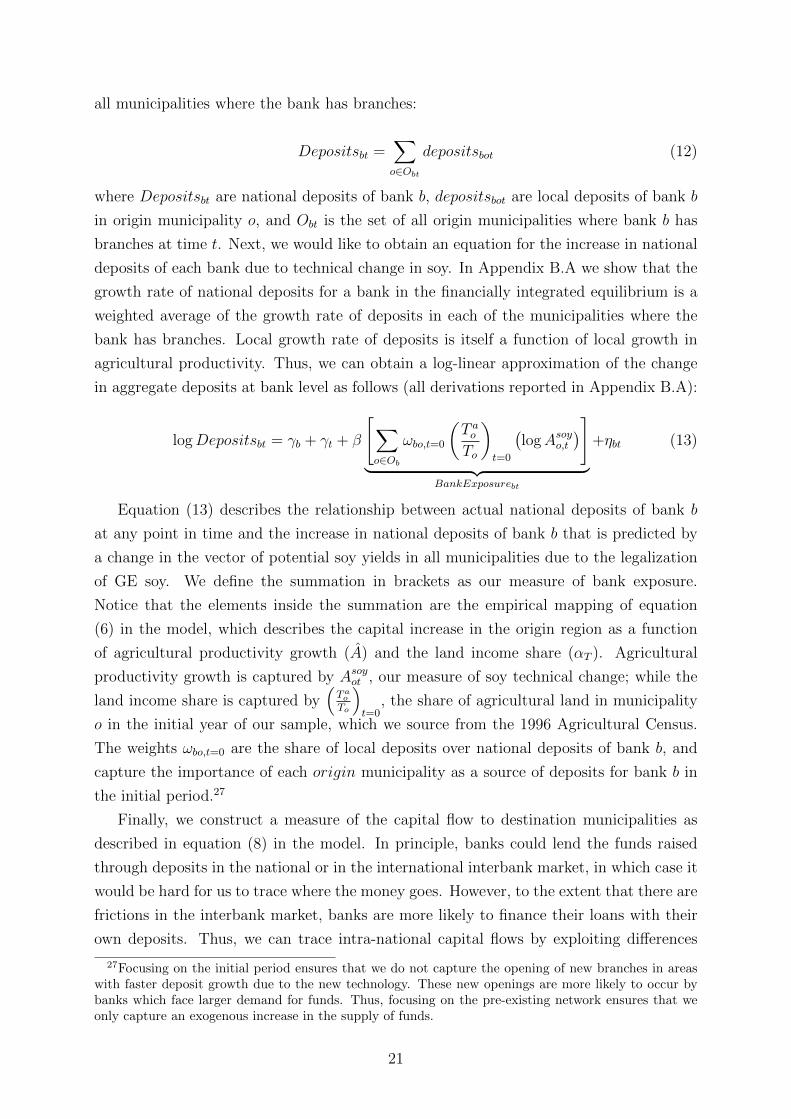
Depositsbt =∑o∈Obt

depositsbot (12)

where Depositsbt are national deposits of bank b, depositsbot are local deposits of bank b

in origin municipality o, and Obt is the set of all origin municipalities where bank b has

branches at time t. Next, we would like to obtain an equation for the increase in national

deposits of each bank due to technical change in soy. In Appendix B.A we show that the

growth rate of national deposits for a bank in the financially integrated equilibrium is a

weighted average of the growth rate of deposits in each of the municipalities where the

bank has branches. Local growth rate of deposits is itself a function of local growth in

agricultural productivity. Thus, we can obtain a log-linear approximation of the change

in aggregate deposits at bank level as follows (all derivations reported in Appendix B.A):

logDepositsbt = γb + γt + β

[∑o∈Ob

ωbo,t=0

(T aoTo

)t=0

(logAsoyo,t

)]︸ ︷︷ ︸

BankExposurebt

+ηbt (13)

Equation (13) describes the relationship between actual national deposits of bank b

at any point in time and the increase in national deposits of bank b that is predicted by

a change in the vector of potential soy yields in all municipalities due to the legalization

of GE soy. We define the summation in brackets as our measure of bank exposure.

Notice that the elements inside the summation are the empirical mapping of equation

(6) in the model, which describes the capital increase in the origin region as a function

of agricultural productivity growth (A) and the land income share (αT ). Agricultural

productivity growth is captured by Asoyot , our measure of soy technical change; while the

land income share is captured by(Tao

To

)t=0

, the share of agricultural land in municipality

o in the initial year of our sample, which we source from the 1996 Agricultural Census.

The weights ωbo,t=0 are the share of local deposits over national deposits of bank b, and

capture the importance of each origin municipality as a source of deposits for bank b in

the initial period.27

Finally, we construct a measure of the capital flow to destination municipalities as

described in equation (8) in the model. In principle, banks could lend the funds raised

through deposits in the national or in the international interbank market, in which case it

would be hard for us to trace where the money goes. However, to the extent that there are

frictions in the interbank market, banks are more likely to finance their loans with their

own deposits. Thus, we can trace intra-national capital flows by exploiting differences

27Focusing on the initial period ensures that we do not capture the opening of new branches in areaswith faster deposit growth due to the new technology. These new openings are more likely to occur bybanks which face larger demand for funds. Thus, focusing on the pre-existing network ensures that weonly capture an exogenous increase in the supply of funds.

21

in the geographical structure of bank branch networks. To do this, we make the simple

assumption that each bank responds to the growth in deposits by increasing the supply of

funds proportionally in all municipalities where it has branches. Using this assumption,

in Appendix B.A we show that the growth of credit in each destination municipality

can be written as a weighted average of the growth rate of national deposits in each bank

present in that destination municipality, which in turn is a weighted average of agricultural

productivity growth in each origin municipality where the bank has branches.28 The

empirical counterpart of this measure of destination municipality exposure can be written

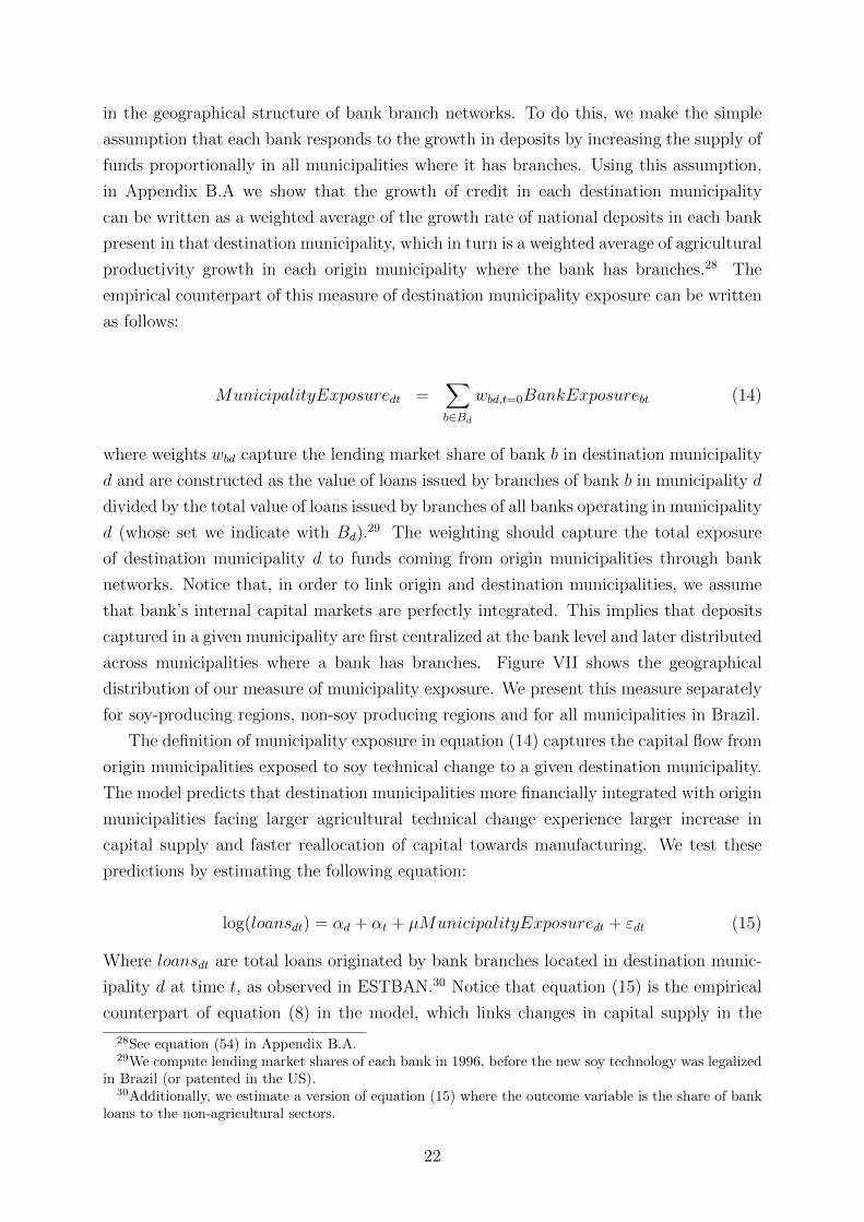
as follows:

MunicipalityExposuredt =∑b∈Bd

wbd,t=0BankExposurebt (14)

where weights wbd capture the lending market share of bank b in destination municipality

d and are constructed as the value of loans issued by branches of bank b in municipality d

divided by the total value of loans issued by branches of all banks operating in municipality

d (whose set we indicate with Bd).29 The weighting should capture the total exposure

of destination municipality d to funds coming from origin municipalities through bank

networks. Notice that, in order to link origin and destination municipalities, we assume

that bank’s internal capital markets are perfectly integrated. This implies that deposits

captured in a given municipality are first centralized at the bank level and later distributed

across municipalities where a bank has branches. Figure VII shows the geographical

distribution of our measure of municipality exposure. We present this measure separately

for soy-producing regions, non-soy producing regions and for all municipalities in Brazil.

The definition of municipality exposure in equation (14) captures the capital flow from

origin municipalities exposed to soy technical change to a given destination municipality.

The model predicts that destination municipalities more financially integrated with origin

municipalities facing larger agricultural technical change experience larger increase in

capital supply and faster reallocation of capital towards manufacturing. We test these

predictions by estimating the following equation:

log(loansdt) = αd + αt + µMunicipalityExposuredt + εdt (15)

Where loansdt are total loans originated by bank branches located in destination munic-

ipality d at time t, as observed in ESTBAN.30 Notice that equation (15) is the empirical

counterpart of equation (8) in the model, which links changes in capital supply in the

28See equation (54) in Appendix B.A.29We compute lending market shares of each bank in 1996, before the new soy technology was legalized

in Brazil (or patented in the US).30Additionally, we estimate a version of equation (15) where the outcome variable is the share of bank

loans to the non-agricultural sectors.

22

destination region with capital outflows from the origin region.31 Appendix B.B reports

the derivations to obtain equation (15).

III.C Capital reallocation towards destination firms: Data and Empiri-

cal Strategy

A potential concern with the identification strategy described in subsection III.B is

that destination municipalities that are more financially connected to origin municipalities

might also be more connected through migration or commercial networks. In that case,

our estimates could be capturing the effects of agricultural technical change in origin

municipalities on bank lending in destination municipalities through a labor supply or a

demand channel, rather than the capital supply mechanism described in the model. To

make progress on this front, we bring our analysis at a more micro-level and trace the

reallocation of capital towards firms located in destination municipalities.

In particular, we construct a measure of firm-level exposure to capital inflows from ori-

gin municipalities using information on pre-existing firm-bank relationships. To construct

this measure we match administrative data on the credit and employment relationships

for the universe of formal firms operating in Brazil. Data on credit relationships between

firms and financial institutions is sourced from the Credit Information System of the Cen-

tral Bank of Brazil for the years 1997 to 2010.32 The confidential version of the Credit

Information System uniquely identifies both the lender (bank) and the borrower (firm) in

each credit relationship. This allows us to match data on bank-firm credit relationships

with data on firm characteristics from the Annual Social Information System (RAIS).

RAIS is an employer-employee dataset that provides individual information on all formal

workers in Brazil.33 Using worker level data, we constructed the following set of variables

at firm-level: employment, wage bill, sector of operation and geographical location.34 One

31As can be seen by replacing equations (6) and (7) into equation (8) in the model, capital outflows inthe origin region are a function of agricultural technical change (A). Thus, equation (15) is effectively areduced form version of the relationship described by equation (8) in the model.

32The Credit Information System and ESTBAN are confidential datasets of the Central Bank of Brazil.The collection and manipulation of individual loan-level data and bank-branch data were conductedexclusively by the staff of the Central Bank of Brazil.The dataset reports a set of loan and borrowercharacteristics, including loan amount, type of loan and repayment performance. We focus on totaloutstanding loan amount, which refers to the actual use of credit lines. In this sense, our definition ofaccess to bank finance refers to the actual use and not to the potential available credit lines of firms.Unfortunately, data on interest rate is only available from 2004, after GE soy legalization.

33Employers are required by law to provide detailed worker information to the Ministry of Labor.See Decree n. 76.900, December 23rd 1975. Failure to report can result in fines. RAIS is used by theBrazilian Ministry of Labor to identify workers entitled to unemployment benefits (Seguro Desemprego)and federal wage supplement program (Abono Salarial). For firms with ten or more employees, RAIScovers, on average, 76.2 percent of firms with a juridical person fiscal code that are present in the BrazilianBusiness Registry (CEMPRE) during the period under study. It is important to notice that our data onbank-firm relationships exclusively covers the formal sector, as firms need to have a tax identifier (CNPJ)to apply for a loan and need to make contributions to the social security system in order to be registeredin the employer-employee datasets (RAIS).

34When a firm has multiple plants, we aggregate information on employment and wage bill across

23

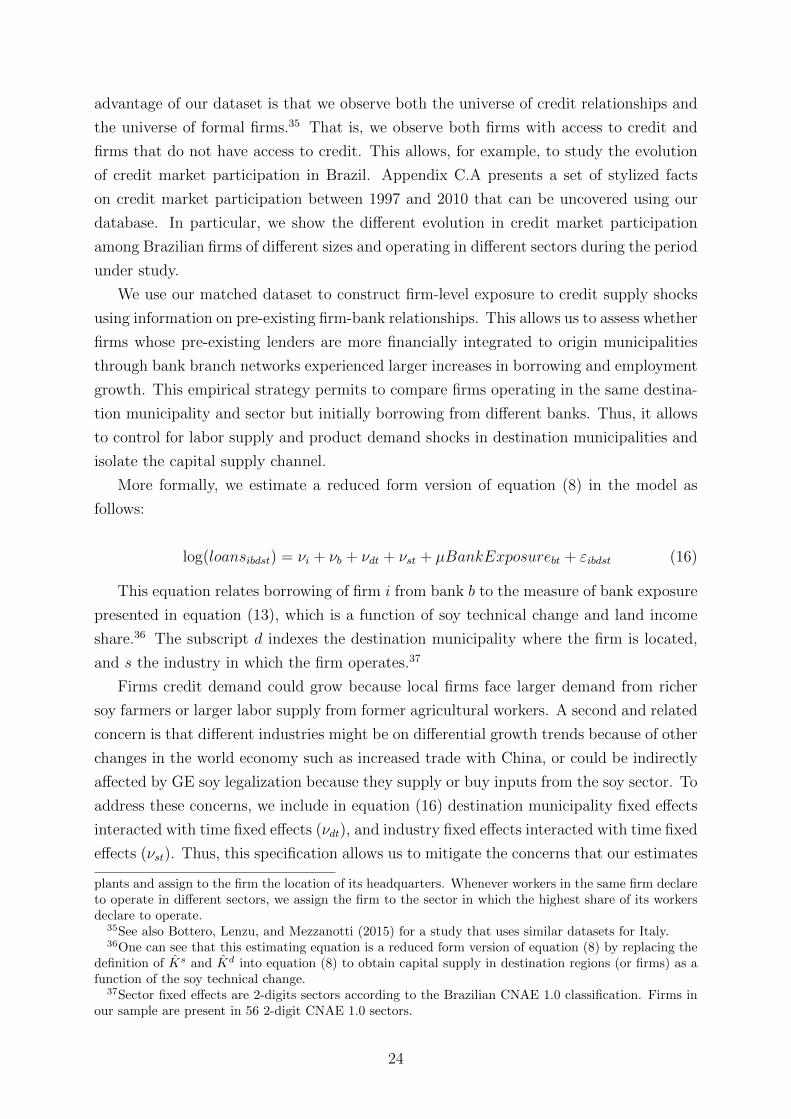
advantage of our dataset is that we observe both the universe of credit relationships and

the universe of formal firms.35 That is, we observe both firms with access to credit and

firms that do not have access to credit. This allows, for example, to study the evolution

of credit market participation in Brazil. Appendix C.A presents a set of stylized facts

on credit market participation between 1997 and 2010 that can be uncovered using our

database. In particular, we show the different evolution in credit market participation

among Brazilian firms of different sizes and operating in different sectors during the period

under study.

We use our matched dataset to construct firm-level exposure to credit supply shocks

using information on pre-existing firm-bank relationships. This allows us to assess whether

firms whose pre-existing lenders are more financially integrated to origin municipalities

through bank branch networks experienced larger increases in borrowing and employment

growth. This empirical strategy permits to compare firms operating in the same destina-

tion municipality and sector but initially borrowing from different banks. Thus, it allows

to control for labor supply and product demand shocks in destination municipalities and

isolate the capital supply channel.

More formally, we estimate a reduced form version of equation (8) in the model as

follows:

log(loansibdst) = νi + νb + νdt + νst + µBankExposurebt + εibdst (16)

This equation relates borrowing of firm i from bank b to the measure of bank exposure

presented in equation (13), which is a function of soy technical change and land income

share.36 The subscript d indexes the destination municipality where the firm is located,

and s the industry in which the firm operates.37

Firms credit demand could grow because local firms face larger demand from richer

soy farmers or larger labor supply from former agricultural workers. A second and related

concern is that different industries might be on differential growth trends because of other

changes in the world economy such as increased trade with China, or could be indirectly

affected by GE soy legalization because they supply or buy inputs from the soy sector. To

address these concerns, we include in equation (16) destination municipality fixed effects

interacted with time fixed effects (νdt), and industry fixed effects interacted with time fixed

effects (νst). Thus, this specification allows us to mitigate the concerns that our estimates

plants and assign to the firm the location of its headquarters. Whenever workers in the same firm declareto operate in different sectors, we assign the firm to the sector in which the highest share of its workersdeclare to operate.

35See also Bottero, Lenzu, and Mezzanotti (2015) for a study that uses similar datasets for Italy.36One can see that this estimating equation is a reduced form version of equation (8) by replacing the

definition of Ks and Kd into equation (8) to obtain capital supply in destination regions (or firms) as afunction of the soy technical change.

37Sector fixed effects are 2-digits sectors according to the Brazilian CNAE 1.0 classification. Firms inour sample are present in 56 2-digit CNAE 1.0 sectors.

24

could be capturing the effects of agricultural technical change in origin municipalities on

bank lending in destination municipalities through a labor supply or a demand channel,

rather than the capital supply mechanism described in the model.38

In addition to study the effect of capital reallocation on firm borrowing, we are also

interested in assessing its real effects. In particular, we want to understand the extent

to which firms use additional credit to finance growth enhancing investments. These

investments can take the form of expanding the use of capital, labor or other inputs.

Because in the RAIS dataset we observe labor and the wage bill, we focus our analysis

on these two inputs. However, to the extent that there is some complementarity between

production inputs, we expect that any investment leading to expansion of the firm is likely

to be reflected in larger employment and wage bill. Thus, we analyze real effects through

the following firm-level specification:

log(Lidst) = νi + νdt + νst + λFirmExposureit + εidst (17)

where:

FirmExposureit =∑b∈B

πib,t=0 BankExposurebt

The variable Lidst denotes employment in firm i, located in destination municipality d,

operating in industry s at time t,. Our measure of firm exposure is defined as a weighted

average of bank exposure of all lenders with which firm i had a credit relationship in the

pre GE-soy legalization period, which correspond to the years 2001 and 2002 in the Credit

Registry Data. The weights πib,t=0 correspond to the share of borrowing of firm i from

bank b in 2001 and 2002 as a share of total borrowing of firm i in the same years. We

use pre-existing bank relationships to minimize the concern that endogenous formation

of firm-bank relationships — which could depend from a bank exposure to the soy boom

— might affect our results.39

IV Local Effects of Soy Technical Change

We start by estimating the effect of local agricultural technical change on local land

rents. In both the autarky and financial integration equilibrium, the model predicts that

municipalities experiencing faster technical change should experience faster growth in land

38All our results are robust to restricting our sample to firms operating in non-soy producing munici-palities (that is, municipalities that do not produce soy at any point during the period under study) andfirms not operating in sectors directly linked to soy production through input-output linkages. Theseresults are available from the authors upon request.

39Notice that this implies that we use the exposure of the pre-2003 lenders for all years in which a firmis present in our sample, no matter whether the firm is borrowing or not from those lenders in the yearsafter GE soy legalization. Since the set of lenders used to construct this measure is defined in the initialperiod and it is constant for each firm, the bank fixed effects νb are effectively absorbed by firm fixedeffects νi in this specification.

25

rents, as described in equations (1) and (5) where land cost shares in agricultural and

manufacturing production (θTA and θTM) are the same for all municipalities due to factor

price equalization in the benchmark equilibrium and γ is a parameter measuring the degree

of persistence of the increase in agricultural profitability. As described in section III.A,

we proxy for land rents with agricultural profits sourced from the Agricultural Census of

Brazil. Data is collected through direct interviews with the managers of each agricultural

establishment and it is available aggregated at municipality level. Since the Agricultural

Census is released at intervals of 10 years, we focus on the last two waves (1996 and 2006)

and estimate the following first-difference version of equation (10):

∆yj = ∆α + β∆ log(Asoyj ) + ∆εj (18)

Where ∆yj is the decadal change in outcome variables between 1996 and 2006 and

∆ log(Asoyj ) = log(Asoy,HIGHj )− log(Asoy,LOWj ).

Columns 1 and 2 of Table II show the results of estimating equation (18) when the

outcome is agricultural profits per hectare.40 The point estimate on ∆ log(Asoyjt ) indicates

that municipalities with a one standard deviation larger increase in soy technical change

experienced a 10.7 percent larger increase in agricultural profits per hectare between 1996

and 2006. In principle, extra agricultural profits could have been reinvested in agricul-

ture, channeled into consumption, or into savings. We start by studying the effect of soy

technical change on agricultural investment in columns 3 and 4 of Table II. The estimated

coefficient on ∆ log(Asoyjt ) is positive and significant, indicating the municipalities more

exposed to soy technical change experienced larger increase in investment in agriculture.

The magnitude of the estimated coefficient in column (4) is similar to the effect on agri-

cultural profits per hectare. However, agricultural profits per hectare are three times

larger than investment per hectare in the 1996 Agricultural Census baseline. Thus, taken

together, these coefficients imply that for every R$10 increase in profits per hectare due

to soy technical change, only around R$3.45 are reinvested in agricultural activities.

Next, we estimate the effect of local agricultural technical change on local savings. In

both the autarky and financial integration equilibrium, the model predicts that munic-

ipalities experiencing faster technical change should experience faster growth in capital

supply, as described in equations (3) and (6) where land cost shares (θTA and θTM) are

the same for all municipalities but the land income share (αT ) varies across municipalities

depending on their land and capital endowments. To test this prediction, we estimate

equation (10) where the outcome variable is the log of the total value of bank deposits

in bank branches located in municipality j.41 We define bank deposits as the sum of

40Using a similar identification strategy, Bustos et al. (2016) show that municipalities more exposed tosoy technical change experienced higher adoption of GE soy seeds and higher agricultural productivitygrowth in the period between 1996 and 2006. We replicate these results for the sample of municipalitiesstudied in this paper in Table C1 of the Appendix.

41Notice that when estimating equation (10) we focus on the average effects of soy technical change on

26

deposits in checking accounts, saving accounts and term deposits.42 Results are reported

in columns 1 and 2 of Table III. The estimates indicate that municipalities with higher

increase in soy technical change experienced a larger increase in local bank deposits during

the period under study. The magnitude of the estimated coefficient in column 2 indicates

that a municipality with a one standard deviation higher increase in soy technical change

experienced a 8 percent larger increase in bank deposits in local branches.43

We also investigate the timing of the effect of soy technical change on bank deposits,

and in particular whether it is consistent with the legalization of GE soy seeds in 2003. To

this end, we estimate a version of equation (10) in which we allow the effect of ∆ log(Asoyj )

to vary over time. Figure VIII plots the time varying estimated coefficients on ∆ log(Asoyj )

and ninety-nine-percent confidence intervals when the outcome variable is the log of de-

posits in local bank branches.44 As shown, the timing of the effect is consistent with the

timing of the legalization of GE soy seeds. There are no pre-existing trends in the years

1996 to 2001 – the magnitude of the point estimates is close to zero and not statistically

significant – and positive effects of soy technical change on local deposits afterwards.45

We find, however, that the effect starts in 2002, one year before the official legalization

of GE soy seeds. This is consistent with the timing of the expansion in the area planted

with soy documented in Figure IV. This figure documents a break in the trend of the

expansion of the area area planted with soy in 2002 when GE soy seeds were smuggled

from Argentina (USDA 2001).

In the case of financial integration, our model predicts that municipalities with faster

agricultural productivity growth experience capital outflows if the capital supply effect is

deposits. That is, we do not take into account the heterogeneous effects predicted by the model dependingon the land income share in each municipalities. This is to keep these results directly comparable withthose on agricultural outcomes presented in Table II. We will take into account differences in land incomeshares across municipalities when computing our measure of bank exposure in the next step.

42Data on bank outcomes is sourced from the ESTBAN dataset, which has detailed information onbalance sheet and location of branches of all commercial banks operating in Brazil. As such, our analysisin this section focuses on municipalities with at least one bank branch. During the period under studywe have data on bank branches located in 3154 AMCs (75 percent of all Brazilian AMCs).

43In additional results reported in Table C2 of Appendix C, we decompose the effect of soy technicalchange on deposits into three different types: checking, savings and term deposits accounts. One potentialconcern is that areas more affected by the soy boom experienced an increase in the use of formal bankingdue to the higher amount of transactions linked to growing soy production rather than an increase inactual savings. As shown in Table C2, the growth in deposits triggered by soy technical change wasconcentrated in saving deposits.

44These estimated coefficients are net of municipality controls interacted with time fixed effects as incolumn 2 of Table III.

45These results also imply that our estimates do not capture a delayed response to the trade liberal-ization that occurred at the beginning of the previous decade in areas with different initial agriculturalintensity, as studied by Dix-Carneiro and Kovak (2017). In particular, Dix-Carneiro and Kovak (2017)find long-run negative effects of tariff cuts on formal employment and earnings and show that tariff cutswere smaller in the agricultural sector relative to other sectors. By showing that soy technical change hasno effect on bank deposits until the early 2000s, Figure VIII addresses the concern that the long-liveddynamics of the trade liberalization of the early 1990s has a confounding effect on our results.

27

larger than the capital demand effect.46 To test this prediction, we estimate equation (10)

when the outcome variable is the total value of loans originated by bank branches located

in municipality j.47 The results are reported in columns 3 and 4 of Table III and show

that municipalities with higher increase in soy technical change experienced a decrease in

bank loans originated by local branches. Taken together, the results reported in columns 2

and 4 suggest that municipalities that experienced larger increase in soy technical change

experience an increase in deposits and a decrease in loans, thus becoming net exporters

of capital. To test the model prediction more formally, in columns 5 and 6 of Table

III we estimate equation (10) when the outcome variable is capital outflow, defined as

total value of deposits minus total value of loans originated by bank branches located in

municipality j, divided by total assets of the same branches. As shown, we find a positive

and precisely estimated coefficient on log(Asoyj ), which indicates that municipalities with

higher increase in soy technical change experienced a larger net increase in capital export

through the formal banking sector during the period under study.

V Capital reallocation towards destination municipalities

The results presented in section IV show that the adoption of new agricultural tech-

nologies in soy production generates more profits than investments in the agricultural sec-

tor, as well as capital outflows from origin municipalities. This suggests that the capital

supply effect dominates the capital demand effect. In this case, our theoretical framework

predicts that destination municipalities financially integrated with origin municipalities

facing larger agricultural technical change should experience both larger capital inflows

and faster reallocation of capital towards manufacturing.

In this section we test these predictions using the specification presented in equation

(15). We focus on two main outcome variables: total bank lending and the share of bank

lending to non-agricultural sectors in destination municipalities. These two outcomes

capture, respectively, capital inflows and capital reallocation towards manufacturing in the

model. Table IV reports the results. We find that municipalities with a larger exposure to

the soy-driven deposit increase experienced a larger increase in bank lending. Recall from

the discussion in section III.B that our measure of municipality exposure is a (weighted)

46This is because municipalities with a larger increase in agricultural productivity face a larger increasein land rents and, as a result, a larger increase in the capital intensity of the agricultural sector and alarger reallocation of capital towards agriculture. Still, if the growth in capital supply is larger than thegrowth in capital demand, they face capital outflows.

47Notice that the total value of loans includes loans to both individuals and firms, which we cannotseparate in ESTBAN. We observe three major categories of bank loans: rural loans, which includes loansto the agricultural sector; general purpose loans to firms and individuals, which includes: current accountoverdrafts, personal loans, accounts receivable financing and special financing for micro-enterprises amongothers; and specific purpose loans which includes loans with a specific objective, such as export financing,or acquisition of vehicles.The ESTBAN data do not allow us to distinguish between loans to individualsand loans to firms. Also, we can not distinguish loans to different sectors with the exception of ruralloans, which are loans directed to individuals or firms operating in the agricultural sector.

28

average of the GE-soy driven national deposit growth of the banks operating in a given

municipality. This implies that a destination municipality with a standard deviation

higher exposure is a municipality whose banks experienced, on average, a 2.3 percentage

points faster annual growth in national deposits due to soy technical change in the post-GE

soy legalization period.48 The magnitude of the estimated coefficient reported in column

(1) of Table IV indicates that a municipality whose banks experienced a 2.3 percentage

points annual growth in deposits due to soy technical change experienced a 0.4 percentage

points faster annual growth in bank lending in the post-GE soy legalization period.49

Next, in columns 2 and 3, we split the sample in soy-producing and non-soy producing

municipalities.50 Each of these groups accounts for around half of the observations used in

column 1. The estimated coefficient in the soy-producing sample is positive but small in

size (0.054) and not statistically significant, while the estimated coefficient on the non-soy

producing sample is 0.580 and strongly significant. These results indicate a reallocation

of capital towards non-soy producing regions, as predicted by the model when the capital

supply effect is larger than the capital demand effect in soy producing regions.

We then study whether this increase in lending has been directed towards agricultural

or non-agricultural sectors. Since rural loans are observable in the ESTBAN dataset, we

can construct as outcome variable the share of bank lending to sectors other than agricul-

ture. As shown in column (4) we find that municipalities more financially integrated with

soy producing regions experienced a larger increase in non-agricultural lending as a share

of total lending (1.7 percentage points for a standard deviation difference in municipality

exposure). This effect is present in both soy-producing and non soy-producing regions,

although largely concentrated in the latter (see columns 5 and 6).

The findings discussed above are consistent with the capital supply mechanism empha-

sized by the model: agricultural technical change can increase savings in soy-producing

regions and lead to capital outflows towards non-soy producing regions where capital

reallocates towards the capital intensive sector, manufacturing. Our empirical analysis

permits to quantify this effect by comparing the speed of capital reallocation across sectors

48A standard deviation in the increase in municipality exposure across municipalities between theperiod before and the period after GE soy legalization is 0.18. To obtain the average annual growthwe divide this number by the number of years in the post-GE soy legalization period for which data isavailable (2003-2010). Notice also that the average annual growth rate of bank deposits across Brazilianmunicipalities in the post-GE soy legalization period was 10 percent.

49To obtain this annualized growth in lending we multiply a standard deviation in the increase in munic-ipality exposure across municipalities between the period before and the period after GE soy legalization(0.18) by the elasticity of loan growth to deposit growth γ (see equation (54) in Appendix B.A). As shownin Appendix B.B, the elasticity of loan growth to deposit growth (γ) can be obtained by dividing thecoefficient µ in equation (15) by the coefficient β in equation (13). This is because µ = γβ. Empirically,we calculate γ by dividing the estimated coefficient in column (1) of Table IV by the estimated coefficientin column (4) of Table V. Table V studies the relationship between national deposits of bank b and theincrease in aggregate deposits for the same bank that is predicted by our measure of bank exposure.

50Non-soy producing municipalities are those with no agricultural area farmed with soy at any pointin time between 1996 and 2010.

29

in non-soy producing municipalities with different degrees of financial integration with the

soy boom area. During the period under study (1996-2010), the share of non-agricultural

lending increased from 74.6 to 83.5 percent in the average non-soy producing municipal-

ity. However, the degree of capital reallocation away from agriculture varied extensively

across municipalities: the interquartile range was 22 percentage points. Our estimates im-

ply that the differences in the degree of financial integration with the soy boom area can

explain 11 percent of the observed differences in the increase in non-agricultural lending

share across non-soy producing municipalities.51

Overall, the results presented in Table IV are consistent with the predictions of the

model and indicate that new agricultural technologies can generate structural transforma-

tion in regions not directly affected by such technologies. Two caveats with this specifica-

tion are in order. First, this specification does not allow us to distinguish the direct effect

of capital reallocation from the labor supply or product demand channels of agricultural

productivity growth. For example, destination municipalities served by more exposed

banks might also be better connected to soy-producing regions through transportation or

migrant networks. Therefore, in section III.C, we propose an identification strategy that

aims at identifying the capital supply channel separately from other channels using loan-

level and firm-level data. Second, the ESTBAN dataset used to construct the agricultural

and non-agricultural lending shares used as outcomes in this section includes lending to

both firms and individuals. This has the advantage of capturing loans to farmers who take

personal loans to invest in their farm, but the disadvantage of also including mortgages

and other personal consumption loans. Therefore, in section VI, we use loan-level data

to more precisely identify credit flows to firms in different sectors.

VI Capital reallocation towards destination firms

In section IV we showed that regions more affected by technical change in soy pro-

duction experience capital outflows. In section V we showed that regions that are more

financially integrated with soy producing regions through the bank network experience a

larger increase in non-agricultural lending. In this section we bring the analysis at the firm

level through the identification strategy proposed in section III.C and study how increases

in bank deposits due to soy technical change affected capital supply to firms in destination

municipalities. We proceed as follows. First, we document that our measure of bank ex-

posure predicts aggregate deposit growth at the bank level. Next, we study whether firms

that are more financially integrated with origin municipalities through their pre-existing

banking relationships experienced larger growth in borrowing and employment.

51That is, one standard deviation in our measure of municipality exposure explains 11 percent of astandard deviation in the increase in non-agricultural lending share across non-soy producing municipal-ities.

30

VI.A Bank exposure and aggregate deposits

We start by testing the relationship between aggregate deposits of bank b and the

increase in aggregate deposits for the same bank that is predicted by our measure of

bank exposure. Table V reports the results of estimating equation (13) when the out-

come variable is aggregate deposits of bank b, and bank-year observations are weighted

by initial bank size.52 Aggregate deposits for each bank are obtained summing branch

level deposits from ESTBAN.53 The point estimate on BankExposure is positive and sig-

nificant, which indicates that banks more exposed to soy technical change through their

branch network experienced higher increase in aggregate deposits. The magnitude of the

estimated coefficient reported in column 1 is 1.42. It indicates that a 1 percent increase in

aggregate deposits of bank b predicted by the change in the vector of potential soy yields

correspond to a 1.42 percent increase in actual national deposits of the same bank. In

other words, changes in our measure of predicted deposits are associated with changes in

actual deposits of similar magnitude.54 Columns 2 to 4 show that this effect is not driven

by differential growth trends across banks of different initial size or deposit-to-asset ratio.

Finally, in Figures IX (a) and (b) we report partial correlations between changes in bank

exposure and changes in the log of aggregate deposits at bank level, weighting and with-

out weighting by initial bank size respectively.55 As shown, our estimates are not driven

by extreme observations or weighting by bank size.

VI.B Bank-firm level specification

In this section we study the effect of bank exposure on firm borrowing from that same

bank.56 Table VI shows the results of estimating equation (16) described in section III.C

when the outcome variable is the log of the monetary value of outstanding loan balance

of firm i from bank b.

We start by estimating equation (16) in a specification with firm, bank and time fixed

52As captured by bank assets in the initial year. Our results do not depend on this weighting, as shownin Figure IX.

53We focus on the years 2001 to 2010 in order to match the same time period used in the firm-levelanalysis presented in the next subsections.

54We think that one reason why our estimate of β is larger than one is that our measure of Bankexposure is a first order approximation to changes in aggregate deposits holding the bank branch networkconstant. Thus, changes in the bank branch network are in the error term. It is very likely that the soyboom might have led banks to open new branches which capture deposits. Thus, our measure of bankexposure might underestimate the effect of the soy shock on aggregate deposits.

55This is equivalent to a first difference version of equation (13) obtained after partialling out year fixedeffects and bank initial characteristics interacted with linear time trends and then averaging bank exposureand log deposits for each bank in the years before (2001-2002) and after (2003-2010) the legalization ofGE soy seeds.

56In order to minimize sample selection, we focus our analysis at firm-level on the period 2001-2010,i.e. the years after the reporting threshold of the Credit Registry was lowered to 5,000 BRL. As shown inFigure C.1 of the Appendix, in 2001 only around 7 percent of Brazilian firms had access to finance whenusing the 50,000 BRL reporting threshold. In the same year, 31 percent of Brazilian firms had access tofinance under the 5,000 BRL reporting threshold.

31

effects in column 1. The estimated coefficient on the variable BankExposure is positive,

indicating that firms with pre-existing relationships with more exposed banks experienced

a larger increase in borrowing from those banks. In column 2 we add municipality and

sector fixed effects, both interacted with time fixed effects. Notice that we find similar

point estimates when controlling for municipality and sector-level shocks, which should

capture any labor supply or product demand effects across firms in the same location.

This suggests that the increase in firm borrowing is driven by the capital supply effect of

agricultural technical change.

Similarly to the destination municipality results presented in section V, we can quantify

the effect on firm borrowing for a given increase in bank deposits. First, notice that the

coefficients on bank exposure presented in Table VI are of similar magnitude of those on

municipality exposure presented in Table IV when the outcome was total bank lending in

a given municipality. In particular, the estimated coefficient in column (2) indicates that

firms with a pre-existing relationship with a bank experiencing a 2.3 percentage points

faster deposit growth due to soy technical change experienced a 0.4 percentage points

faster annual growth in borrowing in the post-GE soy legalization period. The similarity

in point estimates between Table IV and Table VI also implies that our municipality level

measure of total bank lending well captures bank lending to firms, and that our effects

are driven by the intensive rather than the extensive margin of bank lending.

In column 4 we augment equation (16) with firm fixed effects interacted with time

fixed effects. This specification fully captures firm-specific demand shocks, and only

exploits variation across banking relationships within firm to identify the coefficient on

bank exposure (Khwaja and Mian 2008). As a consequence, it can only be estimated

using firms with multiple lending relationships in both the pre and the post GE soy

legalization period. The estimated coefficient is positive, which implies that banks with

larger exposure to the soy-driven deposit shock increased their lending by more to the

same firm. Notice also that the magnitude of the estimated coefficient is similar to the

one obtained without firm-time fixed effect on the same sample of firms. This indicates

that the effect of bank exposure on firm borrowing is driven by credit supply forces rather

than unobservable firm-specific demand shocks correlated with lender exposure.57

Next, we study the effect of bank exposure on loans by sector of operation of the

borrowing firm. To this end, we estimate equation (16) separately for borrowers operating

in agriculture, manufacturing, services, and other sectors.58 Table VII reports the results.

57Under certain assumptions regarding the functional form of the underlying model describing borrow-ing of firm i from bank b, the difference in point estimates between specifications that include firm fixedeffects and those that do not captures the size of the bias induced by endogenous matching between firmsand banks (see Khwaja and Mian 2008).

58Services include: construction, commerce, lodging and restaurants, transport, housing services, do-mestic workers and other personal services. We exclude banks and other firms in the financial sector.Other sectors include: public administration, education, health, international organizations, extraction,and public utilities.

32

We find positive coefficients for firms in all sectors. The effects are precisely estimated for

firms in manufacturing and services, while not statistically significant for agriculture and

other sectors. The magnitude of the estimated coefficients is largest in the manufacturing

sector (0.304) and smallest in the agricultural sector (0.204). These magnitudes imply

that a standard deviation difference in GE-soy driven deposit growth – which corresponds

to a 3.4 percentage points faster annual growth in the post-GE legalization period –

translates into 2.2 percentage points faster annual growth in borrowing for firms operating

in manufacturing, 2 percentage points for firms operating in services, 1.6 percentage

points for firms operating in other sectors and 1.5 percentage points for firms operating

in agriculture. Taking into account differences in average loan size and number of loans

across sectors in the pre GE-soy legalization period, these estimates indicate that out of 1

R$ of new loans in destination municipalities from the soy-driven deposit shock, 1.3 cents

were allocated to firms in agriculture, 50 cents to firms in manufacturing, 39.7 cents to

firms in services and 9 cents to firms in other sectors.59

To sum up, in this section we show that firms more financially integrated with ori-

gin municipalities through their pre-existing banking relationships experienced a larger

increase in borrowing from those banks. Second, capital flowing from origin to destina-

tion municipalities due to soy technical change was mostly allocated to firms operating

in the non-agricultural sectors (manufacturing and services). These findings are obtained

exploiting variation across firms within destination municipalities, and support the in-

terpretation of the municipality-level results presented in section V as resulting from the

capital supply channel.

VI.C Firm level specification: real effects

Finally, we study the effect of firm exposure to soy technical change through pre-

existing bank relationships on firm growth. To this end, we estimate equation (17) as

described in section III.C. We focus on two main outcome variables: employment, defined

as the log of the yearly average number of workers; and wage bill, defined as the log of

the monetary value of the firm total wage bill.

The results are reported in Table VIII. We find positive real effects on firm size. Firms

whose pre-existing lenders have a larger exposure to the soy-driven deposit increase expe-

rienced a larger growth in employment and wage bill. In contrast with the loan estimates

discussed in subsection VI.B, we find that our estimated real effects decrease in magnitude

59This quantification is obtained as follows. First, we multiply the estimated coefficient on bankexposure by the average loan size in the years 2001 and 2002 in each sector. This gives us the estimatedincrease in loan size for the average loan in each sector, in response to a unit increase in exposure ofthe main lender of the borrower. Second, we multiply this estimate by the average number of loans tofirms operating in each sector in the years 2001 and 2002. This multiplication gives us an estimate ofthe total increase in the value of loans of firms in each sector in response to a unit increase in exposureof their lenders. Finally, we use these estimates of total increase in loan value in each sector to computethe allocation across-sectors of 1 R$ of new loans from the soy-driven deposit shock.

33

when we control for municipality and sector-level shocks. This can be seen, for example,

by comparing columns 1 and 2 in Table VIII. The coefficient on firm exposure when the

outcome is employment goes from 0.269 to 0.159 when adding municipality and sector

fixed effects interacted with year fixed effects. This finding indicates that municipalities

more connected through bank branch networks might also be more connected through

transportation or commercial networks, thus are more likely to receive not only capi-

tal supply shocks but also labor supply and product demand shocks due to agricultural

productivity growth.

Next, we estimate the same equation by sector of operation of each firm. Table IX

reports the results. As shown, the average effects of firm exposure on firm size are pos-

itive and similar in size in agriculture, manufacturing and services, while small and not

statistically significant for firms operating in other sectors. These estimates, along with

differences in average firm size and number of firms in each sector, can be used to com-

pute the allocation of extra workers across sectors for a given increase in firm exposure.

Our estimated coefficients indicate that out of 100 additional workers in destination mu-

nicipalities due to the soy-driven deposit shock, 2 were employed in agriculture, 40 in

manufacturing, 54 in services and 4 in other sectors. To sum up, our results indicate that

reallocation of capital from origin to destination municipalities had real effects on em-

ployment, and these effects were concentrated in the manufacturing and services sectors.

VII Concluding Remarks

This paper studies the effect of agricultural productivity on structural transformation

in open economies through its impact on capital accumulation. The empirical analysis

is focused on the widespread adoption of genetically engineered soy in Brazil. This new

technology allows farmers to obtain the same yield with lower production costs, thus in-

creasing agricultural profits. The effect of the new agricultural technology on structural

transformation via capital accumulation depends on several features of the environment.

First, the relative strength of the demand and supply effects of agricultural technical

change, which, as highlighted in our model, work in opposite directions. The finding that

the adoption of genetically engineered soy seeds generated more profits than investment

in agriculture suggests that the supply effect dominates. Indeed, we find a positive effect

of GE soy adoption on deposits in local bank branches. In this case, the model predicts

that capital reallocates towards non-agricultural sectors. Because in our setting soy pro-

ducing regions tend to be rural, this reallocation needs to take place both across sectors

and regions. Indeed, branches located in soy producing areas were net capital exporters,

and capital reallocated towards non-soy producing regions. Thus, a second key feature of

the environment is the degree of financial integration across regions. We find that regions

more financially integrated with the soy boom area experience faster structural transfor-

34

mation. In particular, banks experiencing faster deposit growth in soy areas increased

their lending to firms with whom they had preexisting relationships. In turn, these firms

grew faster in terms of employment and wage bill. Real effects were concentrated in non-

agricultural sectors. These findings indicate that agricultural productivity growth can

lead to structural transformation through its impact on capital accumulation.

35

References

Acemoglu, D. and V. Guerrieri (2008). Capital deepening and nonbalanced economicgrowth. Journal of political Economy 116 (3), 467–498.

Acemoglu, D. and F. Zilibotti (1997). “Was Prometheus Unbound by Chance? Risk,Diversification, and Growth”. Journal of political economy 105 (4), 709–751.

Banerjee, A., D. Karlan, and J. Zinman (2001). Six randomized evaluations of microcredit:Introduction and further steps. American Economic Journal: Applied Economics 7 (1),1–21.

Banerjee, A. and K. Munshi (2004). “How Efficiently is Capital Allocated? Evidence fromthe Knitted Garment Industry in Tirupur”. The Review of Economic Studies 71 (1),19–42.

Banerjee, A. V. and E. Duflo (2014). Do firms want to borrow more? testing creditconstraints using a directed lending program. Review of Economic Studies 81 (2), 572–607.

Banerjee, A. V., E. Duflo, R. Glennerster, and C. Kinnan (2013). The miracle of micro-finance? evidence from a randomized evaluation.

Banerjee, A. V. and A. F. Newman (1993). “Occupational Choice and the Process ofDevelopment”. Journal of political economy , 274–298.

Bottero, M., S. Lenzu, and F. Mezzanotti (2015). “Sovereign debt exposure and the banklending channel: impact on credit supply and the real economy”.

Bryan, G. and M. Morten (2015). Economic development and the spatial allocation oflabor: Evidence from indonesia. Manuscript, London School of Economics and StanfordUniversity .

Buera, F. J., J. P. Kaboski, and Y. Shin (2015). “Entrepreneurship and Financial Fric-tions: A Macro-Development Perspective”.

Bustos, P., B. Caprettini, and J. Ponticelli (2016). “Agricultural productivity and struc-tural transformation: Evidence from Brazil”. The American Economic Review 106 (6),1320–1365.

Chodorow-Reich, G. (2014). “The employment effects of credit market disruptions:Firm-level evidence from the 2008–9 financial crisis”. The Quarterly Journal of Eco-nomics 129 (1), 1–59.

Cole, S. (2009). Financial development, bank ownership, and growth: Or, does quantityimply quality? The Review of Economics and Statistics 91 (1), 33–51.

Cong, L. W., H. Gao, J. Ponticelli, and X. Yang (2018). “Credit allocation under economicstimulus: Evidence from China”.

Corden, W. M. and J. P. Neary (1982). “Booming Sector and De-Industrialization in aSmall Open Economy”. The Economic Journal 92 (368), 825–848.

36

Crafts, N. F. (1985). British economic growth during the industrial revolution. ClarendonPress Oxford.

Crouzet, F. (1972). Capital Formation in the Industrial Revolution. Methuen.

De Mel, S., D. McKenzie, and C. Woodruff (2008). Returns to capital in microenterprises:evidence from a field experiment. The Quarterly Journal of Economics , 1329–1372.

Diamond, D. W. (1984). “Financial intermediation and delegated monitoring”. TheReview of Economic Studies 51 (3), 393–414.

Dinkelman, T., G. Kumchulesi, and M. Mariotti (2017). “Labor Migration, Capital Ac-cumulation, and the Structure of Rural Labor Markets”.

Dix-Carneiro, R. and B. K. Kovak (2017). “Trade Liberalization and Regional Dynamics”.American Economic Review 107 (10), 2908–46.

Donaldson, D. (2015). Railroads of the raj. American Economic Review, forthcoming .

Donaldson, D. and R. Hornbeck (2016). Railroads and american economic growth: A“market access” approach. The Quarterly Journal of Economics 131 (2), 799–858.

Duffy, M. and D. Smith (2001). “Estimated Costs of Crop Production in Iowa”. IowaState University Extension Service FM1712.

Fajgelbaum, P. and S. J. Redding (2014). External integration, structural transformationand economic development: Evidence from argentina 1870-1914. Technical report,National Bureau of Economic Research.

Fernandez-Cornejo, J., C. Klotz-Ingram, and S. Jans (2002). “Estimating Farm-LevelEffects of Adopting Herbicide-Tolerant Soybeans in the USA”. Journal of Agriculturaland Applied Economics 34, 149–163.

Findlay, R. (1970). “Factor Proportions and Comparative Advantage in the Long Run”.Journal of Political Economy 78 (1), 27–34.

Findlay, R. and H. Grubert (1959). “Factor Intensities, Technological Progress, and theTerms of Trade”. Oxford Economic Papers 11 (1), 111–121.

Foster, A. D. and M. R. Rosenzweig (2004). “Agricultural productivity growth, ruraleconomic diversity, and economic reforms: India, 1970–2000”. Economic Developmentand Cultural Change 52 (3), 509–542.

Foster, A. D. and M. R. Rosenzweig (2007). “Economic development and the decline ofagricultural employment”. Handbook of development economics 4, 3051–3083.

Galor, O. and J. Zeira (1993). “Income Distribution and Macroeconomics”. The reviewof economic studies 60 (1), 35–52.

Gilje, E., E. Loutskina, and P. E. Strahan (2013). “Exporting Liquidity: Branch Bankingand Financial Integration”. NBER Working paper .

Gine, X. and R. M. Townsend (2004). “Evaluation of financial liberalization: a gen-eral equilibrium model with constrained occupation choice”. Journal of DevelopmentEconomics 74 (2), 269–307.

37

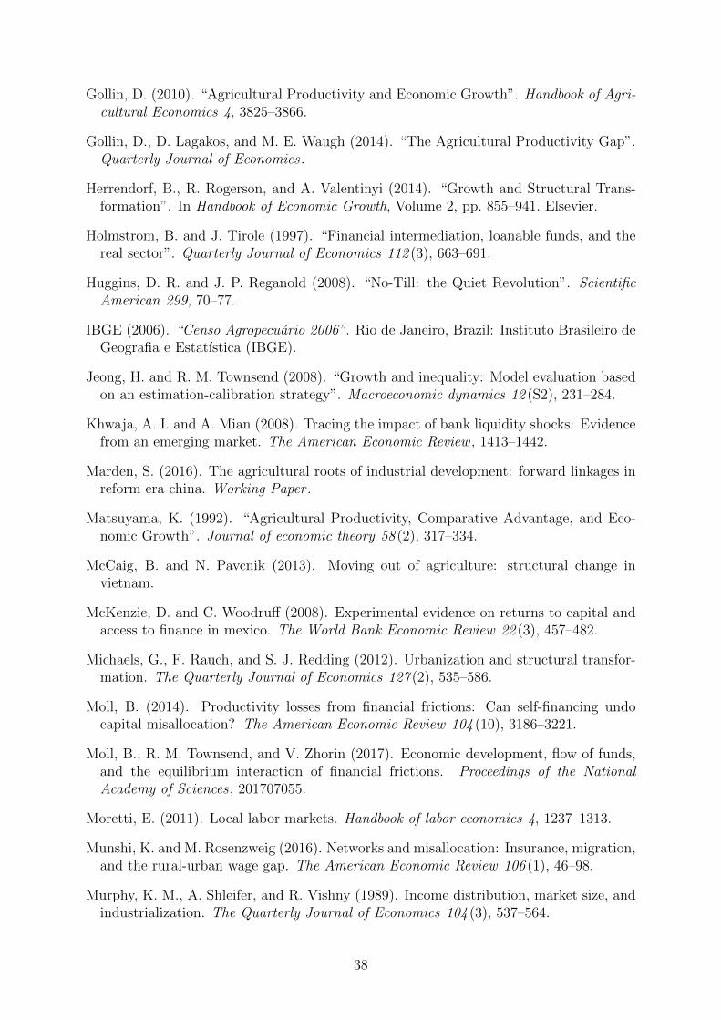
Gollin, D. (2010). “Agricultural Productivity and Economic Growth”. Handbook of Agri-cultural Economics 4, 3825–3866.

Gollin, D., D. Lagakos, and M. E. Waugh (2014). “The Agricultural Productivity Gap”.Quarterly Journal of Economics .

Herrendorf, B., R. Rogerson, and A. Valentinyi (2014). “Growth and Structural Trans-formation”. In Handbook of Economic Growth, Volume 2, pp. 855–941. Elsevier.

Holmstrom, B. and J. Tirole (1997). “Financial intermediation, loanable funds, and thereal sector”. Quarterly Journal of Economics 112 (3), 663–691.

Huggins, D. R. and J. P. Reganold (2008). “No-Till: the Quiet Revolution”. ScientificAmerican 299, 70–77.

IBGE (2006). “Censo Agropecuario 2006”. Rio de Janeiro, Brazil: Instituto Brasileiro deGeografia e Estatıstica (IBGE).

Jeong, H. and R. M. Townsend (2008). “Growth and inequality: Model evaluation basedon an estimation-calibration strategy”. Macroeconomic dynamics 12 (S2), 231–284.

Khwaja, A. I. and A. Mian (2008). Tracing the impact of bank liquidity shocks: Evidencefrom an emerging market. The American Economic Review , 1413–1442.

Marden, S. (2016). The agricultural roots of industrial development: forward linkages inreform era china. Working Paper .

Matsuyama, K. (1992). “Agricultural Productivity, Comparative Advantage, and Eco-nomic Growth”. Journal of economic theory 58 (2), 317–334.

McCaig, B. and N. Pavcnik (2013). Moving out of agriculture: structural change invietnam.

McKenzie, D. and C. Woodruff (2008). Experimental evidence on returns to capital andaccess to finance in mexico. The World Bank Economic Review 22 (3), 457–482.

Michaels, G., F. Rauch, and S. J. Redding (2012). Urbanization and structural transfor-mation. The Quarterly Journal of Economics 127 (2), 535–586.

Moll, B. (2014). Productivity losses from financial frictions: Can self-financing undocapital misallocation? The American Economic Review 104 (10), 3186–3221.

Moll, B., R. M. Townsend, and V. Zhorin (2017). Economic development, flow of funds,and the equilibrium interaction of financial frictions. Proceedings of the NationalAcademy of Sciences , 201707055.

Moretti, E. (2011). Local labor markets. Handbook of labor economics 4, 1237–1313.

Munshi, K. and M. Rosenzweig (2016). Networks and misallocation: Insurance, migration,and the rural-urban wage gap. The American Economic Review 106 (1), 46–98.

Murphy, K. M., A. Shleifer, and R. Vishny (1989). Income distribution, market size, andindustrialization. The Quarterly Journal of Economics 104 (3), 537–564.

38

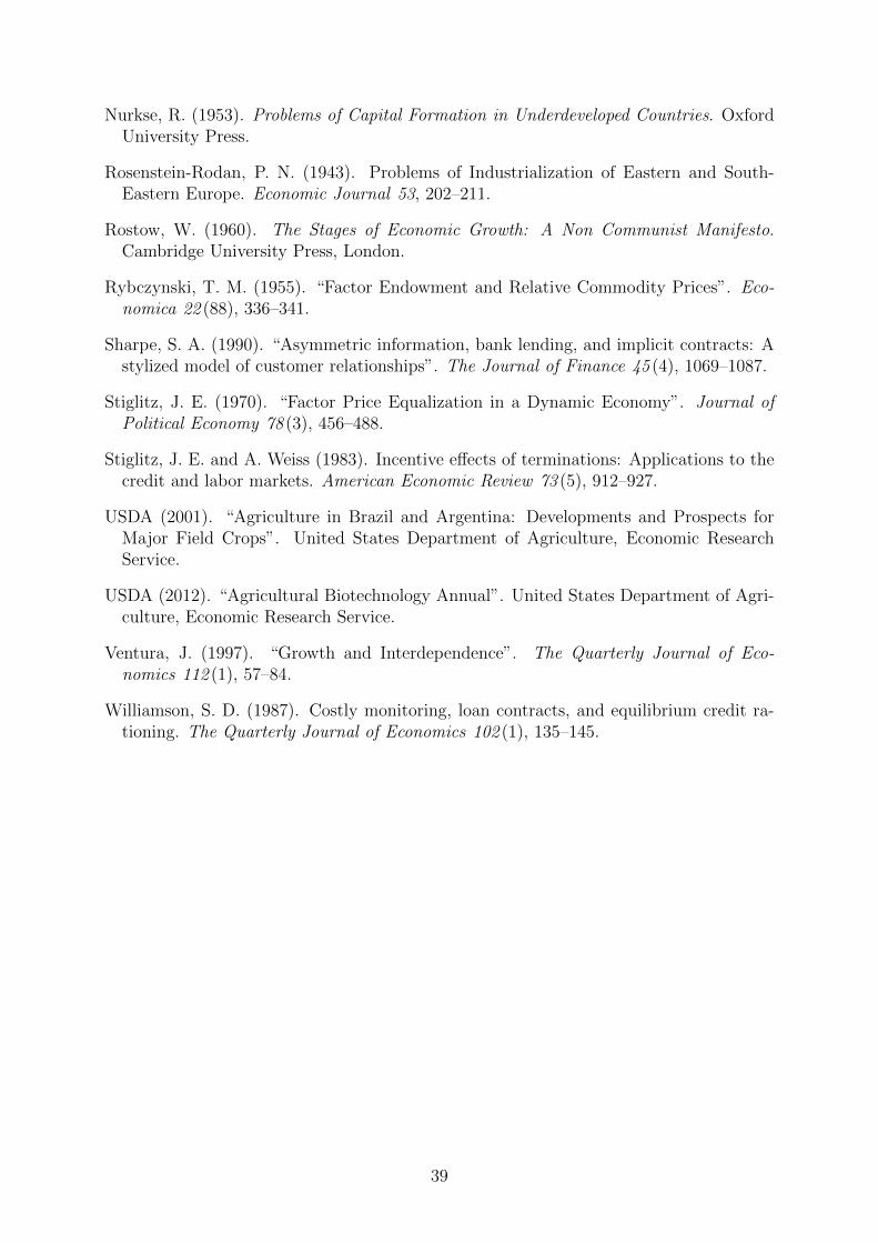
Nurkse, R. (1953). Problems of Capital Formation in Underdeveloped Countries. OxfordUniversity Press.

Rosenstein-Rodan, P. N. (1943). Problems of Industrialization of Eastern and South-Eastern Europe. Economic Journal 53, 202–211.

Rostow, W. (1960). The Stages of Economic Growth: A Non Communist Manifesto.Cambridge University Press, London.

Rybczynski, T. M. (1955). “Factor Endowment and Relative Commodity Prices”. Eco-nomica 22 (88), 336–341.

Sharpe, S. A. (1990). “Asymmetric information, bank lending, and implicit contracts: Astylized model of customer relationships”. The Journal of Finance 45 (4), 1069–1087.

Stiglitz, J. E. (1970). “Factor Price Equalization in a Dynamic Economy”. Journal ofPolitical Economy 78 (3), 456–488.

Stiglitz, J. E. and A. Weiss (1983). Incentive effects of terminations: Applications to thecredit and labor markets. American Economic Review 73 (5), 912–927.

USDA (2001). “Agriculture in Brazil and Argentina: Developments and Prospects forMajor Field Crops”. United States Department of Agriculture, Economic ResearchService.

USDA (2012). “Agricultural Biotechnology Annual”. United States Department of Agri-culture, Economic Research Service.

Ventura, J. (1997). “Growth and Interdependence”. The Quarterly Journal of Eco-nomics 112 (1), 57–84.

Williamson, S. D. (1987). Costly monitoring, loan contracts, and equilibrium credit ra-tioning. The Quarterly Journal of Economics 102 (1), 135–145.

39

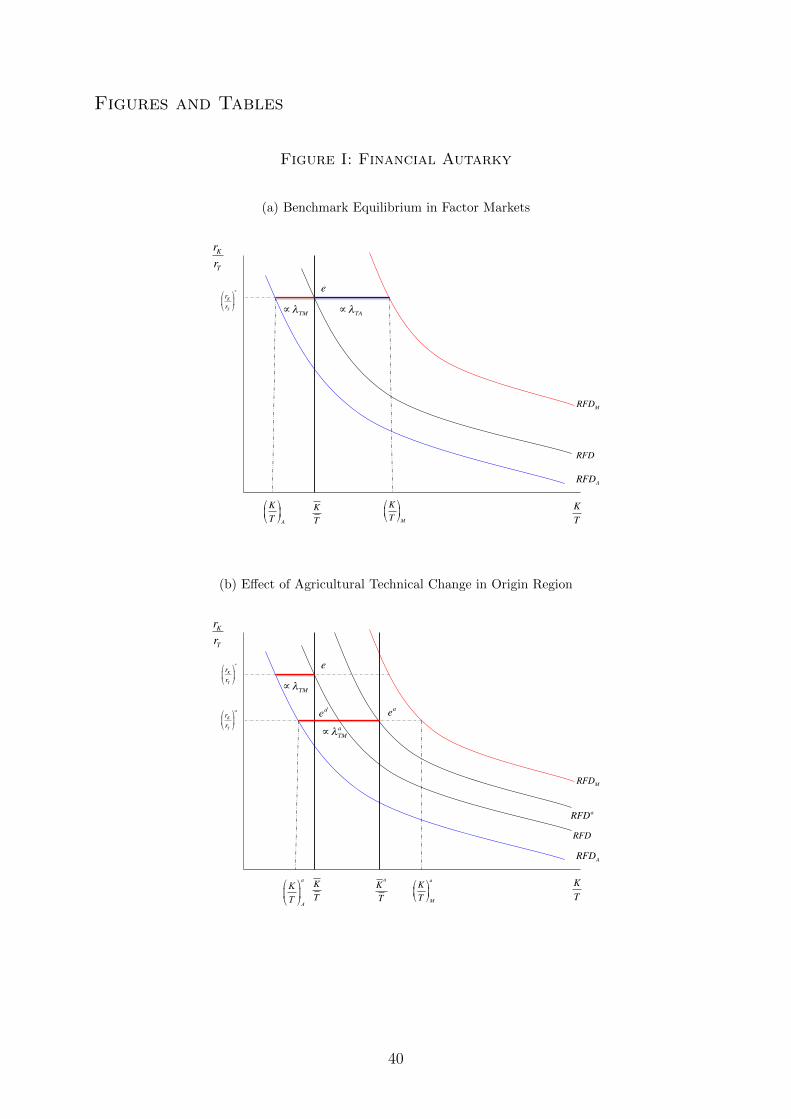
Figures and Tables

Figure I: Financial Autarky

(a) Benchmark Equilibrium in Factor Markets

rKrT

KT

RFDM

RFDA

KT!

"#

$

%&A

KT

KT!

"#

$

%&M

e

RFD

∝λTM

rKrT

!

"#

$

%&

*

∝λTA

(b) Effect of Agricultural Technical Change in Origin Region

rKrT

KT

RFDM

RFDA

KT⎛

⎝⎜

⎞

⎠⎟A

a KT

rKrT

!

"#

$

%&

*

KT!

"#

$

%&M

a

e

rKrT

!

"#

$

%&

a ed ea

RFDa

RFD

Ka

T

∝λTM

∝λ aTM

40

Figure II: Financial Integration: Origin Region

rK

rT

KT

RFDM

RFDA

KT

rK

rT

* e

rK

rT

a

r*K

rTi

K d

T

ei

CapitalOutflow

K s

T

Figure III: Financial Integration: Destination Region

rK

rT

KT

RFDM

RFDA

KT

A

KT

rK

rT

*

rK

rT

i

KT

M

e

RFD

iTM

KSi

T

ei

CapitalInflow

41

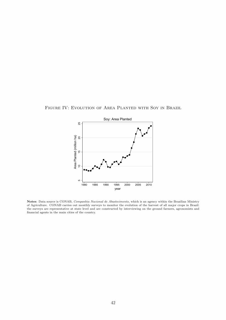
Figure IV: Evolution of Area Planted with Soy in Brazil

510

1520

25A

rea

Pla

nted

(mill

ion

ha)

1980 1985 1990 1995 2000 2005 2010year

Soy: Area Planted

Notes: Data source is CONAB, Companhia Nacional de Abastecimento, which is an agency within the Brazilian Ministryof Agriculture. CONAB carries out monthly surveys to monitor the evolution of the harvest of all major crops in Brazil:the surveys are representative at state level and are constructed by interviewing on the ground farmers, agronomists andfinancial agents in the main cities of the country.

42

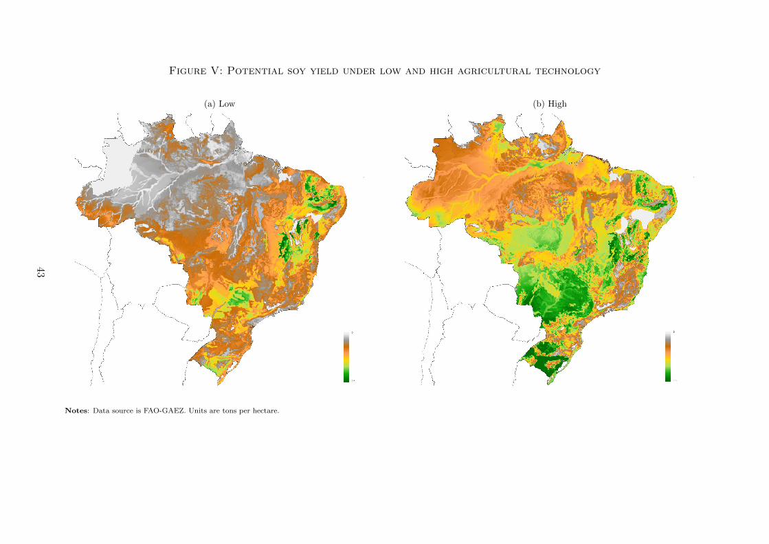
Figure V: Potential soy yield under low and high agricultural technology

(a) Low (b) High

Notes: Data source is FAO-GAEZ. Units are tons per hectare.

43

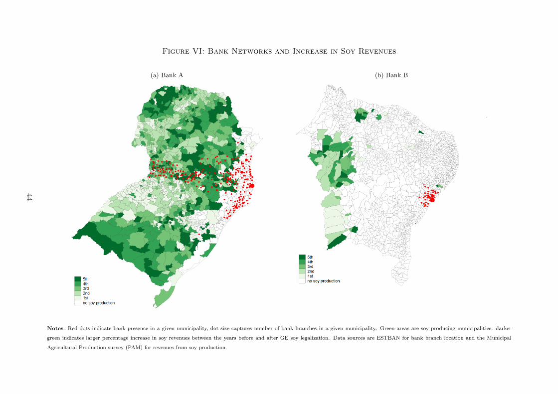
Figure VI: Bank Networks and Increase in Soy Revenues

(a) Bank A (b) Bank B

Notes: Red dots indicate bank presence in a given municipality, dot size captures number of bank branches in a given municipality. Green areas are soy producing municipalities: darker

green indicates larger percentage increase in soy revenues between the years before and after GE soy legalization. Data sources are ESTBAN for bank branch location and the Municipal

Agricultural Production survey (PAM) for revenues from soy production.

44

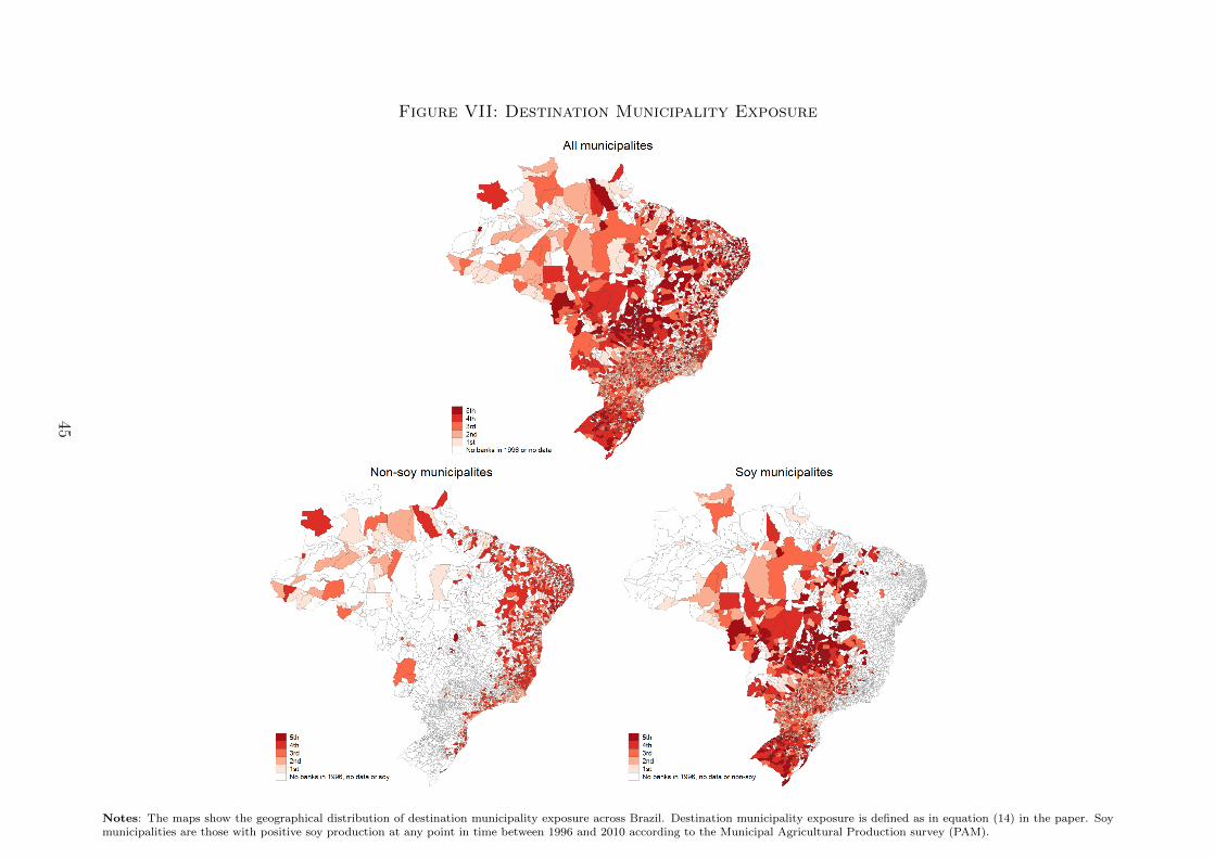
Figure VII: Destination Municipality Exposure

Notes: The maps show the geographical distribution of destination municipality exposure across Brazil. Destination municipality exposure is defined as in equation (14) in the paper. Soymunicipalities are those with positive soy production at any point in time between 1996 and 2010 according to the Municipal Agricultural Production survey (PAM).

45

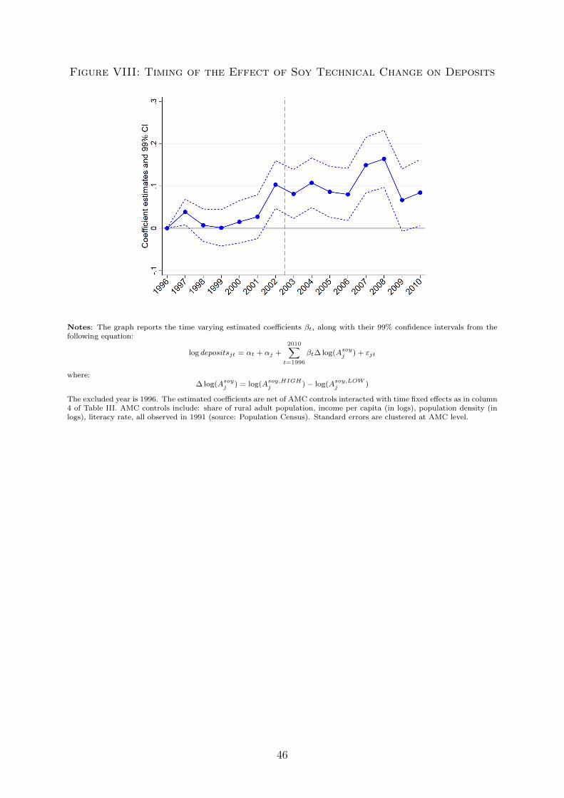
Figure VIII: Timing of the Effect of Soy Technical Change on Deposits

Notes: The graph reports the time varying estimated coefficients βt, along with their 99% confidence intervals from thefollowing equation:

log depositsjt = αt + αj +2010∑

t=1996

βt∆ log(Asoyj ) + εjt

where:∆ log(Asoy

j ) = log(Asoy,HIGHj )− log(Asoy,LOW

j )

The excluded year is 1996. The estimated coefficients are net of AMC controls interacted with time fixed effects as in column4 of Table III. AMC controls include: share of rural adult population, income per capita (in logs), population density (inlogs), literacy rate, all observed in 1991 (source: Population Census). Standard errors are clustered at AMC level.

46

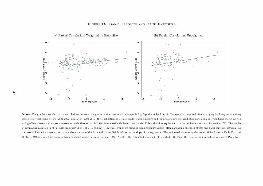
Figure IX: Bank Deposits and Bank Exposure

(a) Partial Correlation, Weighted by Bank Size

-6-4

-20

24

Dep

osit

Gro

wth

(log

)

-.4 -.2 0 .2 .4Bank Exposure

(b) Partial Correlation, Unweighted

-6-4

-20

24

Dep

osit

Gro

wth

(log

)

-.4 -.2 0 .2 .4Bank Exposure

Notes: The graphs show the partial correlations between changes in bank exposure and changes in log deposits at bank level. Changes are computed after averaging bank exposure and log

deposits for each bank before (2001-2002) and after (2003-2010) the legalization of GE soy seeds. Bank exposure and log deposits are averaged after partialling out year fixed effects, as well

as log of bank assets and deposit-to-asset ratio (both observed in 1996) interacted with linear time trends. This is therefore equivalent to a first difference version of equation (??). The results

of estimating equation (??) in levels are reported in Table V, column 4. In these graphs we focus on bank exposure values (after partialling out fixed effects and bank controls) between -0.5

and +0.5. This is for a more transparent visualization of the data and has negligible effects on the slope of the regression. The estimated slope using the same 121 banks as in Table V is 1.81

(t-stat = 2.25), while if we focus on bank exposure values between -0.5 and +0.5 (N=114), the estimated slope is 2.12 (t-stat=2.44). Panel (b) reports the unweighted version of Panel (a).

47

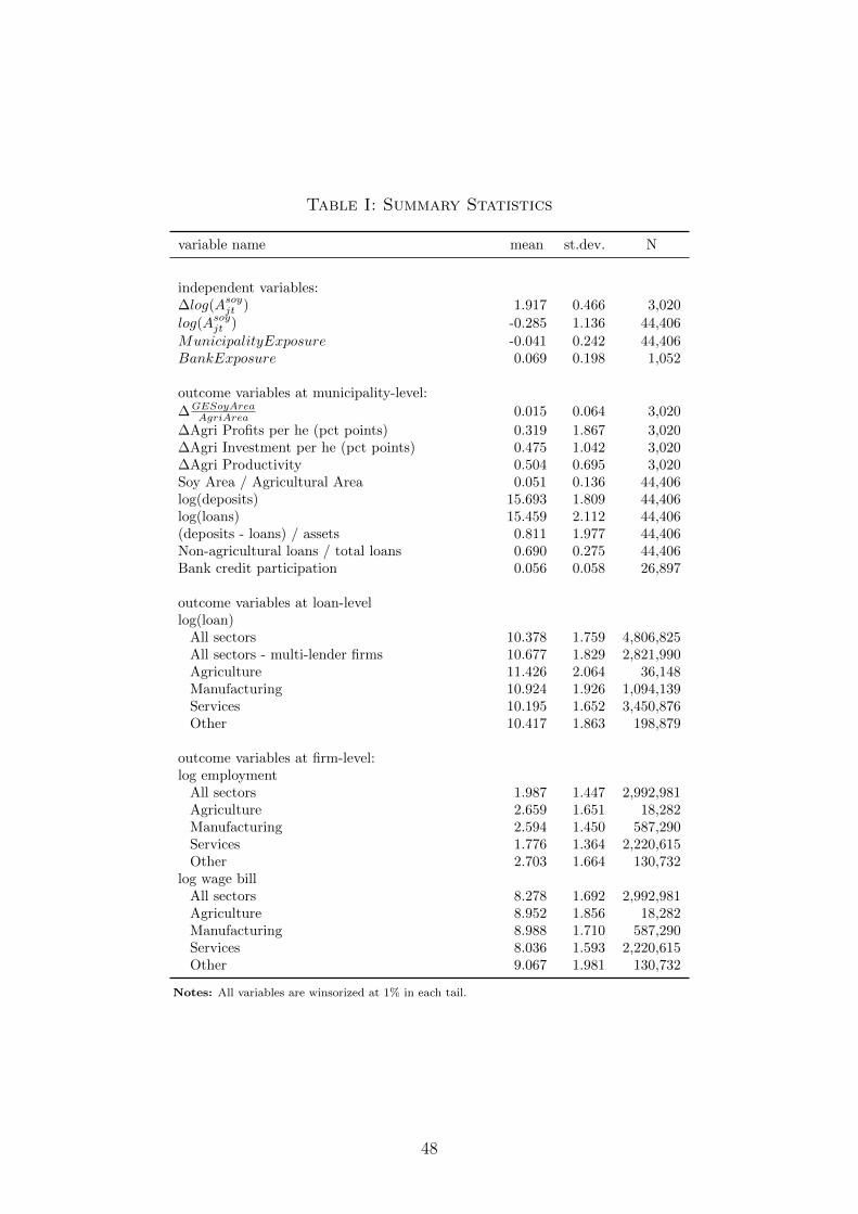
Table I: Summary Statistics

variable name mean st.dev. N

independent variables:∆log(Asoy

jt ) 1.917 0.466 3,020

log(Asoyjt ) -0.285 1.136 44,406

MunicipalityExposure -0.041 0.242 44,406BankExposure 0.069 0.198 1,052

outcome variables at municipality-level: ahksadhf

∆GESoyAreaAgriArea 0.015 0.064 3,020

∆Agri Profits per he (pct points) 0.319 1.867 3,020∆Agri Investment per he (pct points) 0.475 1.042 3,020∆Agri Productivity 0.504 0.695 3,020Soy Area / Agricultural Area 0.051 0.136 44,406log(deposits) 15.693 1.809 44,406log(loans) 15.459 2.112 44,406(deposits - loans) / assets 0.811 1.977 44,406Non-agricultural loans / total loans 0.690 0.275 44,406Bank credit participation 0.056 0.058 26,897

outcome variables at loan-levellog(loan)

All sectors 10.378 1.759 4,806,825All sectors - multi-lender firms 10.677 1.829 2,821,990Agriculture 11.426 2.064 36,148Manufacturing 10.924 1.926 1,094,139Services 10.195 1.652 3,450,876Other 10.417 1.863 198,879

outcome variables at firm-level:log employment

All sectors 1.987 1.447 2,992,981Agriculture 2.659 1.651 18,282Manufacturing 2.594 1.450 587,290Services 1.776 1.364 2,220,615Other 2.703 1.664 130,732

log wage billAll sectors 8.278 1.692 2,992,981Agriculture 8.952 1.856 18,282Manufacturing 8.988 1.710 587,290Services 8.036 1.593 2,220,615Other 9.067 1.981 130,732

Notes: All variables are winsorized at 1% in each tail.

48

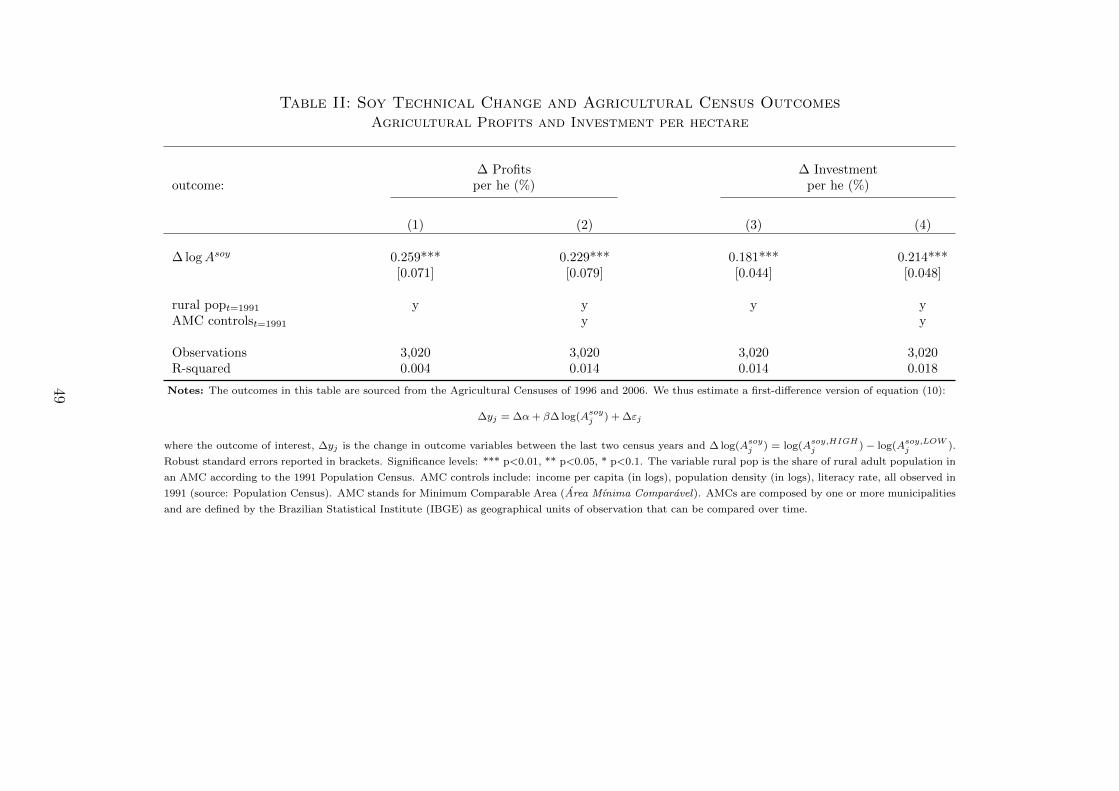
Table II: Soy Technical Change and Agricultural Census OutcomesAgricultural Profits and Investment per hectare

∆ Profits ∆ Investmentoutcome: per he (%) per he (%)

(1) (2) (3) (4)

∆ logAsoy 0.259*** 0.229*** 0.181*** 0.214***[0.071] [0.079] [0.044] [0.048]

rural popt=1991 y y y yAMC controlst=1991 y y

Observations 3,020 3,020 3,020 3,020R-squared 0.004 0.014 0.014 0.018

Notes: The outcomes in this table are sourced from the Agricultural Censuses of 1996 and 2006. We thus estimate a first-difference version of equation (10):

∆yj = ∆α+ β∆ log(Asoyj ) + ∆εj

where the outcome of interest, ∆yj is the change in outcome variables between the last two census years and ∆ log(Asoyj ) = log(Asoy,HIGH

j ) − log(Asoy,LOWj ).

Robust standard errors reported in brackets. Significance levels: *** p<0.01, ** p<0.05, * p<0.1. The variable rural pop is the share of rural adult population in

an AMC according to the 1991 Population Census. AMC controls include: income per capita (in logs), population density (in logs), literacy rate, all observed in

1991 (source: Population Census). AMC stands for Minimum Comparable Area (Area Mınima Comparavel). AMCs are composed by one or more municipalities

and are defined by the Brazilian Statistical Institute (IBGE) as geographical units of observation that can be compared over time.

49

Table III: Local Effects of Soy Technical ChangeSoy Area Share, Deposits, Loans and Capital Export

outcome: log(deposits) log(loans) deposits−loansassets

(1) (2) (3) (4) (5) (6)

logAsoy 0.060*** 0.070*** -0.077*** -0.061** 0.305*** 0.297***[0.016] [0.016] [0.029] [0.029] [0.062] [0.065]

AMC fe y y y y y yyear fe y y y y y yrural popt=1991 × year fe y y y y y yAMC controlst=1991 × year fe y y y

Observations 44,406 44,406 44,406 44,406 44,406 44,406R-squared 0.975 0.976 0.951 0.951 0.711 0.713N clusters 3145 3145 3145 3145 3145 3145

Notes: Standard errors clustered at AMC level are reported in brackets. Significance levels: *** p<0.01, ** p<0.05, * p<0.1. The variable rural pop is the share

of rural adult population in an AMC according to the 1991 Population Census. AMC controls include: income per capita (in logs), population density (in logs),

literacy rate, all observed in 1991 (source: Population Census). AMC stands for Minimum Comparable Area (Area Mınima Comparavel). AMCs are composed

by one or more municipalities and are defined by the Brazilian Statistical Institute (IBGE) as geographical units of observation that can be compared over time.

50

Table IV: Capital Reallocation Across MunicipalitiesLending and Non-Agricultural Lending Share

outcome: log(loans) non-agricultural loanstotal loans

sample: all soy non-soy all soy non-soyregion region region region

(1) (2) (3) (4) (5) (6)

MunicipalityExposuredt 0.283*** 0.054 0.580*** 0.090*** 0.046* 0.139***[0.090] [0.124] [0.131] [0.016] [0.024] [0.023]

AMC fe y y y y y yyear fe y y y y y yrural popt=1991 × year fe y y y y y yAMC controlst=1991 × year fe y y y y y y

Observations 44,406 22,550 21,856 44,406 22,550 21,856R-squared 0.952 0.949 0.953 0.843 0.846 0.779N clusters 3145 1565 1580 3145 1565 1580

Notes: Standard errors clustered at AMC level are reported in brackets. Significance levels: *** p<0.01, ** p<0.05, * p<0.1.The variable rural pop is the share

of rural adult population in an AMC according to the 1991 Population Census. AMC controls include: income per capita (in logs), population density (in logs),

literacy rate, all observed in 1991 (source: Population Census). AMC stands for Minimum Comparable Area (Area Mınima Comparavel). AMCs are composed

by one or more municipalities and are defined by the Brazilian Statistical Institute (IBGE) as geographical units of observation that can be compared over time.

51

Table V: Bank Deposits and Bank Exposure

outcome: log deposits

(1) (2) (3) (4)

BankExposurebt 1.427** 1.664*** 1.580** 1.750**[0.587] [0.562] [0.761] [0.688]

Log Assetsb,t=0 × t -0.012 -0.010[0.010] [0.012]

Deposits/Assetsb,t=0 × t -0.085 -0.068[0.140] [0.151]

bank fe y y y yyear fe y y y y

Observations 1,052 1,052 1,052 1,052R-squared 0.913 0.913 0.913 0.913N clusters 121 121 121 121

Notes: Standard errors clustered at bank level are reported in brackets. Significance levels: *** p<0.01, ** p<0.05, *

p<0.1. Regressions are weighted by total bank assets in 1996. Bank controls are observed in 1996 (source: ESTBAN) and

interacted with linear time trends.

52

Table VI: The Effect of Bank Exposure on LoansLoan Value

outcome: log loan

multi-lender(1) (2) (3) (4)

BankExposurebt 0.257 0.290 0.280 0.228[0.124]** [0.108]*** [0.108]** [0.095]**

fixed effects:firm y y y yyear y y y ybank y y y yAMC × year y y ySector × year y y yfirm × year y

Observations 4,806,825 4,806,825 2,821,990 2,821,990R-squared 0.549 0.554 0.536 0.664N clusters 115 115 115 115

Notes: Standard errors clustered at bank level reported in brackets. Significance levels: *** p<0.01, ** p<0.05, *

p<0.1. AMC stands for Minimum Comparable Area (Area Mınima Comparavel). AMCs are composed by one or more

municipalities and are defined by the Brazilian Statistical Institute (IBGE) as geographical units of observation that can be

compared over time. Sector dummies correspond to the 87 2-digit sectors according to the Brazilian CNAE 2.0 classification.

53

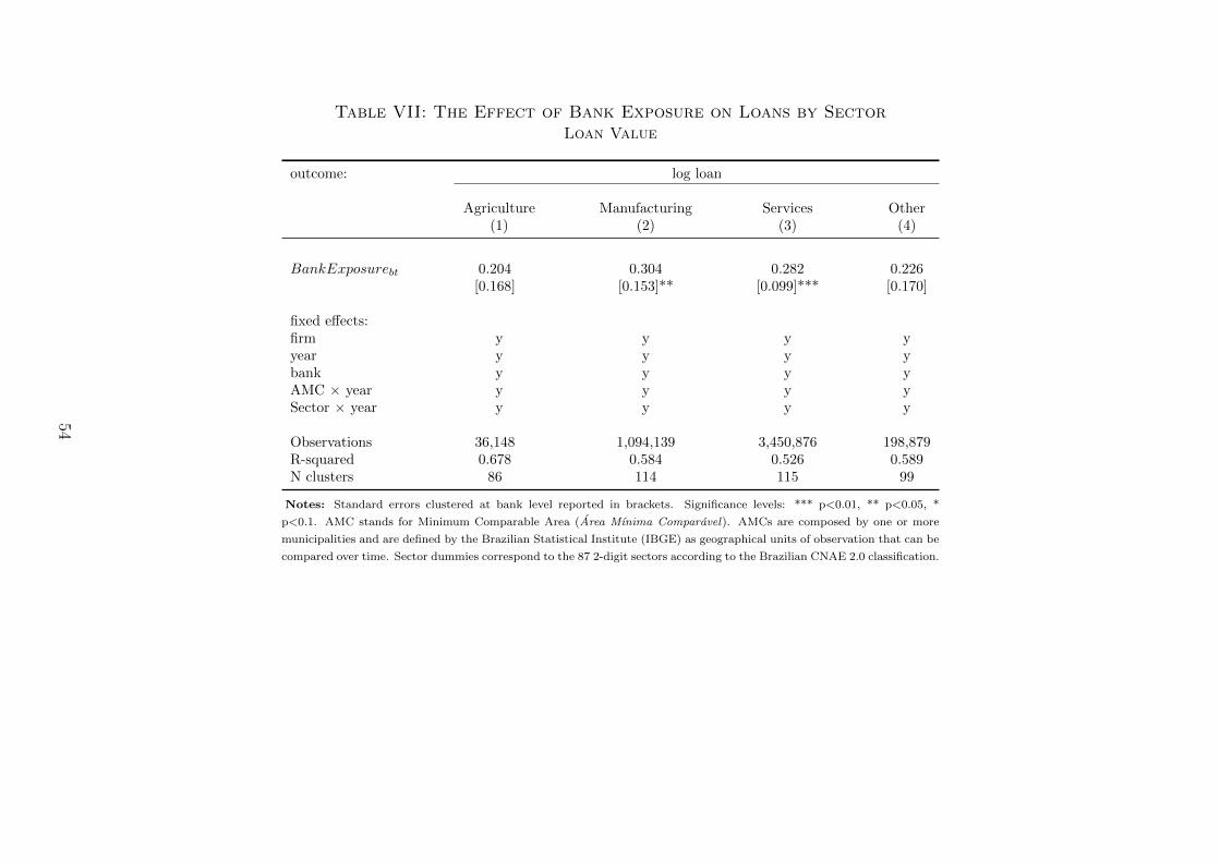
Table VII: The Effect of Bank Exposure on Loans by SectorLoan Value

outcome: log loan

Agriculture Manufacturing Services Other(1) (2) (3) (4)

BankExposurebt 0.204 0.304 0.282 0.226[0.168] [0.153]** [0.099]*** [0.170]

fixed effects:firm y y y yyear y y y ybank y y y yAMC × year y y y ySector × year y y y y

Observations 36,148 1,094,139 3,450,876 198,879R-squared 0.678 0.584 0.526 0.589N clusters 86 114 115 99

Notes: Standard errors clustered at bank level reported in brackets. Significance levels: *** p<0.01, ** p<0.05, *

p<0.1. AMC stands for Minimum Comparable Area (Area Mınima Comparavel). AMCs are composed by one or more

municipalities and are defined by the Brazilian Statistical Institute (IBGE) as geographical units of observation that can be

compared over time. Sector dummies correspond to the 87 2-digit sectors according to the Brazilian CNAE 2.0 classification.

54

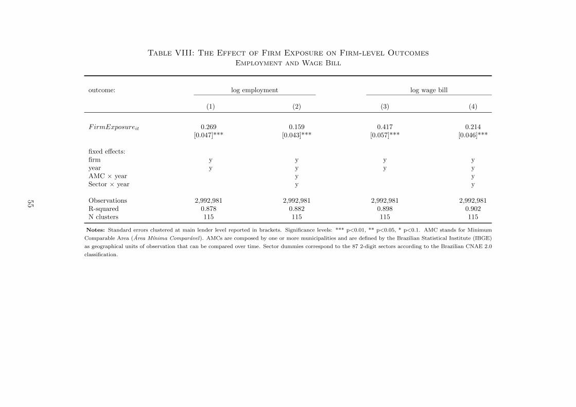
Table VIII: The Effect of Firm Exposure on Firm-level OutcomesEmployment and Wage Bill

outcome: log employment log wage bill

(1) (2) (3) (4)

FirmExposureit 0.269 0.159 0.417 0.214[0.047]*** [0.043]*** [0.057]*** [0.046]***

fixed effects:firm y y y yyear y y y yAMC × year y ySector × year y y

Observations 2,992,981 2,992,981 2,992,981 2,992,981R-squared 0.878 0.882 0.898 0.902N clusters 115 115 115 115

Notes: Standard errors clustered at main lender level reported in brackets. Significance levels: *** p<0.01, ** p<0.05, * p<0.1. AMC stands for Minimum

Comparable Area (Area Mınima Comparavel). AMCs are composed by one or more municipalities and are defined by the Brazilian Statistical Institute (IBGE)

as geographical units of observation that can be compared over time. Sector dummies correspond to the 87 2-digit sectors according to the Brazilian CNAE 2.0

classification.

55

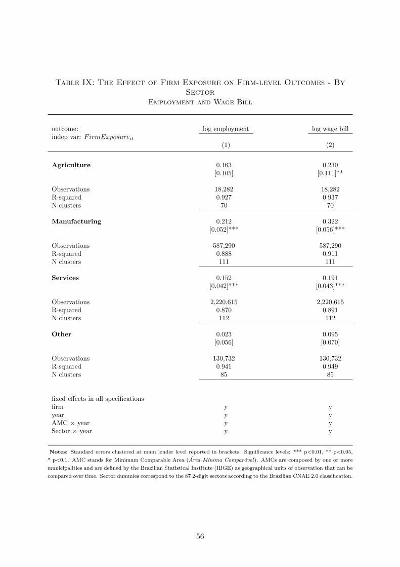
Table IX: The Effect of Firm Exposure on Firm-level Outcomes - BySector

Employment and Wage Bill

outcome: log employment log wage billindep var: FirmExposureit

(1) (2)

Agriculture 0.163 0.230[0.105] [0.111]**

Observations 18,282 18,282R-squared 0.927 0.937N clusters 70 70

Manufacturing 0.212 0.322[0.052]*** [0.056]***

Observations 587,290 587,290R-squared 0.888 0.911N clusters 111 111

Services 0.152 0.191[0.042]*** [0.043]***

Observations 2,220,615 2,220,615R-squared 0.870 0.891N clusters 112 112

Other 0.023 0.095[0.056] [0.070]

Observations 130,732 130,732R-squared 0.941 0.949N clusters 85 85

fixed effects in all specificationsfirm y yyear y yAMC × year y ySector × year y y

Notes: Standard errors clustered at main lender level reported in brackets. Significance levels: *** p<0.01, ** p<0.05,

* p<0.1. AMC stands for Minimum Comparable Area (Area Mınima Comparavel). AMCs are composed by one or more

municipalities and are defined by the Brazilian Statistical Institute (IBGE) as geographical units of observation that can be

compared over time. Sector dummies correspond to the 87 2-digit sectors according to the Brazilian CNAE 2.0 classification.

56

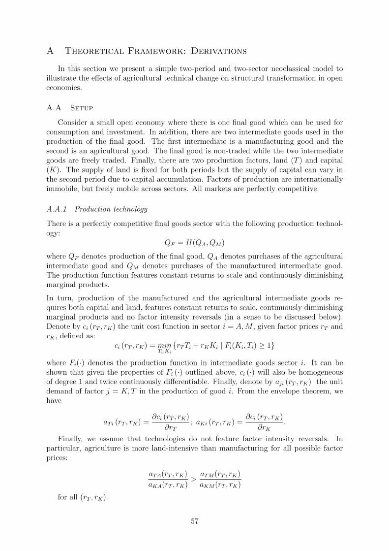
A Theoretical Framework: Derivations

In this section we present a simple two-period and two-sector neoclassical model toillustrate the effects of agricultural technical change on structural transformation in openeconomies.

A.A Setup

Consider a small open economy where there is one final good which can be used forconsumption and investment. In addition, there are two intermediate goods used in theproduction of the final good. The first intermediate is a manufacturing good and thesecond is an agricultural good. The final good is non-traded while the two intermediategoods are freely traded. Finally, there are two production factors, land (T ) and capital(K). The supply of land is fixed for both periods but the supply of capital can vary inthe second period due to capital accumulation. Factors of production are internationallyimmobile, but freely mobile across sectors. All markets are perfectly competitive.

A.A.1 Production technology

There is a perfectly competitive final goods sector with the following production technol-ogy:

QF = H(QA, QM)

where QF denotes production of the final good, QA denotes purchases of the agriculturalintermediate good and QM denotes purchases of the manufactured intermediate good.The production function features constant returns to scale and continuously diminishingmarginal products.

In turn, production of the manufactured and the agricultural intermediate goods re-quires both capital and land, features constant returns to scale, continuously diminishingmarginal products and no factor intensity reversals (in a sense to be discussed below).Denote by ci (rT , rK) the unit cost function in sector i = A,M , given factor prices rT andrK , defined as:

ci (rT , rK) = minTi,Ki

{rTTi + rKKi | Fi(Ki, Ti) ≥ 1}

where Fi(·) denotes the production function in intermediate goods sector i. It can beshown that given the properties of Fi (·) outlined above, ci (·) will also be homogeneousof degree 1 and twice continuously differentiable. Finally, denote by aji (rT , rK) the unitdemand of factor j = K,T in the production of good i. From the envelope theorem, wehave

aT i (rT , rK) =∂ci (rT , rK)

∂rT; aKi (rT , rK) =

∂ci (rT , rK)

∂rK.

Finally, we assume that technologies do not feature factor intensity reversals. Inparticular, agriculture is more land-intensive than manufacturing for all possible factorprices:

aTA(rT , rK)

aKA(rT , rK)>aTM(rT , rK)

aKM(rT , rK)

for all (rT , rK).

57

Agricultural ProductivityWe can consider Hicks-neutral increases in agricultural productivity within this frame-

work by modifying the the production function in agriculture, so that it can be writtenas:

GA(A,KA, TA) = AFA(KA, TA).

In this case, the unit cost function in agriculture is b(A, rT , rK) = 1AcA (rT , rK) and unit

factor demands are:

∂b(A, rT , rK)

∂rT=

1

AaT i (rT , rK) ;

∂b(A, rT , rK)

∂rK=

1

AaKi (rT , rK)

where aTA and aKA can be interpreted as unit factor demands in efficiency units.

A.A.2 Preferences

Individuals in this economy only live for two periods, thus their utility function is:

U(yh1 , y

h2

)= lnyh1 + β lnyh2 (19)

where yht is final good consumption of individual h in period t = 1, 2. Consumption inperiod 1 is the numeraire. There are two assets, land (t) and capital (k). The rental rateof land is rT and its price at the end of period 1 is q. Because the world ends at the endof period 2, land will then have a price of zero. In turn, the rental rate of capital is rK,1and its depreciation rate is δ. Capital is reversible in the sense that it can be turned intoconsumption at the end of period 1, thus its price is equal to one. Then, the individualbudget constraints in periods 1 and 2 are:

yh1 = (rT,1 + q) th1 + [rK,1 + (1− δ)] kh1 − sh

yh2 = rT,2th2 + [rK,2 + (1− δ)] kh2

where sh = qth2 + kh2 are savings.

A.B Equilibrium

In this section we list and solve for the equilibrium conditions of the model. We startby considering the intertemporal equilibrium in asset markets to obtain a solution for thecapital stock in the second period as a function of factor prices. Next, we solve for factorprices in each period using the intra-temporal equilibrium conditions in goods and factormarkets. Note that due to the factor price equalization theorem, factor prices are fullydetermined by technology and international prices (Samuelson, 1949). Thus, factor pricesare independent of savings decisions and local factor supplies.

A.B.1 Intertemporal equilibrium

Portfolio choice Note that because there are two assets, there is an optimal portfoliochoice where individuals compare the return of each asset in terms of second periodconsumption divided by its price in terms of first period consumption. Only when assetreturns are equal, individuals are willing to hold both assets in equilibrium:

58

th2 =

0 if

rT,2

q< rK,2 + (1− δ)[

0, sh]

ifrT,2

q= rK,2 + (1− δ)

sh ifrT,2

q> rK,2 + (1− δ)

Let’s assume the solution is interior. Then, the equilibrium price of land at the end ofthe first period is:

q =rT,2

rK,2 + (1− δ)

Savings If we substitute the price of land in the savings equation, we can write it as:

sh =rT,2

rK,2 + (1− δ)th2 + kh2 .

Then, replace sh in the budget constraint for period 1 by the r.h.s. of the equation justabove to obtain:

yh1 +yh2

rK,2 + (1− δ)= (rT,1 + q) th1 + [rK,1 + (1− δ)] kh1 .

Note that the l.h.s. of the equation above is the present value of lifetime consumptionand the r.h.s. is the present value of wealth. This is because this individual only derivesincome from the two assets t and k, thus their current rents plus prices reflect theirlifetime income streams. Then, optimal consumption in period 1, given Cobb-Douglaspreferences, is a constant fraction of lifetime wealth:

yh1 =1

1 + β

{(rT,1 + q) th1 + [rK,1 + (1− δ)] kh1

}.

In turn, optimal consumption in period 2 can be obtained from the Euler equation:

yh2yh1

= β [rK,2 + (1− δ)] .

Aggregation Land Market Equilibrium implies:∑h

th1 =∑h

th2 = T.

Savings equals Investment yields: ∑h

sh = K2 + qT.

Substitute for sh and q to obtain

K2 =β

1 + β[rK,1 + (1− δ)]K1 +

1

1 + β

[βrT,1 −

rT,2rK,2 + (1− δ)

]T (20)

where Kt denotes the aggregate capital stock in period t and T is the aggregate landendowment.

59

A.B.2 Intratemporal equilibrium

Final good The representative firm in the final goods sector minimizes productioncosts given demand for the final good, which must equal income, thus intermediate gooddemands are

Di = αi(pa, pm) (rKK + rTT ) (21)

where αi(pa, pm) is the share of spending on intermediate good i. Time subscripts areomitted for simplicity. Note that because the final goods sector is competitive, the price ofthe final good must equal unit production costs. Thus, even if the final good is non-traded,its price is given by the international prices of traded intermediates.

Intermediate goods Free trade and perfect competition in the intermediate goodssectors imply that prices equal average (and marginal) production costs in each sector.Denote by Xi > 0 the amount of intermediate good i produced in the country. Perfectcompetition and free trade imply that for each intermediate good i = A,M , we must have

pM ≤ cM (rT , rK) , with strict equality if XM > 0; (22)

pA ≤1

AcA (rT , rK) , with strict equality if XA > 0. (23)

In turn, factor market clearing requires:

aTA (rT , rK) XA + aTM (rT , rK)XM = T (24)

aKA (rT , rK) XA + aKM (rT , rK)XM = K (25)

where XA = XA/A is agricultural output in efficiency units.We consider the case of a small open economy that faces exogenously given goods

prices pA and pM . An intra-temporal equilibrium of a small open economy is a demandvector D = (DA, DM), a production vector X = (XA, XM) and a factor-price vectorω = (rT , rK) such that (3), (4), (5), (6) and (7) are satisfied. Note that provided thatthe small open-economy produces both goods and technologies feature no factor intensityreversals, factor prices will be uniquely pinned down by goods prices, regardless of factorendowments. This is the Factor Price Insensitivity result by Samuelson (1949).60

A.C Comparative statics: the effects of agricultural technical change

In this section we discuss the effects of a permanent increase in agricultural productiv-ity. That is, we compare the equilibrium level of sectoral outputs in two scenarios. Thefirst scenario we study is a benchmark economy which is in a steady state equilibriumwith constant technology, international goods prices and consumption. The second sce-nario we consider is an economy that adopts the new agricultural technology in period 1,but expects an increase in the cost of operating the technology in period 2 due to stricter

60In this case, equations (4) and (5) can be used to solve for factor prices as a function of technologyand goods prices. Setting the zero-profit equations in (4) and (5) to equality, we have a system of twoequations that implicitly define (rT , rK) in terms of (pA,pM ). From Gale and Nikaido (1965), the mappingfrom (rT , rK) to (pA,pM ) is one-to-one provided that the Jacobian of

[cM (rT , rK) , 1

AcA (rT , rK)], which

we call the technology matrix, is nonsingular and aji(rT , rK) > 0. Note that in this case technologies donot feature factor intensity reversals.

60

environmental regulation. The increase in the cost of operating the new technology inperiod 2 is captured in the model by the parameter γ2 which represents the share of agri-cultural output that has to be spent in abatement costs. Thus, if environmental regulationbecomes stricter, γ2 ∈ (0, 1), agricultural technical change generates a larger increase inincome in period one than in period two. In turn, if γ2 = 1 agricultural technical changegenerates a temporary increase in income, as we show below. Instead, if γ2 = 0, theincome increase is permanent.61

A.C.1 Factor Prices

First, we need to assess how agricultural technical change affects factor prices. Forthis purpose, we use the zero-profit conditions (4) and (5), which permit to solve for factorprice changes as a function of goods prices and agricultural technology. Log-differentiatingthem we obtain that changes in goods prices are a weighted average of changes in factorprices:

pA + A = θTArT + (1− θTA)rK

pM = θTM rT + (1− θTM)rK

where θT i = rTaT i/ci is the land share in sector i and hats denote percent changes. Weomit time subscripts for convenience. Next, we can use Cramer’s rule to solve for thechanges in factor prices taking into account that the goods prices are the same in botheconomies (pM = 0 and pA = 0). Thus, in period 1, when only technology changes thechange in factor prices with respect to the steady state economy is:[

ˆrT,1ˆrK,1

]=

[(1−θTM )AθTA−θTM

−θTM AθTA−θTM

]. (26)

In period 2, both technology and environmental regulation change, then the change infactor prices with respect to the steady state economy is[

ˆrT,2ˆrK,2

]=

[(1−θTM )A(1−γ2)

θTA−θTM

−θTM A(1−γ2)θTA−θTM

]. (27)

Then, agricultural technical change increases the return to land and reduces the returnto capital because agriculture is land-intensive (θTA > θTM). This result is similar to theStolper-Samuelson theorem because agricultural productivity growth rises the profitabilityof agricultural production in the same way as increases in agricultural prices. Note thatwhen γ2 > 0, agricultural technical change increases land rents in period 1 more than inperiod 2 when abatement costs increase.

61An alternative scenario in which technology adoption would generate a temporary increase in incomewould be one where the economy is an early adopter of a new agricultural technology in the sense thatit adopts in period 1, while other countries adopt in period 2. When the technology is adopted by othercountries, the international price of the agricultural good falls. We can then parametrize the internationaltechnology adoption rate (γ2) in such a way that if all countries in the world adopt the technology theinternational price of agricultural goods falls in proportion to the productivity improvement. This impliesthat agricultural technical change generates a temporary increase in income for the early adopter. Instead,if no other country adopts in period 2 the income increase is permanent.

61

A.C.2 Agricultural and manufacturing output

Next, we analyze the effect of agricultural technical change on agricultural and man-ufacturing output by using the factor market clearing conditions (6) and (7). Log-differentiating we obtain:

(1− λKM) ˆXA + λKMXM + (1− λKM) ˆaKA + λKM ˆaKM = K (28)

(1− λTM) ˆXA + λTMXM + (1− λTM) ˆaTA + λTM ˆaTM = T (29)

whereλiM = aiMXM/K is the share of factor i employed in sector M . We can show thatλKM > λTM if and only if sector M is capital intensive relative to A. We solve for changesin factor intensities by using the cost minimization conditions, which imply:

θKA ˆaKA + θTA ˆaTA = 0 (30)

θKM ˆaKM + θTM ˆaTM = 0. (31)

Elasticities of substitution across factors in each sector can be defined as:

σA = − ˆaKA − ˆaTArK − rT

(32)

σM = − ˆaKM − ˆaTMrK − rT

(33)

Using equations (12) to (15) we can find the following solutions for aji:

ˆaKi = −θT iσi (rK − rT ) ; i = A,M.

aT i = θKiσi (rK − rT ) . i = A,M.

These solutions for aji can be substituted in equations (10) and (11) to obtain:

(1− λKM) ˆXA + λKMXM = K + δK (rK − rT ) (34)

(1− λTM) ˆXA + λTMXM = T − δT (rK − rT ) (35)

where

δK = λKMθTMσM + λKAθTAσA

δT = λTMθKMσM + λTAθKAσA.

Next, to obtain relative outputs, subtract (17) from (16) to get:

XM − ˆXA =1

λKM − λTM

(K − T

)+

(δK + δT )

λKM − λTM(rK − rT ) . (36)

Finally, let’s substitute changes in factor prices by changes in commodity prices or tech-nology, using the zero profit condition to obtain:

62

XM − ˆXA =1

λKM − λTM

(K − T

)+ σs

(pM − pA − A

), (37)

where

σs =(δK + δT )

λKM − λTM1

θKM − θKA;

σs represents the supply elasticity of substitution between commodities, that is, the per-cent change in the relative supply of manufacturing goods for a given change in the relativeprice of manufacturing.

The first term in the r.h.s. of equation (19) represents the capital supply effect ofagricultural technical change while the second term represents the capital demand effect.The first effect takes place when agricultural technical change increases savings and the

supply of capital. In this case K > 0 = T and λKM > λTM , then XM > K > 0 > ˆXA.This is an application of the Rybczinsky theorem which states that an increase in thesupply of capital increases the supply of manufacturing, the capital-intensive sector. Thisis because, given factor prices, the only way to equilibrate factor markets is to assign thenew capital (and some additional capital and land) to the capital-intensive sector. Thesecond term represents the capital demand effect, which takes place because agriculturaltechnical change increases the profitability of the agricultural sector and thus generatesa reallocation of factors towards it, increasing the relative supply of agricultural goods.Because the capital supply and demand effects work in opposite directions, to understandthe effects of agricultural productivity growth on manufacturing output we need to solvefor effect of technical change on the supply of capital, which we do next.

A.C.3 The Supply of Capital

Steady State In this section, we obtain the effects of agricultural technical change onthe supply of capital. For this purpose, we compare the benchmark economy which ison a steady state with constant consumption to the economy where there is agriculturaltechnical change. Let’s start by describing the steady state equilibrium. If this equilibriumfeatures constant consumption, then the Euler equation implies that initial steady stateparameter values should be such that β [rK + (1− δ)] = 1. In this case, the capitalaccumulation condition (2) can be simplified to reflect this parameter restriction andconstant factor prices, as follows:

K2 =1

1 + βK1.

Note that in this case, the capital stock falls over time because the world ends at the endof period 2. Thus, consumers eat part of the capital stock in each period. Capital behavesas an endowment, part of which is consumed each period to smooth consumption.

Effects of agricultural technical change To obtain the effects of technical changeon the supply of capital we start by differentiating the capital accumulation condition (2),under the assumption that depreciation is equal to one:

dK2 =β

1 + β

(drK1

rK1

rK1K1 +drT,1rT,1

rT,1T

)− 1

1 + β

{drT,2rT,2

− drK,2rK,2

}rT,2rK,2

T.

63

Next, from equations (8) and (9) we can obtain that the time path of factor price changessatisfies: ˆrj,2 = ˆrj,1(1 − γ2) for j = T,K and substitute in the equation above, whichyields:

dK2 =β

1 + β

(drK1

rK1

rK1K1 +drT,1rT,1

rT,1T

)− β

1 + β(1− γ2)

{drT,1rT,1

− drK1

rK1

}rT,2βrK,2

T.

Next, we evaluate at the steady state where: βrK,2 = βrK,1 = 1 and rT,1 = rT,2, thusθTM,1 = θTM,2 = θTM to obtain:

dK2 =β

1 + β

drT,1rT,1

rT,1Tγ2 +β

1 + β

drK1

rK1

(rK1K1 + (1− γ2)rT,1T ) .

Note that if γ2 > 0, the first term is positive. In this case, agricultural technical changeincreases land rents in period 1 more than in period 2. Thus, the increase in period1 income is partly temporary, which increases savings and the capital stock in period2, relative to the steady state. The second term, instead, is negative as it representsthe effect of the reduction in the rental price of capital due to agricultural technicalchange. This reduces first period income and the discount rate, which generates anincrease in the present value of second period land income. Thus, the reduction in therental rate of capital reallocates income towards the second period, which reduces savingsand the capital stock. To understand which effect dominates, we need to substitute forthe factor price changes obtained in equation (8) and denote the land income share asαT = rTT/(rKK + rTT ) to obtain, after some algebra:

dK2

K2

=A

θTA − θTM1

1− αT,1{αT,1γ2 − θTM} . (38)

Then, K2 > 0 if αTγ2 > θTM .When the productivity shock is purely transitory (γ2 = 1),the condition for the capital supply to increase is that the land share in the aggregateeconomy is larger than the land share in manufacturing. This condition always holdsif agriculture is land-intensive. To see this, note that the land share can be written asαT = θTAφA + θTM (1− φA) where φA is the income share of the agricultural sector.62

The interpretation of this condition is that the positive temporary income shock dueto land rents increasing is larger the higher is the land share of aggregate income, whilethe negative temporary income shock due to the reduction in the return to capital isproportional to the land share in manufacturing. If the shock is to some extent temporary,γ2ε(0, 1)), the condition is more likely to hold if the difference in land-intensity betweensectors is high, the income share of agriculture is high, and the shock is not too temporary.Finally, if the shock is permanent (γ2 = 0) the condition never holds.

62This is because

αT =rTT

rKK + rTT=

rTaTApAXA

cA [rKK + rTT ]+

rT,1aTMpMXM

cM [rKK + rTT ]= θTA

pAXA

[rKK + rTT ]+ θTM

pMXM

[rKK + rTT ]

= θTArKKA + rTTA[rKK + rTT ]

+ θTMrKKM + rTTM[rKK + rTT ]

= θTAφA + θTM (1− φA) .

64

A.C.4 Capital supply and capital demand effects

The final step is to substitute the solution for K2 given by (20) into equation (19) toevaluate the relative strenghts of the capital supply vs capital demand effects, to obtain:

XM − ˆXA =1

λKM − λTM

A

θKM − θKA

{1

1− αT,1{αT,1γ2 − θTM} − (δK + δT ) (1− γ2)

}(39)

Because manufacturing is capital intensive λKM > λTM and θKM > θKA. Thus, manufac-turing output expands if the term in brackets is positive:

1

1− αT,1{αT,1γ2 − θTM} − (δK + δT ) (1− γ2) > 0

The first term in the expression above reflects the capital supply effect: an increase inthe supply of capital increases manufacturing output (Rybczinsky effect). This effect isstrongest the larger the aggregate land share (αT ) relative to the land share in manufac-turing (θTM). Because the difference in land share between manufacturing and agricultureis high and agriculture is large sector in Brazil, we expect this term to be large in ourcontext. The second term is the capital demand effect: as agriculture becomes moreproductive land rents grow and the rental rate of capital falls. As a result, both sec-tors use less land and more capital. Thus, the capital intensive sector must contract.The strength of this effect is governed by δK and δT . The first is the aggregate percentincrease in capital input demand associated with a one percent reduction in rK/rT result-ing from adjustment to more capital-intensive techniques in both sectors, and the secondis the aggregate percent reduction in land input demand associated with a one percentreduction in rK/rT resulting from adjustment to less land-intensive techniques in bothsectors. These terms are larger the larger is the elasticity of substitution across factorsin agricultural and manufacturing production (σM and σA). Because land and capitalplay very different roles both in agricultural and manufacturing production, we expectthese elasticities to be quite low. Thus, the supply effect is likely to dominate the demandeffect. Still, this is an empirical question that we answer in the following section. Finally,note that the income shock is more temporary the closer is γ2 to one. A more temporaryincome shock reinforces the capital supply effect due to stronger savings and reduces thecapital demand effect due to lower profitability of producing agricultural goods in thesecond period.

A.D Capital Flows

We can use the model developed above to think about the consequences of financialintegration across regions. To simplify the exposition, suppose that the country has tworegions, Origin (o) and Destination (d), which are open to international trade. The modelabove can be used to analyze the effects of agricultural technical change in the interior oncapital accumulation and structural transformation in both regions. We discuss first theresults obtained when both regions are in financial autarky and later the results underfinancial integration.

65

A.D.1 Financial Autarky

We start by considering that the interior region is open to international trade but infinancial autarky. In this case, the benchmark equilibrium is described in section 1.2. andthe effects of agricultural technical change in the origin region are described in section1.3. In particular, note that larger agricultural productivity implies that the economy cancontinue producing both goods at zero profits only if land rents increase and the rentalprice of capital falls. Under the parameter restriction discussed in Result 3, the supply ofcapital increases and the capital-intensive sector, manufacturing, expands. In turn, whatare the effects of agricultural technical change in the origin on the destination region?First, note that because the origin region is a small open economy, agricultural technicalchange in this region does not affect world prices. Thus, the destination region is notaffected by technical change in the origin region.

A.D.2 Financial Integration

Next, we consider the case where the origin region is open to international trade andcapital flows. In this case, we make the additional assumption that in the benchmarksteady state equilibrium, all countries share the same technology and thus trade in goodsleads to factor price equalization at r∗K and r∗T . In addition, we assume that there isa small cost ε for capital movements across countries, thus the equality in the rentalrate of capital implies that capital flows are zero in the benchmark equilibrium. Thisassumption implies that the benchmark steady state equilibrium is the same under autarkyand financial integration, which simplifies the analysis of the effects of technical changein the integrated equilibrium.

Origin region When the origin region faces agricultural technical change the returnto land increases, as in the financial autarky equilibrium. However, the rental price ofcapital is constant at r∗K which is larger than the financial autarky equilibrium level raK .63

However, raK is the only rental rate consistent with positive production in both sectorsat zero profits under the new technology, given international goods prices. As a result,in the financial integration equilibrium (i) the interior fully specializes in agriculture andfactor prices are given by r∗K/ (rT )io, where (rT )io solves the zero profit condition in theagricultural sector under the new technology:

pA =1

Ao(1− γt)cA

((rT,t)

io , r

∗K

).

Note that because the rental rate of capital does not fall, land rents must increase less thanin the financial autarky equilibrium. To see this, differentiate the zero profit conditionabove to obtain:

( ˆrT,t)io =

(1− γt)θTA

Ao. (40)

Then, by comparing equation (22) and equation (8) we obtain that ( ˆrT,1)a > ( ˆrT,1)io iffθTM > θTAθTM which is true because θTAε(0, 1). At the same time, because the increase inland-rents is partly temporary, and there is no change in the interest rate, we can show that

63More precisely, the rental price of capital is r∗k − ε but as ε is small we will just write r∗k in whatfollows.

66

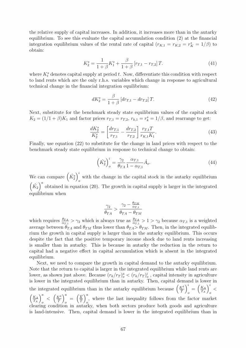
the relative supply of capital increases. In addition, it increases more than in the autarkyequilibrium. To see this evaluate the capital accumulation condition (2) at the financialintegration equilibrium values of the rental rate of capital (rK,1 = rK,2 = r∗K = 1/β) toobtain:

Ks2 =

1

1 + βKs

1 +β

1 + β[rT,1 − rT,2]T. (41)

where Kst denotes capital supply at period t. Now, differentiate this condition with respect

to land rents which are the only r.h.s. variables which change in response to agriculturaltechnical change in the financial integration equilibrium:

dKs2 =

β

1 + β[drT,1 − drT,2]T. (42)

Next, substitute for the benchmark steady state equilibrium values of the capital stockK2 = (1/1 + β)K1 and factor prices rT,1 = rT,2, rk,1 = r∗k = 1/β, and rearrange to get:

dKs2

Ks2

=

[drT,1rT,1

− drT,2rT,2

]rT,1T

rK,1K1

. (43)

Finally, use equation (22) to substitute for the change in land prices with respect to thebenchmark steady state equilibrium in response to technical change to obtain:(

Ks2

)io

=γ2

θTA

αT,11− αT,1

Ao. (44)

We can compare(Ks

2

)io

with the change in the capital stock in the autarky equilibrium(K2

)aobtained in equation (20). The growth in capital supply is larger in the integrated

equilibrium when

γ2

θTA>

γ2 − θTM

αT,1

θTA − θTMwhich requires θTA

αT,1> γ2 which is always true as θTA

αT,1> 1 > γ2 because αT,1 is a weighted

average between θTA and θTM thus lower than θTA> θTM . Then, in the integrated equilib-rium the growth in capital supply is larger than in the autarky equilibrium. This occursdespite the fact that the positive temporary income shock due to land rents increasingis smaller than in autarky. This is because in autarky the reduction in the return tocapital had a negative effect in capital accumulation which is absent in the integratedequilibrium.

Next, we need to compare the growth in capital demand to the autarky equilibrium.Note that the return to capital is larger in the integrated equilibrium while land rents arelower, as shown just above. Because (rk/rT )ao < (rk/rT )io , capital intensity in agricultureis lower in the integrated equilibrium than in autarky. Then, capital demand is lower in

the integrated equilibrium than in the autarky equilibrium because(Kd

T

)io

=(KA

TA

)io<(

KA

TA

)ao<(Kd

T

)ao

=(KT

)ao, where the last inequality follows from the factor market

clearing condition in autarky, when both sectors produce both goods and agricultureis land-intensive. Then, capital demand is lower in the integrated equilibrium than in

67

autarky. Then in the integrated equilibrium the growth in capital supply is larger than inautarky and the growth in capital demand is lower, thus there must be capital outflows.

Finally, we obtain the change in capital demand with respect to the benchmark equilib-rium. For this purpose, we make the simplifying assumption that the capital endowmentin the benchmark equilibrium is such that the origin economy is fully specialized in agricul-ture. This case is depicted in figure 2.b where the relative factor supply in the benchmark

equilibrium(KT

)io

intersects the relative factor demand in the agricultural sector at the

international factor prices (rk/rT )∗. We make this assumption to guarantee that the origineconomy is fully specialized in agriculture both in the benchmark equilibrium and whenthere is technical change. Otherwise, we would need to compare the full specializationequilibrium with one where the economy produces both goods and capital demand wouldnot change continuously.

To obtain the change in capital demand, note that equilibrium capital intensity inagriculture is given by:

KA

TA=aKA(rT , rK)

aTA(rT , rK).

Then, in an equilibrium with full specialization in agriculture capital demand is givenby:

Kd =aKA(rT , rK)

aTA(rT , rK)T .

where we used the factor market clearing condition in the land market. Log-differentiating,we obtain:

Kd = ˆaKA − ˆaTA = θTAσA (rT ) + θKAσA (rT ) = σA (rT ) ,

where the second equality uses the cost minimization conditions (12) to (15). Finally, wesubstitute for the change in land prices and get the equilibrium change in capital demand:(

Kd)io

=(1− γ2)

θTAσAAo.

As we have shown above, growth in capital demand is smaller in the integrated equilibriumthan in autarky. At the same time, the growth in capital supply is larger. Thus, there arecapital outflows. Here we also show that capital outflows are increasing in agriculturalproductivity growth:(

Ks)io−(Kd)io

=

[αT,1

1− αT,1γ2 − σA (1− γ2)

]AoθTA

. (45)

Thus, capital outflows are increasing in A if

αT,11− αT,1

γ2

(1− γ2)> σA,

that is, the land income share is large, the shock is temporary, and the elasticity ofsubstitution between land and capital in agricultural production is low.

68

Destination Region Finally, we consider a destination region which is open to inter-national trade but does not experience technical change. First, note that because theorigin region is a small economy, it does not affect international goods prices nor theinternational rental price of capital. As a result, if the destination region was in financialautarky or open to international capital flows, technical change in the origin would nothave any effect on the destination region. Then, we consider the more interesting casein which the two regions are financially integrated but in financial autarky with respectto the rest of the world. The equilibrium in the destination region is depicted in Figure3. First, note that because the destination region did not experience technical change,factor prices stay at the level (rk/rT )∗ given by initial technology and international goodsprices. As a result, the equilibrium in the origin region is the same as if it was integratedin international capital markets, depicted in Figure 2. This is because capital leaving theorigin region can flow in the destination region without affecting the rental rate of capital.Instead, the destination region absorbs this additional capital by expanding production ofthe capital-intensive sector, manufacturing. This is because this destination region facesa pure Rybzcinsky effect with no changes in technology. To see this, log-differentiate thethe factor market clearing conditions (6) and (7) in the destination region to find thatthe expansion in manufacturing output in the destination region is proportional to thegrowth in capital supply: (

XM − XA

)id

=1

λKM − λTM

(Ks)id, (46)

where hats denote percent changes of the variables of interest in the destination regionin the integrated equilibrium with respect to the benchmark equilibrium where no regionfaces technical change. Then, because all the increase in capital supply in the destinationregion comes from capital outflows in the origin region (∆Ks

d = ∆Kso −∆Kd

o ) the growthin capital supply in the destination region in the integrated equilibrium is(

K)id

= ωod

(Kso − Kd

o

)io

(47)

where ωod = Ko/Kd is the ratio of capital stocks in the benchmark equilibrium. Thus,(XM − XA

)id

=1

λKM − λTMωod

(Kso − Kd

o

)io, (48)

Finally, the change in the share of capital allocated to manufacturing is λKM = XM −Kwhich yields (

λKM

)id

=1− (λKM − λTM)

λKM − λTM

(K)id. (49)

69

B Empirics: Derivations

This Appendix presents the derivations to obtain the estimates of bank exposure andmunicipality exposure to the GE soy driven deposit increase presented in equations (13)and (14) respectively in the paper.

B.A From Model to Data

In the model, there are only two regions which are financially integrated with eachother and in autarky with respect to the rest of the world. In this case, agriculturaltechnical change generates capital outflows from the origin to the destination region equalto the difference between the growth in capital supply and capital demand in the originregion [see equation (8)]. Recall that these capital inflows do not generate changes in thereturn to capital in the destination region because free trade in goods implies that factorprices are pinned down by international goods prices. Note that the return to capital beingconstant in the destination region implies that it is also constant in the origin region dueto financial integration. Thus, our empirical analysis will focus on tracking capital flowsacross regions taking interest rates as given. In the data there are several regions and wecan only track capital flows which are intermediated through banks. Thus, we adapt themodel’s prediction to our context by introducing banks and many regions.

We think of banks as intermediaries that can reallocate savings from depositors tofirms. The role of banks as intermediaries has been justified due to their advantage inmonitoring firms in the context of asymmetric information (Diamond 1984, Holmstromand Tirole 1997). As our main objective is to use banks to measure the degree of financialintegration across regions, we do not explicitly provide for micro-foundations of the roleof banks here. Instead, we extend our model in the simplest possible way by assumingthat banks are providers of a technology that permits to reallocate capital across regionswhere the same bank has branches, in the same way as transportation technology permitsto trade goods across regions connected by a road.

B.A.1 Savings and deposits in origin municipalities

First, we assume that local savings are deposited in local banks. Second, we assumethat each bank has a constant market share in each local deposit market (ψbo). Thus,we can write depositsbo = ψboK

so . This implies that savings deposits in each local bank

branch grow at the same rate as local aggregate savings. Thus by using equation (6) weobtain:

ˆdepositsbo =(Ks)io

= φToAo. (50)

where depositsbo are local deposits of bank b in origin municipality o and φTo =[γ2θTA

αT,1

1−αT,1

]is increasing in the land income share at the origin municipality αT,1 as all remaining vari-ables are identical for all municipalities due to factor price equalization in the benchmarkequilibrium. Next, we would like to obtain an expression for the increase in nationaldeposits of each bank due to technical change in soy. For this purpose, first note that,for each bank b, national deposits can be obtained by aggregating deposits collected inall municipalities where the bank has branches:

70

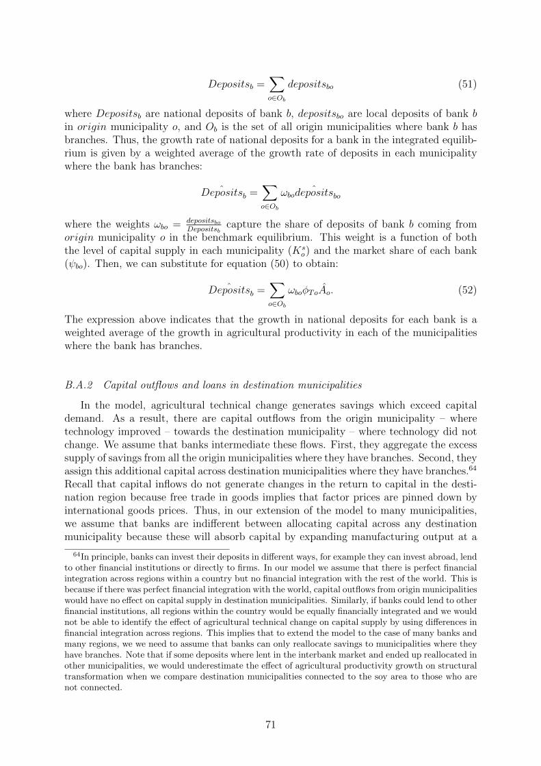
Depositsb =∑o∈Ob

depositsbo (51)

where Depositsb are national deposits of bank b, depositsbo are local deposits of bank bin origin municipality o, and Ob is the set of all origin municipalities where bank b hasbranches. Thus, the growth rate of national deposits for a bank in the integrated equilib-rium is given by a weighted average of the growth rate of deposits in each municipalitywhere the bank has branches:

ˆDepositsb =∑o∈Ob

ωbo ˆdepositsbo

where the weights ωbo = depositsboDepositsb

capture the share of deposits of bank b coming fromorigin municipality o in the benchmark equilibrium. This weight is a function of boththe level of capital supply in each municipality (Ks

o) and the market share of each bank(ψbo). Then, we can substitute for equation (50) to obtain:

ˆDepositsb =∑o∈Ob

ωboφToAo. (52)

The expression above indicates that the growth in national deposits for each bank is aweighted average of the growth in agricultural productivity in each of the municipalitieswhere the bank has branches.

B.A.2 Capital outflows and loans in destination municipalities

In the model, agricultural technical change generates savings which exceed capitaldemand. As a result, there are capital outflows from the origin municipality – wheretechnology improved – towards the destination municipality – where technology did notchange. We assume that banks intermediate these flows. First, they aggregate the excesssupply of savings from all the origin municipalities where they have branches. Second, theyassign this additional capital across destination municipalities where they have branches.64

Recall that capital inflows do not generate changes in the return to capital in the desti-nation region because free trade in goods implies that factor prices are pinned down byinternational goods prices. Thus, in our extension of the model to many municipalities,we assume that banks are indifferent between allocating capital across any destinationmunicipality because these will absorb capital by expanding manufacturing output at a

64In principle, banks can invest their deposits in different ways, for example they can invest abroad, lendto other financial institutions or directly to firms. In our model we assume that there is perfect financialintegration across regions within a country but no financial integration with the rest of the world. This isbecause if there was perfect financial integration with the world, capital outflows from origin municipalitieswould have no effect on capital supply in destination municipalities. Similarly, if banks could lend to otherfinancial institutions, all regions within the country would be equally financially integrated and we wouldnot be able to identify the effect of agricultural technical change on capital supply by using differences infinancial integration across regions. This implies that to extend the model to the case of many banks andmany regions, we we need to assume that banks can only reallocate savings to municipalities where theyhave branches. Note that if some deposits where lent in the interbank market and ended up reallocated inother municipalities, we would underestimate the effect of agricultural productivity growth on structuraltransformation when we compare destination municipalities connected to the soy area to those who arenot connected.

71

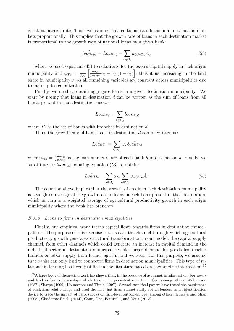
constant interest rate. Thus, we assume that banks increase loans in all destination mar-kets proportionally. This implies that the growth rate of loans in each destination marketis proportional to the growth rate of national loans by a given bank:

ˆloansbd = ˆLoansb =∑o∈Ob

ωboϕToAo. (53)

where we used equation (45) to substitute for the excess capital supply in each origin

municipality and ϕTo = 1θTA

[αT,1

1−αT,1γ2 − σA (1− γ2)

], thus it us increasing in the land

share in municipality o, as all remaining variables are constant across municipalities dueto factor price equalization.

Finally, we need to obtain aggregate loans in a given destination municipality. Westart by noting that loans in destination d can be written as the sum of loans from allbanks present in that destination market:

Loansd =∑b∈Bd

loansbd

where Bd is the set of banks with branches in destination d.Thus, the growth rate of bank loans in destination d can be written as:

ˆLoansd =∑b∈Bd

ωbd ˆloansbd

where ωbd = loansbdloansd

is the loan market share of each bank b in destination d. Finally, we

substitute for ˆloansbd by using equation (53) to obtain:

ˆLoansd =∑b∈Bd

ωbd∑o∈Ob

ωboϕToAo. (54)

The equation above implies that the growth of credit in each destination municipalityis a weighted average of the growth rate of loans in each bank present in that destination,which in turn is a weighted average of agricultural productivity growth in each originmunicipality where the bank has branches.

B.A.3 Loans to firms in destination municipalities

Finally, our empirical work traces capital flows towards firms in destination munici-palities. The purpose of this exercise is to isolate the channel through which agriculturalproductivity growth generates structural transformation in our model, the capital supplychannel, from other channels which could generate an increase in capital demand in theindustrial sector in destination municipalities like larger demand for goods from richerfarmers or labor supply from former agricultural workers. For this purpose, we assumethat banks can only lend to connected firms in destination municipalities. This type of re-lationship lending has been justified in the literature based on asymmetric information.65

65A large body of theoretical work has shown that, in the presence of asymmetric information, borrowersand lenders form relationships which tend to be persistent over time. See, among others, Williamson(1987), Sharpe (1990), Holmstrom and Tirole (1997). Several empirical papers have tested the persistenceof bank-firm relationships and used the fact that firms cannot easily switch lenders as an identificationdevice to trace the impact of bank shocks on firm-level outcomes. See, among others: Khwaja and Mian(2008), Chodorow-Reich (2014), Cong, Gao, Ponticelli, and Yang (2018).

72

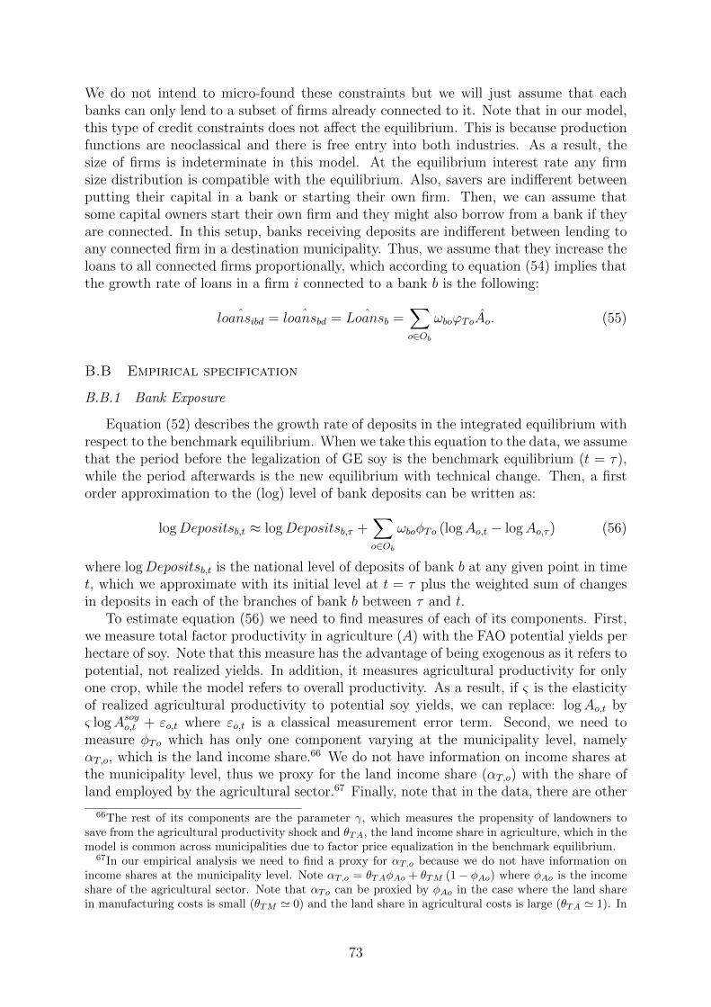
We do not intend to micro-found these constraints but we will just assume that eachbanks can only lend to a subset of firms already connected to it. Note that in our model,this type of credit constraints does not affect the equilibrium. This is because productionfunctions are neoclassical and there is free entry into both industries. As a result, thesize of firms is indeterminate in this model. At the equilibrium interest rate any firmsize distribution is compatible with the equilibrium. Also, savers are indifferent betweenputting their capital in a bank or starting their own firm. Then, we can assume thatsome capital owners start their own firm and they might also borrow from a bank if theyare connected. In this setup, banks receiving deposits are indifferent between lending toany connected firm in a destination municipality. Thus, we assume that they increase theloans to all connected firms proportionally, which according to equation (54) implies thatthe growth rate of loans in a firm i connected to a bank b is the following:

ˆloansibd = ˆloansbd = ˆLoansb =∑o∈Ob

ωboϕToAo. (55)

B.B Empirical specification

B.B.1 Bank Exposure

Equation (52) describes the growth rate of deposits in the integrated equilibrium withrespect to the benchmark equilibrium. When we take this equation to the data, we assumethat the period before the legalization of GE soy is the benchmark equilibrium (t = τ),while the period afterwards is the new equilibrium with technical change. Then, a firstorder approximation to the (log) level of bank deposits can be written as:

logDepositsb,t ≈ logDepositsb,τ +∑o∈Ob

ωboφTo (logAo,t − logAo,τ ) (56)

where logDepositsb,t is the national level of deposits of bank b at any given point in timet, which we approximate with its initial level at t = τ plus the weighted sum of changesin deposits in each of the branches of bank b between τ and t.

To estimate equation (56) we need to find measures of each of its components. First,we measure total factor productivity in agriculture (A) with the FAO potential yields perhectare of soy. Note that this measure has the advantage of being exogenous as it refers topotential, not realized yields. In addition, it measures agricultural productivity for onlyone crop, while the model refers to overall productivity. As a result, if ς is the elasticityof realized agricultural productivity to potential soy yields, we can replace: logAo,t byς logAsoyo,t + εo,t where εo,t is a classical measurement error term. Second, we need tomeasure φTo which has only one component varying at the municipality level, namelyαT,o, which is the land income share.66 We do not have information on income shares atthe municipality level, thus we proxy for the land income share (αT,o) with the share ofland employed by the agricultural sector.67 Finally, note that in the data, there are other

66The rest of its components are the parameter γ, which measures the propensity of landowners tosave from the agricultural productivity shock and θTA, the land income share in agriculture, which in themodel is common across municipalities due to factor price equalization in the benchmark equilibrium.

67In our empirical analysis we need to find a proxy for αT,o because we do not have information onincome shares at the municipality level. Note αT,o = θTAφAo + θTM (1− φAo) where φAo is the incomeshare of the agricultural sector. Note that αTo can be proxied by φAo in the case where the land sharein manufacturing costs is small (θTM ' 0) and the land share in agricultural costs is large (θTA ' 1). In

73

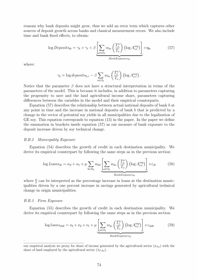
reasons why bank deposits might grow, thus we add an error term which captures othersources of deposit growth across banks and classical measurement errors. We also includetime and bank fixed effects, to obtain:

logDepositsbt = γb + γt + β

[∑o∈Ob

wbo

(T aoTo

)(logAsoyo,t

)]︸ ︷︷ ︸

BankExposurebt

+ηbt (57)

where:

γb = log depositsb,τ − β∑o∈Ob

wbo

(T aoTo

)(logAsoyo,τ

).

Notice that the parameter β does not have a structural interpretation in terms of theparameters of the model. This is because it includes, in addition to parameters capturingthe propensity to save and the land agricultural income share, parameters capturingdifferences between the variables in the model and their empirical counterparts.

Equation (57) describes the relationship between actual national deposits of bank b atany point in time and the increase in national deposits of bank b that is predicted by achange in the vector of potential soy yields in all municipalities due to the legalization ofGE soy. This equation corresponds to equation (13) in the paper. In the paper we definethe summation in brackets inside equation (57) as our measure of bank exposure to thedeposit increase driven by soy technical change.

B.B.2 Municipality Exposure

Equation (54) describes the growth of credit in each destination municipality. Wederive its empirical counterpart by following the same steps as in the previous section:

logLoansdt = αd + αt + µ∑b∈Bd

wbd

[∑o∈Ob

wbo

(T aoTo

)(logAsoyo,t

)]︸ ︷︷ ︸

BankExposurebt

+εdt (58)

where µβ

can be interpreted as the percentage increase in loans at the destination munic-ipalities driven by a one percent increase in savings generated by agricultural technicalchange in origin municipalities.

B.B.3 Firm Exposure

Equation (55) describes the growth of credit in each destination municipality. Wederive its empirical counterpart by following the same steps as in the previous section:

log loansibdt = νb + νd + νt + µ

[∑o∈Ob

wbo

(T aoTo

)(logAsoyo,t

)]︸ ︷︷ ︸

BankExposurebt

+εibdt (59)

.

our empirical analysis we proxy for share of income generated by the agricultural sector (φAo) with theshare of land employed by the agricultural sector (λTAo).

74

where µβ

can be interpreted as the percentage increase in loans at the destination

municipalities driven by a one percent increase in aggregate savings (deposits) generatedby agricultural technical change in origin municipalities.

75