RESEARCH PAPER

Capillary rise method for the measurement of the contact angleof soils

Zhen Liu • Xiong Yu • Lin Wan

Received: 17 November 2013 / Accepted: 27 August 2014

� Springer-Verlag Berlin Heidelberg 2014

Abstract The contact angle quantitatively describes the

contact on the liquid–solid interface and is thus critical to

many physical processes involving interactions between

soils and water. However, the role of the contact angle in

soils is far from being adequately recognized. This paper

reports a comprehensive study on the application of the

capillary rise method (CRM) to measure the contact angles

of soils. The deviations of analytical solutions to various

forms of the Lucas–Washburn equation were presented to

offer a detailed study on the theoretical basis for applying

CRM to soils, which is absent in existing studies. The

disadvantages of the conventional CRM investigations

were demonstrated with experiments. Based on a com-

parative study, a modified CRM was proposed based on the

analytical solution to one form of the Lucas–Washburn

equation. This modified CRM exhibited a reliable perfor-

mance on numerous unsieved and sieved (different average

particle sizes) specimens made of a subgrade soil and a

silicon dioxide sand. Procedures for the specimen

preparation were designed and strictly followed, and

innovative apparatuses for the preparation, transport, and

accommodation of soil specimens were fabricated to

ensure repeatability. For the modified CRM, experimental

results for unsieved specimens exhibited good repeatabil-

ity, while for sieved soils, clear trends were observed in the

variations of the contact angle with particle size. Contact

angles much greater than zero were observed for all of the

tested soil specimens. The results indicate that the

assumption of perfect wettability, which is adopted in

many existing geotechnical studies involving the contact

angle, is unrealistic.

Keywords Capillary rise method � Contact angle �Lucas–Washburn equation � Soil water characteristic curve

1 Introduction

The contact angle, or more specifically, the angle between

liquid–gas and liquid–solid interfaces, is an intrinsic

property of solid–liquid–gas systems such as soils [36]. It is

of great significance in many soil physical processes

involving the interaction between soil and water [3, 14].

For example, it is critical to water infiltration, redistribu-

tion, groundwater recharge, solute transport in unsaturated

zones, compaction and aeration in variably saturated soils,

and temperature-induced water redistribution [5, 24]. This

is because this property quantifies the ability of a liquid to

spread on another solid [32]. Taking the soil water char-

acteristic curve (SWCC) for example, this key relationship

in unsaturated soil mechanics depends on both the soil

matrix tomography (i.e., pore-size distribution) and surface

physical chemistry (i.e., contact angle). While the pore-size

distribution has been extensively studied for SWCCs, the

Z. Liu

Department of Civil Engineering and Environmental

Engineering, Michigan Technological University,

1400 Townsend Drive, Dillman 201F, Houghton,

MI 49931, USA

e-mail: zhenl@mtu.edu

X. Yu (&)

Department of Civil Engineering, Case Western Reserve

University, 10900 Euclid Avenue, Bingham 206, Cleveland,

OH 44106-7201, USA

e-mail: xxy21@case.edu

L. Wan

Department of Civil Engineering, Case Western Reserve

University, 10900 Euclid Avenue, Bingham 259, Cleveland,

OH 44106-7201, USA

e-mail: lin.wan@case.edu

123

Acta Geotechnica

DOI 10.1007/s11440-014-0352-x

contact angle is usually assumed to be a constant, mostly

zero, for simplicity in view of the high surface energy of

soil minerals [4, 5, 18]. However, despite a few investi-

gations into the effect of the contact angle [34], these

assumptions of a constant (or zero) contact angle corre-

sponding to an invariant (or perfect) wettability, especially

in a wetting process, have rarely been validated by

experimental evidence. In fact, a varying contact angle

value (nonzero) with respect to various factors, such as

water potential, roughness, and temperature, has been fre-

quently reported by the outsiders of geotechnical engi-

neering, such as soil scientists, agricultural engineers, and

physical chemists [15, 22, 23, 46, 47].

Various methods have been proposed for the mea-

surement of the contact angles of soils on the basis of

different mechanisms, e.g., the water drop penetration

time [13, 31, 40], the molarity of an ethanol droplet [12,

28], and the flotation time [43, 49]. More recently, the

CRM [2], the sessile drop method [6] and Wilhelmy plate

method [7] have been developed for soils. Among these

methods, the CRM based on the Lucas–Washburn equa-

tion [38, 59] is by nature suitable for hydrophilic soils,

which exactly cover the soils affiliated with SWCCs in

geotechnical engineering. One distinct advantage of this

method is that it is capable of assessing the average

contact angle of a bulk of soil rather than that of several

layers of the soil close to the surface. This average contact

angle which is essentially the average apparent contact

angle is different from the intrinsic contact angle between

water and a flat smooth mineral interface. Instead, it

represents the average contact angle of a conceptualized

bundle of cylindrical capillaries (BCC) [57], which is also

the conceptual model used by most SWCC formulations.

Therefore, the CRM is by nature suitable for porous

materials such as soils.

Despite the development of the Lucas–Washburn

equation since 1920s [38, 59], the CRM for porous mate-

rials based on this equation had not been extensively

investigated until 1990s [2]. Due to this reason, there are

only a few attempts at applying this type of method to soils.

The earliest effort was the study of Letey et al. [32] on the

measurement of liquid–solid contact angles in soils based

on both Poiseuille’s approximation and the force balance

for infiltration into soil, which were equivalent to the

Lucas–Washburn equation. Siebold et al. [53] applied the

CRM to silica flour and calcium carbonate by measuring

both the height (by a scale) and mass (by Kruss 12 tensi-

ometer) of imbibed liquids. Michel et al. [41] measured the

wettability of partly decomposed peats with a Kruss 12

tensiometer based on the CRM, in which the tortuosity of

the capillaries was considered. Abu-Zreig et al. [1] made a

simple application of the CRM for measuring the contact

angles between soils and various test liquids while studying

the effect of surfactants on hydraulic properties of soils.

Geobel et al. [22] claimed their study to be the first one that

applied the CRM to soil aggregates. In this study, the

masses of imbibed liquids were measured with an elec-

tronic balance, and details in experiment setup and influ-

encing factors were discussed. Ramirez-Flores et al. [47]

followed Goebel’s method [22] for measuring the contact

angles of intact soil aggregates, packing of intact aggre-

gates, and packing of crushed aggregates of nine topsoils

and three humus subsoils.

A recent publication of the authors [35] reported that

the contact angle may play a significant role in unsatu-

rated soils via the SWCC. And a modified way for

implementing CRM was briefly introduced, but not

detailed. This study presents a comprehensive study for

applying the CRM to the contact angle measurement of

hydrophilic soils. The deviations of analytical solutions to

various forms of the Lucas–Washburn equation were

presented to offer a detailed study on the theoretical basis

for applying the CRM to soils, which is absent in existing

studies. Measures were taken to overcome several diffi-

culties, preventing accurate contact angle measurements

with the CRM: (1) a self-fabricated tube with special

design to eliminate external meniscus; (2) specially

designed soil specimen preparation procedures to ensure

consistency in sample qualities and repeatability of

experiments; and (3) automatic data processing to avoid

subjective factors. A comparative study is conducted to

evaluate several different ways for implementing the

CRM, which includes the one used by most of the

existing studies. A modified CRM method is suggested

and validated based on the comparative study. Contact

angles were measured for the specimens made of two

typical soils, either sieved or unsieved. This pioneering

study will provide a complete and detailed reference for

later investigations into the contact angle of soils, espe-

cially those using the CRM, which are expected to be

boomed as the significant role of the contact angle is

more and more clearly realized.

2 Theory

There are four types of forces involved in the dynamic

process of a capillary rise in a cylindrical tube or a capil-

lary. These forces include surface tension, inertial force,

viscous force, and gravity. Thus, the governing equation is

obtained by ensuring the equilibrium of imbibed water by

allowing for these forces (Eq. 1) [27, 62].

Acta Geotechnica

123

2prc cos hð Þ|fflfflfflfflfflfflffl{zfflfflfflfflfflfflffl}

Surface Tension

� qpr2 o

oth tð Þ oh tð Þ

ot

� �

|fflfflfflfflfflfflfflfflfflfflfflfflfflfflffl{zfflfflfflfflfflfflfflfflfflfflfflfflfflfflffl}

Inertial Force

� 8pgh tð Þ oh tð Þot

|fflfflfflfflfflfflfflfflffl{zfflfflfflfflfflfflfflfflffl}

Viscous Force

� qpr2gh tð Þ|fflfflfflfflfflffl{zfflfflfflfflfflffl}

Gravity

¼ 0 ð1Þ

where the four terms on the left-hand side represent surface

tension, inertial force, viscous force and gravity,

respectively; r is the radius of the tube; c is the surface

tension of the interface between the test (imbibed) liquid

and gas; h is the contact angle; t is time; h(t) is the height of

the capillary rise at time t; g and q are the dynamic

viscosity and density of the test liquid, respectively; and g

is the gravitational acceleration. The positive or negative

sign in front of a term indicates the corresponding force is a

motivation or a resistance to the capillary rise. This

equation was developed based on the following

assumptions [19]. (1) The flow is one-dimensional. (2)

There is no friction or inertia effect caused by displaced air.

(3) There is no inertia or entry effect in the liquid reservoir.

(4) The viscous pressure loss inside the tube is given by the

Hagen–Poiseuille law. Equation 1 strictly describes the

variation of the capillary height with time once all the

assumptions are ensured. This equation can be simplified as

Eq. 2.

B� A hh0ð Þ0�Chh0 � Dh ¼ 0 ð2Þ

where A ¼ qpr2; B ¼ 2prc cos hð Þ; C ¼ 8pg; and

D ¼ qpr2g.

Equation 1 is the most up-to-date form of the Lucas–

Washburn equation based on modifications to the original

ones with and without gravity [51]. The Lucas–Washburn

equation was designated to describe the dynamics of a

capillary rise in a single cylindrical capillary or tube. When

extending this equation to porous materials such as soils,

the porous medium is conceptualized as a BCC. This

conceptual model of a BCC of different radii has also been

frequently used in unsaturated soil mechanics for the

development of SWCCs. For the dynamics of the capillary

rise, the original BCC of different radii was then equiva-

lently viewed as another bundle of capillaries of an iden-

tical radius [33]. This radius is called the effective radius

(or average radius). The Lucas–Washburn equation is

assumed to be valid for the capillary rise in every capillary

within the equivalent bundle.

There is a unique solution to the above ordinary dif-

ferential equation (ODE) once the porous material (r) and

test liquid (q,g) are determined (h is dependent on both the

porous material and the test liquid). But unfortunately,

there is no analytical solution available for the above ODE.

And our preliminary study indicated that direct curve fit-

ting with the above ODE to experimental data requires a

capacity of optimization that is far beyond what is currently

available. So, in the current stage, a feasible strategy is to

obtain an analytical solution to a simplified form of the

above complete Lucas–Washburn equation and then to

perform curve fitting with the analytical solution to the

simplified form. This is actually the strategy used by the

aforementioned CRM studies. Depending on the simplifi-

cations employed, four methods for implementing the

CRM can be obtained, which will be introduced in the

following subsections.

2.1 CRM without gravity and inertia (method 1)

The influences of inertia and gravity were neglected in

most of the existing CRM studies. Consequently, a sim-

plified Lucas–Washburn equation which is familiar to

researchers can be obtained in the following form.

2prc cos hð Þ|fflfflfflfflfflfflffl{zfflfflfflfflfflfflffl}

Surface Tension

� 8pgh tð Þ oh tð Þot

|fflfflfflfflfflfflfflfflffl{zfflfflfflfflfflfflfflfflffl}

Viscous Force

¼ 0 B� Chh0 ¼ 0ð Þ ð3Þ

The analytical solution to this simplified Lucas–Washburn

equation predicts a linear relationship between the squared

height of imbibed liquid and time [2, 59]. This analytical

solution can then be used for curve fitting to compute the

contact angle.

h ¼ 2B

Ct

� �1=2

¼ rc cos h2g

t

� �1=2

ð4Þ

It is possible that the height of the liquid front is not visible

or that the liquid front does not accurately reflect the inner

progression of the liquid in the porous material. Hence, the

above solution (height gain) is reformatted into the form of

imbibed mass (mass gain). An equivalent equation was

then obtained, which was used by most CRM studies [53].

Here we formulate the equation in the following way to be

consistent with the BCC theory.

m ¼ p2r5N � q2c

2g� cos h � t

� �1=2

ð5Þ

where N is the number of equivalent capillaries in a cap-

illary rise process, and p2r5N is usually referred to as

Washburn constant. Stange [54] and Fries and Dreyer [20]

believed that the very first stage was purely dominated by

inertial forces, and subsequently the influence of viscosity

increases (visco-inertial flow). After that, the effect of

inertia vanishes and the flow becomes purely viscous. This

viscosity-dominant period corresponds to a mechanism

described by Eqs. 3–5. But the influence of gravity has

been proven to be significant when height of the capillary

reaches one-tenth of the equilibrium height [20]. So the

application of this method requires identifying a stage

Acta Geotechnica

123

when the above equation can satisfactorily describe the

dynamics of the capillary rise. However, it is possible that

such a stage is very short or even does not evidently exist.

Even if there exists such a stage, a segment of the m2–

t curve whose tangent has the least slope variation needs to

be identified for a subsequent linear regression to deter-

mine the contact angle [53]. Thus, the implementation of

the method could be very subjective. These two concerns

were investigated by experiments and will be introduced

later in this study.

2.2 CRM without gravity (method 2)

As mentioned, no explicit solution to the complete Lucas–

Washburn equation is available by now. Nonetheless, the

simplified Washburn equation used by Method 1 can still be

improved by taking into account the inertial force. This

consequent equation (Eq. 6) is possibly able to provide a

good prediction for the capillary rise, especially when the

height of water front is much less than the equilibrium height.

2prc cos hð Þ|fflfflfflfflfflfflffl{zfflfflfflfflfflfflffl}

Surface Tension

� qpr2 o

oth tð Þ oh tð Þ

ot

� �

|fflfflfflfflfflfflfflfflfflfflfflfflfflfflffl{zfflfflfflfflfflfflfflfflfflfflfflfflfflfflffl}

Inertial Force

� 8pgh tð Þ oh tð Þot

|fflfflfflfflfflfflfflfflffl{zfflfflfflfflfflfflfflfflffl}

Viscous Force

¼ 0

B� A hh0ð Þ0�Chh0 ¼ 0� �

ð6Þ

An explicit analytical solution to the above equation is

possible and can be formulated as Eq. 7.

h ¼ C1

A� C1

Aexp �C

At

� �

þ 2B

Ct

� �1=2

¼ C1

qpr2� C1

qpr2exp � 8g

qr2t

� �

þ rc cos h2g

t

� �1=2

ð7Þ

where C1 is a constant. The solution could be reformatted

to describe the variation of mass as Eq. 8.

m ¼ C1qpr2N � C1qpr2N exp � 8gqr2

t

� ��

þp2r5N � q2c

2g� cos h � t

�1=2

ð8Þ

It is the first time an analytical solution to this form of

Lucas–Washburn equation is obtained. Therefore, this

solution has never been used in previous CRM studies. Its

application to CRM was also tested by experiments in this

study.

2.3 CRM without inertia (method 3)

Alternatively, the influence of gravity instead of inertia

could be considered as Eq. 9. This equation is valid as long

as the effect of inertia is negligible.

2prc cos hð Þ|fflfflfflfflfflfflffl{zfflfflfflfflfflfflffl}

Surface Tension

� 8pgh tð Þ oh tð Þot

|fflfflfflfflfflfflfflfflffl{zfflfflfflfflfflfflfflfflffl}

Viscous Force

� qpr2gh tð Þ|fflfflfflfflfflffl{zfflfflfflfflfflffl}

Gravity

¼ 0

B� Chh0 � Dh ¼ 0ð Þ

ð9Þ

The analytical solution could be obtained using

MATLAB.

h ¼ B

D1� 1

exp x �1� D2

BCt

� �

exp 1þ D2

BCt

� �

( )

ð10Þ

where x represents the Wright Omega function. This

equation can be further reduced to Eq. 11. Fries and Dreyer

[19] obtained a similar equation in a different way.

h ¼ B

D1�W exp �1� D2

BCt

� �� �� �

ð11Þ

where W is the Lambert W function. That is,

h ¼ 2c cos hð Þqgr

1�W exp �1� q2g2r3

16cg cos hð Þ t� �� �� �

ð12Þ

The solution is reformatted to describe the variation of

mass.

m ¼ 2prNc cos hð Þg

1�W exp �1� q2g2r3

16cg cos hð Þ t� �� �� �

ð13Þ

The Lambert W function cannot be expressed in terms of

elementary functions. The piecewise equation proposed by

Barry et al. [8] was used to approximate this equation in

this study. An alternative is to use the Taylor series of the

above equation around 0 based on the Lagrange inversion

theorem as follows,

m ¼ 2prNc cos hð Þg

1�X1

n¼0

�n� 1ð Þn

nþ 1ð Þ!

�(

� 1

enexp � q2g2r3

16cg cos hð Þ nt

� ��)

ð14Þ

where e is the base of natural logarithm.

2.4 Application to porous materials

Czachor [10] claimed that two features of porous materials

should be responsible for the overestimations of the contact

angle by applying the Lucas–Washburn equation to porous

materials: cross section and tortuosity. But according to the

definition of the apparent contact angle of porous materials

Acta Geotechnica

123

[25, 42], the intergranular characteristic has already been

taken into account. The contact angle of a porous medium

measured with the CRM is the apparent contact angle

considering roughness. The effects of the roughness of

internal pores on the difference between the apparent

contact angle and intrinsic contact angle (Young’s contact

angle) have been extensively discussed [9, 15, 30, 46, 48,

50, 55]. However, tortuosity was not included in the defi-

nition of the apparent contact angle. As the result, the

influence of tortuosity on the applications of the CRM

based on the Lucas–Washburn equation to measure the

apparent contact angle of porous materials deserves close

attention. According to Czachor [11], the tortuosity s is

defined as the ratio of the actual path taken by a moving

liquid through pores, ~h, and the distance between the start

and final heights, h [17, 52, 58].

~h ¼ sh ð15Þ

The Lucas–Washburn equation taking into account

tortuosity of the porous material is as Eq. 16.

2p~rc cos ~h �

|fflfflfflfflfflfflfflffl{zfflfflfflfflfflfflfflffl}

Surface Tension

� qp~r2 o

ot~h tð Þ o

~h tð Þot

� �

|fflfflfflfflfflfflfflfflfflfflfflfflfflfflffl{zfflfflfflfflfflfflfflfflfflfflfflfflfflfflffl}

Inertial Force

� 8pg~h tð Þ o~h tð Þot

|fflfflfflfflfflfflfflfflffl{zfflfflfflfflfflfflfflfflffl}

Viscous Force

� qp~r2g~h tð Þ|fflfflfflfflfflffl{zfflfflfflfflfflffl}

Gravity

¼ 0 ð16Þ

where ~r and ~h are the effective pore radius and the contact

angle considering tortuosity, respectively. Their values

may differ from those obtained by fitting experimental data

with the original Lucas–Washburn equation. Equation 16

needs to be transformed in terms of the apparent rise of

capillary instead of the actual path as Eq. 17 to take

advantage of measured data.

2p~rc cos ~h �

|fflfflfflfflfflfflfflffl{zfflfflfflfflfflfflfflffl}

Surface Tension

� qp~r2s2 o

oth tð Þ oh tð Þ

ot

� �

|fflfflfflfflfflfflfflfflfflfflfflfflfflfflfflfflffl{zfflfflfflfflfflfflfflfflfflfflfflfflfflfflfflfflffl}

Inertial Force

� 8pgs2h tð Þ oh tð Þot

|fflfflfflfflfflfflfflfflfflfflffl{zfflfflfflfflfflfflfflfflfflfflffl}

Viscous Force

� qp~r2gsh tð Þ|fflfflfflfflfflfflffl{zfflfflfflfflfflfflffl}

Gravity

¼ 0 ð17Þ

Equation 17 can be simplified as Eq. 18.

~B� ~A hh0ð Þ0� ~Chh0 � ~Dh ¼ 0 ð18Þ

where ~A ¼ qp~r2s2, ~B ¼ 2p~rc cos ~h �

, ~C ¼ 8pgs2, and

~D ¼ qp~r2gs. In fact, the values of ~A, ~B, ~C and ~D are equal

to those of A, B, C and D, respectively, from curve fitting,

but here we use different notations to indicate the different

physical meanings.

Based on the above discussion, it is clear that the fitting

functions derived in 2.1, 2.2 and 2.3 need to be adjusted to

allow for tortuosity prior to applications. The adjusted

governing equations (ODEs), fitting functions, and desired

fitting constants containing the contact angle for height gain

and mass gain, respectively, are summarized in Table 1.

The fitting functions were summarized in the following way

to achieve a unified framework to integrate and compare the

different models that are currently available. The fitting

constant, jJ (J = 1, 2, 3), was chosen because it contains all

the unknowns, and also because, in such a way this study

could be consistent with the existing CRM studies.

Gurau and Mann [26] proposed a fitting function for using

the CRM to characterize the wettability of gas diffusion

media for proton exchange membrane in fuel cells. This

equation, which is an extension to Method 1 by allowing for

the influence of the external meniscus and the mass absorbed

on the balance before measurements, yielded satisfactory

results in their study. This fitting equation was evaluated as

Method 4 in the comparative study introduced later.

m ¼ m0 þ a4 tanh b4tð Þ þ j4tð Þ1=2 Method 4ð Þ ð19Þ

where m0 is the mass absorbed on the balance, and the

second term was used to describe the mass increase caused

by the external meniscus. A term similar to m0 was added

to the fitting functions of Methods 1, 2, and 3 in the fol-

lowing analyses.

3 Materials and method

3.1 Method

Table 1 summarizes three fitting equations based on the

Lucas–Washburn equation including the simplified one

(Method 1) used by most existing studies for applying the

CRM in soils. Together with Method 4, these fitting

equations are adopted to fit measured m–t relationships

when using the CRM to measure apparent contact angles of

soils. For this purpose, constants in the fitting equations,

i.e., A, B, C, D, or their combinations such as jJ (J = 1, 2,

3 and 4) will be determined. Based on these constants,

there are two ways to obtain contact angles. One approach

is for height gain fitting functions only. Because the

effective radius and apparent contact angle are the two

unknowns, the apparent contact angle can be calculated

with an additional relationship between the effective radius

and the contact angle [61]. But more often, water and

another test liquid for reference are used for the second

approach. The employment of a reference liquid is neces-

sary for the weight gain fitting functions due to the exis-

tence of three unknowns. The reference liquid is usually an

organic solvent with low surface energy, such as hexane

and pentane. Pentane was used in this study. Considering

the comparatively high surface energy of soil particles and

low surface tension of the test liquid, the contact angle

between the test liquid and soils is approximately zero.

Acta Geotechnica

123

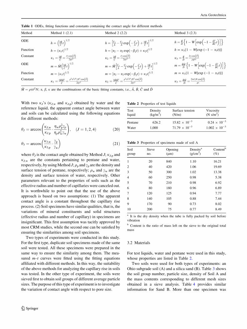
With two jJ’s (jJ,w and jJ,p) obtained by water and the

reference liquid, the apparent contact angle between water

and soils can be calculated using the following equations

for different methods:

hJ ¼ arccosjJ;w

jJ;p�gwq2

pcp

gpq2wcw

!

; J ¼ 1; 2; 4ð Þ ð20Þ

h3 ¼ arccosj3;w

j3;p�cp

cw

� �

ð21Þ

where hJ is the contact angle obtained by Method J; jJ,p and

jJ,w are the constants pertaining to pentane and water,

respectively, by using Method J; qp and cp are the density and

surface tension of pentane, respectively; qw and cw are the

density and surface tension of water, respectively. Other

parameters relevant to the properties of soils such as the

effective radius and number of capillaries were canceled out.

It is worthwhile to point out that the use of the above

approach is based on two assumptions: (1) The apparent

contact angle is a constant throughout the capillary rise

process. (2) Soil specimens have similar qualities, that is, the

variations of mineral constituents and solid structures

(effective radius and number of capillary) in specimens are

insignificant. This first assumption was tacitly approved by

most CRM studies, while the second one can be satisfied by

ensuring the similarities among soil specimens.

Two types of experiments were conducted in this study.

For the first type, duplicate soil specimens made of the same

soil were tested. All these specimens were prepared in the

same way to ensure the similarity among them. The mea-

sured m–t curves were fitted using the fitting equations

affiliated with different methods. In this way, the suitability

of the above methods for analyzing the capillary rise in soils

was tested. In the other type of experiment, the soils were

sieved first to obtain soil groups of different average particle

sizes. The purpose of this type of experiment is to investigate

the variation of contact angle with respect to pore size.

3.2 Materials

For test liquids, water and pentane were used in this study,

whose properties are listed in Table 2.

Two soils were used for both types of experiments: an

Ohio subgrade soil (A) and a silica sand (B). Table 3 shows

the soil group number, particle size, density of Soil A and

the mass contents corresponding to different mesh sizes

obtained in a sieve analysis. Table 4 provides similar

information for Sand B. More than one specimen was

Table 1 ODEs, fitting functions and constants containing the contact angle for different methods

Method Method 1 (2.1) Method 2 (2.2) Method 3 (2.3)

ODEh ¼ 2 ~B

~Ct

�1=2

h ¼ C1

~A� C1

~Aexp � ~C

~At

�

þ 2 ~B~C

th i1=2

h ¼ ~B~D

1�W exp �1� ~D2

~B ~Ct

�h in o

Function h ¼ j1tð Þ1=2h ¼ a2 � a2 exp �b2tð Þ þ j2t½ �1=2 h = j3{1 - W[exp (-1 - a3t)]}

Constantj1 ¼ 2 ~B

~C¼ ~rc cos ~hð Þ

2gs2 j2 ¼ 2 ~B~C¼ ~rc cos ~hð Þ

2gs2 j3 ¼ ~B~D¼ 2c cos ~hð Þ

qg~rs

ODEm ¼ ~M 2 ~B

~Ct

�1=2

m ¼ ~M C1

~A� C1

~Aexp � ~C

~At

�

þ 2 ~B~C

th i1=2

m ¼ ~B ~M~D

1�W exp �1� ~D2

~B ~Ct

�h in o

Function m ¼ j1tð Þ1=2m ¼ a2 � a2 exp �b2tð Þ þ j2t½ �1=2 m = j3{1 - W[exp (-1 - a3t)]}

Constantj1 ¼ 2 ~B ~M2

~C¼ q2p2 ~r5cN2 cos ~hð Þ

2gs2 j2 ¼ 2 ~B ~M2

~C¼ q2p2 ~r5cN2 cos ~hð Þ

2gs2 j3 ¼ ~B ~M~D¼ 2p~rcN cos ~hð Þ

gs

~M ¼ qp~r2N; a, b, j are the combinations of the basic fitting constants, i.e., ~A, ~B, ~C and ~D

Table 2 Properties of test liquids

Test

liquid

Density

(kg/m3)

Surface tension

(N/m)

Viscosity

(N s/m2)

Pentane 626.2 15.82 9 10-3 0.24 9 10-3

Water 1,000 71.79 9 10-3 1.002 9 10-3

Table 3 Properties of specimens made of soil A

Soil

group

Sieve

no.

Opening

(lm)

Densitya

(g/cm3)

Contentb

(%)

1 20 840 1.10 16.21

2 40 420 1.06 19.69

3 50 300 1.02 13.38

4 60 250 0.98 5.38

5 70 210 0.98 6.92

6 80 180 0.96 6.89

7 120 125 0.94 7.77

8 140 105 0.88 7.44

9 170 90 0.73 8.02

10 200 75 0.77 8.49

a It is the dry density when the tube is fully packed by soil before

vibrationb Content is the ratio of mass left on the sieve to the original total

mass

Acta Geotechnica

123

prepared and tested for each specimen number. So the

densities listed in the tables are average values.

All soil specimens were prepared by strictly following

the same procedure described below to ensure the simi-

larity. A soil was poured into a tube at the same height as

the top of the tube. The tube stood upright on a table. After

the upper surface of the soil reached the top of the tube, the

tube was vibrated with a small vibrator at a frequency of

55 Hz for 60 s. A metallic tool with a base and a vertically

protruded pipe was used to accommodate the tube while it

was on the vibrator. All vibrated soil specimens were then

put into a tube rack for transportation and testing. A tissue

roll and a piece of plastic wrap were used to protect the

specimen from any further disturbance and pollution. The

densities of the specimens in Tables 3 and 4 were used as

important parameters for quality control.

3.3 Apparatus

A K100 Tensiometer, which is ‘a time-proven tool for making

accurate surface and interfacial tension measurements’, was

used for the contact angle measurements [29]. Here we took

advantage of its electronic balance instead of the built-in

modules. As illustrated in Fig. 1, a self-fabricated tube filled

with a soil was attached to the electronic balance with a clip.

The rigid clip was used to reduce the time of self-stability for

the electronic balance. A glass vessel with a test liquid in it was

placed on a lifting stage below the tube. During a measure-

ment, the lifting stage moved up until it got into contact with

the sieve, which was glued at the bottle of the tube. The

measurement of imbibed mass versus time was triggered

when a contact was detected.

The glass tubes are 44.5 mm high and have an inter

diameter of 5.75 mm and an outer diameter of 7.9 mm. The

tubes were made of soda-lime glass in light of its compara-

tively high fracture toughness. The same number of metallic

sieves with an opening of 75 lm was prepared. These sieves

were circular and had a diameter that was 1 mm bigger than

the outer diameter of the tubes. Each sieve was glued to the

bottom of a tube, which was sanded beforehand. The glue

was chosen because of its high temperature resistance and

chemical resistance. One of the great advantages of this

design is that the influence of external meniscus is excluded

[21]. As illustrated in Fig. 1, water is no more able to form an

external meniscus due to the existence of the metallic sieve.

Also, the errors caused by the thick glass sieves that used in

previous studies were eliminated [22, 41].

3.4 Testing procedure

The following procedure was designed and strictly fol-

lowed during the experiments.

1. All tubes and vessels were rinsed with acetone and

then dried before tests.

2. The soils for test were dried in an oven (80 �C) for

24 h. Then the soil specimens of Soil A or Sand B

were prepared by following the procedures described

in Sect. 3.2. The specimens were covered with clean

plastic wrap to avoid contamination.

3. Put the tube into the chamber of the tensiometer as

illustrated in Fig. 1. And fill a rinsed vessel with test

liquid according to the requirement of the tensiometer.

4. Close the chamber and start a test. Data were recorded

immediately after the specimen gets into contact with

the liquid. A measurement lasting a period of time

ranging from 40 to 120 s. This time depends on soil

types and was determined by trial tests.

5. Repeat Step 4 for another test. If a different test liquid

is used, it is necessary to rinse the vessel with acetone.

6. After an experiment, all tubes were cleaned and dried.

And data were collected for analysis.

Several issues require close attention during the process.

First of all, clean gloves should be used throughout the

Table 4 Properties of specimens made of Sand B

Soil

group

Sieve

no.

Opening

(lm)

Density

(g/cm3)

Content

(%)

1 20 840 1.43 60.02

2 40 420 1.38 20.76

3 50 300 1.35 5.19

4 60 250 1.31 7.27

5 70 210 1.30 3.35

6 80 180 1.23 1.69

7 120 125 1.23 1.74

Soil Group 8 includes all the soils passing Sieve 7

Fig. 1 Instrument setup for CRM with Kruss 100 tensiometer

Acta Geotechnica

123

whole process to protect the specimens from being con-

taminated by the organic substance from hands. Secondly,

aluminum foil was used under the bottom of the tubes to

protect the sieves. Moreover, all the specimens were cov-

ered with plastic wrap to make sure the dry specimens

would not be moisturized by the humidity in the air.

Finally, further disturbances should be eliminated during

the transport of the specimens.

It is worthwhile to point out the underlying assumptions

for implementing CRM in the above ways. Firstly, the nat-

ure of the associated physical process, i.e., capillary rise,

makes the proposed CRM more related to the wetting pro-

cess and the advancing contact angle. Secondly, the curve

fitting algorithms determines that a constant angle will be

obtained. Considerations of the dynamic contact angle in

capillary phenomena can be found in a few other studies [45,

52]. In addition, it should be noted that the experiments

based on the above theoretical framework, whose results

will be introduced in the following section, only covered a

very short period of the capillary rise process. The major

reasons are (1) the stages dominated by viscosity [20, 54],

which mostly correspond to the first few seconds to several

minutes, are enough for the purpose of the acquisition of

contact angles; (2) measuring a much longer period using

the current procedure may involve significant errors, such as

the evaporation of the test liquid; and (3) the Lucas–

Washburn equation alone may have difficulty in explaining

phenomena in later stages such as capillary fingering [39].

However, significant efforts, such as [56] and [37], have

been made in applying the Lucas–Washburn equation and its

solutions to a time scale comparable with those in geo-

technical applications, i.e., from minutes to years.

4 Results and discussions

4.1 Evaluation of traditional CRM (method 1)

The traditional CRM with the simplified Lucas–Washburn

equation (Method 1) was performed first to evaluate its

effectiveness and factors that could jeopardize its validity.

Plotted in Fig. 2 are the measured m2–t relationships for six

specimens made of Soil A and Sand B. For each soil, two

specimens were tested with pentane and another two tested

with water. The initials in the legends denote the soils type

(A or B); the following Arabic numbers represent the tube

(specimen) number; and the last letters indicate the type of

test liquid (‘P’ for pentane and ‘W’ for water). Compari-

sons between the results for specimens made of the same

soil and measured with the same test liquid proved that the

experiments have a good repeatability. As can be seen, the

two relevant curves measured with pentane for both soils

and those measured with water for Sand B almost coincide.

This indicates that the specimens prepared with the pro-

posed procedures well ensured the similarities among

specimens. However, a larger difference is found between

the curves on the two specimens made of Soil A and

measured with pentane. But this difference is acceptable

considering the difficulties in ensuring the similarity

between specimens. Even though, the shapes of the two

curves are very similar except that specimen 6 has a greater

initial value. The difference in the initial value could also

be attributed to the unstable contact process.

A linear segment can be identified in some of the curves

in Fig. 2. Such a linear segment corresponds to the phe-

nomenon prescribed by Method 1, for which inertia and

gravity are neglected. Most of the existing applications of

the CRM in soils are based on the identification of the

gradient of this linear range. As can be seen, all of the

curves in Fig. 2a exhibit linearity after 10 s. While for

Sand B, there are also evident linear segments in the curves

measured with water between 2 and 5 s. However, it is

difficult to identify a linear part in the curves measured

with pentane for Sand B. Such a phenomenon that a linear

segment does not always evidently exit has also been

observed on the experimental results of other specimens. In

other words, Method 1 is not always applicable, because

the linearity predicted by the simplified Lucas–Washburn

equation is difficult or even unable to be identified in some

cases.

Moreover, a significant error could be produced by using

Method 1 even an obvious linear segment could be iden-

tified. The main reason is that there is no criterion for

locating the start and the end of this linear segment.

Therefore, the subjectivity in determining the range of a

linear segment for the subsequent linear regression could

lead to an unexpected error. In order to investigate this

effect, the derivatives of the m2–t curves in Fig. 2 were

calculated and illustrated in Fig. 3. Two curves appeared to

have the best and worst linear parts for the two soils,

respectively, were calculated. The derivatives are in fact

the gradients of the curves, or more specifically, the values

of parameter j1 in the fitting equation of Method 1. As

illustrated in Fig. 3a, j1 for Soil A decreases to a level with

respect to time. The value of j1 predicted by Method 1

could be obtained by calculating the average gradient of a

chosen linear segment. However, great oscillations in the

data occur almost everywhere. The result measured with

pentane is smoother than that with water. This agrees with

the intuitive observation in Fig. 2a. It is observed that 120

points (around 3 s) were long enough to eliminate the

oscillations by smoothing while short enough in compari-

son with the linear segment. So the smoothed curves were

obtained by averaging every 120 neighboring points. The

same method but with 40 neighboring points was adopted

for smoothing data for Sand B in Fig. 3b. The smoothed

Acta Geotechnica

123

curves show the change in linearity with respect to time.

However, a significant difference in calculated values of j1

could be expected if the data range for calculation is

slightly changed.

In summary, a linear segment for calculating j1 in

Method 1 is difficult to be identified in some cases. Even

when such a linear segment can be obviously observed in

some measured m2–t curves, the determination of its gra-

dient could be very subjective. The accuracy is dependent

on the choice of the start and end of the linear segment.

Therefore, the rationality for Method 1, which is adopted

by most of the existing CRM investigations, is jeopardized.

Due to the reason, Method 1 was not included in the data

analysis by means of curve fitting in the following study.

4.2 A comparative study

To investigate the validity of Methods 2, 3 and 4 in ana-

lyzing the measured m–t curves for CRM, the corre-

sponding fitted values of j2, j3 and j4 obtained by using a

nonlinear least squares curve fit were summarized in

Table 5 (for Soil A) and Table 6 (for Sand B). MATLAB

code was developed to automate the data processing pro-

cesses for the purpose of eliminating subjective factors.

The performances of the three fitting functions were

evaluated by analyzing the results in Tables 5, 6, 7 and 8.

0 5 10 15 20 25 30 350.000

0.005

0.010

0.015

0.020

0.025

0.030

0.035

0.040

Mas

s2 (g2 )

Time (second)

A3P A6P A11W A19W

0 5 10 15 20 25 30 35

0.00

0.04

0.08

0.12

0.16

0.20

0.24

Time (second)

Mas

s2 (g2 )

B1P B4P B6W B8W

(a) (b)

Fig. 2 Measured m2–t relationship for a Soil A; b Sand B

0 5 10 15 20 25 30 350.000

0.001

0.002

0.003

0.004

0.005

Time (second)

Der

ivat

ive

of m

ass2 -t

ime

curv

e

Gradient (κ1) of A6P

Gradient (κ1) of A11W

Smoothed κ1 of A6P

Smoothed κ1 of A11W

0 5 10 15 20 25 30 350.00

0.01

0.02

0.03

0.04

0.05

0.06

Gradient(κ1) of B1P

Gradient(κ1) of B8W

Smoothed κ1 of B1P

Smoothed κ1 of B8W

Time (second)

Der

ivat

ive

of m

ass2 -t

ime

curv

e

(a) (b)

Fig. 3 Gradient of measured m2–t relationship (j1) for a Soil A; b Sand B

Table 5 Values of jJ obtained by curve fitting for specimens made

of unsieved Soil A

Specimen name Method 2 Method 3 Method 4

A3P 4.58 9 10-4 9.62 9 10-1 3.72 9 10-4

A5P 4.41 9 10-4 39.0 9 10-1 4.98 9 10-4

A6P 3.61 9 10-4 5.94 3.54 9 10-4

A7P 4.54 9 10-4 1.06 3.66 9 10-4

A9P 4.92 9 10-4 0.33 3.42 9 10-5

A14W 1.94 9 10-4 1.04 9 10-1 1.21 9 10-4

A16W 2.49 9 10-4 1.14 9 10-1 1.61 9 10-4

A17W 1.80 9 10-4 1.04 9 10-1 1.41 9 10-4

A19W 2.90 9 10-4 1.24 9 10-1 1.77 9 10-4

A20W 2.17 9 10-4 1.09 9 10-1 9.45 9 10-5

Acta Geotechnica

123

Firstly, we can see that Method 2 failed to give out a

reasonable value for jJ in many cases. And it turned out

that most of these failures appeared in fitting the measured

data for Sand B. This makes good sense because the fitting

equation was derived from a governing equation without

considering gravity, whose influence is significant as the

height of capillary rise reaches a specific ratio (1/10) of

equilibrium height [20] given by Eq. 22.

heq ¼2c cos ~h

�

qg~rð22Þ

The experimental evidence that Method 2 was unable to

provide a result in most cases indicates that gravity is an

important factor for capillary rise in soils. And this factor

needs to be considered when using the CRM for measuring

the contact angle of soils. Fitting functions of Method 3

and Method 4 had a much better performance. Between

them, Method 3 was effective in almost all conditions

while Method 4 still failed in several cases. This compar-

ison demonstrates that Method 3 has the best applicability

within these three methods. Considering that Method 4 is a

method that has been applied in physical chemistry,

Method 3 should be a better and thus acceptable choice for

CRM, at least with regard to the scope of application.

Secondly, the performance of the three methods can be

compared by evaluating the repeatability in fitting the

measured results from the first type of experiment. It is

seen from Sect. 2.1 that the calculated value of the contact

angle is dependent on the value of jJ obtained by curve

fitting. For the first type of measurement with unsieved soil

specimens, close values of jJ are expected since the

specimens are similar to each other. The results listed in

Tables 5 and 6 indicate that only the results obtained by

Method 3 exhibited good repeatability for specimens made

of both Soil A and Sand B. The obtained values of j3 for

the specimens measured with the same test liquid are very

close to each other. Considering the variations in effective

radius and tortuosity, the results are very encouraging. And

Table 6 Values of jJ obtained by curve fitting for specimens made

of unsieved Sand B

Specimen name Method 2 Method 3 Method 4

B1P 5.88 9 10-6 2.23 9 10-1 7.63 9 10-6

B2P 2.36 9 10-5 1.92 9 10-1 8.75 9 10-6

B3P 3.02 9 10-6 2.11 9 10-1 9.64 9 10-5

B4P / 2.23 9 10-1 7.38 9 10-6

B5P / 2.10 9 10-1 2.92 9 10-5

B6W / 4.83 9 10-1 1.04 9 10-6

B7W / 4.80 9 10-1 7.37 9 10-5

B8W / 4.60 9 10-1 1.01 9 10-7

B9W / 4.64 9 10-1 1.71 9 10-8

B10W / 4.54 9 10-1 1.34 9 10-5

‘/’ means a value close to 0, i.e., 1 9 10-12, was obtained, which

indicates that the curve fit failed

Table 7 Values of jJ obtained by curve fitting for specimens made

of sieved Soil A

Specimen name Method 2 Method 3 Method 4

A1_1P 9.37 9 10-5 2.01 9 10-1 1.27 9 10-4

A1_2P 7.14 9 10-5 9.32 9 10-2 5.22 9 10-5

A1_3W 1.31 9 10-4 2.84 9 10-1 3.79 9 10-6

A1_4W / 3.28 9 10-1 2.40 9 10-6

A2_5P 1.31 9 10-5 2.72 9 10-1 8.98 9 10-4

A2_6P 1.86 9 10-5 2.78 9 10-1 1.00 9 10-3

A2_7W 1.26 9 10-4 2.11 9 10-1 6.39 9 10-6

A2_8W 1.82 9 10-4 2.18 9 10-1 1.02 9 10-5

A3_9P 4.13 9 10-3 4.40 9 10-1 3.09 9 10-3

A3_10P 4.20 9 10-3 4.78 9 10-1 3.73 9 10-3

A3_11W 7.21 9 10-5 4.34 9 10-1 6.24 9 10-5

A3_12W 2.81 9 10-4 1.33 9 10-1 8.44 9 10-5

A4_13P / 3.71 9 10-1 /

A4_14P / 4.90 9 10-1 /

A4_15W 2.41 9 10-4 1.84 9 10-1 2.02 9 10-4

A4_16W 2.25 9 10-4 1.16 2.01 9 10-4

A5_17P / 4.52 9 10-1 2.70 9 10-4

A5_18P / 1.27 1.93 9 10-3

A5_19W 4.61 9 10-4 2.44 9 10-1 2.60 9 10-4

A5_20W 2.37 9 10-4 2.06 9 10-1 2.20 9 10-4

A6_1P 1.14 9 10-3 99.14 /

A6_2P 7.26 9 10-4 80.69 5.02 9 10-4

A6_3W / / /

A6_4W 2.00 9 10-4 9.15 9 10-2 1.16 9 10-4

A7_5P 3.04 9 10-4 57.15 2.99 9 10-4

A7_6P 4.31 9 10-4 40.31 2.40 9 10-4

A7_7W 1.86 9 10-4 1.08 9 10-1 1.26 9 10-4

A7_8W 6.34 9 10-5 6.18 9 10-2 5.61 9 10-5

A8_9P 3.33 9 10-4 52.47 3.28 9 10-4

A8_10P 5.17 9 10-4 61.58 3.73 9 10-4

A8_11W 7.68 9 10-5 6.56 9 10-2 5.06 9 10-5

A8_12W 8.51 9 10-5 5.42 9 10-2 4.55 9 10-5

A9_13P 5.87 9 10-4 78.61 4.91 9 10-4

A9_14P 4.27 9 10-4 68.72 4.18 9 10-4

A9_15W 9.00 9 10-5 / 8.79 9 10-5

A9_16W 2.11 9 10-4 6.03 9 10-2 4.59 9 10-5

A10_17P 4.14 9 10-4 64.05 4.11 9 10-4

A10_18P 5.97 9 10-4 73.71 5.23 9 10-4

A10_19W 1.28 9 10-4 6.43 9 10-2 4.62 9 10-5

A10_20W 1.19 9 10-4 7.12 9 10-2 3.09 9 10-5

In the specimen name, the Arabic number in front of the hyphen is the

soil group number and that after the hyphen is the tube number (all

tubes used were numbered)

Acta Geotechnica

123

a large absolute value of the difference between jJ’s

measured on different specimens does not mean a great

difference is the measured contact angles because the

arccosine function will be used. Method 2 obtained com-

parative good results for the specimens made of Soil A, but

bad results for that made of Sand B. This is due to the

reason described in the last paragraph. It is thus concluded

that Method 2 is appropriate for CRM only if the range of

capillary rise is restrained to the very first stage of water

imbibitions, when the water front is far from equilibrium

height. Results obtained by Method 4 show comparatively

significant differences among specimens tested with the

same liquid. The results are thus far from satisfactory.

The performance of the three methods can also be

evaluated by identifying the trends in the change of jJ

measured with different methods. It is reasonable to

anticipate that jJ changes in a specific pattern, or at least

change in a consecutive way with respect to mesh size. As

listed in Tables 7 and 8, results indicate that Method 3

yielded some trends in the change of j3 while the other two

methods did not. In Table 7, the trend in the variations of

fitted value of j3 in Sand B specimens is evident: it

increases as particle size decreases for both pentane and

water. For specimens made of Soil A in Table 7, j3

increases as particle size decreases for the specimens tested

with pentane while j3 decreases as particle size decreases

for that with water. However, this trend is not as evident as

the one in the results for Sand B specimens. A possible

reason for the less evident trend in the results for Sand A

specimens is that its constituents could change with respect

to particle radius since it is a subgrade soil while Sand B is

a commercial product composes 99.7 % silicon dioxide.

Based on the discussion on the fitting results, it is now safe

to conclude that Method 3 is the most appropriate for the

contact angle measurement based on the dynamics of the

capillary rise. The method yielded reasonable results for

almost all specimens tested. And the results obtained by

applying the fitting function derived by the method exhibited

good repeatability for the specimens made of the same soil

and also tested with the same liquid. Moreover, good con-

tinuities were found in the fitted results as the radii of spec-

imens change and some specific patterns have been identified

accordingly. Typical comparisons between measured and

fitted m–t curves are illustrated in Figs. 4 and 5. As can be

seen, the fitted results match very well with measured data.

As illustrated in Fig. 4, the measured and fitted curves almost

coincide. This in turn proved that the solution to the gov-

erning equation proposed by Method 3 well describes the

dynamics of capillary rise in these Soil A specimens. For

Sand B, it is noticed that the match between measured and

fitted results are not as good as that for Soil A specimens but

is still acceptable. Two possible reasons for these differences

were identified: (1) the process of capillary rise is much faster

in Sand B specimens than that in Soil A specimens, which

could lead to more uncertainties and make the measured

curves deviate from that predicted under ideal conditions; (2)

the influence of inertia is relatively significant in the Sand B

specimens yet not considered by the governing equation. The

average apparent contact angle for the unsieved Soil A

specimens and unsieved Sand B specimens are 89.43� and

60.93� by Method 3.

4.3 Conditions for applying method 3

As discussed above, one of the main reasons for errors in

applications of Method 3 is the overlook of the influence of

Table 8 Values of jJ obtained by curve fitting for specimens made

of sieved Sand B

Specimen name Method 2 Method 3 Method 4

B1_1P 7.04 9 10-5 1.64 9 10-1 4.05 9 10-6

B1_1Pa 4.68 9 10-4 1.73 9 10-1 4.35 9 10-6

B1_2W / 1.54 1.07 9 10-2

B1_2Wa / 5.82 9 10-1 1.28 9 10-5

B2_3P 1.49 9 10-4 2.08 9 10-1 1.14 9 10-4

B2_3Pa / 2.29 9 10-1 4.97 9 10-5

B2_4W / 5.93 9 10-1 5.63 9 10-7

B2_4Wa / 5.72 9 10-1 6.27 9 10-7

B3_5P / 3.27 9 10-1 2.38 9 10-6

B3_5Pa / 3.05 9 10-1 4.26 9 10-6

B3_6W / 6.19 9 10-1 9.36 9 10-2

B3_6Wa / 5.87 9 10-1 /

B4_7P / 3.13 9 10-1 3.01 9 10-6

B4_7Pa / 3.37 9 10-1 2.01 9 10-6

B4_8W / 6.88 9 10-1 /

B4_8Wa / 6.12 9 10-1 /

B5_9P / 3.22 9 10-1 1.02 9 10-7

B5_9Pa / 3.17 9 10-1 3.50 9 10-6

B5_10W / 8.14 9 10-1 3.77 9 10-3

B5_10Wa / 6.24 9 10-1 /

B6_11P / 3.51 9 10-1 1.01 9 10-7

B6_11Pa / 3.20 9 10-1 1.20 9 10-6

B6_12W / 9.00 9 10-1 2.82 9 10-3

B6_12Wa / 6.94 9 10-1 /

B7_13P / 3.34 9 10-1 /

B7_13Pa / 3.43 9 10-1 1.07 9 10-6

B7_14W / 1.10 5.69 9 10-3

B7_14Wa / 6.15 9 10-1 /

B8_15P / 3.82 9 10-1 1.31 9 10-6

B8_15Pa / 3.59 9 10-1 6.18 9 10-5

B8_16W / 1.55 1.07 9 10-2

B8_16Wa / 6.48 9 10-1 /

a The result was measured with the same sieved soil, same tube, and

same test liquid but different specimens

Acta Geotechnica

123

inertial force. And this influence may be significant in the

very beginning of a capillary rise. It was reported that the

influence of inertia is insignificant whenever r (or effective

radius in porous media) is smaller than a critical radius, rc,

which satisfies the following relation [27]:

rc ¼ 2c cos hð Þg2q2g3ð Þ1=5

qgð23Þ

This relation can be illustrated schematically by Fig. 6.

On the other hand, the effective radius can be calculated

by Eq. 24.

~r ¼16a3cpgp

q2pg2

!1=3

ð24Þ

where a3 is the constant for curve fitting in Table 1 by

using the measured curve tested with pentane. The average

effective radii for the specimens made of Soil A and Sand

B are 8.51 9 10-3 and 7.23 9 10-2 mm, respectively.

From Fig. 6 we can see that both of the radii are much

smaller than the critical radius as long as the apparent

contact angle is smaller than 89.9�. For the hydrophilic

soils affiliated with SWCCs, the contact angle is usually

much smaller than this value. So it is safe to apply Method

3 as long as the soil tested is not course-grained soils with

an approximately neutral wettability (at a contact angle of

90�). Based on this comparative study, Method 3 is sug-

gested as a modified CRM to take the place of the con-

ventional CRM based on the simplified Lucas–Washburn

equation (Method 1).

4.4 A unique feature of the contact angle of porous

materials

The original definition of the contact angle is the angle

conventionally measured through the liquid, where a

liquid/vapor interface meets a solid surface. This angle,

which quantifies the wettability of a solid surface by a

liquid via the Young equation, is frequently referred to as

intrinsic contact angle in some literature. However, the

perfectly smooth solid surface in the definition of intrinsic

contact angle does not exist in porous materials. Instead, a

bundle of capillaries with different pore radii and irregular

shaped pore surfaces exist. Also, different constituents may

be distributed diversely at different scales. It was therefore

estimated that the contact angle of porous materials is

influenced by some factors, such as the average pore size.

This could be a feature only belonging to porous materials.

This thought is one of the major reasons to conduct the

second type of experiment.

The variations of contact angle with respect to the

aggregate size for Soil A and Sand B are illustrated in

Figs. 7 and 8, respectively. The radii were calculated with

the opening sizes in the sieve analyses. The contact angle is

an average value and corresponds to the group of soil that

passing through the sieve of corresponding opening size.

0 5 10 15 20 25 30 350.00

0.02

0.04

0.06

0.08

0.10

0.12

0.14

0.16

0.18

0.20

Mas

s (g

)

Time (second)

A3P Fitted A3P A6P Fitted A6P A11W Fitted A11W A19W Fitted A19W

Fig. 4 Measured and fitted m–t curve for unsieved Soil A specimens

0 5 10 15 20 25 30 350.0

0.1

0.2

0.3

0.4

0.5

Mas

s (g

)

Time (second)

B6W Fitted B6W B8W Fitted B8W

B1P Fitted B1P B4P Fitted B6P

Fig. 5 Measured and fitted m–t curve for unsieved Sand B specimens

0 10 20 30 40 50 60 70 80 900.0

0.1

0.2

0.3

0.4

0.5

Crit

ical

rad

ius

(mm

)

Apparent contact angle (degree)

Pentane Water

Fig. 6 Critical radius for the influence of inertia

Acta Geotechnica

123

The trends observed in the fitting constants in the com-

parative study now manifest themselves in the variations of

contact angles with respect to aggregate size. For Soil A, it

is clear that the contact angle increases as aggregate size

decreases; while for Sand B, contact angle increases at first

and then decreases as aggregate size decreases. Two main

factors were identified to be responsible for the variations

of the contact angle versus aggregate size: organic matter

content and roughness. These two factors were also

believed to be the reason for the different trends in Soil A

and Sand B. Soil A is a subgrade soil obtained directly

from a construction site, it is natural and possibly contains

a considerable content of organic matter. These organic

materials could reduce the wettability of the soil signifi-

cantly. In addition, these organic materials are easier to

accumulate in smaller pores of greater specific surface area

and thus more significantly reduce the wettability of soil

specimens of smaller effective diameters [16, 44]. The

variation of contact angle versus particle size in Sand B

may be in the charge of another factor, that is, roughness,

since the organic matter content is relatively low. The

impact of surface roughness on contact angle is given by

the Wenzel equation as follows [50]:

cos h ¼ n cos hs ð25Þ

where n is the roughness ratio and hs is the contact angle

for the smooth surface. The roughness factor, n, is the ratio

between the actual surface area and the apparent surface

area of a rough surface [60]. This equation predicts that, for

hydrophilic soils, a higher roughness ratio leads to a

smaller contact angle. That is, increasing roughness will

contribute to an increase in wettability in hydrophilic soils

[15, 55]. Additionally, the roughness of the equivalent

cylindrical capillaries of smaller pores is more sensitive to

particle surface morphology, which results in a higher

equivalent roughness in smaller pores. The influence of this

factor prevails over the effect of the relatively small

amount of organic matter when the particle size is small

enough. This is possibly the reason why the contact angle

decreases as the particle size decreases after an initial

increase with the decrease of particle size in the larger

particle size range.

5 Conclusion

This paper reports a comprehensive study on the applica-

tion of the capillary rise method in measuring the contact

angles of porous materials. The general background for the

CRM was reviewed, and more theoretical treatments for a

modified CRM method were presented. The disadvantages

of the traditional CRM investigations were demonstrated

with experiments. By employing a comparative study, a

modified CRM (Method 3) was proposed based on the

analytical solution to one form of the Lucas–Washburn

equation. This modified CRM exhibits a reliable perfor-

mance on numerous unsieved and sieved (different average

particle sizes) samples made of a subgrade soil and a sili-

con dioxide sand. Designed specimen preparation and

testing procedures together with self-fabricated apparatuses

for the specimen preparation, transport, and accommoda-

tion were introduced. For the two types of experiments

conducted with the modified CRM, experimental results for

unsieved specimens showed good repeatability, while clear

trends in the variations of the contact angle with respect to

the particle size were observed in the experimental results

for the two different types of sieved soils. Contact angles

much greater than zero were observed for all of the tested

specimens. This result contradicts the assumption of per-

fect wettability in many existing SWCC studies. While it

was qualitatively observed in the past that soil does not

50 100 150 200 250 300 350 400 450

70

75

80

85

90

Contact Angle (CA) BiDoseResp Fit

Con

tact

ang

le (

degr

ee)

Radius (μm)

Equation CA=A1+(A2-A1)*(p/(1+10^(h1*(L1-r)))+(1-p)/(1+10^(h2*(L2-r))))

Value Standard ErrorFitting A1 70.4797 0.00581Constant A2 89.9865 0.0064

L1 2.16482 2.87971E-6L2 1.02551 0.06774h1 -26267.3 20211.28151h2 -613625. 1.69772E10p 0.82798 0.04236

Fig. 7 Contact angle versus sieve opening (Soil A)

50 100 150 200 250 300 350 400 45048

50

52

54

56

58

60

62

64

66

Contact angle 4th order polynomial fit

Con

tact

ang

le (

degr

ee)

Radius (μm)

Equation y = A0 + A1*x + A2*x^2 + A3*x^3 + A4*x^4

Value Standard ErrorFitting A0 25.5975 10.29442Constant A1 505504. 300791.61403

A2 -2.23038 2.92955E9A3 4.05043 1.11306E13A4 -2.90621 1.36344E16

Fig. 8 Contact angle versus sieve opening (Sand B)

Acta Geotechnica

123

always behave perfect wetting except during drying pro-

cess, this study provides direct quantitative experimental

data to confirm that perfect wetting may not exist in wet-

ting processes.

This preliminary study aimed at presenting a pioneering

study in geotechnical engineering to study the interactions

between phases in terms of contact angle. The CRM may

be further developed by curve fitting using the complete

Lucas–Washburn equation directly, in which inertia is

considered and no analytical solution is necessary. Several

issues of CRM, such as the assumption of a constant

contact angle, throughout a capillary rise process need to

be further validated. More CRM tests on different types of

soils will be very beneficial, and a data base for contact

angles of different soils in engineering is extremely helpful.

Several factors affecting the contact angle of soils, such as

particle size, constituents, saturation, temperature, and

hysteresis need further investigations.

Acknowledgments The authors acknowledge Dr. Adin Mann in the

Department of Chemical Engineering at Case Western Reserve Uni-

versity for the inspiring discussions on contact angle measurements

with the CRM and the access to the surface engineering instruments.

We also thank Dr. Vladimir Gurau for the laboratory orientation and

for sharing MATLAB code for data processing.

References

1. Abu-Zreig M, Rudra RP, Dickinson WT (2003) Effect of appli-

cation of surfactants on hydraulic properties of soils. Biosyst Eng

84(3):363–372

2. Adamson AW (1990) Physical chemistry of surfaces, 5th edn.

Wiley, New York

3. Anderson MA, Hung AYC, Mills D, Scott MS (1995) Factors the

affecting the surface tension of soil solutions and solutions of

humic acids. Soil Sci 160:111–116

4. Arya LM, Paris JF (1981) A physicoempirical model to predict

soil moisture characteristics from particle-size distribution and

bulk density data. Soil Sci Soc Am J 45:1023–1030

5. Bachmann J, van der Ploeg RR (2002) A review on recent

developments in soil water retention theory: interfacial tension

and temperature effects. J Plant Nutr Soil Sci 165(4):468–478

6. Bachmann J, Horton R, van der Ploeg RR, Woche SK (2000)

Modified sessile drop method for assessing initial soil–water

contact angle of sandy soil. Soil Sci Soc Am J 64:564–567

7. Bachmann J, Woche SK, Goebel M-O, Kirkham MB, Horton R

(2004) Extended methodology for determining wetting properties

of porous media. Water Resour Res 39(12):1353

8. Barry DA, Parlange J-Y, Li L, Prommer H, Cunningham CJ,

Stagnitti F (2000) Analytical approximations for real values of

the Lambert W-function. Math Comput Simul 53:95–103

9. Bikerman JJ (1950) Surface roughness and contact angle. J Phys

Chem 54:653–658

10. Czachor H (2006) Modelling the effect of pore structure and

wetting angles on capillary rise in soils having different wetta-

bilities. J Hydrol 328:604–613

11. Czachor H (2007) Applicability of the Washburn theory for

determining the wetting angle of soils. Hydrol Process

21(17):2239–2247

12. De Jonge LW, Jacobsen OH, Moldrup P (1999) Soil water

repellency: effects of water content, temperature, and particle

size. Soil Sci Soc Am J 63:437–442

13. Dekker LW, Ritsema CJ (2000) Wetting patterns and moisture

variability in water repellent Dutch soils. J Hydrol 231:148–164

14. Doerr SH, Shakesby RA, Walsh RPD (2000) Soil water repel-

lency: its causes, characteristics and hydro-geomorphological

significance. Earth Sci Rev 51:33–65

15. Drelich J, Miller JD (1994) The effect of solid surface hetero-

geneity and roughness on the contact angle/drop (bubble) size

relationship. J Colloid Interface Sci 164:252–259

16. Ducarior J, Lamy I (1995) Evidence of trace metal association

with soil organic matter using particle size fractionation after

physical dispersion treatment. Analyst 120:741–745

17. Dullien FAL, El-Sayed MS, Batra VK (1977) Rate of capillary

rise in porous media with nonuniform pores. J Colloid Sci

60:497–506

18. Fredlund DG, Xing A (1994) Equations for the soil-water charac-

teristic curve. Can Geotech J 31(4):521–532. doi:10.1139/t94-061

19. Fries N, Dreyer M (2008) An analytic solution of capillary rise

restrained by gravity. J Colloid Interface Sci 320:259–263

20. Fries N, Dreyer M (2008) The transition from inertial to viscous

flow in capillary rise. J Colloid Interface Sci 327:125–128

21. Friess BR, Hoorfar M (2010) Measurement of internal wettability

of gas diffusion porous media of proton exchange membrane fuel

cells. J Power Sources 195:4736–4742

22. Geobel M-O, Bachmann J, Woche SK, Fischer WR, Horton R

(2004) Water potential and aggregate size effects on contact

angle and surface energy. Soil Sci Soc Am J 68:383–393

23. Grant SA, Bachmann J (2002) Effect of temperature on capillary

pressure. Geophys Monogr 129:199–212

24. Grant SA, Salehzadeh A (1996) Calculation of temperature

effects on wetting coefficients of porous solids and their capillary

pressure functions. Water Resour Res 32(2):261–270

25. Grundke K (2002) Wetting, spreading and penetration. In:

Holmberg K (ed) Handbook of applied surface and colloid

chemistry. Wiley, London

26. Gurau V, Mann JA (2010) Technique for characterization of the

wettability properties of gas diffusion media for proton exchange

membrane fuel cells. J Colloid Interface Sci 350(2):577–580

27. Hamraoui A, Nylander T (2002) Analytical approach for the

Lucas–Washburn equation. J Colloid Interface Sci 250:415–421

28. King PM (1981) Comparison of methods for measuring severity

of water repellence of sandy soils and assessment of some factors

that affect its measurement. Aust J Soil Res 19:275–285

29. Kruss Tensiometer 100 Instruction Manual V020715, Kruss

Gmbh, Hamburg, 2001

30. Kubiak KJ, Wilson MCT, Mathia TG, Carval PH (2010) Wet-

tability versus roughness of engineering surfaces. Wear

271(3–4):523–528

31. Letey J (1969) Measurement of contact angle, water drop pene-

tration time, and critical surface tension. In: DeBano LF, Letey J

(eds) Proceedings of symposium on water–repellent soils. Uni-

versity of California, Riverside, pp 43–47

32. Letey J, Osborn J, Pelishek RE (1962) Measurement of liquid

solid contact angles in soil and sand. Soil Sci 93:149–153

33. Levine S, Lowndes J, Watson EJ, Neale G (1980) A theory of

capillary rise of a liquid in a vertical cylindrical tube and in a

parallel-plate channel Washburn equation modified to account for

the meniscus with slippage at the contact line. J Colloid Interface

Sci 73(1):136–151

34. Likos WJ, Lu N (2004) Hysteresis of capillary stress in unsatu-

rated granular soil. J Eng Mech 130(6):646–655

35. Liu Z, Yu X, Wan L (2013) Influence of contact angle on soil–

water characteristic curve with modified capillary rise method.

Transp Res Rec J Transp Res Board 2349(1):32–40

Acta Geotechnica

123

36. Lu N, Likos WJ (2004) Unsaturated soil mechanics. Wiley, New

York

37. Lu N, Likos WJ (2004) Rate of capillary rise. J Geotech Geo-

environ Eng 130:464

38. Lucas R (1918) Rate of capillary ascension of liquids. Kolloid Z

23:15

39. Medici E, Allen J (2011) Scaling percolation in thin porous

layers. Phys Fluids 23(12):122107

40. McGhie DA, Posner AM (1980) Water repellence of a heavy-

textured Western Australian surface soil. Aust J Soil Res

18:309–323

41. Michel J-C, Riviere L-M, Bellon-Fontaine M-N (2001) Mea-

surement of the wettability of organic materials in relation to

water content by the capillary rise method. Eur J Soil Sci

52:459–467

42. Morrow NR (1970) Physics and thermodynamics of capillary. Ind

Eng Chem 62(6):32–56

43. Niggemann J (1970) Versuchezur Messung der Benetzungsfa

higke von Torf. Torfnachrichten 20:14–18

44. Oades JM (1988) The retention of organic matter in soils. Bio-

geochemistry 5(1):35–70

45. Popescu MN, Ralston J, Sedev R (2008) Capillary rise with

velocity-dependent dynamic contact angle. Langmuir

24:12710–12716

46. Quere D (2008) Wetting and roughness. Annu Rev Mater Res

38:71–99

47. Ramirez-Flores J, Woche SK, Bachmann J, Goebel M-O, Hallett

PD (2008) Comparing capillary rise contact angles of soil

aggregates and homogenized soil. Geoderma 146:336–343

48. Ramon-Torregrosa PJ, Rodriguez-Valverde MA, Amirfazli A,

Cabrerizo-Vilchez MA (2008) Factors affecting the measurement

of roughness factor of surfaces and its implications for wetting

studies. Colloids Surf A Physicochem Eng Asp 323:83–93

49. Reeker R (1954) Die Benetzungsfa higkeit von Torfmull. Tor-

fnachrichten 7:15–16

50. Ryan BJ, Poduska KM (2008) Roughness effects on contact angle

measurements. Am J Phys 76(11):1074–1077

51. Schoelkopf J, Gane PAC, Ridgway CJ, Matthews CP (2002)

Practical observation of deviation from Lucas–Washburn scaling

in porous media. Colloids Surf A Physicochem Eng Asp

206(1–3):445–454

52. Siebold A, Nardin M, Schultz J, Walliser A, Oppliger M (2000)

Effect of dynamic contact angle on capillary rise phenomena.

Colloids Surf A 161:81–87

53. Siebold A, Walliser A, Nardin M, Oppliger M, Schultz J (1997)

Capillary rise for thermodynamic characterization of solid parti-

cle surface. J Colloid Interface Sci 186:60–70

54. Stange M, Dreyer ME, Rath HJ (2003) Capillary driven flow in

circular cylindrical tubes. Phys Fluids 15(9):2587–2601

55. Tamai Y, Aratani K (1972) Experimental study of the relation

between contact angle and surface roughness. J Phys Chem

76(22):3267–3271

56. Terzaghi K (1943) Theoretical soil mechanics. Wiley, New York

57. Tuller M, Or D, Dudley LM (1999) Adsorption and capillary

condensation in porous media: liquid retention and interfacial

configurations in angular pores. Water Resour Res

35(7):1949–1964

58. Vorvort RW, Cattle SR (2003) Linking hydraulic conductivity

and tortuosity parameters to pore space geometry and pore-size

distribution. J Hydrol 272:36–49

59. Washburn EW (1921) The dynamics of capillary flow. Phys Rev

XVII 3:273–283

60. Wenzel RN (1936) Resistance of solid surfaces to wetting by

water. Ind Eng Chem 28(8):988–994

61. Xue HT, Fang ZN, Yang Y, Huang JP, Zhou LW (2006) Contact

angle determined by spontaneous dynamic capillary rises with

hydrostatic effects: experiment and theory. Chem Phys Lett

432:326–330

62. Zhmud BV, Tiberg F, Hallstensson K (2000) Dynamics of cap-

illary rise. J Colloid Interface Sci 22(8):263–269

Acta Geotechnica

123