Capacity Sharing between Competitors*

Liang Guo(Chinese University of Hong Kong)

Xiaole Wu(Fudan University)

* We thank Teck-Hua Ho and Jun Zhang for helpful discussions. The financial support offered by the NationalNatural Science Foundation of China is gratefully acknowledged (Grant Number 71571047). Address for correspon-dence: CUHK Business School, Chinese University of Hong Kong, Shatin, Hong Kong, China; Fudan University,Shanghai, China. Email: liangguo@baf.cuhk.edu.hk and wuxiaole@fudan.edu.cn.

Capacity Sharing between Competitors

ABSTRACT

Market competition may lead to mismatch between supply and demand. That is, overpricing maygive rise to underselling, and underpricing may yield stockout. Capacity sharing is a commonpractice to align excessive capacity with excessive demand. Yet the strategic interaction betweencompetition and capacity sharing has not been adequately addressed. In this paper we investigateoptimal strategies and firm profitability of capacity sharing between competing firms under both exante and ex post contracting, depending on whether the capacity sharing price is determined beforeor after price setting in the buyer market. We show that, with symmetric capacity, committing toan overly high capacity sharing price may not necessarily improve firm payoffs. Capacity sharingsoftens price competition under either contracting scheme, whereas the optimal capacity transferprice and equilibrium profits may be non-monotonically influenced by buyer loyalty. The equilibriumoutcome under ex ante contracting is more sensitive to variations in market parameters than expost contracting. As a result, ex ante contracting is more likely to be preferred when the endowedcapacity is low or buyer loyalty is high. However, when firms’ capacity is asymmetric, capacitysharing may intensify equilibrium competition and hurt firm profitability through reversing thefirms’ relative pricing aggressiveness.

Key words: capacity sharing; contracting timing; co-opetition; subcontracting; transshipment

1 Introduction

Mismatch between supply and demand is a prevalent problem in many markets. A major airline

may overprice and undersell its abundant capacity, whereas a small airline may adopt a low-price

strategy and attract consumers that cannot be served by its limited seats. One common practice to

solve this type of mismatch problem is to trade flight capacity among competing airlines through

so-called code-sharing clauses (Wassmer et al. 2010, Hu et al. 2013). Under such arrangements,

underpriced airlines can borrow overpriced airlines’ excessive capacity. Similarly, inventory trade

among retailers is prevalent in numerous markets such as automobiles, apparels, computers, furni-

ture, information technology products, shoes, sporting goods, and toys (Comez et al. 2012). Such

practice of competitive capacity sharing can be seen in many other settings (e.g., automotive spare

parts, car rentals, hotels, telecommunication, trucking service). For instance, in the maritime ship-

ping market, shipping forwarders may purchase capacity from each other to better match supply

with demand (Li and Zhang 2015). Another remarkable example is the emergence of online match-

ing and trading platform (e.g., www.hotel-overbooking.com) where overbooking hotels can purchase

rooms from, and relocate their guests to, (nearby) underselling hotels.

Capacity sharing is also becoming more common in the manufacturing sector. Competing firms

can establish joint ventures in production facilities and trade their capacity according to mutually

agreed contract terms. Fiat and PSA equally share the production capacity under the alliance

Sevel-Nord, and have the option to trade each other’s capacity when they sell the vehicle through

their respective brands and distribution networks (Bidault and Schweinsberg 1996, Jolly 1997).

DuPont and Honeywell jointly operate a world-scale factory to manufacture automotive refrigerants

that they market and sell separately (Honeywell 2010). Samsung and Sony, fierce rivals in the

LCD-TV market, established a joint venture S-LCD to produce advanced and cost-effective LCD

panels in their supply chain (Ihlwan 2006). Other examples include the joint production of electric

cars between BMW and PSA Peugeot Citroen (Eisenstein 2011). Competitors may share existing

capacity without formal joint venture as well. For instance, starting in 2015, Mazda’s new Mexican

assembly plant is planned to produce not only its automobile models but also a subcompact vehicle

for Toyota (Reuters 2012, Apostolides 2014).

Some important questions on capacity sharing remain inadequately addressed. First, it is not

clear when competing firms should determine the price of sharing capacity. Should they formally

contract on the terms of capacity sharing before the need for sharing arises, or should they postpone

the agreement until the emergence of capacity stockout? In many markets the mismatch problem

between capacity and demand is temporary and determined by firms’ short-term marketing decisions

(e.g., pricing). That is, depending on the outcome of competitive interaction, a firm may overprice

1

and hence become the potential capacity lender, or underprice to become the potential borrower.

As a result, ex post contracting after demand realization has the advantage of flexibility in adjusting

the price of capacity. On the other hand, ex ante contracting and pre-commitment may influence

subsequent market interaction and thus may be pursued for strategic consideration.

Second, what capacity sharing price should be set if firms adopt the ex ante contracting ap-

proach? If the committed capacity sharing price is too low, a firm may regret when it turns out

to lose the market competition and thus has residual capacity. Conversely, overly high capacity

sharing prices may reduce not only the gain of capacity buyers, but also may backfire on capacity

lenders by decreasing the demand for capacity.

Third, would capacity sharing soften or intensify price competition between the firms? Selling

excessive capacity can reduce the opportunity cost of overpricing, thus mitigating price cut incentive.

On the other hand, purchasing residual capacity from competitors can overcome own capacity

constraint, thus increasing underpricing tendency to pursue buyers. Therefore, it does not follow

immediately how capacity sharing may influence competitive interaction. Moreover, this strategic

consideration may influence not only firms’ capacity sharing strategies (i.e., when and what capacity

sharing price to set), but also the overall profitability of capacity sharing (i.e., whether to adopt or

abandon capacity sharing at all).

Fourth, how do market characteristics affect the strategies and profitability of capacity sharing?

For example, as buyer loyalty increases, should firms agree on a higher or lower capacity transfer

price? Does it become more profitable to adopt the ex ante or the ex post contracting approach,

or else the no sharing strategy? Similarly, what would be the impacts of firms’ endowed capacity

and of firm asymmetry?

We tackle these issues in this paper. We study capacity sharing between two firms that engage

in price competition. Each firm has some fixed demand from loyal buyers, and seeks to undercut

the rival to compete for the switching buyers. Overpricing can lead to excessive capacity, whereas

underpricing may yield excessive demand. We consider two alternative schemes on the timing of

capacity price setting, and compare them with the benchmark without capacity sharing. In the

ex ante contracting scheme the firms agree upon the capacity sharing price before they compete

in the buyer market. The sequence of moves is reversed in the ex post contracting scheme. We

fully derive the firms’ equilibrium strategies under each scheme, and compare the ex ante profits

to determine which one should be preferred. Moreover, we consider both the symmetric capacity

scenario under which each firm can ex post become the capacity lender or the borrower, and the

asymmetric capacity scenario under which only one firm may be constrained by own capacity.

Interesting results emerge from our analysis. Under symmetric capacity the firms should commit

2

to a sufficiently high capacity price that maximizes the probability of capacity sharing, i.e., equal

to the anticipated lowest price in the mixed strategy equilibrium of market competition. Because

of the efficiency gain from matching supply with demand, capacity sharing softens competition and

improves firm profitability in either contracting scheme. Nevertheless, due to the commitment effect,

the equilibrium capacity price and market competition under ex ante contracting are more sensitive

to changes in market parameters. Equilibrium profit is hence higher under ex ante contracting than

under ex post contracting when the endowed capacity is low or buyer loyalty is high.

Under asymmetric capacity the firm with excessive capacity continues to balance between the

margin and the probability of capacity sharing, whereas the firm with capacity constraint prefers to

commit to a sufficiently low capacity price. Capacity sharing between asymmetric firms makes the

firm without capacity constraint less price aggressive, but the firm with capacity constraint more

eager for price cut. This means that the relative pricing aggressiveness between the firms can be

reversed in comparison to that without capacity sharing. As a result, interestingly, capacity sharing

can intensify equilibrium competition, and thus lead to strictly lower equilibrium profit for the firm

without capacity constraint.

There is a literature on capacity sharing among firms that do not compete with each other.

For example, Van Mieghem (1999) considers capacity transfer after demand realization between

a manufacturer and a subcontractor that operate in distinct markets, and finds that only state-

dependent contracts can coordinate their ex ante capacity investments. Wu et al. (2013) and Wu

et al. (2014) study optimal contracts when a subcontractor can share capacity with a manufacturer

that sells to the end market. Yu et al. (2015) investigate conditions under which the cooperation

of capacity sharing in queueing systems can be beneficial for a set of independent firms.

This research is related to studies on efficient transfer prices in interfirm inventory transshipment.

Rudi et al. (2001) and Hu et al. (2007) investigate the determination of linear transshipment prices

prior to demand realization that can lead to system-optimal inventory/capacity decisions. Anupindi

et al. (2001) and Granot and Sosic (2003) focus on inventory transshipment prices, in a system of

independent retailers, that are specified after demand realization. Huang and Sosic (2010) compare

the efficiency implications of these two alternative approaches that differ in the timing of setting

the transshipment price.

Another stream of studies investigate strategic subcontracting or outscourcing of production

between competitors. Spiegel (1993) shows that horizontal subcontracting between competing firms

can emerge in equilibrium and lead to more efficient production allocation, if and only if their costs

are convex and asymmetric. Similarly, the explanation offered by Baake et al. (1999) for cross

supplies between rivals is based on the saving of fixed production costs. They show that cross-firm

3

purchases can modify the sequence of the firms’ production decisions into a Stackelberg setting

(Chen 2010). Caldieraro (2016) finds that strategic production outcourcing can occur between an

entrant and an incumbent selling differentiated products. He also shows that the firms may prefer

high transfer prices to mitigate price competition. Shulman (2014) investigates the incentives of

retailers to resell their authorized products to an unauthorized direct competitor, and shows that

such product diversion can arise as a prisoner’s dilemma.

We contribute to the literature on “co-opetition” in inter-organizational relationships, i.e., the

co-existence of cooperation and competition (Brandenburger and Nalebuff 1996). Previous studies

typically adopt a hybrid approach with both cooperative and non-cooperative games (e.g., Branden-

burger and Stuart 2007, Gurnani et al. 2007). Anupindi et al. (2001) and Granot and Sosic (2003)

consider models with independent, non-cooperative inventory decisions and subsequent cooperative

inventory transshipment after demand is realized. Hu et al. (2013) study cooperative negotia-

tion of fixed proration rates for revenue-sharing airlines when the airlines can operate independent

inventory control systems to maximize their respective expected revenues.

This paper departs substantially from these previous studies. We consider capacity sharing

between competing firms, and compare the optimal strategies and firm profitability of alternative

sharing schemes. Thus our focus differs from the inventory transshipment literature in Operations

Management, which generally ignores firm competition and takes the alternative perspective of

system efficiency. Our findings also differ from those in the horizontal subcontracting literature

in Economics and in Marketing. In particular, relative to Spiegel (1993), Chen (2010), Shulman

(2014), and Caldieraro (2016), we show that competitive capacity sharing can happen even between

symmetric competitors. In addition, we find that capacity sharing can soften price competition

under symmetric capacity but may intensify it under asymmetric capacity. Another differential

feature of our setup is that the occurrence and the direction of capacity sharing is ex post determined,

i.e., whether a firm will become the capacity borrower or the lender is the endogenous outcome of

market competition, even when the capacity transfer price is ex ante contracted. Moreover, we adopt

a non-cooperative game-theoretical approach in which firms are fully strategic in all decisions. This

stands in contrast to standard models of co-opetition where cooperation is exogenously assumed.

The organization of the rest of the paper is as follows. In the next section we lay out the model

assumptions. The analysis and the main insights are presented in Section 3 and 4. The last section

concludes the paper. Proofs are presented in the Appendix.

4

2 The Model

Consider a market with two competing firms, A and B, selling an undifferentiated product (or

service) to some potential buyers. The market can be a retailing market in which the sellers are

retailers and the buyers are end consumers. Alternatively, our setting can be interpreted as B2B

markets with competing manufacturers and downstream retailers/dealers.1 The sellers compete in

price to win the buyers’ demand. Let the sellers’ prices be pA and pB, respectively. Their costs

of production/selling, both fixed and marginal, are assumed to be identical and, without loss of

generality, normalized to zero.

There is a unit mass of buyers in the market. The demand for each buyer is fixed and normalized

to one unit.2 The buyers have an identical reservation value r. The buyers can be categorized into

three groups. A group of buyers of size α (α < 1/2) consider buying from firm A as long as the

price pA is below their reservation value, but never consider purchasing from firm B. Similarly,

another group of buyers of size α consider buying only from firm B. These buyers are akin to the

uninformed consumers as in Varian (1980) or the loyal consumers as in Narasimhan (1988). The

remaining buyers of size 1 − 2α are indifferent between the firms and desire to buy from the firm

charging the lower price. When both firms offer the same price, we assume that half of these

indifferent buyers seek to buy from firm A and the other half from firm B. Thus these buyers are

akin to the informed consumers as in Varian (1980) or the switchers as in Narasimhan (1988). In

the alternative B2B interpretation, the loyal buyers can represent retailers/dealers who have signed

an exclusive dealing contract with the respective seller, whereas the switchable buyers are not tied

by such exclusive arrangement and can purchase from either supplier.

The firms have an endowed capacity of kA and kB units, respectively. We consider symmetric

capacity in the basic model. In other words, the firms have equal capacity, i.e., kA = kB = k.

We focus on the interesting case in which the firms’ capacity satisfies 1/2 < k < 1 − α. There

are two considerations for the first condition, k > 1/2. This condition implies that the total

industrial capacity exceeds the total demand, ensuring that capacity sharing can completely solve

the potential stockout problem without leaving any buyer unserved. In addition, this condition can

allow us to rule out uninteresting equilibria.3 The second condition, k < 1 − α, guarantees that

1We are grateful for the AE for suggesting this alternative interpretation. Where no confusion arises, we willuse “firms” or “sellers” to denote the upstream competitors, and “buyers” to denote the downstream consumers orretailers/dealers.

2In a B2B setting, this assumption implies that the buyers (e.g., retailers, dealers) face inelastic demand fromtheir respective end consumers.

3Consider, for example, the benchmark case with symmetric capacity. If k < (1−α)22−3α , the firms are de facto local

monopoly under the unique equilibrium in which both firms charge the reservation price r. If (1−α)22−3α < k < 1/2,

there exist an infinite number of degenerate equilibria, including the one in which the firms always charge r without

5

capacity constraint is not an immaterial issue in the firms’ competition.4 If instead k ≥ 1−α, each

firm’s capacity is large enough to meet the demand of both its own loyal buyers and the switchers,

and as a result, capacity constraint is de facto irrelevant and the model is reduced to that in Varian

(1980) or Narasimhan (1988).

Because capacity is limited, we need to specify, in case of stockout, how capacity is allocated

among the buyers. We assume that, when a firm runs out of capacity to meet its demand, the

randomized-rationing rule is employed in the allocation of capacity among the rationed buyers

(Tirole 1988). That is, the buyers who prefer to buy from a firm are allocated the firm’s capacity

with equal probability. Moreover, loyal buyers of a firm with stockout do not consider the rival firm,

either because of sufficiently low preference for the other firm or due to binding exclusive contracts.

However, when the switchers cannot buy from the firm they desire to buy, they can still resort to

the other firm to buy the product at the higher price.

For example, consider the scenario when firm A charges a lower price than firm B does. Both

firm A’s loyal buyers and the switchers, a total size of 1− α, prefer to buy from firm A. However,

due to limited capacity, some of them would be rationed and cannot buy immediately from firm

A. Denote the size of the rationed loyal buyers as w and that of the rationed switchers as s.

The rationing probability is 1 − k/(1 − α). Therefore, the rationed loyal buyers and the rationed

switchers have a size of w ≡ α (1− k/(1− α)) and s ≡ (1− 2α) (1− k/(1− α)), respectively. Note

that w + s = 1 − α − k. If there is no capacity sharing between the two firms, the rationed loyal

buyers would leave the market without purchase. The rationed switchers can go to the higher-priced

firm B to buy the product. It can be readily verified that k > α + s. This means that firm B’s

capacity is sufficient to meet the demand of both its own loyal buyers and the rationed switchers.

Furthermore, we can show that firm B’s leftover capacity, k − (α + s), is higher than the size of

firm A’s rationed loyal buyers, w. This suggests that the firms can potentially share their residual

capacity to clear the residual demand of the market.

In this paper we consider voluntary capacity sharing between the competing firms. We assume

that a firm with stockout can purchase the other firm’s residual capacity to satisfy the demand of

its rationed loyal buyers. We consider linear transfer price for capacity sharing, which is easy to

implement in practice. Purchasing capacity is desirable for the stockout firm if the transfer price,

denoted as λ, is lower than its profit margin. On the other hand, selling excess capacity is profitable

engaging in any price cut. Similarly, if k < 1/2, under ex ante contracting, in the unique equilibrium the firms wouldset the capacity transfer price λ∗ = r and the firms would always price at pA = pB = r.

4Note that Betrand competition under capacity constraints typically yields mixed-strategy equilibria (e.g., Tirole1988, page 214-215). So we would still obtain mixed-strategy equilibria even if we consider continuous demand. Onthe other hand, the current setup with discrete demand can substantially simplify the analysis, while generatinginsights that would qualitatively hold under alternative setups with continuous demand.

6

Stage 1: The firms contract and commit to the capacity transfer price λ.Stage 2.1: The firms simultaneously set their prices, pA and pB, respectively.Stage 2.2: The higher-priced firm’s loyal buyers purchase from the higher-priced

firm. The switchers and the lower-priced firm’s loyal buyers seek topurchase from the lower-priced firm.

Stage 2.3: If stockout occurs for the lower-priced firm, the rationed switchers resortto the higher-priced firm for purchase.

Stage 2.4: The lower-priced firm decides whether and how many units to buyfrom the higher-priced firm, at the per-unit transfer price λ, to meetthe demand of its rationed loyal buyers.

Table 1: Sequence of Moves under the Ex Ante Contracting Scheme

as long as the transfer price λ is positive. We assume that the determination of the transfer price

λ is non-cooperative. In particular, with probability one half, each firm is assigned the opportunity

to make a take-it-or-leave-it offer to the other firm (and the other firm can decide whether to accept

or reject the offer).5 This simple setup allows us to focus on the outcome of bargaining while

abstracting from the bargaining process.6

We consider two capacity sharing schemes, depending on whether the capacity transfer price λ

is agreed before or after the firms set their prices in the buyer market. The sequence of moves under

either contracting scheme is detailed in Table 1 or Table 2, respectively. In the ex ante contracting

scheme, the firms agree and commit to the capacity transfer price λ before they engage in market

competition. After the firms set their prices pA and pB and fulfil their respective demand using

their own capacity, the lower-priced firm can decide whether and how much to purchase from the

other firm to meet the lower-priced firm’s residual demand. The sharing of capacity is exercised at

the ex ante committed capacity transfer price. Alternatively, the firms can set the capacity transfer

price after market competition. This second scheme is referred to as the ex post contracting scheme.

In particular, the firms first set their prices pA and pB and deliver their own capacity to meet their

respective demand. It is only after stockout arises that they approach each other to determine the

transfer price for capacity sharing.7

Some discussions on the model setup are warranted. First, we assume that the firms’ decisions

5If we assume that one of the firms (e.g., the capacity lender) has a higher probability to be the offer maker,the firms would be asymmetric under ex post contracting, but still symmetric under ex ante contracting. Therefore,we intentionally assume equal chance of offer making between the firms to ensure comparability across the capacitysharing schemes.

6Nevertheless, except for the ex ante contracting scheme under asymmetric capacity, this setup leads to thesame equilibrium outcome as arising from standard negotiation processes (e.g., Nash bargaining) with symmetricbargaining power.

7As an example of the ex post contracting scheme, hotels with overbooked reservations can now purchase roomsfrom other hotels through online trading platform such as www.hotel-overbooking.com.

7

Stage 1.1: The firms simultaneously set their prices, pA and pB, respectively.Stage 1.2: The higher-priced firm’s loyal buyers purchase from the higher-priced

firm. The switchers and the lower-priced firm’s loyal buyers seek topurchase from the lower-priced firm.

Stage 1.3: If stockout occurs for the lower-priced firm, the rationed switchers resortto the higher-priced firm for purchase.

Stage 2.1: The firms agree on the capacity transfer price λ.Stage 2.2: The lower-priced firm decides whether and how many units to buy

from the higher-priced firm, at the per-unit transfer price λ, to meetthe demand of its rationed loyal buyers.

Table 2: Sequence of Moves under the Ex Post Contracting Scheme

cannot be changed once they are made and committed. This is an inevitable assumption to differ-

entiate dynamic games from static ones, because the model would be equivalent to a static game

where all of the firms’ decisions (e.g., pricing, capacity sharing) are made simultaneously in one

period if it is assumed instead that ex post adjustment in decisions is allowed. For example, as

long as the prices pA and pB are set, the lower-priced firm cannot subsequently raise its price and

the higher-priced firm cannot reduce its price. This is the standard assumption in Betrand compe-

tition (e.g., Varian 1980, Narasimhan 1988), which can be justified in practice by the existence of

menu/administrative costs in short-term price adjustments. Nevertheless, as is common in practice,

the firms commit to their charged prices but not to the supply of sufficient capacity. That is, the

firms do not have any binding responsibility to meet rationed demand.8

Second, it is important to clarify that capacity sharing is completely voluntary throughout all

stages of the game. This means that, even after the capacity transfer price λ has been contracted,

the capacity borrower can still freely decide whether and how many units of capacity to purchase

from the capacity lender who can decide with full discretion whether to deliver the requested units.

Another assumption is that capacity transfer can happen only after the rationed switchers

turn to the higher-priced firm for purchase.9 This implies that the residual demand for the capacity

borrower comes only from the rationed loyals (i.e., w). Alternatively, the inter-firm capacity transfer

may take place before the rationed switchers buy from the higher-priced firm, i.e., the sequence of

moves between Stage 2.3 and Stage 2.4 in Table 1, or that between Stage 1.3 and Stage 2 in Table

2, is reversed. Under this alternative timing the rationed switchers would stay with the lower-priced

firm and the amount of shared capacity would be larger (i.e., w + s). Nevertheless, our current

8If otherwise, a firm with stockout would be charged an infinitely high transfer price for capacity sharing by therival firm, which is apparently not the case in reality.

9We implicitly assume that the delay in capacity transfer is mild such that the disutility of postponed consumptionfor both the loyals and the switchers is negligible. Nevertheless, the firms should have no incentive to severely delaythe transfer of capacity, because otherwise the residual demand for capacity sharing might be gone.

8

assumption would emerge in equilibrium when the timing between the rationed switchers’ purchase

and capacity transfer is endogenized. In particular, when the firms can decide whether to share

their capacity before or after the rationed switchers buy from the higher-priced firm, it would be

dominant for the higher-priced firm to delay the capacity transfer. As a result, given that capacity

sharing is ex post voluntary, only the late-delivery timing can arise endogenously.10

In Section 4 we extend the basic model to consider asymmetric capacity. In particular, we

examine the case when one firm does not have capacity constraint but the other firm does. Without

loss of generality, we let firm A’s capacity be sufficiently high (i.e., kA > 1−α), and firm B’s capacity

satisfy kB = k ∈ (1/2, 1 − α). Thus firm A can use its own capacity to completely satisfy all its

potential demand from both its loyal buyers and the switchers. As a result, when firm A is the

lower-priced firm, capacity sharing would be unnecessary. It is only when firm B is the lower-priced

firm that the firms may mutually benefit from capacity sharing.

3 Symmetric Capacity

We start with the benchmark when the firms cannot share their capacity. We then analyze the case

when the firms can ex ante set and commit to their capacity transfer price. In Section 3.3 we address

the case when the capacity transfer price is mutually determined through ex post agreement. We

then compare the ex ante and the ex post contracting schemes to investigate the firms’ optimal

timing to determine the capacity sharing price. We will use backward induction to solve the game.

A brief summary of the main results is presented in Table 3.

3.1 No Capacity Sharing

The firms seek to balance two conflicting incentives in price competition. First, a firm has an

incentive to undercut the rival’s price to compete for the switchers. At the same time a firm

also wants to maintain its profitability without cutting its price too much. Following standard

reasoning (Varian 1980, Narasimhan 1988), no pure-strategy equilibrium exists and the unique

equilibrium is in mixed strategy. Let F (p) and f(p) denote the cumulative distribution function

and the probability density function of the firms’ symmetric pricing strategy in the mixed-strategy

equilibrium, respectively. It can be shown that the equilibrium price support is continuous with

p ∈ [L, r], where r is the buyers’ reservation value, and L represents the lower bound and is to be

10Moreover, with symmetric capacity, even if the firms can decide ex ante (before the start of the game) when thecapacity lender should furnish its excess capacity to the rival firm, it would still be optimal for both firms to committo the late-delivery timing.

9

Symmetric Capacity Asymmetric Capacity

BenchmarkΠo first decreases and then increases inα, and decreases in k

ΠAo first decreases and then increasesin α, and decreases in k;ΠBo increases in α, and can first in-crease and then decrease in k

Ex AnteContracting

Π(λ) first increases and then decreasesin λ;λ∗ = La first decreases and then in-creases in α, and decreases in k;Πa − Πo > 0 first increases and thendecreases in α, and decreases in k

ΠA(λ) first increases and then decreasesin λ, and can be lower than ΠAo;ΠB(λ) decreases in λ, and is greaterthan ΠBo

Ex PostContracting

Πp − Πo > 0 first increases and thendecreases in α, and decreases in k

ΠAp can be lower than ΠAo;ΠBp > ΠBo

Ex Ante vs.Ex Post

Πa > Πp when k is sufficiently small orα is sufficiently large

ΠAa > ΠAp when α is sufficiently large;ΠBa < ΠBp

Table 3: Summary of Main Results

determined in the equilibrium.

Note that when a firm charges a lower price than the competitor, its sales would be equal to k

units because its total demand 1−α exceeds its capacity. Conversely, when a firm’s price is higher

than the rival’s, it will be able to sell not only to its loyal buyers but also to the switchers who are

rationed by the lower-priced firm. This means that the higher-priced firm’s sales would be α + s

units. As a result, a firm’s expected profit of setting price p is

π(p) =∫ p

Lp(α + s)f(p′)dp′ +

∫ r

ppkf(p′)dp′ = pF (p)(α + s− k) + pk. (1)

By the definition of the mixed-strategy equilibrium, the firms should make the same profit for

all price levels in the equilibrium support. This means that the first order derivative of the expected

profit with respect to p is zero. In other words, we have π′(p) = [F (p) + pf(p)] (α+ s− k) + k = 0.

Solving this differential equation by using the boundary condition F (r) = 1 leads to

F (p) =k − (α + s)r/p

k − α− s.

The equilibrium lower bound of price support is given by Lo = r(α + s)/k. This is because a

firm is able to guarantee a profit of r(α+s) by setting a price equal to the buyers’ reservation value

r, whereas its maximum sales of undercutting the competitor can only be k units. Moreover, the

firms’ equilibrium profit is Πo = r(α + s), where s represents the size of the rationed switchers.

10

Proposition 1 In the benchmark case without capacity sharing: (i) Πo decreases in α if α is low

and increases in α if α is high; (ii) Πo decreases in k.

This proposition presents the impacts of the size of loyal buyers and the firms’ capacity on

the equilibrium profit. Surprisingly, the firms do not necessarily benefit from an increase in the

number of loyal buyers. This result stands in sharp contrast to that in conventional models of price

competition without capacity constraint (e.g., Varian 1980, Narasimhan 1988). In the standard

models the higher-priced firm can sell only to its loyal buyers such that a higher α always increases

profitability. However, here the higher-priced firm can also sell to the switchers who prefer to, but

could not, buy from the lower-priced firm. Recall that the size of the rationed switchers is given

by s = (1 − 2α)(1 − k/(1 − α)). It is evident that a higher α decreases not only the base size

of the switchers but also the rationing probability. These two negative effects can reinforce each

other. That is, the negative impact of α on the size of the rationed switchers through reducing

the rationing probability is larger as the size of the switchers increases, and vice versa. Therefore,

the adverse effect of α on the rationed switchers is convex. In addition, when α is sufficiently

low, increasing α has a more significant effect on s than on the size of the loyal buyers. When α

becomes sufficiently high, its impact on s would loom smaller and an increasing α would lead to

a higher equilibrium profit. This explains why the overall impact of α on the equilibrium profit is

non-monotonic and exhibits an interesting “U” shape.

On the contrary, a higher capacity always decreases the firms’ equilibrium profit. Intuitively,

larger capacity decreases the probability that the buyers are rationed by the lower-priced firm. As

a result, the firms’ guaranteed profit of charging r is reduced, and so is the equilibrium profit.

The impacts on the lower bound of price support, Lo = Πo/k = r(α + s)/k, are similar. In

particular, the lowest equilibrium price decreases with α if α ≤ 1 −√k and increases with α if

α ≥ 1 −√k, whereas the lower bound always becomes lower as k increases. This suggests that,

interestingly, price competition can become more intense as the firms have more loyal buyers.

Again this is driven by demand switching between the firms caused by capacity rationing. This is

in contrast to the traditional result, when capacity constraint is absent, that price competition is

always less intense with more loyal buyers (e.g., Varian 1980, Narasimhan 1988).

3.2 Ex Ante Contracting

The sequence of moves under the ex ante contracting scheme is presented in Table 1. The firms

reach agreement on the capacity transfer price before they engage in price competition in the buyer

market. We will start with the second stage of the game to solve for the firms’ equilibrium pricing

11

decisions, conditional on the capacity transfer price λ. We will then investigate what capacity

transfer price would arise in equilibrium in the first stage, taking into account how the transfer

price may influence the subsequent price competition.

3.2.1 Stage 2: Price Competition

Let ph and pl be the firms’ prices charged to the buyers in the second stage, where ph > pl. Similarly,

denote the profits of the higher-priced firm and the lower-priced firm in the second stage as πh and

πl, respectively. Consider first the lower-priced firm’s decision about whether and how much residual

capacity to purchase from the higher-priced firm. It is straightforward that the lower-priced firm

would buy w units of capacity if and only if its profit margin is higher than the agreed capacity

transfer price. Therefore, if pl > λ, capacity sharing does take place ex post and the firms’ profits

are πh = ph(α + s) + λw and πl = plk + (pl − λ)w, respectively. The higher-priced firm can sell

not only to its loyal buyers and the rationed switchers, but also has leftover capacity to lend to the

lower-priced firm to fulfil the demand of the lower-priced firm’s rationed loyal buyers. However, if

pl < λ, borrowing capacity from the competitor would be too costly to satisfy the residual demand

of the lower-priced firm. So capacity sharing does not arise ex post and the rationed loyal buyers

will remain unserved. The firms’ profits would then be πh = ph(α + s) and πl = plk, respectively.

Similar to the benchmark case, the unique equilibrium for the price competition game is in

mixed strategy and the price support is continuous between r and some lower bound L. Given the

symmetry of the setup, the firms have the same equilibrium profit in the second stage of the game,

Π(λ), conditional on the capacity transfer price. Because of the possibility of no ex post capacity

sharing, there are two possible cases to consider, depending on whether the equilibrium lower bound

of price support, L, is higher or lower than the committed capacity transfer price λ.

We start with the first possible case, L ≥ λ, in which the firms’ lowest equilibrium price is

always higher than the capacity price and hence capacity sharing always arises. In anticipation of

this, the firms’ expected profit of setting price p is

π(p) =∫ p

L[p(α + s) + λw] f(p′)dp′ +

∫ r

p[pk + (p− λ)w] f(p′)dp′. (2)

The two terms in the right-hand side of the above equation are the anticipated profits when

the firm turns out to be the ex post higher-priced firm or the lower-priced firm, respectively. The

equilibrium pricing strategy F (p) can be solved by applying the conditions for the mixed-strategy

equilibrium: π′(p) = 0 and F (r) = 1.

Let us then consider the alternative case, L ≤ λ, in which the firms’ lowest equilibrium price can

12

be lower than the capacity transfer price and hence the firms may not always trade their capacity.

In this case the firms’ expected profit depends on whether the charged price is higher or lower than

λ. To proceed, let the cumulative distribution function of the firms’ symmetric pricing strategy be

F (p) =

F1(p), p ≤ λ

F2(p), p ≥ λ,

and the corresponding probability density function be

f(p) =

f1(p), p ≤ λ

f2(p), p ≥ λ.

The firms’ expected profit by setting the price p with p ≥ λ is:

π(p) =∫ λ

Lp(α + s)f1(p′)dp′ +

∫ p

λ[p(α + s) + λw] f2(p′)dp′ +

∫ r

p[pk + (p− λ)w] f2(p′)dp′, (3)

where the first term in the right-hand side represents the case when the rival’s price is so low

to make capacity sharing unprofitable, and the second and the third terms are the anticipated

profits when capacity sharing is profitable and the firm is the capacity lender or the borrower,

respectively. Similarly, we can solve for the equilibrium pricing strategy F2(p) by applying the

conditions π′(p) = 0 and F2(r) = 1.

When a firm sets the price p with p ≤ λ, there would not be ex post capacity sharing, and its

expected profit would be:

π(p) =∫ p

Lp(α + s)f1(p′)dp′ +

∫ λ

ppkf1(p′)dp′ +

∫ r

λpkf2(p′)dp′. (4)

Again we can apply the equilibrium conditions π′(p) = 0 and F1(λ) = F2(λ) to solve for the

equilibrium pricing strategy F1(p). The equilibrium lower bound of price support can then be

derived by applying the condition F1(L) = 0.

Proposition 2 In the second-stage price competition under the ex ante contracting scheme:

(i) If λ ≤ r(α+s)k−w , the lower bound of the equilibrium price support La ≥ λ, and the firms’ equilibrium

profit Π(λ) = r(α + s) + λw increases in λ;

(ii) If λ ≥ r(α+s)k−w , the lower bound of the equilibrium price support La ≤ λ, and the firms’ equilibrium

profit Π(λ) = r(α + s) + (α+s)(r−λ)wk−α−s−w decreases in λ.

13

Unsurprisingly, capacity sharing can increase the firms’ equilibrium profit by satisfying the

residual demand of the rationed loyal buyers, i.e., Π(λ) > Πo for any λ ∈ (0, r). However, the

firms do not necessarily benefit from an increase in the capacity transfer price λ. As Proposition

2 shows, a higher λ first increases and then decreases the firms’ equilibrium second-stage profit.

This non-monotonic impact is driven by two offsetting forces that the transfer price exerts on the

firms’ equilibrium profit. On one hand, a higher λ means an increasing revenue of lending capacity

to the competitor if the firm turns out to charge a higher price than the competitor does. This

would then increase the guaranteed profit of charging the price equal to the reservation value r.

On the other hand, a higher λ would decrease the likelihood of ex post capacity sharing, because

the lower-priced firm may find that capacity sharing is too costly to be profitable. Therefore, as

Proposition 2 (i) indicates, when λ is sufficiently low and always below the lowest equilibrium price,

a higher capacity transfer price always improves the firms’ profitability. Conversely, as part (ii) of

the proposition demonstrates, when λ becomes sufficiently high, the firms’ equilibrium profit would

decrease with a higher capacity transfer price.

It can also be readily shown that a higher λ first increases and then decreases the equilibrium

lower bound of price support. This means that the capacity sharing price can exert an “inverted-U”

influence on the intensity of price competition. The driving force for this result is the same as that

for the above-discussed non-monotonic impact on the firms’ profitability. Under the mixed-strategy

equilibrium, the lower bound of price support is determined by the guaranteed payoff of charging

the highest possible price r, such that a higher (lower) ensured profit mitigates (enhances) the firms’

incentive to cut their market prices.

3.2.2 Stage 1: Contracting Over Capacity Transfer Price

We now investigate the equilibrium capacity transfer price that the firms may agree with in the

first stage. Note that, for any λ, both firms have the same equilibrium profit in the second stage of

the game, Π(λ). As a result, no matter which firm has the chance to make a take-it-or-leave-it offer

to the other firm, it will propose λ to maximize Π(λ). It then follows from Proposition 2 that the

equilibrium capacity sharing price is such that the lower bound of price support in the second-stage

equilibrium equals this capacity sharing price. As a result, under the equilibrium capacity price,

the firms ensure that capacity sharing would happen with probability one.

Proposition 3 Under the ex ante contracting scheme, the equilibrium capacity transfer price equals

the lower bound of equilibrium price support, i.e., λ∗ = La = r(α+s)k−w . λ∗ first decreases and then

increases in α, and λ∗ decreases in k.

14

This proposition sheds light on how competing firms should ex ante set their capacity shar-

ing price. It suggests that the firms should seek to increase the price of capacity transfer while

maximizing the chance that the capacity price is not too high relative to the lowest price of the

firms. In other words, the optimal capacity transfer price should be equal to the anticipated lower

bound of equilibrium price. The lower bound of price support is influenced by the intensity of price

competition in the market. As we have shown in the benchmark, in our setup with limited capacity,

price competition will become more intensified and the firms’ profitability will be hurt, as the size

of loyal buyers becomes neither sufficiently small nor sufficiently large, or as the firms’ endowed

capacity increases. Therefore, the number of loyal buyers should have a “U-shaped” impact on the

firms’ optimal capacity transfer price, whereas more capacity should promote the firms to commit

to a lower capacity transfer price.

Next we compare the equilibrium outcome under ex ante contracting with that in the benchmark

case. It is evident that the equilibrium profit under the ex ante contracting scheme is higher than

that without capacity sharing, i.e., Πa ≡ Π(λ∗) > Πo. It is without much surprise that capacity

sharing can improve firm profitability. It can also be readily verified that capacity sharing can

soften price competition, i.e., La > Lo. Intuitively, the prospect of lending excessive capacity to the

competitor mitigates the firms’ incentive to compete for the switchers.

We perform comparative statics analysis to examine the impacts on the benefit of capacity

sharing. This can allow us to figure out conditions under which the firms should engage in capacity

sharing, particularly when doing so involves some fixed costs.

Proposition 4 The benefit of capacity sharing through ex ante contracting, Πa−Πo, first increases

and then decreases in α, and decreases in k.

This proposition reveals how the improvement in firm profitability over the benchmark may

change with the size of loyal buyers and with the firms’ endowed capacity, respectively. It shows

that the impact of the number of loyal buyers on the benefit of capacity sharing is non-monotonic

and displays an “inverted-U” shape, whereas that of increasing the capacity is negative. The benefit

of capacity sharing, Πa−Πo = λ∗w, is driven by the number of the rationed loyal buyers. Recall that

the size of the rationed loyals is given by w = α(1−k/(1−α)). A higher α increases the base size of

the loyal buyers, and decreases the number of switchers and hence reduces the rationing probability.

As a result of the interplay of these two forces, a higher α first increases and then decreases the

benefit of capacity sharing. In contrast, an increase in k unambiguously leads to a lower rationing

probability and thus decreases the extent to which capacity sharing improves profitability.

As demonstrated in Figure 1, when the size of loyal buyers becomes overly small or overly large,

or when the firms’ capacity is sufficiently large, the benefit of capacity sharing may vanish to zero.

15

a

o

0.0 0.1 0.2 0.3 0.40.34

0.35

0.36

0.37

0.38

0.39

0.40

0.41

Α

a k 0.6

a

o

0.50 0.55 0.60 0.65 0.70 0.75 0.800.20

0.25

0.30

0.35

0.40

0.45

0.50

0.55

k

b Α 0.2

Figure 1: Impacts on the Benefit of the Ex Ante Contracting Scheme under Symmetric Capacity

This implies that, if the firms need to incur some fixed costs to engage in capacity sharing (e.g.,

costs of bargaining, contracting, capacity transshipment, etc.), they will do so only if the loyal

buyers are neither too few nor too many, or only if their capacity is not too much.

3.3 Ex Post Contracting

Recall that the sequence of moves under the ex post contracting scheme is presented in Table 2. The

firms determine whether and how to trade excessive capacity, after they engage in price competition

and figure out the need for capacity sharing. We will first study the firms’ ex post incentive for

capacity sharing in the second stage of the game, conditional on the outcome of price competition.

We will then examine how the firms may compete in the first stage, taking into account the impact

on the prospect of ex post capacity sharing.

3.3.1 Stage 2: Contracting Over Capacity Transfer Price

Let ph and pl be the firms’ first-stage prices, where ph > pl. Similar to Section 3.2, the firms will

trade w units of capacity if and only if the capacity transfer price λ is not higher than the lower

price between the firms, pl. As a result, if it is the higher-priced firm to make a take-it-or-leave-it

offer, λ = pl will be asked. Conversely, if the lower-priced firm makes the proposal, λ = 0 will be

offered. In each case, the proposed offer will be accepted by the rival firm. Therefore, the firms

would reach an expected transfer price that is equal to pl/2. Thus the higher-priced firm’s expected

profit in the second stage would be πh = ph(α+ s) + plw/2, and that of the lower-priced firm would

16

be πl = plk + plw/2, respectively. The firms equally share the revenue of capacity sharing.

3.3.2 Stage 1: Price Competition

We analyze how the firms may set their prices, in anticipation of the expected outcome of capacity

sharing in Stage 2. To characterize the unique equilibrium in price competition, note that a firm’s

expected profit of charging p is

π(p) =∫ p

L[p(α + s) + p′w/2] f(p′)dp′ +

∫ r

p(pk + pw/2)f(p′)dp′, (5)

where the two terms in the right-hand side are the anticipated profits when the firm is the ex

post capacity lender or the borrower, respectively. We can then solve for the equilibrium pricing

strategy by applying the conditions for the mixed-strategy equilibrium: π′(p) = 0 and F (r) = 1.

This yields the equilibrium price distribution F (p) = k+w/2k+w/2−α−s −

α+sk+w/2−α−s(

rp)k+w/2−α−sk−α−s , the lower

bound of price support Lp = r(

α+sk+w/2

) k−α−sk+w/2−α−s , and the firms’ equilibrium profit Πp = r(α +

s)(

α+sk+w/2

) w/2α+s−w/2−k .

The properties of this equilibrium outcome are similar to those under ex ante contracting. For

example, the firms’ equilibrium profit is higher than that without capacity sharing, i.e., Πp > Πo.

We can numerically demonstrate that the equilibrium profit Πp first decreases and then increases in

α, and always decreases in k. Moreover, the impacts of α and k on the benefit of capacity sharing,

Πp − Πo, are qualitatively similar to those presented in Proposition 4. Therefore, these insights on

capacity sharing are robust to alternative timing of contracting over the capacity transfer price.

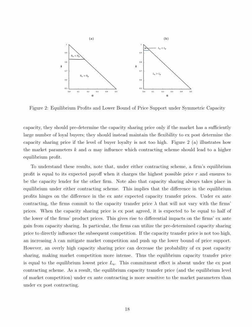
3.4 Ex Ante versus Ex Post Contracting

We now compare the ex ante and the ex post contracting schemes. The central question we address

is when the firms should contract over their capacity transfer price.

Proposition 5 When k converges to 1/2, Πa − Πp > 0. When k converges to 1− α, Πa − Πp > 0

if and only if α is greater than some threshold α′ ∈ (0, 1/2).

This proposition presents conditions under which the firms should adopt one of the contract-

ing schemes over the other. When the firms’ endowed capacity is sufficiently small, they should

unambiguously choose the ex ante contracting scheme and commit to their capacity transfer price

before they compete in the product market. However, when the firms have sufficient supply of

17

0.0 0.1 0.2 0.3 0.4 0.5

0.9

0.8

0.7

0.6

1

0.5

α

k

Π Π

Π Π

( a )

0.0 0.1 0.2 0.3 0.4 0.5

0.9

0.8

0.7

0.6

1

0.5

α

k

( b )

Figure 2: Equilibrium Profits and Lower Bound of Price Support under Symmetric Capacity

capacity, they should pre-determine the capacity sharing price only if the market has a sufficiently

large number of loyal buyers; they should instead maintain the flexibility to ex post determine the

capacity sharing price if the level of buyer loyalty is not too high. Figure 2 (a) illustrates how

the market parameters k and α may influence which contracting scheme should lead to a higher

equilibrium profit.

To understand these results, note that, under either contracting scheme, a firm’s equilibrium

profit is equal to its expected payoff when it charges the highest possible price r and ensures to

be the capacity lender for the other firm. Note also that capacity sharing always takes place in

equilibrium under either contracting scheme. This implies that the difference in the equilibrium

profits hinges on the difference in the ex ante expected capacity transfer prices. Under ex ante

contracting, the firms commit to the capacity transfer price λ that will not vary with the firms’

prices. When the capacity sharing price is ex post agreed, it is expected to be equal to half of

the lower of the firms’ product prices. This gives rise to differential impacts on the firms’ ex ante

gain from capacity sharing. In particular, the firms can utilize the pre-determined capacity sharing

price to directly influence the subsequent competition. If the capacity transfer price is not too high,

an increasing λ can mitigate market competition and push up the lower bound of price support.

However, an overly high capacity sharing price can decrease the probability of ex post capacity

sharing, making market competition more intense. Thus the equilibrium capacity transfer price

is equal to the equilibrium lowest price La. This commitment effect is absent under the ex post

contracting scheme. As a result, the equilibrium capacity transfer price (and the equilibrium level

of market competition) under ex ante contracting is more sensitive to the market parameters than

under ex post contracting.

18

As demonstrated in Figure 2 (b), the lower bound of price support under ex ante contracting

is higher than that under ex post contracting when k is sufficiently low or when α is sufficiently

high. This is driven by the commitment effect discussed above. When k converges to 1/2 and

the product market is least competitive, a high capacity transfer price can be committed without

worrying much about reducing the chance of capacity sharing. The firms’ incentive to cut product

prices can then be mitigated more under the ex ante contracting scheme, i.e., La > Lp. In contrast,

when k converges to 1−α and the market becomes sufficiently competitive, the firms have to commit

to a sufficiently low capacity sharing price to maximize the probability of capacity sharing. The

equilibrium lower bound of price support can then be lower than that under ex post contracting,

unless the size of loyal buyers is large enough such that the market is not overly competitive.

Therefore, the firms are less aggressive in price competition under ex ante contracting than

under ex post contracting if the market is sufficiently uncompetitive, but the reverse would be true

in a sufficiently competitive market. This explains why the firms’ equilibrium profit under ex ante

contracting is higher than that under ex post contracting when the market is not very competitive

(i.e., k is sufficiently low or α is high enough).

As shown in Figure 2, there exist scenarios under which, even though the lower bound of

price support is higher under ex ante contracting, the equilibrium profit under ex post contracting

is higher. This is due to the flexibility in modifying the capacity transfer price under ex post

contracting. In contrast to the ex ante contracting scheme, the capacity transfer price under ex post

contracting can be adjusted upward if the firms turn out to charge high product prices. Therefore,

if ex ante contracting does not sufficiently soften competition (i.e., La is not too high relative to

Lp), the ex ante expected capacity transfer price can actually be higher under ex post contracting.

This is a favorable force for the equilibrium profit under the ex post contracting scheme.

4 Asymmetric Capacity

In this section we investigate the alternative scenario of asymmetric capacity, in which firm A is

not constrained in supplying its potential demand (i.e., a total size of 1 − α), whereas firm B has

limited capacity k ∈ (1/2, 1−α). All other assumptions under symmetric capacity are maintained.

As a result, the transfer of capacity can only be unilateral from firm A to firm B, and capacity

sharing is relevant only when firm B is the firm with relatively lower price than firm A.

19

4.1 No Capacity Sharing

The equilibrium structure is similar to that for the asymmetric setup considered in Narasimhan

(1988). In particular, the only equilibrium is in mixed strategy, and the equilibrium price support

for both firms is between r and some lower bound L. Nevertheless, there is a mass point at r for

the firm that is less price aggressive relative to the competitor.

To determine the equilibrium price support, let us consider the firms’ incentives to cut price to

compete for the switchers. Firm A can guarantee a profit of r(α + s) by setting its price equal to

r, whereas its maximum demand, by charging a lower price than firm B, is 1 − α. Thus firm A

will never set a price lower than r(α+s)1−α . In contrast, firm B’s ensured profit is equal to rα, and the

maximum sales it can seize can only be k units. This means that it is dominated for firm B to

charge a price lower than rα/k. Therefore, the equilibrium lower bound of price support for both

firms is Lo = maxr(α+s)

1−α , rα/k

, because in equilibrium no firm wants to charge a price strictly

lower than the competitor with probability one.

The firms’ equilibrium payoffs are given by ΠAo = Lo(1 − α) and ΠBo = Lok. The firm that is

more aggressive in price cut can earn an equilibrium profit that is higher than what can be gained

from its “guaranteed demand” by charging the highest possible price r (i.e., α + s for firm A and

α for firm B, respectively).

Lemma 1 In the benchmark case without capacity sharing under asymmetric capacity: (i) When

1/2 < k < minα(1−α)1−2α

, 1− α

, Lo = rα/k, ΠAo = rα(1 − α)/k > r(α + s) and ΠBo = rα; (ii)

When max

1/2, α(1−α)1−2α

< k < 1− α, Lo = r(α+s)

1−α , ΠAo = r(α + s) and ΠBo = r(α+s)k1−α > rα.

When firm B’s capacity is sufficiently small (or α is high enough), its incentive for price cut

would be lower than that of firm A. The equilibrium lower bound of price support is then given

by Lo = rα/k, and firm A earns an equilibrium profit higher than its guaranteed payoff. However,

when firm B has enough capacity (or α is low enough), it would become more aggressive than firm

A. This would lead to Lo = r(α+s)1−α , and firm B’s equilibrium payoff is higher than that from its

ensured demand. In other words, the pricing incentive of the less aggressive firm determines the

firms’ common price support, whereas the more aggressive firm enjoys a pricing advantage over the

rival. Intuitively, the equilibrium lower bound of price support increases in α and decreases in k.

Similar to the symmetric capacity scenario, firm A’s equilibrium profit ΠAo first decreases and

then increases in α, and decreases in k. In contrast, firm B’s equilibrium profit ΠBo unambiguously

increases in α, but can first increase and then decrease in k. Therefore, an increase in α has

qualitatively different impacts on the firms’ equilibrium profits here. This is because, as in the

20

case of symmetric capacity, firm A can enjoy the demand from the rationed switchers when the

rival is capacity constrained. This demand switching effect does not apply to firm B because firm

A does not have the problem of capacity constraint. This asymmetry is also the driving force for

the differential impacts of k on the firms’ equilibrium profits. From firm A’s perspective, a higher

k implies that the competitor not only becomes more price aggressive but also has less rationed

switchers. However, although an increase in firm B’s capacity k makes firm A more aggressive in

price competition by reducing the size of the rationed switchers, it can improve firm B’s ability to

satisfy its demand. The second effect is particularly relevant when firm B is more aggressive than

firm A and hence is more likely to win the demand of the switchers. These two effects can interact

with each other to yield the “inverted-U” impact on firm B’s equilibrium profit.

4.2 Ex Ante Contracting

We start with solving for the firms’ equilibrium pricing strategies in the second stage, conditional on

the capacity transfer price λ. This would allow us to derive the firms’ subgame-perfect equilibrium

profits, ΠA(λ) and ΠB(λ). Similar to the scenario of symmetric capacity, there are two possible

cases, depending on whether the capacity transfer price, λ, is lower or higher than the equilibrium

lower bound of price support L. Consider first the case L ≥ λ. The firms’ expected profits of setting

price p are, respectively,

πA(p) =∫ p

L[p(α + s) + λw] dFB(pB) +

∫ r

pp(1− α)dFB(pB), (6)

πB(p) =∫ p

LpαdFA(pA) +

∫ r

p[pk + (p− λ)w] dFA(pA). (7)

Firm A shares its capacity with firm B only when firm A charges a higher product price than firm

B does. The equilibrium can be solved by applying the following conditions: π′i(p) = 0, Fi(L) = 0,

i = A,B, and FA(r) = 1 > FB(r) or FB(r) = 1 > FA(r).

Consider then the alternative case L ≤ λ. A firm’s expected profit depends on whether its

charged price is lower or higher than the capacity transfer price. If the product price is p ≤ λ,

πA(p) =∫ p

Lp(α + s)dFB1(pB) +

∫ λ

pp(1− α)dFB1(pB) +

∫ r

λp(1− α)dFB2(pB), (8)

πB(p) =∫ p

LpαdFA1(pA) +

∫ λ

ppkdFA1(pA) +

∫ r

λpkdFA2(pA). (9)

If the product price is p ≥ λ,

21

πA(p) =∫ λ

Lp(α + s)dFB1(pB) +

∫ p

λ[p(α + s) + λw] dFB2(pB) +

∫ r

pp(1− α)dFB2(pB), (10)

πB(p) =∫ λ

LpαdFA1(pA) +

∫ p

λpαdFA2(pA) +

∫ r

p[pk + (p− λ)w] dFA2(pA). (11)

Similarly, we can solve for the equilibrium by applying the following conditions: π′i(p) = 0,

Fi1(L) = 0, Fi1(λ) = Fi2(λ), i = A,B, and FA2(r) = 1 > FB2(r) or FB2(r) = 1 > FA2(r).

Proposition 6 In the second-stage price competition under the ex ante contracting scheme and

under asymmetric capacity: (i) If λ ≤ r(α+s)1−α−w , the lower bound of the equilibrium price support

is La = r(α+s)+λw1−α , firm A’s equilibrium profit ΠA(λ) = La(1 − α) increases in λ, and firm B’s

equilibrium profit ΠB(λ) = Lak + (La − λ)w decreases in λ; (ii) If λ ≥ r(α+s)1−α−w , the lower bound of

the equilibrium price support is La = max

(α+s)[r(1−2α−s)−λw](1−α)(k−α)

, rα/k, r(α+s)1−α

, firm A’s equilibrium

profit ΠA(λ) = La(1 − α) decreases (weakly) in λ, and firm B’s equilibrium profit ΠB(λ) = Lak

decreases (weakly) in λ.

Similar to the symmetric capacity scenario, firm A’s equilibrium profit first increases and then

decreases in the capacity transfer price. This is also driven by a higher λ increasing the revenue,

but decreasing the likelihood, of capacity lending. In comparison, firm B, the capacity borrower, is

always hurt by an increasing capacity transfer price.

Recall that, under symmetric capacity, capacity sharing always softens market competition and

improves the firms’ profitability for any capacity transfer price. Does this intuitive result still hold

under asymmetric capacity?

Proposition 7 Under asymmetric capacity, firm A’s equilibrium profit under the ex ante contract-

ing scheme (i.e., ΠA(λ)) is lower than that without capacity sharing (i.e., ΠAo), if and only if

1/2 < k < minα(1−α)1−2α

, 1− α

and λ is sufficiently low.

Interestingly, this proposition suggests that capacity sharing under the ex ante contracting

scheme can be harmful to firm A’s profitability. There are two conditions for this surprising result

to arise. The first condition is that firm B’s capacity is sufficiently small (or the size of loyal buyers is

large). This ensures that, as shown in Lemma 1, without capacity sharing firm B is less aggressive in

price competition than firm A is and thus firm A can seize the demand from the switchers without

overly cutting its price. This relative pricing advantage implies that firm A can make a higher

profit than its guaranteed payoff r(α + s). However, capacity sharing increases firm A’s expected

22

payoff of maintaining high prices without enhancing its payoff of undercutting the competitor. In

contrast, price cut becomes relatively more attractive to firm B because the increasing demand can

be satisfied by borrowed capacity. Firm B would become more aggressive than firm A, and firm A

would then lose its relative pricing advantage it enjoys in the case without capacity sharing. As

a result, if this strategic effect is strong enough while the main effect of increasing the capacity

transfer price is limited (i.e., λ is sufficiently low), capacity sharing can intensify competition and

firm A would be worse off under the ex ante contracting scheme.

This surprising result stands in contrast to that under symmetric capacity. Both firms are

always the same aggressive in price competition in the symmetric scenario, i.e., no firm has a higher

incentive for price cut than the competitor does. Similarly, either firm can be the capacity lender

or the borrower in the symmetric case, and capacity sharing does not change the symmetry in the

firms’ pricing aggressiveness. Therefore, capacity sharing can exert only the main effect of matching

excessive supply with unserved demand, and thus can unambiguously soften competition for both

firms. It is only when the firms are asymmetric in their incentives for price cut that capacity

sharing may exert the strategic influence of reversing the relative aggressiveness between the firms.

Nevertheless, note that firm B cannot be hurt by capacity sharing. Because capacity sharing is

unilateral and can arise only if firm B charges a lower product price than firm A does, it can make

the capacity lender less aggressive and the borrower more aggressive, but not vice versa. As a result,

firm B can gain, but cannot lose, its relative pricing advantage over firm A.

This result suggests that firms should be cautious in setting their capacity transfer price. This is

also a critical issue for scrutiny when the capacity transfer price is determined exogenously or by a

third party. For example, in some regulated industry (e.g., telecommunication), the infrastructure

sharing price between an incumbent with large capacity and an entrant with limited capacity is

determined by the government. Our analysis above shows that the high-capacity incumbent may

be hurt by capacity sharing arrangements if the capacity sharing price is too low.

We now determine the equilibrium capacity transfer price in the first stage of the game. When

firm A is to make the offer, it is desirable to increase the capacity transfer price while maximizing the

probability of capacity sharing. Note also that, for any λ ∈ (0, r), firm B is weakly better off than

in the case of no capacity sharing. This means that firm A will optimally set λ = r(α+s)1−α−w , which will

be accepted by firm B. It can be shown that firm A’s optimal offer increases in α and decreases in k.

Alternatively, when firm B gets the opportunity to make the proposal, it will offer the lowest possible

capacity transfer price at which firm A is indifferent between acceptance and rejection, because firm

B’s profit ΠB(λ) decreases in λ. As a result, if 1/2 < k < minα(1−α)1−2α

, 1− α

, firm B has to set

λ = r[α(1−α)−(α+s)k]wk

. However, if max

1/2, α(1−α)1−2α

< k < 1 − α, firm B will be able to set λ = 0.

In other words, the optimal offer for firm B can be represented as λ = maxr[α(1−α)−(α+s)k]

wk, 0

.

23

4.3 Ex Post Contracting

The firms may engage in capacity sharing if and only if firm B charges a lower product price than

firm A does. As a result, if pA ≤ pB, the firms’ profits are πA = pA(1 − α) and πB = pBα. If

pA ≥ pB, firm A will offer a capacity transfer price that is equal to λ = pB, whereas firm B will

propose λ = 0. In anticipation of this, the firms’ expected profits of setting price p in the first stage

are, respectively,

πA(p) =∫ p

L[p(α + s) + pBw/2] dFB(pB) +

∫ r

pp(1− α)dFB(pB), (12)

πB(p) =∫ p

LpαdFA(pA) +

∫ r

p(pk + pw/2)dFA(pA). (13)

Similarly, we can apply the following conditions to solve for the equilibrium: π′i(p) = 0, Fi(L) =

0, i = A,B, and FA(r) = 1 > FB(r) or FB(r) = 1 > FA(r).

Proposition 8 Under the ex post contracting scheme and under asymmetric capacity, the equilib-

rium lower bound of price support is Lp = max

r(α+s1−α

) 1−2α−s−w/21−2α−s , rα

k+w/2

, and the firms’ equilib-

rium profits are ΠAp = Lp(1− α) and ΠBp = Lp(k + w/2), respectively.

The two components in Lp reflect firm A’s and firm B’s incentive to undercut the competitor,

respectively. In comparison to the case without capacity sharing, firm A has a higher incentive to be

the higher-priced firm, and thus the lowest price it is willing to charge becomes higher. In contrast,

due to the gain from capacity sharing, now the payoff of charging a lower price than the rival is

higher for firm B. In other words, the ex post contracting scheme makes firm A less aggressive and

firm B more aggressive. Then what is the payoff implication of this differential change in the firms’

pricing aggressiveness?

Proposition 9 Under asymmetric capacity, firm A’s equilibrium profit under the ex post contract-

ing scheme, ΠAp, can be lower than that without capacity sharing, ΠAo.

Interestingly, this proposition shows that firm A’s equilibrium profit can actually be hurt by

capacity sharing under the ex post contracting scheme. That is, even though lending excessive

capacity to the competitor is ex post beneficial, it may reduce firm A’s ex ante profitability. In the

Appendix we present conditions for this counter-intuitive result to happen. As the proof implies,

one necessary condition is that firm A is more aggressive than firm B in the case without capacity

sharing and that the reverse is true under the ex post contracting scheme. It is only when the relative

24

0.0 0.1 0.2 0.3 0.4 0.5

0.9

0.8

0.7

0.6

1

0.5

α

k

Π ΠΠΠ

0.0 0.1 0.2 0.3 0.4 0.5

0.9

0.8

0.7

0.6

1

0.5

α

k

Π ΠΠΠ

( a ) ( b )

Figure 3: Comparison of Firm A’s Equilibrium Profits under Asymmetric Capacity

pricing aggressiveness between the firms can be reversed that price competition can be intensified.

Moreover, for the equilibrium lower bound of price support (and hence firm A’s equilibrium payoff)

to be lowered, it must be the case that firm B has a less compelling incentive for price cut in the case

without capacity sharing than firm A does under the ex post contracting scheme. This may arise in

the parameter range under which, as Figure 3 (a) demonstrates, α is sufficiently high. In contrast,

firm B always benefits from capacity sharing. Intuitively, this is because the reversal in the firms’

aggressiveness is only in one way but not the other. In other words, by becoming relatively more

aggressive in price cut, a firm may hurt the rival but cannot hurt itself.

This differential impact of capacity sharing on the firms’ pricing aggressiveness arises in the ex

ante contracting scheme as well. It is also the driving force there for the result in Proposition 7 that

capacity sharing can be harmful for firm A if the capacity transfer price is too low. However, when

the firms can ex ante determine the capacity transfer price, no firm will accept an offer that makes

it worse off than the outside option of no capacity sharing. This means that, under the equilibrium

capacity transfer price, the harmful impact of capacity sharing can be shunned (i.e., ΠAa > ΠAo).

Nevertheless, Proposition 9 suggests that, when the firms cannot commit to the capacity sharing

price, the firm with excessive capacity may be hurt.

4.4 Ex Ante Versus Ex Post Contracting

Figure 3 presents the comparison of firm A’s equilibrium profits. Recall that the ex ante contracting

scheme always leads to a higher equilibrium profit than that without capacity sharing, whereas firm

A may be worse off under ex post contracting than under no capacity sharing. Similar to the

symmetric capacity case, firm A’s preference for ex ante versus ex post contracting is determined

25

by the difference in the ex ante expected capacity transfer prices. This is because in equilibrium

capacity sharing always takes place under either contracting scheme. Similar forces also influence the

difference in the ex ante expected capacity transfer prices. In particular, firm A desires to commit to

the highest possible capacity transfer price that maximizes the chance of capacity sharing, whereas

the capacity transfer price under ex post contracting is set conditional on the product prices.

Therefore, firm A’s optimal capacity sharing price under ex ante contracting is more sensitive to

the market parameters than the expected capacity sharing price under ex post contracting. As a

result, similar to Figure 2 (a), firm A is more likely to prefer to ex ante determine the capacity

transfer price when the market is relatively less competitive (e.g., α is sufficiently high).

There are, however, some notable differences from the symmetric case. First, asymmetric ca-

pacity may change the firms’ preferences for the capacity transfer price under ex ante contracting

but not under ex post contracting. Note that, when the firms are symmetric, both of them can be

the capacity borrower as well as the lender. Because at the time of pre-competition contracting the

firms do not know yet which firm will be the borrower or the lender, they share the same preference

to maintain the committed capacity transfer price. This differs from the asymmetric case, in which

the role of the firms in capacity sharing is pre-determined and firm B can only be the capacity

borrower but can never be the lender. This means that, firm B prefers to minimize the capacity

sharing price as much as possible under the ex ante contracting scheme. Nevertheless, asymmetric

capacity does not make this difference under ex post contracting. At the time the firms determine

the capacity transfer price after the product prices are set, under either symmetric or asymmetric

capacity, they know which firm is the seller or the buyer of excessive capacity. In other words, it is

only under ex ante contracting, but not under ex post contracting, that asymmetric capacity can

modify the firms’ knowledge about their relative role in capacity sharing. This then constitutes a

negative force to drive down the expected capacity transfer price under ex ante contracting relative

to that under the ex post contracting scheme.

The second difference is that firm A has more capacity under the asymmetric capacity scenario.

In comparison to the symmetric case, a higher capacity makes firm A more aggressive in price

cut. This also increases firm B’s aggressiveness, because it can sell only to its loyal buyers (i.e., no

rationed switchers for firm A) if it charges a higher price than the rival. As a result, both firms

are more aggressive under asymmetric capacity. Nevertheless, the increasing competitiveness has

a stronger impact on ex ante contracting than on the ex post contracting scheme. This is, again,

because the equilibrium capacity transfer price and the lower bound of price support under ex ante

contracting are more responsive to changes in the competitiveness of the market.

Because of these two differences, firm A may have an increasing preference for the ex post

contracting scheme. This can explain why, as the comparison between Figure 2 (a) and Figure

26

3 (b) shows, the parameter range under which firm A prefers ex post contracting is wider in the

asymmetric case than under symmetric capacity. For example, when k converges to 1/2, ex ante

contracting is always preferred for any α in Figure 2 (a), but ex post contracting may lead to a

higher equilibrium payoff for small α in Figure 3 (b).

In contrast, firm B always earns a larger equilibrium profit under the ex post contracting scheme

than under the ex ante contracting scheme (i.e., ΠBp > ΠBa). This can be explained by the more

intense market competition under asymmetric capacity as well, which has a stronger impact on

ex ante contracting. This result also suggests that the firms may have conflicting preferences for

the timing of contracting over the capacity transfer price. Even though the capacity lender may

prefer to pre-determine the capacity transfer price, the borrower may desire to postpone it until the

market competition is cleared. The competing firms would need to be more cautious in aligning

their interests about when they should engage in the determination of the capacity sharing price.

5 Concluding Remarks

5.1 Welfare Analysis

Collaborations among competitors, especially those that engage in agreements, are standard cases

for Antitrust investigation. The general guideline is to gauge competitive collaborations under the

rule of reason to determine the competitive and welfare implications. Therefore, a welfare analysis

of competitive capacity sharing is useful to address legal issues that may potentially arise.

Our focus in this research is on the efficiency-improving role of capacity sharing. When capacity

can be shared between competing firms, industry resources can be more efficiently allocated by

matching excessive supply with unmet demand. In particular, stockout may lead some loyal buyers

to be rationed and to leave the market without purchase, which would not arise if capacity sharing

is feasible. As a result, in our setup capacity sharing is always socially beneficial. For example, in

the symmetric capacity scenario, capacity sharing can increase social welfare from r(1− w) to r.

However, capacity sharing may not always increase buyer surplus. This is because capacity

sharing may mitigate price competition and thus increase firm profitability. Consider first the

symmetric capacity scenario. Recall that, without capacity sharing, each firm’s equilibrium profit

is r(α + s). Under the ex ante contracting scheme, this is increased to r(α + s) + λ∗w, resulting

in a change in buyer surplus by rw − 2λ∗w, where λ∗ = r(α+s)k−w . It can be readily verified that

buyer surplus is improved under the ex ante contracting scheme if and only if the firms’ endowed

capacity k is sufficiently high. Intuitively, as shown in Proposition 3, if k is low enough and hence

27

the market is not very competitive, the firms would be able to commit to a sufficiently high capacity

transfer price λ∗. The firms’ gain from capacity sharing would then exceed that of social welfare,

thus leading to a lower buyer surplus. In contrast, under the ex post contracting scheme, even if

k is very low, the expected capacity sharing price would not be overly high. We can numerically

verify that, in this case buyer surplus is always greater than that without capacity sharing.

The impact of capacity sharing on buyer surplus is less unambiguous under the asymmetric ca-

pacity scenario. On one hand, the improvement in social welfare is lower than that under symmetric

capacity. This is because now only the loyal buyers of firm B, but not those of firm A, may be

rationed by stockout. On the other hand, as shown in Propositions 7 and 9, capacity sharing be-

tween asymmetric firms may intensify price competition and hurt the profitability of the firm with

excessive capacity (i.e., firm A). Nevertheless, we can perform numerical analysis to show that,

under either contracting scheme, capacity sharing can improve buyer surplus unless the number of

loyal buyers is intermediate and the endowed capacity k is sufficiently low.

5.2 Summary and Future Research

Cooperation between competitors through capacity/inventory sharing is a prevalent phenomenon in

many retail and manufacturing settings. However, the interaction between competition and capacity

sharing is not well understood in the existing literature. In this paper we fill this gap by investigating

capacity trade between two firms that engage in price competition. We examine optimal strategies

and firm profitability of competitive capacity sharing under two alternative schemes, depending on

whether the firms agree over the price of capacity sharing before or after product price setting. Our

analysis yields some interesting results with substantial practical relevance.

When the firms have symmetric capacity, they share the same preference to commit to a capacity

sharing price that is high enough while maximizing the likelihood of sharing. This means that the

optimal capacity transfer price should take into account the influence on subsequent competition,

and be equal to the lowest possible product price the firms anticipate to charge in equilibrium. We

confirm that capacity sharing can indeed soften competition and lead to higher equilibrium profit

under either contracting scheme. We also find that ex ante contracting leads to equilibrium outcomes

that are more responsive to changes in market parameters, and thus tends to be more appealing

than ex post contracting in less competitive markets (e.g., less capacity or higher buyer loyalty).

Nevertheless, both the optimal sharing price and the equilibrium profit can be non-monotonically

influenced by the number of loyal buyers.

Our analysis reveals that these insights on competitive capacity sharing can be altered by asym-

metric capacity. It is not surprising that firms with different capacity may have differential incentives

28

about what capacity sharing price to commit. However, despite the gain from improving capacity

efficiency, capacity sharing can counter-intuitively intensify equilibrium competition and hurt the

profitability of the firm without capacity constraint. This surprising result arises when capacity

sharing reverses the relative pricing aggressiveness between the firms and makes the less competitive

firm under no capacity sharing more competitive.

An important feature of our current model is that a firm’s role in capacity sharing is endogenously

determined by price competition. That is, depending on the relative prices between the competitors,

a firm may become either the capacity borrower or the capacity lender. Nevertheless, the prospect

of capacity sharing is certain in the sense that, conditional on the outcome of price competition, it

is common knowledge which firm will be in stockout and which firm has excess capacity to lend.

If demand is stochastic instead, there would exist (extra) uncertainty about the firms’ roles in

capacity sharing. That is, a firm charging relatively lower product price may not necessarily be

short of capacity, and conversely, a firm with relatively higher price may not have excess capacity.

Considering this extension can definitely make the model more realistic and expand the scope of

research issues, while we believe that the main insights derived in current research would continue

to hold.

We consider exogenous search behavior for the switchers in the case of stockout. That is, we

assume that once the switchers are rationed and the inventory is not furnished immediately, they will

turn to the competitor to make the purchase. This would be a reasonable assumption if the rationed

switchers are unaware or ignorant of the prospect of capacity sharing between the competing firms.

Nevertheless, in scenarios when capacity sharing between competitors is prevalent, rationed buyers

may strategically decide whether and when to search for alternative firms. This endogenous search

behavior may then influence the firms’ optimal timing for the sharing of capacity. We leave this

interesting but challenging problem for future research.

There are several extensions that can be investigated in future research. One interesting issue

is regarding the role of firm differentiation in strategic capacity sharing. It is assumed in the

current paper that the product transferred from the competitor has the same value as own product.

New insights may arise if this assumption is relaxed and the firms are horizontally or vertically

differentiated such that the bought capacity involves differential utility for the buyers.

Future research can investigate other aspects of capacity sharing that have not been addressed in

the current paper. For example, firms can negotiate and commit to not only the price, but also the

volume, of capacity sharing. It may also be interesting to consider non-linear contracts such as two-

part tariff. Another interesting extension is to endogenize the timing of bargaining (Guo and Iyer

2013). For example, the outside option of breakdown for ex ante contracting is not the no-sharing

29

case, but the ex post contracting case. Finally, future studies can consider virtual capacity sharing

without the actual transfer of property rights. That is, firms can pool their capacity together that

can be used to satisfy any participating firm’s demand. This is particularly relevant for service

industries (e.g., airlines) in which orders can be taken through advance reservation.

30

Appendix

Proof of Proposition 2: (i) Consider the first possible case L ≥ λ. The firms’ expected profit of

setting the price p is given by

π(p) =∫ pL [p(α + s) + λw] f(p′)dp′ +

∫ rp [pk + (p− λ)w] f(p′)dp′

= pF (p)(α + s− w − k) + 2λwF (p) + p(w + k)− λw.

Taking the first order derivative with respect to p yields π′(p) = [F (p) + pf(p)] (α+s−w−k)+

2λwf(p) + w + k = 0. Solving this differential equation by using the boundary condition F (r) = 1

leads to F (p) = r(α+s)+2λw−(w+k)p2λw+(α+s−w−k)p

.

Furthermore, we can impose the condition F (L) = 0 to solve for the lower bound of price support

L = r(α+s)+2λww+k

. It follows that the condition L ≥ λ is equivalent to λ ≤ r(α+s)k−w .

The firms’ equilibrium profit in this case is Π(λ) = r(α + s) + λw. It is straightforward thatdΠ(λ)dλ

= w > 0. Thus, Π(λ) increases in λ for λ ≤ r(α+s)k−w .

(ii) Consider then the alternative case L ≤ λ. The firms’ profit by setting the price p ≥ λ is:

π(p) =∫ λL p(α + s)f1(p′)dp′ +

∫ pλ [p(α + s) + λw] f2(p′)dp′ +

∫ rp [pk + (p− λ)w] f2(p′)dp′

= pF2(p)(α + s− w − k) + 2λwF2(p) + p(w + k)− [1 + F1(λ)]λw.

Taking the first order derivative with respect to p yields π′(p) = [F2(p) + pf2(p)] (α + s − w −k) + 2λwf2(p) + w + k = 0. Solving this differential equation by using the boundary condition

F2(r) = 1 leads to F2(p) = r(α+s)+2λw−(w+k)p2λw+(α+s−w−k)p

.

The firms’ profit by setting the price p ≤ λ is:

π(p) =∫ pL p(α + s)f1(p′)dp′ +

∫ λp pkf1(p′)dp′ +

∫ rλ pkf2(p′)dp′

= pF1(p)(α + s− k) + pk.

Taking the first order derivative of π(p) with respect to p leads to [F1(p) + pf1(p)] (α+s−k)+k =

0. Solving this differential equation by using the boundary condition F1(λ) = F2(λ) leads to

F1(p) = kk−α−s + (α+s)[r(α+s−k)+λw]

(k−α−s)(k−α−s−w)p.

We impose the condition F1(L) = 0 to solve for the lower bound of price support L =(α+s)[r(α+s−k)+λw]

k(α+s+w−k). It follows that the condition L ≤ λ is equivalent to λ ≥ r(α+s)

k−w .

The firms’ equilibrium profit in this case is Π(λ) = Lk = r(α + s) + (α+s)(r−λ)wk−α−s−w . Therefore, we

have dΠ(λ)dλ

= (α+s)wα+s+w−k < 0. Thus, Π(λ) decreases in λ for λ ≥ r(α+s)

k−w .

31

Proof of Proposition 3: Note that λ∗ = r(α+s)k−w , where s = (1 − 2α)

(1− k

1−α

)and w =

α(1− k

1−α

). Therefore, dλ∗

dα=

r(2k−1)[k−(1−α)2](k−α+α2)2

. Thus, λ∗ decreases in α for α < 1 −√k, and

increases in α for α > 1−√k. Moreover, dλ∗

dk< 0, because both s and w decrease in k.

Note that Πa = Lak = λ∗k. It follows that dΠadα

= k dλ∗

dα. Therefore, Πa first decreases in α for

α < 1−√k and then increases in α for α > 1−

√k. Note also that Πa ≡ Π(λ∗) = r(α+s)+ r(α+s)

k−w w =r(α+s)kk−w . Therefore, we have dΠa

dk= r−(1−2α)k2+2α(1−α)(1−2α)k−α(1−α)3

(k−α+α2)2. Let Ω = −(1− 2α)k2 + 2α(1−

α)(1 − 2α)k − α(1 − α)3. It can be readily verified that Ω is a concave function of k, with the

maximum value achieved at k = α(1− α). Moreover, Ω|k=α(1−α) = −α(1− α)2(1− 2α + 2α2) < 0.

Therefore, dΠadk

< 0 for all k.

Proof of Proposition 4: Note that Πa−Πo = r(α+s)k−w w. We have d(Πa−Πo)

dα=

[(1−α)2−k]rΓ(1−α)2[k−α(1−α)]2

, where

Γ = (−2α2 + 4α− 1)k2 + (3α2 − 4α+ 1)k+ α2(1− α)2. Note that Γ|k=1/2 = (1− 2α+ 2α2)2/4 > 0

and Γ|k=1−α = α(1− α)3 > 0. The derivative of Γ with respect to k, evaluated at k = 1/2, is equal

to α2 > 0. It follows that Γ > 0 for all k ∈ (1/2, 1 − α), because the second order derivative of Γ

with respective to k is independent of k. Therefore, d(Πa−Πo)dα

> 0 for α < 1−√k, and d(Πa−Πo)

dα< 0

for α > 1−√k. Moreover, d(Πa−Πo)

dk< 0, because both s and w decrease in k.

Proof of Proposition 5: To compare Πa with Πp, we just need to compare Ia = kk−w with

Ip =(

α+sk+w/2

) w/2α+s−w/2−k , where s = (1− 2α)(1− k/(1− α)) and w = α(1− k/(1− α)).

Evaluating Ia− Ip at k = 1/2 leads to (Ia − Ip) |k=1/2 = 1−α1−2α(1−α)

−(

2−4α+4α2

2−α−2α2

)− 13 , which can be

shown to be strictly positive for α ∈ (0, 1/2). By the continuity of Ia − Ip in k, we then prove that

Ia − Ip > 0 when k is sufficiently close to 1/2.

We have ∂(Ia−Ip)∂k|k=1−α = α

2(1−2α)(1−α)2[4α− 2− (1− α) log(α/(1− α))]. It can be readily veri-

fied that 4α− 2− (1−α) log(α/(1−α)) is convex, its first order derivative evaluated at α = 1/2 is

positive, and its value evaluated at α = 0 is positive and evaluated at α = 1/2 is zero. Therefore,

there must exist an α′ ∈ (0, 1/2) such that ∂(Ia−Ip)∂k|k=1−α > 0 for 0 < α < α′ and ∂(Ia−Ip)

∂k|k=1−α < 0

for α′ < α < 1/2. It then follows from (Ia − Ip) |k=1−α = 0 that, for k sufficiently close to 1 − α,

Ia − Ip < 0 if 0 < α < α′, and Ia − Ip > 0 if α′ < α < 1/2.

Proof of Lemma 1: Following Narasimhan (1988), the equilibrium lower bound of price support

is given by Lo = maxr(α+s)

1−α , rα/k

. Note that r(α+s)1−α > rα/k if and only if ∆(k) = −1−2α

1−α k2 +

(1− α)k − α(1− α) > 0. ∆(k) is concave in k. Solving ∆(k) = 0 leads to two solutions k1 = 1− αand k2 = α(1−α)

1−2α. Therefore, ∆(k) < 0 if and only if 1/2 < k < min

α(1−α)1−2α

, 1− α

. In this case we

32

have Lo = rα/k, and the firms’ equilibrium profits are ΠAo = Lo(1− α) = rα(1− α)/k > r(α + s)

and ΠBo = Lok = rα. In addition, ∆(k) > 0 if and only if max

1/2, α(1−α)1−2α

< k < 1− α, leading

to Lo = r(α+s)1−α , and the firms’ equilibrium profits ΠAo = Lo(1 − α) = r(α + s) and ΠBo = Lok =

r(α+s)k1−α > rα.

Note that α(1−α)1−2α

< 1/2 if and only if α < 1−√

2/2, and α(1−α)1−2α

< 1− α if and only if α < 1/3.

Thus 1/2 < α(1−α)1−2α

< 1− α if and only if α ∈(1−√

2/2, 1/3).

Proof of Proposition 6: (i) Consider the first possible case L ≥ λ. The firms’ expected profits

of setting the price p are given by

πA(p) =∫ pL [p(α + s) + λw] dFB(pB) +

∫ rp p(1− α)dFB(pB)

= pFB(p)(2α + s− 1) + λwFB(p) + p(1− α),

πB(p) =∫ pL pαdFA(pA) +

∫ rp [pk + (p− λ)w] dFA(pA)

= pFA(p)(α− w − k) + λwFA(p) + pk + (p− λ)w.

Setting FA(L) = FB(L) = 0 leads to πA(L) = L(1−α) and πB(L) = Lk+(L−λ)w. Substituting

into πi(p) = πi(L), i = A,B, yields FB(p) = (p−L)(1−α)p(1−2α−s)−λw and FA(p) = (p−L)(w+k)

p(w+k−α)−λw , respectively.

As a result, FA(r) = 1 leads to L = rα+λww+k

, and FB(r) = 1 leads to L = r(α+s)+λw1−α .

Suppose FA(r) = 1. Then L = rα+λww+k

≥ λ is equivalent to λ ≤ rα/k, and FB(r) < 1 is equivalent

to λ > r(1−2α)kα(1−α−k)

. But because rα/k < r(1−2α)kα(1−α−k)

, FA(r) = 1 is impossible.

Therefore, we must have FB(r) = 1 > FA(r) in equilibrium. This implies the equilibrium lower

bound of price support is La = r(α+s)+λw1−α . The condition L ≥ λ leads to λ ≤ r(α+s)

1−α−w , which can also

guarantee that FA(r) < 1 (i.e., λ < r(1−2α)kα(1−α−k)

). The firms’ equilibrium profits are ΠA(λ) = La(1−α)

and ΠB(λ) = Lak + (La − λ)w, respectively. It is straightforward that dΠA(λ)dλ

> 0 and dΠB(λ)dλ

< 0.

(ii) Consider then the alternative case L ≤ λ. If the price is p ≤ λ, the firms’ expected profits

areπA(p) =

∫ pL p(α + s)dFB1(pB) +

∫ λp p(1− α)dFB1(pB) +

∫ rλ p(1− α)dFB2(pB)

= pFB1(p)(2α + s− 1) + p(1− α),

πB(p) =∫ pL pαdFA1(pA) +

∫ λp pkdFA1(pA) +

∫ rλ pkdFA2(pA)

= pFA1(p)(α− k) + pk.

Setting FA1(L) = FB1(L) = 0 leads to πA(L) = L(1 − α) and πB(L) = Lk. Substituting into

πi(p) = πi(L), i = A,B, yields FB1(p) = (p−L)(1−α)p(1−2α−s) and FA1(p) = (p−L)k

p(k−α), respectively. As a result,

FA1(λ) = (λ−L)kλ(k−α)

and FB1(λ) = (λ−L)(1−α)λ(1−2α−s) .

33

If the price is p ≥ λ, the firms’ expected profits are

πA(p) =∫ λL p(α + s)dFB1(pB) +

∫ pλ [p(α + s) + λw] dFB2(pB) +

∫ rp p(1− α)dFB2(pB)

= pFB2(p)(2α + s− 1) + λw [FB2(p)− FB2(λ)] + p(1− α),

πB(p) =∫ λL pαdFA1(pA) +

∫ pλ pαdFA2(pA) +

∫ rp [pk + (p− λ)w] dFA2(pA)

= pFA2(p)(α− w − k) + λwFA2(p) + pk + (p− λ)w.

Evaluating the profit functions at p = λ leads to πA(λ) = λ(2α + s − 1)FB2(λ) + (1 − α)λ

and πB(λ) = λ(α − k)FA2(λ) + λk. Substituting into πi(p) = πi(λ), i = A,B, yields FB2(p) =(p−λ)(1−α)+λ(1−2α−s−w)FB2(λ)

p(1−2α−s)−λw and FA2(p) = (p−λ)(w+k)+λ(k−α)FA2(λ)p(w+k−α)−λw , respectively. These can be simpli-

fied, by substituting FB2(λ) = FB1(λ) = (λ−L)(1−α)λ(1−2α−s) and FA2(λ) = FA1(λ) = (λ−L)k

λ(k−α). As a result,

FA2(r) = 1 leads to L = rα/k, and FB2(r) = 1 leads to L = (α+s)[r(1−2α−s)−λw](1−α)(k−α)

.

Suppose FB2(r) = 1. Then L = (α+s)[r(1−2α−s)−λw](1−α)(k−α)

≤ λ is equivalent to λ ≥ r(α+s)1−α−w , and

FA2(r) < 1 is equivalent to λ < λ ≡ r[ks(1−s)−3αks+(1−k)α2−α3]k(α+s)w

. It can be shown that λ > r(α+s)1−α−w .

Suppose FA2(r) = 1. Then L = rα/k, and FB2(r) < 1 is equivalent to λ > λ. It can be shown that

λ > rα/k. Therefore, if r(α+s)1−α−w ≤ λ ≤ min

λ, r

, the equilibrium lower bound of price support is

La = (α+s)[r(1−2α−s)−λw](1−α)(k−α)

, which is decreasing in λ; if λ ≤ λ ≤ r, the equilibrium lower bound of price

support is La = rα/k.

Note that (α+s)[r(1−2α−s)−λw](1−α)(k−α)

≥ rα/k if and only if λ ≤ λ, λ ≤ r if and only if r(α+s)1−α ≤ rα/k,

and (α+s)[r(1−2α−s)−λw](1−α)(k−α)

converges to r(α+s)1−α when λ goes to r. This means that the equilibrium in the

case when λ ≥ r(α+s)1−α−w can be summarized as La = max

(α+s)[r(1−2α−s)−λw]

(1−α)(k−α), rα/k, r(α+s)

1−α

.

The firms’ equilibrium profits are ΠA(λ) = La(1 − α) and ΠB(λ) = Lak, respectively. It is

straightforward that dΠA(λ)dλ≤ 0 and dΠB(λ)

dλ≤ 0, because La decreases (weakly) in λ.

Proof of Proposition 7: Note from Lemma 1 that firm A’s equilibrium profit without capacity

sharing is ΠAo = rα(1 − α)/k > r(α + s) if and only if 1/2 < k < minα(1−α)1−2α

, 1− α

. From

Proposition 6, if λ ≤ r(α+s)1−α−w , firm A’s equilibrium profit under the ex ante contracting scheme is

ΠA(λ) = r(α + s) + λw, which is less than ΠAo = rα(1− α)/k if λ is sufficiently low.

It is also straightforward that, if λ ≥ r(α+s)1−α−w , we always have ΠA(λ) = La(1 − α) ≥ ΠAo =

Lo(1− α), because then La = max

(α+s)[r(1−2α−s)−λw](1−α)(k−α)

, rα/k, r(α+s)1−α

≥ Lo = max

r(α+s)

1−α , rα/k

.

34

Proof of Proposition 8: The firms’ expected profits of setting the price p are given by

πA(p) =∫ pL [p(α + s) + pBw/2] dFB(pB) +

∫ rp p(1− α)dFB(pB)

= pFB(p)(2α + s+ w/2− 1) + p(1− α)−∫ pL wFB(pB)/2dpB,

πB(p) =∫ pL pαdFA(pA) +

∫ rp (pk + pw/2)dFA(pA)

= pFA(p)(α− w/2− k) + p(k + w/2).

Taking the first order derivative with respect to p yields π′A(p) = FB(p)(2α+s−1)+pfB(p)(2α+

s+ w/2− 1) + 1− α = 0 and π′B(p) = FA(p)(α− w/2− k) + pfA(p)(α− w/2− k) + k + w/2 = 0,

respectively. Solving these differential equations, by using the boundary conditions FB(L) = 0 and

FA(L) = 0, respectively, leads to FB(p) = 1−α2α+s−1

( pL

)−1−2α−s

1−2α−s−w/2 + 1−α1−2α−s and FA(p) = (p−L)(k+w/2)

p(k+w/2−α).

As a result, FA(r) = 1 leads to L = rαk+w/2

, and FB(r) = 1 leads to L = r(α+s1−α

) 1−2α−s−w/21−2α−s .

Therefore, if r(α+s1−α

) 1−2α−s−w/21−2α−s > rα

k+w/2, in equilibrium we have FB(r) = 1 > FA(r) and

L = r(α+s1−α

) 1−2α−s−w/21−2α−s . If r

(α+s1−α

) 1−2α−s−w/21−2α−s < rα

k+w/2, in equilibrium we have FA(r) = 1 >

FB(r) and L = rαk+w/2

. In sum, the equilibrium lower bound of price support is given by Lp =

max

r(α+s1−α

) 1−2α−s−w/21−2α−s , rα

k+w/2

. The firms’ equilibrium profits follow immediately by substituting

FA(Lp) = FB(Lp) = 0 into the profit function Πip = πi(Lp), i = A,B, respectively.

Proof of Proposition 9: Note that ΠAp = Lp(1 − α) and ΠAo = Lo(1 − α). As a result,

ΠAp < ΠAo if and only if Lp = max

r(α+s1−α

) 1−2α−s−w/21−2α−s , rα

k+w/2

< Lo = max

r(α+s)

1−α , rα/k

. It is

straightforward that r(α+s1−α

) 1−2α−s−w/21−2α−s > r(α+s)

1−α and rαk+w/2

< rα/k. This means that Lp < Lo if and

only if ∆ =(α+s1−α

) 1−2α−s−w/21−2α−s − α/k < 0.

Evaluating ∆ at k = 1/2 leads to ∆|k=1/2 =(

1−2α+2α2

2(1−α)2

)1−α/2− 2α, which goes to 1/2 as α

converges to 0, and goes to 0 as α converges to 1/2. The derivative of ∆|k=1/2 with respect to α, as

α converges to 1/2, is positive. It can be verified that the second order derivative of ∆|k=1/2 with

respect to α is positive. Therefore, when k → 1/2, ∆ < 0 if and only if α is sufficiently high.

Alternatively, evaluating ∆ at k = 1 − α leads to ∆|k=1−α = 0. Taking the derivative of ∆

with respect to k and evaluating it at k = 1 − α leads to d∆dk|k=1−α =

α2 log( α1−α)−2+10α−12α2

2(1−2α)(1−α)2. The

denominator is always positive, and denote the numerator as N = α2 log(

α1−α

)− 2 + 10α − 12α2.

It can be readily verified that N |α=0 < 0, N |α=1/2 = 0, dNdα|α=1/2 = −1, and d2N

dα2 = 2 log(

α1−α

)−

(3−4α)(7−6α)(1−α)2

< 0. This proves that N > 0 if and only if α is above certain threshold. Therefore,

when k → 1− α, ∆ < 0 if and only if α is sufficiently high.

35

References

[1] Anupindi, R., Y. Bassok, E. Zemel. 2001. A general framework for the study of decentralized

distribution systems. Manufacturing and Service Operations Management, 3(4), 349-368.

[2] Apostolides, Z. 2014. Mazda officially opens Salamanca plant in Mexico. Automotive Logistics.

[3] Baake, P., J. Oechssler, C. Schenk. 1999. Explaining cross-supplies. Journal of Economics,

70(1), 37-60.

[4] Bidault, F., M. Schweinsberg. 1996. Fiat and Peugeot’s SevelNord Venture (A). IMD-3-0644.

[5] Brandenburger A.M., B.J. Nalebuff. 1996. Co-opetition. New York: Currency Doubleday.

[6] Brandenburger A., H. Stuart. 2007. Biform games. Management Science, 53(4), 537-549.

[7] Caldieraro, F. 2016. The role of brand image and product characteristics on firms’ entry and

OEM decisions. Management Science, Forthcoming.

[8] Chen, Y. 2010. Strategic outsourcing between rivals. Annals of Economics and Finance, 11(2),

301-311.

[9] Comez, N., K. E. Stecke, M. Cakanyildirim 2012. In-season transshipments among competitive

retailers. Manufacturing and Service Operations Management, 14(2), 290-300.

[10] Eisenstein, P.A. 2011. BMW, PSA Peugeot Citroen form battery car joint venture. The Detroit

Bureau.

[11] Granot, D., G. Sosic. 2003. A three-stage model for a decentralized distribution system of

retailers. Operations Research, 51(5), 771-784.

[12] Gurnani H., E. Murat, Y. Luo. 2007. Impact of product pricing and timing of investment

decisions on supply chain co-opetition. European Journal of Operational Research, 180(1), 228-

248.

[13] Guo, L., G. Iyer. 2013. Multilateral bargaining and downstream competition. Marketing Sci-

ence, 32(3), 411430.

[14] Honeywell. 2010. Honeywell and DuPont announce joint venture to manufacture new automo-

tive refrigerant. Honeywell Press Release.

[15] Hu, X., I. Duenyas, R. Kapuscinski. 2007. Existence of coordinating transshipment prices in a

two-location inventory model. Management Science, 53(8), 1289-1302.

36

[16] Hu, X., R. Caldentey, G. Vulcano. 2013. Revenue sharing in airline alliances. Management

Science, 59(5), 1177-1195.

[17] Huang, X., G. Sosic. 2011. Transshipment of inventories: Dual allocations vs. transshipment

prices. Manufacturing and Service Operations Management, 12(2), 299-318.

[18] Ihlwan, M. 2006. Samsung and Sony’s win-win LCD venture. BloombergBusinessweek.

[19] Jolly, D. 1997. Co-operation in a niche market: The case of fiat and PSA in multi purpose

vehicles. European Management Journal, 15(1), 35-44.

[20] Li, L., R.Q. Zhang. 2015. Cooperation through capacity sharing between competing forwarders.

Transportation Research Part E, 75, 115-131.

[21] Narasimhan, C. 1988. Competitive promotional strategies. Journal of Business, 61(4), 427-449.

[22] Reuters. 2012. UPDATE 1-Mazda to produce Toyota vehicles at its Mexico plant.

[23] Rudi, N., S. Kapur, D.F. Pyke. 2001. A two-location inventory model with transshipment and

local decision making. Management Science, 47(12), 1668-1680.

[24] Shulman, J.D. 2014. Product diversion to a direct competitor. Marketing Science, 33(3), 422-

436.

[25] Spiegel, Y. 1993. Horizontal subcontracting. RAND Journal of Economics, 24(4), 570-590.

[26] Tirole, J. 1988. The Theory of Industrial Organization. Cambridge: The MIT Press.

[27] Van Mieghem, J. A. 1999. Coordinating investment, production and subcontracting. Manage-

ment Science, 45(7), 954-971.

[28] Varian, H.R. 1980. A model of sales. American Economic Review, 70(4), 651-659.

[29] Wassmer, U., P. Dussauge, M. Planellas. 2010. How to manage alliances better than one at a

time. MIT Sloan Management Review, 51(3), 76-85.

[30] Wu, X., P. Kouvelis, H. Matsuo. 2013. Horizontal capacity coordination for risk management

and flexibility: Pay ex ante or commit a fraction of ex post demand? Manufacturing and

Service Operations Management, 15(3), 458-472.

[31] Wu, X., P. Kouvelis, H. Matsuo, H. Sano. 2014. Horizontal coordinating contracts in the

semiconductor industry. European Journal of Operational Research, 237(3), 887-897.

37

[32] Yu, Y., S. Benjaafar, Y. Gerchak. 2015. Capacity sharing and cost allocation among indepen-

dent firms with congestion. Production and Operations Management, 24(8), 1285-1310.

38