Capacity of Wireless Channels -...

4

Capacity of Wireless Channels

The growing demand for wireless communication makes it important to determine the ca-pacity limits of the underlying channels for these systems. These capacity limits dictatethe maximum data rates that can be transmitted over wireless channels with asymptoticallysmall error probability, assuming no constraints on delay or complexity of the encoder anddecoder. The mathematical theory of communication underlying channel capacity was pio-neered by Claude Shannon in the late 1940s. This theory is based on the notion of mutualinformation between the input and output of a channel [1; 2; 3]. In particular, Shannon de-fined channel capacity as the channel’s mutual information maximized over all possible inputdistributions. The significance of this mathematical construct was Shannon’s coding theo-rem and its converse. The coding theorem proved that a code did exist that could achieve adata rate close to capacity with negligible probability of error. The converse proved that anydata rate higher than capacity could not be achieved without an error probability boundedaway from zero. Shannon’s ideas were quite revolutionary at the time: the high data rateshe predicted for telephone channels, and his notion that coding could reduce error prob-ability without reducing data rate or causing bandwidth expansion. In time, sophisticatedmodulation and coding technology validated Shannon’s theory and so, on telephone linestoday, we achieve data rates very close to Shannon capacity with very low probability oferror. These sophisticated modulation and coding strategies are treated in Chapters 5 and 8,respectively.

In this chapter we examine the capacity of a single-user wireless channel where trans-mitter and/or receiver have a single antenna. The capacity of single-user systems wheretransmitter and receiver have multiple antennas is treated in Chapter 10 and that of multiusersystems in Chapter 14. We will discuss capacity for channels that are both time invariant andtime varying. We first look at the well-known formula for capacity of a time-invariant addi-tive white Gaussian noise (AWGN) channel and then consider capacity of time-varying flatfading channels. Unlike the AWGN case, here the capacity of a flat fading channel is notgiven by a single formula because capacity depends on what is known about the time-varyingchannel at the transmitter and/or receiver. Moreover, for different channel information as-sumptions there are different definitions of channel capacity, depending on whether capacitycharacterizes the maximum rate averaged over all fading states or the maximum constant ratethat can be maintained in all fading states (with or without some probability of outage).

99

100 CAPACITY OF WIRELESS CHANNELS

We will first consider flat fading channel capacity where only the fading distribution isknown at the transmitter and receiver. Capacity under this assumption is typically difficultto determine and is only known in a few special cases. Next we consider capacity when thechannel fade level is known at the receiver only (via receiver estimation) or when the chan-nel fade level is known at both the transmitter and the receiver (via receiver estimation andtransmitter feedback). We will see that the fading channel capacity with channel fade levelinformation at both the transmitter and receiver is achieved when the transmitter adapts itspower, data rate, and coding scheme to the channel variation. The optimal power alloca-tion in this case is a “water-filling” in time, where power and data rate are increased whenchannel conditions are favorable and decreased when channel conditions are not favorable.

We will also treat capacity of frequency-selective fading channels. For time-invariantfrequency-selective channels the capacity is known and is achieved with an optimal powerallocation that water-fills over frequency instead of time. The capacity of a time-varyingfrequency-selective fading channel is unknown in general. However, this channel can be ap-proximated as a set of independent parallel flat fading channels whose capacity is the sum ofcapacities on each channel with power optimally allocated among the channels. The capac-ity of such a channel is known and the capacity-achieving power allocation water-fills overboth time and frequency.

We will consider only discrete-time systems in this chapter. Most continuous-time sys-tems can be converted to discrete-time systems via sampling, and then the same capacity re-sults hold. However, care must be taken in choosing the appropriate sampling rate for thisconversion, since time variations in the channel may increase the sampling rate required topreserve channel capacity [4].

4.1 Capacity in AWGN

Consider a discrete-time AWGN channel with channel input /output relationship y[i] =x[i] + n[i], where x[i] is the channel input at time i, y[i] is the corresponding channel out-put, and n[i] is a white Gaussian noise random process. Assume a channel bandwidth B

and received signal power P. The received signal-to-noise ratio (SNR) – the power in x[i]divided by the power in n[i] – is constant and given by γ = P/N0B, where N0/2 is thepower spectral density (PSD) of the noise. The capacity of this channel is given by Shan-non’s well-known formula [1]:

C = B log2(1 + γ ), (4.1)

where the capacity units are bits per second (bps). Shannon’s coding theorem proves that acode exists that achieves data rates arbitrarily close to capacity with arbitrarily small probabil-ity of bit error. The converse theorem shows that any code with rate R > C has a probabilityof error bounded away from zero. The theorems are proved using the concept of mutual in-formation between the channel input and output. For a discrete memoryless time-invariantchannel with random input x and random output y, the channel’s mutual information is de-fined as

I(X; Y ) =∑

x∈X,y∈Yp(x, y) log

(p(x, y)

p(x)p(y)

), (4.2)

4.1 CAPACITY IN AWGN 101

where the sum is taken over all possible input and output pairs x ∈ X and y ∈ Y for X and Ythe discrete input and output alphabets. The log function is typically with respect to base 2,in which case the units of mutual information are bits per second. Mutual information canalso be written in terms of the entropy in the channel output y and conditional output y | x

as I(X; Y ) = H(Y ) − H(Y | X), where H(Y ) = −∑y∈Y p(y) log p(y) and H(Y | X) =

−∑x∈X,y∈Y p(x, y) log p(y | x). Shannon proved that channel capacity equals the mutual

information of the channel maximized over all possible input distributions:

C = maxp(x)

I(X; Y ) = maxp(x)

∑

x,y

p(x, y) log

(p(x, y)

p(x)p(y)

). (4.3)

For the AWGN channel, the sum in (4.3) becomes an integral over continuous alphabets andthe maximizing input distribution is Gaussian, which results in the channel capacity givenby (4.1). For channels with memory, mutual information and channel capacity are definedrelative to input and output sequences xn and y n. More details on channel capacity, mutualinformation, the coding theorem, and its converse can be found in [2; 5; 6].

The proofs of the coding theorem and its converse place no constraints on the complex-ity or delay of the communication system. Therefore, Shannon capacity is generally usedas an upper bound on the data rates that can be achieved under real system constraints. Atthe time that Shannon developed his theory of information, data rates over standard tele-phone lines were on the order of 100 bps. Thus, it was believed that Shannon capacity, whichpredicted speeds of roughly 30 kbps over the same telephone lines, was not a useful boundfor real systems. However, breakthroughs in hardware, modulation, and coding techniqueshave brought commercial modems of today very close to the speeds predicted by Shannonin the 1940s. In fact, modems can exceed this 30-kbps limit on some telephone channels,but that is because transmission lines today are of better quality than in Shannon’s day andthus have a higher received power than that used in his initial calculation. On AWGN ra-dio channels, turbo codes have come within a fraction of a decibel of the Shannon capacitylimit [7].

Wireless channels typically exhibit flat or frequency-selective fading. In the next twosections we consider capacity of flat fading and frequency-selective fading channels underdifferent assumptions regarding what is known about the channel.

EXAMPLE 4.1: Consider a wireless channel where power falloff with distance followsthe formula Pr(d ) = Pt(d0/d )3 for d0 = 10 m. Assume the channel has bandwidthB = 30 kHz and AWGN with noise PSD N0/2, where N0 = 10−9 W/Hz. For a trans-mit power of 1 W, find the capacity of this channel for a transmit–receive distance of100 m and 1 km.

Solution: The received SNR is γ = Pr(d )/N0B = .13/(10−9 ·30 ·103) = 33 = 15 dBfor d = 100 m and γ = .013/(10−9 · 30 ·103) = .033 = −15 dB for d = 1000 m. Thecorresponding capacities are C = B log2(1+ γ ) = 30000 log2(1+ 33) = 152.6 kbpsfor d = 100 m and C = 30000 log2(1 + .033) = 1.4 kbps for d = 1000 m. Note thesignificant decrease in capacity at greater distances due to the path-loss exponent of3, which greatly reduces received power as distance increases.


Figure 4.1: Flat fading channel and system model.

4.2 Capacity of Flat Fading Channels

4.2.1 Channel and System ModelWe assume a discrete-time channel with stationary and ergodic time-varying gain

√g[i], 0 ≤

g[i], and AWGN n[i], as shown in Figure 4.1. The channel power gain g[i] follows a givendistribution p(g); for example, with Rayleigh fading p(g) is exponential. We assume thatg[i] is independent of the channel input. The channel gain g[i] can change at each time i,either as an independent and identically distributed (i.i.d.) process or with some correlationover time. In a block fading channel, g[i] is constant over some blocklength T, after whichtime g[i] changes to a new independent value based on the distribution p(g). Let P denotethe average transmit signal power, N0/2 the noise PSD of n[i], and B the received signalbandwidth. The instantaneous received SNR is then γ [i] = Pg[i]/N0B, 0 ≤ γ [i] < ∞, andits expected value over all time is γ = Pg/N0B. Since P/N0B is a constant, the distributionof g[i] determines the distribution of γ [i] and vice versa.

The system model is also shown in Figure 4.1, where an input message w is sent fromthe transmitter to the receiver, which reconstructs an estimate w of the transmitted messagew from the received signal. The message is encoded into the codeword x, which is trans-mitted over the time-varying channel as x[i] at time i. The channel gain g[i], also called thechannel side information (CSI), changes during the transmission of the codeword.

The capacity of this channel depends on what is known about g[i] at the transmitter andreceiver. We will consider three different scenarios regarding this knowledge as follows.

1. Channel distribution information (CDI): The distribution of g[i] is known to the trans-mitter and receiver.

2. Receiver CSI: The value of g[i] is known to the receiver at time i, and both the transmit-ter and receiver know the distribution of g[i].

3. Transmitter and receiver CSI: The value of g[i] is known to the transmitter and receiverat time i, and both the transmitter and receiver know the distribution of g[i].

Transmitter and receiver CSI allow the transmitter to adapt both its power and rate to thechannel gain at time i, leading to the highest capacity of the three scenarios. Note that sincethe instantaneous SNR γ [i] is just g[i] multipled by the constant P/N0B, known CSI or CDIabout g[i] yields the same information about γ [i]. Capacity for time-varying channels underassumptions other than these three are discussed in [8; 9].

4.2.2 Channel Distribution Information KnownWe first consider the case where the channel gain distribution p(g) or, equivalently, the dis-tribution of SNR p(γ ) is known to the transmitter and receiver. For i.i.d. fading the capacity

4.2 CAPACITY OF FLAT FADING CHANNELS 103

is given by (4.3), but solving for the capacity-achieving input distribution (i.e., the distribu-tion achieving the maximum in that equation) can be quite complicated depending on thenature of the fading distribution. Moreover, fading correlation introduces channel memory,in which case the capacity-achieving input distribution is found by optimizing over inputblocks, and this makes finding the solution even more difficult. For these reasons, finding thecapacity-achieving input distribution and corresponding capacity of fading channels underCDI remains an open problem for almost all channel distributions.

The capacity-achieving input distribution and corresponding fading channel capacityunder CDI are known for two specific models of interest: i.i.d. Rayleigh fading channelsand finite-state Markov channels. In i.i.d. Rayleigh fading, the channel power gain is expo-nentially distributed and changes independently with each channel use. The optimal inputdistribution for this channel was shown in [10] to be discrete with a finite number of masspoints, one of which is located at zero. This optimal distribution and its corresponding capac-ity must be found numerically. The lack of closed-form solutions for capacity or the optimalinput distribution is somewhat surprising given that the fading follows the most commonfading distribution and has no correlation structure. For flat fading channels that are not nec-essarily Rayleigh or i.i.d., upper and lower bounds on capacity have been determined in [11],and these bounds are tight at high SNRs.

Approximating Rayleigh fading channels via FSMCs was discussed in Section 3.2.4. Thismodel approximates the fading correlation as a Markov process. Although the Markov natureof the fading dictates that the fading at a given time depends only on fading at the previoustime sample, it turns out that the receiver must decode all past channel outputs jointly withthe current output for optimal (i.e. capacity-achieving) decoding. This significantly compli-cates capacity analysis. The capacity of FSMCs has been derived for i.i.d. inputs in [12; 13]and for general inputs in [14]. Capacity of the FSMC depends on the limiting distribution ofthe channel conditioned on all past inputs and outputs, which can be computed recursively.As with the i.i.d. Rayleigh fading channel, the final result and complexity of the capacityanalysis are high for this relatively simple fading model. This shows the difficulty of obtain-ing the capacity and related design insights on channels when only CDI is available.

4.2.3 Channel Side Information at ReceiverWe now consider the case where the CSI g[i] is known to the receiver at time i. Equivalently,γ [i] is known to the receiver at time i. We also assume that both the transmitter and receiverknow the distribution of g[i]. In this case there are two channel capacity definitions that arerelevant to system design: Shannon capacity, also called ergodic capacity, and capacity withoutage. As for the AWGN channel, Shannon capacity defines the maximum data rate thatcan be sent over the channel with asymptotically small error probability. Note that for Shan-non capacity the rate transmitted over the channel is constant: the transmitter cannot adapt itstransmission strategy relative to the CSI. Thus, poor channel states typically reduce Shannoncapacity because the transmission strategy must incorporate the effect of these poor states.An alternate capacity definition for fading channels with receiver CSI is capacity with out-age. This is defined as the maximum rate that can be transmitted over a channel with anoutage probability corresponding to the probability that the transmission cannot be decodedwith negligible error probability. The basic premise of capacity with outage is that a highdata rate can be sent over the channel and decoded correctly except when the channel is in a


slow deep fade. By allowing the system to lose some data in the event of such deep fades,a higher data rate can be maintained than if all data must be received correctly regardless ofthe fading state, as is the case for Shannon capacity. The probability of outage characterizesthe probability of data loss or, equivalently, of deep fading.

SHANNON (ERGODIC) CAPACITY

Shannon capacity of a fading channel with receiver CSI for an average power constraint P

can be obtained from results in [15] as

C =∫ ∞

0B log2(1 + γ )p(γ ) dγ. (4.4)

Note that this formula is a probabilistic average: the capacity C is equal to Shannon capacityfor an AWGN channel with SNR γ, given by B log2(1 + γ ) and averaged over the distribu-tion of γ. That is why Shannon capacity is also called ergodic capacity. However, care mustbe taken in interpreting (4.4) as an average. In particular, it is incorrect to interpret (4.4) tomean that this average capacity is achieved by maintaining a capacity B log2(1 + γ ) whenthe instantaneous SNR is γ, for only the receiver knows the instantaneous SNR γ [i] andso the data rate transmitted over the channel is constant, regardless of γ. Note also that thecapacity-achieving code must be sufficiently long that a received codeword is affected by allpossible fading states. This can result in significant delay.

By Jensen’s inequality,

E[B log2(1 + γ )] =∫

B log2(1 + γ )p(γ ) dγ

≤ B log2(1 + E[γ ]) = B log2(1 + γ ), (4.5)

where γ is the average SNR on the channel. Thus we see that the Shannon capacity of a fad-ing channel with receiver CSI only is less than the Shannon capacity of an AWGN channelwith the same average SNR. In other words, fading reduces Shannon capacity when only thereceiver has CSI. Moreover, without transmitter CSI, the code design must incorporate thechannel correlation statistics, and the complexity of the maximum likelihood decoder will beproportional to the channel decorrelation time. In addition, if the receiver CSI is not perfect,capacity can be significantly decreased [16].

EXAMPLE 4.2: Consider a flat fading channel with i.i.d. channel gain√

g[i], whichcan take on three possible values:

√g1 = .05 with probability p1 = .1,

√g2 = .5

with probability p2 = .5, and√

g3 = 1 with probability p3 = .4. The transmit poweris 10 mW, the noise power spectral density N0/2 has N0 = 10−9 W/Hz, and the chan-nel bandwidth is 30 kHz. Assume the receiver has knowledge of the instantaneousvalue of g[i] but the transmitter does not. Find the Shannon capacity of this channeland compare with the capacity of an AWGN channel with the same average SNR.

Solution: The channel has three possible received SNRs: γ1 = Ptg1/N0B = .01 ·(.052)/(30000 · 10−9) = .8333 = −.79 dB, γ2 = Ptg2/N0B = .01 · (.52)/(30000 ·10−9) = 83.333 = 19.2 dB, and γ3 = Ptg3/N0B = .01/(30000 · 10−9) = 333.33 =25 dB. The probabilities associated with each of these SNR values are p(γ1) = .1,p(γ2) = .5, and p(γ3) = .4. Thus, the Shannon capacity is given by


C =∑

i

B log2(1 + γi)p(γi)

= 30000(.1log2(1.8333) + .5 log2(84.333) + .4 log2(334.33))

= 199.26 kbps.

The average SNR for this channel is γ = .1(.8333) + .5(83.33) + .4(333.33) =175.08 = 22.43 dB. The capacity of an AWGN channel with this SNR is C =B log2(1+175.08) = 223.8 kbps. Note that this rate is about 25 kbps larger than thatof the flat fading channel with receiver CSI and the same average SNR.

CAPACITY WITH OUTAGE

Capacity with outage applies to slowly varying channels, where the instantaneous SNR γ isconstant over a large number of transmissions (a transmission burst) and then changes to anew value based on the fading distribution. With this model, if the channel has received SNRγ during a burst then data can be sent over the channel at rate B log2(1 + γ ) with negligi-ble probability of error.1 Since the transmitter does not know the SNR value γ, it must fix atransmission rate independent of the instantaneous received SNR.

Capacity with outage allows bits sent over a given transmission burst to be decoded atthe end of the burst with some probability that these bits will be decoded incorrectly. Specif-ically, the transmitter fixes a minimum received SNR γmin and encodes for a data rate C =B log2(1+ γmin). The data is correctly received if the instantaneous received SNR is greaterthan or equal to γmin [17; 18]. If the received SNR is below γmin then the bits received overthat transmission burst cannot be decoded correctly with probability approaching 1, and thereceiver declares an outage. The probability of outage is thus Pout = p(γ < γmin). The aver-age rate correctly received over many transmission bursts is Cout = (1−Pout)B log2(1+γmin)

since data is only correctly received on 1 − Pout transmissions. The value of γmin is a de-sign parameter based on the acceptable outage probability. Capacity with outage is typicallycharacterized by a plot of capacity versus outage, as shown in Figure 4.2. In this figure weplot the normalized capacity C/B = log2(1+γmin) as a function of outage probability Pout =p(γ < γmin) for a Rayleigh fading channel (γ exponentially distributed) with γ = 20 dB.We see that capacity approaches zero for small outage probability, due to the requirement thatbits transmitted under severe fading must be decoded correctly, and increases dramatically asoutage probability increases. Note, however, that these high capacity values for large outageprobabilities have higher probability of incorrect data reception. The average rate correctlyreceived can be maximized by finding the γmin (or, equivalently, the Pout) that maximizes Cout.

EXAMPLE 4.3: Assume the same channel as in the previous example, with a band-width of 30 kHz and three possible received SNRs: γ1 = .8333 with p(γ1) = .1,γ2 = 83.33 with p(γ2) = .5, and γ3 = 333.33 with p(γ3) = .4. Find the capacityversus outage for this channel, and find the average rate correctly received for outageprobabilities Pout < .1, Pout = .1, and Pout = .6.

1 The assumption of constant fading over a large number of transmissions is needed because codes that achievecapacity require very large blocklengths.


Figure 4.2: Normalized capacity (C/B) versus outage probability.

Solution: For time-varying channels with discrete SNR values, the capacity versusoutage is a staircase function. Specifically, for Pout < .1 we must decode correctlyin all channel states. The minimum received SNR for Pout in this range of valuesis that of the weakest channel: γmin = γ1, and the corresponding capacity is C =B log2(1 + γmin) = 30000 log2(1.833) = 26.23 kbps. For .1 ≤ Pout < .6 we can de-code incorrectly when the channel is in the weakest state only. Then γmin = γ2 andthe corresponding capacity is C = B log2(1 + γmin) = 30000 log2(84.33) = 191.94kbps. For .6 ≤ Pout < 1 we can decode incorrectly if the channel has received SNRγ1 or γ2. Then γmin = γ3 and the corresponding capacity is C = B log2(1 + γmin) =30000 log2(334.33) = 251.55 kbps. Thus, capacity versus outage has C = 26.23kbps for Pout < .1, C = 191.94 kbps for .1 ≤ Pout < .6, and C = 251.55 kbps for .6 ≤Pout < 1.

For Pout < .1, data transmitted at rates close to capacity C = 26.23 kbps are al-ways correctly received because the channel can always support this data rate. ForPout = .1 we transmit at rates close to C = 191.94 kbps, but we can correctly de-code these data only when the SNR is γ2 or γ3, so the rate correctly received is(1− .1)191940 = 172.75 kbps. For Pout = .6 we transmit at rates close to C = 251.55kbps but we can correctly decode these data only when the SNR is γ3, so the rate cor-rectly received is (1 − .6)251550 = 125.78 kbps. It is likely that a good engineeringdesign for this channel would send data at a rate close to 191.94 kbps, since it wouldbe received incorrectly at most 10% of this time and the data rate would be almost anorder of magnitude higher than sending at a rate commensurate with the worst-casechannel capacity. However, 10% retransmission probability is too high for some ap-plications, in which case the system would be designed for the 26.23 kbps data ratewith no retransmissions. Design issues regarding acceptable retransmission probabil-ity are discussed in Chapter 14.


Figure 4.3: System model with transmitter and receiver CSI.

4.2.4 Channel Side Information at Transmitter and ReceiverIf both the transmitter and receiver have CSI then the transmitter can adapt its transmissionstrategy relative to this CSI, as shown in Figure 4.3. In this case there is no notion of capacityversus outage where the transmitter sends bits that cannot be decoded, since the transmit-ter knows the channel and thus will not send bits unless they can be decoded correctly. Inthis section we will derive Shannon capacity assuming optimal power and rate adaptationrelative to the CSI; we also introduce alternate capacity definitions and their power and rateadaptation strategies.

SHANNON CAPACITY

We now consider the Shannon capacity when the channel power gain g[i] is known to boththe transmitter and receiver at time i. The Shannon capacity of a time-varying channel withside information about the channel state at both the transmitter and receiver was originallyconsidered by Wolfowitz for the following model. Let s[i] be a stationary and ergodic sto-chastic process representing the channel state, which takes values on a finite set S of discretememoryless channels. Let Cs denote the capacity of a particular channel s ∈ S and let p(s)

denote the probability, or fraction of time, that the channel is in state s. The capacity of thistime-varying channel is then given by Theorem 4.6.1 of [19]:

C =∑

s∈SCsp(s). (4.6)

We now apply this formula to the system model in Figure 4.3. We know that the capac-ity of an AWGN channel with average received SNR γ is Cγ = B log2(1 + γ ). Let p(γ ) =p(γ [i] = γ ) denote the distribution of the received SNR. By (4.6), the capacity of the fadingchannel with transmitter and receiver side information is thus2

C =∫ ∞

0Cγp(γ ) dγ =

∫ ∞

0B log2(1 + γ )p(γ ) dγ. (4.7)

We see that, without power adaptation, (4.4) and (4.7) are the same, so transmitter side in-formation does not increase capacity unless power is also adapted.

Now let us allow the transmit power P(γ ) to vary with γ subject to an average powerconstraint P :

2 Wolfowitz’s result was for γ ranging over a finite set, but it can be extended to infinite sets [20].


Figure 4.4: Multiplexed coding and decoding.

∫ ∞

0P(γ )p(γ ) dγ ≤ P. (4.8)

With this additional constraint, we cannot apply (4.7) directly to obtain the capacity. How-ever, we expect that the capacity with this average power constraint will be the averagecapacity given by (4.7) with the power optimally distributed over time. This motivates ourdefinition of the fading channel capacity with average power constraint (4.8) as

C = maxP(γ ):

∫P(γ )p(γ ) dγ=P

∫ ∞

0B log2

(1 + P(γ )γ

P

)p(γ ) dγ. (4.9)

It is proved in [20] that the capacity given in (4.9) can be achieved and that any rate largerthan this capacity has probability of error bounded away from zero. The main idea behindthe proof is a “time diversity” system with multiplexed input and demultiplexed output, asshown in Figure 4.4. Specifically, we first quantize the range of fading values to a finite set{γj : 1 ≤ j ≤ N}. For each γj , we design an encoder–decoder pair for an AWGN channelwith SNR γj . The input xj for encoder γj has average power P(γj ) and data rate Rj = Cj ,where Cj is the capacity of a time-invariant AWGN channel with received SNR P(γj )γj/P.

These encoder–decoder pairs correspond to a set of input and output ports associated witheach γj . When γ [i] ≈ γj , the corresponding pair of ports are connected through the channel.The codewords associated with each γj are thus multiplexed together for transmission andthen demultiplexed at the channel output. This effectively reduces the time-varying chan-nel to a set of time-invariant channels in parallel, where the j th channel operates only whenγ [i] ≈ γj . The average rate on the channel is just the sum of rates associated with each ofthe γj channels weighted by p(γj ), the percentage of time that the channel SNR equals γj .

This yields the average capacity formula (4.9).To find the optimal power allocation P(γ ), we form the Lagrangian

J(P(γ )) =∫ ∞

0B log2

(1 + γP(γ )

P

)p(γ ) dγ − λ

∫ ∞

0P(γ )p(γ ) dγ. (4.10)

Next we differentiate the Lagrangian and set the derivative equal to zero:


∂J(P(γ ))

∂P(γ )=

[(B/ln(2)

1 + γP(γ )/P

)γ

P− λ

]p(γ ) = 0. (4.11)

Solving for P(γ ) with the constraint that P(γ ) > 0 yields the optimal power adaptation thatmaximizes (4.9) as

P(γ )

P=

{1/γ0 − 1/γ γ ≥ γ0,

0 γ < γ0,(4.12)

for some “cutoff” value γ0. If γ [i] is below this cutoff then no data is transmitted over theith time interval, so the channel is used at time i only if γ0 ≤ γ [i] < ∞. Substituting (4.12)into (4.9) then yields the capacity formula:

C =∫ ∞

γ0

B log2

(γ

γ0

)p(γ ) dγ. (4.13)

The multiplexing nature of the capacity-achieving coding strategy indicates that (4.13)is achieved with a time-varying data rate, where the rate corresponding to the instantaneousSNR γ is B log2(γ/γ0). Since γ0 is constant, this means that as the instantaneous SNR in-creases, the data rate sent over the channel for that instantaneous SNR also increases. Notethat this multiplexing strategy is not the only way to achieve capacity (4.13): it can also beachieved by adapting the transmit power and sending at a fixed rate [21]. We will see in Sec-tion 4.2.6 that for Rayleigh fading this capacity can exceed that of an AWGN channel withthe same average SNR – in contrast to the case of receiver CSI only, where fading alwaysdecreases capacity.

Note that the optimal power allocation policy (4.12) depends on the fading distributionp(γ ) only through the cutoff value γ0. This cutoff value is found from the power constraint.Specifically, rearranging the power constraint (4.8) and replacing the inequality with equality(since using the maximum available power will always be optimal) yields the power con-straint ∫ ∞

0

P(γ )

Pp(γ ) dγ = 1. (4.14)

If we now substitute the optimal power adaptation (4.12) into this expression then the cutoffvalue γ0 must satisfy ∫ ∞

γ0

(1

γ0− 1

γ

)p(γ ) dγ = 1. (4.15)

Observe that this expression depends only on the distribution p(γ ). The value for γ0 mustbe found numerically [22] because no closed-form solutions exist for typical continuous dis-tributions p(γ ).

Since γ is time varying, the maximizing power adaptation policy of (4.12) is a water-filling formula in time, as illustrated in Figure 4.5. This curve shows how much power isallocated to the channel for instantaneous SNR γ (t) = γ. The water-filling terminologyrefers to the fact that the line 1/γ sketches out the bottom of a bowl, and power is pouredinto the bowl to a constant water level of 1/γ0. The amount of power allocated for a givenγ equals 1/γ0 − 1/γ, the amount of water between the bottom of the bowl (1/γ ) and theconstant water line (1/γ0). The intuition behind water-filling is to take advantage of good


Figure 4.5: Optimal power allocation: water-filling.

channel conditions: when channel conditions are good (γ large), more power and a higherdata rate are sent over the channel. As channel quality degrades (γ small), less power andrate are sent over the channel. If the instantaneous SNR falls below the cutoff value, thechannel is not used. Adaptive modulation and coding techniques that follow this principlewere developed in [23; 24] and are discussed in Chapter 9.

Note that the multiplexing argument sketching how capacity (4.9) is achieved applies toany power adaptation policy. That is, for any power adaptation policy P(γ ) with averagepower P, the capacity

C =∫ ∞

0B log2

(1 + P(γ )γ

P

)p(γ ) dγ (4.16)

can be achieved with arbitrarily small error probability. Of course this capacity cannot ex-ceed (4.9), where power adaptation is optimized to maximize capacity. However, there arescenarios where a suboptimal power adaptation policy might have desirable properties thatoutweigh capacity maximization. In the next two sections we discuss two such suboptimalpolicies, which result in constant data rate systems, in contrast to the variable-rate transmis-sion policy that achieves the capacity in (4.9).

EXAMPLE 4.4: Assume the same channel as in the previous example, with a band-width of 30 kHz and three possible received SNRs: γ1 = .8333 with p(γ1) = .1,γ2 = 83.33 with p(γ2) = .5, and γ3 = 333.33 with p(γ3) = .4. Find the ergodic ca-pacity of this channel assuming that both transmitter and receiver have instantaneousCSI.

Solution: We know the optimal power allocation is water-filling, and we need to findthe cutoff value γ0 that satisfies the discrete version of (4.15) given by

∑

γi≥γ0

(1

γ0− 1

γi

)p(γi) = 1. (4.17)

We first assume that all channel states are used to obtain γ0 (i.e., we assume γ0 ≤min i γi) and see if the resulting cutoff value is below that of the weakest channel. If


not then we have an inconsistency, and must redo the calculation assuming at leastone of the channel states is not used. Applying (4.17) to our channel model yields

3∑

i=1

p(γi)

γ0−

3∑

i=1

p(γi)

γi

= 1

�⇒ 1

γ0= 1 +

3∑

i=1

p(γi)

γi

= 1 +(

.1

.8333+ .5

83.33+ .4

333.33

)= 1.13.

Solving for γ0 yields γ0 = 1/1.13 = .89 > .8333 = γ1. Since this value of γ0 isgreater than the SNR in the weakest channel, this result is inconsistent because thechannel should only be used for SNRs above the cutoff value. Therefore, we now redothe calculation assuming that the weakest state is not used. Then (4.17) becomes

3∑

i=2

p(γi)

γ0−

3∑

i=2

p(γi)

γi

= 1

�⇒ .9

γ0= 1 +

3∑

i=2

p(γi)

γi

= 1 +(

.5

83.33+ .4

333.33

)= 1.0072.

Solving for γ0 yields γ0 = .89. Hence, by assuming that the weakest channel withSNR γ1 is not used, we obtain a consistent value for γ0 with γ1 < γ0 ≤ γ2. The ca-pacity of the channel then becomes

C =3∑

i=2

B log2

(γi

γ0

)p(γi)

= 30000

(.5 log2

83.33

.89+ .4 log2

333.33

.89

)= 200.82 kbps.

Comparing with the results of Example 4.3 we see that this rate is only slightly higherthan for the case of receiver CSI only, and it is still significantly below that of anAWGN channel with the same average SNR. This is because the average SNR for thechannel in this example is relatively high: for low-SNR channels, capacity with flatfading can exceed that of the AWGN channel with the same average SNR if we takeadvantage of the rare times when the fading channel is in a very good state.

ZERO-OUTAGE CAPACITY AND CHANNEL INVERSION

We now consider a suboptimal transmitter adaptation scheme where the transmitter uses theCSI to maintain a constant received power; that is, it inverts the channel fading. The chan-nel then appears to the encoder and decoder as a time-invariant AWGN channel. This poweradaptation, called channel inversion, is given by P(γ )/P = σ/γ, where σ equals the con-stant received SNR that can be maintained with the transmit power constraint (4.8). Theconstant σ thus satisfies

∫(σ/γ )p(γ ) dγ = 1, so σ = 1/E[1/γ ].

Fading channel capacity with channel inversion is just the capacity of an AWGN channelwith SNR σ :

C = B log2[1 + σ] = B log2

[1 + 1

E[1/γ ]

]. (4.18)


The capacity-achieving transmission strategy for this capacity uses a fixed-rate encoder anddecoder designed for an AWGN channel with SNR σ. This has the advantage of maintaininga fixed data rate over the channel regardless of channel conditions. For this reason the chan-nel capacity given in (4.18) is called zero-outage capacity, since the data rate is fixed underall channel conditions and there is no channel outage. Note that there exist practical cod-ing techniques that achieve near-capacity data rates on AWGN channels, so the zero-outagecapacity can be approximately achieved in practice.

Zero-outage capacity can exhibit a large data-rate reduction relative to Shannon capacityin extreme fading environments. In Rayleigh fading, for example, E[1/γ ] is infinite and thusthe zero-outage capacity given by (4.18) is zero. Channel inversion is common in spread-spectrum systems with near–far interference imbalances [25]. It is also the simplest schemeto implement because the encoder and decoder are designed for an AWGN channel, inde-pendent of the fading statistics.

EXAMPLE 4.5: Assume the same channel as in the previous example, with a band-width of 30 kHz and three possible received SNRs: γ1 = .8333 with p(γ1) = .1,γ2 = 83.33 with p(γ2) = .5, and γ3 = 333.33 with p(γ3) = .4. Assuming transmit-ter and receiver CSI, find the zero-outage capacity of this channel.

Solution: The zero-outage capacity is C = B log2[1 + σ], where σ = 1/E[1/γ ].Since

E[

1

γ

]= .1

.8333+ .5

83.33+ .4

333.33= .1272,

we have C = 30000 log2[1 + 1/.1272] = 94.43 kbps. Note that this is less than halfof the Shannon capacity with optimal water-filling adaptation.

OUTAGE CAPACITY AND TRUNCATED CHANNEL INVERSION

The reason that zero-outage capacity may be significantly smaller than Shannon capacity ona fading channel is the requirement of maintaining a constant data rate in all fading states.By suspending transmission in particularly bad fading states (outage channel states), we canmaintain a higher constant data rate in the other states and thereby significantly increase ca-pacity. The outage capacity is defined as the maximum data rate that can be maintained inall non-outage channel states multiplied by the probability of non-outage. Outage capacityis achieved with a truncated channel inversion policy for power adaptation that compensatesfor fading only above a certain cutoff fade depth γ0:

P(γ )

P=

{σ/γ γ ≥ γ0,

0 γ < γ0,(4.19)

where γ0 is based on the outage probability: Pout = p(γ < γ0). Since the channel is onlyused when γ ≥ γ0, the power constraint (4.8) yields σ = 1/Eγ0 [1/γ ], where

Eγ0

[1

γ

]�

∫ ∞

γ0

1

γp(γ ) dγ. (4.20)


The outage capacity associated with a given outage probability Pout and corresponding cutoffγ0 is given by

C(Pout) = B log2

(1 + 1

Eγ0 [1/γ ]

)p(γ ≥ γ0). (4.21)

We can also obtain the maximum outage capacity by maximizing outage capacity over allpossible γ0:

C = maxγ0

B log2

(1 + 1

Eγ0 [1/γ ]

)p(γ ≥ γ0). (4.22)

This maximum outage capacity will still be less than Shannon capacity (4.13) because trun-cated channel inversion is a suboptimal transmission strategy. However, the transmit and re-ceive strategies associated with inversion or truncated inversion may be easier to implementor have lower complexity than the water-filling schemes associated with Shannon capacity.

EXAMPLE 4.6: Assume the same channel as in the previous example, with a band-width of 30 kHz and three possible received SNRs: γ1 = .8333 with p(γ1) = .1,γ2 = 83.33 with p(γ2) = .5, and γ3 = 333.33 with p(γ3) = .4. Find the outage ca-pacity of this channel and associated outage probabilities for cutoff values γ0 = .84and γ0 = 83.4. Which of these cutoff values yields a larger outage capacity?

Solution: For γ0 = .84 we use the channel when the SNR is γ2 or γ3, so Eγ0 [1/γ ] =∑3i=2 p(γi)/γi = .5/83.33 + .4/333.33 = .0072. The outage capacity is C =

B log2(1+1/Eγ0 [1/γ ])p(γ ≥ γ0) = 30000 log2(1+138.88)·.9 = 192.457 kbps. Forγ0 = 83.34 we use the channel when the SNR is γ3 only, so Eγ0 [1/γ ] = p(γ3)/γ3 =.4/333.33 = .0012. The capacity is C = B log2(1 + 1/Eγ0 [1/γ ])p(γ ≥ γ0) =30000 log2(1 + 833.33) · .4 = 116.45 kbps. The outage capacity is larger when thechannel is used for SNRs γ2 and γ3. Even though the SNR γ3 is significantly largerthan γ2 , the fact that this larger SNR occurs only 40% of the time makes it inefficientto only use the channel in this best state.

4.2.5 Capacity with Receiver DiversityReceiver diversity is a well-known technique for improving the performance of wireless com-munications in fading channels. The main advantage of receiver diversity is that it mitigatesthe fluctuations due to fading so that the channel appears more like an AWGN channel. Moredetails on receiver diversity and its performance will be given in Chapter 7. Since receiver di-versity mitigates the impact of fading, an interesting question is whether it also increases thecapacity of a fading channel. The capacity calculation under diversity combining requiresfirst that the distribution of the received SNR p(γ ) under the given diversity combining tech-nique be obtained. Once this distribution is known, it can be substituted into any of thecapacity formulas already given to obtain the capacity under diversity combining. The spe-cific capacity formula used depends on the assumptions about channel side information; forexample, in the case of perfect transmitter and receiver CSI the formula (4.13) would be used.For different CSI assumptions, capacity (under both maximal ratio and selection combiningdiversity) was computed in [22]. It was found that, as expected, the capacity with perfecttransmitter and receiver CSI is greater than with receiver CSI only, which in turn is greater


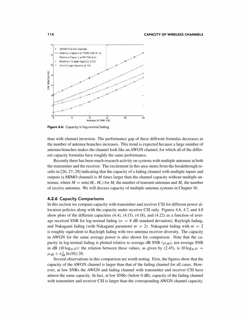
Figure 4.6: Capacity in log-normal fading.

than with channel inversion. The performance gap of these different formulas decreases asthe number of antenna branches increases. This trend is expected because a large number ofantenna branches makes the channel look like an AWGN channel, for which all of the differ-ent capacity formulas have roughly the same performance.

Recently there has been much research activity on systems with multiple antennas at boththe transmitter and the receiver. The excitement in this area stems from the breakthrough re-sults in [26; 27; 28] indicating that the capacity of a fading channel with multiple inputs andoutputs (a MIMO channel) is M times larger than the channel capacity without multiple an-tennas, where M = min(Mt , Mr) for Mt the number of transmit antennas and Mr the numberof receive antennas. We will discuss capacity of multiple antenna systems in Chapter 10.

4.2.6 Capacity ComparisonsIn this section we compare capacity with transmitter and receiver CSI for different power al-location policies along with the capacity under receiver CSI only. Figures 4.6, 4.7, and 4.8show plots of the different capacities (4.4), (4.13), (4.18), and (4.22) as a function of aver-age received SNR for log-normal fading (σ = 8 dB standard deviation), Rayleigh fading,and Nakagami fading (with Nakagami parameter m = 2). Nakagami fading with m = 2is roughly equivalent to Rayleigh fading with two-antenna receiver diversity. The capacityin AWGN for the same average power is also shown for comparison. Note that the ca-pacity in log-normal fading is plotted relative to average dB SNR (μdB), not average SNRin dB (10 log10 μ): the relation between these values, as given by (2.45), is 10 log10 μ =μdB + σ 2

dB ln(10)/20.

Several observations in this comparison are worth noting. First, the figures show that thecapacity of the AWGN channel is larger than that of the fading channel for all cases. How-ever, at low SNRs the AWGN and fading channel with transmitter and receiver CSI havealmost the same capacity. In fact, at low SNRs (below 0 dB), capacity of the fading channelwith transmitter and receiver CSI is larger than the corresponding AWGN channel capacity.


Figure 4.7: Capacity in Rayleigh fading.

Figure 4.8: Capacity in Nakagami fading (m = 2).

That is because the AWGN channel always has the same low SNR, thereby limiting its ca-pacity. A fading channel with this same low average SNR will occasionally have a high SNR,since the distribution has infinite range. Thus, if high power and rate are transmitted over thechannel during these very infrequent large SNR values, the capacity will be greater than onthe AWGN channel with the same low average SNR.

The severity of the fading is indicated by the Nakagami parameter m, where m = 1 forRayleigh fading and m = ∞ for an AWGN channel without fading. Thus, comparing Fig-ures 4.7 and 4.8 we see that, as the severity of the fading decreases (Rayleigh to Nakagamiwith m = 2), the capacity difference between the various adaptive policies also decreases,and their respective capacities approach that of the AWGN channel.


The difference between the capacity curves under transmitter and receiver CSI (4.13) andreceiver CSI only (4.4) are negligible in all cases. Recalling that capacity under receiverCSI only (4.4) and under transmitter and receiver CSI without power adaptation (4.7) arethe same, we conclude that, if the transmission rate is adapted relative to the channel, thenadapting the power as well yields a negligible capacity gain. It also indicates that transmitteradaptation yields a negligible capacity gain relative to using only receiver side information.In severe fading conditions (Rayleigh and log-normal fading), maximum outage capacityexhibits a 1–5-dB rate penalty and zero-outage capacity yields a large capacity loss relativeto Shannon capacity. However, under mild fading conditions (Nakagami with m = 2) theShannon, maximum outage, and zero-outage capacities are within 3 dB of each other andwithin 4 dB of the AWGN channel capacity. These differences will further decrease as thefading diminishes (m → ∞ for Nakagami fading).

We can view these results as a trade-off between capacity and complexity. The adaptivepolicy with transmitter and receiver side information requires more complexity in the trans-mitter (and typically also requires a feedback path between the receiver and transmitter toobtain the side information). However, the decoder in the receiver is relatively simple. Thenonadaptive policy has a relatively simple transmission scheme, but its code design must usethe channel correlation statistics (often unknown) and the decoder complexity is proportionalto the channel decorrelation time. The channel inversion and truncated inversion policies usecodes designed for AWGN channels and thus are the least complex to implement, but in se-vere fading conditions they exhibit large capacity losses relative to the other techniques.

In general, Shannon capacity analysis does not show how to design adaptive or non-adaptive techniques for real systems. Achievable rates for adaptive trellis-coded MQAMhave been investigated in [24], where a simple four-state trellis code combined with adaptivesix-constellation MQAM modulation was shown to achieve rates within 7 dB of the Shan-non capacity (4.9) in Figures 4.6 and 4.7. More complex codes further close the gap to theShannon limit of fading channels with transmitter adaptation.

4.3 Capacity of Frequency-Selective Fading Channels

In this section we examine the Shannon capacity of frequency-selective fading channels. Wefirst consider the capacity of a time-invariant frequency-selective fading channel. This ca-pacity analysis is like that of a flat fading channel but with the time axis replaced by thefrequency axis. Then we discuss the capacity of time-varying frequency-selective fadingchannels.

4.3.1 Time-Invariant ChannelsConsider a time-invariant channel with frequency response H(f ), as shown in Figure 4.9.Assume a total transmit power constraint P. When the channel is time invariant it is typ-ically assumed that H(f ) is known to both the transmitter and receiver. (The capacity oftime-invariant channels under different assumptions about channel knowledge are discussedin [19; 21].)

Let us first assume that H(f ) is block fading, so that frequency is divided into subchannelsof bandwidth B with H(f ) = Hj constant over each subchannel, as shown in Figure 4.10.

4.3 CAPACITY OF FREQUENCY-SELECTIVE FADING CHANNELS 117

Figure 4.9: Time-invariant frequency-selective fading channel.

Figure 4.10: Block frequency-selective fading.

The frequency-selective fading channel thus consists of a set of AWGN channels in paral-lel with SNR |Hj |2Pj/N0B on the j th channel, where Pj is the power allocated to the j thchannel in this parallel set subject to the power constraint

∑j Pj ≤ P.

The capacity of this parallel set of channels is the sum of rates on each channel withpower optimally allocated over all channels [5; 6]:

C =∑

max Pj :∑

j Pj ≤P

B log2

(1 + |Hj |2Pj

N0B

). (4.23)

Note that this is similar to the capacity and optimal power allocation for a flat fading chan-nel, with power and rate changing over frequency in a deterministic way rather than overtime in a probabilistic way. The optimal power allocation is found via the same Lagrangiantechnique used in the flat-fading case, which leads to the water-filling power allocation

Pj

P=

{1/γ0 − 1/γj γj ≥ γ0,

0 γj < γ0,(4.24)

for some cutoff value γ0, where γj = |Hj |2P/N0B is the SNR associated with the j th channelassuming it is allocated the entire power budget. This optimal power allocation is illustratedin Figure 4.11. The cutoff value is obtained by substituting the power adaptation formula intothe power constraint, so γ0 must satisfy

∑

j

(1

γ0− 1

γj

)= 1. (4.25)


Figure 4.11: Water-filling in frequency-selective block fading.

The capacity then becomes

C =∑

j :γj ≥γ0

B log2

(γj

γ0

). (4.26)

This capacity is achieved by transmitting at different rates and powers over each subchannel.Multicarrier modulation uses the same technique in adaptive loading, as discussed in moredetail in Section 12.3.

When H(f ) is continuous, the capacity under power constraint P is similar to the case ofthe block fading channel, with some mathematical intricacies needed to show that the chan-nel capacity is given by

C = maxP(f ):

∫P(f ) df ≤P

∫log2

(1 + |H(f )|2P(f )

N0

)df. (4.27)

The expression inside the integral can be thought of as the incremental capacity associatedwith a given frequency f over the bandwidth df with power allocation P(f ) and channel gain|H(f )|2. This result is formally proven using a Karhunen–Loeve expansion of the channelh(t) to create an equivalent set of parallel independent channels [5, Chap. 8.5]. An alternateproof [29] decomposes the channel into a parallel set using the discrete Fourier transform(DFT); the same premise is used in the discrete implementation of multicarrier modulationdescribed in Section 12.4.

The power allocation over frequency, P(f ), that maximizes (4.27) is found via the La-grangian technique. The resulting optimal power allocation is water-filling over frequency:

P(f )

P=

{1/γ0 − 1/γ (f ) γ (f ) ≥ γ0,

0 γ (f ) < γ0,(4.28)

where γ (f ) = |H(f )|2P/N0. This results in channel capacity

C =∫

f :γ (f )≥γ0

log2

(γ (f )

γ0

)df. (4.29)

4.3 CAPACITY OF FREQUENCY-SELECTIVE FADING CHANNELS 119

Figure 4.12: Channel division in frequency-selective fading.

EXAMPLE 4.7: Consider a time-invariant frequency-selective block fading channelthat has three subchannels of bandwidth B = 1 MHz. The frequency responses as-sociated with each subchannel are H1 = 1, H2 = 2, and H3 = 3, respectively. Thetransmit power constraint is P = 10 mW and the noise PSD N0/2 has N0 = 10−9

W/Hz. Find the Shannon capacity of this channel and the optimal power allocationthat achieves this capacity.

Solution: We first find γj = |Hj |2P/N0B for each subchannel, yielding γ1 = 10, γ2 =40, and γ3 = 90. The cutoff γ0 must satisfy (4.25). Assuming that all subchannelsare allocated power, this yields

3

γ0= 1 +

∑

j

1

γj

= 1.14 �⇒ γ0 = 2.64 < γj ∀j.

Since the cutoff γ0 is less than γj for all j, our assumption that all subchannels areallocated power is consistent, so this is the correct cutoff value. The correspondingcapacity is C = ∑3

j=1 B log2(γj/γ0) = 1000000(log2(10/2.64) + log2(40/2.64) +log2(90/2.64)) = 10.93 Mbps.

4.3.2 Time-Varying ChannelsThe time-varying frequency-selective fading channel is similar to the model shown in Fig-ure 4.9 except that H(f ) = H(f , i); that is, the channel varies over both frequency and time.It is difficult to determine the capacity of time-varying frequency-selective fading channels –even when the instantaneous channel H(f , i) is known perfectly at the transmitter and re-ceiver – because of the effects of self-interference (ISI). In the case of transmitter and receiverside information, the optimal adaptation scheme must consider (a) the effect of the channelon the past sequence of transmitted bits and (b) how the ISI resulting from these bits willaffect future transmissions [30]. The capacity of time-varying frequency-selective fadingchannels is in general unknown, but there do exist upper and lower bounds as well as limitingformulas [30; 31].

We can approximate channel capacity in time-varying frequency-selective fading by tak-ing the channel bandwidth B of interest and then dividing it up into subchannels the size ofthe channel coherence bandwidth Bc, as shown in Figure 4.12. We then assume that each of


the resulting subchannels is independent, time varying, and flat fading with H(f , i) = Hj [i]on the j th subchannel.

Under this assumption, we obtain the capacity for each of these flat fading subchannelsbased on the average power Pj that we allocate to each subchannel, subject to a total powerconstraint P. Since the channels are independent, the total channel capacity is just equal tothe sum of capacities on the individual narrowband flat fading channels – subject to the totalaverage power constraint and averaged over both time and frequency:

C = max{Pj}:

∑j Pj ≤P

∑

j

Cj(Pj ), (4.30)

where Cj(Pj ) is the capacity of the flat fading subchannel with average power Pj and band-width Bc given by (4.13), (4.4), (4.18), or (4.22) for Shannon capacity under different sideinformation and power allocation policies. We can also define Cj(Pj ) as a capacity versusoutage if only the receiver has side information.

We will focus on Shannon capacity assuming perfect transmitter and receiver channel CSI,since this upperbounds capacity under any other side information assumptions or suboptimalpower allocation strategies. We know that if we fix the average power per subchannel thenthe optimal power adaptation follows a water-filling formula. We expect that the optimalaverage power to be allocated to each subchannel will also follow a water-filling formula,where more average power is allocated to better subchannels. Thus we expect that the opti-mal power allocation is a two-dimensional water-filling in both time and frequency. We nowobtain this optimal two-dimensional water-filling and the corresponding Shannon capacity.

Define γj [i] = |Hj [i]|2P/N0B to be the instantaneous SNR on the j th subchannel at timei assuming the total power P is allocated to that time and frequency. We allow the powerPj(γj ) to vary with γj [i]. The Shannon capacity with perfect transmitter and receiver CSI isgiven by optimizing power adaptation relative to both time (represented by γj [i] = γj ) andfrequency (represented by the subchannel index j):

C = maxPj(γj ):

∑j

∫ ∞0

Pj(γj )p(γj ) dγj ≤P

∑

j

∫ ∞

0Bc log2

(1 + Pj(γj )γj

P

)p(γj ) dγj . (4.31)

To find the optimal power allocation Pj(γj ), we form the Lagrangian

J(Pj(γj ))

=∑

j

∫ ∞

0Bc log2

(1 + Pj(γj )γj

P

)p(γj ) dγj − λ

∑

j

∫ ∞

0Pj(γj )p(γj ) dγj . (4.32)

Note that (4.32) is similar to the Lagrangian (4.10) for the flat fading channel except that thedimension of frequency has been added by summing over the subchannels. Differentiatingthe Lagrangian and setting this derivative equal to zero eliminates all terms except the givensubchannel and associated SNR:

∂J(Pj(γj ))

∂Pj(γj )=

[(Bc/ln(2)

1 + γjPj(γj )/P

)γj

P− λ

]p(γj ) = 0. (4.33)

PROBLEMS 121

Solving for Pj(γj ) yields the same water-filling as the flat-fading case:

Pj(γj )

P=

{1/γ0 − 1/γj γj ≥ γ0,

0 γj < γ0,(4.34)

where the cutoff value γ0 is obtained from the total power constraint over both time andfrequency:

∑

j

∫ ∞

0Pj(γj )p(γj ) dγj = P. (4.35)

Thus, the optimal power allocation (4.34) is a two-dimensional water-filling with a commoncutoff value γ0. Dividing the constraint (4.35) by P and substituting into the optimal powerallocation (4.34), we get that γ0 must satisfy

∑

j

∫ ∞

γ0

(1

γ0− 1

γj

)p(γj ) dγj = 1. (4.36)

It is interesting to note that, in the two-dimensional water-filling, the cutoff value for allsubchannels is the same. This implies that even if the fading distribution or average fadepower on the subchannels is different, all subchannels suspend transmission when the in-stantaneous SNR falls below the common cutoff value γ0. Substituting the optimal powerallocation (4.35) into the capacity expression (4.31) yields

C =∑

j

∫ ∞

γ0

Bc log2

(γj

γ0

)p(γj ) dγj . (4.37)

PROBLEMS

4-1. Capacity in AWGN is given by C = B log2(1 + P/N0B), where P is the received sig-nal power, B is the signal bandwidth, and N0/2 is the noise PSD. Find capacity in the limitof infinite bandwidth B → ∞ as a function of P.

4-2. Consider an AWGN channel with bandwidth 50 MHz, received signal power 10 mW,and noise PSD N0/2 where N0 = 2 · 10−9 W/Hz. How much does capacity increase bydoubling the received power? How much does capacity increase by doubling the channelbandwidth?

4-3. Consider two users simultaneously transmitting to a single receiver in an AWGN chan-nel. This is a typical scenario in a cellular system with multiple users sending signals toa base station. Assume the users have equal received power of 10 mW and total noise atthe receiver in the bandwidth of interest of 0.1 mW. The channel bandwidth for each user is20 MHz.

(a) Suppose that the receiver decodes user 1’s signal first. In this decoding, user 2’s sig-nal acts as noise (assume it has the same statistics as AWGN). What is the capacityof user 1’s channel with this additional interference noise?


(b) Suppose that, after decoding user 1’s signal, the decoder re-encodes it and subtractsit out of the received signal. Now, in the decoding of user 2’s signal, there is no inter-ference from user 1’s signal. What then is the Shannon capacity of user 2’s channel?

Note: We will see in Chapter 14 that the decoding strategy of successively subtracting outdecoded signals is optimal for achieving Shannon capacity of a multiuser channel with inde-pendent transmitters sending to one receiver.

4-4. Consider a flat fading channel of bandwidth 20 MHz and where, for a fixed transmitpower P, the received SNR is one of six values: γ1 = 20 dB, γ2 = 15 dB, γ3 = 10 dB, γ4 =5 dB, γ5 = 0 dB, and γ6 = −5 dB. The probabilities associated with each state are p1 =p6 = .1, p2 = p4 = .15, and p3 = p5 = .25. Assume that only the receiver has CSI.

(a) Find the Shannon capacity of this channel.(b) Plot the capacity versus outage for 0 ≤ Pout < 1 and find the maximum average rate

that can be correctly received (maximum Cout).

4-5. Consider a flat fading channel in which, for a fixed transmit power P, the received SNRis one of four values: γ1 = 30 dB, γ2 = 20 dB, γ3 = 10 dB, and γ4 = 0 dB. The probabili-ties associated with each state are p1 = .2, p2 = .3, p3 = .3, and p4 = .2. Assume that bothtransmitter and receiver have CSI.

(a) Find the optimal power adaptation policy P [i]/P for this channel and its correspond-ing Shannon capacity per unit hertz (C/B).

(b) Find the channel inversion power adaptation policy for this channel and associatedzero-outage capacity per unit bandwidth.

(c) Find the truncated channel inversion power adaptation policy for this channel and as-sociated outage capacity per unit bandwidth for three different outage probabilities:Pout = .1, Pout = .25, and Pout (and the associated cutoff γ0) equal to the value thatachieves maximum outage capacity.

4-6. Consider a cellular system where the power falloff with distance follows the formulaPr(d ) = Pt(d0/d )α, where d0 = 100 m and α is a random variable. The distribution for α isp(α = 2) = .4, p(α = 2.5) = .3, p(α = 3) = .2, and p(α = 4) = .1. Assume a receiverat a distance d = 1000 m from the transmitter, with an average transmit power constraint ofPt = 100 mW and a receiver noise power of .1 mW. Assume that both transmitter and receiverhave CSI.

(a) Compute the distribution of the received SNR.(b) Derive the optimal power adaptation policy for this channel and its corresponding

Shannon capacity per unit hertz (C/B).

(c) Determine the zero-outage capacity per unit bandwidth of this channel.(d) Determine the maximum outage capacity per unit bandwidth of this channel.

4-7. Assume a Rayleigh fading channel, where the transmitter and receiver have CSI and thedistribution of the fading SNR p(γ ) is exponential with mean γ = 10 dB. Assume a channelbandwidth of 10 MHz.

(a) Find the cutoff value γ0 and the corresponding power adaptation that achieves Shan-non capacity on this channel.

PROBLEMS 123

Figure 4.13: Interference channel for Problem 4-8.

(b) Compute the Shannon capacity of this channel.(c) Compare your answer in part (b) with the channel capacity in AWGN with the same

average SNR.(d) Compare your answer in part (b) with the Shannon capacity when only the receiver

knows γ [i].(e) Compare your answer in part (b) with the zero-outage capacity and outage capacity

when the outage probability is .05.(f ) Repeat parts (b), (c), and (d) – that is, obtain the Shannon capacity with perfect trans-

mitter and receiver side information, in AWGN for the same average power, and withjust receiver side information – for the same fading distribution but with mean γ =−5 dB. Describe the circumstances under which a fading channel has higher capac-ity than an AWGN channel with the same average SNR and explain why this behavioroccurs.

4-8. This problem illustrates the capacity gains that can be obtained from interference esti-mation and also how a malicious jammer can wreak havoc on link performance. Considerthe interference channel depicted in Figure 4.13. The channel has a combination of AWGNn[k] and interference I [k]. We model I [k] as AWGN. The interferer is on (i.e., the switch isdown) with probability .25 and off (i.e., switch up) with probability .75. The average trans-mit power is 10 mW, the noise PSD has N0 = 10−8 W/Hz, the channel bandwidth B is 10 kHz(receiver noise power is N0B), and the interference power (when on) is 9 mW.

(a) What is the Shannon capacity of the channel if neither transmitter nor receiver knowwhen the interferer is on?

(b) What is the capacity of the channel if both transmitter and receiver know when theinterferer is on?

(c) Suppose now that the interferer is a malicious jammer with perfect knowledge of x[k](so the interferer is no longer modeled as AWGN). Assume that neither transmitternor receiver has knowledge of the jammer behavior. Assume also that the jammeris always on and has an average transmit power of 10 mW. What strategy should thejammer use to minimize the SNR of the received signal?

4-9. Consider the malicious interferer of Problem 4-8. Suppose that the transmitter knowsthe interference signal perfectly. Consider two possible transmit strategies under this sce-nario: the transmitter can ignore the interference and use all its power for sending its signal,or it can use some of its power to cancel out the interferer (i.e., transmit the negative of the


interference signal). In the first approach the interferer will degrade capacity by increasing thenoise, and in the second strategy the interferer also degrades capacity because the transmittersacrifices some power to cancel out the interference. Which strategy results in higher capac-ity? Note: There is a third strategy, in which the encoder actually exploits the structure of theinterference in its encoding. This strategy is called dirty paper coding and is used to achieveShannon capacity on broadcast channels with multiple antennas, as described in Chapter 14.

4-10. Show using Lagrangian techniques that the optimal power allocation to maximize thecapacity of a time-invariant block fading channel is given by the water-filling formula in(4.24).

4-11. Consider a time-invariant block fading channel with frequency response

H(f ) =

⎧⎪⎪⎪⎪⎨

⎪⎪⎪⎪⎩

1 fc − 20 MHz ≤ f < fc − 10 MHz,.5 fc − 10 MHz ≤ f < fc,2 fc ≤ f < fc + 10 MHz,.25 fc + 10 MHz ≤ f < fc + 20 MHz,0 else,

for f > 0 and H(−f ) = H(f ). For a transmit power of 10 mW and a noise PSD of .001μWper Hertz, find the optimal power allocation and corresponding Shannon capacity of thischannel.

4-12. Show that the optimal power allocation to maximize the capacity of a time-invariantfrequency-selective fading channel is given by the water-filling formula in (4.28).

4-13. Consider a frequency-selective fading channel with total bandwidth 12 MHz and co-herence bandwidth Bc = 4 MHz. Divide the total bandwidth into three subchannels of band-width Bc, and assume that each subchannel is a Rayleigh flat fading channel with independentfading on each subchannel. Assume the subchannels have average gains E[|H1[i]|2] = 1,E[|H2[i]|2] = .5, and E[|H3[i]|2] = .125. Assume a total transmit power of 30 mW and areceiver noise PSD with N0 = .001μW/Hz.

(a) Find the optimal two-dimensional water-filling power adaptation for this channel andthe corresponding Shannon capacity, assuming both transmitter and receiver knowthe instantaneous value of Hj[i], j = 1, 2, 3.

(b) Compare the capacity derived in part (a) with that obtained by allocating an equal av-erage power of 10 mW to each subchannel and then water-filling on each subchannelrelative to this power allocation.

REFERENCES

[1] C. E. Shannon, “A mathematical theory of communication,” Bell System Tech. J., pp. 379–423,623–56, 1948.

[2] C. E. Shannon, “Communications in the presence of noise.” Proc. IRE, pp. 10–21, 1949.[3] C. E. Shannon and W. Weaver, The Mathematical Theory of Communication, University of Illi-

nois Press, Urbana, 1949.[4] M. Medard, “The effect upon channel capacity in wireless communications of perfect and im-

perfect knowledge of the channel,” IEEE Trans. Inform. Theory, pp. 933–46, May 2000.[5] R. G. Gallager, Information Theory and Reliable Communication, Wiley, New York, 1968.[6] T. Cover and J. Thomas, Elements of Information Theory, Wiley, New York, 1991.

REFERENCES 125

[7] C. Heegard and S. B. Wicker, Turbo Coding, Kluwer, Boston, 1999.[8] I. Csiszár and J. Kórner, Information Theory: Coding Theorems for Discrete Memoryless Chan-

nels, Academic Press, New York, 1981.[9] I. Csiszár and P. Narayan, “The capacity of the arbitrarily varying channel,” IEEE Trans. Inform.

Theory, pp. 18–26, January 1991.[10] I. C. Abou-Faycal, M. D. Trott, and S. Shamai, “The capacity of discrete-time memoryless

Rayleigh fading channels,” IEEE Trans. Inform. Theory, pp. 1290–1301, May 2001.[11] A. Lapidoth and S. M. Moser, “Capacity bounds via duality with applications to multiple-antenna

systems on flat-fading channels,” IEEE Trans. Inform. Theory, pp. 2426–67, October 2003.[12] A. J. Goldsmith and P. P. Varaiya, “Capacity, mutual information, and coding for finite-state

Markov channels,” IEEE Trans. Inform. Theory, pp. 868–86, May 1996.[13] M. Mushkin and I. Bar-David, “Capacity and coding for the Gilbert–Elliot channel,” IEEE Trans.

Inform. Theory, pp. 1277–90, November 1989.[14] T. Holliday, A. Goldsmith, and P. Glynn, “Capacity of finite state Markov channels with general

inputs,” Proc. IEEE Internat. Sympos. Inform. Theory, p. 289, July 2003.[15] R. J. McEliece and W. E. Stark, “Channels with block interference,” IEEE Trans. Inform. The-

ory, pp. 44–53, January 1984.[16] A. Lapidoth and S. Shamai, “Fading channels: How perfect need ‘perfect side information’ be?”

IEEE Trans. Inform. Theory, pp. 1118–34, November 1997.[17] G. J. Foschini, D. Chizhik, M. Gans, C. Papadias, and R. A. Valenzuela, “Analysis and perfor-

mance of some basic space-time architectures,” IEEE J. Sel. Areas Commun., pp. 303–20, April2003.

[18] W. L. Root and P. P. Varaiya, “Capacity of classes of Gaussian channels,” SIAM J. Appl. Math.,pp. 1350–93, November 1968.

[19] J. Wolfowitz, Coding Theorems of Information Theory, 2nd ed., Springer-Verlag, New York,1964.

[20] A. J. Goldsmith and P. P. Varaiya, “Capacity of fading channels with channel side information,”IEEE Trans. Inform. Theory, pp. 1986–92, November 1997.

[21] G. Caire and S. Shamai, “On the capacity of some channels with channel state information,”IEEE Trans. Inform. Theory, pp. 2007–19, September 1999.

[22] M.-S. Alouini and A. J. Goldsmith, “Capacity of Rayleigh fading channels under different adap-tive transmission and diversity combining techniques,” IEEE Trans. Veh. Tech., pp. 1165–81, July1999.

[23] S.-G. Chua and A. J. Goldsmith, “Variable-rate variable-power MQAM for fading channels,”IEEE Trans. Commun., pp. 1218–30, October 1997.

[24] S.-G. Chua and A. J. Goldsmith, “Adaptive coded modulation for fading channels,” IEEE Trans.Commun., pp. 595–602, May 1998.

[25] K. S. Gilhousen, I. M. Jacobs, R. Padovani, A. J. Viterbi, L. A. Weaver, Jr., and C. E. WheatleyIII, “On the capacity of a cellular CDMA system,” IEEE Trans.Veh.Tech., pp. 303–12, May 1991.

[26] G. J. Foschini, “Layered space-time architecture for wireless communication in fading environ-ments when using multi-element antennas,” Bell System Tech. J., pp. 41–59, Autumn 1996.

[27] E.Teletar, “Capacity of multi-antenna Gaussian channels,”AT&T Bell Labs Internal Tech. Memo,June 1995.

[28] G. J. Foschini and M. Gans, “On limits of wireless communications in a fading environmentwhen using multiple antennas,” Wireless Pers. Commun., pp. 311–35, March 1998.

[29] W. Hirt and J. L. Massey, “Capacity of the discrete-time Gaussian channel with intersymbol in-terference,” IEEE Trans. Inform. Theory, pp. 380–8, May 1988.

[30] A. Goldsmith and M. Medard, “Capacity of time-varying channels with channel side informa-tion,” IEEE Trans. Inform. Theory (to appear).

[31] S. Diggavi, “Analysis of multicarrier transmission in time-varying channels,” Proc. IEEE Inter-nat. Conf. Commun., pp. 1191–5, June 1997.

Capacity of Wireless Channels -...

Documents

Transcript of Capacity of Wireless Channels -...