Technical Report Documentation Page 1. Report No. FHWA/TX-09/0-5619-1

2. Government Accession No.

3. Recipient's Catalog No.

4. Title and Subtitle CAPACITY AND ROAD USER COST ANALYSIS OF SELECTED

REEWAY WORK ZONES IN TEXAS F

5. Report Date September 2009 Published: September 2009 6. Performing Organization Code

7. Author(s) Darrell W. Borchardt, Geza Pesti, Dazhi Sun, and Liang Ding

8. Performing Organization Report No. Report 0-5619-1

9. Performing Organization Name and Address Texas Transportation Institute The Texas A&M University System College Station, Texas 77843-3135

10. Work Unit No. (TRAIS) 11. Contract or Grant No. Project 0-5619

12. Sponsoring Agency Name and Address Texas Department of Transportation Research and Technology Implementation Office P.O. Box 5080 A ustin, Texas 78763-5080

13. Type of Report and Period Covered Technical Report: September 2006-August 2008 14. Sponsoring Agency Code

15. Supplementary Notes Project performed in cooperation with the Texas Department of Transportation and the Federal Highway Administration. Project Title: Updated Work Zone Capacities URL: http://tti.tamu.edu/documents/0-5619-1.pdf 16. Abstract This research was developed to produce usable and meaningful estimates for work zone capacities under a variety of roadway and traffic conditions, work zone configurations, and lane closure scenarios within Texas. Using data collected at eighteen work zone sites, the research presents updated guidance for expected capacities of various freeway work zone lane closure configurations. In addition, models used to evaluate traffic conditions in work zones were evaluated and recommendations for their use were made. Finally, recommendations concerning road user cost analysis for freeway construction projects are included. 17. Key Words Work Zone, Capacity, Road User Cost, Freeway

18. Distribution Statement No restrictions. This document is available to the public through NTIS: National Technical Information Service Springfield, Virginia 22161 http://www.ntis.gov

19. Security Classif.(of this report) Unclassified

20. Security Classif.(of this page) Unclassified

21. No. of Pages 78

22. Price

Form DOT F 1700.7 (8-72) Reproduction of completed page authorized

CAPACITY AND ROAD USER COST ANALYSIS OF SELECTED FREEWAY WORK ZONES IN TEXAS

by

Darrell W. Borchardt, P.E. Senior Research Engineer

Texas Transportation Institute

Geza Pesti, Ph.D., P.E. Associate Research Engineer Texas Transportation Institute

Dazhi Sun, Ph.D.

Assistant Professor Texas A&M University-Kingsville

and

Liang Ding

Assistant Transportation Researcher Texas Transportation Institute

Report 0-5619-1 Project 0-5619

Project Title: Updated Work Zone Capacities

Performed in cooperation with the Texas Department of Transportation

and the Federal Highway Administration

September 2009 Published: September 2009

TEXAS TRANSPORTATION INSTITUTE The Texas A&M University System College Station, Texas 77843-3135

DISCLAIMER

This research was performed in cooperation with the Texas Department of Transportation

(TxDOT) and the Federal Highway Administration (FHWA). The contents of this report reflect

the views of the authors, who are responsible for the facts and the accuracy of the data presented

herein. The contents do not necessarily reflect the official view or policies of the FHWA or

TxDOT. This report does not constitute a standard, specification, or regulation.

This report is not intended for construction, bidding, or permit purposes. The engineer in

charge of the project was Darrell W. Borchardt, P.E. #62074.

The United States Government and the State of Texas do not endorse products or

manufacturers. Trade or manufacturers’ names appear herein solely because they are considered

essential to the object of this report.

v

ACKNOWLEDGMENTS

This project was conducted in cooperation with TxDOT and FHWA. The authors wish

to acknowledge the members of the Project Monitoring Committee without whose insights and

assistance the successful completion of this research project would not have been possible:

• Mr. Craig E. Clark, P.E., TxDOT Corpus Christi District, Program Coordinator;

• Mr. Ismael C. Soto, P.E., TxDOT Corpus Christi District, Project Director;

• Ms. Marla M. Jasek, P.E., TxDOT Yoakum District, Project Advisor;

• Mr. Andrew R. Oberlander, P.E., TxDOT Dallas District, Project Advisor;

• Mr. Ray Z. Thomasian, P.E., TxDOT Design Division, Project Advisor;

• Mr. David Valdez, P.E., TxDOT Traffic Operations Division, Project Advisor; and

• Mr. Wade Odell, P.E., TxDOT Research and Technology Implementation Office,

Research Engineer.

The authors also wish to acknowledge the assistance of Jinpeng Lv and Anxi Jia, both

Graduate Assistants at Texas A&M University-Kingsville. Their assistance in data reduction

and analysis throughout the project was an important factor in the completion of this research.

vi

TABLE OF CONTENTS

Page List of Figures ............................................................................................................................. viii List of Tables ................................................................................................................................ ix Chapter 1. Introduction............................................................................................................... 1 

Definition of Work Zone Capacity ............................................................................................. 1 Literature Review of Work Zone Capacity Estimation .............................................................. 2 Estimation of Work Zone Capacities .......................................................................................... 2 Factors Impacting Work Zone Capacity ..................................................................................... 8 Road User Cost Estimation in Work Zones ................................................................................ 9 

Chapter 2. Survey of Current Practices in Texas ................................................................... 13 Chapter 3. Field Measurement of Work Zone Capacity ........................................................ 19 

Strategy for Site Selection ........................................................................................................ 19 Results of Field Studies ............................................................................................................ 21 

Chapter 4. Validation of Simulation Models ........................................................................... 25 “Linear” Models ........................................................................................................................ 25 

QUEWZ-92 ........................................................................................................................... 25 Highway Capacity Software (HCS+).................................................................................... 27 Kim’s Multiple Regression Model ........................................................................................ 28 MicroBENCOST................................................................................................................... 29 

“Network” Models .................................................................................................................... 30 QuickZone............................................................................................................................. 30 VISSIM ................................................................................................................................. 31 CA4PRS ................................................................................................................................ 32 

Comparison of Model Outputs.................................................................................................. 32 Chapter 5. Road User Cost Analsyis ........................................................................................ 35 Chapter 6. Emissions in Work Zones ....................................................................................... 39 Chapter 7. Findings and Recommendations ........................................................................... 41 References .................................................................................................................................... 43 Appendix A. Description of Field Study Sites ......................................................................... 47 Appendix B. Summary of Data Input for Model Validation ................................................. 65 Appendix C. Summary of Road User Cost Model Comparison ............................................ 67 

vii

LIST OF FIGURES

Page Figure 1. Survey Structure. .......................................................................................................... 13 Figure 2. Email Survey. ............................................................................................................... 14 Figure 3. Survey Results: Guidelines to Estimate Work Zone Capacity. ................................... 15 Figure 4. Surveys Results: Software to Estimate Work Zone Capacity. .................................... 16 Figure 5. Survey Results: Factors Affecting Work Zone Capacity. ........................................... 17 Figure 6. Initial Matrix of Study Site Design. ............................................................................. 19 Figure 7. Total Emission for Both Normal and Work Zone Condition. ...................................... 39 

viii

ix

LIST OF TABLES

Page Table 1. Major Freeway Constructions Listed by Districts. ........................................................ 18 Table 2. Summary of Maximum Work Zone Volumes. .............................................................. 22 Table 3. Capacity Comparison. .................................................................................................... 33 Table 4. Comparison of Road User Costs for San Antonio Work Zones. ................................... 38 

CHAPTER 1. INTRODUCTION

As traffic demand on Texas roadways continues to increase, the state must allocate

substantial resources to constructing new roadways as well as maintaining the existing

infrastructure. Roadway construction projects are among the most visible activities that the

Texas Department of Transportation (TxDOT) completes for the traveling public. Freeway work

zones, which typically include closed or narrowed lanes, may cause disruptions to normal traffic

flow. These roadway sections with reduced capacities may cause traffic delays resulting in

increased road user costs, traffic incidents, and vehicle emissions. The public desires the

projects to be completed as quickly as possible with minimal impact on daily travels. In order to

assure the quickest project completion minimizes the impacts of freeway work zones, TxDOT

constructs most major projects using incentives for early completion and/or liquidated damages

for failure to meet the contractual deadlines. Lane assessments or lane rental fees on routine

maintenance contracts as well as for standard roadway construction projects are also being used.

A critical input into the analysis process for determining the dollar amount of incentive, penalty,

or lane rental assessment is the use of accurate roadway capacity for roadway segments impacted

by the construction project. In addition to the updated capacity values being used in road user

cost studies, TxDOT staff uses these capacity values to quantify the traffic carrying capacity of

various work zone configurations using traffic control plan development such that delay to the

public will be minimized.

Although there have been previous research studies examining work zone capacity

estimation, many of these studies are outdated and may not accurately represent current travel

conditions on Texas roadways. This project, which was a joint venture between the Texas

Transportation Institute (TTI) and Texas A&M University-Kingsville, was developed to update

capacity values in Texas work zones and to evaluate traffic models for estimating road user

costs.

DEFINITION OF WORK ZONE CAPACITY

The Highway Capacity Manual 2000 (HCM 2000) defines capacity as: “The maximum

sustainable flow rate at which vehicles or persons reasonably can be expected to traverse a point

or uniform segment of a lane or roadway during a specified time period under given roadway,

1

geometric, traffic, environmental, and control conditions; usually expressed as vehicles per hour,

passenger cars per hour, or persons per hour (1).”

There are two different approaches to measuring the capacities of freeway work zones.

The first considers the work zone capacity as the largest traffic volume as measured through the

construction area. In practice, this value is generally accepted as the peak 15-minute traffic flow

rate. However, some studies consider this volume as unsustainable for a significant time period.

Traffic volume measured in a work zone during congestion is usually the flow rate of the queued

vehicles being discharged from the work zone. Thus, the second approach considers the queue-

discharge rate of the work zone as the basis for capacity estimation. Some criteria to identify the

work zone capacity in previous studies are as follows:

• the flow rate derived from three-minute time intervals during congested conditions

(California) (2);

• the hourly traffic volume under congested traffic conditions (Texas) (3);

• the flow rate at which traffic conditions quickly changed from uncongested to queue

conditions (North Carolina) (4);

• the maximum recorded five-minute flow rate (Pennsylvania) (5);

• the flow rate just before a sharp speed drop (Indiana) (5); and

• the highest flow sustained during a 15-minute time period that is either before a rapid

speed drop or after a rapid speed increase (Illinois) (6).

LITERATURE REVIEW OF WORK ZONE CAPACITY ESTIMATION

The objective of this literature review is to provide a comprehensive examination of work

zone capacity estimation methods that may be used to configure lane closures, minimize traffic

delay, and manage road user costs. The literature review had three major focus areas:

• estimation of work zone capacities,

• factors impacting work zone capacity,

• delay and road user cost estimation.

ESTIMATION OF WORK ZONE CAPACITIES

Widespread traffic growth has prompted the need for roadway improvements in most

sectors of urban roadway systems. This growth combined with the accompanying construction

2

to accommodate the need for expanded roadway capabilities has necessitated the need for an

accurate methodology to predict work-zone capacity in areas of construction and maintenance.

The impact of work-zones depends not only on the traffic itself, but also the effect of lane

closures, construction intensity, and multiple other factors. In order to reduce the negative

effects of work-zone activities, careful management, accurate planning and the ability to reliably

estimate work-zone capacities are required.

The ability to accurately estimate work-zone capacity is imperative, as it is a key input to

queue length, delay, and delay costs estimations. Several factors, such as driver population,

vehicle composition (truck percentage), light conditions (day or night), weather conditions,

intensity of work activity, lane closure configuration, lane width, roadway terrain, and gradient,

must be considered in estimating work zone capacity. Some of these factors are easily measured,

whereas others have to be estimated.

Based on research by the Texas Transportation Institute leading to the release of the

Highway Capacity Manual of 1985 (7), researchers developed an empirical method of estimating

freeway work-zone capacity. This methodology was improved upon so that by the release of the

Highway Capacity Manual 2000 (1), this technique had become a standard method used by

transportation departments and agencies in estimating the capacity of work zones with lane

closures. The Highway Capacity Manual 2000 (1) takes the unrestricted base capacity of 1,600

vehicles per hour per lane (vphpl) used for work zone areas without flow restrictions and

modifies it by using multiple reduction factors. This modified value takes into account

parameters such as lane width, percentage of heavy vehicles, work intensity and proximity of

ramps.

A number of studies have focused on the improvement of work-zone capacity estimation

methods. In a recent paper (8), research efforts to improve the estimation of the effects of lane

closures at freeway maintenance and construction zones were reviewed. In the early 1990s,

Krammes and Lopez (9) developed new guidelines for estimating capacity for various types of

lane closure configurations and introduced updated higher capacity values for short-term work

zone lane closures.

Based on field data, Abrams and Wang (10) developed a model that combines the HCM

2000 adjustment factors with a new factor that considers work duration. Dudek et al. (11, 12)

developed the computer model QUEWZ to estimate capacity by classifying various lane closure

3

configurations and applying a regression analysis. QUEWZ was then improved by integrating

additional factors considering work zone intensity, percentage of heavy vehicle presence, and the

location of entrance ramps.

Kim, Lovell, and Paracha (8) developed a new capacity estimation methodology based on

an expanded assessment of a number of factors. These factors included the number of open and

closed lanes, location of the closed lanes, heavy vehicle percentage, driver population, entrance

ramp volume, width of open lanes, and the length and grade of the work zone. Additional factors

included the intensity of the work activity, project duration, weather conditions, and the time of

day when work is performed. This new methodology with the newly determined key factors

proved more accurate at predicting capacity than the models they reviewed in their study.

In another study by Al-Kaisy and Hall (13), two-step guidelines for estimating capacity at

freeway reconstruction zones were introduced. In the first step, the effect of heavy vehicles,

driver population, weather, site configuration, work activity, and light conditions on capacity was

examined. This study suggested that heavy vehicles and driver population were the most

significant factors affecting work zone capacity. In the second step, two separate capacity

models are offered, one being a generic model and the other a site-specific model.

One of the capacity estimation methods is the multiplicative capacity model. It accounts

for several independent factors that may affect work zone capacity and uses appropriate

adjustments to reduce an ideal base work zone capacity (13). The multiplicative model also used

by the HCM 2000 (1) uses the following formula and adjustment factors:

rswddHVb ffffffCC ××××××= 21

where,

C = the work zone capacity (vphpl);

Cb = ideal base work zone capacity (passenger cars per hour per lane) (pcphpl);

fd1 = off-peak weekday driver population (off-peak=fd1, else=1);

fd2 = weekend driver population (weekend=fd2, else=1);

fw = work activity (no work activity=1);

fs = side of lane closure (left lane closed=fs, right lane closed=1);

fr = rain (rain = fr, no rain=1); and

fHV = heavy vehicle (see formula below).

4

[ ])1(11

−+=

HVHVHV EP

f

PHV = proportion of heavy vehicles in traffic;

EHV = passenger car equivalency for heavy vehicles.

Al-Kaisy and Hall (13) collected field data at several work zones to update the

adjustment factors. A comparison of the base capacity and capacity reduction factors used by the

multiplicative model and those observed in the field are listed below:

Factor Multiplicative Capacity Model Site Findings Base Capacity

Driver Population Weekend Drivers

Work Activity Lane Closure

Rain

2,050 pcphpl 4% reduction

17.5% reduction 3.5% reduction 5.7% reduction 2.5% reduction

2,000 pcphpl 7% reduction 16% reduction

1.85-12.5% reduction 6% reduction

4.4-7.8% reduction

A majority of the values used by the multiplicative capacity model are close to those

observed at the field sites.

Another class of capacity estimation methods, the additive capacity models are based on

multivariate linear regression and incorporate variables similar to those used in the multiplicative

model. In addition to looking at the variables as independent factors, the additive capacity model

examines the interaction between variables. Only the factors showing a significant interaction

effect are included in the additive capacity model. Many widely utilized models belong to this

category, which include the following:

• From Memmott and Dudek (12)

)(CERFbaC −=

where,

C = estimated work zone capacity;

CERF = capacity estimate risk factor suggested in the research; and

a, b = coefficients given in the research.

• From Al-Kaisy and Hall (13)

C = 1964-20.9PHV -82D1–352D2–172W–121S–71R+55SD1+185WD2+58SD2+107RD2

where,

5

C = capacity in vphpl;

PHV = percentage of heavy vehicles in the traffic stream;

D1 = off-peak weekday driver population;

D2 = weekend driver population;

W = work activity at site;

S = side of lane closure;

R = rain (rain=1, else=0);

SD1 = side of lane closure and off-peak weekday driver population;

WD2 = work activity and weekend driver population;

SD2 = side of lane closure and weekend driver population; and

RD2 = rain and weekend driver population.

Researchers concluded that pure multiplicative models or pure additive models could not

predict the capacity accurately, and efforts were made to combine the two kinds of models. The

proposed, so-called “generic” capacity model is a combination of multiplicative and additive

models. The multiplicative model was improved by including the following two factors:

• fl=light condition; and

• fi = nonadditive interactive effects.

Al-Kaisy and Hall first proposed this concept in 2003 (13). Their model had a multiplicative

format, but it also accounted for the interaction between variables just as the additive models.

Other generic capacity models include the following:

• From Krammes and Lopez (9)

N * H * R) - I (1600 C +=

where,

C = estimated work zone capacity;

I = adjustment for type and intensity of work activity suggested in the research;

R = adjustment for presence of ramps suggested in the research;

H = heavy vehicle adjustment factor given in the HCM; and

N= number of lanes open through the work zone.

• From Abrams and Wang (10)

WZF WCF* TF * 2000 C +=

where,

6

C= estimated work zone capacity;

TF = truck adjustment factor given in the HCM;

WCF = lane width and lateral clearance adjustment factor given in the HCM; and

WZF = work zone capacity adjustment factor determined in the research.

• From Kim et al. (8)

C = 1857–168.1NUMCL–37.0LOCCL–9.0HV+92.7LD–34.3WL–106.1WIH–2.3WG*HV

where,

C = estimated work zone capacity;

NUMCL = number of closed lanes;

LOCCL = location of closed lanes;

HV = proportion of heavy vehicles;

LD = lateral distance to the open travel lanes;

WL = work zone length;

WIH = intensity of work zone activity;

WG = work zone grade; and

HV = proportion of heavy vehicles.

• From W. Virgil Ping and Kangyuan Zhu (with interaction effects of two factors) (14)

C = 1619+lane+value(ffs)*wffs+10.2*grade–12.0*truck+truck*lane+grade*lane–

1.97*truck*grade

where,

ffs: free flow speed;

truck: percentage of heavy vehicles;

Lane configuration [number of all lanes, closed lanes] [2,1] [3,2] [3,1] Lane -3.6 177.0 0.0 truck*lane -0.17 -3.95 0.0 grade*lane -0.93 -19.7 0.0

value (ffs) = 0.48 when ffs = 55 mph;

value (ffs) = 0.50 when ffs = 60 mph; and

value (ffs) = 0.55 when ffs = 70 mph.

7

Because of the many interacting variables affecting work zone capacity, it is difficult to

estimate capacity by a simple mathematical formula. Recently, more and more computational

intelligence methods and commercial software have been introduced to help solve this capacity

problem. Jiang and Adeli (15) used a neuro-fuzzy method to quantify factors and develop new

software to estimate the capacity (16). The Neuro-Fuzzy Logic Model introduces a neural

network of interacting variables that are quantified using a fuzzy inference method. This method

accounts for seventeen different variables affecting work zone capacity. A comparison of the

Neuro-Fuzzy Logic Model against two other well known work zone capacity equations, the

Krammes and Lopez’s (1994) empirical method (9) and the multiple-variable regression

equation by Kim et al. (8), the Neuro-Fuzzy Logic Method was found to be more accurate in

most cases than the other two. Also, the Neuro-Fuzzy Logic Model incorporates more factors

than the other models.

The work zone capacity estimator software system called IntelliZone® developed by

Jiang and Adeli (16) is based on pattern recognition and neural network models. IntelliZone uses

seventeen interacting factors in estimating work zone capacity, delay, and queue length. The

main benefit of this model compared to previous models is its ability to examine a variety of

work zone scenarios, multiple roadway segments and various traffic flow strategies. Also

beneficial are its interactive user interface and effective, user-friendly help features.

FACTORS IMPACTING WORK ZONE CAPACITY

There are many factors affecting work zone capacity. Some of them weigh more heavily

than others in their significance, and some are combined and measured by their joint influence

within the capacity analysis. Most factors can be grouped into one of five major categories:

• Work Zone Configuration

o Number of Lanes Closed: The ratio of closed to total number of lanes is an

important input in work zone capacity analysis.

o Work Zone Layout: The positioning of closed lanes versus open lanes as well as

entry/exit ramp closures; a more effective layout will result in a greater work zone

capacity.

8

o Length of Work Zone: A longer work zone indicates a greater likelihood of more

intense work activity and the increased presence of warning signs; these

combined items may reduce capacity.

• Roadway Conditions

o Roadway Grade: Steep grades may reduce driver visibility and the ability to

maintain constant speed and vehicle spacing.

o Pavement Conditions: A lower quality pavement riding surface will affect

vehicle speeds.

o Lane Width: Width of the travel lanes, lack of shoulders, and distance to lateral

obstructions will impact capacity.

• Work Activity

o Intensity of Work Activity: High intensity work activity with a large number of

workers will reduce capacity.

o Work Time: Capacity is impacted by the time-of-day of work activity.

o Type of Work: Various types of work will affect work zone capacity in different

ways.

o Duration of Work: Project duration is a contributing factor to traffic flow through

a work area.

• Environmental Conditions

o Significant Rain Shower: A significant rain shower can reduce roadway capacity

by 10 to 20 percent.

o Significant Snow: While not common for most parts of Texas, snowfall can

impact traffic flow within work zones.

Although the significance of the combined impact of multiple factors can be ranked

according to its individual effect on the work zone capacity, researchers suggest evaluating each

factor on an individual basis.

ROAD USER COST ESTIMATION IN WORK ZONES

The estimation of work zone user costs is a more complex effort compared to work zone

capacity estimation. Capacities and delays are required input to user cost calculations. There are

many variables affecting work zone capacities and delays, and therefore road user cost cannot be

9

simply estimated using simple calculations. Road user cost calculations are often performed

using various software packages.

The general definition of road user costs (RUC) of a work zone is the total incremental

cost to the traveling public resulting from work zone activity. Road user cost usually includes

several components, such as user delay costs (i.e., value of time), vehicle operating costs (VOC),

and accident/crash costs (17, 18).

Delay is one of the major concerns in work zones. Estimated delay is not only used for

planning work zones, but it is a critical input to road user cost estimation. Most researchers

focus on deterministic queuing delay. A queue may form where traffic demand exceeds the

capacity of a work zone. The Highway Capacity Manual (1994) adopted this approach to

estimate delay at work zones (19).

Memmott and Dudek (12) considered splitting delays into two components; one being the

queue delay, and the other is delay through the lane closure section. Unlike queuing delay, delay

through the lane closure section seldom changes during a day. The following formulas have

been developed to calculate these two components.

Delay through the lane closure section:

)/)(1.0(1.0 WZCVWZDCLL ++= ,

If 1.0<=WZD or , 1/ >WZCV

Then and 2.0+=WZDCLL ))(/1/1( VLLSPSPCLLDWZ APWZ −=

where,

CLL : the effective length of closure;

WZD : length of restricted capacity around the work zone in miles;

WZCV / : ratio of demand volume to capacity of work zone;

DWZ : delay going through work zone at reduced speed;

WZSP : speed through work zone;

APSP : approach speed; and

VLL : hourly vehicle volume.

Delay due to queue formation:

2/)( 1 iii ACUMACUMDQUE += − ,

where,

10

iDQUE = the average delay for each hour a queue;

iiii CAPWVLACUMACUM −+= −1 : the accumulated vehicles in the queue

at the hour i;

CAPW : restricted capacity through work zone (vehicles per hour) (vph)

for hour i; and

iVL : vehicle demand during hour i.

Then, total delay is calculated as:

DWZDQUETD +=

Although VOC is defined by AASHTO Red Book (20) as total vehicle operating costs,

there is the added costs each vehicle incurs by making speed changes and stops (21) that is also

used in estimating road user costs (17, 22). The cost factors reflecting 1970 prices are available.

To make these costs applicable to present day economics, these data are adjusted to current cost

by using an escalation factor derived from the Consumer Price Index. Some of the contributing

factors to VOC are stopping/speed changes, idling, and detour costs.

Costs due to crashes consist of two parts. One is a direct cost, which is the economic loss

incurred from an accident or crash site. These losses can include medical expenses,

administration costs, and repairing expenses. The second part is an indirect cost, which can be

measured through the lost quality of life associated with injuries and even deaths, and the

negative impacts this inflicts upon society. Although crash costs are typically not included in

road user costs studies, agencies should be aware of the monetary impact of crashes in work

zones.

The State of Texas has been in the forefront of using road user costs in determining

values for incentive/disincentive for almost two decades. One of the early studies in estimating

construction related user costs for a freeway project in Houston was in 1988. The estimation of

road user costs was completed for three adjacent segments of the US 59 Southwest Freeway with

the intent of using the RUC values to aid in determining appropriate values for incentive/

disincentive monetary costs for the freeway construction project (23). As TxDOT became more

active in applying road user cost based liquidated damages in construction projects, it became

apparent that it would be beneficial for TxDOT employees to be trained in RUC study

techniques. In 1998, the Construction Division funded an effort to develop a training course and

11

12

manual to be used by TxDOT so department employees could complete RUC studies for various

types of projects (24). This effort resulted in the completion of the training of TxDOT personnel

statewide. As a follow up to the successful training, a research project was awarded to further

expand the use of RUC studies for construction projects in Texas. This effort resulted in the

development of tables for estimating RUC values for typical added-capacity and highway

rehabilitation projects as well as providing further guidance in completing these studies (25).

CHAPTER 2. SURVEY OF CURRENT PRACTICES IN TEXAS

A survey was conducted to determine the current state of practice of estimating work

zone capacity in Texas. Prior to conducting the survey, the research team met with the project

director and project advisors to discuss the main focus, the structure, content, and format of the

survey. The project monitoring committee recommended that the survey as well as the research

should primarily focus on freeway work zone capacity. The research team determined that the

most effective format of conducting a survey would be an email questionnaire sent to the

Directors of Transportation Operations in all TxDOT districts. Figure 1 shows the survey

structure that was presented at the project meeting and approved by the project monitoring

committee.

Figure 1. Survey Structure.

13

The survey was composed of three question areas:

• guidelines used,

• software tools used; and

• factors considered important for estimating work zone capacity.

The survey structure was further refined and then sent via email to TxDOT Directors of

Transportation Operations. Figure 2 shows the content of this email survey. Greetings! The Texas Transportation Institute is conducting a TxDOT research project to determine Updated Work Zone Capacities (Project No 0-5619). As part of this research we are conducting a brief survey to gather input from TxDOT districts about their current practices in determining roadway capacity for various road construction and maintenance projects. We are particularly interested in the capacity of freeway work zones. The following brief questionnaire is intended to TxDOT personnel with experience in estimating roadway capacities and road user costs for construction and maintenance projects. We would appreciate if you could forward it to the appropriate person in your district. QUESTIONNAIRE: What guideline(s) or method(s) do you use to estimate work zone capacity? ( ) None ( ) HCM ( ) Field experience, engineering judgment ( ) Regression model(s) ( ) Other (specify): What software tool(s) do you use to estimate work zone capacity? ( ) None ( ) QUICKZONE ( ) QUEWZ ( ) FREWQ ( ) Microscopic simulation (Corsim, Vissim) ( ) Other (specify): What factors do you consider important in estimating work zone capacity? ( ) Lane treatment (e.g., lane closure, lane shift, narrow lanes) ( ) Roadway geometry ( ) Horizontal/vertical curves ( ) Grade ( ) Lane width ( ) Shoulder width ( ) Percent of heavy vehicles ( ) Work activity ( ) Work intensity and location ( ) Project duration ( ) Day-time/night-time WZ ( ) Weather ( ) Other (specify): Please list any major freeway construction(s) in your district for the first half of 2008: We would appreciate receiving the completed questionnaire by January 7, 2008. If you have any questions, please contact the Research Supervisor, Darrell Borchardt (Tel: 713-686-2971, e-mail: d-borchardt@tamu.edu), or Geza Pesti (Tel: 979-845-9878, e-mail: g-pesti@tamu.edu). The survey results along with other research findings will be documented in the final report of TxDOT research project 0-5619. Thank you in advance for your cooperation.

Figure 2. Email Survey.

14

The response rate was slightly over 50 percent. A total of 13 surveys were returned and

completed in sufficient detail. This section presents the questions and the distribution of

answers. All distributions are based on a set of 13 responses unless otherwise specified. Note

that the distributions of answers, in most cases, do not add up to 100 percent because respondents

may have given multiple answers for a single question.

Question: What guideline(s) or method(s) do you use to estimate work zone capacity?

Answers: Figure 3 summarizes the responses. Nine of the TxDOT districts use previous

field experience and engineering judgment to estimate work zone capacity. The HCM is used by

three of the responding districts and two do not use any guidelines for work zone capacity

estimation.

2

3

9

0 1 2 3 4 5 6 7 8 9 10

None

HCM

Field experience,engineering judgment

Regression models

Other

Number of Responses

Figure 3. Survey Results: Guidelines to Estimate Work Zone Capacity.

15

Question: What software tool(s) do you use to estimate work zone capacity?

Answers: Figure 4 summarizes the responses. Ten districts do not use any software to

estimate work zone capacity. Three of the respondents indicated that they use either QUEWZ,

FREQ, or some microscopic traffic simulation model.

Other

1 Microscopic simulation

1 FREQ

1 QUEWZ

QUICKZONE

None 10

0 10 2 4 6 8 12

Number of Responses

Figure 4. Surveys Results: Software to Estimate Work Zone Capacity.

Question: What factors do you consider important in estimating work zone capacity?

Answers: Figure 5 summarizes the responses. The three factors that were considered

important by most districts are roadway geometry, lane width, and lane treatment. Project

duration and truck percentage were also considered important by more than half of the

respondents. Slightly fewer than one-half of the responding districts indicated that shoulder

width was an important factor. According to more than one third of the districts, work activity,

grade level, horizontal and vertical curves also significantly affect work zone capacity.

Somewhat less than one third of the respondents indicated that the intensity and location of work

zone activities are important factors. Smaller percentages of the respondents considered the

effect of weather, night-time/day-time work, and other factors important.

16

9

9

5

5

9

6

7

5

4

7

1

2

3

0 1 2 3 4 5 6 7 8 9 10

Lane treatment (e.g., lane closure)

Roadway geometry

Horizontal/vertical curves

Grade

Lane width

Shoulder width

Percent of heavy vehicles

Work activity

Work intensity and location

Project duration

Day-time/night-time WZ

Weather

Other

Number of Responses

Figure 5. Survey Results: Factors Affecting Work Zone Capacity.

Request: Please list any major freeway construction(s) in your district for the first half of

2008.

Answers: Five of the 13 responding districts could provide a list of major expected

freeway construction locations for the first six months of 2008. Table 1 summarizes major

freeway construction projects in the returned surveys. Researchers used the IH 10 project in

Orange as a study site.

17

18

Table 1. Major Freeway Constructions Listed by Districts.

District Freeway Constructions Beaumont IH 10 at the Trinity River Bridge in Chambers County

IH 10 between FM 105 and SH 62 in Orange (Two separate but back to back projects.) Corpus Christi

SH 358 (SPID) in Corpus Christi US 59 in Goliad US 59 in George West US 77 in Sinton US 181 in Sinton

Abilene IH 20/US 277,US 83 Interchange, Taylor Co. Brownwood IH 20 - reconstruct existing pavement (Tentative letting: May 2008) Pharr US 83 in Hidalgo County (From: Spur 31 to Hidalgo/Cameron County Line) in Mercedes

US 83 in Cameron County (From: Cameron/Hidalgo County Line to Lewis Lane) in La Feria and Harlingen US 77 in Willacy County (Raymondville Area)

CHAPTER 3. FIELD MEASUREMENT OF WORK ZONE CAPACITY

One goal of this project was to produce usable and meaningful estimates for work zone

capacities under a variety of roadway and traffic conditions, work zone configurations, and lane

closure scenarios within Texas. To accomplish this task, data were collected at a limited number

of work zones through the state.

STRATEGY FOR SITE SELECTION

A strategy for field site selection was developed based upon a prioritized list of criteria in

order to select a representative sample of work zone sites for field studies. In recent years,

TxDOT has become more sensitive to the impacts of construction activities on the traveling

public; consequently a large portion of work activities requiring major lane closures are being

conducted at nighttime when traffic volumes are lower to minimize traffic impacts. This reduces

the likelihood that traffic demands will exceed the work zone capacity, hence more difficult to

estimate the capacity of the work zone. Nighttime work zones typically only have capacity flow

conditions for a short time (one to two hours) immediately after any lane closures are deployed.

Initially, a matrix of work zone configurations was developed as a guide for the researchers to

identify the quantity of work zones needed to satisfy the project objectives. Figure 6 presents the

resulting matrix.

Temporary Long-term Temporary Long-term Temporary Long-term Temporary Long-term Temporary Long-termTrafic control Weather Shoulder Day Night Day Night Day Night Day Night Day Night Day Night Day Night Day Night Day Night Day Night

WideNarrowWideNarrowWideNarrowWideNarrowWideNarrowWideNarrowWideNarrowWideNarrowWideNarrowWideNarrow

Rain

Lane configuration

Lane closure

2-to-1

3-to-2

3-to-1

Late mergeRain

Dry

Rain

Dry

Dynamic merge

Early merge

Early merge

Interstate

Dry

RainEarly merge

Dry

Rain

Dry

Urban RuralState Hwy Arterial Interstate State Hwy

Figure 6. Initial Matrix of Study Site Design.

Satisfying all of the configurations in the matrix would require finding approximately 400

work zones specific to the criteria as listed. It would be very unlikely to find those work zones

and would be beyond the budget of the project as well. Discussions at the October 2007 project

19

committee meeting in Corpus Christi resulted in a decision to concentrate on lane closures on

major freeways in urban areas. While this reduced the number of work zone configurations

studies to a more reasonable number, it also allowed researchers to concentrate on work zones

typical for construction activities on Texas roadways. It was decided that a mix of long-term and

short-term closures would also be studied. For the purpose of this research project, a short-term

closure is defined as one where the work activity is present for only a short time; workers are

separated from traffic only by barrels and/or cones. These types of activities typically last from a

few hours to less than a week. Long-term closures exist for months at a time and the workers are

separated from traffic by concrete barriers. In some cases, the number of lanes has not been

reduced, but the roadway capacity is impacted by narrow lanes and the removal of shoulders.

It is also desirable to locate study sites with different levels of work intensity. Examples

of different types of work intensity are:

• low – barrier/guardrail installation/repair and pavement repair;

• medium – resurfacing/asphalt removal and striping removal; and

• heavy – pavement marker and bridge repair.

A second alternative is to classify the work intensity into two groups according to

whether the work activity is present or not. While the researchers strove to obtain field sites of

each type of work intensity, it was considered as secondary in terms of finding adequate field

sites. The types of activity were recorded and special observations as to any impact it may have

were made as needed. Work zones were not eliminated from consideration for field data

collection based upon the presence or lack of work intensity levels.

The selection of field study sites for use in this research project proved to be a dynamic

process. Identifying the appropriate study sites, determining if traffic data can be safely

collected without impacting traffic and/or work activity, and if there is sufficient traffic to be

able to measure the capacity of the work zone, has been quite challenging. In some cases, no

information was available on existing traffic demands, therefore data collection had to be

completed as the work activity may have been present for a limited number of days. This

strategy has proven to be very successful in being able to collect some data at more work zones

rather than employing a strategy of only studying work zones where it was known that volume

would exceed capacity.

20

Researchers completed a weekly review of the TxDOT Road Conditions web site

(http://apps.dot.state.tx.us/travel /road_conditons2.htm) to aid in identifying long-term

construction projects with lane closures. A list of the scheduled closures had been updated each

Tuesday beginning in October 2007 and provided to each member of the research team for

review. Locations which looked promising for further study were then followed up with a field

visit. The majority of the closures listed tended to be for non-freeway roadways, therefore not

usable for this research project. One example of a site identified as promising is as follows:

IH 20 in Palo Pinto County – US 281 to Parker County – roadway reduced to one lane, speed

limit lowered to 60 mph. In conjunction with another scheduled trip, a field visit to this site was

completed. While the work zone configuration was ideal for study, the traffic volumes in this

rural area were not sufficient to allow for estimation of the capacity in the work zone.

The Houston and San Antonio regions appeared to be the most ideal places to find

suitable work zones for the field studies. Each of these regions has roadway construction

activities in the urban area as well as on freeways outside the cities. While not in the urban

areas, these freeways have traffic volumes high enough that congestion can develop, queues

form, and the capacity of the work zone can be measured. The basis for work zone identification

in these regions was the traffic management center web sites of Houston TranStar and San

Antonio TransGuide. Each has a specific section of the web site dedicated to real-time

construction information; this has proven to be very effective in identifying short-term lane

closures. The closed circuit television (CCTV) camera system and roadside sensors of Houston

TranStar proves to be a good tool to not only identify active road closures, but as a source of

traffic data in some instances where the work zone was in a detection zone for the radar sensors.

The Houston District installed Wavetronix™ and EIS RTMS radar sensors at some freeway

locations primarily for traffic monitoring during hurricane evacuation scenarios.

RESULTS OF FIELD STUDIES

As the field study sites were selected, the methodology for collecting the data at each site

was refined. If permanently installed ITS devices were available at the study site, the data

collected by the devices were utilized. In cases where no ITS devices were present, either

portable data collection devices or manual counts were completed at each study site to estimate

the capacity of each work zone. While the technique for collecting the data at each site is

21

important from a research project management viewpoint, the work zone configuration is of

primary importance. Table 2 identifies the field sites in terms of the configuration of the work

zone as related to the number of closed lanes to total number of freeway lanes. Table 2 also

presents the estimated capacity of each study site based upon the field data collection and the

maximum observed volume throughput of the work zone. Only data collected when congestion

(i.e., presence of queued vehicles) was observed within or on the approach to the closure were

considered as “valid data” for capacity estimation. Appendix A provides details on the location

and specific characteristics of each field study. In addition to the traffic studies, the

characteristics of each work zone in terms of the type of closure, length of closures, and other

observational data were documented. This information was needed for use in modeling selected

field sites.

Table 2. Summary of Maximum Work Zone Volumes. Work Zone

Configuration (total lanes - open lanes)

City Description of Site Location Maximum

Observed Volume(vph/hr)

3 – 1

2 – 1 2 – 1 2 – 1 2 – 1 3 – 2 3 – 2 3 – 2 3 – 2 3 – 2 3 – 2 3 – 2 4 – 3

3 – 1

3 – 1

3 – 2 5 – 1 3 – 3

Houston

Orange Orange

San Antonio San Antonio

Pearland Pearland Pearland

San Antonio San Antonio San Antonio San Antonio

Houston

Houston

Houston

San Antonio San Antonio San Antonio

1) IH 610 North Loop Eastbound near Liberty Road–two inside lanes closed in “moving” work zone

2) IH 10 near US 90–left lane closed 3) IH 10 near US 90–right lane closed 4) IH 37 near IH 410–left lane closed 5) IH 37 near IH 410–right lane closed 6) SH 288–at Sims Bayou–one lane closed 7) SH 288–at Sims Bayou–one lane closed 8) SH 288–at Sims Bayou–one lane closed 9) IH 35 North of George Beach–left lane closed 10) IH 35 North of George Beach–left lane closed 11) IH 35 near Zarzamora Street–right lane closed 12) IH 410 near IH 10–right lane closed 13) IH 45 Southbound at West Little York–right lane closed

for CCTV maintenance 14) US 290 Eastbound at Gessner–nighttime only short-term

closure – two lanes closed 15) US 290 Westbound at Jones Road–nighttime only short-

term closure – two lanes closed 16) IH 35 Southbound at Splashtown–one left lane closed 17) IH 410 at San Pedro–only right lane remaining open 18) IH 410 at Rolling Ridge–three narrow lanes, no

shoulders

1,160

1,650 1,690 1,620 1,680 1,510 1,670 1,740 1,700 1,740 1,680 1,640 1,750

1,380

1,340

1,270 1,200 1,800

The initial concept of the research project was to collect data in work zones at a variety of

roadway types such as freeways, multilane highways, and urban streets. However, it was

determined that this project should concentrate on work zones with lane closures on freeways.

While these were a large number of active work zones with lane closures, many of the scheduled

closures would not result in sufficient traffic to generate a congested work zone. The presence of

22

23

congestion is a necessary element to be able to estimate the traffic handling capabilities of each

work zone.

Traffic data were collected downstream of the bottleneck caused by the lane closure or

any other capacity reduction associated with the work zone and were used as the basis for the

estimation of the work zone capacity. At selected study sites, traffic demand data upstream of

the work zone were also collected to aid in estimating the road user cost impacts of the closure.

In addition to traffic volume data, the travel speeds within the work zones of some locations

were also collected.

The traffic volume information used for this study was collected using various methods.

If the work zone was in an area monitored by TxDOT ITS devices, the data were obtained from

any devices located in the work zone. Radar data from the Houston TranStar system were

utilized for selected sites in the Houston urban area and the study site in Orange. The advantages

of using the existing devices are that the data collection costs are minimized, there is no need to

deploy personnel to the field to complete counts or deploy equipment, and the data are high

quality. These sites provided volume and speed measures on a per lane basis in 30-second

intervals. For selected study sites in San Antonio, similar data summarized in five-minute

intervals were obtained from the TxDOT TransGuide facility.

In locations where ITS devices were not available, traffic volume data were collected by

manually counting traffic through the work zone. This was completed by either sending

personnel to the work zones and counting onsite, using the TTI portable data collection video

trailer, or using video recorded from the Houston TranStar CCTV. The ability to access the

Houston TranStar cameras was important in that this allowed TTI to collect data remotely

without any impacts to roadway traffic as well as the flexibility to collect data for 24 hours per

day with minimal expenses. The video was recorded within the TTI offices without any impacts

to operations at Houston TranStar. The CCTV cameras were used by control room operators at

Houston TranStar per a normal basis as needed. TTI reviewed the recorded work zone video and

completed manual counts as needed if appropriate to the study.

CHAPTER 4. VALIDATION OF SIMULATION MODELS

There are numerous simulation models available for analyzing traffic operations within a

freeway work zone. These models can be used to evaluate the impacts of the proposed lane

closure as well as estimate road user costs. Although there are many models to consider, this

effort concentrated on a detailed evaluation of a selected few models. The “straight-line” models

studied were QUEWZ-92, HCS, MicroBENCOST, and Kim’s regression model. Each of these

models is classified as “linear” models as each essentially evaluates the work area as a simple

straight line. “Network” models, such as QuickZone and VISSIM, are more detail oriented and

can complete detailed evaluations of the work area and the lane closure impact on adjacent

roadways including any designated alternate routes.

“LINEAR” MODELS

QUEWZ-92

TTI developed QUEWZ-92 for TxDOT to evaluate the impacts of freeway work zone

lane closures in the early 1990s (26). QUEWZ-92 is a menu-driven program and operates on

IBM-compatible, DOS-based microcomputers with a minimum of 256K Random Access

Memory (RAM) and a suitable disk drive configuration. The software is a computerized version

of commonly used manual techniques for estimating the queue lengths and additional road user

costs resulting from work zone lane closures. It simulates traffic flows through freeway

segments both with and without a work zone lane closure in place, and it estimates the changes

in traffic flow characteristics and additional road user costs resulting from a lane closure whose

time schedule and lane configuration are described by the model user. The road user cost which

could be calculated by the package includes vehicle operating costs and travel time costs.

QUEWZ-92 can also identify time schedules without causing excessive queuing under a given

number of closed lanes. This model is applicable to work zones on freeways or multilane

divided highways with up to six lanes in each direction and any number of lanes closed in one or

both of the directions.

The input data required by QUEWZ-92 could be classified into four categories: lane

closure configuration, schedule of work activity, traffic volumes approaching the freeway

25

segment, and alternative values to the default model constants. Lane closure configuration

includes:

• number of directional roadways in which lanes are closed (one or two);

• total number of lanes in each direction;

• number of open lanes through the work zone in each direction;

• length of the lane closure; and

• capacity of the work zone.

Schedule of work activity could be described as: 1) the hours the lane closure begins and

ends, and 2) the hours the work activity begins and ends. The hours of work activity may be the

same as or different from the hours of lane closure but must be totally contained within the hours

of lane closure.

QUEWZ-92 requires directional hourly traffic volumes for the traffic flow analysis. The

user can provide directional hourly volumes for the period of interest or the AADT of the

roadway. The most accurate form of input data would be the first one (i.e., directional hourly

volumes obtained from traffic counts). QUEWZ-92 estimates the directional hourly volume

from the AADT using the two sets of adjustment factors (one for urban and the other for rural),

which are based on data collected in rural and urban interstates in Texas in 1985. Therefore, the

estimated directional hourly volumes from the AADT reflect only the average distribution in

Texas based upon 20-year old information and not the unique traffic patterns in any particular

location.

QUEWZ-92 uses several default values for the model constants unless the user specifies

otherwise. These default values include cost update factor, percentage of trucks, speed-volume

relationship work zone capacity, and definition of excessive queuing.

The cost update factor adjusts the road user costs for the effect of inflation. All the costs

computed in QUEWZ-92 are expressed in 1990 dollars. To adjust the cost to another time

period, the user can modify the Cost Update Factor using the Consumer Price Index for that

period. The cost update factor is calculated by the following equation:

Cost Update Factor = Consumer Price Index / 130.7

The default value of cost update factor in QUEWZ-92 is 1.00. Updates of the Consumer Price

Index can be found on the U.S. Department of Labor Bureau of Labor Statistics web site (27).

26

While the user is allowed to input site-specific values in the speed-volume relationship,

QUEWZ-92 uses a default value of eight percent trucks.

QUEWZ-92 estimates the capacity of the work zone when work activity is present using

the following equation to compute the capacity of the work zone with work activity.

C = (1600 + I – R) * H * N

where,

C = estimated capacity of the work zone (vph);

I = effect of work intensity (-160 to +160 vehicles; default value is 0);

R = effect of entrance ramps (0 to 160 vehicles; default value is 0);

H = effect of heavy vehicles; and

N = number of open lanes through the work zone.

The output from QUEWZ-92 includes:

1) input data summary, including lane closure configuration, traffic parameters, and

schedule of work activity;

2) summary of user costs, including additional road user costs for each hour of the day

and for each direction;

3) summary of traffic conditions, including approach volume, capacity, approach speed,

work zone speed, and average queue length during each hour of the closure; and

4) the summary of traffic volumes, including estimated volume remaining on the

freeway and the volume diverting from the freeway.

The lane closure schedule indicates the hours under certain lane closure conditions in which

work activity can continue without resulting in excessive queues.

Highway Capacity Software (HCS+)

The McTrans Center at the University of Florida developed the HCS+ Release 5 of the

Highway Capacity Software for Windows 98/Me/NT/2000/XP. This version of the HCS

implements the procedures defined in the HCM 2000 (1). While HCS+ does not provide specific

functions to estimate the work zone capacity, it estimates the capacity of a general freeway

segment with the considerations of effects of lane width, lateral obstructions, and interchanges.

27

Input requirements include general freeway characteristics and traffic characteristics.

Generally, freeway characteristics are used to estimate capacities, and traffic characteristics are

used to estimate the travel speeds and delays.

HCS+ provides for a level-of-service (LOS) measure and service volume table The LOS

result consists of estimates of traffic conditions (i.e., volumes, capacities, speeds, density, and

LOS for each target segment). Regarding the service volume table, the output includes three

summary sections: 1) peak hour volume peak direction; 2) peak hour volume both directions;

and 3) AADT summary.

Kim’s Multiple Regression Model

Kim et al. (8) developed a multiple regression model as a simple method for establishing

a functional relationship between work zone capacity and several key independent factors such

as the number of closed lanes, the proportion of heavy vehicles, and intensity of work activity.

This model was developed using data collected at 12 work zone sites with lane closures on four

normal lanes in one direction, mainly after the peak-hour during the daylight and night.

Kim’s model evaluated a lot of factors affecting the work zone capacities, including:

• number of closed lanes,

• location of closed lanes,

• number of open lanes,

• percentage of heavy vehicle,

• driver population,

• on ramp at work,

• lateral distance,

• work zone length,

• grade,

• work zone intensity,

• work duration,

• weather,

• work time, and

• average speed.

28

Seven of these were identified as the independent factors and are included in the Kim’s model

for estimating the work zone capacity as follows:

LDHVLOCCLNUMCLCAPACITY 7.920.90.371.1681857 +−−−=

HVWGWIWL H *3.21.1063.34 −−−

where,

NUMCL : number of closed lanes;

LOCCL : location of closed lanes (right = 1, otherwise = 0);

HV : percentage of heavy vehicles;

LD : lateral distance to the open lanes;

WL : work zone length;

HWI : work zone intensity; and

WG : work zone grade.

MicroBENCOST

MicroBENCOST was developed in the early 1990s through the National Cooperative

Highway Research Program as a comprehensive and convenient framework for doing highway

user benefit-cost analysis on personal computers.

This DOS-based computer program can be used to analyze work zones and incidents in

conjunction with seven different project types. MicroBENCOST allows up to a total of three

work zones on any route to evaluate the impact of lane closings and reduced capacity at the route

segment.

The required inputs for work zone analysis include:

• area type (rural or urban);

• total lanes;

• open lanes;

• work zone length;

• lane closure begins;

• lane closure ends;

• heavy vehicle;

• access control (full, partial, none);

• hourly volume/AADT;

29

• grade;

• curvature;

• lane width;

• shoulder width;

• design speed; and

• normal roadway capacity.

MicroBENCOST calculates discomfort costs resulting from three sources: vehicle stopping,

congestion, and rough pavement. The program uses speed and volume-capacity-ratio

relationships for rural highways and incident and work zone delays based on simple queuing

concepts. Model outputs include speed, service volume values, and operating costs based upon

time, vehicle operation, and crash costs.

“NETWORK” MODELS

QuickZone

QuickZone, jointly developed by the Office of Research, Development, and Technology

in the FHWA and Mitretek Systems, is a software that estimates user delays in work zones. This

software package can evaluate the traffic impacts for work zone mitigation strategies and

estimates the costs, traffic delays, and potential backups associated with these impacts.

The software provides information in a spreadsheet form and can accommodate networks

with up to 100 nodes and 200 links. The user would enter data on the planned work zone such as

location, projected detour routes, anticipated traffic volumes, and construction dates and times.

The program then displays the amount of delay in vehicle hours, the maximum length of the

project traffic queue, and the costs associated with the work zone activity.

While the software is easy to use and is in spreadsheet form, it does require a significant

amount of data to accurately model the roadway system. As QuickZone is a network flow model

that analyzes individual segments in specified time steps, the software relies on a network

composed of links and nodes. Hourly and daily demand patterns are needed to populate the links

with traffic flow. If hourly volumes are not available, QuickZone can estimate these values

using HCM procedures. QuickZone is very flexible in terms of input parameters and the open-

source software product allows users to modify and customize to fit local conditions as desired.

30

VISSIM

VISSIM is a microscopic, behavior-based, multi-modal traffic simulation model. It was

developed by PTV AG in Karlsruhe, Germany and has also been widely used in the United

States. It is capable of modeling traffic and public transport operations in a network integrating

street and freeway systems. The program can analyze traffic operations under constraints such as

different lane configurations, traffic compositions, and traffic signals, thus making it a useful tool

for the evaluation of various traffic control alternatives based on measures of effectiveness such

as delay, queue length, and throughput.

One of the unique features of VISSIM is the Vehicle Actuated Programming (VAP)

Language Module. It allows the user to externally control vehicle detection, traffic control, and

driver behavior logic. The VAP Language Module makes it possible to model and evaluate the

effectiveness of various ITS applications, such as variable message signs, traffic diversion, and

various work zone traffic control strategies.

With its Dynamic Assignment model, VISSIM can also answer route choice dependent

questions such as the impacts of work zone or incident related congestions. This feature may be

useful to study the regional impact of a single or multiple road construction projects on a

complex freeway arterial network.

VISSIM has an optional vehicle emission module that can be used to estimate vehicle

emissions produced as a function of the vehicle’s operating mode. The model can predict second

by second emissions for HC, CO, NOx, and CO2 and fuel consumption for a range of vehicle

categories. Thus, it can be used to estimate the environmental impact of work zones under

various traffic conditions.

VISSIM requires very detailed information on network geometry, traffic demand, vehicle

composition, and traffic control. Setup of the simulation network and calibration of the model is

a fairly complex task that requires personnel with significant experience of the system.

Therefore, this model may be more applicable as a planning tool to estimate the regional impact

of some very complex road construction projects on a large freeway-arterial network.

Also, there are several features of VISSIM that limit its ability to faithfully and easily

model traffic operations through work zones. For example, it is possible to define different lane

width for each lane within a link, but the narrower lanes do not automatically influence vehicle

free flow speeds. Therefore they do not have an effect on lane capacity.

31

CA4PRS

One of the more recent innovations developed in California is the Construction Analysis

for Pavement Rehabilitation Strategies (CA4PRS) software. This is a schedule and traffic

analysis decision-support tool to help transportation agencies select more efficient and

economical rehabilitation strategies. CA4PRS is beneficial when utilized during the planning

and design stages to evaluate different scenarios to balance construction scheduling, traffic delay

costs, and project costs. While the software was not available for extensive evaluation in this

research project, the FHWA endorsed the product in 2008 for nationwide deployment. The most

appropriate use of this product, which was developed specifically for rehabilitation projects,

begins during the initial stages of project development. CA4PRS can aid agencies in estimating

working days and CPM schedules, developing construction staging plans, traffic control plan

design, and identifying incentive and cost (A) + time (B) contracts.

COMPARISON OF MODEL OUTPUTS

Each of the four “linear” models were compared in terms of capacity estimation output

validation. Using the inputs for the typical work zones where field data were collected for this

research study, each model (QUEWZ-92, HCS+, MicroBENCOST, and Kim’s model) was

evaluated for 12 sites.

Appendix B includes the inputs as used for each model and their default values.

Although users can modify the default values according to individual work zone needs, the

default values in each model were not changed for this comparison. After reviewing the input

requirements of each of the four models, some unique characteristics are summarized as follows.

• Only Kim’s model distinguished the difference between left and right lane closure.

• HCS+ and MicroBENCOST distinguished differences of rural and urban work zones.

Although QUEWZ-92 has the same input requirement, it is used to transfer the

AADT to hourly volume and then to estimate the road user cost, not the capacity.

• Only Kim’s model and MicroBENCOST considered the impacts of lateral distance on

work zone capacity.

• Kim’s model and QUEWZ-92 considered the work activity as a factor affecting the

work zone capacity, while MicroBENCOST does not include work activity schedule

as inputs.

32

• While HCS+ does not have a direct function to estimate work zone capacity, it was

used to estimate work zone capacity in this study by assigning the posted speed to

match the observed speed at which the maximum traffic volume was found.

The capacities estimated by each model were compared with the observed maximum

volume from the field studies. Table 3 presents the comparison summary among the four

models. According to the comparison results, the capacity values estimated by HCS+ are

generally larger than those estimated by QUEWZ, Kim’s, and MicroBENCOST model. The

performance of each model is summarized as follows.

• For a work zone located in rural area, QUEWZ-92 is likely to overestimate the work

zone capacity, while more likely to underestimate the capacity in an urban setting.

• The HCS+ model is more likely to overestimate work zone capacity. It is based upon

the observation that HCS+ overestimated the capacity of 11 of the 12 work zone sites

reviewed.

• Kim’s model is expected to underestimate the capacity of urban work zones.

• MicroBENCOST (MB) is more likely to underestimate the work zone capacity in

both rural or urban areas; it underestimated 11 of the 12 work zone sites.

Table 3. Capacity Comparison. Work Zone Type Configuration Observed QUEWZ Diff HCS+ Diff Kim’s Diff MB Diff

1 R 2-1 1652 1800 8.96% 1710 3.51% 1627 -1.51% 1554 -5.93%2 U 3-1 1694 1545 -8.80% 1862 9.92% 1461 -13.75% 1556 -8.15%3 R 3-1 1742 1800 3.33% 1719 -1.32% 1722 -1.15% 1563 -10.28%4 R 3-1 1519 1556 2.44% 1719 13.17% 1694 11.52% 1563 2.90% 5 R 3-1 1678 1800 7.27% 1719 2.44% 1615 -3.75% 1563 -6.85%6 U 2-1 1625 1447 -10.95% 1776 9.29% 1453 -10.58% 1470 -9.54%7 U 2-1 1683 1447 -14.02% 1776 5.53% 1416 -15.86% 1470 -12.66%8 U 3-1 1704 1485 -12.85% 1809 6.16% 1486 -12.79% 1526 -10.45%9 U 3-1 1741 1485 -14.70% 1809 3.91% 1465 -15.85% 1503 -13.67%10 U 4-1 1686 1567 -7.06% 1941 15.12% 1467 -12.99% 1586 -5.93%11 U 4-1 1755 1535 -12.54% 1913 9.00% 1574 -10.31% 1565 -10.83%12 U 3-1 1640 1545 -5.79% 1862 13.54% 1467 -10.55% 1556 -5.12%

In summary, it is noted that for the work zone located in urban area, QUEWZ-92, Kim’s

model, and MicroBENCOST are all likely to underestimate the field-measured capacity. The

mean of the estimation of the three models are: -10.8% (SD=3.29%); -12.8% (SD=2.26%); and

-9.5% (SD=3.02%). Kim’s model has the least standard deviation. To compare the estimation

33

34

errors of different models, an analysis of variance (ANOVA) was conducted. The ANOVA tests

whether or not the mean estimation error are the same among the three models:

H0: 321 μμμ ==

Ha: not all iμ are equal

where,

iμ are the mean estimation errors of each model. The ANOVA had a P-value of 0.13

indicating that the differences in mean estimation errors of the three models are not statistically

significant at the 95% confidence level.

Regarding the work zones located in rural areas, the mean of the estimation of the three

models are 5.5%, 1.3%, and -5.0%. Similarly, an ANOVA was performed to test whether or not

the mean estimation error are the same among the three models. The P-value of ANOVA was

0.046 indicating that the differences in the mean estimation errors of the three models are

statistically significant at the 95% confidence level.

In comparing the field study sites by area type, Kim’s model generates the least RMS

error for rural areas. Considering the urban area sites, the HCS+ model has the least RMS error

of the eight work zone sites.

CHAPTER 5. ROAD USER COST ANALYSIS

Additional travel time and delays in work zones can be expressed as time costs and

additional fuel expenses incurred on the traveling public. This study also served to evaluate road

user costs as outputs from model simulation. Software packages evaluated in this study are

classified as planning level (high level) and operation level. The planning level packages include

Jiang’s model, QUEWZ-92, and MicroBENCOST, while the operation level package refers to

VISSIM. Generally speaking, the operation level package could more accurately simulate the

drivers’ behaviors such as merge, vehicle stop, acceleration, and deceleration, and therefore may

generate a more accurate estimation of construction-related user costs. For contrast, the planning

packages are easier to use than its operation counterpart. For this purpose, VISSIM was selected

as the baseline to estimate the road user cost based on the field data and then compared with the

results yielded from each of the three planning level packages using the same input for traffic

demands and work zone configurations.

Four of the field study sites in San Antonio, two on IH 35 and two on IH 37, were

modeled in VISSIM with the appropriate model configuration based on the real-world data. The

four sites selected for the RUC analysis each had the additional data needed to complete a

detailed analysis for the RUC comparison among the models. Each of the work zones will be

depicted by the VISSIM model to establish the base condition to provide a valid comparison for

Jiang’s model, QUEWZ-92, and MicroBENCOST.

Jiang (5) concluded that the traffic delays in a work zone should include the delays

caused by vehicle deceleration when approaching the work zone, reduced vehicle speed through

the work zone, time needed for vehicles to resume freeway speed after exiting the work zone,

and any vehicle queues encountered within the work zone. Vehicle queues occur when traffic

flow is higher than the traffic capacity of the work zone. Because of the randomness of traffic

flow, vehicle queues may also form even when traffic flow is below the work zone capacity.

Based on the above theory, Jiang developed an analytical method to estimate the road user delay

cost for Indiana DOT, which is briefly introduced in the following.

When approaching a work zone on a freeway, a vehicle gradually reduces speed from the

freeway speed vf to the work zone speed vz over a deceleration distance (s). The equation for

deceleration delay was obtained as:

35

fzfd v

svv

sd −+

=

The deceleration delay cost of hour i can then be calculated by multiplying dd with related

traffic flow rates and unit costs of time for given types of vehicles.

)( ttccaiddi UPUPFdC ⋅+⋅⋅=

where,

Cdi = deceleration cost of hour I;

dd = deceleration delay per vehicle (hr);

Fai = approach traffic flow rate of hour i;

Pc = percentage of cars;

Uc = unit cost of time for cars;

Pt = percentage of trucks; and

Ut = unit cost of time for trucks.

Due to the existence of work zone and work activities, vehicles in the work zone area are

usually traveling at a reduced speed. The traffic delay due to reduced speed at a work zone of

length L is defined as following:

)11(fz

z vvLd −=

Similarly, the delay cost of hour i due to reduced speed at a work zone is:

)( ttccaizzi UPUPFdC ⋅+⋅⋅=

After exiting a work zone, a vehicle typically accelerates from the work zone speed to the

freeway speed. Assuming a constant acceleration rate a, the delay for the vehicle to accelerate to

the freeway speed is:

f

zfa av

vvd

2)( 2−

=

The delay cost of hour i due to reduced speed at a work zone is:

)( ttccaiaai UPUPFdC ⋅+⋅⋅=

Calculations of vehicle queues are different for traffic flow rate below the capacity and

for traffic flow rate above the capacity. Therefore, the calculations of the corresponding delay

costs are also different. When traffic rate is less than the work zone capacity, vehicle queues

36

may form because of the stochastic nature of traffic flows. Using the hourly flow rates, Fai for

the arrival traffic flow rate of hour i and Fd for the departure traffic flow rate, the average waiting

time can be written as:

)( aidd

aiw FFF

Fd

−=

)( ttccaiwwi UPUPFdC ⋅+⋅⋅=

Traffic congestion occurs with the formation of vehicle queues when the traffic flow rate

exceeds the work zone capacity. If traffic congestion started at hour 1 and ended during hour I,

then the equation of traffic delay for hour i = 1, 2, 3,…I-1 is:

)(21

1 daiii FFQD −+= −

The traffic delay for hour i=I is:

)(2

21

aId

II FF

QD

−= −

The corresponding cost is:

)( ttcciqi UPUPDC ⋅+⋅=

The total hourly excess user cost at the work zone for each direction is the sum of these

individual user costs. Consequently, the equation for total hourly road user cost associated with

work zone is thus:

qiwiaiziditotal CCCCCC ++++=

Although MicroBENCOST can estimate road user cost in terms of travel time delay, it

was designed to evaluate the long term roadway project and not short-term work zones. The cost

estimation output from MicroBENCOST represents an annual total. Compared with the other

three models which provide hourly road user cost, MicroBENCOST may not be suitable for

estimating RUC in individual work zones. However, it could offer insight into long-term

impacts of extended time period work zone deployment.

As MicroBENCOST may not provide for a similar comparison, the road user cost

generated from VISSIM, Jiang’s model, and QUEWZ-92 only were compared. The VISSIM

model output was used as the baseline to compare the performance of the other two models. It

should be noted that the output of VISSIM and Jiang’s model are travel time cost in terms of

37

38

hour, while the output of QUEWZ-92 are in terms of dollars. Therefore, the output of VISSIM

and Jiang’s model were converted into a dollar value for comparison purposes. In QUEWZ-92,

the dollar value of time is $12.64 per vehicle hour for passenger cars and $23.09 per vehicle hour

for trucks in 1990 dollars. In this study, the dollar value of time was updated to 2007 dollars

using the Consumer Price Index (CPI) index. In 1990, the CPI value was 130.70; while in 2007,

it was 207.24. Therefore, an update factor of 1.59 was used to convert the QUEWZ-92 user

costs to 2007 values.

Table 4 provides for a comparison of these models in regards to RUC estimations for four

work zones in San Antonio. Appendix C includes the details of these results. Comparing a 24-

hour analysis of the IH 35 northbound study site, the RUC as estimated by VISSIM and Jiang’s

model is almost twice as high as the RUC provided by QUEWZ-92. In all instances, QUEWZ-

92 estimates the RUC value more than the VISSIM base model. In each of these four instances,

a statistical review indicates that the Jiang’s model generates much less RMS error and therefore

performs better than QUEWZ-92.

Table 4. Comparison of Road User Costs for San Antonio Work Zones. Work Zone – Time Period Estimated Road User Costs (dollars)

VISSIM Jiang’s Model QUEWZ-92 A. IH 35 Northbound – 24 hours B. IH 35 Southbound – 5 hours C. IH 37 Left Lane Closed – 2 hours D. IH 37 Left Lane Closed – 2 hours

$17,150 $2,840

$11,050 $7,760

$17,050 $2,830

$11,570 $6,840

$8,710 $1,370 $9,240 $6,320

CHAPTER 6. EMISSIONS IN WORK ZONES

As travel speed decreases in a work zone, there may be an impact on emissions when

compared to normal operating conditions along the freeway. While none of the simple models

used to estimate road user costs can provide predicted emissions values, the VISSIM model is

ideal for this purpose as it is a microscopic package and models individual vehicles. While the

most time consuming task will be to build the network and scenarios for the work zone, the user

only needs to activate the emission function for each desired link in the model.

In order to illustrate how an emission analysis would be completed, the work zone on

IH 35 in San Antonio was modeled. The model was designed to compare emission particulates

in three segments: approaching the work zone, within the work zone, and after the work zone.

Figure 7 illustrates the impacts of the work zone on emissions comparing normal conditions with

the same section. This shows the increased levels of particulate emissions throughout the day as

traffic volumes increase within the study site. For a typical 24-hour weekday time period, this

real-world example results in an approximate 40 percent increase in particulate emissions as

predicted by VISSIM.

Comparision of EmissionNormal Vs. Work Zone

0. 000

50. 000

100. 000

150. 000

200. 000

250. 000

0 5 10 15 20 25Hours

Parti

cula

te (k

g)

Normal Work zone

Figure 7. Total Emission for Both Normal and Work Zone Condition.

39

CHAPTER 7. FINDINGS AND RECOMMENDATIONS

This research project served to address questions concerning capacities in work zones

along Texas freeways as well as provide TxDOT with insight regarding available software

packages for work zone analysis and road user cost estimation. Project findings and

recommendations from the authors are as follows.

• For roadway capacities in work zone:

o Roadway capacity is reduced by about 20 percent within a work zone.

o The configuration of the work zone (i.e., number of lanes open versus lanes

closed) does not have a significant impact on the per lane capacity in the work

zone.

o As the level of work activity increases, the capacity within work zones can

decrease.

o For work zone planning purposes, the per lane capacity values as presented in

Table 2 should be used as guidance in determining impacts of lane closures in

work zone traffic.

• For software to model lane closure:

o While the QUEWZ-92 model tended to underestimate the work zone capacity, its

performance was not much worse than the other models reviewed for “linear”

modeling. However, should TxDOT decide to use it on a statewide basis, it

should be updated to a Windows environment operating system.

o In cases of a more complex “linear” work zone requiring more robust analysis,

Kim’s model should be used. Although it is a series of equations, these could be

combined into a more user friendly spreadsheet product for implementation.

o For projects in which the analysis of adjacent detour routes is necessary, it is

recommended that QuickZone be used for a comprehensive network impact

analysis.

o When planning and designing long-term pavement rehabilitation projects, TxDOT

should consider using the CA4PRS product as a decision-support tool to reduce

highway construction time and the resulting traffic impact.

41

42

• For road user cost estimations:

o As the QUEWZ-92 program does not accurately predict road user costs, Jiang’s

model should be used for delay cost estimation within the work zone. However, a

set of spreadsheet applications need to be developed for ease of use.

o If TxDOT pursues upgrading the QUEWZ-92 software to the Windows operating

system, that effort should include a refinement of the user cost estimation process.

o For network wide user cost impacts, the outputs of QuickZone and CA4PRS are

sufficient.

• For emission measures:

o Emissions analysis is likely required for a limited number of projects.

o Only the VISSIM model can provide particulate emission measures.

• For implementation:

o TxDOT has not provided statewide training in completion of road user costs

studies for construction projects since 1999.

o Because of the federal mandate to reduce work zone delays, TxDOT should

consider developing an updated training program for disseminating this

information as well as hands-on use of the recommended work zone road user

cost estimation packages to assure statewide consistency.

REFERENCES

1. Highway Capacity Manual 2000 (HCM 2000). TRB, National Research Council,

Washington, D.C., 2000.

2. Kermode, R. H. and W. A. Myra. Freeway Lane Closures. Traffic Engineering, Vol. 40, No.

5, 1970, pp. 14-18.

3. Dudek, C. L. and S. H. Richards. Traffic Capacity Through Urban Freeway Work Zones in

Texas. In Transportation Research Record: Journal of the Transportation Research Board,

No. 869, TRB, National Research Council, Washington, D.C., pp. 14-18.

4. Dixon, K. K., J. E. Hummer, and A. R. Lorscheider. Capacity for North Carolina Freeway

Work Zones. In Transportation Research Record: Journal of the Transportation Research

Board, No. 1529, TRB, National Research Council, Washington, D.C., pp. 27-34.

5. Jiang, Y. Traffic Capacity, Speed, and Queue-Discharge Rate of Indiana’s Four-Lane

Freeway Work Zones. In Transportation Research Record: Journal of the Transportation

Research Board, No. 1657, TRB, National Research Council, Washington, D.C., pp. 10-17.

6. Benekohal, R. F., A. Kaja-Mohideen, and M. Chitturi. Evaluation of Construction Work

Zone Operational Issues: Capacity, Queue, and Delay. Report No. ITRC FR 00/01-4,

Department of Civil and Environmental Engineering (UIUC), 2003.

7. Special Report 209: Highway Capacity Manual. TRB, National Research Council,

Washington, D.C., 1985.

8. Kim, T., D. J. Lovell, and J. Paracha. A New Methodology to Estimate Capacity for Freeway

Work Zones. Paper No. 01-0566, submitted to the Transportation Research Board Annual

Meeting, 2001.

9. Krammes, R. A. and G. O. Lopez. Updated Short-Term Freeway Work Zone Lane Closure

Capacity Values. Report FHWA/TX-92/1108-5, Federal Highway Administration, U.S.

Department of Transportation, and Texas Department of Transportation, Austin, Texas,

1992.

10. Abrams, C. M. and J. J. Wang. Planning and Scheduling Work Zone Traffic Control. Report

FHWA-IP-81-6, Federal Highway Administration, U.S. Department of Transportation, 1981.

11. Dudek, C. L. and S. H. Richards. Traffic Capacity through Work Zones on Urban Freeways.

Report FHWA/TX-81/28+228-6, Texas Department of Transportation, Austin, Texas, 1981.

43

12. Memmott, J. L. and C. L. Dudek. Queue and User Cost Evaluation of Work Zones

(QUEWZ). In Transportation Research Record: Journal of the Transportation Research

Board, No. 979, TRB, National Research Council, Washington, D.C., 1984, pp. 12-19.

13. Al-Kaisy, A. and F. Hall. Guidelines for Estimating Capacity at Freeway Reconstruction

Zones. Technical Notes. Journal of Transportation Engineering, September/October 2003.

14. Ping, W. V., and K. Zhu. Evaluation of Work Zone Capacity Estimation Models: A

Computer Simulation Study. Sixth Asia-Pacific Transportation Development Conference,

19th ICTPA Annual Meeting, Hong Kong, 2006.

15. Adeli, H. and X. Jiang. Neuro-Fuzzy Logic Model for Freeway Work Zone Capacity

Estimation. Journal of Transportation Engineering, September/October 2003.

16. Jiang, X. and H. Adeli. Object-Oriented Model for Freeway Work Zone Capacity and Queue

Delay Estimation. Computer-Aided Civil and Infrastructure Engineering, Blackwell

Publishing. Malden, Massachusetts, 2004.

17. Walls, J. and M. R. Smith. Life-Cycle Costs Analysis in Pavement Design – Interim

Technical Bulletin. Report No. FHWA-SA-98-079, Federal Highway Administration,

Washington, DC, 1998.

18. Gillespie, J. S. Estimating User Costs as a Basis for Incentive/Disincentive Amounts in

Highway Construction Contracts. Virginia Transportation Research Council, Paper No.

VTRC 98-R12, February 1998.

19. Highway Capacity Manual 1994 (HCM 1994), Transportation Research Record, National

Research Council, Washington, D.C., 1994.

20. A Manual on User Benefit Analysis of Highway and Bus Transit Improvements. American

Association of State Highway and Transportation Officials, Washington, D.C., 1977.

21. Jiang, Y. A Model for Estimating Excess User Costs at Highway Work Zone. In

Transportation Research Record: Journal of the Transportation Research Board, No. 1657,

Paper No. 99-0918, TRB, National Research Council, Washington, D.C., 1999.

22. Rister, B. W. and C. Graves. The Cost of Construction Delays and Traffic Control for-Life-

Cycle Cost Analysis of Pavements. Report No. KTC-02-07/SPR197-99&SPR218-0-1F,

Kentucky Transportation Center, College of Engineering, University of Kentucky,

Lexington, Kentucky, 2002.

44

45

23. Borchardt, D. W. Estimation of Road User Costs: U.S. 59 Southwest Freeway. Texas

Transportation Institute, Houston, Texas, February 1988.

24. Borchardt, D. W. and A. P. Voigt. A Short Course on Techniques for Determining

Construction Related Road User Costs, Texas Transportation Institute, Houston, Texas,

March 1999.

25. Daniels, G., D. R. Ellis, and W. R. Stockton. Techniques for Estimating Road User Costs

Associated with Construction Projects. Prepared for the Texas Department of Transportation

Construction Division, Texas Transportation Institute, College Station, Texas, December

1999.

26. Krammes, R. A., G. L. Ullman, J. L. Memmott, and C. L. Dudek. User’s Manual for

QUEWZ-92. Research Report 1108-7, Texas Transportation Institute, College Station,

Texas, 1993.

27. Consumer Price Index Web Site, U.S. Bureau of Labor Statistics Division, U.S. Department

of Labor, Washington. http://www.bls.gov/CPI. Accessed July 2008.

APPENDIX A. DESCRIPTION OF FIELD STUDY SITES

Site 1 – IH 610 North Loop near Liberty Road in Houston

• Moving work zone of 3–1 closure. • Data collected on June 6, 2008 – approximately 30-minutes of data collected from

reviewing video recorded from TranStar CCTV camera.

Figure A-1. Site Location for Site 1.

47

Figure A-2. Site 1 Work Activity.

Figure A-3 Queued Traffic Approaching Site 1.

48

Sites 2 and 3 – IH 10 East near US 90 in Orange

• Work zone monitored on numerous occasions in August 2007 and January 2008. • Data collected from Houston TranStar Wavetronix SmartSensor located in the work zone

(data provided in 30-second intervals). • Collection of snap-shot images from CCTV used to identify time periods of lane closure

and congestion.

Figure A-4. IH 10 East Work Zone near Orange.

49

Figure A-5. Work Zone Activity as Viewed from Houston TranStar CCTV.

Figure A-6. Drive Through View of Work Activity.

50

Figure A-7. Work Activity in February 2008.

51

Sites 4 and 5 – IH 37 near IH 410 in San Antonio

• One lane of two-lane roadway closed. • Site 4 – left lane closed. • Site 5 – right lane closed.

Figure A-8. Location of IH 37 Work Zone.

Figure A-9. Left Lane Closure for Site 4.

52

Sites 6, 7, and 8 – SH 288 at Sims Bayou in Pearland

• Work zone monitored in August 2007. • One lane of the three-lane roadway closed in both directions to accommodate repairs to

bridge structure damaged by flooding. • Work zone had been deployed for three months prior to data collection. • CCTV snapshots used to identify periods of congestion. • Volume data collected using road tube counters and verified by manual counts in closure

area.

Figure A-10. Location of SH 288 Work Zone.

53

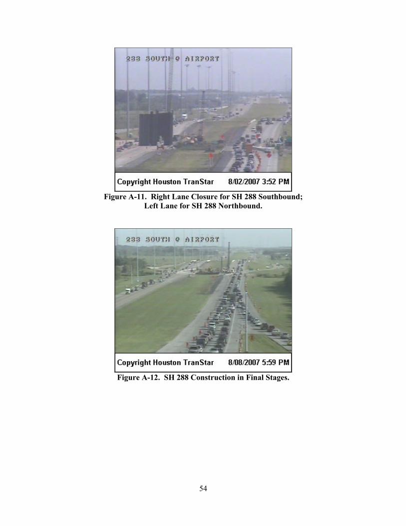
Figure A-11. Right Lane Closure for SH 288 Southbound;

Left Lane for SH 288 Northbound.

Figure A-12. SH 288 Construction in Final Stages.

54

Figure A-13. Street View of SH 288 Northbound Lane Closure.

55

Sites 9 and 10 – IH 35 North of George Beach

• One lane of three-lane roadway closed. • Site 9 for a northbound lane closure. • Site 10 for a southbound lane closure.

Figure A-14. Location of IH 35 Work Zone for Sites 9 and 10.

Figure A-15. Traffic Congestion in IH 35 Work Zone.

56

Site 13 – IH 45 North Freeway Southbound at Little York

• Data collected from manual counts of TranStar CCTV video. • Right lane and shoulder were closed for CCTV camera maintenance. • This was a short-term daytime only single-day closure.

Figure A-16. Work Zone Layout for Site 13.

Figure A-17. TranStar Camera View of Lane Closure.

57

Figure A-18. Traffic Flowing through IH 45 Work Zone.

58

Site 14 – US 290 Eastbound at Gessner

• Night time closure for pavement repair. • Data collected March 20, 2008 from TranStar radar sensor.

Figure A-19. Location of US 290 Eastbound at Gessner Work Zone.

59

Site 15 – US 290 Westbound at Jones Road

• Night time closure for pavement repair. • Data collected May 13 and 14, 2008 by manual field counts. • Significant portion of traffic observed to detour to freeway frontage road.

Figure A-20. Location of US 290 Westbound at Jones Road Nighttime Lane Closure.

60

Figure A-21. TranStar CCTV Image of Lane Closure.

Figure A-22. Traffic Queuing Approaching Lane Closure.

61

Sites 16, 17, 18, and 19 – San Antonio, Texas

Figure A-23. Location of Study Sites in San Antonio.

Site 16 – IH 35 Southbound at Splashtown

• One left lane of three lanes closed. • Data collected using TransGuide sensors. • Closure data for 12:45 pm – 3:00 pm on June 25, 2008.

62

63

Site 17 – IH 410 at San Pedro

• Five-lane section narrowed down to one lane over about a mile. • Data collected over a weekend.

Figure A-24. Traffic Congestion at Site 17.

Site 18 – IH 410 at Rolling Ridge

• No lanes were closed. • Three-lane section with narrow lanes, CTB adjacent to travel lane, and no shoulders.

Figure A-25. TransGuide View of Traffic at Site 18 in San Antonio.

APPENDIX B. SUMMARY OF DATA INPUT FOR MODEL VALIDATION

Table B-1. Input Values of QUEWZ-92. QUEWZ-92 Site

Input 1 2 3 4 5 6 7 8 9 10 11 12 Percentage of Truck 5 5 4 4 4 15 15 11 11 3 6 5

Total Lanes 2 3 3 3 3 2 2 3 3 4 4 3 Open Lanes 1 2 2 2 2 1 1 2 2 3 3 2

Length of Lane Closure 0.5 3.0 0.3 0.3 0.3 1.2 1.2 1.3 1.9 1.5 0.3 1.0 Lane Closure Begins 6 0 0 0 6 9 12 0 9 0 9 0 Lane Closure Ends 14 24 24 24 20 11 14 24 14 24 12 24

Work Activity Begins - 12 - 8 - 9 12 9 9 17 9 7 Work Activity Ends - 16 - 19 - 11 14 16 14 18 12 8

Hourly Volume/ AADT AADT AADT AADT AADT AADT Volume Volume Volume Volume AADT AADT AADTFree Flow Speed 60 60 60 60 60 60 60 60 60 60 60 60 Breakpoint Speed 46 46 46 46 46 46 46 46 46 46 46 46 Speed at Capacity 30 30 30 30 30 30 30 30 30 30 30 30

LOS Breakpoint Speed 1850 1850 1850 1850 1850 1850 1850 1850 1850 1850 1850 1850 Volume at Capacity 2000 2000 2000 2000 2000 2000 2000 2000 2000 2000 2000 2000

Table B-2. Input Values of HCS+.

HCS+ SiteInput 1 2 3 4 5 6 7 8 9 10 11 12

Area Type R U R R R U U U U U U U Class 1 3 1 1 1 3 3 3 3 3 3 3

Posted Speed (mph) 50 50 50 50 50 50 50 50 50 50 50 50 Heavy Vehicle 5 5 4 4 4 15 15 11 11 3 6 5

Number of Lanes 2 2 2 2 2 2 2 2 2 3 3 2 K Factor 0.104 0.097 0.104 0.104 0.104 0.097 0.097 0.097 0.097 0.097 0.097 0.104D Factor 0.55 0.55 0.55 0.55 0.55 0.55 0.55 0.55 0.55 0.55 0.55 0.55

Peak Hour Factor 0.95 0.95 0.95 0.95 0.95 0.95 0.95 0.95 0.95 0.95 0.95 0.95Local Adjustment Factor 0.9 0.98 0.9 0.9 0.9 0.98 0.98 0.98 0.98 0.98 0.98 0.9

Table B-3. Input Values of MicroBENCOST.

MicroBENCOST SiteInput 1 2 3 4 5 6 7 8 9 10 11 12

Area Type R U R R R U U U U U U U Total Lanes 2 3 3 3 3 2 2 3 3 4 4 3 Open Lanes 1 2 2 2 2 1 1 2 2 3 3 2

Work zone Length 0.5 3.0 0.3 0.3 0.3 1.2 1.2 1.3 1.9 1.5 0.3 1.0 Lane Closure Begins 6 0 0 0 6 9 12 0 9 0 9 0 Lane Closure Ends 14 24 24 24 20 11 14 24 14 24 12 24

Heavy Vehicle 5 5 4 4 4 15 15 11 11 3 6 5 Access Control None Full None None None Full Full Full Full Full Full Full

Hourly Volume/ AADT AADT AADT AADT AADT AADT Volume Volume Volume Volume AADT AADT AADTCurvature 0 0 0 0 0 0 0 0 0 0 0 0

Lane Width 12 12 12 12 12 12 12 12 12 12 12 12 Shoulder Width 10 10 10 10 10 10 10 10 10 10 10 10 Design Speed 70 65 70 70 70 65 65 65 65 65 65 65

Capacity 1953 1936 1942 1942 1942 1838 1838 1878 1878 1968 1956 1936

65

66

Table B-4. Input Values of Kim’s Model. Kim’s Model Site

Input 1 2 3 4 5 6 7 8 9 10 11 12 Number of Closed Lanes 1 1 1 1 1 1 1 1 1 1 1 1 Location of Closed Lanes 0 1 0 0 0 0 1 0 0 1 1 1

Percentage of Heavy Vehicles 5 5 4 4 4 15 15 11 11 3 6 5 Lateral Distance 0 0.5 1 1 1 0.5 0.5 0.5 0.5 0 1 0

Work Zone Length 0.5 3.0 0.3 0.3 0.3 1.2 1.2 1.3 1.9 1.5 0.3 1.0 Work Zone Grade 0 0 0 0 0 0 0 0 0 0 0 0

Intensity of Work Activity 0 1 0 1 0 1 1 1 1 1 1 1

APPENDIX C. SUMMARY OF ROAD USER COST MODEL COMPARISON

Table C-1. Updated User Cost Comparison on IH 35 Northbound. Time VISSIM Cost Jiang QUEWZ-92 Cost (hour) Cost ($) Cost (hour) Cost ($)

1 0.043 0.936 0.037 0.811 6.36

2 0.080 1.728 0.050 1.088 4.77

3 0.012 0.251 0.018 0.383 4.77

4 0.032 0.699 0.016 0.346 4.77

5 0.576 12.523 0.544 11.826 12.72

6 0.873 18.955 0.555 12.046 34.98

7 20.089 436.427 20.657 448.759 443.61

8 32.527 706.626 48.090 1044.723 224.19

9 9.605 208.651 9.491 206.189 159

10 9.102 197.731 7.654 166.280 166.95

11 19.628 426.412 18.419 400.149 211.47

12 53.781 1168.349 43.580 946.756 206.7

13 47.158 1024.480 43.086 936.008 213.06

14 49.515 1075.680 35.640 774.251 213.06

15 46.794 1016.559 42.104 914.686 321.18

16 109.624 2381.508 163.800 3558.455 3157.74

17 225.337 4895.300 206.695 4490.305 2593.29

18 95.833 2081.908 89.787 1950.566 143.1

19 50.578 1098.765 42.035 913.176 224.19

20 10.315 224.092 6.213 134.974 149.46

21 3.028 65.772 2.603 56.544 89.04

22 2.741 59.555 2.363 51.328 60.42

23 1.699 36.910 1.273 27.657 44.52

24 0.858 18.643 0.497 10.796 27.03

T-Test 0.944 0.018

RMS Error 280 751

67

68

Table C-2. Updated User Cost Comparison on IH 35 Southbound. Time VISSIM Cost Jiang QUEWZ-92 Cost (hour) Cost ($) Cost (hour) Cost ($)

10 18.06 392.33 18.17 394.82 340.260

11 25.79 560.22 25.81 560.74 248.040

12 36.36 789.91 36.30 788.59 168.540

13 26.68 579.67 26.14 567.88 276.660

14 24.17 525.11 24.28 527.54 337.080

T-Test 0.594 0.035

RMS Error 5.53 350.27

Table C-3. Updated Road User Cost for IH 37 with Left Lane Closure.

Time VISSIM Cost Jiang QUEWZ-92 Cost (hour) Cost ($) Cost (hour) Cost ($) 10 153.17 3460 170.32 3847 3031

11 336.21 7594 341.86 7723 6217

RMS Error 228 1021

Table C-4. Updated Road User Cost for IH 37 with Left Lane Closure.

Time VISSIM Cost Jiang QUEWZ-92 Cost (hour) Cost ($) Cost (hour) Cost ($) 12.5 115.30 2605 94.09 2125 1817

13.5 228.47 5161 208.89 4719 4506

RMS Error 461 724