SANDIA REPORT SAND2013-6768 Unlimited Release Printed August 2013

Capacitor Discharge Pulse Analysis Michael S. Baker, Stewart Griffiths, Danelle M. Tanner Prepared by Sandia National Laboratories Albuquerque, New Mexico 87185 and Livermore, California 94550 Sandia National Laboratories is a multi-program laboratory managed and operated by Sandia Corporation, a wholly owned subsidiary of Lockheed Martin Corporation, for the U.S. Department of Energy's National Nuclear Security Administration under contract DE-AC04-94AL85000. Approved for public release; further dissemination unlimited.

2

Issued by Sandia National Laboratories, operated for the United States Department of Energy by Sandia Corporation. NOTICE: This report was prepared as an account of work sponsored by an agency of the United States Government. Neither the United States Government, nor any agency thereof, nor any of their employees, nor any of their contractors, subcontractors, or their employees, make any warranty, express or implied, or assume any legal liability or responsibility for the accuracy, completeness, or usefulness of any information, apparatus, product, or process disclosed, or represent that its use would not infringe privately owned rights. Reference herein to any specific commercial product, process, or service by trade name, trademark, manufacturer, or otherwise, does not necessarily constitute or imply its endorsement, recommendation, or favoring by the United States Government, any agency thereof, or any of their contractors or subcontractors. The views and opinions expressed herein do not necessarily state or reflect those of the United States Government, any agency thereof, or any of their contractors. Printed in the United States of America. This report has been reproduced directly from the best available copy. Available to DOE and DOE contractors from U.S. Department of Energy Office of Scientific and Technical Information P.O. Box 62 Oak Ridge, TN 37831 Telephone: (865) 576-8401 Facsimile: (865) 576-5728 E-Mail: reports@adonis.osti.gov Online ordering: http://www.osti.gov/bridge Available to the public from U.S. Department of Commerce National Technical Information Service 5285 Port Royal Rd. Springfield, VA 22161 Telephone: (800) 553-6847 Facsimile: (703) 605-6900 E-Mail: orders@ntis.fedworld.gov Online order: http://www.ntis.gov/help/ordermethods.asp?loc=7-4-0#online

3

SAND2013-6768 Unlimited Release

Printed August 2013

Capacitor Discharge Pulse Analysis

Michael S. Baker, Stewart Griffiths, Danelle M. Tanner

Sandia National Laboratories P.O. Box 5800

Albuquerque, NM 87185-1310

Abstract Capacitors used in firing sets and other high discharge current applications are discharge tested to verify performance of the capacitor against the application requirements. Parameters such as capacitance, inductance, rise time, pulse width, peak current and current reversal must be verified to ensure that the capacitor will meet the application needs. This report summarizes an analysis performed on the discharge current data to extract these parameters by fitting a second-order system model to the discharge data and using this fit to determine the resulting performance metrics. Details of the theory and implementation are presented. Using the best-fit second-order system model to extract these metrics results in less sensitivity to noise in the measured data and allows for direct extraction of the total series resistance, inductance, and capacitance.

4

Acknowledgment The authors would like to thank Jeff Lantz for testing and providing feedback on the implementation and use of this code.

5

Table of Contents 1. Introduction ............................................................................................................................. 7 2. Tester operation ...................................................................................................................... 7 3. Analysis Theory ...................................................................................................................... 8

3.1. Over-damped condition .................................................................................................. 10 3.2. Under-damped condition ................................................................................................ 10 3.3. Critically-damped condition ........................................................................................... 11

4. Software Implementation ...................................................................................................... 11 4.1. User Interface and usage guidelines ............................................................................... 12 4.2. Detailed description of software implementation .......................................................... 13

4.2.1. Reading in discharge pulse data .............................................................................. 13 4.2.1.1 _WF Files .............................................................................................................. 14

4.2.1.2 Multi-shot Text File .............................................................................................. 14 4.2.1.3 Single-shot Text File ............................................................................................. 14

4.2.2. Finding the best fit to the data................................................................................. 15 4.2.3. Extracting discharge pulse parameters .................................................................... 19 4.2.4. Saving the results .................................................................................................... 20

5. Conclusions ........................................................................................................................... 21 6. References ............................................................................................................................. 21

List of Figures Figure 2-1: Circuit schematic of discharge life tester. .................................................................... 7

Figure 2-2: Sample discharge current data as measured directly from oscilloscope. ..................... 8 Figure 3-1: Source-free series RLC circuit used in modeling discharge current. ........................... 9 Figure 4-1: Screen capture of software user interface. ................................................................. 12 Figure 4-2: Plot showing the process used to identify the zero offset window. ........................... 16 Figure 4-3: Data with initial fit and data trimming shown. .......................................................... 18 Figure 4-4: Trimmed data shown with final fit. ............................................................................ 19 Figure 4-5: Plot of best-fit discharge curve illustrating extracted parameters. ............................. 20

6

7

1. Introduction Analyzing the current discharge profile versus time for a high voltage capacitor used in firing sets is important in quantifying the capacitor performance and verifying that it meets the application requirements. For example, the current discharge profile is used to measure specifications such as rise time, peak current, pulse width, and current reversal. However, there is an opportunity to use this data to extract even more information about the capacitor under test by fitting a model of a series RLC circuit to the data in order to determine the total series inductance, resistance, and capacitance of the test circuit [1,2]. Using this model fit can also improve the extraction of other parameters by smoothing out the noise that is inherent in this data to allow for a more accurate measure of the capacitor discharge performance. This report will present the theory and operation of a software program used to fit a series RLC circuit model to the discharge data from a variety of different discharge life testers to enable a more complete characterization of the capacitor performance and lifetime.

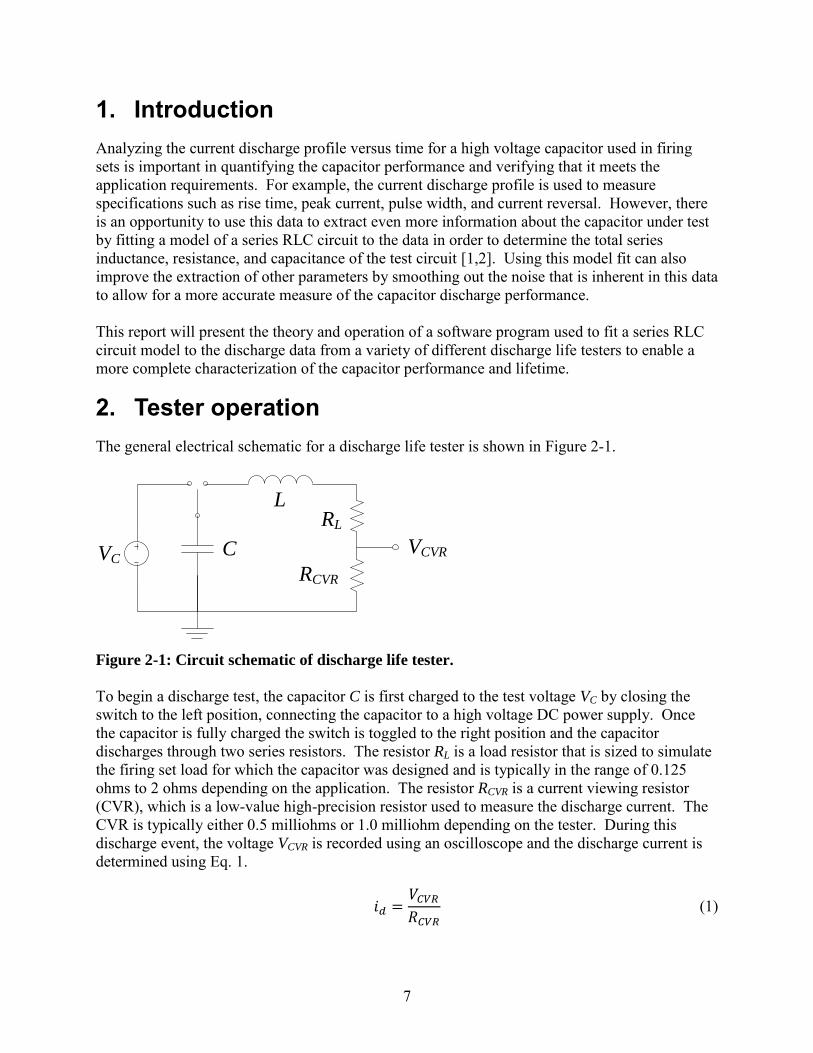
2. Tester operation The general electrical schematic for a discharge life tester is shown in Figure 2-1.

Figure 2-1: Circuit schematic of discharge life tester.

To begin a discharge test, the capacitor C is first charged to the test voltage VC by closing the switch to the left position, connecting the capacitor to a high voltage DC power supply. Once the capacitor is fully charged the switch is toggled to the right position and the capacitor discharges through two series resistors. The resistor RL is a load resistor that is sized to simulate the firing set load for which the capacitor was designed and is typically in the range of 0.125 ohms to 2 ohms depending on the application. The resistor RCVR is a current viewing resistor (CVR), which is a low-value high-precision resistor used to measure the discharge current. The CVR is typically either 0.5 milliohms or 1.0 milliohm depending on the tester. During this discharge event, the voltage VCVR is recorded using an oscilloscope and the discharge current is determined using Eq. 1.

(1)

VC

RCVR

RL

L

C VCVR

8

In the circuit shown in Figure 2-1, the inductor I is a combination of the self-inductance of the wound capacitor and the parasitic inductance created by the tester wiring. It is not purposefully added to the test circuit but is always present to some level based on the tester design and total cable length. There is also some parasitic resistance of the test cables which is lumped together with the load resistor RL. Any parasitic capacitance in the tester would be lumped together with C, the capacitor under test. However, parasitic capacitances are believed to be very small compared to the test capacitor value. An example of the measured current from a discharge event is shown in Figure 2-2. Note that depending on the tester and oscilloscope used, there can be more noise in the signal, and the time duration of data before and after the discharge event can vary substantially based on the trigger settings in the tester. This sample discharge data will be used throughout this report as a case study whenever data processing is discussed.

Figure 2-2: Sample discharge current data as measured directly from oscilloscope.

3. Analysis Theory Once the capacitor is fully charged by the source voltage and the switch is moved into the discharge position the circuit can be modeled as a source-free series RLC circuit as shown in Figure 3-1. The resistor, R, is the sum of the load resistor, RL, and the CVR, RCVR. For the sign convention used in this analysis, when the capacitor voltage is positive and the current is negative the capacitor is discharging.

0 500 1000 1500 2000-1000

-500

0

500

1000

1500

2000

2500Sample Discharge Pulse

Time (nano-seconds)

Cu

rre

nt

(am

ps

)

9

Figure 3-1: Source-free series RLC circuit used in modeling discharge current.

The resulting series RLC circuit is described by a second order differential equation. The derivation of this solution is presented in detail in [3], and will be summarized in this section. This system can be modeled by using Kirchhoff’s voltage law to sum the voltage drop across each circuit element.

(2)

∫

(3)

This becomes a second order differential equation by taking the derivative of Eq. 3 and rearranging terms.

(4)

where

(5)

√ (6)

The term is the un-damped natural frequency, and the term is the damping factor. Assuming an exponential form for the solution, the general solution is given by:

( )

(7)

where

R

L

C i+-

V0

10

√ (8)

√ (9)

The constants A1 and A2 can be solved for by applying the initial conditions. For a discharge test, the initial current is zero and the initial voltage across the capacitor is V0. The zero initial current boundary condition is applied to Eq. 7, with the solution indicating that A1 is equal to the negative of A2. Equation 7 then simplifies to:

( ) ( ) (10)

The second boundary condition is applied to Eq. 3, resulting in the following:

(11)

(12)

By differentiating Eq. 10, and applying the boundary condition given by Eq. 12, the value for the constant A can be found. This results in the general solution:

( )

√ ( ) (13)

3.1. Over-damped condition For the over-damped solution, where is greater than , the general solution is applied directly. By substituting in s1 and s2, this simplifies to the following:

( )

√ (

(√ )

(√ ) ) (14)

3.2. Under-damped condition When the system is under-damped, meaning that is less than , the term under the square root becomes negative, resulting in a complex solution. In the under-damped case, a new parameter d is defined as the damped natural frequency.

11

√ (15)

The roots s1 and s2, and the general solution given by Eq. 13, can then be re-written as:

(16)

(17)

( )

( ) (18)

By applying Euler’s identities, the complex exponents can be re-written as summations of sine and cosine functions. The resulting equation is simplified to the following solution:

( )

( ) (19)

3.3. Critically-damped condition In the case where is equal to , the system is critically damped. This will result in a division by zero for both the over and under-damped solutions. In this case the original assumption of an exponential solution is incorrect. Details of the critically damped solution derivation can be found in [3]. The final general solution for this case is given as:

( ) ( ) (20)

The constants A1 and A2 can be found by applying the initial conditions as described previously. The resulting solution is:

( )

(21)

4. Software Implementation With an understanding of the equation describing the current flow in a capacitor discharge event, it is possible to fit this equation to the measured data from an event to determine values for the series inductance, capacitance, and resistance. This provides an additional metric for evaluation of a capacitor and supplements other independent capacitance measurements, and it allows for verification of the tester total resistance and inductance for comparison against the application requirements. The fit current profile can also be used to extract other metrics of interest in a discharge test, such as peak current, rise time, pulse width, and reversal. These parameters can

12

be extracted from the raw measured data as well, but results can be significantly affected by noise in the data whereas the best-fit solution will be noise-free.

4.1. User Interface and usage guidelines Analysis code has been written using Matlab version 2011a to find the best fit of the discharge equation to measured data and extract other relevant parameters. A screen capture of the user interface for this software is shown in Figure 4-1. At the time of this writing, the most recent version of the software is 1.07 as shown on the graphical interface (GUI) window under the title.

Figure 4-1: Screen capture of software user interface.

There are only a few user inputs required for this analysis, as seen on the graphical user interface.

1. “Save individual data files” – if this box is selected, a .CSV file will be saved for each selected discharge pulse with information on that one discharge event. The file will contain all extracted parameters as well as the time, measured current, and best fit current values. The measured current column in this file has been corrected for zero offset, but has not been trimmed to the number of fit periods (see Section 4.2.2). The file will be saved in the same directory as the selected results file, with the same name as the input data file. The text “_cycleData_##” is appended to the file name, where ## is the cycle number for the test.

2. “Save individual fit curves” – if this box is selected, a .PNG image file will be saved for each cycle showing the original data after zero correction, and the fit curve. Values of the effective series inductance, capacitance, and resistance from the best fit are shown in the figure legend. The file will be saved in the same directory as the results file, with the same name as the input. The text “_cyclePlot_##” is appended to the file name, where ## is the cycle number for the test.

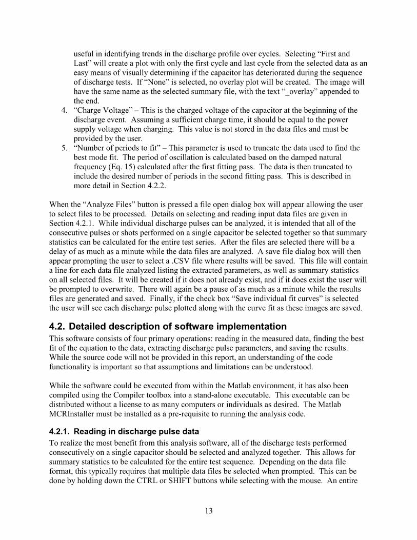
3. “Overlay Plots – This drop down selection box allows the user to select an overlay plot option. Selecting “All” will create a single plot with all cycles plotted together. This is

13

useful in identifying trends in the discharge profile over cycles. Selecting “First and Last” will create a plot with only the first cycle and last cycle from the selected data as an easy means of visually determining if the capacitor has deteriorated during the sequence of discharge tests. If “None” is selected, no overlay plot will be created. The image will have the same name as the selected summary file, with the text “_overlay” appended to the end.

4. “Charge Voltage” – This is the charged voltage of the capacitor at the beginning of the discharge event. Assuming a sufficient charge time, it should be equal to the power supply voltage when charging. This value is not stored in the data files and must be provided by the user.

5. “Number of periods to fit” – This parameter is used to truncate the data used to find the best mode fit. The period of oscillation is calculated based on the damped natural frequency (Eq. 15) calculated after the first fitting pass. The data is then truncated to include the desired number of periods in the second fitting pass. This is described in more detail in Section 4.2.2.

When the “Analyze Files” button is pressed a file open dialog box will appear allowing the user to select files to be processed. Details on selecting and reading input data files are given in Section 4.2.1. While individual discharge pulses can be analyzed, it is intended that all of the consecutive pulses or shots performed on a single capacitor be selected together so that summary statistics can be calculated for the entire test series. After the files are selected there will be a delay of as much as a minute while the data files are analyzed. A save file dialog box will then appear prompting the user to select a .CSV file where results will be saved. This file will contain a line for each data file analyzed listing the extracted parameters, as well as summary statistics on all selected files. It will be created if it does not already exist, and if it does exist the user will be prompted to overwrite. There will again be a pause of as much as a minute while the results files are generated and saved. Finally, if the check box “Save individual fit curves” is selected the user will see each discharge pulse plotted along with the curve fit as these images are saved.

4.2. Detailed description of software implementation This software consists of four primary operations: reading in the measured data, finding the best fit of the equation to the data, extracting discharge pulse parameters, and saving the results. While the source code will not be provided in this report, an understanding of the code functionality is important so that assumptions and limitations can be understood. While the software could be executed from within the Matlab environment, it has also been compiled using the Compiler toolbox into a stand-alone executable. This executable can be distributed without a license to as many computers or individuals as desired. The Matlab MCRInstaller must be installed as a pre-requisite to running the analysis code.

4.2.1. Reading in discharge pulse data To realize the most benefit from this analysis software, all of the discharge tests performed consecutively on a single capacitor should be selected and analyzed together. This allows for summary statistics to be calculated for the entire test sequence. Depending on the data file format, this typically requires that multiple data files be selected when prompted. This can be done by holding down the CTRL or SHIFT buttons while selecting with the mouse. An entire

14

directory of files can be selected by double-clicking on the directory and pressing CTRL-A to select all files in that directory. This software has been designed to work with the output from multiple testers, including the PT3726 product tester as well as several new research testers. Subsequent analysis routines assume that current is in amps and time in nano-seconds, with a positive current indicating a discharge of the capacitor. Any data read from a supported file format using a different set of units or sign convention will be converted to positive discharge current, nano-seconds, and amps when it is read by the software. Supported data file formats are described in the following sections.

4.2.1.1 _WF Files This is a binary file format used by the PT3726 product tester. The file is saved without a file extension, but with the text “_WF” as the final 3 characters of the filename. The file is in the Labview Datalog binary format which is not well documented. Because of the lack of complete documentation of the file format, several assumptions are made while reading this file type so that the resulting data is correctly imported from the PT3726 tester, which is currently the only tester known to use this file format. Specifically, the raw time vector is not saved in the file but is reconstructed based on an assumed time step of 0.2 nanoseconds and a data vector length of 10,000 data points. Any future testers that might use this format must maintain this same time increment and data vector size. The current is stored as double precision floating point values with units of negative amps. The file name must end in “_WF”, and somewhere in the file name the cycle number must be included using the text “Cyc#” followed by the cycle number. For example, “SN1234_Main_Cyc#123_WF” would be valid and would indicate cycle number 123 of the test. The PT3726 automatically adds the “_Cyc#xxx_WF” to the file name.

4.2.1.2 Multi-shot Text File A text file format is supported with all of the data for multiple sequential discharge tests saved in a single file. This file is characterized by a first header line with the exact text “Discharge Pulse Tester Data” followed by six additional header lines, and data in columns for each shot. The first column is the time vector in seconds, and each additional column is the current discharge data for a single shot in negative k-amps. Columns are separated by tabs, and each data column has a header in the last header line that labels the shot number. For example, the seventh line in the file would contain “Time<TAB>Shot 1<TAB>Shot 2<TAB>Shot 3” where <TAB> indicates a tab character. The single file can contain an unlimited number of shots. The current data can have either a positive or negative sign, the software will automatically detect and correct the sign so that the data uses the positive discharge convention.

4.2.1.3 Single-shot Text File A final text file format is supported where only a single shot is saved in each data file. The data is in two columns, separated by a tab character. The first column is the time in seconds and the second column is the current in k-amps. A single optional header line is supported with the text “Discharge Pulse Data (sec. amp)”. This header can have additional text on the same line, but the first 31 characters must be an exact match to this text string. Note that while the header text

15

describes the units as seconds and amps, the file must be saved in seconds and k-amps. The current discharge can have either a positive or a negative sign, the software will automatically detect the sign of the current and reverse it if necessary. The filename should contain the cycle number, using the same format as the multi-shot text file. Some part of the file name should contain the text “_cyc” followed by the cycle number, followed by another underscore. For example, “SN1234_Main_cyc123_.txt” would be a valid name indicating cycle number 123. This should be added to the file name by the tester software.

4.2.2. Finding the best fit to the data The values for R, L, and C of the discharge circuit, as described in Section 3, can be found by determining the best-fit of Eq. 19 to the measured data. Because the data recorded from the tester does not begin precisely at the start of the discharge event, a fourth fitting parameter must also be determined which is the time that the discharge begins, or T0. All curve-fitting is performed using the Matlab lsqnonlin() function in the Optimization toolbox. This function uses a Newton method approach to solve a nonlinear least-squares data-fitting problem by minimizing the sum of the square of the error between the model fit and the data at each point. A starting guess must be provided, and the algorithm iterates on the values of R, L, C, and T0, until the error is minimized. The quality of the starting guess can significantly impact the ability of the algorithm to converge on a solution, so it is important that the starting guess be reasonable. The first step in the fitting process is to ensure that the data is correctly centered at zero. Depending on the tester and oscilloscope settings there have been data sets that include a non-zero offset in the current data. This means that the measurement before the discharge begins is not centered at zero current as it should be. This is an artifact of the data measurement process and does not indicate a real current. To correct this, a window of data before the pulse begins is selected, and the average value of all data points in that window is calculated. This average is then subtracted from all of the data to re-center it on zero. To determine the size of this averaging window the point of max current is identified, as well as the point where the current is at 30% of the max value. These two points are selected without regard to noise in the data, they are found as simply the maximum measured current and the first point with a value greater than 30% of this maximum. From these two points, a line is drawn back to zero and this point is identified as the maximum window size. Then to ensure that the pulse is not improperly truncated due to noise in the data, the averaging window is set to 75% of this maximum window size. Figure 4-2 illustrates this process on the data shown in Figure 2-2, with the averaged data shown in Pink. The calculated offset for this data set is -6.31 amps. Should the measured data not have enough lead-in to identify the averaging window this step will be skipped.

16

Figure 4-2: Plot showing the process used to identify the zero offset window.

At this point, a best-fit optimization could be performed to solve for the values of R, L, C, and T0. However, the ability of the non-linear least-squares fitting algorithm to converge on a solution is dependent on the number of parameters in the fit and the accuracy of the initial starting guesses for the fit parameters. With four parameters, and no guidance on their starting values, the algorithm will often fail to converge. To improve the robustness of this process, some additional information can be determined from the data. After the data has been adjusted for zero offset, a first-pass estimate of the capacitance is determined by integrating the current over time using the following equation.

∫

(22)

It is important to perform the zero offset correction before this integration or any error in offset will be integrated into an error in the capacitance estimate. Also, error will be introduced into this estimate if the data does not capture the complete discharge event, such that the current has not returned to zero by the end of the measured data. For the sample data from Figure 2-2, the integrated capacitance is 60.5 nF. A first-pass fit of the model to the data is then performed, where the capacitance is not included as a fitting term, but is held constant at the estimated value based on the integral of the current.

0 500 1000 1500 2000-1000

-500

0

500

1000

1500

2000

2500Zero Offset Calculation

Time (nano-seconds)

Cu

rre

nt

(am

ps

)

Max Current

30% of MaxCurrent

Maximum window sizefrom extrapolation

ZeroOffsetAveragingWindow

17

The initial starting guess for T0 is set to the time at the point where the current is at 30% of the max current, as shown in Figure 4-2. This estimate is slightly higher than the true value of T0, but serves as a good starting guess for the fitting algorithm. With no other information to guide the decision, the starting guess for resistance defaults to 0.9 ohms, and the default inductance starting guess is 50 nH. These starting guesses were set based on previously measured nominal values. The fitting algorithm may not properly converge if a tested resistance and inductance differ significantly from these values. Using the integrated capacitance to eliminate this term from the fit has been found to improve the ability of the algorithm to converge over various test cases by reducing the number of free parameters in the fit. The initial fit provides a very good estimate for all of the fitting parameters. The values for R, L, and C are used to estimate the damped natural frequency of the second order system using Eq. 15, and this is used to determine the period of oscillation as:

√

(23)

The measured data is then trimmed to the range of T0 – P/8 to T0 + nP, where n is the number of periods to fit as input by the user on the graphical interface. Using the default value of 2 for n, the sample data in Figure 2-2 is shown with the first-pass curve fit in red and the trimmed data indicated in pink. The original data has also been adjusted to remove any zero offset. The calculated values for R, L, C, T0, and P are shown in the figure legend. Note that the value for C was not determined in the fit but was held fixed at the integrated value. It is possible to have a discharge test that is over-damped so that the period of oscillation is undefined. In this case, the analysis routine does not trim the data and the second curve fit is performed across the entire data range. Otherwise, this analysis works equally well with over- or under-damped systems.

18

Figure 4-3: Data with initial fit and data trimming shown.

The quality of fit for this first pass is relatively good. However, it can be improved by using the fit parameters from the first fit as the starting values for a second-pass curve-fit. In this second pass, the data used in the fit will be trimmed based on the number of periods selected in the GUI as discussed in the previous paragraph. Also, the capacitance will be a free term in the fitting process instead of being held fixed at the value found by integration. Trimming the data causes the result to be less sensitive to noise in the beginning and end of the data after the current discharge has completed. The final fit is shown in the following figure, with only the trimmed data shown. Values for L, C, and R are shown in the figure legend, and have only changed slightly from the first-pass fit values. The quality of this fit can be measured by reporting the average of the absolute value of the difference between each data point and curve-fit value. For this example, the average fit error is 25.9 amps after the second pass fit. A second metric used to assess the quality of the analysis routine is to compare the final capacitance determined from curve fitting with the integrated capacitance. In this case the difference is only 3.1 nF. Very large values for either of these two metrics would indicate a problem with the curve fit or with the data.

0 500 1000 1500 2000-1000

-500

0

500

1000

1500

2000

2500Initial Fit Results and Data Trimming

Time (nano-seconds)

Cu

rre

nt

(am

ps

)

L= 49.0 nHC= 60.5 nFR= 0.809 ohmT0= 700.9 nsP=382.9 ns

Initial fit (red)

Truncatedfor final fit

Truncatedfor final fit

19

Figure 4-4: Trimmed data shown with final fit.

4.2.3. Extracting discharge pulse parameters In addition to the series resistance, inductance and capacitance of the discharge circuit, several other metrics are of interest in characterizing the discharge pulse. A list of these parameters, and a description of how they are determined, is provided below.

Peak current - This is found by first identifying the maximum positive value of current. A second order polynomial curve fit is then found for the maximum point and the point before and after the max. The peak can then be found as the maximum of the second order polynomial, or the point in the polynomial with a zero slope.

Time at peak current – Found from the polynomial fit solution as described above. This time is given relative to the original full data set, not the final trimmed data.

Max current reversal – First, the maximum negative current is found using the same technique that is used to find peak current. Then the current reversal is defined as the absolute value of the ratio of the peak negative current divided by the peak positive current.

Time at max reversal – Found from the polynomial fit solution for max current reversal. Rise time – The rise time is defined as the time at 90% of the peak current minus the time

at 10% of the peak current on the rising edge of the discharge pulse. Linear interpolation is used to precisely determine the 10% and 90% times based on the two nearest data points that bracket the target current value.

0 200 400 600 800-1000

-500

0

500

1000

1500

2000

2500Final Fit Results

Time (nano-seconds)

Cu

rre

nt

(am

ps

)

Final fit (red)

L= 51.1 nHC= 57.4 nFR= 0.809 ohm

20

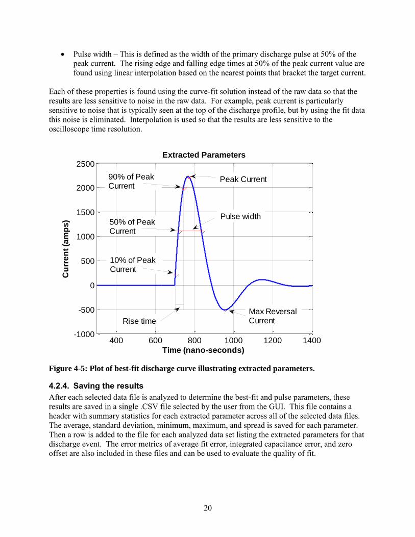
Pulse width – This is defined as the width of the primary discharge pulse at 50% of the peak current. The rising edge and falling edge times at 50% of the peak current value are found using linear interpolation based on the nearest points that bracket the target current.

Each of these properties is found using the curve-fit solution instead of the raw data so that the results are less sensitive to noise in the raw data. For example, peak current is particularly sensitive to noise that is typically seen at the top of the discharge profile, but by using the fit data this noise is eliminated. Interpolation is used so that the results are less sensitive to the oscilloscope time resolution.

Figure 4-5: Plot of best-fit discharge curve illustrating extracted parameters.

4.2.4. Saving the results After each selected data file is analyzed to determine the best-fit and pulse parameters, these results are saved in a single .CSV file selected by the user from the GUI. This file contains a header with summary statistics for each extracted parameter across all of the selected data files. The average, standard deviation, minimum, maximum, and spread is saved for each parameter. Then a row is added to the file for each analyzed data set listing the extracted parameters for that discharge event. The error metrics of average fit error, integrated capacitance error, and zero offset are also included in these files and can be used to evaluate the quality of fit.

400 600 800 1000 1200 1400-1000

-500

0

500

1000

1500

2000

2500Extracted Parameters

Time (nano-seconds)

Cu

rre

nt

(am

ps

)

Max ReversalCurrent

10% of PeakCurrent

50% of PeakCurrent

90% of PeakCurrent

Peak Current

Pulse width

Rise time

21

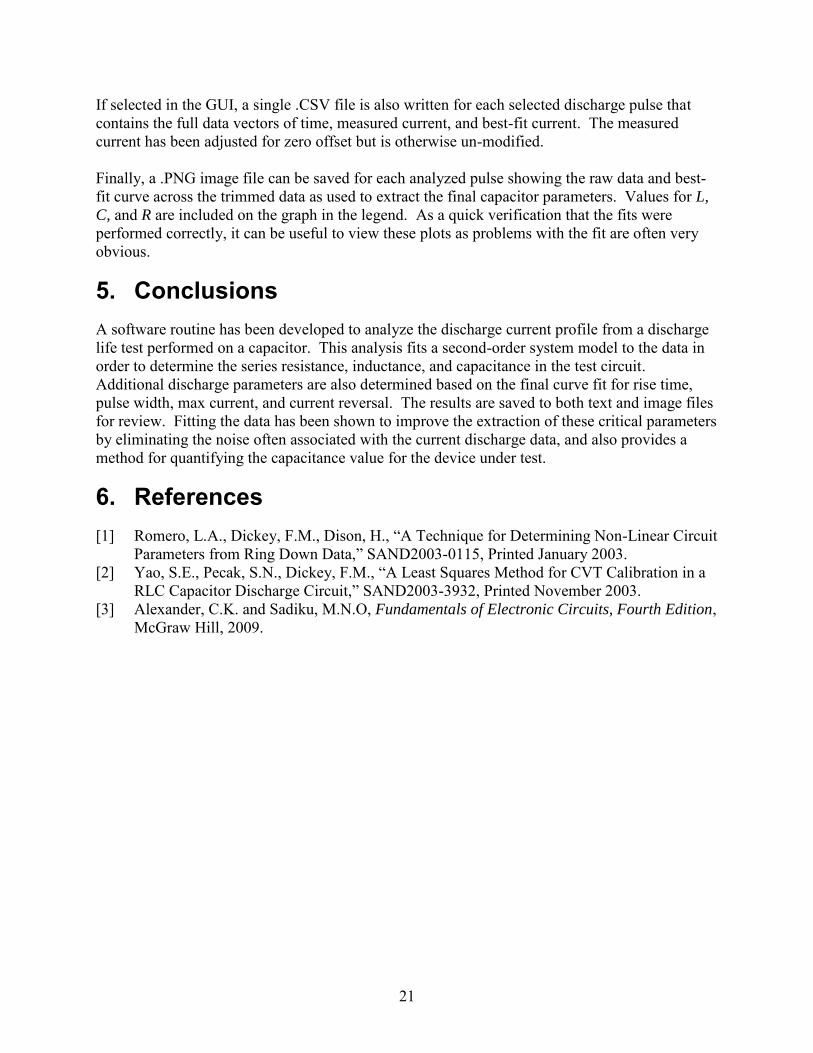
If selected in the GUI, a single .CSV file is also written for each selected discharge pulse that contains the full data vectors of time, measured current, and best-fit current. The measured current has been adjusted for zero offset but is otherwise un-modified. Finally, a .PNG image file can be saved for each analyzed pulse showing the raw data and best-fit curve across the trimmed data as used to extract the final capacitor parameters. Values for L,

C, and R are included on the graph in the legend. As a quick verification that the fits were performed correctly, it can be useful to view these plots as problems with the fit are often very obvious.

5. Conclusions A software routine has been developed to analyze the discharge current profile from a discharge life test performed on a capacitor. This analysis fits a second-order system model to the data in order to determine the series resistance, inductance, and capacitance in the test circuit. Additional discharge parameters are also determined based on the final curve fit for rise time, pulse width, max current, and current reversal. The results are saved to both text and image files for review. Fitting the data has been shown to improve the extraction of these critical parameters by eliminating the noise often associated with the current discharge data, and also provides a method for quantifying the capacitance value for the device under test.

6. References [1] Romero, L.A., Dickey, F.M., Dison, H., “A Technique for Determining Non-Linear Circuit

Parameters from Ring Down Data,” SAND2003-0115, Printed January 2003. [2] Yao, S.E., Pecak, S.N., Dickey, F.M., “A Least Squares Method for CVT Calibration in a

RLC Capacitor Discharge Circuit,” SAND2003-3932, Printed November 2003. [3] Alexander, C.K. and Sadiku, M.N.O, Fundamentals of Electronic Circuits, Fourth Edition,

McGraw Hill, 2009.

22

Distribution List – Electronic copy only Copies Mail Stop Recipient Organization

1 0525 Danelle Tanner 1732 1 0525 Mark Braithwaite 1732 1 0525 Lauren Cleavall 1732 1 0525 Gregory Frye-Mason 1732 1 0525 Adam Lester 1732 1 0525 Ted Parson 1732 1 0525 Lucas Shiver 1732 1 0525 William Wilbanks 1732 1 0525 David Lee Williams 1732 1 0525 Luke Wyatt 1732 1 0525 Patrick A. Smith 1732 1 0525 Mark Platzbecker 1732 1 0965 Edward Binasiewicz 1732 1 1310 Michael Baker 1719 1 0899 Technical Library 9536