Chapter 5

3D Theory of Thermoelasticity We consider a 3D continuum body that in the 3D cartesian space (O, x, y, z) is occupying at the initial time to a reference configuration C0. In a continuum body there is a one to one correspondence between the material portion of the body and the geometric point of the frame reference. We aim at studying the mechanical response of this body subjected not only to external forces per unit volume x(x, y, z, t) on C0, to extend forces per unit surface f (x, y, z, t) on part of the boundary of 𝐶"    𝜕𝐶" and to assigned displacement u(x, y, z, t) on 𝜕𝐶" but also to a field of temperature variation ΔT (x, y, z, t) with respect to the original temperature T0 (x, y, z, t), being ΔT(x, y, z, t) = T (x, y, z, t) - T0(x, y, z, t). We formulate the general assumption that the temperature variation ΔT (x, y, z, t) is an assigned function of the position and the time, that is that the mechanical behavior is not influencing the temperature distribution that can be determined based on the solution of 3D Fourier equation of heat conduction in solids. This hypothesis is largely adopted in the analysis of thermoelastic problem but not valid in general. In fact for instance in the presence of non conservative constitutive behavior of the material, heat can be generated from the mechanical behavior and the mechanical equation could have an influence, as in other cases as well, in the determination of the temperature fields. On the contrary we assume, as allowed by the physics of the phenomena in most applicative cases, that the mechanical behavior in the presence of thermal action is coupled "in cascade" to the problem of heat conduction. This means, from the modeling viewpoint, that the temperature fields are obtained from the solution of the Fourier equation and are considered for the thermoelastic problem as an additional external action. The state variables describing the mechanical response of a deformable body are the displacement, the strain and the stress. We now define these variables for the 3D continuum and obtain as well the governing equations of the thermoelastic problem for the case of a material that is behaving, as to its mechanical constitutive behavior, as a linear elastic medium.

5.1 Analysis of the deformation

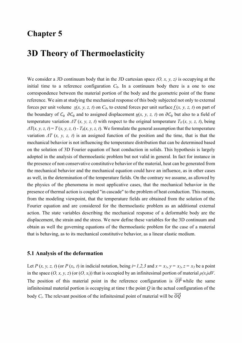
Let P (x, y, z, t) (or P (xi, t) in indicial notation, being i=1,2,3 and x = x1, y = x2, z = x3 be a point in the space (O, x, y, z) (or (O, xi)) that is occupied by an infinitesimal portion of material ρ(xi)dV. The position of this material point in the reference configuration is 𝑂𝑃  while the same infinitesimal material portion is occupying at time t the point Q in the actual configuration of the body Ct. The relevant position of the infinitesimal point of material will be 𝑂𝑄

Figure 5.1: The undeformed and the actual configuration of the body

We define displacement of the continuum body the vector field 𝑃𝑄 = 𝑂𝑄 − 𝑂𝑃  representing the difference of positions occupied by the points of the body at the actual configuration Ct at the time t with respect to the reference configuration. We assume that the generic infinitesimal material portion of the body is identified by the coordinates assumed in the reference configuration. In this case the components of the displacement vector 𝑃𝑄 in the assumed coordinate systems are

( , , , ) ( , , , )( , , , ) ( , , , )( , , , ) ( , , , )

t

t

t

u x y z t x x y z t xv x y z t y x y z t yw x y z t z x y z t z

= −= −= −

(5.1)

or, in indicial notation,

( , ) ( , )ti i i i iu x t x x t x= − (5.2)

This description is usually defined as "lagrangian" approach. In order to avoid separation or "compenetration" of material the function

( , )t ti i ix x x t= (5.3)

has to be continuous and derivable and the Jacobian

ti

j

xJx∂=∂

(5.4)

has be different from zero.

The first state variable of the thermoelastic problem, that is the displacement has now been described. In the definition of the strain variables we are interested to measure, in a pointwise

z

y

x

P

O

Q

C0

C1

manner, the deformation of the body, that is the violation of the rigidity constraint. For a rigid body, any two material points belonging to the body, do not vary their distance during the displacement of the body under some external action.

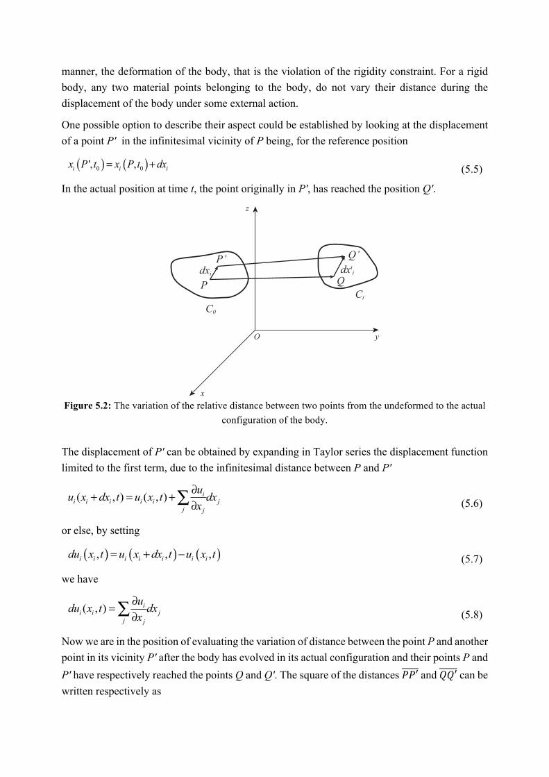
One possible option to describe their aspect could be established by looking at the displacement of a point P' in the infinitesimal vicinity of P being, for the reference position

( ) ( )0 0', ,i i ix P t x P t dx= + (5.5)

In the actual position at time t, the point originally in P', has reached the position Q'.

Figure 5.2: The variation of the relative distance between two points from the undeformed to the actual

configuration of the body.

The displacement of P' can be obtained by expanding in Taylor series the displacement function limited to the first term, due to the infinitesimal distance between P and P'

( , ) ( , ) ii i i i i j

j j

uu x dx t u x t dxx∂+ = +∂∑ (5.6)

or else, by setting

( ) ( ) ( ), , ,i i i i i i idu x t u x dx t u x t= + − (5.7)

we have

( , ) ii i j

j j

udu x t dxx∂=∂∑ (5.8)

Now we are in the position of evaluating the variation of distance between the point P and another point in its vicinity P' after the body has evolved in its actual configuration and their points P and P' have respectively reached the points Q and Q'. The square of the distances 𝑃𝑃′  and 𝑄𝑄′  can be written respectively as

z

y

x

P

O

C0Ct

P’

Q

Q’dxtidxi

2

2

( 1,2,3)

( ) ( 1,2,3)i i

t t ti i

ds dx dx i

ds dx dx i

= =

= = (5.9)

(5.10)

where we assumed that a repeated pedix expressed a summation of the terms, that is

32 2 21 2 3i i i i

idx dx dx dx dx dx dx= = + +∑ (5.11)

By differentiation of eq. 5.2 we have

ti i idu dx dx= − (5.12)

and from eq. 5.8 and eq. 5.12

𝑑𝑥-. = 𝑑𝑥- + 𝑑𝑢- = 𝑑𝑥- +𝜕𝑢-𝜕𝑥11

𝑑𝑥1 (5.13)

so that, from eq. 5.10

2

2( )

( 2

t ii j

j j

i i ii i i j j k

j j kj j k

uds dx dxx

u u udx dx dx dx dx dxx x x

⎛ ⎞∂= + =⎜ ⎟⎜ ⎟∂⎝ ⎠∂ ∂ ∂= + +∂ ∂ ∂

∑

∑ ∑ ∑ (5.14)

where the repeated pedix of the second monomial has been changed with no alteration of the value of the term. Now it is possible to evaluate the square of the variation of distances

𝑑𝑠. 3 − 𝑑𝑠3 = 2𝜕𝑢-𝜕𝑥11

𝑑𝑥-𝑑𝑥1 +𝜕𝑢-𝜕𝑥15

𝜕𝑢-𝜕𝑥51

𝑑𝑥1𝑑𝑥5 (5.15)

or else

𝑑𝑠. 3 − 𝑑𝑠3 = 2𝜕𝑢-𝜕𝑥11

𝑑𝑥-𝑑𝑥1 +𝜕𝑢5𝜕𝑥-1

𝜕𝑢5𝜕𝑥1-

𝑑𝑥-𝑑𝑥1 (5.16)

by setting in the second term appear dxidxj (a similar change in the repeated pedix, as done in the above passage)

𝑑𝑠. 3 − 𝑑𝑠3 = 2 𝑢-,1 +12𝑢5,1𝑢5,- 𝑑𝑥-𝑑𝑥1 (5.17)

where for the indicial notation we assume

,( ) ( ) jjx

∂ ⋅ = ⋅∂

(5.18)

Moreover, assuming that

( ), , , , ,1 1 12 2 2i j i j i j i j j i i j i j j i i ju dx dx u dx dx u dx dx u u dx dx= + = + (5.19)

we can express the variation of the distance in the neighbourhood 2 2( )tds ds− as

2 2( ) 2tij i jds ds dx dxε− = (5.20)

with

( ), , , ,12ij i j j i k i k ju u u uε = + + (5.21)

are the components of the strain vector of Green Lagrange, that expresses the variation of distance between the point P and the point Q in its vicinity, as the configuration of the body evolves from C0 to Ct: this is the pointwise measure of deformation we were looking for.

( , )ij ij ix tε ε= represents a second order tensor.

Figure 5.3: The displacement field in a 1D case.

In case the derivatives ui,j are small with respect to the unity (small displacement gradient), the second term in the expression of the strains, i.e. the nonlinear term, can be neglected. The expression of strain limited to the linear part is then

( ), ,12ij i j j iu uε = + (5.22)

The six above equations (it is easy to recognize that 𝜀-1 = 𝜀1-) are the first ones of the set of governing equations of the thermoelastic problem.

If we express the strain components in terms of the coordinates (x, y, z) instead of xi and the displacement as (u, v, w) instead of ui , we obtain for the first two equations i=1 , j=1,2

12

12

xx

xy

u u ux x xu vy x

ε

ε

∂ ∂ ∂⎛ ⎞= + =⎜ ⎟∂ ∂ ∂⎝ ⎠⎛ ⎞∂ ∂= +⎜ ⎟∂ ∂⎝ ⎠

(5.23)

x,uP P’ Q Q’

du

dx

uu dxx∂+∂

the other form equation can be obtained by rotation of indexes. These components have a physical meaning. If we consider in P an infinitesimal cubic element we can distinguish the point P and P' at the infinitesimal distance dx. Moving from P to P' the displacement has varied of 𝑑𝑢 =9:9;𝑑𝑥,  so the element in the actual configuration has increased its length of du.

𝜀;; is the increase of length per unit length.

Figure 5.4: Change in the relative orientation between two initially orthogonal material segments in the

body.

Similarly, we can consider the same element and the evolution of displacements form C0 to C1 for the points P’ and P’’ at, respectively, a distance dx and dy. Mainly we first consider the variation of the component displacement v of P' along y direction

𝑃′𝑄′ ≃𝜕𝑣𝜕𝑥 𝑑𝑥 = 𝑡𝑎𝑛 𝛼 𝑑𝑥 ≃ 𝛼𝑑𝑥         ⟹        𝛼 ≃

𝜕𝑣𝜕𝑥 (5.24)

and the variation of the displacement component u of P’’ along x direction

𝑃′′𝑄′′ ≃𝜕𝑢𝜕𝑦 𝑑𝑦 = 𝑡𝑎𝑛 𝛽 𝑑𝑦 ≃ 𝛽𝑑𝑦         ⟹        𝛽 ≃

𝜕𝑢𝜕𝑦 (5.25)

that is

( )12xyε α β= + (5.26)

being α + β = γ the variation of the angle between two material segments that were orthogonal in the configuration C0. γ is called the engineering shear strain.

Whereas, by assuming a continuous and derivable set of function ui(xi ,t), it is always possible to obtain by differentiation the expression of 𝜀-1 from the expression of ui , the opposite is not true, that is it is not always possible to obtain a continuous solution of ui(xi ,t) corresponding to a given

expression of 𝜀-1 = 𝜀-1 𝑥-  , 𝑡 . In fact, in the last case the expression of 𝜀-1can be viewed as a set of differential equations of unknown variables ui that can be integrated only if certain conditions are respected. These equations are called compatibility conditions. For monoconnected bodies the 6 equations of compatibility can be expanded as follows

2 22

2 2

2

2

yy xyxx

yz xyxx xz

y x x y

y z x x y z

ε γε

γ γε γ

∂ ∂∂ + =∂ ∂ ∂ ∂

∂ ∂⎛ ⎞∂ ∂∂= − + +⎜ ⎟∂ ∂ ∂ ∂ ∂ ∂⎝ ⎠

(5.27)

(5.28)

The remaining 4 equations can be obtained for rotation of indices. In case of higher order of connectivity additional conditions need to be added.

Anticipating some considerations concerning the constitutive relation, we can attribute to the compatibility equations a special meaning for the 3D thermoelastic problem. In fact, by dealing with 1D models, namely the straight element of a bar exposed to a temperature variation along its axis, it has been established that, in absence of external constraint, no matter what was the temperature variation expression along the axis, no stress was generated in the structure. This result, true for the above particular problem along with its assumptions, is not true in general for 3D continua. In order words it is possible to have a stress field in a free body under the action of a generic temperature variation field ΔT(xi ,t). In fact, let us assume that the strain 𝜀-1 is generated by superimposing the effects of the stress and the temperature, that is the strain is made of a mechanical 𝜀-1Eand a thermal 𝜀-1F component

M Tij ij ijε ε ε= + (5.29)

Let us now assume that, for a temperature variation ΔT, no stress is generated, that is 𝜀-1E = 0. At this point the strain are equal to the thermal strain, that are given, for an isotropic body as

Tij ij Tε δ α= Δ (5.30)

being δij the Kronecker delta with δij = 0 for i ≠ j and δij = 1 for i = j. At this point, if a continuum solution for a displacement is assumed, the no stress solution can be found only if the strain function

( , )ij ij iT x tε αδ= Δ (5.31)

is respecting the compatibility condition. For the presence of derivatives of second order only a linear distribution of ΔT with respect to xi will identically satisfy the compatibility conditions. In other words for linear variation of ΔT (as observed in 1D Fourier's equation closed form solution for the stationary terms) no stress field is generated. In fact, from a particular viewpoint, one can also imagine to ideally divide the continuum in many small parts, as in the grid of the figure below,

Figure 5.5: The continuum body divided into elemental parts.

and allow the elemental parts to expand or contract according to the value of temperature different form one point to another (and maybe also accounting for an anisotropic material behavior). No continuity among these parts can be observed at the end of process. The presence of a stress field and of a relevant mechanical strain component, will give again continuity to the displacement field and will produce for the total strain the satisfaction of the compatibility conditions.

We take, as example, a distribution of ΔT with the form:

𝛥𝑇 𝑥, 𝑦 = 𝑐" + 𝑐K𝑥 + 𝑐3𝑦 + 𝑐L𝑥3 + 𝑐M𝑦3 + 𝑐N𝑥𝑦

𝜀;; = 𝛼𝛥𝑇 𝑥, 𝑦𝜀OO = 𝛼𝛥𝑇 𝑥, 𝑦

𝜀;O = 0

𝜕𝜀;;𝜕𝑦 = 𝛼 𝑐3 + 2𝑐M𝑦 + 𝑐N𝑥  

𝜕3𝜀;;𝜕𝑦3 = 2𝛼𝑐M  

𝜕𝜀OO𝜕𝑥 = 𝛼 𝑐K + 2𝑐L𝑦 + 𝑐N𝑦  

𝜕3𝜀OO𝜕𝑥3 = 2𝛼𝑐L  

 

By substitution in eq. 5.27 we obtain:

z

xO

2𝛼𝑐M + 2𝛼𝑐L = 0

Such equation is verified for certain values of 𝑐L and 𝑐M only. If we use a linear distribution of ΔT respect to x and y, instead of a quadratic one, then the compatibility conditions are always satisfied: no thermal stresses are generated.

5.2 Analysis of tension

We now need to establish how to describe the equilibrium conditions for the deformable body and to identify the state variables that represent the internal strain of the body. We assume that, for the 3D body the laws of Newtonian mechanics are valid, established for a dimensionless material point of mass m that evolves in its position x(t), under the action of an external resultant force f. We assume that a deformable body is in equilibrium if it is in equilibrium each one of its parts. In order to describe the equilibrium of one of the parts of the body it is necessary to describe the internal forces that two parts of the body exchange between each other. We assume that the two parts exchange forces that have the nature of contact forces. We aim at describing the internal state of stress at the generic point P(xi) at the generic time t. Let us image to identify two parts of the body by making a section with a plane passing by P

Figure 5.6: The continuum body divided into two parts by the π plane.

We assume that the part B of the body is applying to the part A a distribution of contact action acting along the plane π. If we imagine a portion of the surface ΔS on the plane π that includes P, it is possible to evaluate the resultant force and moment F and M the distribution of internal action that B is acting on A. In order to define an internal force described at the point P we might evaluate the ratio between F and M with respect to ΔS, let ΔS tend to zero and assume

z

y

x

A

O

B∆S

P

F

M∏

0

0

lim

lim 0

nS

S

F tSMS

Δ →

Δ →

=Δ

=Δ

(5.32)

Being tn the stress vector acting in P on the A part of the body by the B part. The existence of a distribution of internal forces per unit surface can be assumed to be present for each point P and each surface of outer normal n at P. In this way an internal strain vector is defined but, since an infinite number of planes is passing at P, an infinite number of strain vector can be in principle defined at P. Cauchy has demonstrated that once the stress vector is known on three perpendicular planes passing at P, it is also known on any plane of normal n passing through P. In fact we consider an infinitesimal portion of material dm in the neighborhood of P limited by the surfaces A1, A2 and A3 respectively of normal x1, x2 and x3 and dAn of normal n as depicted in figure.

Figure 5.7: The Cauchy tetrahedron.

If we enforce the second law of Newton to this infinitesimal part of the body under the action of the internal forces t(1), t(2), t(3) and t(n) the external body force X (that might include the inertial term as well) we obtain

( )(1) (2) (3) ( )1 2 3 0n

nt dA t dA t dA t dA XdV− + + + + = (5.33)

where the last term can be disregarded since it in an infinitesimal term of higher order with respect to the other ones. By then dividing by dAn and assuming that

P

x1

x3

x2

dA1dA3

dA2

dAn

3t

1t

2t

nt

n

𝐴- = 𝑑𝐴Q𝑐𝑜𝑠 𝑛𝑥S (5.34)

we finally obtain

( ) (1) (2) (3)1 2 3

nt t n t n t n= + + (5.35)

 

Figure 5.8: Stresses decomposition.

where 𝑛- = 𝑐𝑜𝑠 𝑛𝑥S , or else, assuming ( )1 2 3

ii i it i j kσ σ σ= + + , σij is the xj component of the

stress vector acting on the surface of normal xi. Once the nine components σij are known, it is also known the stress vector on the surface with normal n of components ti

(n).

ni ij jt nσ= (5.36)

Since σij relates two vectors (tensors of the first order) they represents the components of a second order tensor in the 3D space. The equilibrium equation can now be derived. For sake of simplicity and for obtaining a more intuitive insight on the role played by the components of the stress term σij we consider the equilibrium of a 3D parallelepiped infinitesimal body in the neighborhood of P of length dx1, dx2 and dx3.

Figure 5.9: Infinitesimal part of the continuum.

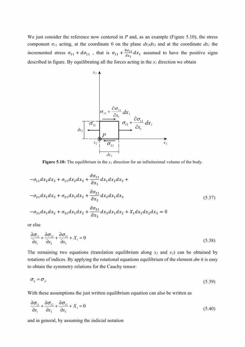
We just consider the reference now centered in P and, as an example (Figure 5.10), the stress component σ11 acting, at the coordinate 0 on the plane dx2dx3 and at the coordinate dx1 the

incremented stress 𝜎KK + 𝑑𝜎KK , that is 𝜎KK +9UVV9;V

𝑑𝑥K assumed to have the positive signs

described in figure. By equilibrating all the forces acting in the x1 direction we obtain

Figure 5.10: The equilibrium in the x1 direction for an infinitesimal volume of the body.

−𝜎KK𝑑𝑥3𝑑𝑥L + 𝜎KK𝑑𝑥3𝑑𝑥L +𝜕𝜎KK𝜕𝑥K

𝑑𝑥K𝑑𝑥3𝑑𝑥L +

−𝜎3K𝑑𝑥K𝑑𝑥L + 𝜎3K𝑑𝑥K𝑑𝑥L +𝜕𝜎3K𝜕𝑥3

𝑑𝑥3𝑑𝑥K𝑑𝑥L

−𝜎LK𝑑𝑥K𝑑𝑥3 + 𝜎LK𝑑𝑥K𝑑𝑥3 +𝜕𝜎LK𝜕𝑥L

𝑑𝑥L𝑑𝑥K𝑑𝑥3 + 𝑋K𝑑𝑥K𝑑𝑥3𝑑𝑥L = 0

(5.37)

or else

3111 211

1 2 3

0Xx x x

σσ σ ∂∂ ∂+ + + =∂ ∂ ∂

(5.38)

The remaining two equations (translation equilibrium along x2 and x3) can be obtained by rotations of indices. By applying the rotational equations equilibrium of the element dm it is easy to obtain the symmetry relations for the Cauchy tensor:

ij jiσ σ= (5.39)

With these assumptions the just written equilibrium equation can also be written as

1311 121

1 2 3

0Xx x x

σσ σ ∂∂ ∂+ + + =∂ ∂ ∂

(5.40)

and in general, by assuming the indicial notation

, 0 , 1,2,3.ij j iX i jσ + = = (5.41)

At the points on the boundary Sf of normal n of the volume V, where the external forces per unit surface fi are applied, by using the same considerations of the Cauchy tetrahedron we obtain

ij i in fσ = (5.42)

5.3 Constitutive Relations

Thermoelasticity constitutive relations in 3D are based on the superposition of effect of the mechanical strain 𝜀-1E, that is the strain caused by the stress field, and the thermal strain 𝜀-1F , caused by the variation of the temperature ΔT from its original value. The total strain 𝜀-1 can then be written as

M Tij ij ijε ε ε= + (5.43)

In the mechanical response of solids and structures subjected to thermal variation, the thermal strain can be expressed as

Txx xTyy y

Tzz z

T

T

T

ε αε α

ε α

= Δ

= Δ

= Δ

(5.44)

with

0T T Txy yz zxε ε ε= = = (5.45)

accounting for some degree of anisotropy, namely the ortotropy of the material, that allows the thermal expansion coefficient to be different in the three directions x, y, z while accounting for the symmetry just with respect to the axes x, y and z. In general we might assume for the thermal expansion an expression of the kind

Tij ij Tε α= Δ (5.46)

The expression shows the tensorial nature of the thermal expansion that represent a linear operator that links a scalar, the temperature variation, to a second order tensor, the strain, 𝛼-1 being a second order tensor as well. This is important, for the special case of anisotropy just mentioned before, to obtain the components of the thermal expansion tensor 𝜀XQ measured in another frame of reference (O, xm , xn , xk) in terms of the components 𝜀-1 measured in (O, x1 , x2 , x3)

mn i j ijm nε ε= (5.47)

with 𝑚- = 𝑐𝑜𝑠 𝑚𝑥S and 𝑛- = 𝑐𝑜𝑠 𝑛𝑥S . The thermal expansion coefficient is in general

dependent upon the temperature level 𝛼-1 = 𝛼-1 𝑇 . This circumstance induces a factor of non

linearity to the mathematical model of the thermoelastic response. As to the mechanical strain, in the thermoelastic problem it is assumed that the linear elastic generalized Hooke law is valid, but in general the elastic components need to be considered dependent upon temperature as well. This is also true for the level of strength of the considered for the yield and the ultimate failure, that, obvious, are dependent upon temperature as well.

In the isotropic case the components of strain can be expressed in terms of the stress components as follows

𝜀;;E =1𝐸 𝜎;; −

𝜈𝐸 𝜎OO −

𝜈𝐸 𝜎\\

𝜀OOE = −𝜈𝐸 𝜎;; +

𝜈1𝐸 𝜎OO −

𝜈𝐸 𝜎\\

𝜀\\E = −𝜈𝐸 𝜎;; −

𝜈𝐸 𝜎OO +

1𝐸 𝜎\\

𝜀O\E =12 𝛾O\ =

12𝐺 𝜎O\

𝜀\;E =12 𝛾\; =

12𝐺 𝜎\;

𝜀;OE =12 𝛾;O =

12𝐺 𝜎;O

(5.48)

with 2(1 )EGν

=+

being the shear elastic constant, 𝜈 the Poisson's coefficient and E the Young's

modulus. The shear components 𝛾 represent the engineering shear strain as well known they are the double of the corresponding tensorial component of strain. More in general the linear elastic constitutive relation can be expressed in terms of the compliance tensor 𝐹-1`5 as

ij ijhk hkFε σ= (5.49)

Due to the conservative nature of elastic forces the fourth order tensor 𝐹-1`5 is characterized by its principal symmetry 𝐹-1`5 = 𝐹 5-1. Moreover, the symmetries of 𝜀-1 and 𝜎`5 produces for 𝐹-1`5 the additional symmetries 𝐹-1`5 = 𝐹1-`5 and 𝐹-1`5 = 𝐹-15`. Similar relations hold also for the elastic tensor 𝐸-1`5 ,that can be obtained by inverting the constitutive relation

ij ijhk hkEσ ε= (5.50)

The symmetries of 𝐸-1`5 reduce the independent elastic constants to 21 for the general anisotropic case and, by enforcing increasing degrees of symmetry, 15 for the monoclinic material (one plane for symmetry) 9 for the orthotropic material (three plane of symmetry), 5 for the transversely isotropic material (one plane of isotropy) and finally 2 constants for the isotropic case as described before.

For the thermoelastic case the constitutive relations can then be expressed in indicial notation as

ij ijhk hk ijF Tε σ α= + Δ (5.51)

or

( )ij ijhk hk hkE Tσ ε α= − Δ (5.52)

and, in the case of an isotropic behavior, as

ij ijhk hk hkF Tε σ α δ= + Δ (5.53)

being 𝛿`5 the Kronecker delta (𝛿`5 = 0 for ℎ ≠ 𝑘, 𝛿`5 = 1 for ℎ = 𝑘). In terms of the stress component we can also write

( )ij ijhk hk hkE Tσ ε α δ= − Δ (5.54)

5.4 The governing equations of the linear theory of thermoelasticity

The governing equation of the general theory of thermoelasticity reduce to a much simple form in the case some simplifying assumptions are considered to be valid. This is particularly true if we assume the linearity conditions for the equilibrium equations, the strain-displacement (compatibility equations and the constitutive equations). According to what already established for the general theory, we assume as state variables of the problem, and as unknowns of the mathematical model of the thermoelastic behavior:

•   the displacement components ( , )i i iu u x t= of the material point having coordinates xi in

the reference configuration (lagrangian approach);

•   the Green-Lagrange strain components ( , )ij ij ix tε ε= ;

•   the Cauchy stress components ( , ).ij ij ix tσ σ=

The forcing actions on the 3D continuum body are represented by:

•   the external volume forces per unit volume Xi(xi,t) acting on the volume V occupied by the body;

•   the external surface forces fi(xi,t) acting on the surface Sf of V where the external forces are applied;

•   the applied displacements 𝑢- 𝑥-, 𝑡 , acting on Su the portion of S where the displacement are prescribed with Sf + Su = S;

•   the variation of temperature Δ𝑇 𝑥-, 𝑡 , assumed to be given for any point P of the body, in the hypothesis that the mechanical problem has no influence on the heat conduction problem.

Also initial conditions are prescribed for displacement

( ,0) ( )oi i i iu x u x= (5.55)

and velocities

𝑢- 𝑥-, 𝑡 = 𝑢-" 𝑥- (5.56)

We now assume that the displacement ui are small as compared to the dimension of the body. In this circumstance, for the establishment of the equilibrium conditions of the body, the actual configuration of the body at time t, Ct can be considered coincident with the reference configuration C0, that is assumed to be known. The equilibrium equation can be written with reference to the initial volume V, and also the Cauchy stress, defined in general on the actual configuration, is now referred to a known configuration. The equilibrium equations read

, 0 1,2,3ij j iX i on Vσ + = = (5.57)

with

𝑋- = 𝑋- − 𝜚𝑢- (5.58)

being 𝜌 the density (mass per unit volume) of the body. In general we might assume a non homogeneous body with 𝜌 = 𝜌 𝑥- . If also a small displacement gradient assumption with respect to unity is formulated, that is a small rotations and small strain hypothesis, we can disregard the second (non linear) terms of the Green Lagrange strain tensor that reduces to the engineering strain term, which can be expressed now, in terms of displacement as:

( ), ,1 1,2,32ij i j j iu u i on Vε = + = (5.59)

for a total of 6 equations, considering the symmetry condition of 𝜀-1 = 𝜀1-. The boundary conditions for the stress can be expressed as

1,2,3ij j i fn f i on Sσ = = (5.60)

with 𝑛1 = 𝑐𝑜𝑠 𝑛𝑥h being 𝑛 the normal to the boundary surface, and the one on displacement

can be written as

1,2,3i i uu u i on S= = (5.61)

The constitutive relations assume the form, for an isotropic body,

( ) , 1,2,3ij ijhk hk hkE T i jσ ε αδ= − Δ = (5.62)

where 𝛼 is the thermal expansion coefficient, 𝛿`5 is the Kronecker 𝛿 (𝛿`5 = 0 for ℎ ≠ 𝑘, 𝛿`5 =1 for ℎ = 𝑘, 𝐸-1`5 is the elastic tensor. In conclusion, for a total of 15 unknown components, 15 equations represent the physics of the problem. One possible technique of solution is to keep the displacement ui as the unknown and express the equilibrium equation in terms of the 3 displacement components after expressing the stress as formulated in the constitutive relations and the strain as expressed in the strain-displacement equations.

With these substitutions the equilibrium equations, expressed in displacement components, read … By assuming … and …, that is an homogeneous thermoelastic body, the equations will now read

𝐸-1`512 𝑢`,5 + 𝑢5,` − 𝛼𝛿`5Δ𝑇

,1+ 𝑋- − 𝜌𝑢- = 0                    𝑖 = 1,2,3 (5.63)

By assuming 𝐸-1`5 = 𝑐𝑜𝑛𝑠𝑡 and 𝛼 = 𝑐𝑜𝑛𝑠𝑡, that is an homogeneous thermoelastic body, the equations will now read

12𝐸-1`5 𝑢`,51 + 𝑢5,`1 − 𝐸-1`5𝛼𝛿`5Δ𝑇,1 + 𝑋- − 𝜌𝑢- = 0                    𝑖 = 1,2,3 (5.64)

The stress boundary conditions expressed in terms of displacement read

𝐸-1`512 𝑢`,5 + 𝑢5,` − 𝛼𝛿`5Δ𝑇 𝑛1 = 𝑓-                    𝑖 = 1,2,3    on    𝑆o (5.65)

While on Su 𝑢- = 𝑢- and the initial conditions

𝑢- 𝑥-, 0 = 𝑢-" 𝑥-    and    𝑢- 𝑥-, 0 = 𝑢-" 𝑥- (5.66)

The governing equations represents a system of three partial differential equations of second order in time t and of second order in space variables xi.

The temperature variation term appears in the field equation derived at the first order while appears underived in the boundary conditions. Since the variation of the temperature is a given

function of x and t, one can also see this term as a special component of the body forces Xi and the surface forces fi In fact if we assume novel forcing terms

𝑋- = 𝑋- − 𝐸-1`5𝛼𝛿`5Δ𝑇,1 (5.67)

and

𝑓- = 𝑓- − 𝐸-1`5𝛼𝛿`5Δ𝑇𝑛1 (5.68)

the governing equations of the linear thermoelastic problem will reduce to the linear elastic 3D problem, provided that 𝑋- and 𝑓- are assumed as forcing terms.

Once solution is obtained for the displacement ui, the strain 𝜀-1 can be obtained from the strain-displacement relations and the stress from the constitutive equations. In general it is extremely difficult to obtain a closed form solution for the governing equations in terms of displacement. This is due to the intrinsic difficulty of finding solutions of partial differential equation for general shape of the volume occupied by the body.

Alternative approaches to the solution can also be followed, as the one in which the stress 𝜎-1 or the strain 𝜀-1 are assumed as unknown of the problem. In this case the compatibility equations in terms of strain, that represents the integrability conditions of the strain-displacement equations for obtaining continuous ui from assigned 𝜀-1, need to be imposed too. As well known closed form solution can be obtained for just few cases of linear elastic problem. The same is true for the linear thermoelastic problem. For practical purposes of using their model of the thermoelastic physics for quantitative evaluation of the mechanical response of a body under thermal actions, procedures for approximate solutions need to be set up. One family of numerical methods consider directly the governing equations of the problem and, in order to transform the differential nature of the equation and reduce the complexity of a volume of general shape substitute the differentials with the finite increment of the unknown functions in a finite increment of the variables xi . The governing equations are written many times in correspondence to every point identified by the grid of increments Δ𝑥-.

A family of mechanical techniques, called finite differences, follows this kind of approach. Intuitively, the consequences to the closed form solution is reached progressively as the finite increments and … on a smaller and smaller grid of xi variables. An alternative approach for finding approximate solution is based on the use of another form of the governing equations, that is possible to demonstrate to be equivalent to them, the virtual work equation.