Canopy Spectra and Dissipation

John Finnigan

CSIRO Atmospheric Research

Canberra, Australia

The turbulent kinetic energy budget in the canopy

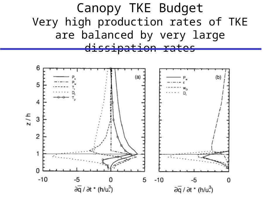
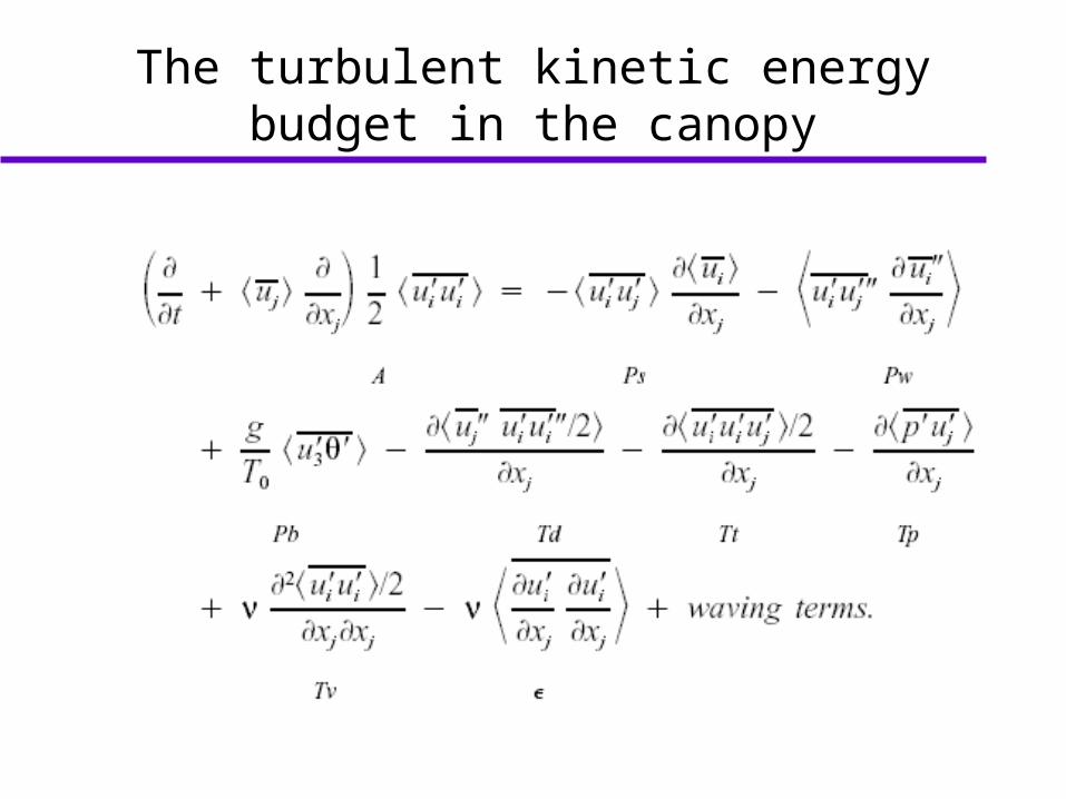
Canopy TKE BudgetVery high production rates of TKE are balanced

by very large dissipation rates

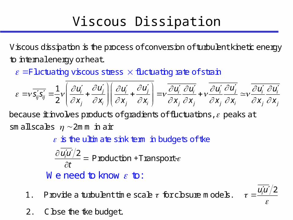
Viscous Dissipation

1

2

Viscous dissipation is the process of conversion of turbulent kinetic energy

to internal energy or he

Fluctuating viscous stress fluctuating rate of strain

at.

jiij ij

j i

uus s

x x

because it involves products of gradients of fluctuations

is the ultimate sink term

, peaks at

small scales

i

2mm in a

n

ir

b

j ji i i i i i

j i j j j i j j

u uu u u u u u

x x x x x x x x

2

2

Production +Transport-

1. Provide a turbulent time scale for closure models.

2. Close t

udgets

he tke budg

of tke

et.

We need to know to:

i

i

u u

t

u u

2 2

2

2

2

2

2

ji

j

i

i

k k j

i j

j

i k k

j k k j i

jj

j k k

i

j k

j

j

i

k j

uu u

x x x

u uu u u

x x x x x

u pu

x x x

u u

x x

u

u

x

ut

x

x

x

2

2

1

I I

ji k k

k k j i

i ij

k j k

j j

S S

uu u u

x x x x

u uu

x x x

v n dS dSV n

Vortex stretching by turbulent strain field

Vortex stretching by mean strain field

Pressure, turbulent and dispersive transport of <>

Destruction of <> by viscosity

Vortex stretching in the strain fields around plants and their wakes

Production/destruction of <> by coupling between local variations in mean viscous and Reynolds stresses

Canopy waving; flux of –ve vorticity from solid surfaces

The Canopy Dissipation Equation

+/-

++

+/-

+

- -

+/- -

++

How can we measure and parameterize the dissipation?

The problem: dissipation peaks at the Kolmogorov scale,

in the atmosphere so we can’t measure eddies of this scale with conventional instruments.

Instead we try to represent the dissipation in terms of the much larger and measurable eddies. To do this we need a model of the processes that transfer energy from the energy-containing to the dissipation scales.

This is why Kolmogorov’s theory is so important for experimentalists-it relates to the eddies in the ISR.

and mm1/ 43 2

Kolmogorov Spectrum for free-air turbulence

22

0

dS kk E k

dkdS k

dk

In the viscous subrange

In the inertial subrange (ISR),

Using dimensional and symmetry arguments, Kolmogorov (1941) found that in the ISR

2 3 2 3

2 3 5 3

Actually Kolmogorov worked with the structure function:

/ /

/ /

x, x r,u t u t r

E k k

Spectra measured in a spruce canopy by Amiro (1990)

Canopy spectra measured at high Re generally show 11(k1) rolling off more rapidly than –5/3 in the low frequency end of the ISR but not all data show this.

Isotropy in the ISR requires:

And this is usually violated in canopy data

22 33

11 11

1 1

1 1

4

3

k k

k k

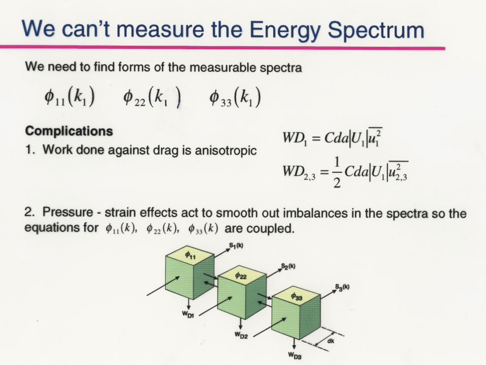
Do measurements show the predicted form?

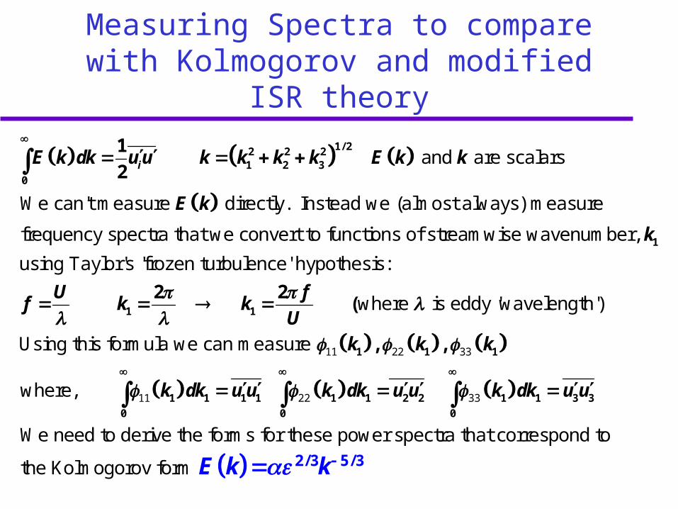
Measuring Spectra to compare with Kolmogorov and modified ISR theory

and are scalars

We can't measure directly. Instead we (almost always) measure

frequency spectra that we convert to functions of streamwise wavenumber,

using

1/ 22 2 21 2 3

0

1

1

2 iE k dk u u k k k k E k k

E k

k

11 22 33

11 22 33

Taylor's 'frozen turbulence' hypothesis:

where is eddy 'wavelength')

Using this formula we can measure

where,

1 1

1 1 1

1 1 1 1 1 1 2 2 1 1

0 0 0

2 2(

, ,

U ff k k

Uk k k

k dk u u k dk u u k dk

We need to derive the forms for these power spectra that correspond to

the Kolmogorov form

3 3

2/3 5/3

u u

E k k

Comparison of the theory with spectra from the Moga experiment, a 10m high uniform Eucalyptus forest.

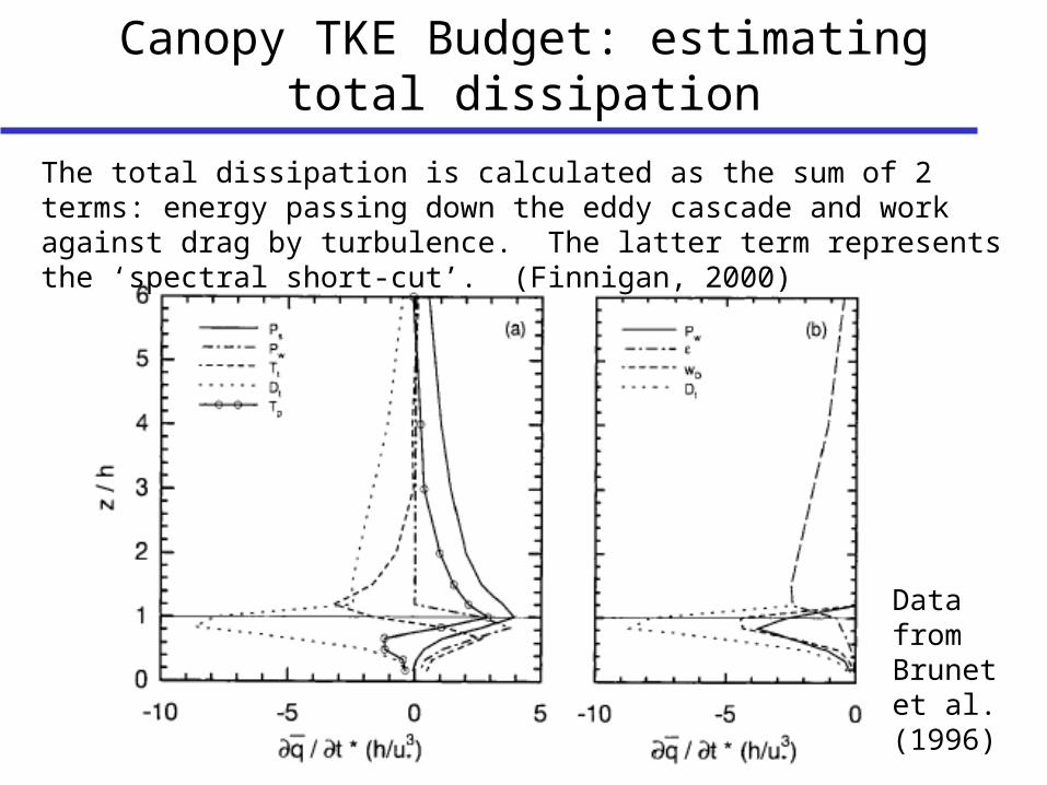
Canopy TKE Budget: estimating total dissipation

The total dissipation is calculated as the sum of 2 terms: energy passing down the eddy cascade and work against drag by turbulence. The latter term represents the ‘spectral short-cut’. (Finnigan, 2000)

Data from Brunet et al. (1996)

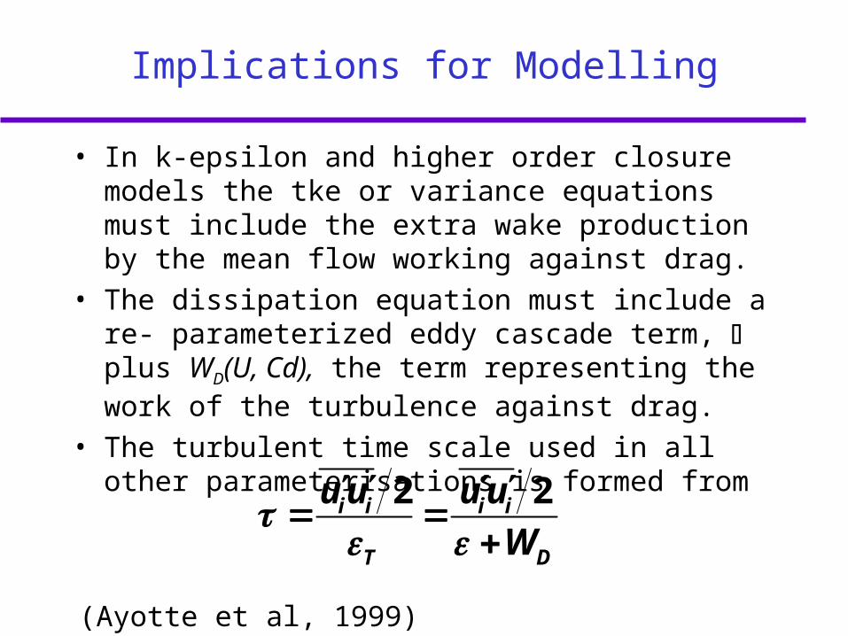
Implications for Modelling

• In k-epsilon and higher order closure models the tke or variance equations must include the extra wake production by the mean flow working against drag.

• The dissipation equation must include a re- parameterized eddy cascade term, plus WD(U, Cd), the term representing the work of the turbulence against drag.

• The turbulent time scale used in all other parameterisations is formed from

2 2i i i i

T D

u u u u

W

(Ayotte et al, 1999)

Conclusions

• tke in canopies finds it way to dissipation scales via the eddy cascade and via interaction with the canopy elements

• The assumptions of Kolmogorov theory for the form of E(k) in the ISR are violated because energy is continually lost as eddies do work against drag and the anisotropy of the drag ensures that the turbulence is at most axially symmetric, not isotropic

• We can treat the two routes to the dissipation scales separately but we must derive a new form for E(k) in the ISR that reflects these extra processes

• This form appears to predict the spectral levels and anisotropy of (two) canopy experiments quite well.

• The total dissipation is the sum of the energy passing down the eddy cascade (reduced compared to free air) and the work of the turbulence against drag

• This changes the turbulent time scale with implications for closure models.