Canonical Forms for Hamiltonian and SymplecticMatrices and Pencils

Wen-Wei Lin∗

Institute of Applied MathematicsNational Tsing Hwa University

Hsinchu, Taiwan, R. O. C.

Volker Mehrmann† and Hongguo Xu †

Fakultat fur MathematikTU Chemnitz

D-09107 Chemnitz, FR Germany.

Abstract

We study canonical forms for Hamiltonian and symplectic matrices or pencilsunder equivalence transformations which keep the class invariant. In contrast to othercanonical forms our forms are as close as possible to a triangular structure in the sameclass. We give necessary and sufficient conditions for the existence of Hamiltonianand symplectic triangular Jordan, Kronecker and Schur forms. The presented resultsgeneralize results of Lin and Ho [17] and simplify the proofs presented there.

Keywords. eigenvalue problem, Hamiltonian pencil (matrix), symplectic pencil (matrix),linear quadratic control, Jordan canonical form, Kronecker canonical form, algebraic Ric-cati equationAMS subject classification. 15A21, 65F15, 93B40

1 Introduction

In this paper we study canonical (Jordan and Kronecker) and condensed (Schur) formsfor matrices and matrix pencils with a special structure under equivalence transformationsthat keep this structure invariant. Let us first introduce the algebraic structures that weconsider.

∗This author was supported by NSC grant 87-2115-M007.†These authors were supported by Deutsche Forschungsgemeinschaft, Research Grant Me 790/7-2.

1

Let Jn :=

[0 In−In 0

], where In is the n × n identity matrix. We will just use J if the

size is clear from the context. The superscripts T , H represent the transpose and conjugatetranspose, respectively.

Definition 1

1. A matrix H ∈ C2n×2n is called Hamiltonian if HJn = (HJn)H . Every Hamiltonianmatrix can be expressed as

H =

[A DG −AH

], (1)

where D = DH and G = GH .

2. A matrix H ∈ C2n×2n is Hamiltonian triangular if H is Hamiltonian and in the blockform (1), with G = 0 and where A is upper triangular or quasi upper triangular if His real.

3. A matrix S ∈ C2n×2n is called symplectic if SHJnS = Jn.

4. A matrix S ∈ C2n×2n is symplectic triangular if it is symplectic and has the block

form S =

[S1 S2

0 S−H1

], where S1 is upper triangular or quasi upper triangular if S

is real.

5. A matrix pencilMh−λLh ∈ C2n×2n is called Hamiltonian ifMhJnLHh = −LhJnMHh .

6. A matrix pencil Mh − λLh ∈ C2n×2n is Hamiltonian triangular if it is Hamilto-

nian, Mh =

[M1 M3

0 M2

]and Lh =

[L1 L3

0 L2

], where M1,M

H2 , L1, L

H2 are upper

triangular. If the pencil is real then M1,MH2 are quasi upper triangular.

7. A matrix pencil Ms − λLs ∈ C2n×2n is called symplectic if MsJnMHs = LsJnLHs .

8. A matrix pencilMs−λLs ∈ C2n×2n is symplectic triangular if it is symplectic,Ms =[M1 M3

0 M2

]and Ls =

[L1 L3

0 L2

], where M1,M

H2 , L1, L

H2 are upper triangular. If

the pencil is real then M1,MH2 are quasi upper triangular.

9. A matrix Q ∈ C2n×2n is unitary symplectic if QHQ = I2n and QHJnQ = Jn.

Matrices and pencils with the structures introduced in Definition 1 occur in a large numberof applications. Classical applications are the solution of linear quadratic optimal controlproblems, where the matrices or matrix pencils associated with the two point boundaryvalue problems of Euler-Lagrangian equations have these structures [18], the solution ofH∞ control problems [8], eigenvalue problems in quantum mechanics [20] or the solution

2

of algebraic Riccati equations [2, 15]. While the Hamiltonian matrices form a Lie Algebra,the symplectic matrices form the corresponding Lie group.

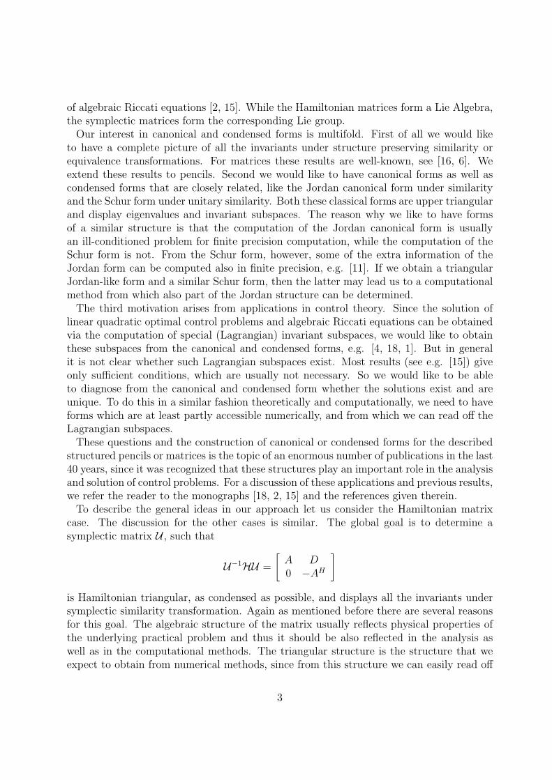
Our interest in canonical and condensed forms is multifold. First of all we would liketo have a complete picture of all the invariants under structure preserving similarity orequivalence transformations. For matrices these results are well-known, see [16, 6]. Weextend these results to pencils. Second we would like to have canonical forms as well ascondensed forms that are closely related, like the Jordan canonical form under similarityand the Schur form under unitary similarity. Both these classical forms are upper triangularand display eigenvalues and invariant subspaces. The reason why we like to have formsof a similar structure is that the computation of the Jordan canonical form is usuallyan ill-conditioned problem for finite precision computation, while the computation of theSchur form is not. From the Schur form, however, some of the extra information of theJordan form can be computed also in finite precision, e.g. [11]. If we obtain a triangularJordan-like form and a similar Schur form, then the latter may lead us to a computationalmethod from which also part of the Jordan structure can be determined.

The third motivation arises from applications in control theory. Since the solution oflinear quadratic optimal control problems and algebraic Riccati equations can be obtainedvia the computation of special (Lagrangian) invariant subspaces, we would like to obtainthese subspaces from the canonical and condensed forms, e.g. [4, 18, 1]. But in generalit is not clear whether such Lagrangian subspaces exist. Most results (see e.g. [15]) giveonly sufficient conditions, which are usually not necessary. So we would like to be ableto diagnose from the canonical and condensed form whether the solutions exist and areunique. To do this in a similar fashion theoretically and computationally, we need to haveforms which are at least partly accessible numerically, and from which we can read off theLagrangian subspaces.

These questions and the construction of canonical or condensed forms for the describedstructured pencils or matrices is the topic of an enormous number of publications in the last40 years, since it was recognized that these structures play an important role in the analysisand solution of control problems. For a discussion of these applications and previous results,we refer the reader to the monographs [18, 2, 15] and the references given therein.

To describe the general ideas in our approach let us consider the Hamiltonian matrixcase. The discussion for the other cases is similar. The global goal is to determine asymplectic matrix U , such that

U−1HU =

[A D0 −AH

]

is Hamiltonian triangular, as condensed as possible, and displays all the invariants undersymplectic similarity transformation. Again as mentioned before there are several reasonsfor this goal. The algebraic structure of the matrix usually reflects physical properties ofthe underlying practical problem and thus it should be also reflected in the analysis aswell as in the computational methods. The triangular structure is the structure that weexpect to obtain from numerical methods, since from this structure we can easily read off

3

eigenvalues and invariant subspaces. The maximal condensation, as in the standard Jordancanonical form, will give us the information about the invariants like the sizes of Jordanblocks and the eigen- and principal vectors.

There are many different approaches that one can take to derive canonical and condensedforms for Hamiltonian matrices. For the problems studied here, which are matrices fromclassical Lie and Jordan algebras a complete survey was given in [6], describing all thetypes of invariants that may occur. In this general framework, however, only the types ofinvariants are described, but not triangular forms or Schur forms.

Another very simple approach to obtain a canonical form is the idea to express theHamiltonian matrix H as a matrix pencil λJ −JH, i.e., a pencil where one of the matricesis skew Hermitian and the other is Hermitian. Using congruence transformations UH(λJ−JH)U , we obtain a canonical form via classical results for such pencils, see e.g., [22, 23].In view of our goals, however, this is not quite what we want, since in general these formsdo not give that UHJU = J , hence they do not lead to the structured form that we areinterested in. The other disadvantage of this approach is that it will not display directlythe Lagrangian subspaces, since it is not a triangular from.

Another classical approach is to use the pencil λiJ − JH, which is now a Hermitianpencil. Since iJ defines an indefinite scalar product, the elaborate theory of matricesin spaces with indefinite scalar products, e.g., [7] can be employed and the associatedcanonical forms can be obtained. This approach has been used successfully in the analysisof the algebraic Riccati equation [15] but shares the disadvantages with the approach viathe pencil λJ −JH. Another difficulty is that for real problems the problem is turned intoa complex problem due to the multiplication with i.

A canonical form under symplectic similarity directly for the Hamiltonian matrix wasfirst obtained in [16], but it has a very unusual structure which is not triangular or evennear triangular and it also cannot be used to determine the Lagrangian subspaces in asimple way.

A condensed form under unitary symplectic similarity transformations for Hamiltonianmatrices was first considered in [21]. These results were extended later in [17]. Otherstudies concerning canonical and condensed forms were given in [25, 26, 9].

The main motivation for our research arose from an unpublished technical report of Linand Ho on the existence of Hamiltonian Schur forms [17]. The results given there (for whichthe proofs are very hard to follow) are obtained as simple corollaries to our canonical form.

Particular emphasis in this paper is placed on the analysis of the eigenstructure associatedto eigenvalues on the imaginary axis in the Hamiltonian case, or on the unit circle in thesymplectic case, since this is where previous results did not give the complete analysis.Furthermore we derive our results from classical non-structured canonical forms.

The paper is structured as follows. In Section 2, we introduce the notation and givesome preliminary results. Section 3 gives some technical results which are needed for theconstruction of the canonical forms in the Hamiltonian case. Complex and real HamiltonianJordan forms are then presented in Section 4. The analogous results for Hamiltonian pencilsare presented in Section 5. In Section 6 we present again some technical results to dealwith the symplectic case. These results are then used to derive the canonical froms for

4

symplectic pencils in Section 7 and symplectic matrices in Section 8. The paper is writtenin such a way that the sections containing the canonical forms are essentially self containedand can be read without going through the technical lemmas in Sections 3 and 6.

2 Notation and preliminaries

In this section we introduce the notation and give some preliminary results.

Definition 2

1. A k−dimensional subspace U ⊆ Cn is called (right) invariant subspace for A ∈ Cn×n

if for a matrix U whose columns span U, there exists a matrix C ∈ Ck×k such thatAU = UC. It is called left invariant subspace for A ∈ Cn×n if it is an invariantsubspace for AH .

2. A k−dimensional subspace U ⊆ Cn is called (right) deflating subspace for a pencilA − λB ∈ Cn×n if for a matrix U whose columns span U, there exist matricesV ∈ Cn×k, C1, C2 ∈ Ck×k, such that AU = V C1, BU = V C2. It is called leftdeflating subspace for A−λB ∈ Cn×n if it is a right deflating subspace for AH−λBH .

3. A k−dimensional subspace U ⊆ C2n is called isotropic if xHJny = 0 for all x, y ∈ U.

4. A subspace U ⊆ C2n is called Lagrangian subspace if it is isotropic and is not con-tained in a larger isotropic subspace. A Lagrangian subspace always has dimensionn.

5. A subspace U ⊆ C2n is called Lagrangian invariant subspace of a matrix A ∈ Cn×n

if it is a (right) invariant subspace of A and is Lagrangian.

6. A subspace U ⊆ C2n×2n is called Lagrangian deflating subspace of the matrix pairA− λB if it is a (right) deflating subspace of A− λB and is Lagrangian.

The eigenvalues of Hamiltonian and symplectic matrices have certain symmetries. Al-though these properties are well-known, see e.g., [18], we list them following tables 1–4. Wewill use Λ(A) and Λ(A,B) to denote the spectrum and generalized spectrum of a squarematrix A and a matrix pencil A− λB, respectively. In the following tables the word evendenotes the fact that the algebraic multiplicity of an eigenvalue is even.

We will frequently use the following well-known properties of Hamiltonian and symplecticmatrices and pencils, see e.g., [18].

Proposition 1

1. If A is Hamiltonian (symplectic) and U is symplectic, then U−1AU is still Hamilto-nian (symplectic).

5

λ ∈ Λ(H) Complex Hamiltonian Real Hamiltonian

General Hamiltonian triangular General Hamiltonian triangular

Reλ 6= 0 −λ −λ λ,−λ,−λ λ,−λ,−λReλ = 0λ 6= 0

even −λ(= λ) λ,−λ even

λ = 0 even even even

Table 1: Eigenvalues of Hamiltonian matrices

λ ∈ Λ(Mh,Lh) Complex Hamiltonian Real Hamiltonian

General Hamiltonian triangular General Hamiltonian triangular

Reλ 6= 0 −λ −λ λ,−λ,−λ λ,−λ,−λReλ = 0λ 6= 0

even −λ(= λ) λ,−λ even

λ = 0 even even evenλ =∞ even even even

Table 2: Eigenvalues of Hamiltonian pencils

λ ∈ Λ(S) Complex symplectic Real symplectic

General Symplectic triangular General Symplectic triangular

|λ| 6= 1 λ−1 λ−1 λ, λ−1, λ−1 λ, λ−1, λ−1

|λ| = 1λ 6= ±1

even λ λ, λ even

λ = ±1 even even even

Table 3: Eigenvalues of symplectic matrices

λ ∈ Λ(Ms,Ls) Complex symplectic Real symplectic

General Symplectic triangular General Symplectic triangular

|λ| 6= 1, 0,∞ λ−1 λ−1 λ, λ−1, λ−1 λ, λ−1, λ−1

λ = 0, (∞) ∞, (0) 0,∞ even 0,∞ even|λ| = 1λ 6= ±1

even λ λ, λ even

λ = ±1 even even even

Table 4: Eigenvalues of symplectic pencils

6

2. If M− λL is Hamiltonian (symplectic), Y is nonsingular and U is symplectic, thenY(M− λL)U is Hamiltonian (symplectic).

Finally let us introduce two triangular factorizations that will be used frequently in thefollowing.

Lemma 3

1. For every matrix Z ∈ C2n×2n there exists a unitary matrix Q ∈ C2n×2n, such that

Z =

[R1,1 R1,2

0 R2,2

]Q, with R1,1, RH

2,2 upper triangular.

2. For every symplectic matrix S ∈ C2n×2n there exists a unitary symplectic matrix

Q ∈ C2n×2n, such that S = Q

[R1,1 R1,2

0 R−H1,1

], with R1,1 upper triangular.

For real matrices there are corresponding real factorizations.

Proof. The first part is a slight variation of the usual QL decomposition for ZH , see e.g.,[11] and the second part was proved in [3].

For completeness we also list the following well-known property of invariant subspaces,which follows directly from the Jordan canonical form, e.g. [10].

Proposition 2 Let A ∈ Cn×n, let the columns of U span the left invariant subspace ofA corresponding to λ1 ∈ Λ(A) and let the columns of V span the right invariant subspacecorresponding to λ2 ∈ Λ(A). If λ1 6= λ2 then UHV = 0. If λ1 = λ2 then det(UHV ) 6= 0.

Every Hermitian matrix A is congruent to its inertia matrix diag(Ip(A),−In(A), 0z(A)),where p(A), n(A), z(A) denote the number of positive, negative and zero eigenvalues of A.By Ind(A) we denote the tuple (1, . . . , 1︸ ︷︷ ︸

p(A)

,−1, . . . ,−1︸ ︷︷ ︸n(A)

, 0, . . . , 0︸ ︷︷ ︸z(A)

) associated with the inertia

matrix of A. We will also use the same notation for skew Hermitian matrices, i.e., fora skew Hermitian matrix A we denote by Ind(A) the tuple (i, . . . , i︸ ︷︷ ︸

p(A)

,−i, . . . ,−i︸ ︷︷ ︸n(A)

, 0, . . . , 0︸ ︷︷ ︸z(A)

),

where p(A), n(A), z(A) are the number of eigenvalues of A with positive, negative and zeroimaginary parts.

3 Technical lemmas for the Hamiltonian case

In this section we consider several technical results that are needed to derive the (Jordan)canonical form of a given Hamiltonian matrix H under symplectic similarity transforma-tions.

The goal is to determine a symplectic matrix U , such that

U−1HU =

[A D0 −AH

](2)

7

is Hamiltonian triangular, as condensed as possible, and displays all the invariants undersymplectic similarity transformation.

Lemma 4 Let H be symplectically similar to a Hamiltonian triangular matrix. Then thereexists a symplectic matrix U , such that

U−1HU =

[A D

0 −AH

], (3)

where A = diag(R1, . . . , Rµ, P1, . . . , Pν) and D = diag(0, . . . , 0, D1, . . . , Dν) are partitionedconformally. The blocks Pj are associated with the pairwise different purely imaginaryeigenvalues and the blocks Rj are associated with the pairwise different eigenvalues withnonzero real part, i.e., each block Pj has only one single purely imaginary eigenvalue iαjand αj 6= αk for j 6= k; analogously each block Rj has only one eigenvalue λj and λj 6= λkfor j 6= k.

Proof. By hypothesis there exists a symplectic matrix U1 such that

U−11 HU1 =

[A D0 −AH

].

Using the Jordan canonical form of A, there exists a nonsingular matrix T , such thatA := T−1AT = diag(R1, . . . , Rµ, P1, . . . , Pν) as desired. Then[

T−1 00 TH

]U−1

1 HU1

[T 00 T−H

]=

[A T−1DT−H

0 −AH

].

Using a sequence of symplectic similarity transformations with matrices of the form

[I Xj

0 I

],

where Xj is Hermitian, we can bring T−1DT−H to the desired block diagonal form D, seee.g., [18].

It follows that we can restrict the analysis of the Jordan and Schur forms for Hamilto-nian matrices to matrices with one single eigenvalue. In this way, we immediately obtainnecessary conditions for the invariant subspaces. The following result appeared first in anunpublished paper [17]. We will give a different proof.

Proposition 3 Let H be a Hamiltonian matrix, let iα1, . . . , iαν be its pairwise differentpurely imaginary eigenvalues and let Uk, k = 1, . . . , ν be matrices whose columns spanthe associated invariant subspaces. Analogously let λ1, . . . , λµ, −λ1, . . . ,−λµ be the pair-wise different eigenvalues with nonzero real parts and let Vk, Vk, k = 1, . . . , µ be matriceswhose columns span the associated invariant subspaces. If H is symplectically similar to aHamiltonian triangular matrix, then for all k = 1, . . . , µ, we have

V Hk JVk = 0, V H

k JVk = 0, det(V Hk JVk) 6= 0; (4)

and for all k = 1, . . . , ν, UHk JUk is congruent to Jlk for some integer lk.

8

Proof. By hypothesis we have (3). Partition the columns of U conformally with (3), i.e.,

U = [V1 . . . , Vµ, U1,1, . . . , U1,ν , V1, . . . , Vµ, U2,1, . . . , U2,ν ].

Obviously the columns of Uk := [U1,k, U2,k], k = 1, . . . , ν span the invariant subspacescorresponding to iαk, k = 1, . . . , ν and the columns of Vk, Vk span the invariant subspacescorresponding to Λ(Rk) and Λ(−RH

k ), respectively. The assertion then follows since U issymplectic.

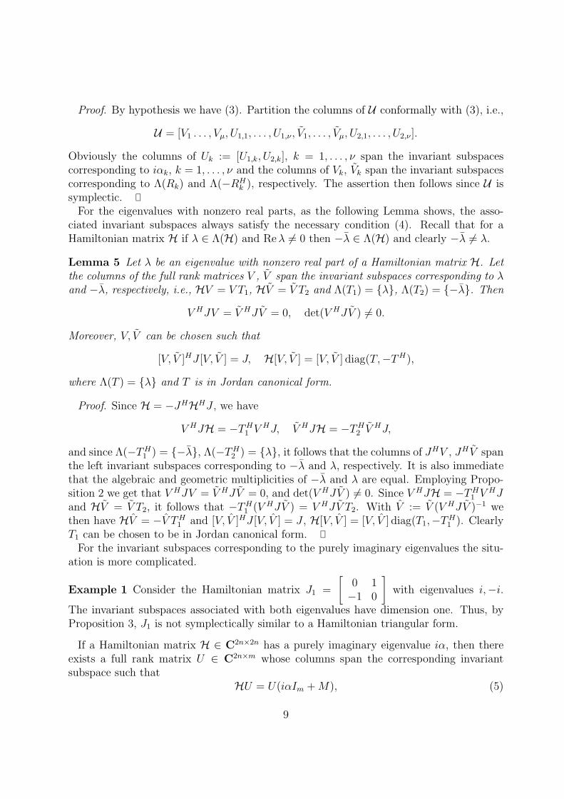
For the eigenvalues with nonzero real parts, as the following Lemma shows, the asso-ciated invariant subspaces always satisfy the necessary condition (4). Recall that for aHamiltonian matrix H if λ ∈ Λ(H) and Reλ 6= 0 then −λ ∈ Λ(H) and clearly −λ 6= λ.

Lemma 5 Let λ be an eigenvalue with nonzero real part of a Hamiltonian matrix H. Letthe columns of the full rank matrices V , V span the invariant subspaces corresponding to λand −λ, respectively, i.e., HV = V T1, HV = V T2 and Λ(T1) = λ, Λ(T2) = −λ. Then

V HJV = V HJV = 0, det(V HJV ) 6= 0.

Moreover, V, V can be chosen such that

[V, V ]HJ [V, V ] = J, H[V, V ] = [V, V ] diag(T,−TH),

where Λ(T ) = λ and T is in Jordan canonical form.

Proof. Since H = −JHHHJ , we have

V HJH = −TH1 V HJ, V HJH = −TH2 V HJ,

and since Λ(−TH1 ) = −λ, Λ(−TH2 ) = λ, it follows that the columns of JHV , JH V spanthe left invariant subspaces corresponding to −λ and λ, respectively. It is also immediatethat the algebraic and geometric multiplicities of −λ and λ are equal. Employing Propo-sition 2 we get that V HJV = V HJV = 0, and det(V HJV ) 6= 0. Since V HJH = −TH1 V HJand HV = V T2, it follows that −TH1 (V HJV ) = V HJV T2. With V := V (V HJV )−1 wethen have HV = −V TH1 and [V, V ]HJ [V, V ] = J , H[V, V ] = [V, V ] diag(T1,−TH1 ). ClearlyT1 can be chosen to be in Jordan canonical form.

For the invariant subspaces corresponding to the purely imaginary eigenvalues the situ-ation is more complicated.

Example 1 Consider the Hamiltonian matrix J1 =

[0 1−1 0

]with eigenvalues i,−i.

The invariant subspaces associated with both eigenvalues have dimension one. Thus, byProposition 3, J1 is not symplectically similar to a Hamiltonian triangular form.

If a Hamiltonian matrix H ∈ C2n×2n has a purely imaginary eigenvalue iα, then thereexists a full rank matrix U ∈ C2n×m whose columns span the corresponding invariantsubspace such that

HU = U(iαIm +M), (5)

9

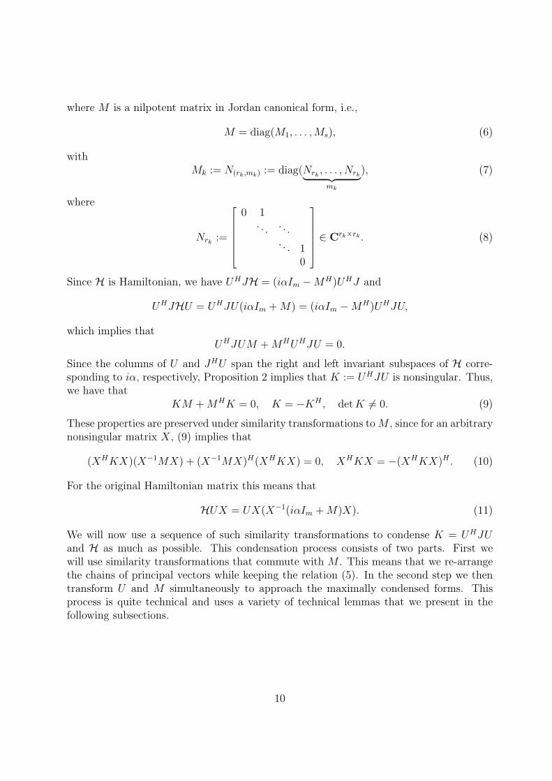
where M is a nilpotent matrix in Jordan canonical form, i.e.,

M = diag(M1, . . . ,Ms), (6)

withMk := N(rk,mk) := diag(Nrk , . . . , Nrk︸ ︷︷ ︸

mk

), (7)

where

Nrk :=

0 1

. . . . . .. . . 1

0

∈ Crk×rk . (8)

Since H is Hamiltonian, we have UHJH = (iαIm −MH)UHJ and

UHJHU = UHJU(iαIm +M) = (iαIm −MH)UHJU,

which implies thatUHJUM +MHUHJU = 0.

Since the columns of U and JHU span the right and left invariant subspaces of H corre-sponding to iα, respectively, Proposition 2 implies that K := UHJU is nonsingular. Thus,we have that

KM +MHK = 0, K = −KH , detK 6= 0. (9)

These properties are preserved under similarity transformations to M , since for an arbitrarynonsingular matrix X, (9) implies that

(XHKX)(X−1MX) + (X−1MX)H(XHKX) = 0, XHKX = −(XHKX)H . (10)

For the original Hamiltonian matrix this means that

HUX = UX(X−1(iαIm +M)X). (11)

We will now use a sequence of such similarity transformations to condense K = UHJUand H as much as possible. This condensation process consists of two parts. First wewill use similarity transformations that commute with M . This means that we re-arrangethe chains of principal vectors while keeping the relation (5). In the second step we thentransform U and M simultaneously to approach the maximally condensed forms. Thisprocess is quite technical and uses a variety of technical lemmas that we present in thefollowing subsections.

10

3.1 Matrices that commute with nilpotent Jordan matrices

In this section we recall some well-known results on matrices that commute with nilpotentmatrices in Jordan canonical form. We also present some technical lemmas.

Denote the set of all matrices that commute with a given nilpotent matrix N by G(N).This set is well studied, e.g., [12]. We recall a few results.

Proposition 4 Let Nr be as in (8) and let

Pr =

0 −1

(−1)2

·(−1)r 0

. (12)

Then

1. P−1r = PH

r = (−1)r−1Pr,

2. P−1r NH

r Pr = −Nr.

The similarity transformations that we consider are related to upper triangular Toeplitzmatrices of the form

T :=

τ0 τ1 . . . τr−1

. . . . . ....

. . . τ1

0 τ0

=r−1∑k=0

τkNkr . (13)

The diagonal element of such a matrix is denoted by θ(T ) := τ0. We have the followingwell-known Lemma, see Lemma 4.4.11 in [12].

Lemma 6 Let Nj, Nk be as in (8). A matrix E ∈ Cj×k satisfies NjE = ENk if and onlyif E has the form

E =

T j = k,[

0 T]j < k,[

T0

]j > k,

(14)

where T has the form (13).

For more complicated nilpotent matrices in Jordan form we have the following well-knownLemma, see [10, 12]. In the following we denote the set of j×k rectangular upper triangularToeplitz matrices E as in (14) by Gj×k.

Lemma 7 LetN = diag(Nr1 , . . . Nrs), (15)

where each Nrk is of the form (8). A matrix E commutes with N if and only if E has theblock structure E = [Ei,j]s×s, where each Ei,j ∈ Cri×rj is a rectangular upper triangularToeplitz matrix of the form (14).

11

For the nilpotent matrix N(r,m) as in (7), it follows that E ∈ G(N(r,m)) if and only if E hasthe block structure E = [Ei,j]m×m, partitioned conformally with N(r,m), where Ei,j ∈ Gr×r.Collecting the diagonal elements of each of the blocks in one matrix we obtain an m×mmatrix

Θ(E) :=

Θ(E1,1) . . . Θ(E1,m)

.... . .

...Θ(Em,1) . . . Θ(Em,m)

,which we call the main submatrix of E.

Lemma 8

1) If E1, E2 ∈ Gj×k, then E1 + E2 ∈ Gj×k.

2) If E1 ∈ Gj×k and E2 ∈ Gk×l, then E1E2 ∈ Gj×l. E1E2 is of full rank if and only ifE1, E2 both have full row rank (if j < l) or full column rank (if j ≥ l). Moreover,E1E2 is nonsingular if and only if E1 and E2 are square and nonsingular.

Proof. The first part is trivial. For the second part we only consider the case j ≥ l. Thecase j < l can be obtained in a similar way.

We have three subcases. If j < k then E1 =[

0 T1

], E2 =

[T2

0

], where T1 ∈ Cj×j,

T2 ∈ Cl×l are upper triangular Toeplitz matrices. If k ≥ j + l, then we have E1E2 = 0. If

k < j + l then E1E2 =

[T3

0

], where T3 =

[ k − j j + l − kj + l − k 0 T3

k − l 0 0

], and T3 is upper

triangular Toeplitz. Note that θ(T3) = θ(T1)θ(T2).

If j ≥ k ≥ l, then E1 =

[T1

0

], E2 =

[T2

0

], where T1 ∈ Ck×k, T2 ∈ Cl×l are upper

triangular Toeplitz. We then have E1E2 =

[T3

0

], where T3 ∈ Cl×l is upper triangular

Toeplitz and θ(T3) = θ(T1)θ(T2).

If k < l, then E1 =

[T1

0

], E2 =

[0 T2

], where T1 ∈ Ck×k, T2 ∈ Ck×k. We then obtain

E1E2 =

[T3

0

], where T3 =

[ l − k k

k 0 T3

l − k 0 0

], T3 ∈ Ck×k is upper triangular Toeplitz

and θ(T3) = θ(T1)θ(T2). Hence in all subcases E1E2 ∈ Gj×l and only in the second subcaseit is possible to have rank(E1E2) = l. So we need that j ≥ k ≥ l and θ(T1), θ(T2) 6= 0.Therefore, rank(E1) = k, rank(E2) = l. The reverse direction is obvious.

Lemma 9 Let E ∈ G(N) for N given in (15) and let P = diag(Pr1 , . . . , Prs).

1. If F ∈ G(N), then FE,EF ∈ G(N).

12

2. If E is nonsingular, then E−1 ∈ G(N).

3. P−1EHP ∈ G(N).

Proof. By definition of G(N) we have EN = NE.

1. Since FN = NF , we have EFN = ENF = NEF and thus, EF ∈ G(N). Similarlywe obtain FE ∈ G(N).

2. Since E is nonsingular, from EN = NE we have E−1N = NE−1 and thus E−1 ∈G(N).

3. By Proposition 4, P−1NHP = −N . Applying similarity transformations with P to(EN)H = (NE)H we obtain (P−1EHP )N = N(P−1EHP ) and hence P−1EHP ∈G(N).

Defining

Ω := [e1, er+1, . . . , e(m−1)r+1; e2, er+2, . . . , e(m−1)r+2; . . . ; er, e2r, . . . , emr],

where ek is the k-th unit vector, we have for each E ∈ G(N(r,m)), that

ω(E) := ΩTEΩ =

Θ(E) ∆1 . . . ∆r−1

. . . . . ....

. . . ∆1

0 Θ(E)

. (16)

This transformation sets up a one-to-one relationship between G(N(r,m)) and the set ofblock upper triangular Toeplitz matrices.

We then have the following result.

Lemma 10 Let M be as in (5) with the block sizes arranged in decreasing order, r1 >. . . > rs. Let

PM := diag(Pr1 , . . . , Pr1︸ ︷︷ ︸m1

, . . . , Prs , . . . , Prs︸ ︷︷ ︸ms

), (17)

with Pri defined as in (12). Let E ∈ G(M) and partition E conformally with the blockstructure of M in (6), i.e., E = [Ei,j]s×s and Ek,k ∈ G(N(rk,mk)). Let Θ(Ek,k) be the mainsubmatrices of the diagonal blocks Ek,k, k = 1, . . . , s. Then E is nonsingular if and only ifdet(Θ(Ek,k)) 6= 0, for all k = 1, . . . , s.

If E is nonsingular, then there exists a matrix Y ∈ G(M), such that

(P−1M Y HPM)EY =

E1,1 0

∗ E2,2...

. . . . . .

∗ . . . ∗ Es,s

, (18)

13

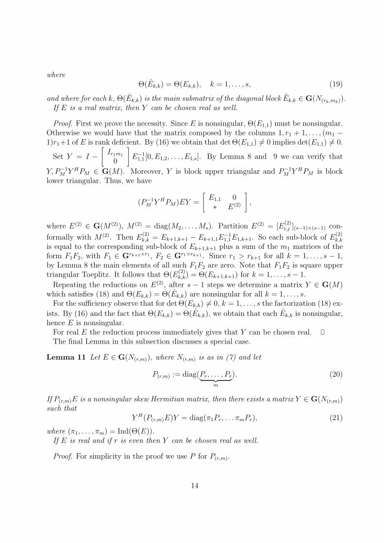
whereΘ(Ek,k) = Θ(Ek,k), k = 1, . . . , s, (19)

and where for each k, Θ(Ek,k) is the main submatrix of the diagonal block Ek,k ∈ G(N(rk,mk)).If E is a real matrix, then Y can be chosen real as well.

Proof. First we prove the necessity. Since E is nonsingular, Θ(E1,1) must be nonsingular.Otherwise we would have that the matrix composed by the columns 1, r1 + 1, . . . , (m1 −1)r1+1 of E is rank deficient. By (16) we obtain that det Θ(E1,1) 6= 0 implies det(E1,1) 6= 0.

Set Y = I −[Ir1m1

0

]E−1

1,1 [0, E1,2, . . . , E1,s]. By Lemma 8 and 9 we can verify that

Y, P−1M Y HPM ∈ G(M). Moreover, Y is block upper triangular and P−1

M Y HPM is blocklower triangular. Thus, we have

(P−1M Y HPM)EY =

[E1,1 0∗ E(2)

],

where E(2) ∈ G(M (2)), M (2) = diag(M2, . . . ,Ms). Partition E(2) = [E(2)i,j ](s−1)×(s−1) con-

formally with M (2). Then E(2)k,k = Ek+1,k+1 − Ek+1,1E

−11,1E1,k+1. So each sub-block of E

(2)k,k

is equal to the corresponding sub-block of Ek+1,k+1 plus a sum of the m1 matrices of theform F1F2, with F1 ∈ Grk+1×r1 , F2 ∈ Gr1×rk+1 . Since r1 > rk+1 for all k = 1, . . . , s − 1,by Lemma 8 the main elements of all such F1F2 are zero. Note that F1F2 is square uppertriangular Toeplitz. It follows that Θ(E

(2)k,k) = Θ(Ek+1,k+1) for k = 1, . . . , s− 1.

Repeating the reductions on E(2), after s − 1 steps we determine a matrix Y ∈ G(M)which satisfies (18) and Θ(Ek,k) = Θ(Ek,k) are nonsingular for all k = 1, . . . , s.

For the sufficiency observe that for det Θ(Ek,k) 6= 0, k = 1, . . . , s the factorization (18) ex-

ists. By (16) and the fact that Θ(Ek,k) = Θ(Ek,k), we obtain that each Ek,k is nonsingular,hence E is nonsingular.

For real E the reduction process immediately gives that Y can be chosen real.The final Lemma in this subsection discusses a special case.

Lemma 11 Let E ∈ G(N(r,m)), where N(r,m) is as in (7) and let

P(r,m) := diag(Pr, . . . , Pr︸ ︷︷ ︸m

). (20)

If P(r,m)E is a nonsingular skew Hermitian matrix, then there exists a matrix Y ∈ G(N(r,m))such that

Y H(P(r,m)E)Y = diag(π1Pr, . . . πmPr), (21)

where (π1, . . . , πm) = Ind(Θ(E)).If E is real and if r is even then Y can be chosen real as well.

Proof. For simplicity in the proof we use P for P(r,m).

14

Using the linear operator ω in (16), we obtain that E = ω(E) is block upper triangularToeplitz with diagonal block Θ(E). Moreover, we have

P = ω(P ) =

0 −Im

(−Im)2

·(−Im)r 0

.

Since PE is skew Hermitian, so is P E. Using the Kronecker product A⊗ B = [aijB], see

[14], E can be expressed as E =∑r−1k=0 N

kr ⊗ Ek, where E0 = Θ(E). By symmetry if r is

even, then E0, E2, . . . , Er−2 are Hermitian and E1, E3, . . . , Er−1 are skew Hermitian, andif r is odd, then E0, E2, . . . , Er−1 are skew Hermitian and E1, E3, . . . , Er−2 are Hermitian.Suppose that Y is a block upper triangular Toeplitz matrix with the same block structureas E. Let Y =

∑r−1k=0 N

kr ⊗ Yk. Using properties of the Kronecker product [14], we obtain

P−1Y HP =r−1∑k=0

(P−1r NH

r Pr)k ⊗ Y H

k =r−1∑k=0

(−1)kNkr ⊗ Y H

k ,

and hence

(P−1Y HP )EY =r−1∑k=0

Nkr ⊗

k∑p=0

(−1)pY Hp (

k−p∑q=0

Ek−p−qYq).

Here we have used that Nkr = 0 for k ≥ r. Now choose Y such that

(P−1Y HP )EY = Ir ⊗ Π, Π = diag(π1, . . . , πm). (22)

Then we have determined matrices Y0, . . . , Yr−1, such that for k = 1, . . . , r − 1,

Y H0 E0Y0 = Π, (23)

Y H0 E0Yk + (−1)kY H

k E0Y0 = −Ck, (24)

with

Ck =

Y0

Y1...

Yk−1

H

Ek Ek−1 . . . E1

−Ek−1 −Ek−2 . . . −E0...

... ·(−1)k−1E1 (−1)k−1E0 0

Y0

Y1...

Yk−1

.Since E0 = Θ(E), there exists a nonsingular matrix Y0 that satisfies (23). By the structureof Ek, in the case that r is even, we have that if k is even then Ck is Hermitian and if kis odd then Ck is skew Hermitian. In the case that r is odd, if k is even then Ck is skewHermitian and if k is odd then Ck is Hermitian. By (16), detE 6= 0 implies detE0 6= 0. Soin any case Yk can be chosen subsequently as Yk = −1

2(Y H

0 E0)−1Ck to satisfy (24). (Notethat the choice is not unique.)

Applying the inverse transform ω−1 on (22) and setting Y = ω−1(Y ), we obtain from(16) that Y ∈ G(N(r,m)) and

(P−1Y HP )EY = ω−1(Ir ⊗ Π) = diag(π1Ir, . . . , πmIr).

15

Pre-multiplying by P we have (21).If E is real and r is even, then since E0 = Θ(E) is real symmetric, Y0, Yk be chosen real

in (23) and (24). Therefore Y and also Y can be chosen real.Note that Θ(E) is Hermitian if r is even and it is skew Hermitian if r is odd. Thus

Ind(Θ(E)) consists of elements +1,−1, 0 if r is even and +i,−i, 0 if r is odd.

3.2 The structure of K

In this subsection we analyze the structure of skew Hermitian matrices K that satisfy (9)for a given nilpotent matrix M .

Lemma 12 Let M be a nilpotent matrix as in (6) and let K be as in (9). Then thereexists a matrix E ∈ G(M) such that K = PME with PM defined in (17).

Proof. By Proposition 4, P−1M MHPM = −M . Thus KM + MHK = 0 implies that

(P−1M K)M = M(P−1

M K). By definition of G(M) we then obtain P−1M K ∈ G(M).

Lemma 13 Let M be a nilpotent matrix as in (6) and let K be as in (9). Let E =[Ei,j]s×s ∈ G(M) be such that K = PME, where E is partitioned conformally with M =diag(M1, . . . ,Ms). If the index of Θ(Ek,k) is (πk,1, . . . , πk,mk) for k = 1, . . . , s, then thereexists a nonsingular matrix Y ∈ G(M) such that

Y HKY = diag(π1,1Pr1 , . . . , π1,m1Pr1 , . . . , πs,1Prs , . . . , πs,msPrs). (25)

If K is real and Y = [Y1, . . . , Ys] is partitioned in columns conformally with M , then Ykcan be chosen to be real for all k corresponding to an even rk.

Proof. Without loss of generality we may assume that r1 > . . . > rs.Lemma 12 implies that there exists a matrix E ∈ G(M), such that K = PME and, since

K is nonsingular, so is E. Hence we can employ Lemma 10. Since K = −KH , using (18),there exists Y1 ∈ G(M) so that

Y H1 KY1 = PM(P−1

M Y H1 PM)EY1 = PM diag(E1,1, . . . , Es,s)

= diag(P(r1,m1)E1,1, . . . , P(rs,ms)Es,s),

where P(rk,mk) is defined as in (20). Moveover, for all k = 1, . . . , s the matrix P(rk,mk)Ek,kis skew Hermitian. Applying Lemma 11, for each P(rk,mk)Ek,k there exists a matrix Yk ∈G(N(rk,mk)), such that

Y Hk (P(rk,mk)Ek,k)Yk = diag(πk,1Prk , . . . , πk,mkPrk),

where(πk,1, . . . , πk,mk) = Ind(Θ(Ek,k)) = Ind(Θ(Ek,k)).

The last equality follows from Lemma 10.Set Y2 := diag(Y1, . . . , Ys) then Y2 ∈ G(M) and also Y := Y1Y2 ∈ G(M). Furthermore

Y HKY has the form (25).The real case follows from the corresponding real parts in Lemmas 10 and 11.

16

Remark 1 The matrices Y ∈ G(M) constructed in the proof of Lemma 10 and 11 are ingeneral not unique.

Notice that (πk,1, . . . , πk,mk) is the inertia index of Θ(Ek,k). But by Lemma 10, for allk = 1, . . . , s, Θ(Ek,k) is invariant under congruence transformations with Y ∈ G(M). Soall these indices are uniquely determined by the matrices K and M . Hence (25) can beviewed as the canonical form of K under congruence transformations in G(M).

From the beginning of the construction we see that the matrices K, M contain the char-acteristic quantities associated with the eigenvalues of iα of H, in particular the numberand sizes of Jordan blocks. Based on these quantities we set

βk,j :=

(−1)rk2 πk,j, if rk is even,

(−1)rk−1

2 iπk,j, otherwise.(26)

Note that by construction βk,j ∈ 1,−1.

Definition 14 Let πk,j be as in (25) and βk,j as in (26), then the tuple

IndS(iα) := (β1,1, . . . , β1,m1 , . . . , βs,1, . . . , βs,ms) (27)

is called the structure inertia index of the eigenvalue iα.

It is not surprising that certain signs associated with Jordan blocks to purely imaginaryeigenvalues will be important. These signs obviously occur in the approaches to obtaincanonical forms for Hermitian pencils as studied in [7, 22] or in the analysis of Lagrangiansubspaces [9]. These signs are sometimes called sign characteristics and they play the keyrole in determining the structure of the Hamiltonian Jordan canonical form and in thesolvability theory for algebraic Riccati equations [15].

By Lemma 13 we have obtained a partition of a matrix K as in (9) into m =∑sk=1 mk

submatrices of the form πk,jPrk , where πk,j ∈ 1,−1 if r is even and πk,j ∈ i,−i if r isodd. Each πk,jPrk corresponds to a nilpotent block Nrk in the Jordan canonical form. Inother words, by the above construction we have obtained all chains of principal vectors Uof H corresponding to all the single Jordan blocks satisfying UHJU = πk,jPrk .

3.3 Combining Jordan blocks to Hamiltonian Jordan blocks

Since the matrix pair (K,M) from (9) can be decoupled in blocks (πk,jPrk , Nrk) associatedwith Jordan blocks which are in general not Hamiltonian, we will now describe possibilitiesto combine or split such Jordan blocks to Hamiltonian Jordan blocks.

Lemma 15

1. For a pair (πP2r, N2r), with π = (−1)rβ and β ∈ 1,−1, let Ze := diag(Ir, πP−1r ).

Then

ρe(πP2r, N2r) := (ZHe (πP2r)Ze, Z

−1e N2rZe)

=

([0 Ir−Ir 0

],

[Nr βere

Hr

0 −NHr

]). (28)

17

2. For a pair (πP2r+1, N2r+1), with π = (−1)r+1iβ and β ∈ 1,−1, let

Zo(r) := diag(Ir+1, (πPr)−1). (29)

Then

ρo(πP2r+1, N2r+1) := (Zo(r)H(πP2r+1)Zo(r), Zo(r)

−1N2r+1Zo(r))

=

0 0 Ir

0 iβ 0−Ir 0 0

, Nr er 0

0 0 iβeHr0 0 −NH

r

. (30)

Proof. We can rewrite the matrix pair (πP2r, N2r) as([0 πPr

(−1)rπPr

],

[Nr ere

H1

0 Nr

]).

Then we obtain (28) by Proposition 4.Similarly we can rewrite (πP2r+1, N2r+1) as

0 0 πPr0 iβ 0

(−1)r+1πPr 0 0

, Nr er 0

0 0 eH10 0 Nr

and with the given Zo(r) we obtain (30).For an even size matrix pair (πPr, Nr) the transformation ρe yields a pair of the form

(Jr, Tr) with a Hamiltonian triangular matrix Tr. For a single odd size matrix pair, however,we cannot obtain such a form, since J has even size. Thus, it is a natural idea to combinetwo odd size pairs associated with (possibly different) purely imaginary eigenvalues iα1, iα2.

In the following we will use the notation Nk(λ) := λI +Nk.

Lemma 16 Given two matrix pairs (πkP2rk+1, N2rk+1(iαk)) for k = 1, 2, with αk real,πk = (−1)rk+1iβk and βk ∈ 1,−1. Let

(Pc, Nc) :=

([π1P2r1+1 0

0 π2P2r2+1

],

[N2r1+1(iα1) 0

0 N2r2+1(iα2)

]),

V :=

[v1,1 v1,2

v2,1 v2,2

]:=√

22

[−1 iβ1

−1 −iβ1

]and

Zc :=

[Zo(r1) 0

0 Zo(r2)

]

Ir1 0 0 0 0 00 0 v1,1 0 0 v1,2

0 0 0 Ir1 0 00 Ir2 0 0 0 00 0 v2,1 0 0 v2,2

0 0 0 0 Ir2 0

. (31)

18

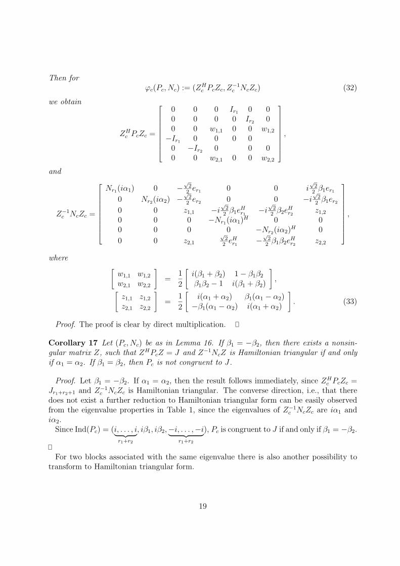
Then forϕc(Pc, Nc) := (ZH

c PcZc, Z−1c NcZc) (32)

we obtain

ZHc PcZc =

0 0 0 Ir1 0 00 0 0 0 Ir2 00 0 w1,1 0 0 w1,2

−Ir1 0 0 0 00 −Ir2 0 0 00 0 w2,1 0 0 w2,2

,

and

Z−1c NcZc =

Nr1(iα1) 0 −√

22er1 0 0 i

√2

2β1er1

0 Nr2(iα2) −√

22er2 0 0 −i

√2

2β1er2

0 0 z1,1 −i√

22β1e

Hr1

−i√

22β2e

Hr2

z1,2

0 0 0 −Nr1(iα1)H 0 00 0 0 0 −Nr2(iα2)H 0

0 0 z2,1

√2

2eHr1 −

√2

2β1β2e

Hr2

z2,2

,

where [w1,1 w1,2

w2,1 w2,2

]=

1

2

[i(β1 + β2) 1− β1β2

β1β2 − 1 i(β1 + β2)

],[

z1,1 z1,2

z2,1 z2,2

]=

1

2

[i(α1 + α2) β1(α1 − α2)−β1(α1 − α2) i(α1 + α2)

]. (33)

Proof. The proof is clear by direct multiplication.

Corollary 17 Let (Pc, Nc) be as in Lemma 16. If β1 = −β2, then there exists a nonsin-gular matrix Z, such that ZHPcZ = J and Z−1NcZ is Hamiltonian triangular if and onlyif α1 = α2. If β1 = β2, then Pc is not congruent to J .

Proof. Let β1 = −β2. If α1 = α2, then the result follows immediately, since ZHc PcZc =

Jr1+r2+1 and Z−1c NcZc is Hamiltonian triangular. The converse direction, i.e., that there

does not exist a further reduction to Hamiltonian triangular form can be easily observedfrom the eigenvalue properties in Table 1, since the eigenvalues of Z−1

c NcZc are iα1 andiα2.

Since Ind(Pc) = (i, . . . , i︸ ︷︷ ︸r1+r2

, iβ1, iβ2,−i, . . . ,−i︸ ︷︷ ︸r1+r2

), Pc is congruent to J if and only if β1 = −β2.

For two blocks associated with the same eigenvalue there is also another possibility totransform to Hamiltonian triangular form.

19

Lemma 18 Given two matrix pairs (πkPrk , Nrk), k = 1, 2, where r1, r2 are either botheven or both odd. Let for k = 1, 2, πk ∈ 1,−1 if both rk are even and πk ∈ i,−i if bothrk are odd. Let

(Pc, Nc) :=

([π1Pr1 0

0 π2Pr2

],

[Nr1 00 Nr2

])

and d := |r1−r2|2

. If π1 = (−1)d+1π2, i.e., β1 = −β2 for the corresponding β1 and β2, thenwe have the following transformations.

1. If r1 ≥ r2 then with

Z1 :=

Id 0 0 0

0√

22Ir2 0 −

√2

2π2P

−1r2

0 0 π1P−1d 0

0 −√

22Ir2 0 −

√2

2π2P

−1r2

we obtain for ϕ1(Pc, Nc) := (ZH

1 PcZ1, Z−11 NcZ1) that ZH

1 PcZ1 = J r1+r22

and

Z−11 NcZ1 =

Nd

√2

2ede

H1 0 −

√2

2π2ede

Hr2

0 Nr2 −√

22π2er2e

Hd 0

0 0 −NHd 0

0 0 −√

22e1e

Hd −NH

r2

. (34)

2. If r1 < r2, then with

Z2 =

√

22π1Pr1 0

√2

2Ir1 0

0 π2Pd 0 0

−√

22π1Pr1 0

√2

2Ir1 0

0 0 0 Id

we obtain for ϕ2(Pc, Nc) := (ZH

2 PcZ2, Z−12 NcZ2) that ZH

2 PcZ2 = J r1+r22

and

Z−12 NcZ2 =

−NH

r10 0 −

√2

2π1e1e

H1

−√

22e1e

Hr1−NH

d −√

22π1e1e

H1 0

0 0 Nr1

√2

2er1e

H1

0 0 0 Nd

. (35)

Proof. The proof follows directly by multiplying out the products.

Remark 2 It is very difficult to compare the different possibilities to combine blocks toHamiltonian form. First of all the form (35) is not of the triangularity structure thatwe want, while the from (34) is of the right triangularity structure and actually is morecondensed than the form obtained in Lemma 16.

20

The invariant subspaces are also different, when using transformations ρe, ρo, ϕ1, ϕ2 orϕc. This is demonstrated in the following simple example.

Let H be a nilpotent Hamiltonian matrix with two Jordan blocks N2r1 and N2r2 , andr1 ≥ r2. Then there exist corresponding matrices V1 = [V1,1, V1,2, V1,3, V1,4], V2 = [V2,1, V2,2],where V1,2, V1,3, V2,1, V2,2 ∈ C2(r1+r2)×r2 and V1,1, V1,4 ∈ C2(r1+r2)×(r1−r2), so that for k = 1, 2,

HVk = VkN2rk , V Hk JVk = πkP2rk .

Suppose that the structure inertia index associated with the eigenvalue 0 is IndS(0) =

(1,−1). Then we can determine different symplectic matrices U such thatHU = U[R D0 −RH

].

First we use ρe of Lemma 15. Then U := [U1, U2] with U1 =[

[V1,1, V1,2] V2,1

]and

U2 =[

[V1,3, V1,4](π1Pr1)−1, V2,2(π2Pr2)−1].

Note that U1, which spans a Lagrangian invariant subspace of H, is composed from thefirst halves of the chains of principal vectors corresponding to N2r1 and N2r2 respectively.

Using ϕ1 we get U1 =[V1,1

√2

2[V1,2 − V2,1, V1,3 − V2,2]

], which is composed from the

first r1 + r2 principal vectors corresponding to N2r1 and all principal vectors correspondingto N2r2 . Using ϕ2 we get the same subspaces.

Clearly the two related Lagrangian invariant subspaces are different even for r1 = r2. Asimilar example can be easily constructed if H has two odd size Jordan blocks.

We will now use the construction described in Lemma 15 to Corollary 17 to characterizea condensed form that is near to a Hamiltonian triangular form, i.e., a matrix U so thatHU = UT in (5), with Λ(T ) = iα and T is near to a Hamiltonian triangular form.

Lemma 19 Let iα be an eigenvalue of the Hamiltonian matrix H. Then there exists amatrix U = [U1, U2, U3] of full column rank, such that HU = UT , where U , T satisfy

UHJU =

0 0 I 0 00 0 0 I 0−I 0 0 0 00 −I 0 0 0

0 0 0 0 K

, T =

R1 0 D1 0 00 R2 0 D2 00 0 −RH

1 0 00 0 0 −RH

2 00 0 0 0 R3

, (36)

with K = diag(πd1P2t1+1, . . . , πdzP2tz+1) and R3 = diag(N2t1+1(iα), . . . , N2tz+1(iα)). The

matrices R1, R2, D1, D2 are substructured further as

R1 = diag(Nl1(iα), . . . , Nlq(iα)), D1 = diag(βe1el1eHl1, . . . , βeqelqe

Hlq ),

R2 = diag(B1, . . . , Br), D2 = diag(C1, . . . , Cr),

where for k = 1, . . . , r

Bk =

Nmk(iα) 0 −√

22emk

Nnk(iα) −√

22enk

iα

,21

Ck =

√2

2iβck

0 0 emk0 0 −enk−eHmk eHnk 0

.Furthermore the structure inertia index also consists of three parts,

IndS(iα) = (IndeS(iα), IndcS(iα), InddS(iα)),

where

1. IndeS(iα) := (βe1, . . . , βeq) corresponds to even size Jordan blocks N2lk(iα), k = 1, . . . , q

which are contained in

[R1 D1

0 −RH1

];

2. IndcS(iα) := (βc1, . . . , βcr ;−βc1, . . . ,−βcr) corresponds to odd size Jordan blocks N2m1+1(iα),

. . . , N2mr+1(iα), N2n1+1(iα), . . . , N2nr+1(iα), which are coupled as pairs([πkP2mk+1 0

0 ((−1)|mk−nk|+1πk)P2nk+1)

],

[N2mk+1(iα) 0

0 N2nk+1(iα)

])

and contained in

[R2 D2

0 −RH2

];

3. InddS(iα) := (βd1 , . . . , βdz ) = ((−1)t1iπd1 , . . . , (−1)tz iπdz) with βd1 = . . . = βdz . This part

corresponds to the Jordan blocks in R3.

Proof. Let the columns of X span the invariant subspace of H corresponding to iαand suppose that X satisfies (5) - (8). Applying Lemma 13 to K := XHJX we get atransformation matrix Y , such that Y HKY has the form (25). We then perform furthertransformations as in Lemma 15–Corollary 17 to the pairs of the form (πPr, Nr) as theyarise in (25).

For even r we use ρe defined in (28), which implies that there exists a matrix Xr, suchthat

XHr JXr = J, HXr = Xr(Z

−1e Nr(iα)Ze).

For odd r we combine together as many pairs as possible of the form (π1P2r1+1, N2r1+1(iα))together with (π2P2r2+1, N2r2+1(iα)), so that the corresponding β1 and β2 satisfy β1 = −β2.Using ϕc in (32), there exists a matrix Xr1,r2 such that (note that the eigenvalues are same)

XHr1,r2

JXr1,r2 = J, HXr1,r2 = Xr1,r2(Z−1c diag(N2r1+1(iα), N2r2+1(iα))Zc).

Grouping the first half of the columns of all the Xr and Xr1,r2 together in U1 and thesecond half of the columns in U2, using the same order and forming U3 by grouping all thechains of principal vectors corresponding to the remaining odd size matrices (all havingthe same sign β) we can form U := [U1, U2, U3] and we can easily verify (36).

22

Remark 3 Note that the factorization (36) is in general not unique. If several structureinertia indices for odd size Jordan blocks have opposite signs or if as in Lemma 18 twomatrix pairs with opposite signs of the indices are grouped then we may get a differentfactorization.

The non-uniqueness implies that IndcS(iα) and InddS(iα) can be selected in many ways inthe sense that the elements can correspond to different Jordan blocks with different sizes.However, by our construction all odd size pairs of indices with opposite sign are groupedin IndcS(iα) and all remaining indices in InddS(iα). For a given iα, IndcS(iα) always containsthe same number of 1 and −1 and InddS(iα) contains elements with all 1 or −1. So thenumber of elements and the signs of IndcS(iα) and InddS(iα) are uniquely determined.

4 Hamiltonian Jordan canonical forms

Using the technical results from the previous section, we are now ready to derive thecanonical forms for Hamiltonian matrices under symplectic similarity transformations.

Theorem 20 (Hamiltonian Jordan canonical form) Given a complex Hamiltonian ma-trix H, there exists a complex symplectic matrix U such that

U−1HU =

Rr 0Re De

Rc Dc

Rd Dd

0 −RHr

0 −RHe

0 −RHc

Gd −RHd

, (37)

where the different blocks have the following structures.1. The blocks with index r are associated with the pairwise distinct eigenvalues with

nonzero real part λ1, . . . , λµ,−λ1, . . . ,−λµ of H. The Jordan blocks associated with λk(−λk) have the form

Rr = diag(Rr1, . . . , R

rµ), Rr

k = diag(Ndk,1(λk), . . . , Ndk,pk(λk)), k = 1, . . . , µ.

2. The blocks with indices e and c are associated with pairwise distinct purely imag-inary eigenvalues iα1, . . . , iαν grouped together in such a way that the structure inertiaindices satisfy IndeS(iαk) = (βek,1, . . . , β

ek,qk

), which are associated with even sized blocks andIndcS(iαk) = (βck,1, . . . , β

ck,rk

,−βck,1, . . . ,−βck,rk) which are associated with paired odd sizedblocks. These blocks have the following substructures.

Re = diag(Re1, . . . , R

eν), Re

k = diag(Nlk,1(iαk), . . . , Nlk,qk(iαk)),

De = diag(De1, . . . , D

eν), De

k = diag(βek,1elk,1eHlk,1, . . . , βek,qkelk,qke

Hlk,qk

),

Rc = diag(Rc1, . . . , R

cν), Rc

k = diag(Bk,1, . . . , Bk,rk),

Dc = diag(Dc1, . . . , D

cν), Dc

k = diag(Ck,1, . . . , Ck,rk),

23

where for k = 1, . . . , ν and j = 1, . . . , rk we have

Bk,j =

Nmk,j(iαk) 0 −√

22emk,j

0 Nnk,j(iαk) −√

22enk,j

0 0 iαk

,

Ck,j =

√2

2iβck,j

0 0 emk,j0 0 −enk,j

−eHmk,j eHnk,j 0

.3. The blocks with index d are associated with two disjoint sets of purely imaginary eigen-

values iγ1, . . . , iγη, iδ1, . . . , iδη ⊆ iα1, . . . , iαν, such that the corresponding structureinertia indices are (βd1 , . . . , β

dη), (−βd1 , . . . ,−βdη) with βd1 = . . . = βdη . The blocks have the

following substructures.

Rd = diag(Rd1, . . . , R

dη), Dd = diag(Dd

1, . . . , Ddη), Gd = diag(Gd

1, . . . , Gdη),

where for k = 1, . . . , η

Rdk =

Nsk(iγk) 0 −√

22esk

0 Ntk(iδk) −√

22etk

0 0 i2(γk + δk)

,

Ddk =

√2

2iβdk

0 0 esk0 0 −etk−eHsk eHtk −i

√2

2(γk − δk)

,

Gdk = βdk

0 0 00 0 00 0 −1

2(γk − δk)

.Proof. Using Lemma 5, for each eigenvalue λk with nonzero real part, we can determine

a matrix Qk = [Qk,1, Qk,2], such that

QHk JQk = J, HQk = Qk diag(Rr

k,−(Rrk)H),

where Rrk is the Jordan canonical form associated with the eigenvalue λk.

Using Lemma 19, for each purely imaginary eigenvalue iαk, we can determine a matrixUk = [Uk,1, Uk,2, Uk,3], such that

UHk JUk =

0 I 0−I 0 0

0 0 Kk

, HUk = Uk

Rek 0 De

k 0 00 Rc

k 0 Dck 0

0 0 −(Rek)H 0 0

0 0 0 −(Rck)H 0

0 0 0 0 Rk,3

,

has the structure as in (36). Moreover, in the structure inertia index InddS(iαk) (corre-sponding to Kk) all elements βk,1, . . . , βk,ζk have the same sign.

24

Let X = [Q1, . . . , Qµ, U1, . . . , Uν ]. Since the columns of each of the blocks span invariantsubspaces of distinct eigenvalues, X is nonsingular, and hence Ind(XHJX) has the samenumber of elements i and −i.

By Lemmas 5, 15 and 16, each of the inertias Ind(QHk JQk), Ind([Uk,1, Uk,2]HJ [Uk,1, Uk,2])

contains the same numbers of elements i and −i. Also for each Uk,3, Ind(UHk,3JUk,3) contains

the same numbers of elements i and −i and the additional elements are iβk,1,. . . , iβk,ζk .Note that

XHJX = diag(Jnr1 , . . . , Jnrµ ; Jne1 , Jnc1 , K1, . . . , Jneν , Jncν , Kν),

where nrk =∑pkj=1 dk,j, n

ek =

∑qkj=k lk,j and nck =

∑rkj=1(mk,j + nk,j + 1), for k = 1, . . . , ν.

Taking all the iβk,j, j = 1, . . . , ζk, k = 1, . . . , ν together, there must be an equal number

of elements i and −i. This implies that we can group all the pairs (Kk, Rk,3) in couples oftwo with opposite structure inertia indices. Applying ϕc as in Lemma 16 to these coupleswe can determine matrices Wk = [Wk,1,Wk,2], such that

WHk JWk = J, HWk = Wk

[Rdk Dd

k

Gdk −(Rd

k)H

].

Partition Uk,1 = [Vk,1, Vk,2], Uk,2 = [Vk,1, Vk,2] in columns according to the block sizes ofRek and Rc

k, respectively and set

U = [Q1,Ve1 ,Vc1,W1,Q2,Ve2 ,Vc2,W2],

where

Q1 = [Q1,1, . . . , Qµ,1], Ve1 = [V1,1, . . . , Vν,1],

Vc1 = [V1,1, . . . , Vν,1], W1 = [W1,1, . . . ,Wη,1],

Q2 = [Q1,2, . . . , Qµ,2], Ve2 = [V1,2, . . . , Vν,2],

Vc = [V1,2, . . . , Vν,2], W2 = [W1,2, . . . ,Wη,2].

Then by Proposition 2, U is symplectic and U−1HU has the form (37).For a real Hamiltonian matrix H, we would like to have a real canonical form. As for the

classical Jordan canonical form, we combine eigenvectors and principals vectors associatedwith complex conjugate pairs. Introducing the matrices

Ψ2r = [e1, er+1, e2, er+2, . . . , er, e2r], Φ2r = diag(Φ2,Φ2, . . . ,Φ2︸ ︷︷ ︸r

), (38)

where

Φ2 =

√2

2

[1 −i1 i

],

we have the following trivial lemma.

Lemma 21

25

1. Let A = [ai,j] be a complex r × r matrix. Then

(Ψ2rΦ2r)H

[A 00 A

](Ψ2rΦ2r) := [Bi,j],

is a real block matrix with 2× 2 blocks

Bi,j =

[Re aij, Im ai,j− Im ai,j Re ai,j

], i, j = 1, . . . , r.

2. If U is a complex n× r matrix, then [U, U ]Ψ2rΦ2r is real.

To simplify the notation in the real Jordan canonical form, we set in the following

Nr(Λ) =

Λ I 0

. . . . . .. . . I

0 Λ

, (39)

where either Λ is a real scalar and the identity matrices have size 1× 1 or Λ =

[a b−b a

]with a, b real and the identity matrices have size 2 × 2. For the latter case we haveNr(Λ) ∈ C2r×2r.

Theorem 22 (Real Hamiltonian Jordan canonical form) Given a real Hamiltonianmatrix H, there exists a real symplectic matrix U such that

U−1HU =

Rr 0Re De

Rc Dc

R0 D0

Rd Dd

0 −RTr

0 −RTe

0 −RTc

0 −RT0

Gd −RTd

, (40)

where the different blocks have the following structures.1. The blocks with index r are associated with the pairwise distinct eigenvalues with

nonzero real part. The diagonal blocks have the form Λk, where either Λk is a nonzero real

number, or Λk =

[ak bk−bk ak

], ak, bk real and nonzero. In the first case Λk and −Λk are

both nonzero real eigenvalues of H, with sizes of Jordan blocks dk,1, . . . , dk,pk . In the second

26

case λk = ak + ibk, together with λk, −λk,−λk, are the eigenvalues of H and each has thesame sizes of Jordan blocks dk,1, . . . , dk,pk . We have

Rr = diag(Rr1, . . . , R

rµ),

Rrk = diag(Ndk,1(Λk), . . . , Ndk,pk

(Λk)), k = 1, . . . , µ.

2. The blocks with indices e, c, d are associated with the pairwise distinct, nonzero, purelyimaginary eigenvalues iαk, −iαk, k = 1, . . . , ν. For each k = 1, . . . , ν the associatedstructure inertia indices are

IndeS(iαk) = (βek,1, . . . , βek,qk

),

IndcS(iαk) = (βck,1, . . . , βck,rk

,−βck,1, . . . ,−βck,rk),InddS(iαk) = (βdk , . . . , β

dk︸ ︷︷ ︸

sk

),

IndeS(−iαk) = (βek,1, . . . , βek,qk

),

IndcS(−iαk) = (−βck,1, . . . ,−βck,rk , βck,1, . . . , β

ck,rk

),

InddS(−iαk) = (−βdk , . . . ,−βdk︸ ︷︷ ︸sk

),

and (with the notation Σk =

[0 αk−αk 0

], αk 6= 0,) for k = 1, . . . , ν the substructures are

Re = diag(Re1, . . . , R

eν), De = diag(De

1, . . . , Deν),

Rek = diag(Nlk,1(Σk), . . . , Nlk,qk

(Σk)),

Dek = diag(βek,1

[0 00 I2

]2lk,1×2lk,1

, . . . , βek,qk

[0 00 I2

]2lk,qk×2lk,qk

),

Rc = diag(Rc1, . . . , R

cν), Dc = diag(Dc

1, . . . , Dcν),

Rck = diag(Bk,1, . . . , Bk,rk), Dc

k = diag(Ck,1, . . . , Ck,rk),

Rd = diag(Rd1, . . . , R

dν), Dd = diag(Dd

1, . . . , Ddν), Gd = diag(Gd

1, . . . , Gdν),

Rdk = diag(Rk,1, . . . , Rk,sk), D

dk = diag(Dk,1, . . . , Dk,sk), G

dk = diag(Gk,1, . . . , Gk,sk),

where for k = 1, . . . , ν and j = 1, . . . , rk

Bk,j =

Nmk,j(Σk) 0

[0

−√

22I2

]

0 Nnk,j(Σk)

[0

−√

22I2

]0 0 Σk

,

27

Ck,j =

√2

2βck,j

0 0

[0J1

]

0 0

[0−J1

][

0 −J1

] [0 J1

]0

,

and for j = 1, . . . , sk

Rk,j =

[Ntk,j(Σk) −e2tk,j−1

0 0

], Dk,j = βdk

[0 −e2tk,j

−eT2tk,j αk

],

Gk,j = βdk

[0 00 −αk

].

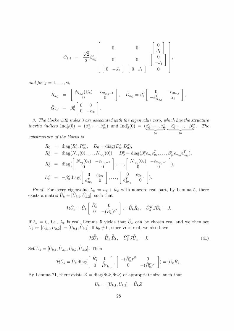
3. The blocks with index 0 are associated with the eigenvalue zero, which has the structureinertia indices IndeS(0) = (βe1, . . . , β

eq0

) and IndcS(0) = (βc0, . . . , βc0︸ ︷︷ ︸

r0

,−βc0, . . . ,−βc0︸ ︷︷ ︸r0

). The

substructure of the blocks is

R0 = diag(Re0, R

c0), D0 = diag(De

0, Dc0),

Re0 = diag(Nu1(0), . . . , Nuq0

(0)), De0 = diag(βe1eu1e

Tu1, . . . , βeq0euq0e

Tuq0

),

Rc0 = diag(

[Nv1(02) −e2v1−1

0 0

], . . . ,

[Nvr0

(02) −e2vr0−1

0 0

]),

Dc0 = −βc0 diag(

[0 e2v1

eT2v10

], . . . ,

[0 e2vr0

eT2vr0 0

]).

Proof. For every eigenvalue λk := ak + ibk with nonzero real part, by Lemma 5, thereexists a matrix Uk = [Uk,1, Uk,2], such that

HUk = Uk

[Rrk 0

0 −(Rrk)H

]:= UkRk, UH

k JUk = J.

If bk = 0, i.e., λk is real, Lemma 5 yields that Uk can be chosen real and we then setUk := [Uk,1, Uk,2] := [Uk,1, Uk,2]. If bk 6= 0, since H is real, we also have

H ¯Uk =

¯Uk

¯Rk, UT

k J¯Uk = J. (41)

Set Uk = [Uk,1,¯Uk,1, Uk,2,

¯Uk,2]. Then

HUk = Uk diag(

[Rrk 0

0¯Rr

k

],

[−(Rr

k)H 0

0 −(Rrk)T

]) =: UkRk.

By Lemma 21, there exists Z = diag(ΨΦ,ΨΦ) of appropriate size, such that

Uk := [Uk,1, Uk,2] = UkZ

28

and Rk := Z−1RkZ =:

[Rrk 0

0 −(Rrk)T

]are both real and Rr

k is in the block form described

in (40). It remains to prove that UTk JUk = J . From (41) we get that the columns of JH

¯Uk,1,

JH¯Uk,2 form the left invariant subspaces corresponding to −λk, and λk, respectively. Since

the four eigenvalues λk, λk, −λk and −λk are pairwise distinct, we get UTk,jJUk,l = 0 for

j, l = 1, 2, i.e., UTk JUk = 0. Using this fact and that UH

k JUk = J , we obtain UHk JUk = J .

Note that Z is symplectic and since Uk is real, we obtain UTk JUk = J . Setting

U := [U1, U2] = [U1,1, . . . , Uµ,1, U1,2, . . . , Uµ,2],

we have that U is real, UTJU = J and HU = U

[Rr 00 −RT

r

].

Since H is real, it follows for the blocks in

[Re De

0 −RTe

]and

[Rc Dc

0 −RTc

]correspond-

ing to the nonzero purely imaginary eigenvalues iα1, . . . , iαν that also −iα1, . . . ,−iαν areeigenvalues of H. For any block associated with an eigenvalue iαk let Vk be such that

V Hk JVk = J, HVk = Vk

[Rk Dk

0 −RHk

]= VkR,

where R contains the Jordan blocks corresponding to IndeS(iαk) and IndcS(iαk). Conjugat-ing this equation we obtain the analogous equation for −iα. Using again Lemma 21, asbefore, we obtain a real matrix V = [V1, V2], such that V TJV = J and

HV = V

Re 0 De 00 Rc 0 Dc

0 0 −RTe 0

0 0 0 −RTc

.

The next step will be the construction of a real matrix W = [W1,W2], such that

W TJW = J and HW = W

[Rd Dd

Gd −RTd

]. Unlike the complex case we have some re-

strictions on how to group the matrix pairs, which affects the choice of the couples cor-responding to IndcS(iα). Note that since H is real, if (πP2r+1, N2r+1(iα)) is a matrix pairwith the corresponding index (−1)riπ = β ∈ InddS(iα), then (πP2r+1, N2r+1(−iα)) is amatrix pair with −β ∈ InddS(−iα). Let X = [X1, X2, X3], where X1, X3 have r columnsand X2 is a vector, such that HX = XN2r+1(iα) and XHJX = πP2r+1. Set X = [X, X],Pc := diag(πP2r+1, πP2r+1), Nc := diag(N2r+1(iα), N2r+1(−iα)). Then by Lemma 16

ϕc(Pc, Nc) =: (ZHc PcZc, Z

−1c NcZc)

29

=

J2r+1,

Nr(iα) 0 −√

22er 0 0 i

√2

2βer

0 Nr(−iα) −√

22er 0 0 −i

√2

2βer

0 0 0 −i√

22βeHr i

√2

2βeHr βα

0 0 0 −Nr(iα)H 0 00 0 0 0 −Nr(−iα)H 0

0 0 −βα√

22eHr

√2

2eHr 0

,

andXZc = [X1, X1,−

√2 ReX2, Y3, Y3,−β

√2 ImX2],

where Y3 = X3(πPr)−1. Let Z = diag(Ψ2rΦ2r, 1,Ψ2rΦ2r, 1) and Σ =

[0 α−α 0

]. By

Lemma 21 we have that ZHZHc PcZcZ = J and

Z−1Z−1c NcZcZ =

Nr(Σ) −e2r−1 0 −βe2r

0 0 −βeT2r βα0 0 −Nr(Σ)T 00 −βα eT2r−1 0

is real. Furthermore X := XZcZ is also real and XTJX = J . By properly arranging thecolumns we obtain a real matrix W = [W1,W2] such that W TJW = J and

HW = W

[Rd Dd

Gd −RTd

].

Note that this construction is also valid for α = 0, since ZHc PcZc = J implies that the

columns of X and X are linearly independent, i.e., if H has a Jordan block N2r+1(0) with achain of principal vectors given by the columns of the matrix X, it must have an additionalJordan block of the same size with a chain of principal vectors given by the columns X.

For even size Jordan blocks corresponding to the eigenvalue 0 we still need to find a real

matrix V0 with V T0 JV0 = J and HV0 = V0

[Re

0 De0

0 −(Re0)T

]. Such a matrix is obtained via

Lemma 13 and ρe in Lemma 15 by initially choosing a real chains of principal vectors. Hence

there also exists a matrix V0 = [V 01 , V

02 ], such that V T

0 JV0 = J andHV0 = V0

[R0 D0

0 −RT0

].

Setting U = [U1, V1, V0

1 ,W1, U2, V2, V0

2 ,W2], it follows by Proposition 2 that U is realsymplectic and we have obtained (40).

Note that for a given Hamiltonian matrix not all types of blocks associated with a purelyimaginary have to appear in the forms (37) and (40). We clearly allow all the occurringblocks to have dimension zero in which case the associated structure inertia index is void,too.

Remark 4 Usually the terminology canonical form refers to a form which displays allthe invariants of an equivalence relation, is essentially unique, and gives the most simple

30

representative of every equivalence class. A typical example is the Jordan canonical formwhich is the canonical form under similarity. If we use plain similarity then the classicalJordan canonical form is also the canonical form for Hamiltonian matrices. But it usuallydoes not represent a Hamiltonian matrix again. Thus we have derived the forms (37) and(40) which are condensed forms under symplectic similarity. They are more complicatedthan the classical Jordan canonical forms and they are not really canonical in the usualsense, since there is some nonuniqueness in the combination of blocks in the constructionof those parts with index c and d. However, all the eigenvalues, the number of blocks andthe block sizes and also the structure inertia indices are displayed. But, since the matrix isnot block diagonal, not all eigenvectores and principal vectors are displayed directly. Fromevery classical Jordan block only half of the principal vectors can be obtained directly fromthe transformation matrix, but the remaining ones are easily constructed. We neverthelesscall (37) and (40) Hamiltonian Jordan canonical forms.

Remark 5 The eigenvalue 0 leads to some further nonuniqueness for a real Hamiltonianmatrix. There are many different ways to couple the odd size Jordan blocks correspondingto IndcS(0). When coming from the complex case and treating 0 as a complex purelyimaginary eigenvalue, we have obtained the real form from a coupling of matrix pairs(πP2r+1, N2r+1) and (−πP2r+1, N2r+1). But we can also use different combinations andthe transformations ϕ1 or ϕ2 to get a real form. Using ϕ1 (or ϕ2) for above coupledmatrix pairs the final Hamiltonian structure would be diag(N2vk+1,−NT

2vk+1) which lookssomewhat simpler than what we have given in the Theorem.

As we have already discussed in the introduction we are interested in Hamiltonian trian-gular forms under symplectic similarity transformations, since from these we can read offthe eigenvalues and the associated Lagrangian invariant subspaces. We will now presentnecessary and sufficient conditions for the existence of Hamiltonian triangular forms. Insome situations, where such triangular forms do not exist, there exist Hamiltonian trian-gular forms under nonsymplectic similarity transformations. We will also give necessaryand sufficient conditions for this case. Our first two results give necessary and sufficientconditions for the existence of Hamiltonian triangular forms. The equivalence of parts ii)and iii) in the following two theorems was first stated and proved in [17]. Here they areobtained as simple corollaries of our canonical forms.

Theorem 23 (Hamiltonian triangular Jordan canonical form)Let H be a complex Hamiltonian matrix, let iα1, . . . , iαν be its pairwise disjoint purely

imaginary eigenvalues and let the columns of Uk, k = 1, . . . , ν, span the associated invariantsubspaces. Then the following are equivalent.

i) There exists a symplectic matrix U , such that U−1HU is Hamiltonian triangular.

ii) There exists a unitary symplectic matrix U , such that UHHU is Hamiltonian trian-gular.

iii) UHk JUk is congruent to J for all k = 1, . . . , ν.

31

iv) InddS(iαk) is void for all k = 1, . . . , ν.

Moreover, if any of the equivalent conditions holds, then the symplectic matrix U can bechosen such that U−1HU is in Hamiltonian triangular Jordan canonical form

Rr 0 0 0 0 00 Re 0 0 De 00 0 Rc 0 0 Dc

0 0 0 −RHr 0 0

0 0 0 0 −RHe 0

0 0 0 0 0 −RHc

, (42)

where the blocks are defined as in (37).

Proof. i) ⇒ ii) follows directly from Lemma 3. ii) ⇒ iii) follows from Proposition 3.iii) ⇒ iv) follows from the relation between the inertia index of UH

k JUk and the structureinertia index IndS(iαk) discussed in the proof of Theorem 20. iv) ⇒ i) follows directlyfrom Theorem 20.

We also have the analogous result for the real case.

Theorem 24 (Real Hamiltonian triangular Jordan canonical form)Let H be a real Hamiltonian matrix, let iα1, . . . , iαν be its pairwise distinct nonzero purely

imaginary eigenvalues and let Uk, k = 1, . . . , ν, be the associated invariant subspaces. Thenthe following are equivalent.

i) There exists a real symplectic matrix U such that U−1HU is real Hamiltonian trian-gular.

ii) There exists a real orthogonal symplectic matrix U such that UTHU is real Hamilto-nian triangular.

iii) UHk JUk is congruent to J for all k = 1, . . . , ν.

iv) InddS(iαk) is void for all k = 1, . . . , ν.

Moreover, if any of the equivalent conditions holds, then the real symplectic matrix U canbe chosen so that U−1HU is in real Hamiltonian triangular Jordan canonical form

Rr 0 0 0 0 0 0 00 Re 0 0 0 De 0 00 0 Rc 0 0 0 Dc 00 0 0 R0 0 0 0 D0

0 0 0 0 −RTr 0 0 0

0 0 0 0 0 −RTe 0 0

0 0 0 0 0 0 −RTc 0

0 0 0 0 0 0 0 −RT0

, (43)

where the blocks are defined as in (40).

32

Proof. The proof is analogous to the proof Theorem 23, using Lemma 3, Proposition 3and Theorem 22. For ii) ⇒ iii) we observe that H is orthogonal symplectically similarto a real Hamiltonian triangular form hence it is also unitary symplectically similar to acomplex Hamiltonian triangular form.

Remark 6 Using the properties of the inertia indices, conditions iii) and iv) in Theorem 23can be relaxed to hold for ν−1 purely imaginary eigenvalues. Using the fact that eigenvaluesappear in complex conjugate pairs conditions iii) and iv) in Theorem 24 can be relaxed tohold only for half the number of the nonzero purely imaginary eigenvalues.

Similar remarks hold for Hamiltonian and symplectic pencils below.

We have shown that a Hamiltonian matrix is symplectically similar to Hamiltonian tri-angular form if and only if InddS(iα) is void for all purely imaginary eigenvalues. But thereare Hamiltonian matrices for which this structure inertia index is not void and there existsa nonsymplectic similarity transformations to Hamiltonian triangular form. A simple classof such matrices are the matrices J2p. Unitary symplectic similarity transformations donot change these matrices. (Hence J2p has no Hamiltonian triangular form under symplec-tic similarity transformations.) But J2p is similar to a Hamiltonian triangular canonicalform under nonsymplectic transformations. As an example set V = [e1, e3, e2, e4], then

V HJ2V = diag(

[0 1−1 0

],

[0 1−1 0

]) is Hamiltonian triangular.

In general we have the following necessary and sufficient condition.

Theorem 25 A Hamiltonian matrix H is similar to a Hamiltonian triangular Jordancanonical form if and only if the algebraic multiplicities of all purely imaginary eigenvaluesare even.

If H is real, then it is similar to a real Hamiltonian triangular Jordan canonical formif and only if the algebraic multiplicities of all purely imaginary eigenvalues with positiveimaginary parts are even.

Proof. We prove only the complex case. The real case can be obtained from the complexcase by using the same transformations as in the proof of Theorem 22.

The necessity follows directly from the eigenvalue properties of a Hamiltonian triangularmatrix listed in Table 1. So we only need to prove the sufficiency. An eigenvalue has evenalgebraic multiplicity if and only if it has an even number of odd size Jordan blocks. Sofor a purely imaginary eigenvalue iα its even size Jordan blocks can be transformed toa Hamiltonian triangular forms with ρe, and its odd size Jordan blocks can be pairwisecoupled and then be transformed to Hamiltonian triangular forms with ϕc or ϕ1, ϕ2. For theeigenvalues with nonzero real part, by Lemma 5, we always have the Hamiltonian triangularform. With an appropriate arrangement of columns as in the proof of Theorem 20 we obtainthe Hamiltonian triangular Jordan canonical form.

Note that a similar trick was used in [17] to derive Hamiltonian triangular forms.

33

5 Hamiltonian Kronecker canonical forms

In this section we generalize the results for Hamiltonian Jordan canonical forms to thecase of Hamiltonian pencils. We always assume that the pencils we consider are regu-lar. A treatment of singular pencils is currently under investigation and is not possible inthis already very long paper. Since the pencils are assumed to be regular, the appropriatecanonical forms should be called Hamiltonian Weierstraß canonical forms, since Weierstraß[24] was the first to derive the canonical forms for regular pencils. The form for generalpencils was developed first by Kronecker [13]. Nevertheless we will call our form Hamilto-nian Kronecker canonical form in order to avoid confusion when generalizing these resultsat a later stage to singular Hamiltonian pencils.

As shown in Table 2 for a regular Hamiltonian pencil Mh − λLh we have similar sym-metries in the finite spectrum. So most of the analysis in this section has to be devoted tothe part of the canonical form associated with infinite eigenvalues.

Let us first recall the Weierstraß canonical form for regular pencils, e.g. [10]. For anarbitrary regular matrix pencilM− λL, there exist nonsingular matrices X , Y , such that[10]

Y(M− λL)X =

[H 00 I

]− λ

[I 00 N

],

where H is in Jordan canonical form and is associated with the finite eigenvalues ofM−λL.N is a nilpotent matrix in Jordan canonical form and associated with the eigenvalue infinity.If M− λL is Hamiltonian, i.e., MJLH = −LJMH , then we obtain[

H 00 I

]K[I 00 NH

]= −

[I 00 N

]K[HH 00 I

],

where K = X−1JX−H . If we partition K conformally as a block matrix

[K1,1 K1,2

K2,1 K2,2

],

then we have

HK1,1 +K1,1HH = 0, HK1,2N

H +K1,2 = 0, K2,2NH +NK2,2 = 0.

Since N is nilpotent, from the second equation we have K1,2 = 0, see e.g., [5]. Since Kis skew Hermitian we obtain that it is block diagonal. If we partition X conformally asX = [X1, X2] then

MX1 = LX1H, MX2N = LX2, (44)

i.e., rangeX1 and rangeX2 are the deflating subspaces corresponding to the finite andinfinite eigenvalues, respectively. Moreover, since XHJX = −K−1 = − diag(K−1

1,1 , K−12,2),

we have

(XH1 JX1)H +HH(XH

1 JX1) = 0, (XH2 JX2)N +NH(XH

2 JX2) = 0.

These two equations have the same form as (9). It follows that for the eigenvalue infinity,we also have a structure inertia index IndS(∞), which can be analogously divided into

34

three parts

IndeS(∞) = (β∞,e1 , . . . , β∞,eτ ),

IndcS(∞) = (β∞,c1 , . . . , β∞,cφ ;−β∞,c1 , . . . ,−β∞,cφ ),

InddS(∞) = (β∞,d1 , . . . , β∞,dψ ), β∞,d1 = . . . = β∞,dψ (= ±1).

The analysis for the eigenvalue infinity can be carried out analogous to the analysis for thepurely imaginary finite eigenvalues. We can choose an appropriate matrix X2, such thatXH

2 JX2 is block diagonal with diagonal blocks πPr corresponding to a nilpotent matrixNr, which is one of the blocks in N .

As in matrix case there is no problem to transform the matrix pairs (πPr, Nr) correspond-ing to the indices in IndeS(∞) and IndcS(∞) to appropriate Hamiltonian triangular forms.The difficulty arises for the pairs associated with indices in InddS(∞). In order to obtaina Hamiltonian canonical form, these pairs have to be combined with pairs associated withfinite eigenvalues. Since Ind(XHJX ) has the same number of elements i and −i and sinceInd(XHJX ) consists of the elements of Ind(XH

1 JX1) followed by those of Ind(XH2 JX2),

such a coupling is always possible.For finite eigenvalues we do the reductions in the same way as in the matrix case. The de-

flating subspaces corresponding to the eigenvalues with nonzero real parts are still isotropic.So the matrix pairs that we couple with the pairs associated with the eigenvalue infinitymust have purely imaginary eigenvalues.

It follows that we obtain the following Hamiltonian Kronecker canonical form for a regularcomplex Hamiltonian pencil.

Theorem 26 (Hamiltonian Kronecker canonical form)Given a regular complex Hamiltonian pencil Mh − λLh. Then there exist a nonsingular

matrix Y and a symplectic matrix U such that

Y(Mh − λLh)U =

[M11 M12

M21 M22

]− λ

[L11 L12

L21 L22

], (45)

with

M11 − λL11 =

Rr − λIRe − λI

Rc − λIRd − λI

RM − λRL

I − λR∞

,

M21 − λL21 =

00

0Gd

GM − λGL

0

,

35

M12 − λL12 =

0De

Dc

Dd

DM − λDL

−λD∞

,

M22 − λL22 =

−RHr − λI

−RHe − λI

−RHc − λI

−RHd − λI

HM − λHL

I + λRH∞

,

and where Rr, Re, De, Rc, Dc, Rd, Dd, Gd are as in (37). The other blocks have thestructures

RM = diag(RM1 , . . . , R

Mψ ), DM = diag(DM

1 , . . . , DMψ ),

HM = diag(HM1 , . . . , HM

ψ ), GM = diag(GM1 , . . . , G

Mψ ),

RL = diag(RL1 , . . . , R

Lψ), DL = diag(DL

1 , . . . , DLψ),

HL = diag(HL1 , . . . , H

Lψ ), GL = diag(GL

1 , . . . , GLψ),

where for k = 1, . . . , ψ

RMk =

Nuk(iξk) 0 −√

22euk

Ivk 012(iξk + 1)

, DMk =

√2

2iβ∞d

0 0 −euk0 0 0

eHuk 0√

22

(iξk − 1)

,

HMk =

−Nuk(iξk)H

0 Ivk√2

2eHuk 0 1

2(iξk + 1)

, GMk = iβ∞d

0 0 00 0 00 0 −1

2(iξk − 1)

,

RLk =

Iuk 0 0

Nvk −√

22evk

12

, DLk =

√2

2iβ∞d

0 0 00 0 evk0 −eHvk

√2

2

,

HLk =

Iuk0 −NH

vk

0√

22eHvk

12

, GLk = iβ∞d

0 0 00 0 00 0 −1

2

.The remaining blocks have the structure

R∞ = diag(R∞,e, R∞,c), D∞ = diag(D∞,e, D∞,c);

R∞,e = diag(Nx1 , . . . , Nxτ ), D∞,e = diag(β∞,e1 ex1eHx1, . . . , β∞,eτ exτ e

Hxτ ),

R∞,c = diag(B∞1 , . . . , B∞φ ), D∞,c = diag(C∞1 , . . . , C

∞φ ),

36

where for k = 1, . . . , φ

B∞k =

Nyk 0 −√

22eyk

Nzk −√

22ezk

0

, C∞k = i

√2

2β∞,ck

0 0 eyk0 0 −ezk−eHyk eHzk 0

.We see that Mh − λLh has τ Kronecker blocks associated with the eigenvalue infinity cor-responding to the structure inertia indices in IndeS(∞) = (β∞,e1 , . . . , β∞,eτ ). It has 2φ Kro-necker blocks corresponding to the indices in IndcS(∞) = (β∞,c1 , . . . , β∞,cφ ,−β∞,c1 , . . . ,−β∞,cφ );

and ψ blocks corresponding to the indices in InddS(∞) = (β∞d , . . . , β∞d︸ ︷︷ ︸

ψ

). The remaining

blocks are associated with ψ purely imaginary eigenvalues iξ1, . . . , iξψ ∈ iα1, . . . , iαν.The associated matrix pair has the corresponding index in InddS(iξk) and is the part that is

left over after the coupling in

[Rd Dd

Gd −RHd

].

Proof. The analysis that we have given already covers most of the blocks. It remains toshow how we get the blocks in[

RM DM

GM HM

]− λ

[RL DL

GL HL

].

Suppose that (πP2v+1, N2v+1) is a matrix pair with the corresponding structure inertia indexβ ∈ InddS(∞). By our analysis there exists a matrix pair (π1P2u+1, N2u+1(iα)) associatedwith an index of opposite sign. For an infinite eigenvalue in the pencil case the pairsare actually (πP2v+1, I − λN2v+1) and (π1P2u+1, N2u+1(iα) − λI). A transformation onthe direct sum of these two pairs is equivalent to a congruence transformation on Pc =diag(π1P2u+1, πP2v+1) and an equivalence transformation on the pencil

Nc − λLc := diag(N2u+1(iα), I)− λ diag(I,N2v+1).

If we use the transformation ϕc, then we get that ZHc PcZc = J , Z−1

c (Nc− λLc)Zc is in thedesired form.

Remark 7 As we see from Theorem 26 the canonical form has several parts, a Hamiltoniantriangular part associated with finite eigenvalues, a Hamiltonian part, also associated withfinite eigenvalues, that cannot be made triangular by transformations with symplectic Uand nonsingular Y , a Hamiltonian triangular part associated with the eigenvalue infinity[R∞ D∞0 −RH

∞

]and one part which results from a mixture of blocks associated with finite

and infinite eigenvalues.

For a real Hamiltonian pencil the real Hamiltonian Kronecker canonical form is simpler,since there is no part resulting from mixing blocks to finite and infinite eigenvalues. The

37

reason is that in the real caseX2 as in (44), the basis of the deflating subspace correspondingto eigenvalue infinity can be chosen real, i.e., Ind(XH

2 JX2) has an equal number of elementsi and −i. So we can use the same trick that we have used to deal with zero eigenvaluesin the matrix case in the proof of Theorem 22 to get the triangular block for the infiniteeigenvalue.

Theorem 27 (Real Hamiltonian Kronecker canonical form)Given a real regular Hamiltonian pencil Mh − λLh. Then there exist a real nonsingular

matrix Y and a real symplectic matrix U , such that

Y(Mh − λLh)U =

[M11 M12

M21 M22

]− λ

[L11 L12

L21 L22

], (46)

with

M11 − λL11 =

Rr − λIRe − λI

Rc − λIR0 − λI

Rd − λII − λR∞

,

M21 − λL21 =

00

00

Gd

0

,

M12 − λL12 =

0De

Dc

D0

Dd

−λD∞

,

M22 − λL22 =

−RTr − λI

−RTe − λI

−RTc − λI

−RT0 − λI

−RTd − λI

I + λRT∞

,

and where Rr, Re, De, Rc, Dc, R0, D0, Rd, Dd, Gd are as in (40). The blocks associatedwith the eigenvalue infinity are

R∞ = diag(R∞,e, R∞,c), D∞ = diag(D∞,e, D∞,c),

38

R∞,e = diag(Nx1 , . . . , Nxτ ), D∞,e = diag(β∞,e1 ex1eTx1, . . . β∞,eτ exτ e

Txτ ),

R∞,c = diag(B∞1 , . . . , B∞φ ), D∞,c = diag(C∞1 , . . . , C

∞φ ),

where for k = 1, . . . , φ

B∞k =

Nyk(

[0 00 0

]) −e2yk−1

0 0

, C∞k = −β∞c

[0 e2yk

eT2yk 0

].

The subpencil I − λ[R∞ D∞0 −RT

∞

]is the canonical form corresponding to the eigenvalue

infinity. IndeS(∞) = (β∞,e1 , . . . , β∞,eτ ) is the structure inertia index for even size Kroneckerblocks and IndcS(∞) = (β∞c , . . . , β

∞c︸ ︷︷ ︸

φ

;−β∞c , . . . ,−β∞c︸ ︷︷ ︸φ

), is the structure inertia index for odd

size Kronecker blocks. The index InddS(∞) is void.

Proof. The proof is obtained analogous to that of Theorem 22.Analogous to the matrix case we also have necessary and sufficient conditions for the

existence of a Hamiltonian triangular Kronecker canonical form. To obtain such a form weneed the following lemma.

Lemma 28 Given a regular Hamiltonian pencilMh−λLh. Let iα1, . . . , iαν be its pairwisedistinct purely imaginary eigenvalues and let the columns of Uk span the correspondingdeflating subspaces. Let furthermore the columns of U∞ span the deflating subspace to theeigenvalue ∞. Suppose there exists a nonsingular matrix Y and a symplectic matrix Usuch that Y(Mh − λLh)U is Hamiltonian triangular. Then for all k = 1, . . . , ν, UH

k JUk iscongruent to J , and UH

∞JU∞ is also congruent to J .

Proof. By hypothesis there is a nonsingular matrix Y and a symplectic matrix U suchthat

Y(Mh − λLh)U =

[M1 M3

0 M2

]− λ

[L1 L3

0 L2

]is in Hamiltonian triangular form. Since Mh − λLh is regular, M1 − λL1 and M2 − λL2

are both regular. For the first subpencil there exist nonsingular Y1 and Z1 so that

Y1(M1 − λL1)Z1 =

[A 00 I

]− λ

[I 00 B

]

is in Kronecker canonical form. Let X1 be nonsingular, such that X1M2Z−H1 is lower

triangular, (this is a QL factorization, see [11]), and set Y1 = diag(Y1, X1)Y , U1 =U diag(Z1, Z

−H1 ). Then U1 is symplectic and

Y1(M− λL)U1 =

A 0 M1,3 M1,4

0 I M2,3 M2,4

0 0 M3,3 00 0 M4,3 M4,4

− λI 0 L1,3 L1,4

0 B L2,3 L2,4

0 0 L3,3 L3,4

0 0 L4,3 L4,4

.

39

Using the Hamiltonian property, we get[A 00 I

] [L3,3 L3,4

L4,3 L4,4

]H+

[I 00 B

] [M3,3 0M4,3 M4,4

]H= 0.

Comparing the blocks on both sides, we have L3,4 = 0, and

ALH3,3 +MH3,3 = 0, LH4,4 +BMH

4,4 = 0, ALH4,3 +MH4,3 = 0. (47)

By the regularity of the pencil L3,3, M4,4 must be nonsingular. Set

Y2 = diag(I,

[L−1

3,3 0−M−1

4,4L4,3L−13,3 M−1

4,4

])Y1,

then by (47) it follows that

Y2(M− λL)U1 =

A 0 M1,3 M1,4

0 I M2,3 M2,4

0 0 −AH 00 0 0 I

− λI 0 L1,3 L1,4

0 B L2,3 L2,4

0 0 I 00 0 0 −BH

.

Since B is nilpotent Λ(B, I) ∩ Λ(I,−AH) = ∅. So the matrix equation

BX + Y = L2,3, X − Y AH = M2,3

has unique solutions X2, Y2, see [5].Set

Y3 =

I 0 0 AXH

2 −M1,4

0 I −Y2 00 0 I 00 0 0 I

Y2, U = U1

I 0 0 −XH

2

0 I −X2 00 0 I 00 0 0 I

.

Then U2 is symplectic and we can easily verify that

Y3(M− λL)U =

A 0 M1,3 00 I 0 M2,4

0 0 −AH 00 0 0 I

− λI 0 L1,3 00 B 0 L2,4

0 0 I 00 0 0 −BH

.

Finally setting

Y =

I 0 −L1,3 00 I 0 −M2,4

0 0 I 00 0 0 I

Y3,

40

we obtain

Y(M− λL)U =

A 0 DA 00 I 0 00 0 −AH 00 0 0 I

− λI 0 0 00 B 0 DB

0 0 I 00 0 0 −BH

.and clearly DA, DB are Hermitian.

PartitionU = [U1,1, U1,2, U2,1, U2,2 ]

conformally. Then V1 = [U1,1, U2,1 ] and V2 = [U1,2, U2,2 ] are the bases of the deflatingsubspaces corresponding to the finite eigenvalues and eigenvalue infinity, respectively. SinceU is symplectic, V H

k JVk = J for k = 1, 2. Moreover,

MhV1 = LhV1

[A DA

0 −AH]

=: LhV1HA, MhV2HB :=MhV2

[B DB

0 −BH

]= LhV2.

Since HA is Hamiltonian triangular, by Proposition 3 and V H1 JV1 = J we have that

UHk JUk is congruent to J for all k = 1, . . . , ν. Since HB is also Hamiltonian triangular and

nilpotent, by exchanging the roles ofMh and Lh in the pencil we get that UH∞JU∞ is also

congruent to J .

Theorem 29 (Hamiltonian triangular Kronecker canonical form)Let Mh − λLh be a regular complex Hamiltonian pencil , let iα1, . . . , iαν be its pairwise

distinct purely imaginary eigenvalues and let the columns of Uk span the correspondingdeflating subspaces. Let furthermore the columns of U∞ span the deflating subspace to theeigenvalue ∞. Then the following are equivalent.

i) There exist a nonsingular matrix Y and a symplectic matrix U such that Y(Mh −λLh)U is Hamiltonian triangular.

ii) There exist a unitary matrix Y and a unitary symplectic matrix U such that Y(Mh−λLh)U is Hamiltonian triangular.

iii) For all k = 1, . . . , ν, UHk JUk is congruent to J and UH

∞JU∞ is also congruent to J .

iv) For all k = 1, . . . , ν the structure inertia indices InddS(iαk) and InddS(∞) are void.

Moreover, if any of the equivalent conditions holds, then the matrices Y, U can be chosenso that Y(Mh − λLh)U is in Hamiltonian triangular Kronecker canonical form

Rr − λI 0Re − λI De

Rc − λI Dc

I − λR∞ −λD∞0 −RH

r − λI0 −RH

e − λI0 −RH

c − λI0 I + λRH

∞

,

41

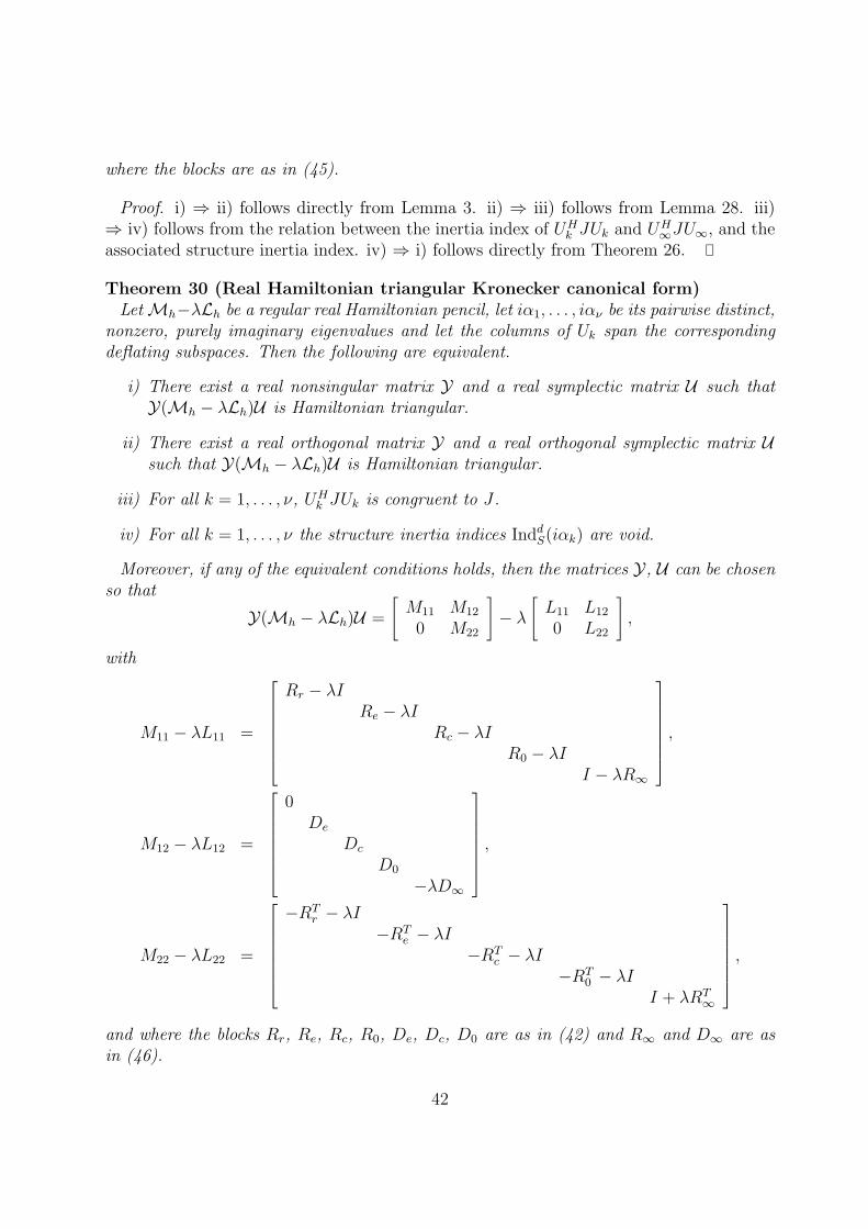
where the blocks are as in (45).

Proof. i) ⇒ ii) follows directly from Lemma 3. ii) ⇒ iii) follows from Lemma 28. iii)⇒ iv) follows from the relation between the inertia index of UH

k JUk and UH∞JU∞, and the

associated structure inertia index. iv) ⇒ i) follows directly from Theorem 26.

Theorem 30 (Real Hamiltonian triangular Kronecker canonical form)LetMh−λLh be a regular real Hamiltonian pencil, let iα1, . . . , iαν be its pairwise distinct,

nonzero, purely imaginary eigenvalues and let the columns of Uk span the correspondingdeflating subspaces. Then the following are equivalent.

i) There exist a real nonsingular matrix Y and a real symplectic matrix U such thatY(Mh − λLh)U is Hamiltonian triangular.

ii) There exist a real orthogonal matrix Y and a real orthogonal symplectic matrix Usuch that Y(Mh − λLh)U is Hamiltonian triangular.

iii) For all k = 1, . . . , ν, UHk JUk is congruent to J .

iv) For all k = 1, . . . , ν the structure inertia indices InddS(iαk) are void.

Moreover, if any of the equivalent conditions holds, then the matrices Y, U can be chosenso that

Y(Mh − λLh)U =

[M11 M12

0 M22

]− λ

[L11 L12

0 L22

],

with

M11 − λL11 =

Rr − λI

Re − λIRc − λI

R0 − λII − λR∞

,

M12 − λL12 =

0

De

Dc

D0

−λD∞

,

M22 − λL22 =

−RT

r − λI−RT

e − λI−RT

c − λI−RT

0 − λII + λRT

∞

,

and where the blocks Rr, Re, Rc, R0, De, Dc, D0 are as in (42) and R∞ and D∞ are asin (46).

42

Proof. The proof is similar to the proof of Theorem 29, using Lemma 3, Lemma 28 andTheorem 27.

We also have the corresponding result on the Hamiltonian triangular Kronecker canonicalform under nonsymplectic transformations.

Theorem 31 A regular Hamiltonian pencil Mh−λLh has a Hamiltonian triangular Kro-necker canonical form if and only if the algebraic multiplicities of all purely imaginaryeigenvalues are even.

If Mh − λLh is real it has a real Hamiltonian triangular Kronecker canonical form ifand only if the algebraic multiplicities of all purely imaginary eigenvalues with positiveimaginary parts are even.

Proof. The proof is similar to the proof of Theorem 25. Note that the condition that allfinite eigenvalues have even algebraic multiplicities implies that the algebraic multiplicityfor the eigenvalue infinity is also even. The canonical form for the infinite eigenvalue canbe constructed in the same way as that for the eigenvalue zero by exchanging the roles ofLh and Mh.

In this section we have shown that there exist canonical forms analogous to the matrixcase for Hamiltonian pencils. In the next sections we will use the generalized Cayleytransformation, to obtain similar results also for symplectic matrices and pencils.

6 Technical lemmas for the symplectic case

In this section we now present some technical results that are needed to derive the canonicalforms for symplectic pencils. The first tool that we will make use of is a generalization ofthe Cayley transformation, see [19].

Proposition 5 A matrix pencil Mh − λLh is Hamiltonian if and only if the pencil

χ(Mh − λLh) := (Mh + Lh)− λ(Mh − Lh) =:Ms − λLs

is symplectic. Mh − λLh is regular if and only if Ms − λLs is regular.

The generalized Cayley transformation relates the spectrum of a Hamiltonian pencil Λ(Mh,Lh)and the spectrum of the associated symplectic pencilMs − λLs as shown in Table 5. Thestructure of the associated Jordan blocks and deflating subspaces, however, is not alteredby the generalized Cayley transformation, since for any matrix pencil A − λB we haveχ(Y (A− λB)U) = Y (χ(A− λB))U .

We may apply the generalized Cayley transformation directly to the canonical forms (45)and (46) and we will obtain an analogous block structure. Unfortunately the Cayley trans-formation does not produce a form that is as condensed, so some further transformationsare needed. To do this construction we need some more technical lemmas.

43

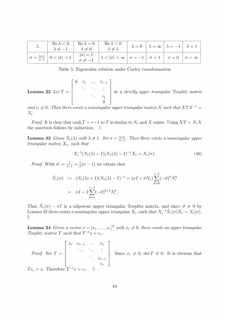
λReλ < 0λ 6= −1

Reλ = 0λ 6= 0

Reλ > 0λ 6= 1

λ = 0 λ =∞ λ = −1 λ = 1

σ = λ+1λ−1

0 < |σ| < 1|σ| = 1σ 6= −1

1 < |σ| <∞ σ = −1 σ = 1 σ = 0 σ =∞

Table 5: Eigenvalue relation under Cayley transformation

Lemma 32 Let T =

0 τ1 . . . τr−1

. . . . . ....

. . . τ1

0

be a strictly upper triangular Toeplitz matrix

and τ1 6= 0. Then there exists a nonsingular upper triangular matrix X such that XTX−1 =Nr.

Proof. It is clear that rankT = r−1 so T is similar to Nr and X exists. Using XT = NrXthe assertion follows by induction.

Lemma 33 Given Nr(λ) with λ 6= 1. Set σ = λ+1λ−1

. Then there exists a nonsingular uppertriangular matrix Xr, such that

X−1r (Nr(λ) + I)(Nr(λ)− I)−1Xr = Nr(σ). (48)

Proof. With ϑ := 1λ−1

= 12(σ − 1) we obtain that

Nr(σ) := (Nr(λ) + I)(Nr(λ)− I)−1 = (σI + ϑNr)r−1∑k=0

(−ϑ)kNkr

= σI − 2r−1∑k=1

(−ϑ)k+1Nkr .

Thus Nr(σ) − σI is a nilpotent upper triangular Toeplitz matrix, and since ϑ 6= 0 byLemma 32 there exists a nonsingular upper triangular Xr, such that X−1

r Nr(σ)Xr = Nr(σ).

Lemma 34 Given a vector x = [x1, . . . , xr]T with xr 6= 0, there exists an upper triangular

Toeplitz matrix T such that T−1x = er.

Proof. Set T =

xr xr−1 . . . x1

. . . . . ....

. . . xr−1

xr

. Since xr 6= 0, detT 6= 0. It is obvious that

Ter = x. Therefore T−1x = er.

44

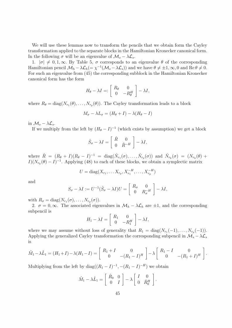
We will use these lemmas now to transform the pencils that we obtain form the Cayleytransformation applied to the separate blocks in the Hamiltonian Kronecker canonical form.In the following σ will be an eigenvalue of Ms − λLs.

1. |σ| 6= 0, 1,∞. By Table 5, σ corresponds to an eigenvalue θ of the correspondingHamiltonian pencilMh−λLh(= χ−1(Ms−λLs)) and we have θ 6= ±1,∞, 0 and Re θ 6= 0.For such an eigenvalue from (45) the corresponding subblock in the Hamiltonian Kroneckercanonical form has the form

Hθ − λI =:

[Rθ 00 −RH

θ

]− λI,

where Rθ = diag(Nr1(θ), . . . , Nrp(θ)). The Cayley transformation leads to a block

Mσ − λLσ = (Hθ + I)− λ(Hθ − I)

in Ms − λLs.If we multiply from the left by (Hθ − I)−1 (which exists by assumption) we get a block

Sσ − λI =

[R 0

0 R−H

]− λI,

where R = (Rθ + I)(Rθ − I)−1 = diag(Nr1(σ), . . . , Nrp(σ)) and Nrk(σ) = (Nrk(θ) +I)(Nrk(θ)− I)−1. Applying (48) to each of these blocks, we obtain a symplectic matrix

U = diag(Xr1 , . . . Xrp , X−Hr1

, . . . , X−Hrp )

and

Sσ − λI := U−1(Sσ − λI)U =

[Rσ 00 R−Hσ

]− λI,

with Rσ = diag(Nr1(σ), . . . , Nrp(σ)).2. σ = 0,∞. The associated eigenvalues in Mh − λLh are ±1, and the corresponding

subpencil is

H1 − λI =

[R1 00 −RH

1

]− λI,

where we may assume without loss of generality that R1 = diag(Nr1(−1), . . . , Nrp(−1)).Applying the generalized Cayley transformation the corresponding subpencil inMs−λLsis

M1−λL1 = (H1 +I)−λ(H1−I) =

[R1 + I 0

0 −(R1 − I)H

]−λ

[R1 − I 0

0 −(R1 + I)H

].

Multiplying from the left by diag((R1 − I)−1,−(R1 − I)−H) we obtain

M1 − λL1 =

[R0 00 I

]− λ

[I 0

0 RH0

].

45

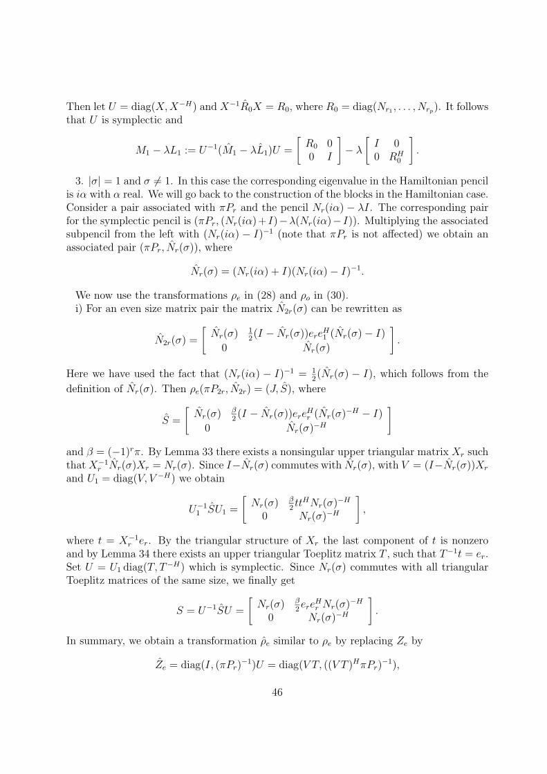
Then let U = diag(X,X−H) and X−1R0X = R0, where R0 = diag(Nr1 , . . . , Nrp). It followsthat U is symplectic and

M1 − λL1 := U−1(M1 − λL1)U =

[R0 00 I

]− λ

[I 00 RH

0

].

3. |σ| = 1 and σ 6= 1. In this case the corresponding eigenvalue in the Hamiltonian pencilis iα with α real. We will go back to the construction of the blocks in the Hamiltonian case.Consider a pair associated with πPr and the pencil Nr(iα) − λI. The corresponding pairfor the symplectic pencil is (πPr, (Nr(iα)+ I)−λ(Nr(iα)− I)). Multiplying the associatedsubpencil from the left with (Nr(iα) − I)−1 (note that πPr is not affected) we obtain anassociated pair (πPr, Nr(σ)), where

Nr(σ) = (Nr(iα) + I)(Nr(iα)− I)−1.

We now use the transformations ρe in (28) and ρo in (30).i) For an even size matrix pair the matrix N2r(σ) can be rewritten as

N2r(σ) =

[Nr(σ) 1

2(I − Nr(σ))ere

H1 (Nr(σ)− I)

0 Nr(σ)

].

Here we have used the fact that (Nr(iα) − I)−1 = 12(Nr(σ) − I), which follows from the

definition of Nr(σ). Then ρe(πP2r, N2r) = (J, S), where

S =

[Nr(σ) β

2(I − Nr(σ))ere

Hr (Nr(σ)−H − I)

0 Nr(σ)−H

]

and β = (−1)rπ. By Lemma 33 there exists a nonsingular upper triangular matrix Xr suchthat X−1

r Nr(σ)Xr = Nr(σ). Since I−Nr(σ) commutes with Nr(σ), with V = (I−Nr(σ))Xr

and U1 = diag(V, V −H) we obtain

U−11 SU1 =

[Nr(σ) β

2ttHNr(σ)−H

0 Nr(σ)−H

],

where t = X−1r er. By the triangular structure of Xr the last component of t is nonzero

and by Lemma 34 there exists an upper triangular Toeplitz matrix T , such that T−1t = er.Set U = U1 diag(T, T−H) which is symplectic. Since Nr(σ) commutes with all triangularToeplitz matrices of the same size, we finally get

S = U−1SU =

[Nr(σ) β

2ere

Hr Nr(σ)−H

0 Nr(σ)−H

].

In summary, we obtain a transformation ρe similar to ρe by replacing Ze by

Ze = diag(I, (πPr)−1)U = diag(V T, ((V T )HπPr)

−1),

46

which transforms (πP2r, N2r(σ)) to (J, S).ii) For an odd sized pair (πP2r+1, N2r+1(σ)), we set V = 1−σ

2(I − Nr(σ))XrT , where Xr

and T are defined as in the even case and

Zo := diag(V, 1, (πV HPr)−1).

Then one can easily verify that

ρo(πP2r+1, N2r+1(σ)) = (ZHo (πP2r+1)Zo, Z

−1o N2r+1(σ)Zo) =

=

0 0 I

0 iβ 0−I 0 0

, Nr(σ) σer

σσ−1

iβereHr Nr(σ)−H

0 σ iβeHr Nr(σ)−H

0 0 Nr(σ)−H

,

where β = (−1)riπ.4. σ = 1. Then the corresponding eigenvalue in Mh − λLh is infinity and the pair is

constructed from πPr and I−λNr which leads to the pair πPr and (I +Nr)−λ(I−Nr) inMs−λLs. In matrix form the associated pair is (πPr, Nr(1)), where Nr(1) := (I+Nr)(I−Nr)

−1. (Note that the form of Nr(1) is slightly different from that of Nr(σ) for σ 6= 1).We still have a nonsingular upper triangular matrix Xr, such that X−1

r Nr(1)Xr = Nr(1).Using this Xr to replace Xr above and changing T appropriately, we get for even size pairs

ρe(πP2r, N2r(1)) =

(J,

[Nr(1) β

2ere

Hr Nr(1)−H

0 Nr(1)−H

])

which is the same as in the case σ 6= 1. For odd size pairs we obtain

ρo(πP2r+1, N2r+1(1)) =

0 0 I

0 iβ 0−I 0 0

, Nr(1) er

iβ2ere

Hr Nr(1)−H

0 1 iβeHr Nr(1)−H

0 0 Nr(1)−H

.

For even size matrix pairs the condensed form already is in symplectic triangular canon-ical form. It remains to perform a coupling for the odd size pairs. Similar to the Hamil-tonian case we construct a transformation ϕc, just using Zo instead of Zo, and apply it to(Pc, Nc), where Pc = diag(π1P2r1+1, π2P2r2+1), Nc = diag(N2r1+1(σ1), N2r2+1(σ2)) with thecorresponding β1 = −β2. Then

ϕc(Pc, Nc) =

Jr1+r2+1,

Nr1(σ1) 0 −√

22σ1er1

0 Nr2(σ2) −√

22σ2er2

0 0 12(σ1 + σ2)

0 0 00 0 0

0 0 iβ1

2(σ1 − σ2)

47

iβ1f(σ1)er1eHr1Nr1(σ1)−H 0

√2

2iβ1σ1er1

0 −iβ1f(σ2)er2eHr2Nr2(σ2)−H −

√2

2iβ1σ2er2

−√

22iβ1e

Hr1Nr1(σ1)−H

√2

2iβ1e

Hr2Nr2(σ2)−H − iβ1

2(σ1 − σ2)

Nr1(σ1)−H 0 00 Nr2(σ2)−H 0√

22eHr1Nr1(σ1)−H

√2

2eHr2Nr2(σ2)−H 1

2(σ1 + σ2)

,

where

f(σ) =σ

σ − 1for |σ| = 1, σ 6= 1; f(1) =

1

2. (49)

7 Symplectic Kronecker canonical forms

Using these basic technical results and the obtained matrix block forms we can now as-semble the symplectic Kronecker canonical form.

Theorem 35 (Symplectic Kronecker canonical form) Given a regular complex sym-plectic pencil Ms−λLs. Then there exist a nonsingular matrix Y and a symplectic matrixU such that

Y(Ms − λLs)U =

[M11 M12

M21 M22

]− λ

[L11 L12

L21 L22

], (50)

with

M11 − λL11 =

Rr − λI

Re − λIRc − λI

Rd − λIR0 − λI

,

M21 − λL21 =

0

00

Gd

0

,

M12 − λL12 =

0

De

Dc

Dd

0

,

M22 − λL22 =

R−Hr − λI

R−He − λIR−Hc − λI

Sd − λII − λRH

0

,

48

where the blocks are as follows.1. The blocks with index r are associated with the pairwise distinct eigenvalues σ1, . . . , σµ,

σ−11 , . . . , σ−1

µ , such that |σk| 6= 1. The blocks have the structure

Rr = diag(Rr1, . . . , R

rµ),

Rrk = diag(Ndk,1(σk), . . . , Ndk,pk

(σk)), k = 1, . . . , µ.

2. The blocks with indices e and c are associated with unimodular eigenvalues θ1, . . . , θν.The associated parts of the structure inertia indices are IndeS(θk) = (βek,1, . . . , β

ek,qk

), andIndcS(θk) = (βck,1, . . . , β

ck,rk

,−βck,1, . . . ,−βck,rk). The structures of the blocks are

Re = diag(Re1, . . . , R

eν), De = diag(De

1, . . . , Deν),

Rek = diag(Nlk,1(θk), . . . , Nlk,qk

(θk)),

Dek =

1

2diag(βek,1elk,1e

Hlk,1Nlk,1(θk)

−H , . . . , βek,qkelk,qkeHlk,qk

Nlk,qk(θk)

−H),

Rc = diag(Rc1, . . . , R

cν), Dc = diag(Dc

1, . . . , Dcν),

Rck = diag(Bk,1, . . . , Bk,rk), Dc

k = diag(Ck,1, . . . , Ck,rk),

where for k = 1, . . . , ν and j = 1, . . . , rk we have

Bk,j =

Nmk,j(θk) 0 −√

22θkemk,j

Nnk,j(θk) −√

22θkenk,jθk

,

Ck,j = iβck,j

f(θk)emk,je

Hmk,j

Nmk,j(θk)−H 0

√2

2θkemk,j

0 −f(θk)enk,jeHnk,j

Nnk,j(θk)−H −

√2

2θkenk,j

−√

22eHmk,jNmk,j(θk)

−H√

22eHnk,jNnk,j(θk)

−H 0

,and f(θk) is as in (49).

3. The blocks with index d are associated with two disjoint sets of unimodular eigenvaluesγ1, . . . , γη and δ1, . . . , δη with the corresponding structure inertia indices (βd1 , . . . , β

dη)

and (−βd1 , . . . ,−βdη), respectively, where βd1 = . . . = βdη . The corresponding Kroneckerblocks have the following block structures.

Rd = diag(Rd1, . . . , R

dη), Dd = diag(Dd

1, . . . , Ddη),

Sd = diag(Sd1 , . . . , Sdη), Gd = diag(Gd

1, . . . , Gdη),

where for k = 1, . . . , η we have

Rdk =

Nsk(γk) 0 −√

22γkesk

Ntk(δk) −√

22δketk

12(γk + δk)

,

49

Ddk = iβdk

f(γk)eske

HskNsk(γk)

−H 0√

22γkesk

0 −f(δk)etkeHtkNtk(δk)

−H −√

22δketk

−√

22eHskNsk(γk)

−H√

22eHtkNtk(δk)

−H −12(γk − δk)

,

Sdk =

Nsk(γk)−H

0 Ntk(δk)−H

√2

2eHskNsk(γk)

−H√

22eHtkNtk(δk)

−H 12(γk + δk)

,

Gdk = iβdk

0 0 00 0 00 0 1

2(γk − δk)

.4. The blocks with index 0 are associated with zero and infinite eigenvalues and have the

structureR0 = diag(Nz1 , . . . , Nzτ ).

Proof. Using the above construction, the proof follows from the Hamiltonian case.Again analogous to the Hamiltonian case, we have a result for real symplectic pencils. We

use the following notation. Either Σk =

[σk,1 σk,2−σk,2 σk,1

], with σk,2 6= 0 and σ2

k,1 + σ2k,2 6= 1,

or Σk is a real number and Σk 6= ±1. Blocks ∆k have the form

[ak bk−bk ak

], a2

k + b2k = 1

and ak 6= 1. Furthermore we have blocks F (∆k) = 12

[fk 1−1 fk

]with fk = bk

1−ak, and

F (I2) = 12J1.

Theorem 36 (Real symplectic Kronecker canonical form) Given a real regular sym-plectic pencilMs−λLs. Then there exist a real nonsingular matrix Y and a real symplecticmatrix U such that

Y(Ms − λLs)U =

[M11 M12

M21 M22

]− λ

[L11 L12

L21 L22

], (51)

with

M11 − λL11 =

Rr − λIRe − λI

Rc − λIRu − λI

Rd − λIR0 − λI

,

M21 − λL21 =

00

00

Gd

0

,

50

M12 − λL12 =

0De

Dc

Du

Dd

0

,

M22 − λL22 =

R−Tr − λIR−Te − λI

R−Tc − λIR−Tu − λI

Sd − λII − λRT

0

,

and where we have the following structure for the different blocks.1. If Σk is a nonzero real number, Σk and Σ−1

k are both real eigenvalues of Ms−λLs. Ifσk,2 6= 0, then σk = σk,1 +iσk,2, together with σk, σ−1

k , and σ−1k are eigenvalues ofMs−λLs

and the associated blocks have the structure

Rr = diag(Rr1, . . . , R

rµ),

Rrk = diag(Ndk,1(Σk), . . . , Ndk,pk

(Σk)),

2. The blocks with indices c, e and d are associated with unimodular eigenvalues θk :=

ak + ibk and θk contained in ∆k =

[ak bk−bk ak

]with θk 6= ±1. The associated structure

inertia indices are

IndeS(θk) = (βek,1, . . . , βek,qk

),

IndcS(θk) = (βck,1, . . . , βck,rk

,−βck,1, . . . ,−βck,rk),InddS(θk) = (βdk , . . . , β

dk︸ ︷︷ ︸

sk

),

IndeS(θk) = (βek,1, . . . , βek,qk

),

IndcS(θk) = (−βck,1, . . . ,−βck,rk , βck,1, . . . , β

ck,rk

),

InddS(θk) = (−βdk , . . . ,−βdk︸ ︷︷ ︸sk

),

and the blocks have the following form.

Re = diag(Re1, . . . , R

eν), De = diag(De

1, . . . , Deν),

Rc = diag(Rc1, . . . , R

cν), Dc = diag(Dc

1, . . . , Dcν),

where for k = 1, . . . , ν,

Rek = diag(Nlk,1(∆k), . . . , Nlk,qk

(∆k)),

51

Dek =

1

2diag(βek,1

[0 00 I2

]Nlk,1(∆k)

−T , . . . , βek,qk

[0 00 I2

]Nlk,qk

(∆k)−T ),

Rck = diag(Bk,1, . . . , Bk,rk), Dc

k = diag(Ck,1, . . . , Ck,rk),

and for k = 1, . . . , ν, j = 1, . . . , rk

Bk,j =

Nmk,j(∆k) 0

[0

−√

22

∆k

]

Nnk,j(∆k)

[0

−√

22

∆k

]0 0 ∆k

,

Ck,j = βck,j

[0 00 F (∆k)

]Nmk,j(∆k)

−T 0

[0√

22J1∆k

]

0 −[

0 00 F (∆k)

]Nnk,j(∆k)

−T[

0

−√

22J1∆k

][

0 −√

22J1

]Nmk,j(∆k)

−T[

0√

22J1

]Nnk,j(∆k)

−T 0

.

The blocks with index d have the form

Rd = diag(Rd1, . . . , R

dν), Dd = diag(Dd

1, . . . , Ddν),

Sd = diag(Sd1 , . . . , Sdν ), Gd = diag(Gd

1, . . . , Gdν),

Rdk = diag(Tk,1, . . . , Tk,sk), Dd

k = diag(Xk,1, . . . , Xk,sk),

Sdk = diag(Zk,1, . . . , Zk,sk), Gdk = diag(Yk,1, . . . , Yk,sk),

where for k = 0, 1, . . . , ν, j = 1, . . . , sk

Tk,j =

Ntk,j(∆k)

0−akbk

0 ak

, Xk,j = βdk

[

0 00 F (∆k)

]Ntk,j(∆k)

−T

0−bk−ak

−eT2tk,jNtk,j(∆k)

−T bk

,

Zk,j =

[Ntk,j(∆)−T 0

eT2tk,j−1Ntk,j(∆k)−T ak

], Yk,j = βdk

[0 00 −bk

].

3. The blocks with index u are associated with the eigenvalues ±1. In particular theblocks with index + are associated with the eigenvalue 1. Here InddS(1) is void and theother structure inertia indices are

IndeS(1) = (βe+1 , . . . , βe+q+ ), IndcS(1) = (βc+, . . . , βc+︸ ︷︷ ︸

r+

,−βc+, . . . ,−βc+︸ ︷︷ ︸r+

).

The blocks with index − are associated with the eigenvalue −1. Here InddS(−1) is void andthe other structure inertia indices are

IndeS(−1) = (βe−1 , . . . , βe−q− ), IndcS(−1) = (βc−, . . . , βc−︸ ︷︷ ︸

r−

,−βx−, . . . ,−βc−︸ ︷︷ ︸r−

).

52

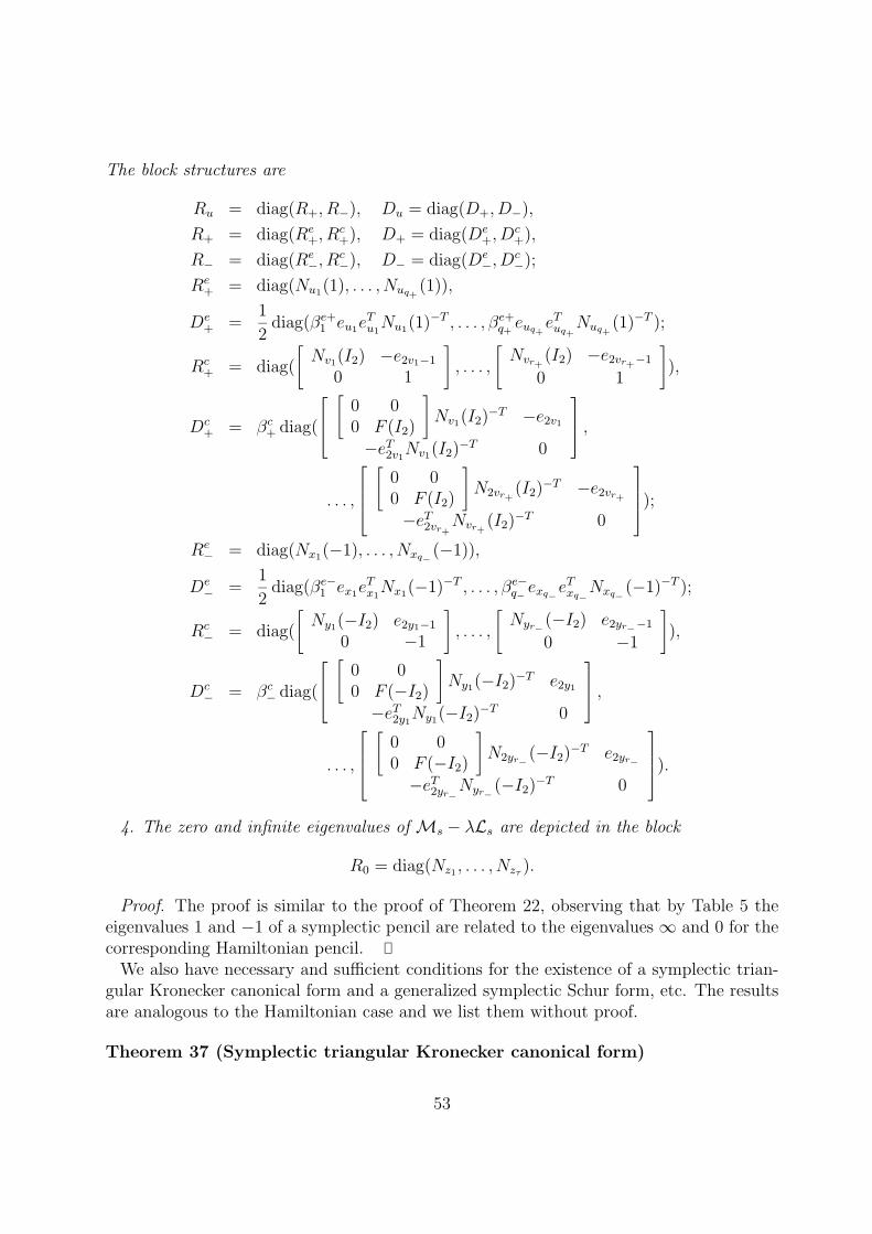
The block structures are

Ru = diag(R+, R−), Du = diag(D+, D−),

R+ = diag(Re+, R

c+), D+ = diag(De

+, Dc+),

R− = diag(Re−, R

c−), D− = diag(De

−, Dc−);

Re+ = diag(Nu1(1), . . . , Nuq+

(1)),

De+ =

1

2diag(βe+1 eu1e

Tu1Nu1(1)−T , . . . , βe+q+ euq+e

Tuq+

Nuq+(1)−T );

Rc+ = diag(

[Nv1(I2) −e2v1−1

0 1

], . . . ,

[Nvr+

(I2) −e2vr+−1

0 1

]),

Dc+ = βc+ diag(

[

0 00 F (I2)

]Nv1(I2)−T −e2v1

−eT2v1Nv1(I2)−T 0

,

. . . ,

[

0 00 F (I2)

]N2vr+

(I2)−T −e2vr+

−eT2vr+Nvr+(I2)−T 0

);

Re− = diag(Nx1(−1), . . . , Nxq−

(−1)),

De− =

1

2diag(βe−1 ex1e

Tx1Nx1(−1)−T , . . . , βe−q− exq−e

Txq−

Nxq−(−1)−T );

Rc− = diag(

[Ny1(−I2) e2y1−1

0 −1

], . . . ,

[Nyr−

(−I2) e2yr−−1

0 −1

]),

Dc− = βc− diag(

[

0 00 F (−I2)

]Ny1(−I2)−T e2y1

−eT2y1Ny1(−I2)−T 0

,

. . . ,

[

0 00 F (−I2)

]N2yr−

(−I2)−T e2yr−

−eT2yr−Nyr−(−I2)−T 0

).

4. The zero and infinite eigenvalues of Ms − λLs are depicted in the block

R0 = diag(Nz1 , . . . , Nzτ ).

Proof. The proof is similar to the proof of Theorem 22, observing that by Table 5 theeigenvalues 1 and −1 of a symplectic pencil are related to the eigenvalues ∞ and 0 for thecorresponding Hamiltonian pencil.

We also have necessary and sufficient conditions for the existence of a symplectic trian-gular Kronecker canonical form and a generalized symplectic Schur form, etc. The resultsare analogous to the Hamiltonian case and we list them without proof.

Theorem 37 (Symplectic triangular Kronecker canonical form)

53

LetMs−λLs be a regular complex symplectic pencil, let θ1, . . . , θν be its pairwise distinctunimodular eigenvalues and let the columns of Uk span the deflating subspaces correspondingto θk. Then the following are equivalent.

i) There exists a nonsingular matrix Y and a symplectic matrix U , such that Y(Ms −λLs)U is symplectic triangular.

ii) There exists a unitary matrix Y and a unitary symplectic matrix U , such that Y(Ms−λLs)U is symplectic triangular.

iii) For all k = 1, . . . , ν, UHk JUk is congruent to J .

iv) For all k = 1, . . . , ν, InddS(θk) is void.

Moreover, if any of the equivalent conditions holds, then the matrices Y, U can be chosenso that Y(Ms − λLs)U is in symplectic triangular Kronecker canonical form

Rr − λI 0Re − λI De

Rc − λI Dc

R0 − λI 00 R−Hr − λI

0 R−He − λI0 R−Hc − λI

0 I − λRH0

,

where the blocks as in (50).

Theorem 38 (Real symplectic triangular Kronecker canonical form)Let Ms−λLs be a regular real symplectic pencil and let θ1, . . . , θν be its pairwise distinct

unimodular eigenvalues and let the columns of the matrix Uk span the deflating subspacescorresponding to θk. Then the following are equivalent.

i) There exist a real nonsingular matrix Y and a real symplectic matrix U , such thatY(Ms − λLs)U is symplectic triangular.

ii) There exist a real orthogonal matrix Y and a real orthogonal symplectic matrix U ,such that Y(Ms − λLs)U is symplectic triangular.

iii) For all k = 1, . . . , ν, UHk JUk is congruent to J .

iv) For all k = 1, . . . , ν, InddS(θk) is void.

Moreover, the matrices Y, U can be chosen so that Y(Ms − λLs)U is in real symplectictriangular Kronecker canonical form

Y(Ms − λLs)U =

[M11 M12

0 M22

]− λ

[L11 L12

0 L22

], (52)

54

with

M11 − λL11 =

Rr − λI

Re − λIRc − λI

Ru − λIR0 − λI

,

M12 − λL12 =

0

De

Dc

Du

0

,

M22 − λL22 =

R−Tr − λI

R−Te − λIR−Tc − λI

R−Tu − λII − λRT

0

,

and where the blocks are as in (51).

Our final result in this section is the symplectic triangular Kronecker form under non-symplectic transformations.

Theorem 39 A regular symplectic pencilMs−λLs has a symplectic triangular Kroneckercanonical form if and only if the algebraic multiplicities of all unimodular eigenvalues areeven.

IfMs−λLs is real it has the corresponding real symplectic triangular Kronecker canonicalform if and only if the algebraic multiplicities of all unimodular eigenvalues with positiveimaginary parts are even.

Remark 8 We have seen that the symplectic canonical form is more complicated thanthe Hamiltonian canonical form. One reason for this is that in the symplectic case inversesoccur in the canonical form. These can actually be moved to the other side of the pencil,which would be the approach in numerical methods, see [18]. Another complication is thatthe chains of principal vectors are difficult to retrieve. However as in Hamiltonian case foreach Kronecker block the first half chain of the corresponding principal vectors is explicitlydisplayed in the canonical form. Also in the triangular canonical form under symplecticsimilarity transformations we obtain Langrangian deflating subspaces.

In the next section we will discuss the case of symplectic matrices.

8 Symplectic Jordan canonical forms

A symplectic matrix S is a special symplectic pencil S − λI. So the canonical forms arealready included in the previous section. The only thing we need to do is to leave out the

55

subblocks in the canonical forms corresponding to the zero and infinite eigenvalues. Forcompleteness we also display all these results without proof.

Theorem 40 (Symplectic Jordan canonical form) Given a complex symplectic ma-trix S. Then there exists a symplectic matrix U such that

U−1SU =

Rr 0Re De

Rc Dc

Rd Dd

0 R−Hr0 R−He

0 R−HcGd Sd

,

where the matrix blocks are as in (50).

In the real case we also have the corresponding canonical form.

Theorem 41 (Real symplectic Jordan canonical form) Given a real symplectic ma-trix S. Then there exists a real symplectic matrix U such that

U−1SU =

Rr 0Re De

Rc Dc

Ru Du

Rd Dd

0 R−Tr0 R−Te

0 R−Tc0 R−Tu

Gd Sd

,

where the blocks are as in (51).

Based on these two results we have the following necessary and sufficient conditions forthe existence of symplectic triangular Jordan canonical forms.

Theorem 42 (Symplectic triangular Jordan canonical form) Let S be a complexsymplectic matrix, let θ1, . . . , θν be its pairwise distinct unimodular eigenvalues and let thecolumns of Uk span the associated invariant subspaces. Then the following are equivalent.

i) There exists a symplectic matrix U , such that U−1HU is in symplectic triangularform.

ii) There exists a unitary symplectic matrix U , such that UHHU is symplectic triangular.

56

iii) UHk JUk is congruent to J for all k = 1, . . . , ν.

iv) InddS(θk) is void for all k = 1, . . . , ν.

Moreover, if any of the equivalent conditions holds, then the matrix U can be chosen sothat U−1SU is in symplectic triangular Jordan canonical form

U−1SU =

Rr 0Re De

Rc Dc

0 R−Hr0 R−He

0 R−Hc

, (53)

where the blocks are as in (50).

Theorem 43 (Real symplectic triangular Jordan canonical form) Let S be a realsymplectic matrix, let θ1, . . . , θν be its pairwise distinct unimodular eigenvalues and let thecolumns of Uk span the associated invariant subspaces. Then the following are equivalent.

i) There exists a real symplectic matrix U , such that U−1HU is in symplectic triangularform.

ii) There exists a real orthogonal symplectic matrix U , such that UTHU is symplectictriangular.

iii) UHk JUk is congruent to J for all k = 1, . . . , ν.

iv) InddS(θk) is void for all k = 1, . . . , ν.

Moreover, if any of the equivalent conditions hold, then the matrix U can be chosen sothat U−1SU is in real symplectic triangular Jordan canonical form

U−1SU =

Rr 0Re De

Rc Dc

Ru Du

0 R−Tr0 R−Te

0 R−Tc0 R−Tu

, (54)

where the blocks are defined in (51).

The final result is again the existence of the symplectic triangular form under nonsym-plectic transformations. Note that although the symplectic matrices form a group, thereexist nonsymplectic similarity transformations that map a symplectic matrix to anothersymplectic matrix.

57

Theorem 44 Let S be a symplectic matrix. Then S has a symplectic triangular Jordancanonical form if and only if the algebraic multiplicities of all its unimodular eigenvaluesare even.

If S is real it has the corresponding real symplectic triangular Jordan canonical form ifand only if the algebraic multiplicities of all unimodular eigenvalues with postive imaginaryparts are even.

9 Conclusion

We have presented structured canonical forms for Hamiltonian and symplectic matricesand pencils under structured similarity and equivalence transformations. These result givea complete picture on the invariants and the structured forms and they give necessaryand sufficient conditions for the existence of triangular canonical forms. Although someof these forms were partly known in the literature, we have provided simple proofs andconstructions, that are the first steps towards numerical methods for these problems.

10 Acknowledgements

We thank G. Ammar, P. Benner, G. Freiling, P. Lancaster, N. Mackey, S. Mackey and C.Mehl for helpful discussions on the presented topics.

References

[1] P. Benner, V. Mehrmann and H. -G. Xu, A new method for computing the stableinvariant subspace of a real Hamiltonian matrix, J. Comput. Appl. Math., 86:17–43,1997.

[2] S. Bittanti, A.J. Laub and J.C. Willems, (Eds.) The Riccati Equation, SpringerVerlag, Heidelberg, 1991.

[3] A. Bunse-Gerstner, Matrix factorization for symplectic methods, Lin. Alg. Appl.,83:49-77,1986.

[4] R. Byers, Hamiltonian and symplectic algorithms for the algebraic Riccati equation,Ph. D. Thesis, Cornell University, 1983.

[5] K.-W. Chu, The solution of the matrix equation AXB − CXD = Y and (Y A −DZ, Y C −BZ) = (E,F ), Lin. Alg. Appl. 93:93-105, 1987.

[6] D.Z. Djokovic, J. Patera, P. Winternitz and H. Zassenhaus, Normal formsof elements of classical real and complex Lie and Jordan algebras, J. Math. Phys.24:1363-1374, 1983.

58

[7] I. Gohberg, P. Lancaster and L. Rodman, Matrices and indefinite scalar prod-ucts. Operator Theory, 8, Birkhauser Verlag, Basel, 1983.

[8] B.A. Francis, A course in H∞ control theory, Lecture Notes in Control and Infor-mation Science, Vol.88, Springer-Verlag, Heidelberg, 1987.

[9] G. Freiling, Lecture Notes, 1997.

[10] R. Gantmacher, Theory of Matrices, Vol. I, II, Chelsea, New York, 1959.

[11] G. H. Golub and C. F. Van Loan, Matrix Computations, 3rd Edition, The JohnsHopkins University Press, Baltimore, 1996.

[12] R. A. Horn and C. R. Johnson Topics in Matrix Analysis, Cambridge UniversityPress, 1991.

[13] L. Kronecker, Algebraische Reduction der Schaaren bilinearer Formen, Sitzungsber.Akad. d. Wiss. Berlin, pp. 763–767, 1890.

[14] P. Lancaster and M. Tismenetsky, The Theory of Matrices, 2nd Edition, Aca-demic Press, Orlando, 1985.

[15] P. Lancaster and L. Rodman, The Algebraic Riccati Equation, Oxford UniversityPress, Oxford, 1995.

[16] A. J. Laub and K. Meyer, Canonical forms for symplectic and Hamiltonian ma-trices, Celestial Mechanics, 9:213-238, 1974.

[17] W. -W. Lin and T. -C. Ho, On Schur type decompositions for Hamiltonian andsymplectic pencils, Technical report, Institute of Applied Mathematics, National TsingHua University, Taiwan,1990.

[18] V. Mehrmann, The Autonomous Linear Quadratic Control Problem, Theory and Nu-merical Solution, Lecture Notes in Control and Information Science, Vol.163, Springer-Verlag, Heidelberg, July 1991.

[19] V. Mehrmann, A step towards a unified treatment of continous and discrete timecontrol problems, Lin. Alg. Appl., 241–243:749–779, 1996.

[20] J. Olson, H. Jensen, and P. Jorgensen, Solution of large matrix equations whichoccur in response theory, J. Comp. Physics, 74:65-282, 1988.

[21] C. C. Paige and C. F. Van Loan, A Schur decomposition for Hamiltonian matri-ces, Lin. Alg. Appl., 41:11-32, 1981.

[22] B. P. Thompson, The characteristic polynomial of a principal subpencil of a hermi-tian matrix pencil. Lin. Alg. Appl. 14:136-177, 1976.

59

[23] B. P. Thompson, Pencils of complex and real symmetric and skew symmetric ma-trices. Lin. Alg. Appl. 147:323-371, 1991.

[24] K. Weierstraß, Zur Theorie der bilinearen und quadratischen Formen, Monatsh.Akad. d. Wiss. Berlin, pp. 310-338, 1867.

[25] H. K. Wimmer, The algebraic Riccati equation without complete controllability, SIAMJ. Alg. Disc. Meth., 3:1-12, 1982.

[26] H. K. Wimmer, Normal forms of symplectic pencils and the discrete-time algebraicRiccati equation, Lin. Alg. Appl. 147:411-440, 1991.

60