Canim Lake Predictive Ecosystem Mapping (PEM) Final...
76
Canim Lake Predictive Ecosystem Mapping (PEM) Final Project Report Submitted to: Alan Hicks and Sandra Neill Weldwood of Canada Ltd. 100 Mile House Operations Box 97 100 Mile House, BC V0K 2E0 Submitted By: R.A. (Bob) MacMillan Ph.D., P.Ag. Landmapper Environmental Solutions Inc. 7415 118A Street, Edmonton, AB T6G 1V4 (780) 435-4531 Maureen Ketcheson MSc. R.P. Bio. Tedd Robertson BSc. GIT Kevin Misurak MA Jennifer Shypitka BSc. P.Geo. JMJ Holdings Inc. 208-507 Baker Street Nelson, BC V1L 6Z6 (250) 354-4913 October 29, 2003
Transcript of Canim Lake Predictive Ecosystem Mapping (PEM) Final...
Canim Lake Predictive Ecosystem Mapping (PEM)
Final Project Report
Submitted to:
Alan Hicks and Sandra Neill Weldwood of Canada Ltd. 100 Mile House Operations
Box 97 100 Mile House, BC
V0K 2E0
Submitted By:
R.A. (Bob) MacMillan Ph.D., P.Ag. Landmapper Environmental Solutions Inc.
7415 118A Street, Edmonton, AB T6G 1V4
(780) 435-4531
Maureen Ketcheson MSc. R.P. Bio. Tedd Robertson BSc. GIT
Kevin Misurak MA Jennifer Shypitka BSc. P.Geo.
JMJ Holdings Inc. 208-507 Baker Street Nelson, BC V1L 6Z6
(250) 354-4913
October 29, 2003

Canim Lake Predictive Ecosystem Mapping (PEM) Final Project Report
Page 1 29/10/03
1.0 INTRODUCTION.................................................................................................................................... 4 1.1 HISTORY OF THE PROJECT...................................................................................................................... 4
1.1.1 Requirements Analysis .................................................................................................................. 4 1.1.2 PEM Alternatives Assessment....................................................................................................... 6
1.2 LOCATION ............................................................................................................................................. 7 1.2.1 Map Coverage ............................................................................................................................... 7
1.3 BIOGEOCLIMATIC CLASSIFICATION OF THE CANIM LAKE PEM MODEL AREA...................................... 8 1.4 GEOLOGY AND GEOMORPHOLOGY ...................................................................................................... 10
1.4.1 Physiographic Outline ................................................................................................................. 10 1.4.2 Geology ....................................................................................................................................... 10 1.4.3 Glacial History............................................................................................................................. 10 1.4.4 Surficial Materials Overview....................................................................................................... 10
2.0 PROJECT OBJECTIVES....................................................................................................................... 11
3.0 METHODS............................................................................................................................................. 12 3.1 THE PEM MODEL................................................................................................................................ 12
3.1.1 An Overview of PEM Processing Steps ...................................................................................... 12 3.1.2. A Summary of the Procedures used to Develop and Refine Direct-to-Site-Series (DSS) fuzzy knowledge rule bases............................................................................................................................ 14
3.2 DATA ASSEMBLY, ASSESSMENT AND PREPARATION............................................................................. 15 3.2.1 Identification and assessment of appropriate input data sets ....................................................... 15 3.2.2 Preparation of appropriate input data sets.................................................................................... 18
3.2.2.1 DEM preparation ................................................................................................................................... 18 3.2.2.2 Preparation of manually interpreted and mapped data sets .................................................................... 20
3.2.2.2.1 Localized BEC Mapping ................................................................................................................ 20 3.2.2.2.2 Generalized Materials Mapping ..................................................................................................... 22
3.2.2.2.2.1 Mapping Criteria................................................................................................................. 22 3.2.2.2.2.2 Generalized Bioterrain Mapping Methodology .................................................................. 23 3.2.2.2.2.3 Surficial Materials Field Work Methodology ..................................................................... 23 3.2.2.2.2.4 Comments on Mapping Methodology and Criteria............................................................. 24 3.2.2.2.2.5 Generalized Terrain Mapping Spatial Data Capture ........................................................... 25 3.2.2.2.2.5.1 High Level (1:65000) Aerial Photographs ....................................................................... 25
3.2.2.2.2.5.1.1 Same scale pin prick control transfer....................................................................... 25 3.2.2.2.2.5.1.2 Scan aerial photographs............................................................................................ 25 3.2.2.2.2.5.1.3 Create orthophotos................................................................................................... 25
3.2.2.2.2.5.2 Generalized Bioterrain Line work / 1:40,000 Aerial Photographs ................................... 27 3.2.2.2.2.5.2.1 Scan aerial photographs and bioterrain line work..................................................... 27 3.2.2.2.2.5.2.2 Prepare the digital air photos ................................................................................... 27 3.2.2.2.2.5.2.3 Register the line work.............................................................................................. 27 3.2.2.2.2.5.2.4 Create orthophotos................................................................................................... 27 3.2.2.2.2.5.2.5 Bioterrain line work extraction................................................................................. 27
3.2.2.2.2.5.3 Bioterrain line work ......................................................................................................... 28 3.2.2.2.2.5.3.1 Line work preparation .............................................................................................. 28 3.2.2.2.2.5.3.2 Edit the line work .................................................................................................... 28 3.2.2.2.2.5.3.3 Labeling................................................................................................................... 28 3.2.2.2.2.5.3.4 Create polygons....................................................................................................... 28
3.2.2.2.2.6 Database Creation and Format ................................................................................................ 29 3.2.2.2.2.6.1 Database Internal Quality Assessment............................................................................ 29
3.2.2.2.3 Manipulation of Manually Interpreted and Mapped Data Sets ...................................................... 29 3.2.2.3 Preparation of data sets computed automatically from the DEM........................................................... 32
3.3 PEM KNOWLEDGE BASE CREATION ................................................................................................... 41 3.3.1 The Two Main Components of a LMES DSS Knowledge Base ................................................. 41
3.3.1.1 Fuzzy attributes and fuzzy attribute rule tables...................................................................................... 42 3.3.1.2 Fuzzy classes and fuzzy class rule tables ............................................................................................... 43
3.3.2 Initial LMES DSS Knowledge Base Creation ............................................................................. 45 3.3.3 Different Rules for Sub-divisions of BGC Sub-zones and Variants............................................ 45
3.4 INITIAL PEM CLASSIFICATION ............................................................................................................ 48

Canim Lake Predictive Ecosystem Mapping (PEM) Final Project Report
Page 2 29/10/03
3.4.1 Qualitative PEM Model Assessment Process .............................................................................. 48 3.5 FIELD DATA COLLECTION ................................................................................................................... 50 3.6 PEM MAP ENTITY DERIVATION.......................................................................................................... 51 3.7 STRUCTURAL STAGE MODEL............................................................................................................... 54
4.0 RESULTS............................................................................................................................................... 56 4.1 GENERALIZED TERRAIN MAPPING RELIABILITY.................................................................................. 56
4.1.1 Terrain Mapping Reliability Assessment .................................................................................... 57 4.2 PREDICTED MAP ENTITIES................................................................................................................... 58
4.2.1 Map Entity Allocation by PEM Model........................................................................................ 58 4.2.2 Site series/ Map entity relationships ............................................................................................ 58 4.2.3 Tied Entity Rules ......................................................................................................................... 60 4.2.4 Map Summarization Options....................................................................................................... 61 4.2.5 Summary of Map Entities by Area .............................................................................................. 61
4.3 STRUCTURAL STAGE MODEL............................................................................................................... 65 4.3.1 Summary of structure by area...................................................................................................... 65
4.4 PREPARATION AND DOCUMENTATION OF CANIM PEM OUTPUT FOR PROVINCIAL DATA WAREHOUSE.................................................................................................................................................................. 67
4.4.1 Non-Spatial RTF files.................................................................................................................. 67 4.4.2 Non-Spatial Databases................................................................................................................. 68 4.4.3 Spatial Databases........................................................................................................................ 68
5.0 DISCUSSION ........................................................................................................................................ 69 5.1 APPLICABILITY OF THE LMES DSS PROCEDURES AT AN OPERATIONAL SCALE ................................... 69 5.2 VERIFICATION OF COSTS, TIME REQUIREMENTS AND EXPECTED LEVELS OF ACCURACY ...................... 70 5.3 MEETING OR EXCEEDING THE MINIMUM REQUIRED LEVEL OF ACCURACY OF 65% .............................. 71 5.4 A FINAL OBSERVATION ON HOW SAMPLING ERROR MAY HAVE AFFECTED ACCURACY ESTIMATES ...... 73
6.0 REFERENCES CITED .......................................................................................................................... 74
List of Figures Figure 1. Illustration of the principal activities and data flows in a typical PEM project (TEM Alternatives
Task Force, 1999)................................................................................................................................... 5 Figure 2. Location of Canim Lake PEM Pilot Project Within the Province British Columbia, Canada. ....... 7 Figure 3. TRIM Map Sheets Represented in the Canim Lake PEM Model. .................................................. 8 Figure 4. Biogeoclimatic Subzones and Variants Represented in the Canim Lake PEM Model ................... 9 Figure 5. An Example of a Landscape Profile Diagram for BGC Sub-zone SBSdw1 (Source Steen and
Coupe, 1997) ........................................................................................................................................ 16 Figure 6. Illustration of the DBF format table used to hold all manually mapped input data...................... 31 Figure 7. Illustration of the terrain derivative log of upslope area for a portion of map sheet 93a006......... 34 Figure 8. Illustration of the terrain derivative Wetness Index for a portion of map sheet 93a006 .............. 35 Figure 9. Illustration of the terrain derivative new_asp for a portion of map sheet 93a006 ......................... 35 Figure 10. Illustration for the terrain derivative PctZ2St for a portion of map sheet 93a006....................... 37 Figure 11. Illustration of the terrain derivative PctZ2wet for a portion of map sheet 93a006...................... 38 Figure 12. Illustration of the terrain derivative L2wet for a portion of map sheet 93a006........................... 39 Figure 13. Illustration of the terrain derivative Z2st for a portion of map sheet 93a006............................. 40 Figure 14. Illustration of how "fuzzy attributes" quantify semantic concepts in an “arule” file ................. 43 Figure 15. Illustration of "fuzzy classes" defined in terms of “fuzzy attributes” in a “crule” file ................ 44 Figure 16. Illustration of the location of 9 Canim Lake training areas relative to BGC Sub-zones ............. 48
List of Tables Table 1. TRIM Map Sheets and 1:40,000 Air Photos Covered by the Canim Lake PEM Model. ................. 8 Table 2. Elevation Rules and Comments Used in BEC Localization of the Canim Lake PEM Area. ......... 21 Table 3. Canim Lake PEM Terrain Mapping Criteria ................................................................................. 22

Canim Lake Predictive Ecosystem Mapping (PEM) Final Project Report
Page 3 29/10/03
Table 4. Manually mapped input variables used in the LMES approach to PEM classification .................. 30 Table 5. Terrain derivatives computed and used in the LMES approach to PEM classification.................. 33 Table 6. Description of the 5 functional sub-divisions possible within each BGC sub-zone ....................... 46 Table 7. BEC Variants and Site Series Mapped by the Canim Lake PEM Pilot Project .............................. 51 Table 8. Structural Stages Modeled in the Canim PEM Project. .................................................................. 54 Table 9. An example of structural stage knowledge base for the ICHdk of the Canim PEM area. .............. 55 Table 10. Generalized Terrain Field work sampling results......................................................................... 56 Table 11. Reliability of Generalized Materials Mapping ............................................................................. 57 Table 12. Canim PEM Model Results – Site Series Allocation by BEC Variant ......................................... 62 Table 13. Structural Stage Proportions By BEC Variant.............................................................................. 66
List of Appendices (contained on accompanying CD) Appendix A - Input Data Quality Assessment Reports
TIDQ_CAN.rtf TIDQ_CAN.csv TKNB_CAN.rtf TSTS_CAN.rtf TBGC_CAN.rtf
Appendix B - Accuracy Assessment and Map Reliability Report Appendix C - Generalized Surficial Materials Mapping Spatial and Data Base Coverage Appendix D - Knowledge Bases
LMES DSS knowledge bases Structural Stage knowledge bases
Appendix E - Map Entity Allocation by PEM Model Appendix F - Spatial and Database coverage Canim PEM model

Canim Lake Predictive Ecosystem Mapping (PEM) Final Project Report
Page 4 29/10/03
1.0 Introduction
1.1 History of the project The Canim Lake PEM represents an operational scale-up of procedures developed for the previously completed Cariboo PEM Pilot (Moon, 2002). It is intended to validate that these previously developed PEM procedures are capable of producing PEM maps that achieve at least the minimum predictive accuracy required for provincial acceptance (65%) and do so at the lowest possible cost (less than $0.45 per hectare). The Cariboo PEM Pilot identified 2 methods of conducting rapid, cost effective PEM mapping that promised to be both cost-effective and to meet the minimum level of predictive accuracy of 65%. One of these methods, developed and applied by LMES Environmental Solutions, was termed Digital-Direct-to-Site-Series (DSS) (MacMillan, 2002). It achieved an overall accuracy of 66% at a cost of $0.47 per hectare. This method was selected by the Cariboo Site Productivity Assessment Working Group (SPAWG) for a further test to evaluate its potential accuracy and likely costs in an operational PEM setting. A general schematic overview of a typical PEM process is illustrated in Figure 1.
1.1.1 Requirements Analysis Completion of a requirements analysis is a recommended PEM activity, but not a mandatory one. The objective of completing a requirements analysis is to identify the client’s main needs and to assess the kind of map, map entities and mapping methodology that will best achieve the clients specified needs. In the case of the Canim Lake PEM, the client’s main specified interpretive need is to produce a PEM map with a minimum predictive accuracy of 65%. This will serve as the basis for adjustments to site index, and therefore to annual allowable cut, through application of the SIBEC approach to site index adjustment (BC Forest Productivity Council Site Productivity Working Group 2001).
The SIBEC approach to site index adjustment is based on creation of a look-up table relating BGC Site Series to estimated mean annual increment. PEM maps must achieve a minimum predictive accuracy of 65% in order to be considered acceptable for application of the SIBEC approach. The client therefore needs to have a reasonable level of assurance that any PEM map produced for the Canim Lake project will achieve this minimum level of predictive accuracy of 65%. Since the interpretive need is to apply the SIBEC approach, the most suitable map and map entities consist of a predictive ecosystem map that delineates the spatial location, and more importantly the relative extent, of the main ecological entities (Site Series) defined for each BEC sub-zone. The site series form the basis for which SIBEC estimates of mean annual increment have been produced. It is desirable that the mapping entities describe pure, or simple, occurrences of individual Site Series. This is not essential, but it does make application of the SIBEC procedures easier and more straightforward.

Canim Lake Predictive Ecosystem Mapping (PEM) Final Project Report
Page 5 29/10/03
Figure 1. Illustration of the principal activities and data flows in a typical PEM project (TEM Alternatives Task Force, 1999)
The principal interpretive process or “algorithm” is the SIBEC approach for adjustment of site index (BC Forest Productivity Council Site Productivity Working Group 2001). The preceding paragraphs represent a short summary of a requirements analysis for the Canim Lake PEM. The previously completed Cariboo PEM Pilot (Moon, 2002) may be considered to represent a much more detailed reporting on a more complete requirements analysis. The Cariboo PEM Pilot project carried out from October 2001 to March 2002 represented a very detailed and methodical requirements analysis procedure. The purpose of the Cariboo PEM Pilot was to apply as many different approaches to producing PEM type maps for the Cariboo Forest Region as possible and to then evaluate the PEM maps produced by application of each of these approaches in terms of their relative reliabilities and costs. The Cariboo PEM pilot project, and the discussion reports that led up to the pilot, therefore represent a detailed and methodical assessment of the client’s interpretive needs and of the map reliability, map entities and algorithms that would ensure that the client’s needs were met. The overall client for PEM mapping in the Cariboo Forest Region is understood to be a consortia of Forest Industry companies that have joined together to form the Cariboo Site Productivity Adjustment Working Group (C-SPAWG).

Canim Lake Predictive Ecosystem Mapping (PEM) Final Project Report
Page 6 29/10/03
1.1.2 PEM Alternatives Assessment The PEM Standards recommend, but do not require, an assessment of alternatives to PEM (see Figure 1). Again, in this instance, it may be argued that the previously completed Cariboo PEM pilot represented a full and diligent assessment of PEM alternatives that might best meet the client’s needs (Moon, 2002). The Cariboo PEM pilot addressed the issues of what alternate approaches might be feasible and formally assessed the ability of all feasible alternatives to meet the client’s needs for reliability, cost and interpretive support. In particular, the PEM pilot addressed the following points relevant to an assessment of PEM alternatives.
• Interpretations derived from a single existing theme were determined by the PEM pilot to be not feasible. • Existing inventories were concluded to be inadequate to support the client’s interpretive needs. • The interpretive reliability of existing inventories and data sources was judged to be unsuited for the client’s interpretive needs.
• The Direct-to-Site-Series PEM approach was demonstrated by the pilot to produce PEM maps with the highest attainable accuracy at the lowest cost. • A follow-up examination determined that creating a custom supplementary map of material depth and texture was useful and justified (MacMillan, 2002). • A PEM approach was demonstrated to be feasible and cost effective and a conventional TEM inventory was judged to be not necessary.

Canim Lake Predictive Ecosystem Mapping (PEM) Final Project Report
Page 7 29/10/03
1.2 Location
1.2.1 Map Coverage The project study area is located north east of 100 Mile House, BC, near Canim Lake within the 100 Mile House TSA (see Figure 2). The study area encompasses twelve full TRIM sheets. The TRIM sheets and air photos used are outlined below in Figure 3, as well as on Table 1.
Figure 2. Location of Canim Lake PEM Pilot Project Within the Province British Columbia, Canada.

Canim Lake Predictive Ecosystem Mapping (PEM) Final Project Report
Page 8 29/10/03
Figure 3. TRIM Map Sheets Represented in the Canim Lake PEM Model.
Table 1. TRIM Map Sheets and 1:40,000 Air Photos Covered by the Canim Lake PEM Model.
TRIM sheet Air Photos (B&W 1:40,000) 93A.004 98019 #037-04; 15BCB99007 #141-137 93A.005 15BCB99040 #078-082; 172-176 93A.006 15BCB99040 #83-85; 177-179 93A.007 15BCB99040 #086-089; 180-183 93A.008 15BCB99040 #090-094; 184-188 92P.094 15BCB99040 #125-122; 168-164 92P.095 15BCB99040 #121-118; 163-160 92P.096 15BCB99040 #117-113; 159-157 92P.097 15BCB99040 #112-110; 156-153 92P.098 15BCB99040 #109-105; 152-148 92P.086 15BCB99010 #136-140; 156-152 92P.077
15BCB99010 #042-039; 15BCB99040 #207-208; 15BCB99040 #231-227
1.3 Biogeoclimatic Classification of the Canim Lake PEM Model Area
Canim Lake Predictive Ecosystem Mapping (PEM) Final Project Report
Page 9 29/10/03
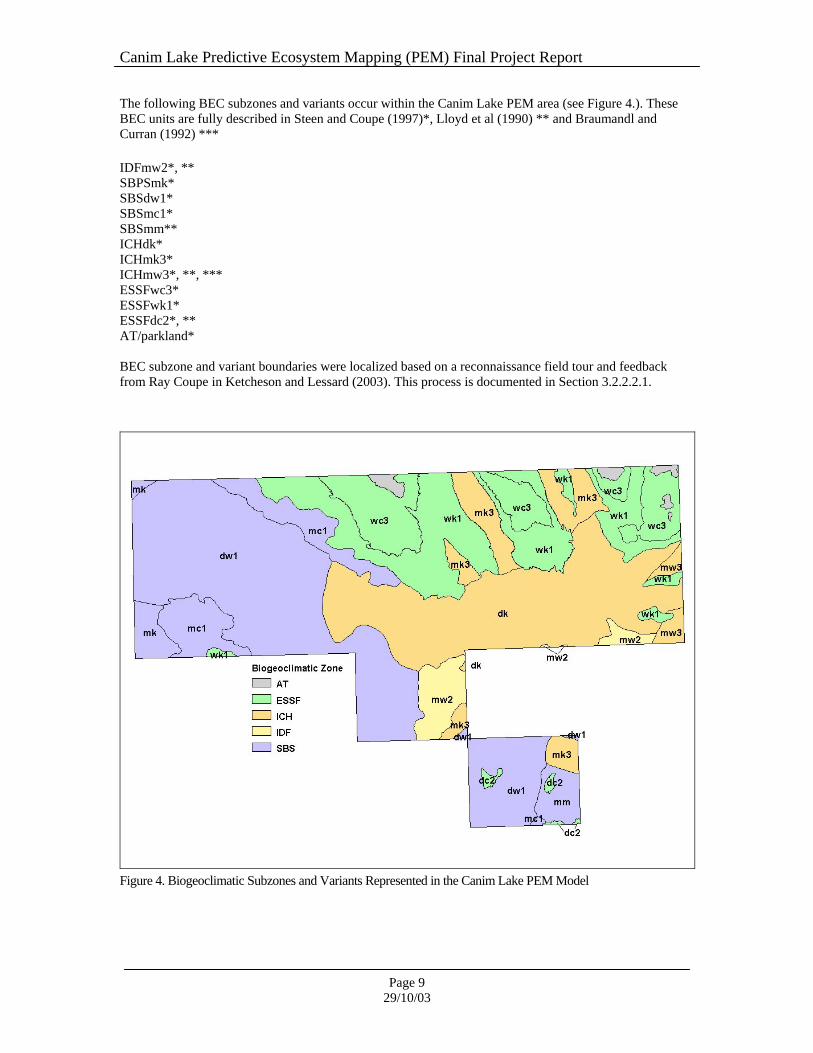
The following BEC subzones and variants occur within the Canim Lake PEM area (see Figure 4.). These BEC units are fully described in Steen and Coupe (1997)*, Lloyd et al (1990) ** and Braumandl and Curran (1992) *** IDFmw2*, ** SBPSmk* SBSdw1* SBSmc1* SBSmm** ICHdk* ICHmk3* ICHmw3*, **, *** ESSFwc3* ESSFwk1* ESSFdc2*, ** AT/parkland* BEC subzone and variant boundaries were localized based on a reconnaissance field tour and feedback from Ray Coupe in Ketcheson and Lessard (2003). This process is documented in Section 3.2.2.2.1.
Figure 4. Biogeoclimatic Subzones and Variants Represented in the Canim Lake PEM Model

Canim Lake Predictive Ecosystem Mapping (PEM) Final Project Report
Page 10 29/10/03
1.4 Geology and Geomorphology A modified terrain mapping style has been adopted for this PEM project in an attempt to minimize the time and cost while retaining the required input and reliability of a terrain layer within the PEM model. This approach has led to a terrain layer that is simpler than a traditional bioterrain mapping layer, but more specific to the needs of PEM modeling. While photos require less work to complete, they are designed to be more specific to the needs of the particular PEM model. The terrain layer produced is to be used in conjunction with the LMES model applied to a TRIM based digital elevation model (DEM) producing a direct-to-site-series map.
1.4.1 Physiographic Outline The study area lies predominately within the Fraser Plateau physiographic region. The north west corner beyond Canim Lake lies within the Quesnel Highlands physiographic region. Both of these sub regions are encompassed within the Interior Plateau (Holland, 1976). Relief across the study area is typically low to moderate (200 m to 600 m vertical relief from valley bottoms to ridge tops), with the highest elevations occurring in the north. Deception Mountain just north of the study area boundary rises to over 2300 m elevation while typical valley bottom elevations throughout the study area range from approximately 800 m to 1000 m elevation.
1.4.2 Geology Bedrock geology within the study area ranged from Quaternary (post glacial) basalt flows to Jurassic sedimentary rocks to granitics of Triassic or Jurassic origin (GSC Map 1278A, 1971). Observations in the field were consistent with the GSC geology map cited.
1.4.3 Glacial History The last glaciation is believed to have ended approximately 10,000 years ago (Holland, 1976). During the peak of the glaciation the entire land surface of the Interior Plateau would have been overlain with hundreds of meters of ice. In the region of the study area, glaciation is responsible for the deposition of the vast majority of surficial material deposits.
1.4.4 Surficial Materials Overview A wide variety of surficial materials were encountered in the study area resulting from the ultimate glaciation. A thick blanket of basal till overlies the majority of the landscape. This basal till texture is typically silt loam, loam, or sandy loam with 15 to 35 percent coarse fragments by volume. Some areas of basal till with a loamy sand or clay loam matrix texture exist, but the predominant basal till is medium textured and greater than 100 cm thick overlying bedrock. As a result of the down wasting style of deglaciation and the large amount of melt-water that would have been present at such a time in history, many glaciofluvial, ablation till, and glaciolacustrine deposits also are present in the landscape. The glaciofluvial deposits typically consist of sorted gravelly sands. A variable capping of loamy sands to sandy loams is occasionally observed on these otherwise coarse textured, thick materials. Ablation till deposits are observed to overlie basal till deposits in some locations. By nature, ablation tills are typically coarse though they can be highly variable as they are deposited in an environment with significant melt-water dissipation. The glaciolacustrine deposits encountered in the study area are typically fine textured

Canim Lake Predictive Ecosystem Mapping (PEM) Final Project Report
Page 11 29/10/03
and located in low elevation, depressional areas. Classic glaciolacustrine landforms were seldom observed in association with the known deposits within the study area. Other surficial material deposits encountered in the study area include active fluvial plains in valley bottoms (typically coarse textured), colluvial deposits on steep valley side slopes (medium to coarse textured), organic accumulations in wet depressions, and exposed bedrock in highlands and ridge tops. 2.0 Project Objectives The overall objective is:
• To produce a predictive ecosystem map (PEM) for a timber supply area (TSA) of operational interest to Weldwood of Canada Limited in the vicinity of Canim Lake using the Direct-to-Site-Series methods developed for the Cariboo PEM pilot.
The specific sub-objectives are:
• To confirm the ability of the Digital Direct-to-Site-Series methods to produce accurate, cost-effective PEM maps for significant areas on an operational basis. • To verify costs, time requirements and expected levels of map accuracy for the Digital Direct-to-Site-Series procedures when applied on an operational basis.
• To produce a cost-effective predictive ecosystem map (PEM) for Weldwood of Canada Ltd’s TSA’s in the vicinity of Canim Lake (12, 1:20,000 map sheets) that will meet or exceed the provincial minimum required level of accuracy of 65%.

Canim Lake Predictive Ecosystem Mapping (PEM) Final Project Report
Page 12 29/10/03
3.0 Methods
3.1 The PEM Model The Canim Lake PEM was completed using modeling procedures that are referred to in this document as the Landmapper Environmental Solutions Digital Direct-to-Site-Series (LMES DSS) approach. Direct-to-Site-Series is a phrase used to describe a process in which the desired ecological classification (Site Series) is interpreted or computed directly without recourse to a complex set of digital procedures for overlay and analysis of multiple digital themes. The phrase was first coined by Dr. David Moon (Moon, 2002) in his role as project monitor for the PEM pilot project carried out in the Cariboo Forest Region of BC in 2001-2002. He identified a need to examine an alternative to conventional PEM with its multiple digital overlays and complex rule bases. He suggested an alternative approach in which an experienced ecologist and photo interpreter would review high resolution stereo images using SoftCopy viewing technology and would directly interpret the most likely Site Series while viewing this 3D imagery. The idea behind this suggestion was that an experienced ecologist and photo interpreter, who was knowledgeable about the ecological classes defined for a given area, was likely to be able to manually delineate and classify Site Series more rapidly, correctly and consistently than a comparable digital PEM process. Results for the Cariboo PEM pilot appeared to vindicate this view. The manual Direct-to-Site-Series approach proved to be one of the most accurate methods (63%) and was among the most cost-effective ($0.64 per hectare). It proved to be both more accurate and lower in cost than all of the traditional PEM alternatives (Moon, 2002). In his role as project monitor, Dr. Moon also suggested that a digital equivalent to the manual Direct-to-Site-Series approach be developed and evaluated. The digital Direct-to-Site-Series approach was designed to test the theory that, instead of using landform classes as one intermediate layer in a traditional PEM process, Site Series could be predicted directly, using essentially only TRIM II DEM data and derivatives computed from the DEM data. Again, results from the Cariboo PEM pilot appeared to vindicate this view. The digital Direct-to-Site-Series (DSS) approach developed by LMES for the Cariboo PEM pilot achieved an average accuracy of 66% at a cost of $0.47 per hectare using available TRIM II DEM data. The digital Direct-to-Site-Series approach developed by LMES is, in most respects, similar to pre-existing LMES procedures used to classify landform facets. The main difference is that instead of classifying landform facets, the output from the classification procedures is a prediction of the most likely Site Series class. The original LMES toolkit was modified slightly to permit application of different rules and classification of different entities (Site Series) for different portions of a region (e.g. sub-divisions of BGC Sub-zones). An additional modification of the LMES toolkit permitted consideration of input layers not derived exclusively from processing of a raster DEM (e.g. maps of material texture and depth). Other than these minor changes, the procedures followed to predict Site Series directly are virtually identical to those used to predict the original LMES landform facets.
3.1.1 An Overview of PEM Processing Steps The LMES DSS procedures for automatically computing Site Series for the Canim Lake PEM are summarized below. • The names, definitions and differentiating attributes of all ecological units required to adequately map the study area were reviewed and identified. • A DEM with a 10 m grid spacing was obtained that encompassed the entire study area for the Canim Lake PEM project.

Canim Lake Predictive Ecosystem Mapping (PEM) Final Project Report
Page 13 29/10/03
• The full area DEM was processed to identify and correct any obvious errors or artifacts and to ensure that hydrological consistency was enforced (e.g. mapped streams “burned in” and all lakes ensured to be flat). • The 10m DEM for the full area was sub-divided into 12 tiles, with each tile encompassing an entire 1:20,000 map sheet plus a buffer around the map sheet. • The LMES program FlowMapR was applied to compute full flow topology for both upslope and down-slope flow for each of the 12 1:20,000 map tiles.
• Flow topology is a critical input required to compute relative landform position for use in subsequent classification programs.
• The LMES program FormMapR was applied to the DEM for each of the 12 map tiles to compute a full suite of terrain derivatives for each of the 12 map tiles. • All other spatial data layers deemed necessary for recognition of the defined ecological entities were obtained (e.g. maps of material texture, depth and exceptions, remotely sensed imagery, localized BGC Sub-zones). • The additional, non-DEM spatial data layers were collated and reformatted as DBF files for each of the 12 map tiles for use in the LMES programs. • Fuzzy knowledge rule bases were constructed to classify all ecological mapping entities identified as required for each of the 12 BGC Sub-zones that occurred within the Canim Lake PEM project area (see next section for details). • The initial LMES fuzzy knowledge rule bases were applied iteratively within a number of selected “training areas” and the results were used to revise and improve the fuzzy knowledge rules until such time as they produced acceptable results for all ecological classes in each BGC Sub-zone. • The LMES FacetMapR program was applied using the final “approved” Site Series rule bases to classify each grid cell in each map tile into its most likely Site Series classification for each of the 12 1:20,000 map sheet tiles. • The Site Series classifications for all 12 map sheet tiles were merged to form a single seamless, composite mosaic with no obvious edge effects. • A procedure was applied to the single seamless grid cell mosaic that removed small isolated classified areas and replaced them with the dominant classification of the surrounding grid cells in order to produce larger contiguous zones with a single consistent classification. • The resulting slightly smoothed grid map of ecological classifications was generalized to produce fewer, larger, more compact and simpler classified entities that were then described in terms of their proportions of ecological classes. • The raster ecological classification grid maps were converted into vector files in Arc/Info format and checked to ensure that they were topologically correct and that all polygons were labeled with a correct and appropriate ecological classification.

Canim Lake Predictive Ecosystem Mapping (PEM) Final Project Report
Page 14 29/10/03
3.1.2. A Summary of the Procedures used to Develop and Refine Direct-to-Site-Series (DSS) fuzzy knowledge rule bases The following steps were followed in developing and applying custom rule bases to directly predict the ecological units (Site Series) for the Canim Lake PEM project area. • The PEM mapping entities (site series or ecosystem units) identified as requiring prediction for each BGC Sub-zone were listed and their defining attributes were identified using the appropriate published Field Guides and ecological keys with additional input from the Regional Research Ecologist. • The Regional Research Ecologist reviewed and approved the numbers and types of ecological units (Site Series or other ecosystem units) to be defined for the Canim Lake PEM project area and the key attributes needed to classify these units. • Initial LMES DSS fuzzy knowledge rule bases were developed for each of the 12 BEC Sub-zones in the Canim Lake PEM project area. These rule bases built upon existing LMES Site Series rule bases previously developed for the Cariboo PEM pilot project. • A limited number of smaller test data sets were extracted for selected “training areas” within the Canim Lake PEM project area (9 training areas). • These “training area” data sets were used to apply and evaluate the initial, working LMES DSS Site Series fuzzy knowledge rule bases and their resulting PEM classification outputs. • The results of applying the initial LMES DSS fuzzy knowledge rule bases in each of the training areas were reviewed visually and obvious errors or departures from how the Site Series concepts were depicted by the Landform Profiles and in the ecological keys in the published Field Guides were identified. • The working LMES DSS fuzzy knowledge rule bases were revised iteratively to achieve maximum possible agreement between the conceptual descriptions of the agreed to list of ecological units in the published Field Guides and keys, and the spatial pattern displayed on the maps produced by applying the rules to the “training area” test data sets. • The initial set of LMES DSS fuzzy rules and the PEM maps produced by applying these rules to the selected “training areas” were reviewed in detail by the Regional Research Ecologist during a week long “modeling workshop” held in Williams Lake, Feb 3-7, 2003. • The Regional Research Ecologist systematically produced a complete list of comments identifying concerns with the classifications achieved in the “training areas” and providing suggestions for improvements and changes to the rules. • LMES implemented successive revisions of the fuzzy knowledge rule bases for each BGC Sub-zone and applied the revised rule bases to the training areas until the Regional Research Ecologist indicated that the resulting PEM maps appeared to provide an acceptable approximation of the concepts portrayed for each defined ecological class in the published Landform Profiles and ecological keys. • The “nearly final” LMES DSS fuzzy knowledge rule bases were applied to data sets for all 12 map tiles defined for the Canim Lake PEM project area to compute the full set of defined ecological classes. • PEM maps produced by applying the LMES DSS procedures to data for all 12 map tiles in the Canim Lake PEM project area using the current “nearly final” fuzzy knowledge rule bases were produced and sent to the regional ecologist as digital images and data sets for his review and comment by March 30, 2003.

Canim Lake Predictive Ecosystem Mapping (PEM) Final Project Report
Page 15 29/10/03
• The Regional Research Ecologist provided one last set of comments containing suggestions for changes to the LMES DSS fuzzy knowledge rule bases by April 30, 2003. • LMES undertook one final effort to revise and improve the LMES DSS fuzzy knowledge rule bases to respond to the suggestions made by the regional ecologist in his comments of April, 2003. • The results of applying the “final” LMES DSS fuzzy knowledge rule bases to all 12 1:20,000 map sheet tiles included in the Canim Lake PEM project were sent to the regional ecologist as digital image files for his final review and comment. • The regional ecologist indicated that he accepted that LMES had achieved as close a match as was likely feasible between the pattern of spatial distribution of ecological entities predicted by the LMES DSS procedures and rules and the pattern that best matched the ecologist’s expectations and local experience. • The regional ecologist indicated that the PEM maps produced for the 12 map tiles included in the Canim Lake PEM project appeared to be acceptable and approved the maps and the LMES DSS fuzzy knowledge rule bases used to produce them. • The PEM model of the 12 1:20,000 map tiles produced, using these final approved and accepted LMES DSS fuzzy rules, were used to construct a single seamless mosaic for the entire Canim Lake PEM project area that was used as the basis of the final PEM map submitted to the client and to the provincial digital data base. The final version of the Canim Lake PEM model was rendered and documented such that it would satisfy the requirements of the PEM Provincial Data Warehouse and met the Resources Inventory Committee (2000) for PEM digital data capture and submitted to the Digital Data Warehouse as per the appropriate specifications.
3.2 Data assembly, assessment and preparation The PEM Standards require comprehensive documentation of all methods of data assembly, assessment or preparation that depart in any way from defined standards (see Figure 1). All input data used for the Canim Lake PEM was assembled by JMJ Holdings Inc. of Nelson BC. As part of this data preparation process, JMJ prepared an assessment of input data quality for all non-standard input data layers (e.g. the “non-RIC” map of material depth and texture). JMJ documented all custom or non-standard procedures used to prepare or pre-process any of the input data layers. This applies particularly to procedures used to process the original TRIM II DEM data into a raster DEM considered suitable for use in the LMES DSS procedures. The required input data quality assessment reports prepared by JMJ are presented in Appendix A of this report. These reports identify the source and quality of the input data, knowledge bases and structural stage models used in the Canim Lake PEM and are named respectively TIDQ_CAN.rtf, TKNB_CAN.rtf and TSTS_CAN.rtf. They are required by the RIC (2000) digital data capture standards.
3.2.1 Identification and assessment of appropriate input data sets The Canim Lake PEM benefited from experience acquired in the previously completed Cariboo PEM Pilot Project (Moon, 2002, MacMillan, 2002). This initial pilot project provided an opportunity to apply various approaches to producing PEM-like maps that used a variety of different combinations of input data layers. The results from the PEM pilot identified which input data layers were most useful in producing PEM maps of acceptable predictive accuracy and which input data layers were less useful for incorporation into a PEM.
Canim Lake Predictive Ecosystem Mapping (PEM) Final Project Report
Page 16 29/10/03
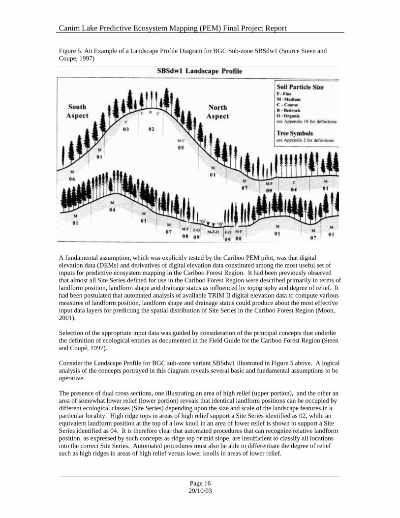
Figure 5. An Example of a Landscape Profile Diagram for BGC Sub-zone SBSdw1 (Source Steen and Coupe, 1997)
A fundamental assumption, which was explicitly tested by the Cariboo PEM pilot, was that digital elevation data (DEMs) and derivatives of digital elevation data constituted among the most useful set of inputs for predictive ecosystem mapping in the Cariboo Forest Region. It had been previously observed that almost all Site Series defined for use in the Cariboo Forest Region were described primarily in terms of landform position, landform shape and drainage status as influenced by topography and degree of relief. It had been postulated that automated analysis of available TRIM II digital elevation data to compute various measures of landform position, landform shape and drainage status could produce about the most effective input data layers for predicting the spatial distribution of Site Series in the Cariboo Forest Region (Moon, 2001). Selection of the appropriate input data was guided by consideration of the principal concepts that underlie the definition of ecological entities as documented in the Field Guide for the Cariboo Forest Region (Steen and Coupé, 1997). Consider the Landscape Profile for BGC sub-zone variant SBSdw1 illustrated in Figure 5 above. A logical analysis of the concepts portrayed in this diagram reveals several basic and fundamental assumptions to be operative. The presence of dual cross sections, one illustrating an area of high relief (upper portion), and the other an area of somewhat lower relief (lower portion) reveals that identical landform positions can be occupied by different ecological classes (Site Series) depending upon the size and scale of the landscape features in a particular locality. High ridge tops in areas of high relief support a Site Series identified as 02, while an equivalent landform position at the top of a low knoll in an area of lower relief is shown to support a Site Series identified as 04. It is therefore clear that automated procedures that can recognize relative landform position, as expressed by such concepts as ridge top or mid slope, are insufficient to classify all locations into the correct Site Series. Automated procedures must also be able to differentiate the degree of relief such as high ridges in areas of high relief versus lower knolls in areas of lower relief.

Canim Lake Predictive Ecosystem Mapping (PEM) Final Project Report
Page 17 29/10/03
Most Landscape Profiles illustrated situations in which different Site Series were shown to occur in identical landform positions, with the differences being attributed to differences in the texture (and sometimes the depth) of the underlying surficial geologic material. Figure 5 demonstrates that sites with identical landform positions, in areas of relatively low relief and low slopes, are shown to be capable of being classified as either Site Series 01, if they are underlain by medium textured materials, or Site Series 04, if they are underlain by coarse textured materials. Similar situations were observed with the Landform Profiles and classification keys for most BGC sub-zones and variants in the Cariboo Forest Region. It was therefore concluded that it was absolutely necessary to be able to identify any large areas in which the texture or depth of the underlying surficial material differed significantly from the normal, or modal, condition which was generally associated with deep, medium textured, well drained soils. It is clear from an examination of the SBSdw1 Landscape Profile (Figure 5) that, within areas characterized by a particular size and scale of topographic features (degree of relief), and by a particular texture and depth of parent material (at the level of medium, coarse or fine), the spatial arrangement of almost all identified Site Series was defined in terms of relative landform position, relative moisture status, landform orientation (aspect) and relative slope gradient. Relative landform position is generally described in terms such as crest or ridge top, mid slope, toe slope, depression or flat. Relative landform position can be approximated by several terrain derivatives that can be computed rapidly and easily from a digital elevation model (DEM). Moisture status is defined in the ecological field guides using terms such as xeric, mesic and hygric which are essentially classes that break up a continuum of moisture conditions that range from very wet to very dry. Relative moisture status generally increases in progressing from upper landform positions (crests) to the lowest positions in the landscape (valleys, draws and depressions) and can be approximated quite well using a terrain derivative referred to as wetness index that is also easily computed from a DEM. The Landscape Profile shown in Figure 5 illustrates clearly that different Site Series occur in equivalent landform positions depending upon aspect or a combination of aspect and slope gradient (e.g. steep SW or NE slopes). Aspect is easily computed from a DEM. Finally, both in the Landscape Profile diagrams and in the ecological classification keys, it was clear that certain Site Series were restricted to occurring on certain ranges of slope gradient that is also easily computed from a DEM. During the previously completed Cariboo PEM Pilot project, efforts had been made to try to model the spatial distribution of both material texture and depth and local relief using derivatives of digital elevation data. These efforts did not prove to be capable of producing results that were superior to those obtained by means of a rapid manual visual classification of material texture and depth and local landform relief. It was therefore decided that the Canim Lake PEM project would obtain information on material texture and depth and on degree of local relief from manually interpreted and manually digitized maps created at the lowest possible cost and with the lowest possible expenditure of time and effort. For the Canim Lake PEM, therefore, the spatial distribution of major differences in the texture and depth of surficial materials was obtained through reference to maps of material depth and texture prepared by JMJ Holdings Inc. on contract to Cariboo Site Productivity Adjustment Working Group (see Section 3.2.2.2.2). These maps also delineated a number of other classes of features that were judged to lend themselves well to rapid and accurate visual assessment. These other features that were mapped manually through visual interpretation of imagery and other existing maps included open water in lakes and ponds, non-forested wetlands, non-forested uplands (meadows and pastures), excluded areas (provincial parks and urban or build up areas), and bare rock. It was strongly believed that it was preferable to directly interpret and map features that could be easily and unambiguously observed and interpreted from available imagery and other sources rather than to try to extract such features through automated modeling procedures. The underlying assumption was that it was better to map directly what is easily mapped and to only model those spatial entities that were difficult, time consuming and costly to try to interpret and map manually (e.g. the forested Site Series). For the Canim Lake PEM, the spatial distribution of major differences in amount of relief was obtained through reference to a map that depicted zones of high versus low relief that was prepared internally by LMES. This map was digitized manually but identification of the high versus low relief zones was

Canim Lake Predictive Ecosystem Mapping (PEM) Final Project Report
Page 18 29/10/03
informed and guided by visual interpretation of several terrain derivatives computed from the DEM. The DEM derivatives that were found to be useful in guiding the delineation of areas of high versus low relief were wetness index, log of the diffuse upslope area and absolute distance from a cell to a channel (Z2st) as discussed below.
3.2.2 Preparation of appropriate input data sets
3.2.2.1 DEM preparation DEM data was received as individual 1:20,000 mapsheets in ARC GENERATE format. Generate files are just ASCII files that are formatted for reading by ARC/Info or ArcView. Each TDEM.GEN file was merged into one large ASCII text file. This was converted to a shapefile using ArcView’s Import Data Source utility, preserving their elevation values. The resulting shapefile was converted to an Arc/Info point coverage, and then re-projected into UTM 10 NAD 83. The TWTR layer (hydrographic features) contains point data describing various features. Some of these points are ‘sinks’ (known topological depressions). These points (FCODE HB27550000) were selected and converted to an ARC/Info point coverage, preserving their elevation values. The resulting coverage was re-projected into UTM 10 NAD83. Streams and lakes were also taken from the TWTR layer. All streams (definite, indefinite, and intermittent) were used to make the DEM. Lakes (definite, indefinite, and intermittent) were polygonized and used to ‘flatten’ water bodies. These coverages were then re-projected into UTM 10 NAD83. TRIM neatlines were concatenated into a single coverage, and re-projected to UTM 10 NAD83. The ARC/Info TOPOGRID command was used to create the DEM. TOPOGRID <out_grid> <cell_size> Arguments <out_grid> - the grid to be created. <cell_size> - the cell size, in map units, of the output grid. A cell size of 10 meters was chosen at the request of the client. A wide array of subcommands are available when using this command, but I will only list the ones used. BOUNDARY keyword and parameter for input of a polygon coverage representing the outer boundary of the interpolated grid. The concatenated TRIM neatline coverage was used as the boundary. DATATYPE the primary type of input data. Valid arguments for this are SPOT or CONTOUR. Since points are being used instead of contours, SPOT was chosen. ENFORCE turns the drainage enforcement routine on or off. The default is on. This option was left ON to enforce hydrological consistency. LAKE a polygon coverage of lakes.

Canim Lake Predictive Ecosystem Mapping (PEM) Final Project Report
Page 19 29/10/03
The polygonized lake coverage was used here to insure flat lakes. POINT keyword and parameters for input of a point coverage representing surface
elevations. The DEM point coverage was specified here along with the attribute containing elevation values. SINK keyword and parameters for input of a point coverage representing known
topographic depressions. The point coverage containing known topological depressions was specified here, along the attribute containing elevation values. STREAM keyword and parameters for input of a line coverage representing streams. The streams coverage created from the TWTR layer was specified here. TOLERANCES a set of tolerances used to adjust the calculations of the interpolation and
drainage enforcement process. These tolerances are used to adjust the smoothing of input data and the removing of sinks in the drainage enforcement process. Tolerances are listed below. {tol1} - this tolerance reflects the accuracy and density of the elevation points. Data points which block drainage by no more than this tolerance are removed. This should be set to half of the contour interval when using contour data. The default is 2.5. If input data are sparse, this parameter may be set to a higher value to produce a more generalized output grid. As there was an abundance of input data, this was set to 1. {horizontal_std_err} - this parameter represents the amount of error inherent in the process of converting point, line, and polygon elevation data into a regularly spaced grid. It is scaled by the program depending on the local slope at each data point and the grid cell size. The default value is 1.0. Larger values will cause more data smoothing, resulting in a more generalized output grid. Smaller values will cause less data smoothing, resulting in a sharper output grid (which is more likely to contain spurious sinks and peaks). Any non-negative value is permitted. Recommended values are between 0.5 and 2.0. The default value of 1 was used. {vertical_std_err} - this parameter represents the amount of random (non-systematic} error in the z-values of the input data. In most elevation data sets, it should be set to the default value of 0. If the data contains significant random vertical errors, with uniform variance, set this parameter to the standard deviation of the errors. The default value of 0 was used. The resulting DEM was then smoothed twice. The first smoothing operation was a low pass filter using a focal mean with a 3x3 kernel. The second smoothing operation was a focal mean with a 5x5 kernel. The resulting DEM was saved, and lake elevations were re-applied to the DEM to ensure that the smoothing did not displace the flat water bodies. A hillshade was then prepared to check for obvious errors.

Canim Lake Predictive Ecosystem Mapping (PEM) Final Project Report
Page 20 29/10/03
3.2.2.2 Preparation of manually interpreted and mapped data sets The LMES DSS procedures use several input variables that are mostly mapped manually and are not computed by processing DEM data. These include localized BEC mapping and generalized materials mapping. Most of these input variables were extracted from the map of material depth, texture and other exceptions that was prepared as a custom input to the procedures. The map of material depth, texture and exceptions was intended to provide a reduced subset of information relative to more traditional Bioterrain maps. This reduced sub-set of information was less expensive and time consuming to collect and was also believed to be more capable of providing the specific input data needed to support PEM predictions, as implemented by the LMES approach.
3.2.2.2.1 Localized BEC Mapping As a consequence of field sampling and liaison between ecologist Keyes Lessard of JMJ Holdings Inc. and Ray Coupe, Regional Ecologist, Cariboo Region elevation rules were created for guidelines whilst re-mapping the BEC lines within the Canim Lake PEM area. These elevation rules were derived through field observation of BEC variant, existing mapping and certain tree species distribution rules (see Table 2). Elevation rules were applied to existing BEC superimposed on TRIM contours and thematic forest cover mapping. BEC lines were adjusted by hand where appropriate and digitized based on the rules outlined in Table 2. Draft maps were reviewed by Ray Coupe and adjustments made based on his comments. Final maps were presented in digital format as seamless coverage in ARC export (e.00 format) and as a plot file in .rtl format. The mapping was accepted by Ray Coupe as interim localized BEC lines pending intensive field verification in 2003. Coupe and Steen (2003) are in the process of further revising those BEC lines, however, these lines were not available within the timeframe allocated for the Canim PEM pilot project. Final mapping meets (PEM Data Committee, 2000) digital data standards and is presented in UTM zone 10 NAD 83 based on TRIM II data with BEC lines feature coded.

Canim Lake Predictive Ecosystem Mapping (PEM) Final Project Report
Page 21 29/10/03
Table 2. Elevation Rules and Comments Used in BEC Localization of the Canim Lake PEM Area.
BEC variant Elevation Rules Comments
IDFMW2 Up to 1100 metres See Kamloops Field guide for description(Lloyd et al 1990) Variant includes Birch.
SBPSmk 1000 – 1350 metres
ICHdk 900 – 1250 metres North of Canim Lake Not a lot of Birch Use Cedar for boundary between SBSdw1 near Lang Lake No western hemlock
ICHmk3 780 – 1250 metres South of Canim Lake A firm elevational line
ICHmw3 400 – 1400 metres Includes western hemlock A flexible elevational line used western hemlock as guideline.
ESSFwc3 1500 – 1800 metres Alpine above and ESSFwk1 below
ESSFwk1 1250 – 1500 metres Below ESSFwc3
ESSFdc2 1400 – 1900 Small area south of Canim Lake, leave existing BEC lines intact
AT/Parkland > 1800 metres

Canim Lake Predictive Ecosystem Mapping (PEM) Final Project Report
Page 22 29/10/03
3.2.2.2.2 Generalized Materials Mapping A modified terrain mapping style has been adopted for this PEM project in an attempt to minimize the time and cost while retaining the required input and reliability of a terrain layer within the PEM model. This approach has led to a terrain layer that is simpler than a traditional bioterrain mapping layer, but more specific to the needs of PEM modeling. While photos require less work to complete, they are designed to be more specific to the needs of the particular PEM model. The terrain layer produced is used in conjunction with the LMES DSS model .
3.2.2.2.2.1 Mapping Criteria The terrain mapping criteria used is outlined in Table 3. Soil texture and surficial material thickness are the two variables to be used from the terrain mapping in the future PEM modeling. The boundaries between textural and thickness categories are based on what has been used in the site series classifications for the area. Both the texture and thickness attributes have been assigned a numeric value. This value roughly represents the surficial material thickness (in cm) overlying bedrock for the thickness category, and can be interpreted as the likelihood of the material being coarse textured for the textural category. Soil drainage, a key variable in the PEM modeling process, has not been mapped in the terrain layer. Drainage is being determined using a hydrological flow model (Quinn et al., 1991) based on a TRIM DEM. The terrain layer will be used to enhance the drainage model through material thickness and texture inputs. Only the surficial material texture and thickness attributes will be used from the terrain layer; surficial material type and surface expression have been mapped for the purpose of aiding the mapper in making interpretations only. Symbols have been generalized and do not reflect the detail one would expect in a typical bioterrain map.
Table 3. Canim Lake PEM Terrain Mapping Criteria
____________________________________________________________________________ Material Texture (T) •organic •fine (Si, SiL with <20% coarse fragment volume and C, SiC, SiCL, CL, SC, HC with <35% coarse fragment volume) •medium (SL, L, SCL with <70% coarse fragment volume, Si and SiL with > 20% coarse fragment volume, and C, SiC, SiCL, CL, SC, and HC with >35% coarse fragment volume) •coarse (S and LS, also SL, L, SCL with >70% coarse fragment volume) Material Thickness (D)
•EXPOSED BEDROCK
•thin material (<50cm thick) •thick material (>50cm thick) Surficial Material and Surface Expression Terrain symbology is consistent with the British Columbia terrain mapping standard (Howes and Kenk, 1997) which is found in Appendix III, with the following exceptions:

Canim Lake Predictive Ecosystem Mapping (PEM) Final Project Report
Page 23 29/10/03
Table 3. Canim Lake PEM Terrain Mapping Criteria continued….. NT wetland that does not support tree growth; could include organic plains, organic veneers, or mineral soil (surficial material texture and thickness will not be applied to the NT category). HM high elevation meadows that do not support tree growth; typically wet soils (surficial material texture and thickness will not be applied to the HM category). NP non-productive brush; typically alder patches on slopes relating to seepage zones (surficial material texture and thickness will not be applied to the NP category). _____________________________________________________________________________
3.2.2.2.2.2 Generalized Bioterrain Mapping Methodology The terrain mapping was conducted for the entire study area through air photo interpretation on black and white air photos (1999) at a scale of approximately 1:40,000. The TRIM maps within the study area boundary and the air photos used are outlined in Table 1 in the Introduction. A pre-field meeting was held in the form of a telephone conference call on Oct. 11th, 2002. Tedd Robertson and Jen Shypitka of JMJ Holdings Inc, Al Hicks and Sandra Neill of Weldwood, Ray Coupe of the MoF, Nona Phillips of MSRM, Dave Moon of CDT Core Decision Tech Inc., and Bob MacMillan of LandMapper Environmental Solutions Inc. participated in the meeting. Topics discussed related to mapping criteria, field sampling methodology, and project timing. Mapping did not follow the standard British Columbia procedures for terrain classification (Howes and Kenk, 1997). Mapping criteria was decided upon based on requirements specified for the LMES DSS model. Field work was completed after the photos had been reviewed and target site locations had been determined based on air photo interpretation. Areas of potentially coarse textured materials and thin materials were the primary ground truthing targets. Tedd Robertson, GIT, and Jen Shypitka, P.Geo, completed the mapping in October and November, 2002. An internal quality assurance review of the mapping was performed by Jen Shypitka, P.Geo. at the same time. Much discussion on the nature of the study area and air photo interpretation of the observed surficial material deposits took place between the two mappers in order to maintain consistency within the project area. Existing soil, surficial geology, and bedrock geology maps were reviewed prior to and throughout the mapping process. Existing terrain stability mapping (TSM) overlapping with three TRIM sheets within the study area was reviewed during the mapping process, and a selection of field sites from the TSM were used to aid in making interpretations. Each site from the TSM used was reviewed for the purpose of assessing its likely spatial and data reliability. Existing TEM mapping for the general area was acquired; however, did not overlap the current study area. Personal communication with colleagues familiar with the general study area also provided insight into the nature and variability of the terrain that could be expected.
3.2.2.2.2.3 Surficial Materials Field Work Methodology Field work was planned and completed using the 1:40,000 scale air photos, 1:30,000 scale orthophotos, and 1:30,000 TRIM based topographic maps. Field work was carried out by two field crews, each with a geomorphologist and an ecologist, from Oct. 16th through the 19th 2002. The crews consisted of two geomorphologists, Tedd Robertson, GIT, and Jen Shypitka, P.Geo, and two ecologists Keyes Lessard and Cory Bird. Both terrain and site series data were collected. Ray Coupe, Regional Ecologist, BC Forest

Canim Lake Predictive Ecosystem Mapping (PEM) Final Project Report
Page 24 29/10/03
Service (Williams Lake) accompanied each field crew for a full day (two days in total) and Sandra Neill of Weldwood accompanied one field crew for a day. Targeted areas included potentially coarse textured glaciofluvial and ablation till complexes as well as potentially thin soils over bedrock. While field sites were distributed throughout the entire study area, emphasis was placed on areas with easy access due to the constraint of time. Rough notes were taken on the maps identifying terrain boundary locations as well as other relevant information (material thickness, material texture, etc). Specific sites were plotted on the photos where more in-depth information was collected. These formal field sites consistently included the following interpretations and data collection, and were recorded on the standardized provincial ground inspection forms (GIF): •UTM coordinates (Garmin GPS II Plus derived); •elevation; •terrain label; •material thickness; •material texture; •coarse fragment content; •bedrock type (if applicable); •soil drainage; •BEC variant; and •site series. Other relevant information was also recorded varying from site to site. This typically included slope position, slope gradients, indicator plants, structural stage, and spatial variability of terrain and/or site series. Plot forms and project report (Robertson et al. 2002) were submitted to Al Hicks, Weldwood 100 Mile Division as part of a separate contract.
3.2.2.2.2.4 Comments on Mapping Methodology and Criteria The terrain mapping that has been performed is in many ways significantly simpler than a traditional bioterrain map. Because of this it is also significantly faster to complete and provides only the basic terrain attributes required for this particular PEM modeling. It should be recognized; however, that while being simpler this mapping does provide textural information for every polygon. This is something that a traditional bioterrain map will not necessarily provide. In many cases this textural information can be quite accurate where consistent materials exist with only minor spatial variability in texture (ie. thick blankets of medium textured basal till). Given the characteristics of the subdued topography and nature of the down-wasting style of deglaciation that has occurred in the region of the study area, many low lying areas consist of highly variable surficial material complexes. Materials that were deposited in direct contact or near proximity with down-wasting ice often can form a continuum between ablation till and glaciofluvial materials, depending on the degree of glacial water influence on the material deposition. Ablation till deposits alone, by nature, can contain a high degree of textural variability within a very small area. These areas are difficult to assign a single textural class, and generalizations must be made. In such cases the believed dominant textural class has been assigned to the entire polygon. Field checking provides a valuable insight into the general terrain of a study area as well as detailed information on specific sites within the area. The amount of field checking that was completed (see Table 10, Section 4.1) was able to increase the reliability of the mapping significantly through the confirmation of thickness and texture in difficult to interpret terrain.

Canim Lake Predictive Ecosystem Mapping (PEM) Final Project Report
Page 25 29/10/03
3.2.2.2.2.5 Generalized Terrain Mapping Spatial Data Capture Generalized terrain mapping was completed on 1:40,000 black and white air photos (see Table 1). Polygons were rendered into digital, spatially correct data using TRIM control high level photos using the methodology described below.
3.2.2.2.2.5.1 High Level (1:65000) Aerial Photographs
3.2.2.2.2.5.1.1 Same scale pin prick control transfer Control point transfer from controlled diapositives to same scale paper print was accomplished using the pin prick method on a light table. The resultant controlled paper print was utilized to create orthophotos of the 1:65,000 air photos. The control transfer involved pin pricking the high level paper print with control points derived from the archived high level diapositives. The light table and a Sokkisha zoom stereoscope was used and is necessary in order to accurately locate the small (50 micron) drill hole in the emulsion of the diapositive for each control point. In the case of a strip of 3 photos A, B, and C, photo B would have points transferred from the centerline of photos A, B and C. The point positioning would be: 3 points at the west edge of the frame, 3 points at the east edge of the frame, and one point each at the top center and bottom center. Each respective point was identified stereoscopically (4-6 X zoom) with a table top stereoscope, pin-pricked and then identified with an indelible ink circle centered on the pin prick The associated photogrammetric point number was also annotated next to the point. A control file containing the respective NAD 83 coordinates for each of the TRIM aerial triangulated control points was provided by the Ministry of Sustainable Resource Management, Base Mapping and Geomatic Services Branch. Control transfer was completed by Andrew Neale of Digital Mapping, Victoria B.C. to standards for control and data capture using mon-restitution (Standard for Ecosystem Mapping (TEM) – Digital Data Capture in British Columbia, Section 3.3.2).
3.2.2.2.2.5.1.2 Scan aerial photographs The annotated air photos were scanned at a resolution of 600 dpi on an Epson 836XL scanner using Adobe Photoshop Limited (V5.0) – Silverfast software. This scanner was used as it is able to scan up to a resolution of 6000 dpi, it is capable of scanning the air photo prints, and the radiometric quality of the scan was not a factor. Scanning at this resolution allows for an orthophoto spatial resolution of 1.5 m this exceeds plotting scales of 1:20000 which require a maximum pixel size of 2.5 m as specified by the British Columbia Specifications and Guidelines for Geomatics Digital Orthophoto, Volume 7, Section 7.7. The scanned files were saved as a TIFF file, <photo_number>.tif.
3.2.2.2.2.5.1.3 Create orthophotos In PCI OrthoEngine (V8.1) a new project was opened: set the projection parameters as follows: Projection: UTM Zone 11 (48 N to 56 N) Earth model: NAD83, Canada Output Pixel Spacing: 1.5 m

Canim Lake Predictive Ecosystem Mapping (PEM) Final Project Report
Page 26 29/10/03
Next the standard aerial camera calibration information was provided. The calibration information is obtained from Calibration of Aerial Survey Camera to the Specification for Aerial Survey Photography documents obtained from the Province of British Columbia web pages (http://home.gdbc.bc.ca/catalog/air_photo_ftp.htm) . These provide focal length and fiducial point positions. The approximate photo scale was also entered. Next an air photo was entered into the project and opened. The fiducial points for each photo were then collected. To collect a point, zoom in on the image to at least 1:1 resolution. Place the cursor precisely on the fiducial mark. Click on the "Set" button for the corresponding mark. Errors are generally in the range of 0.010 to 0.040mm. The error (in mm) is found by transforming the fiducial mark positions on the photo in pixels and lines, into photo mm. The error indicates how far off the computed value is from the specified camera calibration fiducials. An acceptable error value should ordinarily fall within the resolution of the scanning device used to digitize the original image. Once each photo has been entered into the project the next step is to collect ground control points (GCP) for each photo. Using the TRIM model control file (obtained from the Ministry of Sustainable Resource Management, Base Mapping and Geomatic Services Branch) the x (easting), y (northing), and z (elevation) coordinates for each annotated point (9 points per photo) on the air photo are entered. When all the GCPs have been collected the Model Calculation option is used. This calculation (bundle adjustment) is a method of performing the exterior orientation calculations, while considering all of the project photos. Computed this way, the image exterior orientations are a global reflection of the project data. Each point has a known ground location and elevation. For GCPs, this is provided. The ground position and elevation are fed into the exterior orientation, and a pixel and line position in the orthorectified file is computed. For each point, a corresponding position in the file was collected. The difference between the computed value and this given value is the point's residual (Root Mean Square error, RMS). The RMS error is calculated using the following equation (PCI,V8.0, Help): RMS error = [ ] sqrt [ (sum i = 1 to n (X(i) - X(org, i))^2 + (Y(i) - Y(org, i))^2) ] [ ------------------------------------------------------------ ] [ (n - 1) ] where: X(i) = computed x value of the ith point Y(i) = computed y value of the ith point X(i, org) = original x value of the ith point Y(i, org) = original y value of the ith point Editing of the GCPs is undertaken next to reduce the Root Mean Square (RMS) error to an acceptable level. Editing involves observing the Residual X and Residual Y errors provided in the Residual Error Report (see example provided below) and moving the GCP point appropriately in the x and/or y direction. Updated model calculations are done instantaneously as the GCPs are edited. For the 1:65000 air photos a RMS of less than 3.00 is obtained. When an acceptable RMS error is obtained, orthophotos can then be produced using cubic convolution as the image rectification algorithm (British Columbia Specifications and Guidelines for Geomatics Digital Orthophoto, Volume 7, Section 7.2). A DEM, generated from TRIM tdem files for each 1:20,000 BCGS map sheet, was used.

Canim Lake Predictive Ecosystem Mapping (PEM) Final Project Report
Page 27 29/10/03
3.2.2.2.2.5.2 Generalized Bioterrain Line work / 1:40,000 Aerial Photographs
3.2.2.2.2.5.2.1 Scan aerial photographs and bioterrain line work The 1:40,000 aerial photos are scanned in at a resolution of 400dpi, allowing for an output resolution of 1.0 m. The bioterrain line work, drawn on a separate piece of mylar, has been registered to the air photo fiducial points and are indicated with dots. The mylar is scanned in separately as Line Art at a resolution of 100 dpi. This is an acceptable resolution due to the coarseness of the line work. The scanned files are saved as a TIFF file, <photo_number>.tif.
3.2.2.2.2.5.2.2 Prepare the digital air photos In PCI XPACE all of the air photos are imported in to a .pix file, which is the native file format for PCI, using the FIMPORT command. Next the air photos that have been photoyped have another channel added using PCIMOD which will contain the line work.
3.2.2.2.2.5.2.3 Register the line work In PCI GCPWorks the line work file is registered to the air photo using the fiducial points on both the air photo and the mylar as the reference points.
3.2.2.2.2.5.2.4 Create orthophotos The same procedure as described in Section 3.2.2.2.2.5.1.3 is undertaken to set up the OrthoEngine project. In addition to GCPs, tie points are also collected. Tie points are conjugate points common to two or more overlapping air photos and are an additional source of control in the bundle adjustment calculation. The GCPS for the 1:40,000 air photos are collected from the orthorectified 1:65000 air photos. This is extremely useful as it allows for GCPs to be collected evenly over the entire image, rather than just where there is TRIM data such as roads and water features. The same procedure is followed in producing the orthophotos.
3.2.2.2.2.5.2.5 Bioterrain line work extraction In order to edit the bioterrain line work it must be extracted from the *.pix file. This is done in PCI Image Works using the File-Utility-Tools-Subset option and selecting the second channel that contains the line work. The line work is save as a TIFF file.

Canim Lake Predictive Ecosystem Mapping (PEM) Final Project Report
Page 28 29/10/03
3.2.2.2.2.5.3 Bioterrain line work
3.2.2.2.2.5.3.1 Line work preparation The *.tif file is opened in ArcView (V.3.1) and is converted to a grid using the Theme - Convert to Grid function. Next the grid is reclassified so that the line work is 1 and everything else is a 0, or no data. Using the Analysis - Reclassify function values from 0-10 are specified as 1 and 11-254 are specified as No Data. This reclassified grid is then saved as another grid using the Theme - Convert to Grid function. In Arc/Info (V8.0) the grid is converted using the GRIDLINE which converts a grid representing raster line features to a line coverage. Arc:gridline <in_grid> <out_cover {positive / data} {thin / nothin} {nofilter / filter} {round/ sharp} {item} {thickness} {dangle} {weed} Arc:gridline <in_grid> <out_cover> positive thin filter round # 28 0 2 Next CLEAN is used to generate a coverage with arc topology and to eliminate dangling arcs. Arc: clean <in_cover> {out_cover} {dangle_length}{fuzzy_tolerance}{poly/ line} Arc: clean <in_cover>{out_cover} 28 .01 line
3.2.2.2.2.5.3.2 Edit the line work In ArcEdit, open the coverage and edit the line work to eliminate additional dangles and gaps in the line work. Some editing is necessary as thin sinuous lines, such as river channels are often pinched in spots during the transformation from a grid to an arc coverage. Once the line work is edited, line work from air photos in an area (i.e. 1:20,000 map sheet) are appended together using the APPEND command. Arc: append <out_cover> {feature_class} Arc: append <out_cover> line Next it is necessary to edit the line work again to make the arcs contiguous between air photos.
3.2.2.2.2.5.3.3 Labeling When the bioterrain line work for an area is completed it is opened in Arcview. A new point theme is created. Labels are added and numbered to match with the polygon numbers previously assigned.
3.2.2.2.2.5.3.4 Create polygons Once the line work and labeling is completed the point shapefile is converted to a label coverage and is inserted into the line work coverage using the PUT command in ArcEdit. Next the coverage is cleaned using CLEAN and then built into a polygon coverage using BUILD.

Canim Lake Predictive Ecosystem Mapping (PEM) Final Project Report
Page 29 29/10/03
3.2.2.2.2.6 Database Creation and Format Polygons were hand labeled by the terrain typer and the information inked onto acetates registered to the air photo and polygon outlines. The data was captured into an EXCEL database using a format modified from standard PEM/TEM bioterrain databases (Ecological Data Committee, 2000). We used a slightly modified version of the standard bioterrain database with some columns removed and new columns added. Depth, texture, water, swamp, non productive brush, and high elevation meadow were added to the database. When a polygon was labeled NT (swamp), NP (non productive brush), HM (high elevation meadow) or N (water) a 1 was put in the corresponding column. Columns for drainage data were removed and fewer columns for geomorphological class and subclass were used. We entered field verification plot numbers into the comments column. Appendix C contains terrain symbology used within the database. Definitions of standard column headings can be found in Appendix C.
3.2.2.2.2.6.1 Database Internal Quality Assessment During the digital database capture, polygon line work was checked and edits made to the lines when necessary. To check the polygon contents, check maps were generated with the polygon labels. Using these maps each line of the database is compared to the air photos and corrections are made to the database where necessary. The database can be found in Appendix C.
3.2.2.2.3 Manipulation of Manually Interpreted and Mapped Data Sets For most Site Series definitions, it is sufficient to know whether the underlying parent material is significantly coarser or finer than normal or if it is shallower than 50 cm to bedrock. All other texture or depth distinctions provide more detail than required by current Site Series definitions and providing such detail simply increases costs and increases the likelihood of being incorrect. Table 4 lists the key inputs provided by the maps of material depth and texture and explains how they were interpreted or used in the PEM process.

Canim Lake Predictive Ecosystem Mapping (PEM) Final Project Report
Page 30 29/10/03
Table 4. Manually mapped input variables used in the LMES approach to PEM classification
No. Name Description Concept approximated 1 Texture Material texture value as mapped
on the map of material depth, texture and exceptions
Some Site Series were defined as occurring on materials that were coarser or finer than normal. We used a number of 50 for medium, 70 for coarse and 20 for fine texture.
2 Depth Value for depth to bedrock as mapped on the map of material depth, texture and exceptions
Some Site Series (usually 02) are defined as occurring only where soil depth is < 50 cm. This field is mainly used to identify areas where the soil is mapped as shallow.
3 Seepage A binary class (0/1) used to identify areas that are wetter than expected.
Used mainly to identify coarse textured areas that are wetter than expected rather then drier than normal.
4 Water A binary class (0/1) used to identify areas of open water
Areas of water were obtained from the TRIM II digital data and the Forest Cover maps and verified and mapped by JMJ.
5 Swamp A binary class (0/1) used to identify non-forested wetland areas
Areas of non-forested wetland were obtained from the Forest Cover digital maps and verified and mapped by JMJ.
6 Brush A binary class (0/1) used to identify non-forested areas of brush
Areas of non-forested upland brush were interpreted from available imagery, then verified and mapped by JMJ.
7 Meadow A binary class (0/1) used to identify non-forested areas of high elevation meadows
Areas of non-forested upland in high elevation meadows were interpreted from available imagery, verified and mapped.
8 Ridge A binary class (0/1) used to identify high ridges
Some Site Series were defined as occurring only on higher ridges. This class permited such ridges to be identified and mapped directly.
9 Not Mapped
Areas excluded from the PEM Mapping
Some areas were excluded from the PEM mapping for various reasons.
The JMJ map of material texture, depth and exception classes was converted to a grid map with the same dimensions and grid size (10 m) as the master DEM used to define the Canim Lake study area. Each grid cell in this master grid file was labelled with an integer ID number that corresponded to the polygon ID number on the vector ArcView coverage of the JMJ map of material texture, depth and exceptions. A separate map of grid code ID numbers was then prepared for each 1:20,000 map sheet tile for all 12 1:20,000 map sheets included in the Canim Lake PEM. The ArcView GRID map of grid code ID numbers was exported as a binary FLT file, converted from binary to ASCII and then imported into a DBF format table as illustrated below (Figure 6). The field named Gridcode in Figure 6 was used as a key field to relate information for any vector polygon mapped by JMJ to a specific grid cell in any grid map created for any of the 12 1:20,000 map sheet tiles in the Canim Lake PEM study area. A database script was written that read in the polygon attribute table for each Gridcode ID number and extracted from it the data required to fill all the fields illustrated in Figure 6.

Canim Lake Predictive Ecosystem Mapping (PEM) Final Project Report
Page 31 29/10/03
Figure 6. Illustration of the DBF format table used to hold all manually mapped input data
Data required for the fields labeled Depth, Texture, Water, Swamp, Brush, Meadow and Not_mapped were read in exactly from the map of material texture, depth and exceptions prepared by JMJ. Data in other fields in this table were added from other sources in response to unexpected needs that arose during the development and improvement of the LMES DSS rule bases. The field Elev simply contains the elevation of each grid cell. It was added to the ID#Geo DBF table when it was determined that elevation was a necessary attribute of each grid cell required to differentiate frost prone from non frost prone Site Series in one particular BGC Sub-zone. The field Seepage was added when it was determined that several polygons that had been mapped as having a coarse texture were also wetter than normal due to seepage or an elevated water table. These areas of coarse texture materials did not behave as expected for coarse textured areas. Specifically, they did not exhibit drier than normal Site Series in equivalent landform positions but instead tended to exhibit wetter than normal Site Series in equivalent landform positions. It was necessary to find some way to differentiate areas of coarser textured materials that were drier than normal from areas of coarser textured materials that were wetter then normal. An integer value of 1 in the field Seepage in the ID#Geo table is a flag that identifies to the LMES DSS modeling procedures situations when coarse textured areas are wetter than normal. Areas of coarse textured materials that were wetter than normal were identified manually by the regional ecologist. It was then a simple matter to assign an integer value of 1 to the field Seepage for any grid cell that belonged to a JMJ polygon that had been mapped as coarse but was also deemed to be wetter than normal. It was simply a matter of finding the Gridcode value that corresponded to the polygon number of an area identified as wetter than normal and inserting a value of 1 into the field Seepage for all grid cells that had this Gridcode.
The field Ridge in Figure 6 was also inserted after the initial procedures had been set up. This field was used to identify grid cells that were judged to occur on high ridges. Integer values of 1 in this field indicate that the grid cell is judged to occur on a high ridge. This field was used to help differentiate Site Series that are typically labeled as 02 and described as occurring on the driest portions of high ridges from Site Series that are typically labeled as 04 and described as occurring on the tops of lower ridges and knolls. The JMJ map of material texture, depth and exclusions was concluded to have mapped shallow materials (< 50 cm) more extensively than expected by the regional ecologist. This resulted in an initial over-estimate of the extent of dry crest type Site Series (02) relative to the expectations of the regional ecologist when 02 type
Canim Lake Predictive Ecosystem Mapping (PEM) Final Project Report
Page 32 29/10/03
units were defined as occurring at all locations where the mapped depth of soil was < 50 cm. In an attempt to rectify this over-estimation of dry ridge Site Series, the field Ridge was added to the data table and all areas previously mapped by JMJ as having a depth to bedrock of < 50 cm were judged to belong to high ridges. The rules for recognizing 02 type Site Series were adjusted to define this Site Series as occurring only on the highest and driest potions of ridges that had been classified as high ridges in the ID#Geo file. This allowed the model to constrain the estimated spatial extent of these dry ridge Site Series. The fields B3 and B5 were also added to the ID#Geo file after the initial set up and design of the model rules. These two fields contain raw digital numbers for bands 3 and 5 of the LandSat7 TM geo-registered satellite imagery for the Canim Lake PEM study area. These satellite imagery data were found to be useful for differentiating 3 non-forested ecological classes in the Atp Sub-zone. The Atp Sub-zone, by definition, cannot contain any forested Site Series. The rules and input data bases used to recognize forested Site Series were found to not apply within the Atp Sub-zone. For this sub-zone only, therefore, it was determined that applying a simple threshold value to two bands of raw satellite imagery data was useful for differentiating areas with no apparent vegetation from areas with a very thin, scattered vegetative cover from a third area with significant cover of dwarf trees and shrubs. Finally, the fields Z2Wet, L2Wet and N2Wet were inserted into the ID#Geo file for each 1:20,000 map sheet tile at the very last moment in response to a final request from the regional ecologist. These fields contain data that were computed automatically from the DEM and would normally have been expected to be located in one of the files that contain derivatives of DEM data. They were placed in the ID#Geo DBF table because the LMES programs that compute terrain derivatives are fixed and are not set up to compute the variables Z2Wet, L2Wet and N2Wet. These variables were computed by special programs that are not part of the normal LMES suite of terrain derivatives. They represent measures of vertical (Z) and horizontal (L, N) distance from every grid cell in a DEM to the first grid cell that occurs below it along a path of simulated overland flow that has been classified as either open water or non-forested wetland. These derivatives were computed in order to differentiate areas that were located around the margins of lakes and wetlands and that were raised only a few metres above the level of the lake or wetland. The regional ecologist requested that such areas be separated so that they could be described as having a higher than normal likelihood of containing a mixture of wetter than normal Site Series. The only convenient DBF table in which to store these data proved to be the ID#Geo table, so the three extra fields of data were added to this file for each of the 12 1:20,000 map sheet tiles.
3.2.2.3 Preparation of data sets computed automatically from the DEM For the Canim Lake PEM, a gridded DEM was created with horizontal dimensions of 10 by 10 m and a vertical resolution of no better than ±10 m absolute (perhaps better than ±5 m relative). A separate DEM tile was then extracted from the master DEM for the entire Canim Lake area for each of the 12 1:20,000 map sheet tiles included in the PEM project. The elevation data for each of the 12 tiles were exported from ArcView and reformatted for use in the LMES DSS programs. The LMES program FormMapR was used to compute a large number of terrain derivatives for each of the 12 map sheet tiles. Ultimately, only a few key derivatives were actually used in defining Site Series classes for the Canim Lake PEM, but the entire suite of terrain derivatives computed by the LMES programs was available for consideration as possible input data for the PEM classification procedures. All terrain derivatives actually used to define Site Series in the Canim Lake PEM are listed in Table 5, along with the ecological or geomorphic concepts they are intended to approximate. As stated previously, the LMES DSS approach seeks to identify a single input variable, or at most 2 variables, that best approximate each of the critical concepts that are used to define Site Series ecological classes in the appropriate ecological field guides. The variables listed in Table 5 were selected specifically to act as direct one-to-one analogues for a specific concept such as relative slope position or relative moisture status. We made every effort to adhere to the principal of “parsimony of parameters” which states that a model should use as few input variables as possible, but as many as are needed. Our experience confirmed the importance of this principal as we encountered problems with unstable and

Canim Lake Predictive Ecosystem Mapping (PEM) Final Project Report
Page 33 29/10/03
unpredictable classification results whenever we used too many inputs. The fewer the inputs, the easier it was to understand and tune the model.
Table 5. Terrain derivatives computed and used in the LMES approach to PEM classification
No. Name Description Concept approximated 1 LnQarea Log of diffuse upslope area as
per Quinn et al., 1991 Used to approximate the concept of relative landform position as expressed by such terms as crest, upper, mid, lower or toe. These terms are defined using fuzzy logic.
2 Qweti Wetness Index as per Quinn et al., 1991
Used to approximate concepts of relative moisture status as expressed in the field guides by such terms as xeric, mesic and hygric. These formal terms are not used so as to avoid confusing the fuzzy classes defined by LEMS with the more strictly defined formal terms.
3 Slope Slope gradient in % computed as per Eyton, 1991.
Used mainly to identify steep SW or NE slopes, gentle SW or NE slopes, or very flat areas.
4 New_Asp Slope aspect in degrees computed as per Eyton, 1991.
Used mainly to identify steep or gentle SW or NE slopes. The original value for aspect has been shifted counter clockwise by 45 degrees to facilitate applying fuzzy calculations to identify SW and NE.
5 PctZ2Str Relative landform position computed as percent vertical distance (Z) above a defined stream cell relative to a crest cell.
Used as a supplementary measure of relative landform position in cases where the LnQarea does not work adequately. Used mainly to identify lower and toe slope positions subject to seepage or frost accumulation.
6 Z2St Vertical elevation (Z) of a cell above the nearest cell that it flows to that is classed as a channel, or stream, cell
Used as a measure of absolute relief of a cell above local stream or base level. Used mainly to identify areas that may belong to high ridges or to low-lying flood plains.
7 Elev Absolute elevation (m) Used where elevation is used to define a Site Series attribute (frost hazard).

Canim Lake Predictive Ecosystem Mapping (PEM) Final Project Report
Page 34 29/10/03
Figure 7. Illustration of the terrain derivative log of upslope area for a portion of map sheet 93a006
Figure 7 illustrates the appearance of the terrain derivative that measures the log of the diffuse upslope area (Quinn et al., 1991) for a portion of map sheet 93a006. A considerable amount of trial and error went into deciding to use this variable as the principal analogue to represent relative slope position. Other variables, such as percent vertical distance from stream to divide (PctZ2St) were available and were considered. Ultimately, this variable was considered to provide the most effective measure of relative landform position for the purposes of recognition of Site Series in the Canim Lake PEM. One advantage of using diffuse upslope area as a surrogate for relative landform position is that it tends to exhibit a smooth continuous monotonic increase in value in progressing down slope from the tops of ridges to the bottoms of valleys. This variable is particularly effective for differentiating upper portions of the landscape corresponding to crests, upper slopes, and mid slopes. A disadvantage of using diffuse upslope area to represent relative slope position is that it becomes somewhat less reliable when used to identify lower to toe slopes and valleys. This is because it is not truly a measure of relative landform position but is rather a measure of absolute upslope contributing area. As slopes get longer, high values for diffuse upslope area tend to occur higher and higher upslope. Areas that would be considered to represent valley bottoms and depressions in an area of low relief and shorter slopes will almost certainly have values for diffuse upslope area that are lower than the value for diffuse upslope area computed for a mid to lower portion of a very long slope in an area of high relief. This limitation of the variable diffuse upslope area needs to be recognized and accounted for. The variable can only be used in a relative sense within areas that have similar landforms with similar slope lengths and upslope contributing areas. Different threshold values for upslope areas were used to differentiate lower to toe slope positions in different portions of each BGC Sub-zone depending upon whether the area was classified as having high relief (and long slopes) or lower relief (and shorter slopes). This adjustment allowed the variable to be used in a relative sense to approximate relative landform position, as long as it was being compared to values computed for other areas with similar slope lengths and upslope contributing areas.

Canim Lake Predictive Ecosystem Mapping (PEM) Final Project Report
Page 35 29/10/03
A second limitation of the variable diffuse upslope area is that it is highly sensitive to flow divergence and tends produce spatial patterns that reflect high flow accumulation in lateral draws and valleys, while not producing similarly high accumulation values that would permit recognition of lower and toe slope positions. Spurs running in a dominant down slope direction can have very low values for diffuse upslope area and will therefore be considered to be located near a crest, even in instances where they are actually located in a lower or toe slope position in the larger context. In several BGC Sub-zones, rules based on using log of upslope area as the sole measure of relative landform position did not perform adequately and an additional measure of relative landform position (PctZ2St) had to be included in the fuzzy classification rule definitions. The terrain derivative wetness index (Quinn et al., 1991) was used as a direct analogue to relative moisture regime as indicated by the terms xeric, mesic and hygric in the ecological classification field guides. We did not use terms such as mesic, hygric or xeric to describe classes of relative moisture regime defined as fuzzy landform attributes so as to avoid confusion with the formally defined terms. However, the intent was the same, namely to divide the continuum of the potential moisture gradient into classes that reflected conditions that were normal (mesic), drier than normal (xeric, sub-xeric, sub-mesic) and wetter than normal (sub-hygric, hygric and sub-hydric). As illustrated in Figure 8, the variable wetness index does a creditable job of identifying areas that are likely to be drier than normal (ridges and spurs) and wetter then normal (draws, hollows and valleys). Figure 8. Illustration of the terrain derivative Wetness Index for a portion of map sheet 93a006
Figure 9. Illustration of the terrain derivative new_asp for a portion of map sheet 93a006

Canim Lake Predictive Ecosystem Mapping (PEM) Final Project Report
Page 36 29/10/03
As with log of diffuse upslope area, to which wetness index is related, this derivative is more consistent as a measure of relative dryness than wetness. The tops of all ridges are all recognized to have a low wetness index. High wetness index values occur in both valleys and draws and in lower toe slope positions. The very wettest and very driest sites do appear to be well delineated by this variable. Slightly wet intermediate sites are not consistently identified in the same relative landform locations. Still, the derivative does follow a logical pattern of indicating higher relative moisture regimes as one progresses further down slope in the landscape into valleys and draws. Slope gradient was computed using the finite difference algorithm of Eyton (1991). Slope gradient is used to directly match slope criteria used to define or describe Site Series in the Field Guides. Some Site Series are defined as occurring only on steep slopes and others are defined as being restricted to gentle slopes. New-Asp is simply a re-orientation of aspect computed using the finite difference algorithm of Eyton (1991) See Figure 9. The absolute value for aspect was rotated 45° counter clockwise and stored in the field new-asp. This rotation was done to facilitate the application of fuzzy rule definitions for NE and SW aspect. By rotating the value for aspect by 45° counter clockwise, it became easier to compute likelihood of having a NE orientation using a central value of 90° and a spread of ± 45° all the way up to ±90° without having to address the issue of going counter clockwise past the value of zero due to the circular nature of the variable aspect. Similarly, the fuzzy definitions for likelihood of having a SW orientation could be centered on a value of new_asp of 270° with a spread of up to ±90° without going over a value of 360° and re-entering a zone of small values that begin with 0°. Rotation of the original value for aspect was simply a convenience implemented to make calculation of fuzzy likelihood values for likelihood of having a NE or SW orientation somewhat easier. This derivative was mainly used to help identify Site Series that were defined as having a steep SW or steep NE orientation. It was also used to identify a smaller number of Site Series that were defined as having a gentle SW or gentle NE orientation. The gray level coloring of Figure 9 illustrates this capability well, as SW facing slopes appear in lighter shades of gray and NE facing slopes appear darker.
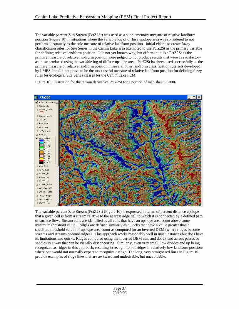
Canim Lake Predictive Ecosystem Mapping (PEM) Final Project Report
Page 37 29/10/03
The variable percent Z to Stream (PctZ2St) was used as a supplementary measure of relative landform position (Figure 10) in situations where the variable log of diffuse upslope area was considered to not perform adequately as the sole measure of relative landform position. Initial efforts to create fuzzy classification rules for Site Series in the Canim Lake area attempted to use PctZ2St as the primary variable for defining relative landform position. It is not yet known why, but efforts to utilize PctZ2St as the primary measure of relative landform position were judged to not produce results that were as satisfactory as those produced using the variable log of diffuse upslope area. PctZ2St has been used successfully as the primary measure of relative landform position in several other landform classification rule sets developed by LMES, but did not prove to be the most useful measure of relative landform position for defining fuzzy rules for ecological Site Series classes for the Canim Lake PEM.
Figure 10. Illustration for the terrain derivative PctZ2St for a portion of map sheet 93a006
The variable percent Z to Stream (PctZ2St) (Figure 10) is expressed in terms of percent distance upslope that a given cell is from a stream relative to the nearest ridge cell to which it is connected by a defined path of surface flow. Stream cells are identified as all cells that have an upslope area count above some minimum threshold value. Ridges are defined similarly as all cells that have a value greater than a specified threshold value for upslope area count as computed for an inverted DEM (where ridges become streams and streams become ridges). This approach works reasonably well in most instances but does have its limitations and quirks. Ridges computed using the inverted DEM can, and do, extend across passes or saddles in a way that can be visually disconcerting. Similarly, even very small, low divides end up being recognized as ridges in this approach, resulting in recognition of ridges in relatively low landform positions where one would not normally expect to recognize a ridge. The long, very straight red lines in Figure 10 provide examples of ridge lines that are awkward and undesirable, but unavoidable.

Canim Lake Predictive Ecosystem Mapping (PEM) Final Project Report
Page 38 29/10/03
The variable PctZ2St was used to prevent certain Site Series (e.g. mesic 01) from occurring in some lower to toe landform positions close to or adjacent to stream channels. It was used to try to force slightly wetter Site Series to occur in some of these lower to toe slope landform positions, when such landform positions were not well recognized using the primary variable for relative landform position (log of diffuse upslope area).
Figure 11. Illustration of the terrain derivative PctZ2wet for a portion of map sheet 93a006
The variable Z2wet (Figure 11) represents a slight modification to the concept inherent in the variable Z2St and was computed by making a slight modification to the LMES program used to compute Z2St. Instead of flowing down from each grid cell until encountering a cell that is classified as a stream channel cell (as in Z2St, see Figure 13) the algorithm was modified to flow down until it encountered a cell that was classified as belonging to a body of open water or a non-forested wetland. The “target cells” used to identify calls that belonged to a lake or wetland were extracted without change from the map of material texture, depth and exceptions produced by JMJ Holdings for the project. This map identified the location and extent of all lakes and wetlands. These locations had been extracted from existing TRIM II and Forest Inventory maps and subjected to additional visual checking and verification by JMJ interpreters. The variable Z2Wet can therefore be considered to provide a measure of the vertical change in elevation from any cell to the nearest wetland or lake cell to which it is connected by a path of overland surface flow. The variable Z2Wet was only computed in the late stages of the Canim Lake PEM project. It was computed in response to a direct request from the regional ecologist to attempt to find some way of ensuring that low-lying areas around the margins of lakes and wetlands were not classified into mesic or drier Site Series, but were capable of being separated and described as consisting of some combination or mostly wetter than normal Site Series. In the context of this use, the only significant values of Z2Wet are those in the lower range (< 3-5 m) that identify cells judged to be “close to” a wetland or lake in the vertical dimension.
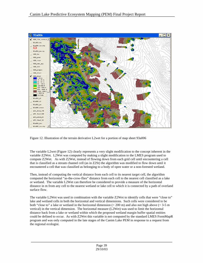
Canim Lake Predictive Ecosystem Mapping (PEM) Final Project Report
Page 39 29/10/03
Figure 12. Illustration of the terrain derivative L2wet for a portion of map sheet 93a006
The variable L2wet (Figure 12) clearly represents a very slight modification to the concept inherent in the variable Z2Wet. L2Wet was computed by making a slight modification to the LMES program used to compute Z2Wet. As with Z2Wet, instead of flowing down from each grid cell until encountering a cell that is classified as a stream channel cell (as in Z2St) the algorithm was modified to flow down until it encountered a cell that was classified as belonging to a body of open water or a non-forested wetland. Then, instead of computing the vertical distance from each cell to its nearest target cell, the algorithm computed the horizontal “as-the-crow-flies” distance from each cell to the nearest cell classified as a lake or wetland. The variable L2Wet can therefore be considered to provide a measure of the horizontal distance in m from any cell to the nearest wetland or lake cell to which it is connected by a path of overland surface flow. The variable L2Wet was used in combination with the variable Z2Wet to identify cells that were “close to” lake and wetland cells in both the horizontal and vertical dimensions. Such cells were considered to be both “close to” a lake or wetland in the horizontal dimension (< 200 m) and also not high above (< 3-5 m vertical) in the vertical dimension. The horizontal measure (L2Wet) was used to limit the horizontal distance back from a lake or wetland within which the proposed wetland margin buffer spatial entities could be defined to occur. As with Z2Wet this variable is not computed by the standard LMES FormMapR program and was only computed in the late stages of the Canim Lake PEM in response to a request from the regional ecologist.

Canim Lake Predictive Ecosystem Mapping (PEM) Final Project Report
Page 40 29/10/03
Figure 13. Illustration of the terrain derivative Z2st for a portion of map sheet 93a006
The variable Z to Stream (Z2St) (Figure 13) is a custom variable computed by the LMES program FormMapR. It is obviously one half of the calculation used to compute the relative landform position variable PctZ2St, the second half being Z2Cr. The variable Z2St measures the absolute difference in elevation from every cell in a DEM to the first cell below it that is classified as a stream channel cell and to which the cell is connected by a path of simulated surface flow. Z2St provides a measure of absolute relief, expressed as vertical distance above a cell that is defined as a stream channel cell. The variable Z2St was used sparingly in developing fuzzy classification rules for the Canim Lake PEM. Where it was used, its purpose was mainly to permit differentiation of upper slopes and ridge tops that were relatively “high up” in the landscape (e.g. had a large value for Z2St) from cells that were similarly classed as being ridges or upper slopes but that were not “high up” in the landscape (e.g. were close to a stream channel in the vertical dimension). This measure of absolute relief can be used, for example, to help differentiate Site Series that occur on the driest portions of high ridges (typically labeled as 02) from Site Series that occur on somewhat lower and more gentle ridges and knolls (typically labeled as 04).

Canim Lake Predictive Ecosystem Mapping (PEM) Final Project Report
Page 41 29/10/03
3.3 PEM Knowledge Base Creation The LMES DSS approach to predicting ecological classes (Site Series) is aimed at identifying, capturing, encoding and applying the ecological knowledge and logic encapsulated in Field Guides, keys, and local expert ecological experience in a formal, systematic and reproducible fashion. This kind of knowledge is referred to as “heuristic knowledge” and can be captured and applied by creating and applying “fuzzy knowledge” rules. Fuzzy knowledge rules are based on capturing heuristic knowledge or beliefs in a formalized, quantitative fashion. Because they aim to capture expert beliefs about conceptual classes, they can be constructed without using actual site data collected from field surveys. The approach can certainly make use of actual site data to guide in the creation and revision of fuzzy knowledge rules, should such data be available, but it does not absolutely require the availability of hard field data. Due to the constraints against collection and use of actual field data imposed as one of the conditions of the Cariboo PEM Pilot, the use of real field data to identify Site Series and to establish their defining characteristics was not part of the process used to define the PEM knowledge bases for the Canim Lake PEM. The LMES DSS approach sought to identify the key attributes used to define each Site Series concept, as outlined in the appropriate ecological Field Guide and to find single digital inputs (or less frequently combinations of digital inputs) that had a clear one-to-one relationship with these key attributes and could be used to approximate them. The Cariboo PEM Pilot Project had demonstrated that most of the key concepts used to define Site Series in the Cariboo Forest Region could be approximated using terrain derivatives extracted automatically from digital elevation data. Those attributes that could not be readily approximated using terrain derivatives were found to mostly pertain to soil texture, soil depth and readily visible exceptions such as water, non-forested wetlands, rock or non-forested uplands. The PEM Pilot demonstrated that these additional inputs could be readily obtained with sufficient accuracy by conducting a rapid and inexpensive air photo interpretation and preparing a single map of material depth, texture and exceptions that provided all additional necessary non-DEM input data.
3.3.1 The Two Main Components of a LMES DSS Knowledge Base The LMES DSS procedures use a two step approach to capturing and applying ecological knowledge that requires creation of two separate, but inter-dependant rule bases. In the first step, rules are defined that convert raw input data in numerical format (both classed and continuous) into continuous integer values that range from 0 to 100 that define “fuzzy attributes”. Fuzzy attributes express the relative likelihood (on a scale of 0-100) that a given value of a given input variable matches a specific landform concept, such as being located in a mid-slope landform position, or having a steep slope. The integer numbers between 0 and 100 provide a quantitative way of capturing and expressing semantic concepts, such as slope position. Semantic concepts are simply word-like phrases or statements that convey an idea or meaning, such as the relative slope position of a location. In the LMES DSS procedures, fuzzy attributes are defined in a DBF attribute rule file that is always assigned a name beginning with “arule”, to which is appended a number that identifies the BGC sub-zone, or sub-division of a sub-zone within which the rule applies. In a second step, the previously computed fuzzy attributes are used to define and calculate “fuzzy classes” of ecological entities. A set of word-like phrases or statements is used to specify the defining characteristics of each potential ecological class (Site Series or non-forested ecological entity) in terms of a weighted combination of fuzzy attributes. A linked set of statements phrased in terms of weighted attributes is prepared and stored for each unique occurrence or characteristic set of circumstances under which a given ecological entity is believed to occur. Previously, it was noted that a given Site Series could occupy several different landform positions simultaneously. No Site Series that occurs under several sets of different conditions can possibly be correctly recognized by a single definition. Therefore, the LMES DSS fuzzy classification rule tables contain a separate group of classification rules for each unique

Canim Lake Predictive Ecosystem Mapping (PEM) Final Project Report
Page 42 29/10/03
occurrence or situation in which a particular Site Series has been described as occurring. Rules for defining “fuzzy classes” of Site Series are stored in a second DBF rule table that is always assigned a name beginning in “crule”, to which is appended a number that identifies the BGC sub-zone, or sub-division of a sub-zone in which the rule file applies.
3.3.1.1 Fuzzy attributes and fuzzy attribute rule tables Fuzzy attributes express the degree to which a given value of a given input variable approximates a semantic concept such as wetness or relative landform position that is used to define a Site Series class. A semantic concept is simply a word such as “crest” or “dry” that is used to describe a condition believed to be definitive for a given ecological class (Site Series) of interest. Consider the example illustrated in Figure 14. This shows how words or phrases that describe concepts relating to relative landform position and relative moisture regime are defined and how they are related to landform attributes used to characterize particular Site Series classes. In Figure 14, the Site Series labeled as 02 can be seen to occupy a “crest” landform position, while 03 occupies a crest to upper (Crest2Up) landform position and 05 occupies a crest to mid slope (Crest2Mid) landform position. Each of these concepts pertaining to relative landform position has been assigned a quantitative definition in terms of an allowable upper limit, lower limit or central value and an allowable range for the input terrain derivative log of diffuse upslope area (LNQAREA). In a similar fashion, semantic concepts such as dry (Dry_wi), very dry to wet (Vdry2wet) and dry to slightly dry (Dry2SlDry) are defined in terms of ranges of the input derivative wetness index. Grid maps of each of the variables used to capture and express a semantic concept were reviewed visually. The spatial distribution of different ranges of values of these variables was observed to identify upper and lower limits that corresponded to semantic concepts such as crest or mid-slope that were used to characterize any Site Series of interest. Every effort was made to select threshold values for these input variables that would result in the placement of boundaries between defined Site Series in approximately the same relative locations as were depicted on the Landform Profile diagrams. The LMES DSS program FacetMapR uses simple equations to convert raw continuous or classed input variables into “fuzzy attribute” values that range from 0 to 100. These integer numbers express the likelihood that a particular value of a given input variable matches or meets the central concept for a fuzzy semantic construct such as being in a “crest” position or being “dry”. The more closely an input variable matches the defined central concept, the higher the integer value computed for the fuzzy likelihood that the input value represents that fuzzy concept. A value of 100 expresses complete agreement with the fuzzy concept while a value of 0 expresses complete disagreement. The LMES procedures permit any number of “fuzzy attributes” to be defined based on any number of available input variables. A guiding principal, however, is that it is best to use as few input variables as possible to define as few fuzzy attribute concepts as possible. In all cases, the standard approach is to define the minimum number of fuzzy attributes that are absolutely necessary to express all the concepts embodied in the definitions of all Site Series listed for any given BGC sub-zone. New “fuzzy attributes” based on new input variables are only defined if the initial set of minimum “fuzzy attributes” is found to be unable to effectively classify all required Site Series classes.

Canim Lake Predictive Ecosystem Mapping (PEM) Final Project Report
Page 43 29/10/03
Figure 14. Illustration of how "fuzzy attributes" quantify semantic concepts in an “arule” file
In modeling, this is known as the “principal of parsimony”. Any model should attempt to produce reliable outputs using as few input variables and as few operations as possible. Models that contain large numbers of input variables that are subjected to a large number of operations rapidly become very difficult to interpret and to control. If the LMES rule bases appear incredibly simple, this is by design. The underlying philosophy is always to try to achieve a reasonable classification result using the fewest possible input variables to define the fewest possible number of “fuzzy attributes”.
3.3.1.2 Fuzzy classes and fuzzy class rule tables The second step in the LMES DSS classification procedures involves defining and computing “fuzzy classes” expressed as a linear average of a number of “fuzzy attributes”. Any type and number of “fuzzy classes” can be defined in terms of any number of combinations of “fuzzy attributes”. For PEM mapping in the Canim Lake area, the number of “fuzzy classes” is always equal to the number of unique “situations” or “presentations” of Site Series or non-forested ecological entities recognized for each BGC sub-zone within the area.

Canim Lake Predictive Ecosystem Mapping (PEM) Final Project Report
Page 44 29/10/03
Consider the following example of how “fuzzy classes” of ecological entities were defined in terms of a weighted linear combination of “fuzzy attributes” in a “crule” file (Figure 15). The “crule” file occupies the left hand side of the workspace illustrated in Figure 15. It consists of series of entries into 5 columns. All entries required to define a particular ecological class occur together as a contiguous group of criteria or statements. The first entity defined in the illustrated “crule” table is assigned the name S1001s in the column F_name and is assigned a code value of 1001 in the column f_code. It is meant to capture the concepts inherent in the definition of a 01 Site Series that occurs on gentle SW slopes in zone 10 = SBSdw1. This entity is defined as occurring in an upper to mid landform position (Up2Mid) with a dry to medium moisture regime (Dry2Med_WI). It occurs on slopes less than 30 degrees on gentle SW facing aspects and on deep, medium textured materials. This is almost a verbatim transcription of the definition for Site Series 01 as it appears in the Cariboo Field Guide. Each of the “fuzzy attributes” used to define this ecological class was assigned an attribute weight in the column labeled Attrwt. The attribute weight tells the FacetMapR program what relative weight to assign to each attribute in computing an overall weighted average value for the likelihood that each cell or site matches the description for that ecological class as provided by the listed combination of fuzzy attributes. Each “fuzzy class” in a LMES DSS “crule” file is therefore defined as a linear combination of “fuzzy attributes” that are considered to be definitive of the class. The LMES programs read in the “crule” file to determine how many “fuzzy classes” to define in any given area, what “fuzzy attributes” to use to define each class and what label to give to a cell that is determined to be best represented by a given “fuzzy class”.
Figure 15. Illustration of "fuzzy classes" defined in terms of “fuzzy attributes” in a “crule” file

Canim Lake Predictive Ecosystem Mapping (PEM) Final Project Report
Page 45 29/10/03
The likelihood that a given cell belongs to a defined “fuzzy class” is computed by multiplying the value of each listed “fuzzy attribute” for that cell by a weighting factor that specifies the relative importance that a particular “fuzzy attribute” is assumed to exert in terms of the overall definition of the class. Fuzzy class membership values are thus computed as the sum of Fuzzy attribute(n)*Attribute Weight(n) for n = 1 to the total number of attributes used to define the class. The values for Attribute Weight(n) are normalised to sum to 1.0 before being applied in the above equation, so all resulting values for “fuzzy class” membership also range from 0 to 100 as was the case with the “fuzzy attribute” input values themselves. A value between 0 and 100 is computed for “fuzzy class” membership for every possible “fuzzy class” listed in the relevant “crule” file. In the implementation of the LMES DSS program used in the Canim Lake PEM, only one final class code is recorded for each grid cell. This class code represents the “fuzzy class” with the highest computed fuzzy likelihood value for that cell. Other implementations of the FacetMapR program store the value for the fuzzy likelihood of every possible class for every grid cell. However, this represents a very large overhead in terms of data storage and disk read/write time and so is not used for very large data sets such as in the Canim Lake PEM.
3.3.2 Initial LMES DSS Knowledge Base Creation The initial PEM knowledge base for the Canim Lake PEM was created by identifying the all significant “instances” or “situations” of all ecological entities defined for a particular BGC Sub-zone in the appropriate Field Guide and then identifying the key “fuzzy attributes” required to uniquely characterize and classify each of these entities. The spatial distribution of each of the raw input terrain derivatives used to define each identified “fuzzy attribute” was then reviewed visually to determine and select appropriate threshold values for identifying upper limits, lower limits, central values and ranges for each “fuzzy attribute” input variable for each ecological class to be defined. Fuzzy classification rule files (“crule” files) were then prepared that attempted to describe each “situation” of each required ecological class in terms of a weighted combination of the selected “fuzzy attributes”. An initial rule base was considered to have captured the concepts inherent in the definitions of ecological classes well enough to merit review by the regional ecologist. This was the case once the spatial arrangement and distribution of predicted classes more or less matched the relative conceptual arrangement of the same classes as depicted on the appropriate Landform Profile diagrams an in the keys to the ecological entities for each BGC Sub-zone. Initial development, application and evaluation of the rule bases and the results produced by applying them was carried out for a number of “training areas” selected as representative of each BGC Sub-zone or a limited number of BGC Sub-zones or variants.
3.3.3 Different Rules for Sub-divisions of BGC Sub-zones and Variants Initially, only one set of fuzzy logic rule bases was constructed for each unique BGC Sub-zone or variant. However, it rapidly became apparent that different portions of the same BGC Sub-zone often benefited from having different rule bases with different threshold values for the same fuzzy attributes and even different suites of fuzzy classes. Upon reflection, the need for and justification for further subdivision within BGC Sub-zones became obvious. Firstly, as mentioned previously, the BGC ecological classification system is designed to operate in a hierarchical fashion and this holds true even within BGC Sub-zones. The exact same landform positions or “situations” are often described as being occupied by different Site Series depending upon whether the underlying geologic materials are medium, coarse or fine textured. In fact, coarse textured areas were often described (by the regional ecologist) as having a completely different sequence of Site Series progressing from crest to hollow than medium textured areas with otherwise identical topography and relief. In formal classification terms, parent material tended to act as another level in the hierarchy, imposing limits upon which ecological classes could be expected to occur within coarser areas and changing the rules regarding

Canim Lake Predictive Ecosystem Mapping (PEM) Final Project Report
Page 46 29/10/03
which parts of the landscape were occupied by particular Site Series. It therefore became clear that parent material texture was acting as a Boolean constraint upon classification and that areas of coarser textured materials should be separated from areas of medium textured materials and should be classified differently using completely different sets of rules. Sub-division of BGC Sub-zones according to parent material permitted the rule bases for the two separate zones to become far simpler, smaller, more effective and more easily understood and tuned than was the case when a single set of rules needed to apply across the full range of material textures. Secondly, as also previously mentioned, differences in absolute and relative relief and, in particular, slope lengths, within a given BGC Sub-zone were observed to result in strikingly different patterns of spatial distribution for several of the key DEM derivatives used to define fuzzy landform attributes. This was particularly true for the key variables of log of diffuse upslope area and wetness index. Both of these variables are only effective as measures of relative landform position and relative moisture regime respectively within areas that have comparable relief and slope length. A given value for log of diffuse upslope area will occur at a very different position in the landscape in an area of long continuous slopes with large upslope contributing areas than it will in an area of much shorter slopes with lower upslope contributing area. Threshold values applied to these variables to infer relative landform position are therefore only effective within areas that have similar and comparable topography in terms of relief and slope lengths. It became obvious that BGC Sub-zones and variants should also be further sub-divided into zones of high relief and long slopes versus zones of lower relief and shorter slopes and that different rule sets, with different threshold values, should be developed for each of these two different classes of topography. Thirdly, the LMES DSS procedures needed to accommodate the decision to identify and explicitly map those clearly obvious features that were mapped directly easier, faster and more correctly using manual visual interpretation than by trying to infer their existence through a fuzzy modeling process. It just makes sense to directly map what is easily mapped and to not try to get overly complicated in modeling entities that do not need to be modeled. All features that were directly mapped were considered to be Boolean in nature, meaning that they either existed at a location or they did not. If they existed at a location, then no other potential ecological entity could also exist at that location and there was no point in computing fuzzy likelihood values for all other potential ecological classes within any areas that had been directly mapped. For this reason, every BGC Sub-zone was further subdivided to separate out all areas that had already been directly mapped. A single set of simple Boolean rules was constructed that was operative only within these “exception areas”. If a cell was located within an “exception area” it had to be one of the directly mapped spatial entities and could not be any ecological Site Series. All that was required for these areas was to look up which type of exception had already been mapped for that cell and to assign the cell to that class (e.g. lake or non-forested wetland). Separation of all directly mapped areas into a separate classification zone within each BGC Sub-zone also contributed to simplifying the rule bases for the remainder of the area and increased the speed of the classification process (as un-necessary calculations were avoided). As a consequence of the realizations discussed above, it was as determined that it would be beneficial to define and apply different knowledge base rule tables for up to 5 different sub-divisions of each BGC Sub-zone or variant. The 5 different types of sub-divisions that could occur in any BGC sub-zone are listed in Table 6. This approach necessitated construction of 5 sets of rules per BGC Sub-zone or variant times 12 Sub-zones for a total of 60 sets of paired “arule” and “crule” files. A naming convention was adopted in which the names of rule files always started with the root word “arule” or “crule”, followed by a four digit number that identified the integer ID number used to identify the BGC Sub-zone (in the hundreds to thousands place) and the nature or type of further sub-division in the ones and tens place as indicated in Table 6. Thus, a rule file with the name arule1002 would apply to BGC Sub-zone 10 (SBSdw1) and to areas of medium textured materials and high relief with long continuous slopes (e.g. X02 in Table 6). This decision required extra effort to create the classification zone map as the intersection of material texture, relief type and exception areas and to create and refine rule files for up to 5 different classification zones within each BGC Sub-zone.
Table 6. Description of the 5 functional sub-divisions possible within each BGC sub-zone

Canim Lake Predictive Ecosystem Mapping (PEM) Final Project Report
Page 47 29/10/03
No. Number Description of the reason for the sub-division 1 X00 Areas labelled “00” contain all polygon features mapped directly on the
input map of material depth, texture and exceptions. Rules for these areas classify readily observable and mappable features such as open water, non-forested wetlands, non-forested uplands or excluded areas. It was judged that it was far better to directly map spatial entities such as water that can be easily and consistently mapped by direct air photo interpretation that to attempt to predict such entities with a model.
2 X01 Rules for areas labelled “01” apply to “normal” terrain with low to moderate relief and medium textured soils.
3 X02 Rules for areas labelled “02” apply to terrain with high relief, long, continuous slopes and medium textured soils.
4 X11 Rules for areas labelled “11” apply to “normal” terrain with low to moderate relief but with coarse textured soils.
5 X12 Rules for areas labelled “02” apply to terrain with high relief, long, continuous slopes and coarse textured soils.
Rules were created to define “fuzzy attributes” and “fuzzy classes” for each of the 5 possible sub-divisions in each of the 12 BGC sub-zones found in the Canim Lake PEM, regardless of whether the sub-divisions occurred, or were needed, within a given BGC sub-zone. I some cases, rules do not vary between sub-divisions within a given BGC sub-zone. In other cases, the rules for “fuzzy classes” remain identical, but the rules for defining “fuzzy attributes” change in order to use different threshold values to change the definition of concepts such as toe slope position to accommodate changes in the values of the variables wetness index and upslope area that arise from the longer slopes and different topography.

Canim Lake Predictive Ecosystem Mapping (PEM) Final Project Report
Page 48 29/10/03
3.4 Initial PEM Classification An initial set of classification rules was developed for all 12 BGC Sub-zones and applied to 9 different “training areas” distributed throughout the Canim Lake PEM map area. These rules were applied and revised iteratively by LMES until such time as LMES was satisfied that a reasonable “conceptual match” had been achieved for all ecological classes defined in the Field Guides for all of the 12 BGC Sub-zones included in the Canim Lake PEM project (Figure 16).
Figure 16. Illustration of the location of 9 Canim Lake training areas relative to BGC Sub-zones Once LMES was satisfied that the initial set of classification rules produced a reasonable “conceptual match” with the ecological entities identified for each BGC Sub-zone in the appropriate Field Guide, a workshop was scheduled in which the input and advice of the Regional Research Ecologist was solicited and acted upon.
3.4.1 Qualitative PEM Model Assessment Process During the workshop (held Feb 3-7, 2003 in Williams Lake) the Regional Research Ecologist (Ray Coupé) reviewed all output maps for the selected training areas. He then identified discrepancies between the PEM output for these areas and his understanding of the expected distribution of the predicted Site Series in terms of both “conceptual match” and “geographic match”. LMES adjusted the rule bases to try to address the comments and suggestions of the Regional Research Ecologist and re-applied the revised rules. At the end of the workshop, the Regional Ecologist had reviewed the rules for all BGC Sub-zones and had offered his comments and advice, identifying obvious problems and suggesting improvements or solutions. LMES recorded these suggestions and returned to Edmonton to complete their implementation.

Canim Lake Predictive Ecosystem Mapping (PEM) Final Project Report
Page 49 29/10/03
The PEM rule bases were improved and adjusted iteratively by visually examining the map output achieved by application of a given set of rules and using the informed opinion of the Regional Research Ecologist to identify any needed changes or improvements. The Regional Research Ecologist reviewed all interim map results and identified instances where the distribution of Site Series predicted by the LMES DSS modeling procedures differed obviously and significantly from what he expected based on his local knowledge and experience. Qualitative evaluation and iterative improvement of the results of applying the LMES DSS PEM model rules was recognized to follow two major stages. In the first stage, modeling efforts were focused on producing output in which Site Series were distributed in an appropriate and more or less correct topographic order in the landscape. The intent of this stage was to produce a set of classification rules that placed each Site Series in a given BGC Sub-zone or variant into the correct topographic position. Such that it occupied approximately the expected topographic location (e.g. mid-slope, toe slope, crest) and was bracketed by the expected Site Series in topographic positions that were immediately above and below it. Rules were defined that placed all relevant Site Series in approximately their correct relative topographic position in the landscape. Then the rules were deemed to have achieved a correct “conceptual match” between the map entities produced by application of the rules and the map entity concepts as depicted on the Landscape Profile diagrams. Achieving a correct “conceptual match” meant that the rules were doing a good job of capturing the concepts inherent in the various Site Series definitions, in terms of relative location in the landscape but they might not yet be correctly capturing the absolute extent of specific Site Series or the correct absolute locations for boundaries between Site Series. The second stage of the LMES DSS modeling efforts therefore focused on achieving what was thought of a correct “geographic match”. A correct “geographic match” was considered obtained when the spatial distribution of Site Series predicted by the LMES DSS procedures more or less matched the expected geographic distribution, based on the local knowledge and experience of the Regional Research Ecologist. The regional ecologist reviewed maps produced by applying a given set of classification rules and identified instances where a particular Site Series occupied a greater or lesser extent of the area than his experience told him was likely to be the case. The ecologist also identified specific areas where, in his experience, a particular Site Series was known to occur. If the LMES DSS model predicted a different Site Series than expected for any of these specific locations, the model rules were adjusted in an attempt to predict the known and expected Site Series in these locations. Finally, the Regional Ecologist picked out any areas where the LMES DSS classification gave him cause for concern and reviewed aerial photos, forest cover maps and other available data sources to determine if the predicted classification was consistent or inconsistent with the distribution of tree species that could be identified using the available information sources. Again, the model rules were adjusted and the procedures were rerun to produce new interim maps after each adjustment. When the Regional Research Ecologist was satisfied that the PEM model rules were producing predictions of the geographic extent of all defined Site Series that were as reasonable, and reliable as could be attained, the rules for a particular BGC sub-zone variant were signed off by the regional ecologist as being “finalized” and “accepted”. A key stage in the process of “tuning” the LMES DSS classification rules occurred during a one week period from Feb 3 – Feb 7, 2003 when the principals involved in building and revising the LMES DSS classification rule bases met for a week long modeling workshop. Bob MacMillan and Ray Coupé were joined by Dave Moon, Nona Philips and Ordell Steen. They spent the entire week revising rule tables and running the revised rule tables to produce output maps for selected “training areas”. After each application of a revised set of rules the output was reviewed for a given “training area” or set of “training areas”. Discrepancies were identified where the output departed from expectations and suggestions were made for how to resolve the discrepancies. New rules were constructed and the new rules reapplied to generate new output. Most revisions simply involved making small changes to threshold values for variables used to define existing rules. Adjustment of threshold values was equivalent to “tuning” a rule set that had achieved a good “conceptual match” in order to move boundaries up or down or to expand or contract the extent of a given predicted Site Series in order to achieve an improved “geographic match”. One final change suggested by Ray Coupé was to define a new conceptual entity that was envisaged as consisting of low-lying areas at the margins of lakes and wetlands. This conceptual entity was devised in

Canim Lake Predictive Ecosystem Mapping (PEM) Final Project Report
Page 50 29/10/03
order to ensure that mesic and drier units did not extend right down slopes to the edges of wetlands and open water. It was envisaged to contain a relatively broad mixture of potential Site Series but to be mostly dominated by wetter than mesic Site Series in any given BGC sub-zone or variant. An initial “finalized” set of PEM rule bases and PEM maps was delivered to the client and to the Regional Research Ecologist for review on March 30, 2003. The Regional Research Ecologist reviewed these initial final results and provided detailed comments and feedback with specific suggestions for some final improvements and changes. These suggestions were received and collated by the end of April, 2003. A set of final “finalized” rule bases was constructed in response to the final suggestions of the Regional Research Ecologist. The final fuzzy logic rules and the PEM maps that they produced when applied to the Canim lake input data sets were sent to the Regional Research Ecologist (Ray Coupé) on July 11, 2003. They were reviewed by him and received his approval. The PEM maps produced using this final approved and accepted set of rule bases was used to construct a final seamless mosaic map for the entire study area that was cleaned, converted to an Arc/Info vector coverage and submitted to the provincial digital data base in a format that meets the specifications of the PEM Digital Data standards (PEM Data Committee, 2000). For more information regarding the files required for submission please see Section 4.4 of this report or Section 5.0 of the Standards for Predictive Ecocsystem Mapping (PEM) – Digital Data Standards. This coverage was submitted for an independent assessment of accuracy, the results of which can be found in Moon 2003.
3.5 Field Data Collection Field data was collected to confirm generalized materials mapping only. This is described in Sections 3.2.2.2.2.3 and 4.1. No field data were collected in support of the Canim Lake PEM and no previously existing field data were made available to LMES to use in iterative review and revision of the Canim Lake PEM knowledge base. The principal reason for not collecting or using field data to create or tune the Canim Lake PEM knowledge base was that the LMES DSS procedures were originally designed and developed to operate without the benefit of field data. The idea was to see whether adequate predictions of ecological classes could be achieved by focussing on capturing the concepts documented in published Field Guides and ecological keys. This was supplemented by tuning of model rules by having a local expert review the results of applying the rules to the available input data sets. Additional justification for not collecting and using field data to develop and train the LMES DSS models was provided by the experiences obtained during the Cariboo PEM Pilot project. In this pilot project, neither direct interpretation of Site Series by a locally knowledgeable ecologist, nor other PEM methods supported by minimal field inspections, proved able to produce PEM maps that were superior to the maps produced by the LMES DSS method. The conclusion reached was that collection of limited amounts of field data was not a guarantee that PEM rules and resulting PEM maps could be produced that were superior to those produced without the use of limited field data.

Canim Lake Predictive Ecosystem Mapping (PEM) Final Project Report
Page 51 29/10/03
3.6 PEM Map Entity Derivation Map entities are based on Steen and Coupe’s (1997) site series classification. However, it is recognized that the resolution of the PEM, at the mapping scale, can result in a somewhat generalized depiction of the landscape. Consequently, when the results of the map are compared to the reality of site series distribution on the ground, it becomes evident that large scale variability within PEM mapped site series needs to be recognized. This estimate of relative proportions of site series over a short distance accounts for the difference between what is observed on the ground and what the model predicts. This variability is described in terms of relative proportions of site series that may be found on the ground over a relatively small distance. These proportions are assigned to each map entity and can be found in Appendix E. The proportions were determined subjectively and vary between each LMES DSS map category. They are used to calculate percentage composition of site series within each final PEM polygon. A list of site series mapped by the Canim Lake PEM can be found in Table 7. A detailed discussion of the heterogeneity of map entities can be found in section 4.2.2.
Table 7. BEC Variants and Site Series Mapped by the Canim Lake PEM Pilot Project
ZONE SUB-ZONE
VAR SITE SERIE
S #
MAP CODE
SITE SERIES NAME
AT 00 LA Generic Open Water AT 00 WE Generic Non-forested wetland AT 00 ME Generic non-forested upland AT 00 MW Moss campion - Spiked wood-rush tundra
AT 00 AW Mountain-avens - Dwarf willow AT 00 FR Alpine Scrub Forest AT 00 ND NOT MAPPED
ESSF dc 2 01 FR Bl - Rhododendron - Grouseberry ESSF dc 2 02 JP Juniper - Pinegrass ESSF dc 2 03 LF PlSe - Falsebox - Pinegrass ESSF dc 2 04 FG Bl - Grouseberry - Cladonia ESSF dc 2 05 FB Bl - Huckleberry - Feathermoss ESSF dc 2 06 FO Bl - Gooseberry - Oak fern ESSF dc 2 07 FV Bl - Rhododendron - Valerian ESSF dc 2 08 FT Bl - Trapper's tea ESSF dc 2 09 SS Sedge - Sphagnum ESSF dc 2 00 LA Generic Open Water ESSF dc 2 00 ME Generic non-forested upland ESSF dc 2 00 ND NOT MAPPED ESSF wc 3 01 FR Bl - Rhododendron - Oak fern ESSF wc 3 02 FQ Bl - Rhododendron - Queen's cup ESSF wc 3 03 FG Bl - Globeflower - Horsetail ESSF wc 3 00 LA Generic Open Water ESSF wc 3 00 WE Generic Non-forested wetland ESSF wc 3 00 ME Generic non-forested upland ESSF wc 3 00 ND NOT MAPPED ESSF wk 1 01 FB Bl - Oak fern - Brachythecium ESSF wk 1 02 FF Bl - Huckleberry - Feathermoss ESSF wk 1 03 FO Bl - Oak fern - Knight's plume

Canim Lake Predictive Ecosystem Mapping (PEM) Final Project Report
Page 52 29/10/03
ZONE SUB-ZONE
VAR SITE SERIE
S #
MAP CODE
SITE SERIES NAME
ESSF wk 1 04 FT Bl - Twinberry - Lady fern ESSF wk 1 05 FD Bl - Devil's club - Lady fern ESSF wk 1 06 FH Bl - Horsetail - Sphagnum ESSF wk 1 07 FL Bl - Lady fern - Horsetail ESSF wk 1 00 LA Generic Open Water ESSF wk 1 00 WE Generic Non-forested wetland ESSF wk 1 00 ME Generic non-forested upland ESSF wk 1 00 ND NOT MAPPED ICH dk 01 RF CwSxw - Falsebox - Wintergreen ICH dk 02 RS CwSxw - Soopolallie ICH dk 03 FS CwSxw - Falsebox - Soopolallie ICH dk 04 FF CwSxw - Falsebox - Feathermoss ICH dk 05 RT CwSxw - Thimbleberry ICH dk 06 RR CwSxw - Raspberry - Oak fern ICH dk 07 ST Sxw - Twinberry - Oak fern ICH dk 08 SD Sxw - Devil's club - Lady fern ICH dk 09 SH Sxw - Horsetail ICH dk 00 LA Generic Open Water ICH dk 00 WE Generic Non-forested wetland ICH dk 00 ME Generic non-forested upland ICH dk 00 ND NOT MAPPED ICH mk 3 01 RF CwSxw - Falsebox - Knight's plume ICH mk 3 02 RM FdCw - Wavy-leaved moss ICH mk 3 03 RS CwSxw - Soopolallie ICH mk 3 04 SO CwSxw - Oak fern - Cat's-tail moss ICH mk 3 05 SF SxwCw - Oak fern ICH mk 3 06 RD CwHw - Devil's club - Lady fern ICH mk 3 07 RH CwSxw - Devil's club - Horsetail ICH mk 3 00 LA Generic Open Water ICH mk 3 00 WE Generic Non-forested wetland ICH mk 3 00 ME Generic non-forested upland ICH mk 3 00 ND NOT MAPPED ICH mw 3 01 HF HwCw - Falsebox - Feathermoss ICH mw 3 02 DJ Fd - Juniper - Cladina ICH mw 3 03 DP FdPl - Pinegrass - Feathermoss ICH mw 3 04 RS CwFd - Soopolallie - Twinflower ICH mw 3 05 RF CwFd - Falsebox ICH mw 3 06 HO CwHw - Oak fern ICH mw 3 07 RD CwHw - Devil's club - Lady fern ICH mw 3 08 RC CwSxw - Skunk cabbage ICH mw 3 09 SE Sedge - Sphagnum ICH mw 3 00 LA Generic Open Water ICH mw 3 00 WE Generic Non-forested wetland ICH mw 3 00 ME Generic non-forested upland ICH mw 3 06 HO CwHw - Oak fern ICH mw 3 00 ND NOT MAPPED

Canim Lake Predictive Ecosystem Mapping (PEM) Final Project Report
Page 53 29/10/03
ZONE SUB-ZONE
VAR SITE SERIE
S #
MAP CODE
SITE SERIES NAME
IDF mw 2 01 DF FdCw - Falsebox - Prince's pine IDF mw 2 02 DS Fd - Snowberry - Bluebunch wheatgrass
IDF mw 2 03 DP Fd - Pinegrass - Feathermoss IDF mw 2 04 SO CwSxw - Oak fern IDF mw 2 05 RS Dogwood - Sedge IDF mw 2 00 LA Generic Open Water IDF mw 2 00 WE Generic Non-forested wetland IDF mw 2 00 ME Generic non-forested upland IDF mw 2 00 ND NOT MAPPED SBPS mk 01 LP Pl - Pinegrass - Arnica SBPS mk 02 LC Pl - Cladonia - Haircap moss SBPS mk 03 FA Fd - Pinegrass - Aster SBPS mk 04 LF Pl - Pinegrass - Feathermoss SBPS mk 05 SM SxwFd - Step moss SBPS mk 06 ST Sxw - Twinberry SBPS mk 07 SH Sxw - Horsetail - Glow moss SBPS mk 08 BB SbSxw - Scrub birch - Sedge SBPS mk 00 LA Generic Open Water SBPS mk 00 WE Generic Non-forested wetland SBPS mk 00 ME Generic non-forested upland SBPS mk 00 ND NOT MAPPED SBS dw 1 01 SP SxwFd - Pinegrass SBS dw 1 02 DC FdPl - Cladonia SBS dw 1 03 DS Fd - Saskatoon - Pinegrass SBS dw 1 04 LP Pl - Pinegrass - Feathermoss SBS dw 1 05 SR SxwFd - Ricegrass SBS dw 1 06 ST SxwFd - Thimbleberry SBS dw 1 07 SC Sxw - Twinberry - Coltsfoot SBS dw 1 08 SO Sxw - Twinberry - Oak fern SBS dw 1 09 SH Sxw - Horsetail - Glow moss SBS dw 1 00 LA Generic Open Water SBS dw 1 00 WE Generic Non-forested wetland SBS dw 1 00 ME Generic non-forested upland SBS dw 1 00 ND NOT MAPPED SBS mc 1 01 SB Sxw - Huckleberry SBS mc 1 02 LC Pl - Cladonia - Haircap moss SBS mc 1 03 DP Fd - Pinegrass - Aster SBS mc 1 04 SL Sxw - Huckleberry - Labrador tea SBS mc 1 05 SS Sxw - Spirea - Glow moss SBS mc 1 SO Sxw - Oak fern SBS mc 1 07 SD Sxw - Devil's club - Step moss SBS mc 1 08 SH Sxw - Horsetail - Glow moss SBS mc 1 00 LA Generic Open Water SBS mc 1 00 WE Generic Non-forested wetland SBS mc 1 00 ME Generic non-forested upland SBS mc 1 00 ND NOT MAPPED SBS mm 01 SF Sxw - Falsebox - Knight's plume

Canim Lake Predictive Ecosystem Mapping (PEM) Final Project Report
Page 54 29/10/03
ZONE SUB-ZONE
VAR SITE SERIE
S #
MAP CODE
SITE SERIES NAME
SBS mm 02 LH Pl - Huckleberry - Cladonia SBS mm 03 LJ Pl - Douglas-fir - Juniper SBS mm 04 LS Pl - Soopolallie - Pinegrass SBS mm 05 SS Sxw - Soopolallie - Falsebox SBS mm 06 HF Sxw - Huckleberry - Falsebox SBS mm 07 SO Sxw - Oak fern SBS mm 08 SH Sxw - Horsetail SBS mm 09 SE Sedge - Sphagnum SBS mm 00 LA Generic Open Water SBS mm 0 WE Generic Non-forested wetland SBS mm 00 ME Generic non-forested upland SBS mm 00 ND NOT MAPPED
3.7 Structural Stage Model
The structural stage model for Canim Lake was completed using the localized BEC mapping and forest cover data. The input data quality report for the structural stage can be found in Appendix A (tSTS.can.rtf). The structural stage classification used follows the standards set for TEM (Ecosystems Working Group, 1998) There is a seven class structural stage model used. The structural stage classes can be found in Table 8 below.
Table 8. Structural Stages Modeled in the Canim PEM Project.
Structural Stage Code Description (Ecosystems Working Group 1998) 1 Sparse/bryoid 2 Herb 3 Shrub/herb 4 Pole Sapling 5 Young Forest 6 Mature Forest 7 Old Forest
A series of queries were developed for each BEC zone, utilizing non-forest and stand information from the forest cover to target various structural stages. A full set of queries can be found in Appendix D. An example query can be found in Table 9.
The queries were run, and the relevant structural stages were entered into an attribute called ‘STRUC’ in the database. An ArcView shapefile was then created, called ‘CANIM_STRUC’. This is a separate coverage from the PEM site series coverage.
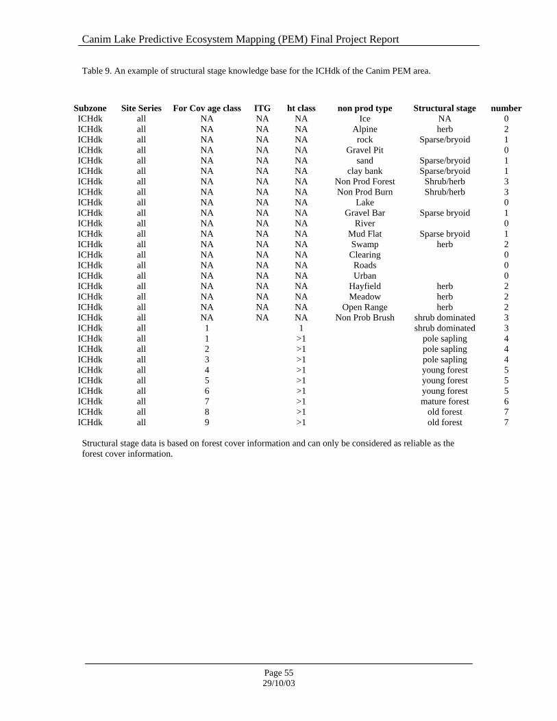
Canim Lake Predictive Ecosystem Mapping (PEM) Final Project Report
Page 55 29/10/03
Table 9. An example of structural stage knowledge base for the ICHdk of the Canim PEM area.
Subzone Site Series For Cov age class ITG ht class non prod type Structural stage number ICHdk all NA NA NA Ice NA 0 ICHdk all NA NA NA Alpine herb 2 ICHdk all NA NA NA rock Sparse/bryoid 1 ICHdk all NA NA NA Gravel Pit 0 ICHdk all NA NA NA sand Sparse/bryoid 1 ICHdk all NA NA NA clay bank Sparse/bryoid 1 ICHdk all NA NA NA Non Prod Forest Shrub/herb 3 ICHdk all NA NA NA Non Prod Burn Shrub/herb 3 ICHdk all NA NA NA Lake 0 ICHdk all NA NA NA Gravel Bar Sparse bryoid 1 ICHdk all NA NA NA River 0 ICHdk all NA NA NA Mud Flat Sparse bryoid 1 ICHdk all NA NA NA Swamp herb 2 ICHdk all NA NA NA Clearing 0 ICHdk all NA NA NA Roads 0 ICHdk all NA NA NA Urban 0 ICHdk all NA NA NA Hayfield herb 2 ICHdk all NA NA NA Meadow herb 2 ICHdk all NA NA NA Open Range herb 2 ICHdk all NA NA NA Non Prob Brush shrub dominated 3 ICHdk all 1 1 shrub dominated 3 ICHdk all 1 >1 pole sapling 4 ICHdk all 2 >1 pole sapling 4 ICHdk all 3 >1 pole sapling 4 ICHdk all 4 >1 young forest 5 ICHdk all 5 >1 young forest 5 ICHdk all 6 >1 young forest 5 ICHdk all 7 >1 mature forest 6 ICHdk all 8 >1 old forest 7 ICHdk all 9 >1 old forest 7 Structural stage data is based on forest cover information and can only be considered as reliable as the forest cover information.

Canim Lake Predictive Ecosystem Mapping (PEM) Final Project Report
Page 56 29/10/03
4.0 Results
4.1 Generalized Terrain Mapping Reliability The overall reliability or accuracy of the terrain mapping is dependant on a number of factors including: scale and quality of the air photos, skill and experience of the mapper, type and density of the vegetation, and nature of the terrain and surficial materials, and degree of field checking. The 1:40,000 scale photos are of good quality. The photos are also relatively recent (1999) and only limited development has occurred within the study area since the photos were taken. Both mappers (Tedd Robertson and Jen Shypitka) have gained some experience in the region of the study area through the terrain mapping of three TRIM sheets directly adjacent to the current study area for the Canim Lake PEM Pilot Project (Robertson et al. 2002). The combined experience of the two mappers is also considerable throughout the province including the Williams Lake area. The nature of terrain and surficial materials in the study area creates a range in reliability for different surficial material types. The complex undulating ablation till deposits overlying medium textured basal till deposits in low lying areas are considerably more difficult to map accurately in comparison with the rolling basal till blankets observed over much of the study area. It should be noted that a much greater area of terrain has been mapped with a relatively high degree of confidence compared to the difficult to interpret, highly variable, polygons of lower confidence. The survey intensity of field checking is outlined in Table 10.
Table 10. Generalized Terrain Field work sampling results
Total number of polygons 3599 Total area mapped (ha) (lakes, non-crown land, and parks excluded)
163,605
Total number of treed polygons 1940 Total number of field sites 190 Total number of coarse textured polygons 1374 Total area of coarse textured polygons (ha) 36,889 Total number of medium textured polygons 505 Total area of medium textured polygons (ha) 121,103 Total number of fine textured polygons 16 Total area of fine textured polygons (ha) 647 Total number of rock polygons 13 Total area of rock polygons 21 Total number of shallow polygons 1400 Total area of shallow polygons 18,554 Total number of thick polygons 525 Total area of thick polygons 140,202 Field checks per 1000 ha 1.2 Percent of treed polygons checked 9.8 Percent of coarse polygons checked 4.4 Field checks in coarse material per 1000 ha coarse area
2.3
Percentage of shallow polygons checked 1.1 Field checks in shallow material per 1000 ha shallow area
0.9

Canim Lake Predictive Ecosystem Mapping (PEM) Final Project Report
Page 57 29/10/03
The above table of sampling results (Table 10) refers to detailed field sites only. Field notes taken directly on the field maps and ortho photos provide additional terrain information that is not represented in the analysis of field site data compared to mapping results for reliability interpretations.
4.1.1 Terrain Mapping Reliability Assessment 190 field plots were sampled. Of these, 12 plots did not have UTM coordinates, three plots fell within private land, and one plot fell outside the study area. These plots were not used in the reliability assessment. Field plot data was compared to the final mapping and an assessment of the relationship between field plot and map was made. The relationship between field data and map results was good. Discrepancies between field data and mapping were usually the result of the field plot being located within a materials complex, and at the scale of the mapping, the map attributes did not reflect field attributes. The results of the assessment of generalized materials mapping relative to field observations is presented in Table 11. In general, 96% of the time the field data matched the generalized materials mapping.
Table 11. Reliability of Generalized Materials Mapping
Reliability For Material Depth Total Plots 174 Score 163 Percent Correct 94% Lower +/- 95% Confidence Value 156 Mid +/- 95% Confidence Value 163 Upper +/- 95% Confidence Value 169 Lower +/- 95% Confidence Interval 90% Mid +/- 95% Confidence Interval 94% Upper +/- 95% Confidence Interval 97% Reliability For Material Texture Total Plots 174 Score 167 Percent Correct 96% Lower +/- 95% Confidence Value 162 Mid +/- 95% Confidence Value 167 Upper +/- 95% Confidence Value 172 Lower +/- 95% Confidence Interval 93% Mid +/- 95% Confidence Interval 96% Upper +/- 95% Confidence Interval 99%

Canim Lake Predictive Ecosystem Mapping (PEM) Final Project Report
Page 58 29/10/03
4.2 Predicted Map Entities
4.2.1 Map Entity Allocation by PEM Model A complete list of map entities, their assumptions, applicable structural stages, site series variability within each entity and comments can be found in Appendix E. What follows in Table 13 is a list of the map entities depicted in the Canim Lake PEM model and the area of each within the study area. The PEM map entities are based on site series concepts as documented in Steen and Coupe (1997) and Lloyd et al (1990) and through description and review of site series concepts by Ray Coupe (Ecologist, Cariboo Region). It is recognized that given the resolution of the PEM, each map entity generally represents a single site series. However, on the ground a single map entity could have the likelihood of supporting one or more site series in microtopographic positions that occur at a resolution below that of the PEM. Consequently, some map entities in general describe a single site series, but could include up to two other site series. The proportions of site series within each map entity are described in Appendix E and section 4.2.2.
4.2.2 Site series/ Map entity relationships The initial mapping entities defined for the Canim Lake PEM through application of the LMES DSS procedures attempted to achieve a direct one-to-one relationship between a single Site Series concept, as depicted by the appropriate Landform Profile in the relevant Field Guide, and a classified mapping entity. In some instances, however, the available input data were judged to be incapable of supporting separation of two or more Site Series. Examples of such instances include situations where two or more Site Series could only be differentiated on the basis of slight differences in under story vegetation that were not capable of being extracted or modeled from available input data sets. In these instances, a mapping entity was defined that described a complex of two or more similar Site Series that occurred in unspecified proportions. A second example of a complex mapping entity would be one in which a unit was defined as containing a transition from one Site Series to another (e.g. some 16 units were defined as a transition from 01 through to 06 Site Series concepts). In addition, it is recognized and acknowledged that the supposedly pure mapping entities defined by application of the LMES DSS procedures are unlikely to ever consist of a single Site Series throughout their entire extent. The explanation for this is that the LMES DSS model works with input data sets and with concepts that capture and delineate Site Series entities over a particular range of scales that describes only a portion of the total variation in the spatial arrangement of Site Series in the landscape. Spatial variation in Site Series occurs over a wide range of scales in response to different influences that operate over different distances. One influence that operates over rather short distances (large scales) is micro-topography. Small changes in relief and relative landform position associated with micro-topography can, and do, result in local changes in site conditions that result in variation in Site Series classification. These small variations in micro-topography are not captured by the available TRIM II DEM data and so, are not available to help predict the correct Site Series in terms of micro-topographic position. The LMES procedures capture and portray variation in Site Series concepts that occurs over distances of perhaps 50 to 100 m that correspond to the level of spatial resolution offered by the available TRIM II DEM data. They are not able to capture variation that operates at scales of 1 to 50 m that is below the spatial resolution of any of the input data sets available for use to delineate site conditions. Consequently, any variation that occurs below the minimum spatial resolution of the input data sets (say below 20-50 m) cannot be explicitly identified and mapped by the LMES DSS procedures; it can only be inferred through sampling or estimation.

Canim Lake Predictive Ecosystem Mapping (PEM) Final Project Report
Page 59 29/10/03
The Canim Lake PEM did not have access to any field plot or transect data to provide direct field measurements to assist in determining the amount and type of fine-scale variation in Site Series classification within the notionally pure single Site Series mapping entities. This left us with no other option than to use the judgment of local ecological experts to estimate the most likely kind and amount of variation in Site Series composition within the notionally pure Site Series mapping entities. The estimates of Site Series variation provided here are based on the assumption that most variation in Site Series classification within a particular mapping entity is typically limited to a change to an adjacent Site Series class in terms of moisture regime (e.g. one class drier or moister). A further assumption is that each of the notionally pure Site Series mapping entities is likely to be occupied mostly by the Site Series used to name it and is likely to contain lesser proportions of the next wettest and the next driest Site Series. It is acknowledged that these estimates are not supported by any hard field data. They were made simply to test whether the accuracy determined for the LMES DSS PEM maps would improve if the mapping entities were described in terms of proportions of a dominant Site Series, and the two adjacent Site Series in terms of moisture class rather than in terms of a single dominant Site Series class for each mapping entity. It is not clear whether a higher level of accuracy will be obtained by assigning a single Site Series class to each notionally pure mapping entity or by assigning estimates of proportions of Site Series to each mapping entity. In assigning a single Site Series to each mapping entity one is accepting that some proportion of every mapping entity will inevitably contain other Site Series and will therefore not be correctly described, resulting in a reduction in accuracy. However, the alternative of assigning proportions of different included Site Series to each defined mapping entity also has its potential problems. It is entirely possible that the estimates of proportions will be incorrect and will lead to reductions in overall accuracy relative to accuracies determined for “pure” mapping entities described as consisting of a single dominant Site Series. Accuracy determination is being conducted for both the pure and the proportional mapping entity descriptions. The approach that achieves the highest level of accuracy, as determined by application of the accuracy measurement protocol, will be adopted to describe the mapping entities in the final PEM product submitted to the provincial data base. One final comment is warranted regarding the inability of the existing TRIM II DEM data to capture and portray very fine scale topographic variation. It is entirely possible that having access to an input DEM of very fine spatial resolution that captured variation in micro-topography might complicate efforts to correctly classify Site Series rather than simplify them. A data set that portrayed the very fine scale variation in topography would very likely appear overly noisy. It would be difficult to extract and recognize the signal associated with longer range variation that captures and describes larger topographic features such as the slopes of major hillsides, ridges, valleys, knolls and swales. These features become difficult to classify automatically when using very high resolution DEM data sets that capture and portray very fine scale local variation in topography. Ecological land classification is well recognized to be a hierarchical approach in which different kinds and amounts of variation are described at each level in the hierarchy. In the LMES DSS procedures, regional variation in climate and vegetation is accounted for through definition of the BGC sub-zones and sub-zone variants. Sub-regional variation in large scale topographic relief is accounted for through definition of zones of high and low relief topography that further sub-divide BGC sub-zones. Similarly, the manually interpreted maps of parent material depth and texture are also used to further sub-divide BGC sub-zones into areas of coarser and finer textured materials within which different classification rules apply. Different assemblages of Site Series are defined, with different Site Series occupying the same relative landform positions, depending upon the whether the dominant local parent material is fine, medium or coarse textured. Within these defined sub-zones, the main LMES DSS procedures try to capture the meso to macro scale topographic variation in such as way as to delineate broad topographic zones that correspond to landform positions such as crests, mid-slopes, toe slopes and depressions as defined by the meso to macro topography. In order to properly recognize these meso to macro scale topographic landform positions, the LMES DSS procedures need to be able to ignore finer scale micro-topographic variation. Thus, the relatively coarse resolution TRIM II DEM data can actually present advantages for recognizing larger size features, as it is not able to portray finer scale variation, thereby making recognition of larger scale features less difficult. If finer resolution DEM data were to be available, it would be best used

Canim Lake Predictive Ecosystem Mapping (PEM) Final Project Report
Page 60 29/10/03
independently from the TRIM II DEM data and after the TRIM II DEM data had been used to identify and delineate the longer range variation associated with meso to macro scale topographic features. The meso to macro scale topographic features represent a particular level in the classification hierarchy that is useful for identifying relative topographic positions associated with a dominant landform position, drainage regime and exposure and therefore with a dominant Site Series. Within these zones of relative topographic position, measured relative to meso to macro scale topographic variation, there inevitably occurs further shorter range variation in Site Series classification associated mainly with local variation in micro-topography. One needs the coarser scale TRIM II DEM data to define the larger range variation associated with meso to macro scale topography. If one had access to finer scale DEM data sets, they might prove useful for capturing and describing an additional component of the variation in Site Series composition, namely that proportion of the overall variation that operates over relatively short distances of 10 to 50 m. If one does not have access to finer scale topographic data to capture and explicitly map the local variation in Site Series associated with micro topography, then one is only left with the option of trying to describe the most likely short range variation in Site Series composition but not trying to map this variation explicitly. Descriptions of the short range variation in Site Series composition within the larger topographic zones associated with a dominant Site Series would be best accomplished by having access to transect or other field sample data. This provides explicit measurements of the kind and amount of variation in Site Series within mapping entities. In the absence of actual field sample data, one is left with the option of estimating the most included Site Series and their proportional extent within defined mapping entities. This was the only option available for the Canim Lake PEM, as no field transects were scheduled or obtained to support creation of validated estimates of relative proportions of Site Series included in the major defined mapping entities.
4.2.3 Tied Entity Rules As with any automated procedure for applying an imposed classification, there were cases in which a particular location (a grid cell) would be computed to be equally likely to belong to two or more potential classification entities. The LMES DSS procedures used the following simple rule to deal with ties in the likelihood value that any particular cell belonged to a particular classification entity. Ties were settled by assigning to any given location the last classification computed to have the highest of all the likelihood values for a given grid cell. The order in which map entity classes were computed therefore determined which class would be computed last and would therefore be the class that was determined to be representative of a given cell. In almost all cases, the likelihood of a given cell belonging to a given Site Series was computed for every possible Site Series defined for a given BGC sub-zone or variant in sequence according to the integer number used to identify the Site Series. For example Site Series 01 would be computed first, followed by 02, 03 and so on until the Site Series with the largest ID number (usually 08 or 09) was computed. Thus, if a site was initially classified as most likely to be 01 and was subsequently computed to be equally likely to be some other Site Series, the site would always be classed as the higher numbered Site Series. In this way, ties always went to the non modal, non mesic Site Series. An 02 classification would displace an 01 classification in the case of a tie and an 03 or an 04 would displace an 02. The justification for this approach is that, in most cases, the integer ID numbers associated with Site Series had a clear linear relationship to drainage status and relative landform position. With the exception of drier than mesic Site Series (typically labeled as 02, 03 or 04) higher ID numbers almost always infer a wetter drainage status and a lower position in the landscape. By consistently assigning ties to the higher value ID number, the procedures imposed a certain continuity that ensured that drier units did not occur in topographic positions that were below wetter units and that the “wettest” of all possible units was always selected as being the most likely to occur, given a tie between two or more units. Ties are relatively infrequent, given the nature of the fuzzy logic calculations applied by the LMES DSS procedures, but when they did occur, it was felt that selecting the highest value class as being the most likely had a certain logic.

Canim Lake Predictive Ecosystem Mapping (PEM) Final Project Report
Page 61 29/10/03
Mapping entities associated with non-forested mapping entities (such as open water, non-forested wetlands and excluded or non-mapped areas) were always assigned integer ID numbers of 10 or greater. These non-forested mapping entities were therefore always judged to be more likely to occur than any forested Site Series that might have an equally high value for likelihood of occurring. Most of the non-forested mapping entities were derived through reference to manually produced maps in which photo interpreters had identified and outlined the boundaries of well defined features such as lakes, marshes, swamps, meadows or excluded areas. These boundaries were considered to be “hard” boundaries that warranted being maintained exactly as they were originally delineated. The boundaries for forested Site Series were viewed as “soft” boundaries that should not override the “hard” boundaries of explicitly mapped, well defined physical features. The logic for assigning ties between forested ecological mapping entities and non-forested entities to the non-forested entities is therefore clear. The non-forested entities had clear, well defined “hard” boundaries that were desirable to maintain exactly, while the forested ecological Site Series boundaries were “soft” and should be over-ridden by any hard boundaries associated with explicitly mapped features.
4.2.4 Map Summarization Options In order to facilitate testing of the Canim Lake PEM pilot model several options were exercised for final map format. Each of these versions of the final map was tested independently using Meidinger’s (2003) accuracy assessment protocol (Moon 2003) and the most successful map rendered to PEM Provincial Data Warehouse standards (PEM Data Committee, 2000). There were four types of maps generated for accuracy testing. The first (map 1) was unfiltered, detailed PEM output. The second (map 2) was the first map with all clusters of the same classification that were less than 25 cells in size removed. The grid was then filtered using a 3x3 focal mean filter analyzing the eight nearest cells. The third version of the PEM output (map 3) was based on map 2, with site series groupings into simplified moisture regime categories. The fourth map (map 4) was based on the generalized spatial results of map 3 applied to the most detailed map (map 1) and the output rendered to up to ten deciles within the output data base. Map 2 was the version selected for final accuracy assessment. The results of which are documented in Moon (2003) and presented in section 4.2.5 following.
4.2.5 Summary of Map Entities by Area A summary of the final PEM output can be found in Table 12 and Appendix E. These areas represent the total area of all site series within a BEC variant. They were calculated using the product of the area of the polygon and the proportion of the site series within each polygon.

Canim Lake Predictive Ecosystem Mapping (PEM) Final Project Report
Page 62 29/10/03
Table 12. Canim PEM Model Results – Site Series Allocation by BEC Variant
*an area of 0.00 indicates that the area of this site series is less than 0.01 ha (see Appendix E )
SITE SERIES Total Area (ha) Proportion of
BEC Variant
AT un AW 805.20 0.48 AT un FR 429.65 0.25 AT un LA 6.08 0.00* AT un MW 420.75 0.25 AT un WE 24.28 0.01 Total 1685.96 1.00 ESSF dc2 FB 103.86 0.15 ESSF dc2 FG 166.31 0.25 ESSF dc2 FO 19.09 0.03 ESSF dc2 FR 141.81 0.21 ESSF dc2 FT 1.25 0.00 ESSF dc2 FV 26.92 0.04 ESSF dc2 JP 143.37 0.21 ESSF dc2 LF 67.44 0.10 ESSF dc2 SS 2.56 0.00 Total 672.60 1.00 ESSF wc3 FG 3762.32 0.23 ESSF wc3 FQ 2223.60 0.14 ESSF wc3 FR 9167.73 0.56 ESSF wc3 LA 46.98 0.00 ESSF wc3 ME 93.47 0.01 ESSF wc3 ND 110.68 0.01 ESSF wc3 WE 959.62 0.06 Total 16364.40 1.00 ESSF wk1 FB 12790.71 0.45 ESSF wk1 FD 5610.55 0.20 ESSF wk1 FF 886.96 0.03 ESSF wk1 FH 474.67 0.02 ESSF wk1 FL 1251.73 0.04 ESSF wk1 FO 5092.43 0.18 ESSF wk1 FT 1069.17 0.04 ESSF wk1 LA 350.83 0.01 ESSF wk1 ME 115.85 0.00 ESSF wk1 ND 329.31 0.01 ESSF wk1 WE 644.84 0.02 Total 28617.06 1.00 ICH dk FF 9342.84 0.23 ICH dk FS 431.60 0.01 ICH dk LA 1703.67 0.04 ICH dk ME 1.89 0.00 ICH dk ND 1780.61 0.04 ICH dk RF 14889.32 0.36 ICH dk RR 1292.07 0.03 ICH dk RS 2645.35 0.06 ICH dk RT 6428.10 0.16 ICH dk SD 570.58 0.01 ICH dk SH 352.00 0.01 ICH dk ST 620.00 0.02 ICH dk WE 975.71 0.02 Total 41033.73 1.00 ICH mk3 LA 299.10 0.03 ICH mk3 ME 66.81 0.01 ICH mk3 ND 163.32 0.01 ICH mk3 RD 1801.20 0.16 ICH mk3 RF 3404.08 0.31 ICH mk3 RH 427.64 0.04 ICH mk3 RM 352.45 0.03 ICH mk3 RS 185.90 0.02

Canim Lake Predictive Ecosystem Mapping (PEM) Final Project Report
Page 63 29/10/03
ICH mk3 SF 1071.84 0.10 ICH mk3 SO 2969.88 0.27 ICH mk3 WE 290.99 0.03 Total 11033.21 1.00 ICH mw3 DJ 13.46 0.01 ICH mw3 DP 14.06 0.01 ICH mw3 HF 373.30 0.19 ICH mw3 HO 157.28 0.08 ICH mw3 LA 3.31 0.00 ICH mw3 ND 1080.52 0.55 ICH mw3 RC 16.57 0.01 ICH mw3 RD 94.71 0.05 ICH mw3 RF 53.33 0.03 ICH mw3 RS 34.98 0.02 ICH mw3 SE 1.46 0.00 ICH mw3 WE 120.11 0.06 Total 1963.09 1.00 IDF mw2 DF 828.83 0.14 IDF mw2 DP 891.02 0.15 IDF mw2 DS 260.80 0.04 IDF mw2 LA 1644.29 0.27 IDF mw2 ND 2044.27 0.34 IDF mw2 RS 115.76 0.02 IDF mw2 SO 265.46 0.04 IDF mw2 WE 29.97 0.00 Total 6080.39 1.00 SBPS mk BB 6.65 0.00 SBPS mk FA 7.01 0.00 SBPS mk LC 50.52 0.02 SBPS mk LF 632.85 0.20 SBPS mk LP 1235.75 0.40 SBPS mk ND 8.59 0.00 SBPS mk SH 148.75 0.05 SBPS mk ST 885.06 0.28 SBPS mk WE 144.56 0.05 Total 3119.75 1.00 SBS dw1 DC 1138.12 0.02 SBS dw1 DS 871.41 0.02 SBS dw1 LA 2548.67 0.04 SBS dw1 LP 12994.21 0.22 SBS dw1 ME 19.70 0.00 SBS dw1 ND 6584.64 0.11 SBS dw1 SC 4971.42 0.09 SBS dw1 SH 112.21 0.00 SBS dw1 SO 750.29 0.01 SBS dw1 SP 18160.91 0.31 SBS dw1 SR 682.28 0.01 SBS dw1 ST 7957.80 0.14 SBS dw1 WE 1112.86 0.02 Total 57904.51 1.00 SBS mc1 DP 2932.13 0.25 SBS mc1 LA 34.06 0.00 SBS mc1 LC 410.29 0.03 SBS mc1 ME 7.28 0.00 SBS mc1 ND 64.21 0.01 SBS mc1 SB 4818.28 0.41 SBS mc1 SH 204.98 0.02 SBS mc1 SL 92.42 0.01 SBS mc1 SO 2420.09 0.20 SBS mc1 SS 613.96 0.05 SBS mc1 WE 232.81 0.02 Total 11830.51 1.00 SBS mm HF 490.67 0.16 SBS mm LA 193.71 0.06

Canim Lake Predictive Ecosystem Mapping (PEM) Final Project Report
Page 64 29/10/03
SBS mm LH 51.55 0.02 SBS mm LJ 191.29 0.06 SBS mm LS 511.31 0.16 SBS mm ND 191.90 0.06 SBS mm SE 59.48 0.02 SBS mm SF 835.43 0.27 SBS mm SH 234.50 0.07 SBS mm SO 258.85 0.08 SBS mm SS 117.48 0.04 SBS mm WE 15.83 0.01 Total 3152.00 1.00 Grand Total 183457.21

Canim Lake Predictive Ecosystem Mapping (PEM) Final Project Report
Page 65 29/10/03
4.3 Structural Stage Model A simple structural stage model was created based on dominant age class, height and non-productive class descriptions from VRI data provided by the client (See Appendix A: tSTS.can.rtf). Structural stages depicted by the model are based on TEM structural stage descriptions (Ecosystems Working Group, 1998). The structural stage model used in the Canim PEM can be found in Appendix D. The structure model is depicted as a separate layer in the PEM. This model is only as reliable as the forest cover used to generate the structural stage ratings.
4.3.1 Summary of structure by area
The algorithms used to generate the structural stage model can be found in Appendix D. Table 8 describes the structural stage ratings scheme and Table 9 give an example of the structural stage knowledge bases found in Appendix D. The results of the structural stage model are only as reliable as the forest cover data used to generate the predictions. Although the spatial quality of the forest cover has been tested (see Appendix A TIDQ_CAN.rtf), we lack information about the reliability of the forest cover calls pertaining to leading species, height class and age class. However, the results of the structural stage model give an indication of the relative proportions of simple forest structure designations. If a structural stage class is not listed in Table 13 it means that it was not mapped within that BEC variant. In the IDFmw2 40% of the area was not classified by the PEM and, consequently, appears as having a structural stage of 0. The AT (Alpine Tundra) is dominated by low shrub and herbaceous structures. The ESSFdc2 is 96% young forest structure, while the ESSFwc3 is 44% mature forest structure. The ESSFwk1 was mapped as 38% young forest, and 23% low shrub and mature forest structures respectively. The ICHdk is 54% young forest and 18% low shrub structures. The ICHmk3, ICHmw3 and SBPSmk, SBSdw1, SBSmc1 and SBSmm show a similar pattern. The IDFmw2, although 40% is not mapped, the remainder is split between pole sapling and young forest structures at 19% and 20% respectively.

Canim Lake Predictive Ecosystem Mapping (PEM) Final Project Report
Page 66 29/10/03
Table 13. Structural Stage Proportions By BEC Variant BEC Variant Structural stage # Hectares Proportion of
BEC variantAT p 0 11.35 0.01AT p 1 0.24 0.00AT p 2 618.78 0.37AT p 3 1056.20 0.63Total 1686.57 1.00
ESSF dc2 0 0.65 0.00ESSF dc2 2 1.43 0.00ESSF dc2 3 1.01 0.00ESSF dc2 4 4.33 0.01ESSF dc2 5 646.93 0.96ESSF dc2 7 21.66 0.03
Total 676.00 1.00ESSF wc3 0 700.07 0.04ESSF wc3 1 15.32 0.00ESSF wc3 2 1522.08 0.09ESSF wc3 3 1353.15 0.08ESSF wc3 4 53.67 0.00ESSF wc3 5 3182.13 0.19ESSF wc3 6 7239.36 0.44ESSF wc3 7 2294.07 0.14
Total 16359.84 1.00ESSF wk1 0 1671.74 0.06ESSF wk1 1 16.86 0.00ESSF wk1 2 766.79 0.03ESSF wk1 3 6593.24 0.23ESSF wk1 4 1307.87 0.05ESSF wk1 5 10879.50 0.38ESSF wk1 6 6543.23 0.23ESSF wk1 7 834.79 0.03
Total 28614.01 1.00ICH dk 0 4944.57 0.12ICH dk 1 53.53 0.00ICH dk 2 1100.07 0.03ICH dk 3 7218.67 0.18ICH dk 4 2827.21 0.07ICH dk 5 22127.44 0.54ICH dk 6 313.24 0.01ICH dk 7 2453.69 0.06
Total 41038.43 1.00ICH mk3 0 1002.07 0.09ICH mk3 1 5.85 0.00ICH mk3 2 415.15 0.04ICH mk3 3 2503.23 0.23ICH mk3 4 1063.09 0.10ICH mk3 5 4378.39 0.40ICH mk3 6 44.84 0.00ICH mk3 7 1625.70 0.15
Total 11038.31 1.00ICH mw3 0 422.07 0.22ICH mw3 1 12.69 0.01ICH mw3 2 123.53 0.06ICH mw3 3 416.57 0.21ICH mw3 4 108.70 0.06ICH mw3 5 675.42 0.34ICH mw3 6 174.80 0.09ICH mw3 7 29.35 0.01
Total 1963.12 1.00IDF mw2 0 2409.03 0.40IDF mw2 1 1.71 0.00IDF mw2 2 69.59 0.01IDF mw2 3 683.93 0.11IDF mw2 4 1226.66 0.20IDF mw2 5 1169.77 0.19IDF mw2 6 28.06 0.00IDF mw2 7 495.07 0.08
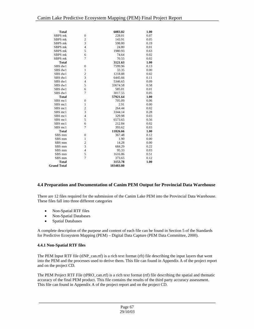
Canim Lake Predictive Ecosystem Mapping (PEM) Final Project Report
Page 67 29/10/03
Total 6083.82 1.00SBPS mk 0 228.01 0.07SBPS mk 2 143.91 0.05SBPS mk 3 598.80 0.19SBPS mk 4 24.80 0.01SBPS mk 5 1980.93 0.63SBPS mk 6 74.64 0.02SBPS mk 7 70.55 0.02
Total 3121.63 1.00SBS dw1 0 7599.96 0.13SBS dw1 1 33.35 0.00SBS dw1 2 1218.88 0.02SBS dw1 3 6445.66 0.11SBS dw1 4 5346.65 0.09SBS dw1 5 33674.58 0.58SBS dw1 6 585.01 0.01SBS dw1 7 3017.55 0.05
Total 57921.64 1.00SBS mc1 0 705.09 0.06SBS mc1 1 2.91 0.00SBS mc1 2 264.44 0.02SBS mc1 3 3344.14 0.28SBS mc1 4 329.98 0.03SBS mc1 5 6573.65 0.56SBS mc1 6 212.84 0.02SBS mc1 7 393.62 0.03
Total 11826.66 1.00SBS mm 0 367.48 0.12SBS mm 1 1.90 0.00SBS mm 2 14.28 0.00SBS mm 3 684.29 0.22SBS mm 4 95.33 0.03SBS mm 5 1616.86 0.51SBS mm 7 373.65 0.12
Total 3153.78 1.00Grand Total 183483.80
4.4 Preparation and Documentation of Canim PEM Output for Provincial Data Warehouse There are 12 files required for the submission of the Canim Lake PEM into the Provincial Data Warehouse. These files fall into three different categories
• Non-Spatial RTF files • Non-Spatial Databases • Spatial Databases
A complete description of the purpose and content of each file can be found in Section 5 of the Standards for Predictive Ecosystem Mapping (PEM) – Digital Data Capture (PEM Data Committee, 2000).
4.4.1 Non-Spatial RTF files The PEM Input RTF file (tINP_can.rtf) is a rich text format (rft) file describing the input layers that went into the PEM and the processes used to derive them. This file can found in Appendix A of the project report and on the project CD. The PEM Project RTF File (tPRO_can.rtf) is a rich text format (rtf) file describing the spatial and thematic accuracy of the final PEM product. This file contains the results of the third party accuracy assessment. This file can found in Appendix A of the project report and on the project CD.

Canim Lake Predictive Ecosystem Mapping (PEM) Final Project Report
Page 68 29/10/03
The PEM Knowledge Base RTF file (tKNB_can.rtf) is a rich text format (rtf) file describing the assumptions and structure of the model used to generate the PEM. This file can found in Appendix A of the project report and on the project CD. The PEM Structural Stage RTF file (tSTS_can.rtf) is a rich text format (rtf) file describing the input layers, assumptions, and structure of the model used to create the structural stage model.
4.4.2 Non-Spatial Databases The PEM Input Polygon Database (tINP_can.csv) is a comma separated value database file that describes significant information about the thematic input layers used in the PEM. This file can found in Appendix A of the project report and on the project CD. The PEM Project Database (tPRO_can.csv) is a comma separated value database file that listing the names of the various files submitted with the project. This file can found in Appendix A of the project report and on the project CD. The PEM Polygon Database (tECP_can.csv) is a comma separated value database file that contains the ecosystem attributes for the polygons found in the PEM Ecosystem Polygon Layer (tECP_can.E00). This file can found in Appendix F on the project CD. The PEM Structural Stage Database (tSTS_can.csv) is a comma separated value database file that contains the structural stage attributes for the structural stage polygons found in the structural stage layer (tSTS_can.E00). This file can found in Appendix F on the project CD. The PEM Sample Points Database (tECI_can.mdb) is a MS Access database containing the attributes for the plot data used in this project (tECI_can.e00). This file can found in Appendix F on the project CD.
4.4.3 Spatial Databases The PEM Polygon Coverage (tECP_can.e00) is a spatial coverage containing the PEM ecosystem polygons. This file is an Arc/Info Export format file that exports to the Arc/Info coverage format. This file can found in Appendix F on the project CD. The PEM Structural Stage Coverage (tSTS_can.e00) is a spatial coverage containing the structural stage polygons. This file is an Arc/Info Export format file that exports to the Arc/Info coverage format. This file can found in Appendix F on the project CD. The PEM Sample Points Coverage (tECI_can.e00) is a spatial coverage containing the sample point locations. This file is an Arc/Info Export format file that exports to the Arc/Info coverage format. This file can found in Appendix F on the project CD.

Canim Lake Predictive Ecosystem Mapping (PEM) Final Project Report
Page 69 29/10/03
5.0 Discussion The overall objective of the project was to produce a predictive ecosystem map (PEM) for a timber supply area (TSA) of operational interest to Weldwood of Canada Limited in the vicinity of Canim Lake using the LMES DSS methods. This overall objective was successfully achieved by the Canim Lake PEM Project. The specific sub-objectives were:
• To confirm the ability of the Digital Direct-to-Site-Series methods to produce accurate, cost-effective PEM maps for significant areas on an operational basis. • To verify costs, time requirements and expected levels of map accuracy for the Digital Direct-to-Site-Series procedures when applied on an operational basis.
• To produce a cost-effective predictive ecosystem map (PEM) for Weldwood of Canada Ltd’s TSA’s in the vicinity of Canim Lake (12, 1:20,000 map sheets) that will meet or exceed the provincial minimum required level of accuracy of 65%.
5.1 Applicability of the LMES DSS procedures at an operational scale In terms of the first sub-objective, the Canim Lake PEM project conclusively demonstrated that the LMES DSS procedures were scalable and could be applied to a significant area on an operational basis to produce a cost-effective PEM map of acceptable accuracy. Several challenges were encountered that related to scaling up of the LMES DSS procedures developed for the Cariboo PEM Pilot Project to apply to a full-size operational map area. The most significant was the realization that a single set of rules was often not able to be applied successfully to the entire extent of any large and topographically diverse BGC Sub-zone or variant. This issue was resolved by sub-dividing BGC Sub-zones into smaller and less diverse classification zones differentiated according to differences in size and scale of topographic relief and gross texture of the dominant parent material. Within these smaller and less diverse classification zones it was possible to apply a single set of classification rules. A positive side effect of this decision was that the fuzzy rule bases prepared for any given classification zone tended to be quite a bit smaller and more compact than equivalent rule bases that applied to an entire BGC Sub-zone. These smaller classification zone rule bases contained fewer classes that needed to be differentiated and were consequently easier to understand, revise and manage than larger rule files that had to differentiate a greater number of potential classes for an entire BGC Sub-zone or variant. A second issue related to scaling up was the physical size of raster data sets that are developed for very large areas. The LandMapR programs are limited by both available computer memory and by non-linear increases in processing time that effectively restrict processing to raster data sets that are not larger than about 4,000 rows by 4,000 columns. In fact, the optimum size of grid data sets for the LandMapR suite of programs was determined to be about 2,000 rows by 2,000 columns. For the present, this issue was resolved by developing procedures to sub-divide a single large, continuous raster data set for an entire map area of interest into a series of overlapping tiles with dimensions of less than 2,000 rows by 2,000 columns. In the case of the Canim Lake PEM, tiles were defined that fully enclosed a single 1:20,000 map sheet with the addition of a buffer of up to 1.5 km outside the margins of each 1:20,000 map sheet. Each tile was processed separately and independently. Edge effects were minimized by processing data for large overlap areas that were common to adjacent map sheets. In this way, grid cells located along the actual neat lines of map sheet boundaries tended to have virtually identical input data for adjacent map tiles so that the classifications applied to cells near map sheet boundaries were equivalent for cells in adjacent map tiles. Procedures were also developed to stitch individual map sheet tiles back together into a single complete and seamless mosaic for the entire map area of interest. The tiled mosaic contained no visible edge effects and no missing or incorrect classification data along map sheet margins. These procedures have been
Canim Lake Predictive Ecosystem Mapping (PEM) Final Project Report
Page 70 29/10/03
formalized into a series of database scripts that can be applied to sub-divide any large raster data set and then stitch data for individual tiles back together to form a single seamless mosaic for any area of interest.
5.2 Verification of costs, time requirements and expected levels of accuracy In terms of the second sub-objective, the Canim Lake PEM was able to successfully verify the costs, time requirements and expected levels of map accuracy for the LMES DSS procedures when applied on an operational basis. The Canim Lake PEM project demonstrated that costs for applying the LMES DSS procedures were controlled by the time and effort required for completing four main sets of activities. The first activity was obtaining, collating and registering all existing digital data sets and processing the DEM and other digital data layers to produce all of the input data layers required by the LMES DSS procedures. This can take from 2-3 days per map tile. The second, and most time consuming, activity was the creation and iterative revision of knowledge base rule tables. This activity was determined to require a total of about 5-7 working days per BGC Sub-zone or variant to complete. This included developing initial rule bases that achieved a “conceptual match”, revising the initial rule bases during and after a modeling workshop to achieve a better “geographic match” and finally applying revisions and fixes to produce several versions of “final” PEM maps. The third activity was applying the supposedly “final” rule bases to the data sets for the entire area to produce a PEM map for the entire area of interest that could be evaluated by the regional ecologist to identify any final concerns. Application of “final” rule bases to all required input data sets for an entire area of interest is actually not that time consuming. A set of 10-12 tiles can be fully processed to apply a new set of rules in about 12 hours. Experience in the Canim Lake PEM project showed that it is unrealistic to expect that this activity will only have to be done once for a truly “final” set of rules. It is more realistic to expect to process the entire data set 3-5 times to apply slightly refined rules meant to implement successive fixes for concerns that do not become apparent until final maps for the entire area of interest are prepared and reviewed. Realistically then, production of “final” grid maps for a full map area of 10-12 tiles will usually require about 3-5 days total time. The fourth main activity identified was that of creating a single seamless mosaic and of cleaning and filtering that mosaic to remove noise and undesirable detail to create a more cartographically tractable and visually appealing product. This activity is a necessary precursor to a final activity of preparing a final vector map for submission to the provincial digital data warehouse. As this was a new activity that had not previously been attempted by LMES, the time required to implement it this first time (10 days) is likely not representative of the time that will be required to implement in for subsequent projects. The Canim Lake PEM demonstrated that it was possible to produce a PEM for an operational area at a cost of not more than $0.45 per hectare. In fact, it was determined that costs could be related quite closely to the volume of data that had to be prepared and processed. The Canim Lake PEM was conducted using a 10 m grid size for all data sets, including the DEM. The area of interest was covered by 12 map sheet tiles of about 2,000 rows by 2,000 columns. If a future area of interest is described using grid data of a larger dimension (e.g. 25 m) it will be possible to process a larger area for an equivalent amount of effort and cost. The Canim Lake PEM permitted LandMapper to determine that costs per hectare could be effectively reduced to no more than $0.10 per hectare if 25 m grid data were used in place of 10 m grid data. Some costs, such as developing and revising rule bases, are fixed and are not subject to reduction with a change in grid size. Other costs, such as creating and processing data sets and creating and cleaning up final mosaic maps, are strongly related to grid dimensions as these control file size and processing times. LandMapper Environmental Solutions Inc. is confident that per hectare costs for full scale operational mapping utilizing grid data of 25 m grid size can be reduced to no more than $0.10 per hectare. The Canim Lake PEM was therefore very successful in determining that costs for full scale operational PEM mapping could be brought in at no more than $0.45 per hectare and could, in fact, be reduced to as low as $0.10 per hectare. The Canim Lake PEM provided an additional opportunity to test and document the level of accuracy that could be anticipated using the LMES DSS procedures, At the time of writing this report, initial results indicate that the overall average accuracy achieved by the Canim Lake PEM was 63% direct Site Series overlap in the small area test. This falls short of the desired level of accuracy of 65% but it is close.

Canim Lake Predictive Ecosystem Mapping (PEM) Final Project Report
Page 71 29/10/03
5.3 Meeting or exceeding the minimum required level of accuracy of 65% In terms of the third sub-objective, the Canim Lake PEM was not able to successfully demonstrate that the LMES DSS procedures could achieve the required minimum level of accuracy of 65% when applied on an operational basis. At the time this document was prepared, only provisional accuracy results were available for the Canim Lake PEM. These provisional results (Moon, 2003) indicated that the Canim Lake PEM had achieved an overall average accuracy of 63% percent exact overlap as measured by the small area test described by Moon (2003). This did not quite achieve the required provincial minimum level of accuracy of 65%, but it was very close. It can be expected, that once allowances for errors that arise from differences between essentially equivalent Site Series are factored into the accuracy analysis, the LMES DSS PEM maps will be deemed to have achieved at least 65% accuracy in the small area corridor analysis test. The small area corridor analysis test measures direct Site Series overlap within a narrow corridor that bounds each closed triangular transect used to collect field observations of actual recognized Site Series. The area of corridors along the closed, triangular accuracy transects tends to average about 5 ha, which was selected to correspond to the minimum size management area that can realistically expected to be mapped and managed at the specified mapping scale of 1:20,000. If the LMES DSS PEM maps achieve a minimum of 65% direct and equivalent Site Series overlap using this test, it can be assumed that they will be able to describe the proportional composition of any area on the map that is at least 5 hectares in size with at least a 65% level of accuracy. This should satisfy the provincial requirement for 65% accuracy for using the PEM maps for site index adjustments, which is the primary interpretive need for the Canim Lake PEM. The provisional results of accuracy analysis of the Canim Lake PEM did identify a concern with the level of accuracy achieved by the LMES DSS PEM maps using what is referred to as a polygon level analysis of accuracy. The preliminary results indicated that the LMES DSS PEM maps achieved only an average of 50% accuracy at the polygon level. The polygon level test of map accuracy compares the proportions of Site Series predicted to occur within each unique polygon on the LMES DSS PEM maps that is traversed in any part by an accuracy transect with the proportions of Site Series observed to occur along that portion of the transect that lies within the polygon. A very small corner of a large polygon can often end up being traversed by a small portion of an accuracy transect. The proportions of Site Series recorded along the portion of the accuracy transect that lies within a particular polygon are then compared to the proportions of Site Series that have been estimated to occur within the entire polygon and exact Site Series overlap is measured. This test assumes that the Site Series estimated to occur within each polygon occur in the specified proportions within every very small part of every polygon with no significant variation. This is very unlikely to ever be the case. Parts of a polygon may be Site Series 01 and other parts of the polygon may be Site Series 02, but every small area in the polygon cannot be expected to contain the same proportions of 01 and 02 as are used to describe the entire polygon area. In this sense, the transect corridor analysis method is somewhat inappropriate or unfair, as it does not provide a mechanism for obtaining a true sample of the entire range of variation within each full polygon for which an accuracy determination is made. It does not even guarantee that the proportions within some minimum sized portion of the polygon, of for example 5 ha, are assessed and compared to proportions determined for an equivalent minimum sized area by an accuracy transect. Questions about the relevance and usefulness of the polygon level analysis will have to be addressed before the LMES DSS PEM maps can be accepted by Timber Supply Branch for use in establishing Base Case timber supply estimates and revising annual allowable cut assessments. Considerable investigation and thought has gone into analyzing and attempting to understand the reasons why the LMES DSS PEM maps fail to achieve a higher level of accuracy at the polygon level. The key reason for the low level of polygon accuracy appears to be related to differences between the size, scale and accuracy with which the TRIM II DEM data portray the topographic surface and the actual size and scale of topographic features on the ground, as observed along accuracy transects and used by ecologists to assign field assessments of Site Series.
Canim Lake Predictive Ecosystem Mapping (PEM) Final Project Report
Page 72 29/10/03
The TRIM II DEM data are simply not able to capture and portray topographic features that are between 10 and 100 m in length and that correspond to micro to lower meso scale topographic variation. Having been collected at a grid interval of no smaller than 75 m and with a vertical accuracy of no better than 4-5 m, it is simply not possible for any DEM created from the TRIM II elevation data to accurately capture and portray topographic features that are shorter than about 100 m and that have a vertical expression of relief that is less than 5 m. It is clear that a significant amount of the local variation in Site Series classification, as determined in the field along accuracy transects, is related to short range variation in micro topography that is not captured and portrayed by the TRIM II DEM data. Moon (2003) observed frequent changes in the Site Series assigned along accuracy transects over distances of 10’s of meters. These changes in assigned Site Series were clearly related to local changes in site conditions that were very often related to small, subtle, local variations in micro-topography. The TRIM II DEM did not pick up these minor changes in topography correctly and so the Site Series classification at specific locations along accuracy transects is very often incorrect. It does appear, however, that the TRIM II DEM data can be useful and effective in two particular ways. In the first instance, the TRIM II DEM data are able to capture and portray longer range meso to macro scale topographic variation effectively and usefully. This longer range macro-topographic variation is responsible for some of the variation in ecological conditions and therefore in associated Site Series. The LMES DSS procedures that analyze the DEM data are able to extract some significant and useful information about likely site conditions. For instance, it is very possible to isolate large ridges from areas that are primarily upper to mid slopes from other areas that are primarily lower to toe slopes in the larger context. These macro topographic features do define zones of probability within which it is reasonable to expect to find a suite of ecological conditions and related Site Series that are, for example, drier than normal on the ridges and wetter than normal in the draws and toe slopes. The fact that the LMES DSS procedures are able to create PEM maps that achieve 63% exact Site Series overlap using the small area corridor analysis lends some credibility to the belief that some portion of the total variation in the spatial distribution of Site Series is explainable using analysis of available TRIM II DEM data. The macro-topographic variation captured by the TRIM II DEM data does permit definition of zones within which predominantly drier or wetter Site Series can be expected to occur. What the 10-25 m TRIM II DEM data are not able to do very effectively is to identify the exact site conditions (e.g. shape, landform position, moisture regime) at every small 5-10 m square location on the actual ground surface. These small variations in micro to meso scale topography give rise to local variations in site conditions that produce departures from the main expected Site Series within these broad zones where site conditions are expected to be somewhat drier or wetter than normal. Thus, it is both possible and expected that specific locations within these broad zones will exhibit Site Series that are different (drier or wetter) than the predominant Site Series expected to occur within that macro topographic zone. The second way in which the available TIM II DEM data appear to make a useful contribution is more difficult to explain and less certain to be understood correctly. It appears that the TRIM II DEM data act as a kind of sampling grid that, when superimposed onto the true landscape, produces a sort of systematic sample that provides information on the frequency, range and size of meso to micro scale topographic variation in the landscape. This sampling does not provide correct information on the exact locations of small local rises, dips or other topographic features, but it does provide a sort of estimate of how many rises and dips typically occur within a given area and the relative size (length and height) of these local features. Thus, while the DEM may not locate a particular knoll, ridge top, valley or depression in exactly the right place, it does provide some estimate of the proportion of the landscape in a particular area that is occupied by ridges, knolls, draws, depressions and similar features. These estimates of the proportions of the actual landscape that fall into drier landscape positions (knolls, ridges, etc.) and wetter landscape positions (draws, hollows, depressions) can prove to be both useful and meaningful. It has been suggested (Moon, 2003, personal communication) that, for any given area of some minimum size (e.g. 5 ha) this sampling can provide a fairly accurate estimate of the proportions of the area that are occupied by drier rises or wetter swales. These estimated proportions can be equated to estimates of the proportions of Site Series that are wetter or drier than normal for that particular maco-landform position as portrayed by the TRIM II DEM data. This may well explain why the LMES DSS estimates of proportions of Site Series achieve 63% accuracy in a small area corridor analysis but fail to achieve as high a level of accuracy in exact Site Series match at specific locations along an accuracy transect or within specific polygons on the polygon analysis.

Canim Lake Predictive Ecosystem Mapping (PEM) Final Project Report
Page 73 29/10/03
The TRIM II DEM data are not capable of portraying very small, local micro topographic features correctly and accurately. It is therefore not surprising that, when standing at a specific small location in the field, the LMES DSS maps may often classify the specific location incorrectly, because the DEM represents the location incorrectly. What is both somewhat surprising and encouraging is that the LMES DSS procedures, applied to the available TRIM II DEM data, do appear to provide reasonable estimates of the relative proportions of the main different Site Series within any minimum sized area for which the systematic sampling of the TRIM II DEM data supply an estimate of the proportions of the land surface that appear as higher and drier or lower and wetter. If it is sufficient that the LMES DSS PEM maps provide reliable estimates of the relative proportions of main Site Series within minimum sized areas of at least 5 hectares, then the available TRIM II DEM data appear to be able to support the required analysis and mapping. If it is deemed absolutely necessary that the LMES DSS PEM maps identify the correct Site Series at every specific point on the landscape, then the TRIM II DEM data will not be adequate and it would be necessary to obtain a DEM capable of capturing and portraying all small local micro-topographic variations of length 10 m or less and vertical heights of 1 m or less. This decision rests with the appropriate provincial authorities. For the present, at least, the Canim Lake PEM has shown what levels of accuracy it is possible to achieve using the available input data sets, particularly the TRIM II DEM data, and the LMES DSS procedures. It remains for the authorities and the client to decide whether the resulting maps are adequate for their purposes.
5.4 A final observation on how sampling error may have affected accuracy estimates The Canim Lake PEM accuracy assessment procedures conducted a very interesting and illuminating assessment of measurement error and how this may have affected assessments of map accuracy. As part of the Canim Lake PEM accuracy assessment procedures, four accuracy transects were selected which were all traversed by all four of the expert ecologists who were engaged to conduct the accuracy assessment protocol. All four ecologists followed exactly the same four traverses and each assigned their assessment of the correct Site Series along each segment of each transect. The ecologists conducted their traverses at different times and were not allowed to discuss their assessments or compare notes. A preliminary analysis of the accuracy data (Moon, 2003) indicated that the level of exact Site Series overlap agreement among the four ecologists was 65%. The level of agreement between the 4 different ecologists and the LMES DSS PEM map for the same four transects was also 65%. The accuracy assessment report indicated that, using the numbers alone, it was not possible to distinguish the estimates of proportions of Site Series obtained from the LMES DSS PEM map from the estimates provided by the four expert ecologists. This small test indicates that a large portion of the error that is assumed to be associated with the LMES PEM maps may well arise from measurement error in the accuracy transect data. One has to realize that in any classification system only a small proportion of the individuals assigned to a class are likely to be unambiguous members of that class. In practice, most individuals are intergrades between classes and only a limited numbers of individual sites represent classic examples of any class. Since most specific locations are likely to represent an intergrade between two or more defined classes, it then becomes a matter of opinion as to whether a specific location more correctly belongs to one class or an adjacent one. The results of the Canim Lake replication experiment clearly illustrate that even knowledgeable experts standing at exactly the same sites and observing exactly the same conditions are not likely to agree on the correct classification more than 65% of the time. Very slight differences in perception, opinion and experience will lead the experts to elect to place the exact same locations into different Site Series classes. It therefore becomes unreasonable to expect a PEM map, created without the advantage of being able to make site observations in the field, to agree with the Site Series classifications of an expert ecologist in the field at a rate that is any better than achieved in comparison to the classifications assigned by other experts who examined and classified the same sites in the field. It may well be that no PEM map will ever agree with an expert’s assessment of Site Series classes at a rate greater than 65%; if experts themselves cannot agree at a rate in excess of 65%.

Canim Lake Predictive Ecosystem Mapping (PEM) Final Project Report
Page 74 29/10/03
6.0 References Cited BC Forest Productivity Council, Site Productivity Working Group. June 2001. SIBEC Sampling and Data Standards, Version 5.1, Victoria, BC British Columbia Specifications and Guidelines for Geomatics Digital Orthophotos, Volume 7, Digital Orthophoto Specifications, Release 1.0, May 1997. Braumandl, T.F. and M. Curran, 1992. A Field Guide for Site Identification and Interpretation for the Nelson Forest Region. Land Management Handbook Number 29, BC Ministry of Forests. Victoria, BC. Coupé, R. and O. Steen 2003 (in progress) BEC Localization, Canim Lake Area. Unpublished map to BC Ministry of Forests, Cariboo Region. Ecological Data Committee, Ecosystems Working Group/Terrestrial Ecosystems Task Force for Resource Inventory Committee (RIC). 2000. Standards for Terrestrial Ecosystem Mapping (TEM) – Digital Data Capture in British Columbia. Ecosystem Technical Standards and Data Base Manual. Ecosystems Working Group. 1998. Standards for Terrestrial Ecosystems Mapping in British Columbia, Resource Inventory Committee (RIC), Victoria, BC. Eyton, J.R. 1991. Rate-of-change maps. Cartography and Geographic Information Systems 18: 87-103 Geological Survey of Canada. Map 1278A, Geology Bonaparte Lake British Columbia, 1971. Holland, Stuart S. 1976. Landforms of British Columbia A Physiographic Outline. British Columbia Department of Mines and Petrolium Resources, Bulletin 48. Howes, D.E. and E. Kenk (Version 2). 1997. Terrain Classification System for British Columbia, British Columbia Ministry of Environment, Manual 10. Ketcheson, M.V. and K.Lessard. 2003. Canim Lake BEC Localization Project Report. Unpublished report to Weldwood of Canada 100 Mile House Operations. Lloyd, D., K. Angrove, G. Hope, C. Thompson. 1990. A Guide to Site Identification and Interpretation for the Kamloops forest Region. Land Management Handbook Number 23. BC Ministry of Forests. Victoria, BC. MacMillan, R. A. 2002. Cariboo PEM Pilot: Documentation of methods and results for landform-based classification procedures. Prepared for the Cariboo Site Productivity Adjustment Working Group, Contract Number: SPAWG(3) and Lignum Limited, Williams Lake, BC. 80 pp. Meidinger, D. 2003. Protocol for Accuracy Assessment of Ecosystem Maps. Research Brach, BC Ministry of Forests, Victoria, BC. Moon, D. E. 2001. Predictive ecosystem mapping pilot: Project specifications, Cariboo Forest Region. Prepared for: The Cariboo Site Productivity Adjustment Working Group. Prepared by: CDT Core Decision Tech Inc. 17 pp. Moon, D. E., 2002, Cariboo PEM Pilot: Project Monitor’s Final Report. Submitted to the Cariboo Site Productivity Adjustment Working Group. CDT, Core Decision Technologies Inc. 49 pp. Moon, D. E. 2003. Canim Lake Predictive Ecosystem Mapping (PEM) Accuracy Assessment Report. In progress.

Canim Lake Predictive Ecosystem Mapping (PEM) Final Project Report
Page 75 29/10/03
PCI (V.8.0) Software Help. PEM Data Committee for the TEM Alternatives Task Force Resource Inventory Committee (RIC). 2000. Standards for Predictive Ecosystem Mapping -–Digital Data Capture. Predictive Ecosystem Technical Standards and Database Manual. Version 1.0. Victoria. BC Quinn, P., K. Beven, P. Chevallier and O. Planchon. 1991. The prediction of hillslope flow paths for distributed hydrological modelling using digital terrain models. Hydrological Processes. 5: 59-79 Robertson, T., K. Misurak, J. Shypitka, M. Ketcheson and V. Lipinski. 2002. Canim Lake PEM Surficial Material Thickness and Texture Terrain Mapping TRIM Sheets 93A.004, 93A.005, 93A.006, 93A.007, 93A.008, 92P.094, 92P.095, 92P.096, 92P.097, 92P.098, 92P.086, 92P.077. Final Report to Alan Hicks Weldwood of Canada Ltd.100 Mile House Operations. Steen, O.A. and R. A. Coupé, 1997. A field guide to forest site identification and interpretation for the Cariboo Forest Region. B.C. Min. For. Victoria, B.C. Land Manage. Handb. No. 39. Terrestrial Ecosystem Mapping Alternatives Task force for the Resources Inventory Committee. 1999. Standards for Predictive Ecosystem Mapping – Inventory Standard. Victoria, BC.