CANDLE: An Image Dataset for Causal Analysis in DisentangledRepresentations

Abbavaram Gowtham ReddyIIT Hyderabad, India

cs19resch11002@iith.ac.in

Benin Godfrey LIIT Hyderabad, India

benin.godfrey@cse.iith.ac.in

Vineeth N BalasubramanianIIT Hyderabad, Indiavineethnb@iith.ac.in

Abstract

Confounding effects are inevitable in real-world obser-vations. It is useful to know how the data looks like withoutconfounding. Coming up with methods that identify and re-move confounding effects are important for various down-stream tasks like classification, counterfactual data aug-mentation, etc. We develop an image dataset for CausalANalysis in DisentangLed rEpresentations(CANDLE). Wealso propose two metrics to measure the level of disentan-glement achieved by any model under confounding effects.We empirically analyze the disentanglement capabilities ofexisting methods on dSprites and CANDLE datasets.

1. IntroductionGround-truth causal information is needed for evalu-

ating models that learn causal effects from observationaldata [11]. Real-world datasets for such tasks are hardto obtain because of the fundamental problem of causalinference and the infeasility of randomized control trials.Therefore, we are constrained to use synthetic datasets andfew controlled real-world datasets [5], most of which arenon-image datasets. Also, synthetic datasets are hardlyrealistic and often favor granularity of variations ratherthan semantic constraints imposed by nature. We seekto fill the gap between semantic realism of typical im-age datasets and ground-truth data generation of simu-lated datasets. We develop a realistic, but simulated im-age dataset(Figure 1) for Causal ANalysis in DisentangLedrEpresentations(CANDLE), whose generation follows acausal graph with unobserved confounding effects, mimick-ing the real world.

We ask counterfactual questions on CANDLE to evalu-ate a model’s ability to learn the underlying causal structure.In few applications, generative factors are correlated due tophysical properties of nature(e.g., shadow and light posi-tion). But in many applications it is helpful to isolate thegenerative factors completely to understand various prop-erties of learned representations. Models that learn disen-tangled representations from confounded datasets are usefulfor learning representations from limited examples. Many

Figure 1: Sample images from CANDLE.

current models either assume confounding is not present, orignore it even if it is. We encourage models that considerconfounding by creating a dataset with both observed andunobserved confounding effects with complex background.The motivation to create a dataset in this fashion arose fromrecent ideas requiring weak supervision for reliable repre-sentation learning [9]. We also propose two metrics to eval-uate the level of disentanglement under confounding. Ex-isting metrics use generative factors and latent representa-tions to come up with disentanglement score. Our metricsconcentrate on the entire process of data generation, latentrepresentations and reconstructions. Our metrics are basedon the principles of causality and develops on the very littlework along this direction [14].

2. Related Work

There are several datasets available for causal inferenceand causal discovery [5] but they are non image datasets.Image datasets generated for causal analysis are studiedin disentangled representation learning(e.g., dSprites [12],MPI3D [4]). But CANDLE is unique such that it has com-plex backgrounds and object’s position is not fixed acrossimages making it challenging for models to learn disen-tangled representations. Currently various disentanglementmetrics are available(e.g., MIG [1], DCI [3], IRS [14]), butthey rely on the learned latent space to evaluate the disen-tangled representations and the effects of confounding arenot considered. IRS [14] considers the confounding effectto be present in the data generation mechanism but its im-plications were not considered while formulating the met-ric(e.g., two generative factors that are correlated can be en-

1

coded by a single latent factor but we like to penalise con-founded encodings). Since we are interested in counterfac-tual questions on confounded datasets, reconstructions areimportant.

3. The CANDLE DatasetCausal DAG G, based on which the dataset is gener-

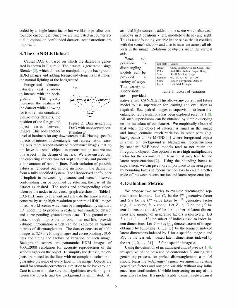
ated is shown in Figure 2. The dataset is generated usingsBlender [2], which allows for manipulating the backgroundHDRI images and adding foreground elements that inheritthe natural lighting of the background.

Figure 2: Data generatingDAG with unobserved con-founder(U).

Foreground elementsnaturally cast shadowsto interact with the back-ground. This greatlyincreases the realism ofthe dataset while allowingfor it to remain simulated.Unlike other datasets, theposition of the foregroundobject varies betweenimages. This adds anotherlevel of hardness for any downstream task. Having specificobjects of interest in disentanglement representation learn-ing puts more responsibility to reconstruct images that donot leave out small objects in reconstruction and we usethis aspect in the design of metrics. We also ensured thatthe capturing camera was not kept stationary and produceda fair amount of random jitter. Each variation of possiblevalues is rendered out as one instance in the dataset toform a fully specified system. The Unobserved confounderis implicit in between light source and scene, observedconfounding can be obtained by selecting the part of thedataset as desired. The nodes and corresponding valuestaken by the nodes in our causal graph are shown in Table 1.CANDLE aims to augment and alleviate the transferabilityconcerns by using high-resolution panoramic HDRI imagesof real-world scenes which can be manipulated by standard3D modelling to produce a realistic but simulated datasetand corresponding ground truth data. This ground-truthdata, though impossible to obtain in real-life, providevaluable information which can be exploited in variousmetrics of disentanglement. The dataset consists of 4050images as 320 × 240 png images and corresponding JSONfiles containing the factors of variation of each image.Background scenes are panoramic HDRI images of4000x2000 resolution for accurate reproduction of thescene’s lights on the object. To simplify the dataset, the ob-jects are placed on the floor with no complete occlusion toguarantee presence of every label in the image. Objects aresmall for semantic correctness in relation to the background.Care is taken to make sure that significant overlapping be-tween the objects and the background is eliminated. An

artificial light source is added to the scene which also castsshadows in 3 positions - left, middle(overhead) and right.This is a confounding variable in the sense that it conflictswith the scene’s shadow and also is invariant across all ob-jects in the image. Rotations of objects are in the verticalaxis.

Concepts ValuesObject Cube, Sphere, Cylinder, Cone, TorusColor Red, Blue, Yellow, Purple, OrangeSize Small, Medium, LargeRotation 0◦, 15◦, 30◦, 45◦, 60◦, 90◦

Scene Indoor, Playground, OutdoorLight Left, Middle, Right

Table 1: factors of variation

Weak su-pervision todisentanglingmodels can beprovided in avariety of ways.This variety ofsupervisionsare providednatively with CANDLE . This allows any current and futuremodel to use supervision for learning and evaluation asrequired. E.x. paired images as supervision to learn dis-entangled representations has been explored recently [10].All such supervisions can be obtained by simple queryingon the metadata of our dataset. We empirically observedthat when the object of interest is small in the imageand image contains much variation in other parts (e.g.background) unlike MPI3D [4] where foreground objectis small but background is black/plain, reconstructionsby standard VAE-based models tend to not retain theforeground objects. One option is to use high multiplicativefactor for the reconstruction term but it may lead to badlatent representations[7]. Using the bounding boxes assupervision, we can give more importance to the area givenby bounding boxes in reconstruction loss to create a bettertrade-off between reconstruction and latent representations.

4. Evaluation MetricsWe propose two metrics to evaluate disentangled rep-

resentation learners. Let Gi be the ith generative factorand Gik be the kth value taken by ith generative factor(e.g., i ∼ shape, k ∼ cone). Let Zj ∈ Z be the jth la-tent dimension and M,N be the number of latent dimen-sions and number of generative factors respectively. LetI ⊂ {1, 2, . . . ,M} be subset of indices used to index la-tent dimensions. Let D = {xi}Li=1 denote dataset of imagesobtained by following G. Let Zx

I be the learned, indexedlatent dimensions indexed by I for a specific image x andZx\I be the learned, indexed latent dimensions indexed by

the set {1, 2, . . . ,M} − I for a specific image x.Using the definition of disentangled causal process [14],

irrespective of the presence of confounder U during datagenerating process, for perfect disentanglement, a modelshould learn the independent causal mechanisms relatinggenerative factors and outcome variable without any influ-ence from confounders U while intervening on any of thegenerative factors. If a model is able to disentangle a causal

2

process for an outcome variable, we say that learnt latentspace is unconfounded. We call this phenomenon as Uncon-foundedness(UC). When the latent space is unconfounded,counterfactuals can be generated without any confoundingbias. We call this phenomenon as Counterfactual Genera-tiveness(CG). So, we look at causal disentanglement as thecombination of UC and CG.

4.1. Unconfoundedness(UC) Metric

The UC measure evaluates how well distinct generativefactors Gi are captured by different sets of latent dimen-sions ZI with no overlap. A seemingly related metric toUC is the DCI [3] metric. The D(disentanglement) scorein DCI metric is similar to UC metric but our analysis isbased on interventions and causal influences rather than cor-relation based models used for predicting Gi given Z. Alsothe way we compute UC metric is different (Equation 1).We assume that the variation in each Gi is captured by a setof latent dimensions ZI because of the fact that more thanone latent dimension can encode a single generative factor.For the simplicity of mathematical notation, we call Zx

I asQx

i . Now, if a model captures the underlying generativefactors Gi into a set of latent dimensions Qi, we define UCmeasure as

UC := 1− Ex∼D[ 1K

∑i 6=j

|Qxi ∩Qx

j ||Qx

i ∪Qxj |]

(1)

Where K =(N2

), the number of all possible pairs of gen-

erative factors. We are essentially finding Jaccard similar-ity coefficient among all possible pairs of latent sets corre-sponding to different generative factors to know how eachpair of generative factors are captured by unconfounded la-tent dimensions. If all the generative factors are disentan-gled into different sets of latent factors, we get UC = 1.In the worst case, if all generative factors share same set oflatents, we get UC = 0. To find ZI corresponding to Gi

we use IRS measure [14] because it is closely related to ourmetric and it works on the principles of interventions.

4.2. Counterfactual Generativeness(CG) Metric

When Gi’s are disentangled well, we can generate coun-terfactual images by intervening on any latent dimensionin the generative model without worrying about confound-ing bias. To define CG metric, we use Average Causal Ef-fect(ACE) and Individual Causal Effect(ICE)[13] of latentson generated images. Since latents in the generative modelare at the root level, conditioning is same as intervening.This lets us to define counterfactual generativeness (CG)measure as

CG := EI

[|ACEXcf

I

ZI−ACE

Xcf\I

Z\I|]

(2)

where XcfI represents the counterfactual image generated

when latent factors ZI are set to some interventional value.

ACEXcf

I

ZI, ACE

Xcf\I

Z\Iare defined to be the average causal

effects of ZI , Z\I on the respective counterfactual imageswhen the generative factor of interest is Gi. So, the CGmeasure calculates the normalized sum of differences of av-erage causal effects ofZI andZ\I on the generated counter-factual images. Since counterfactual outcomes with respectto a model can be generated through interventions, we ap-proximate ACE with average of ICEs over the dataset.Now CG metric is modified as follows.

CG := EI

[|ACEXcf

I

ZI−ACE

Xcf\I

Z\I|]

(3)

≈ 1

N

1

L

[|ICExcf

I

ZxI− ICE

xcf\I

Zx\I|]

(4)

ACE definition [13] is for real random variables, but ourtarget variable Xcf

I is an image, on which there is no clearway of defining causal effect of latents. For this work, we

define ICExcfI

ZxI

to be the difference in prediction probability

ofGik(of a pre-trained classifier) given xcfI generated whendo(ZI = Zx

I )(no change in latents of current example) andwhen do(ZI = baseline(Zx

I )). Mathematically,

ICExcfI

ZxI

= |P (Gik|xcfI , do(ZI = ZxI ))

− P (Gik|xcfI , do(ZI = baseline(ZI))|(5)

We choose to use baseline(ZxI ) = max dev(Zx

I , ZI).Where max dev(Zx

I , ZI) is the latent values that maxi-mally deviated from from current latent values Zx

I of aninstance x(taken over dataset) to ensure that we get rea-sonably different image than current image w.r.t generative

factor Gi. In the ideal scenario, ICExcfI

ZxI

is expected tooutput 1 because we are intervening on ZI correspondingto Gi(which is the prediction outcome in the classification

model) to generate counterfactual image. And ICExcf\I

Zx\I

isexpected to output 0 because we are intervening on Z\Ithat are not corresponding to Gi to generate counterfactualimage. For perfect disentanglement, CG = 1. For poordisentanglement, CG = 0.

5. Experiments

We use the following state of the art models in disentan-glement learning and corresponding semi supervised vari-ants to evaluate their ability to disentangle using our met-ric on CANDLE and dSprites: β-VAE [6], DIP-VAE [8],Factor-VAE [7] and β-TCVAE [1]. Models are comparedon IRS,UC and CG metrics.s ρ is the number of latentdimensions that we choose to attribute for each generativefactor.

3

CANDLE & dSprites: We chose a subset of CANDLEto mimic observable confounding effect. Confounding usedhere is that few objects appear in only few colors: cube inred and blue, sphere in blue and yellow, cylinder in yellowand purple, cone in purple and orange and torus in orangeand red. From the results it is evident that the models aregetting low UC and CG scores which reveal the need forbetter disentangled methods under confounding scenarios.Observe the relatively high(but not high enough for gooddisentanglement) UC and CG scores when ρ = 1 but whenρ = 2, we observe low UC and CG scores because mul-tiple latent dimensions are confounded and thus also affectreconstructions. Owing to the complex background, we ob-serve that models learn to reconstruct images with little tono information about the foreground object which leads tolow CG scores. In the table, ’SS’ refers to ’Semi Super-vised’. Accuracy of the trained model used in CG metric is98.9%. We can also use UC and CG to evaluate the modelsthat train on complete(no observed confounding) datasetslike dSprites. As we are training models on the full dSpritesdataset without any observable confounding effect, we ob-serve high UC score only when ρ = 1(Table 2). The reasonfor low score in CG is that models are not able to gener-ate reconstructions that capture difficult generative factorsexactly like angle, position, etc. Accuracy of the trainedmodel used in CG metric is 99.5%

Model IRS UC CG UC CGρ = 1 ρ = 1 ρ = 2 ρ = 2

CANDLEβ-VAE 0.80 0.40 0.21 0.13 0.20β-TCVAE 0.50 0.70 0.20 0.29 0.20DIP-VAE 0.24 0.40 0.13 0.29 0.14Factor-VAE 0.47 0.40 0.22 0.13 0.15SS-β-VAE 0.51 0.80 0.28 0.60 0.19SS-β-TCVAE 0.49 0.80 0.25 0.46 0.25SS-DIP-VAE 0.29 0.40 0.32 0.26 0.19SS-Factor-VAE 0.46 0.40 0.36 0.60 0.21

dSpritesβ-VAE 0.40 0.90 0.12 0.60 0.10β-TCVAE 0.62 0.90 0.12 0.60 0.13DIP-VAE 0.48 0.80 0.10 0.53 0.10Factor-VAE 0.52 0.90 0.14 0.60 0.14SS-β-VAE 0.55 0.90 0.16 0.30 0.15SS-β-TCVAE 0.70 0.90 0.15 0.33 0.14SS-DIP-VAE 0.24 0.40 0.08 0.13 0.06SS-Factor-VAE 0.47 0.90 0.15 0.33 0.14

Table 2: Comparison of IRS,UC and CG metrics onCANDLE & dSprites dataset for various models.

6. ConclusionWe introduced a dataset and two metrics to study the

level of unconfoundedness achieved by a model. Despiterepeated pivoting in the field of disentangled representa-tion learning and the possible unification with causal factorlearning or structure learning, we hope that this dataset andmetrics help the community in providing more challenging

and competing models in various tasks such as fairness, rea-soning, evaluation etc.

References[1] Ricky TQ Chen, Xuechen Li, Roger B Grosse, and David K

Duvenaud. Isolating sources of disentanglement in varia-tional autoencoders. In NeurIPS, 2018. 1, 3

[2] Blender Online Community. Blender - a 3d modelling andrendering package. http://www.blender.org. 2

[3] Cian Eastwood and Christopher KI Williams. A frameworkfor the quantitative evaluation of disentangled representa-tions. In ICLR, 2018. 1, 3

[4] Muhammad Waleed Gondal, Manuel Wuthrich, DjordjeMiladinovic, Francesco Locatello, Martin Breidt, ValentinVolchkov, Joel Akpo, Olivier Bachem, Bernhard Scholkopf,and Stefan Bauer. On the transfer of inductive bias from sim-ulation to the real world: a new disentanglement dataset. InNeurIPS, 2019. 1, 2

[5] Ruocheng Guo, Lu Cheng, Jundong Li, P. Richard Hahn, andHuan Liu. A survey of learning causality with data:problemsand methods. arXiv preprint arXiv:1809.09337, 2018. 1

[6] Irina Higgins, Loıc Matthey, Arka Pal, Christopher Burgess,Xavier Glorot, Matthew M Botvinick, Shakir Mohamed, andAlexander Lerchner. beta-vae: Learning basic visual con-cepts with a constrained variational framework. In ICLR,2017. 3

[7] Hyunjik Kim and Andriy Mnih. Disentangling by factoris-ing. arXiv preprint arXiv:1802.05983, 2018. 2, 3

[8] Abhishek Kumar, Prasanna Sattigeri, and Avinash Bal-akrishnan. Variational inference of disentangled latentconcepts from unlabeled observations. arXiv preprintarXiv:1711.00848, 2017. 3

[9] Francesco Locatello, Stefan Bauer, Mario Lucic, GunnarRaetsch, Sylvain Gelly, Bernhard Scholkopf, and OlivierBachem. Challenging common assumptions in the unsu-pervised learning of disentangled representations. In ICML,2019. 1

[10] Francesco Locatello, Ben Poole, Gunnar Ratsch, Bern-hard Scholkopf, Olivier Bachem, and Michael Tschannen.Weakly-supervised disentanglement without compromises.arXiv preprint arXiv:2002.02886, 2020. 2

[11] Christos Louizos, Uri Shalit, Joris M Mooij, David Sontag,Richard Zemel, and Max Welling. Causal effect inferencewith deep latent-variable models. In NeurIPS, 2017. 1

[12] Loic Matthey, Irina Higgins, Demis Hassabis, and AlexanderLerchner. dsprites: Disentanglement testing sprites dataset.https://github.com/deepmind/dsprites-dataset/, 2017. visited on 2020-08-01. 1

[13] J. Pearl. Causality. Cambridge University Press, 2009. 3[14] Raphael Suter, Djordje Miladinovic, Bernhard Scholkopf,

and Stefan Bauer. Robustly disentangled causal mecha-nisms: Validating deep representations for interventional ro-bustness. In ICML. PMLR, 2019. 1, 2, 3

4