Canberra, Australia

EFFECTS OF RANGING IN CIRCULAR POLARIZATION

John Luck and Chris MooreJohn-luck@bigpond.com , cmoore@eos-aus.com

MOTIVATION

It is all Dave Arnold’s fault!

He predicts that Laser Ranging to uncoated targets in CIRCULAR POLARIZATION will produce:

• Shorter ranges, by maybe 4 mm.• Greater return rates.• Reduced scatter.

He also predicts that, in LINEAR POLARIZATION, these quantities will be affected by the angle between the satellite velocity aberration vector and the direction of the polarization vector as it reaches the target.

We have conducted ranging experiments at Stromlo SLR, to see whether these effects can be detected. Some preliminary results were presented at the Grasse Workshop 2007.

MAIN EXPERIMENT

• A Quarter-Wave-Plate (QWP) was used to convert from linear to circular polarization.

• The QWP was mounted in a custom-built mechanical prototype “QWP INSERTER” and placed on the laser table in the Transmit Beam between the SHG and the Transmit/Receive Mirror.

• By remote control, the QWP was alternately inserted into, and withdrawn from, the laser path during ranging.

• This change of state occurred (generally) exactly on Normal Point bin boundaries. It took a couple of seconds, during which the laser was temporarily disabled.

• Processing, after standard filtering and trend removal, examined the differences between Normal Points in the two states.

• Have observed 2 LAGEOS-1, 2 LAGEOS-2 passes in Sep’07, and 1 ETS8 pass in Sep’08.

QWP INSERTER : EARLY PROTOTYPE

“OUT” of a laser path

QWP INSERTER: “IN”on laser table

QWP INSERTER: “OUT”

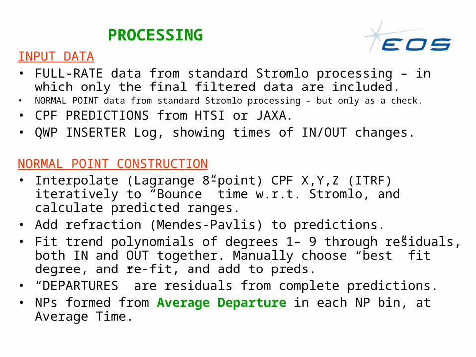
PROCESSINGINPUT DATA• FULL-RATE data from standard Stromlo processing – in which only the

final filtered data are included.• NORMAL POINT data from standard Stromlo processing – but only as a check.

• CPF PREDICTIONS from HTSI or JAXA.• QWP INSERTER Log, showing times of IN/OUT changes.

NORMAL POINT CONSTRUCTION• Interpolate (Lagrange 8-point) CPF X,Y,Z (ITRF) iteratively to “Bounce”

time w.r.t. Stromlo, and calculate predicted ranges.• Add refraction (Mendes-Pavlis) to predictions.• Fit trend polynomials of degrees 1– 9 through residuals, both IN and

OUT together. Manually choose “best” fit degree, and re-fit, and add to preds.

• “DEPARTURES” are residuals from complete predictions.• NPs formed from Average Departure in each NP bin, at Average Time.

JUDICIOUS USE OF STATISTICS

STATES: “IN” = CIRCULAR, “OUT” = LINEAR POLARIZATION

NORMAL POINT ANALYSIS• Used only “ADJACENT PAIRS” of NPs, i.e. discarded NPs not

having a neighbour of the opposite state on either side. This minimised external effects e.g. refraction anomalies, poor choice of trend function,…..

• Calculated Mean of NPs (a few numbers) and RMS about that Mean, separately for each state.

• Return Rates calculated only from “Adjacent Pairs” and best estimates of Number of Shots / NP bin.

FULL RATE ANALYSIS• Calculated Mean and RMS of FR data (thousands), separately for

each state.

“DEPARTURES” FROM TREND FUNCTIONETS-8, 11 Sep’08

ETS8 20080911 @ 09:00 Departures & NPsRefined Data, Poly Order 5, PolzVec

-150

-100

-50

0

50

100

150

39000 41000 43000 45000 47000 49000 51000

UTC seconds

Dep

artu

res

(pic

ose

cs)

Dep (IN)

DEP (OUT)

NPDep(IN)NPDep(OUT)

JUDICIOUS USE OF STATISTICS (cont.)

BOTH ANALYSES• Calculate Range Difference D between states:

D = MEAN IN – MEAN OUT – 3.1 pswhere 3.1 ps allows for thickness of QWP (1-way) got from catalogues: 1.8 mm.

• Calculate Pooled RMS S using classical formula given in textbooks when discussing Student’s ‘t’ application, e.g.

S=SQRT(s12/n2 + s2

2/n1) when n1, n2 large• Test H0: D = 0 against H1: D < 0 hence 1-tailed test, hence calc.

Student’s “t” = D/S with n1 + n2 - 2 degrees of freedom.• Calculate Variance Ratio F using classical formula given in

textbooks when discussing Fisher’s ‘F’ applications:

F = s12(IN)/s2

2(OUT) with n1-1, n2-1 degrees of freedom• Test H0: F = 1 against H1: F < 1 hence 1-tailed test.

(This test has very weak power when F ~ 1.)

JUDICIOUS USE OF STATISTICS (cont.)

• Comparison of Return Rates not statistically tested. ButB = [Acc.Returns/Num shots](IN) / [Acc.Returns/Num shots](OUT)using only numbers in Adjacent Pairs of NP bins.

• Confidence Level in following tables is[1 – Praccepting H1 when H0 is TRUE] x 100 %.

CONTRARY COMPARISON• An ordinary LAGEOS pass in which the QWP was never inserted,

was analysed to get a feeling for whether the procedure is valid. A dummy QWP log was constructed with random assignment of IN or OUT among NPs.

• In this pass, it is reasonable to suppose that the Null HypothesisH0: equality between “IN” (Circular) and “OUT” (Linear)will be accepted in all tests.

EXAMPLE: ETS-8 on 11 Sep’08

•

Statistic

NORMAL POINTS FULL RATE

IN OUT Comp IN vs OUT

IN OUT Comp IN vs OUT

Num.Obs 13 13 Diff 0 1431 1460 Diff 29

Mean Dep (ps) -1.9 1.7 Diff -3.1 -6.7 -2.7 2.6 Diff -3.1 -8.4

RMS (ps) 13.6 11.4 Pooled 4.9 47.5 48.1 Pooled 1.8

Student’s “t” d.f. 24 Diff / Pooled

-1.36 d.f. 2889 Diff / Pooled

-4.71

Confidence to reject equality of Means 90% 99.95%

Variance Ratio (Fisher’s “F”)

d.f. 12,12 OUT/ IN 1.43 d.f. Inf,Inf OUT/ IN 1.03

Confidence to reject equality of RMSs <90% >99.5%

Returns /shot (in Adj. Pairs) IN/ OUT 1.080

Return rate IN greater by: 8.0%

RESULTSTARGET LAG-1

8 Sep’07

LAG-19 Sep’07

LAG-211Sep’07

LAG-212 Sep’07

ETS-811 Sep’08

*LAG-2*10 Sep’08

Accepted Returns 3444 1934 2536 4298 2891 1323

Adj Normal Pts (C, L) 9, 9 8, 8 11, 11 12, 12 13, 13 8, 8

Diff of NP Means (ps) -2.9 -16.0 -7.1 -5.5 -6.7 +4.0

Conf.that Range C< L <65% > 95% > 95% > 95% > 95% 31%

Diff of FR Means (ps) -1.2 -10.7 -6.5 -4.7 -8.4 +5.4

Conf.that Range C< L <70% > 99.9% > 99.5% > 99.9% > 99.9% 1%

Ratio of NP RMSs 0.58 1.03 0.67 0.81 0.84 0.93

Conf.that RMS C< L 92% << 90% ~ 90% << 90% << 90% << 90%

Ratio of FR RMSs 0.95 1.01 1.05 1.04 0.99 1.05

Conf.that RMS C< L >99.5% 0 0 0 > 99.5% 0

Ratio Returns/Shot

C/ L 1.39 1.24 1.25 0.97 1.08

1.04

Circ. ratio greater by 39% 24% 25% -3% 8% 4%

CONCLUSIONS – MAIN EXPERIMENT

• There is statistical evidence that :

RANGE MEASUREMENTS ARE SHORTER IN CIRCULAR POLARIZATION than in Linear

seen more clearly in Full Rate analysis, although Normal Point analysis comes tantalizingly close to the same conclusion.

• There is :

NO EVIDENCE THAT RMS SCATTER IS SMALLER IN CIRCULAR POLARIZATION than in Linear.

(Using Fisher’s F-test with Full Rate data is meaningless!)• There is some evidence to suggest that, perhaps:

RETURN RATES ARE GREATER IN CIRCULAR POLARIZATION than in Linear.

ELECTRIC VECTOR ORIENTATION

• The orientation of the Electric Vector (EV) of Linearly Polarized Light has been mapped through the Stromlo SLR Coude path.

• The p- (parallel to plane of incidence) and s- (perpendicular) amplitude reflectances of each (plane) reflecting surface are taken into account, using data from handbooks, catalogues and text-books.

• Initial EV is vertically upwards, after the SHG (confirmed by EOS opticians), and is assigned a magnitude 1.

• Mapping ignores curved surfaces such as lenses, beam expanders and telescope primary and secondary mirrors (none of which are “turning mirrors”) so the output beam is as transmitted from the Tertiary Mirror.

ELECTRIC VECTOR ORIENTATION

• Calculations are done in local E,N,U coordinates and transformed to “Sky” coordinates after the tertiary mirror:

“Sky” = Magnitude, & Position Angle w.r.t Vertical Circle.

(E is the transmitted Electric Vector in E,N,U components)

Example: EV POSITION ANGLE (ψ)

Enhanced Aluminium (p = .967, s = -.990) for Coude mirrors, perfect for laser table mirrors.

ELECTRIC VECTOR POSITION ANGLEEnhanced Aluminium p = .967, s = -.990

-90-60-30

0306090

120150180210

0 30 60 90 120 150 180

Azimuth (degrees)

Pos'

n A

ngle

(deg

rees

) EL 00

EL 15

EL 30

EL 45

EL 60

EL 75

EL 90

DIFFERENCE IN POSITION ANGLEEnhanced Aluminium - "Perfect"

-3

-2

-1

0

1

2

3

4

0 30 60 90 120 150 180

Azimuth (degrees)

Pos

.Ang

. Dif

f (d

egre

es)

EL 00

EL 15

EL 30

EL 45

EL 60

EL 75

EL 90

Extreme Example: EV TRANSMITTED ENERGY

• Enhanced Aluminium (as in previous slide).• This sort of variation was measured at SGF 7840 last year and

reported at Grasse• When reflectances are equal or perfect, the variations disappear.

ELECTRIC VECTOR ENERGY / POWEREnhanced Aluminium p = .967, s = -.990

0.72

0.74

0.76

0.78

0.80

0.82

0.84

0.86

0 30 60 90 120 150 180

Azimuth (degrees)

Rel

ativ

e E

ner

gy

EL 00

EL 15

EL 30

EL 45

EL 60

EL 75

EL 90

VELOCITY ABERRATION VECTOR

V Satellite velocity vector, numerically differentiated in (rotating) ITRF from CPF predicted position vectors.

X Satellite geocentric position vector from CPF in ITRF

s Station geocentric position vector in ITRF

Ω Earth Rotation vector

R(φ,λ) Rotation from ITRF to Topocentric E, N, U

a Velocity aberration vector in E,N,U:

a = R(φ,λ) [V + Ω x (X – s)] as a unit vector

E Electric Vector (unit) expressed in E,N,U components

If θ is the angle between the plane of polarization and the velocity aberration at the satellite – the “ARNOLD ANGLE”, then:

θ = cos-1(a.b)

ARNOLD ANGLE

• Angle between polarization and aberration vectors calculated for one of the QWP LAGEOS-2 passes. It is not quite smooth ?

• For the ETS-8 pass, it is very nearly constant, at 122o.8• (but I have not yet worked out what to do with this information . . .)

L2 20070912 @ 07:40Angle between Vel.Aberr & Pol'zn Vectors

20

30

40

50

60

70

80

90

28000 28500 29000 29500 30000 30500 31000 31500 32000

UTC seconds

Arn

old

An

gle

(d

eg

ree

s)

PERILS OF NUMERICAL DIFFERENTIATION

• Essential to get BEST POSSIBLE TREND CURVE in this type of analysis, when looking for very small signals.

• Try to fit a physically meaningful function BEFORE fitting the final Trend Polynomial so that the polynomial is of lowest reasonable degree.

• Tried to fit empirical RANGE BIAS and TIME BIAS:

Obs(i) – Pred(i) = RB + Range_Rate(i)*TB• Tried to fit OSCULATING KEPLER ELEMENTS to the

predictions:

a, e, i, Ω, ω, t0 from X,Y,Z, Xdot, Ydot, Zdot

• They revealed DISCONTINUITIES in the RATES using Numerical Differentiation of CPF Positions (Lagr. Order 8)

RATE DISCONTINUITIES

• To make discontinuities visible, removed a line from the rates and took first differences.

• Rates calculated at time of each FR point in a STARLETTE pass.

STARLETTE 080910 @ 15:24Straightened RANGE RATES, Interpolation Order 8

0

2000

4000

6000

8000

10000

12000

142250 142300 142350 142400 142450 142500 142550 142600

UTC seconds (+86400)

Ran

ge

Rat

e (n

s/se

c)

ST 20080910 @ 15:24First Differences of Straightened Range Rates

Lagrange Numerical Differentiation Order 8

-1000-500

0500

10001500200025003000

142250 142300 142350 142400 142450 142500 142550 142600

UTC seconds (+86400)

Ran

ge

Rat

e D

iffs

(ns/

sec)

RATES OF CPF POSITIONS

• CONCLUSION: RATE DISCONTINUITIES EXIST IN CPF PREDICTIONS, which spoil efforts to find the best possible Trend Function.

ST 20080910 @ 15:24First Difference of Straightened Rates

Lagrange Numerical Differentiation Order 8

-25

-20

-15

-10

-5

0

5

10

142250 142300 142350 142400 142450 142500 142550 142600

UTC seconds (+86400)

X,Y

,Z R

ate

Dif

fss

(met

res/

sec)

Str.Xdot Diff

Str.Ydot Diff

Str.Zdot Diff

SUMMARY

• There is statistical evidence from ranging observations to support the prediction that RANGE MEASUREMENTS ARE SHORTER IN CIRCULAR POLARIZATION THAN IN LINEAR, by 1 mm or so.

• There is tantalizing evidence that RETURN RATES are GREATER in CIRCULAR POLARIZATION.

• There is little evidence that SCATTER is reduced.

• Imperfect p- and s-reflectances in Coude Path affect transmitted energy systematically in Az & El in LINEAR POLARIZATION.

• Angle between Velocity Aberration and Electric Vectors are readily calculated.

• CPF PREDICTIONS are subject to RATE DISCONTINUITIES.