Canadian Geotechnical Journal, Vol. 47, No. 7, pp. 791-805 ... · Canadian Geotechnical Journal,...
14
Canadian Geotechnical Journal, Vol. 47, No. 7, pp. 791-805, 2010 On the ”elastic” stiffness in a high-cycle accumulation model for sand: a comparison of drained and undrained cyclic triaxial tests T. Wichtmann i) ; A. Niemunis ii) ; Th. Triantafyllidis iii) Abstract High-cycle accumulation (HCA) models may be used for the prediction of settlements or stress relaxation in soils due to a large number (N> 10 3 ) of cycles with a relative small amplitude (ε ampl < 10 -3 ). This paper presents a discussion of the stiffness E used in the basic constitutive equation ˙ σ 0 = E : (˙ ε - ˙ ε acc - ˙ ε pl ) of a HCA model. E interrelates the ”trends” of stress and strain evolution. For the experimental assessment of the bulk modulus K =˙ u/ ˙ ε acc v the rate ˙ u of pore water pressure accumulation in undrained cyclic triaxial tests and the rate of volumetric strain accumulation ˙ ε acc v in drained cyclic tests have been compared. The pressure-dependent bulk modulus K was quantified from fifteen pairs of drained and undrained tests with different consolidation pressures and stress amplitudes. It is demonstrated that both the curves ε acc v (N ) in the drained tests and u(N ) in the undrained tests are well predicted by the author’s HCA model if the elastic stiffness is determined in a way described in the present paper. A simplified determination of K from the un- and reloading curve in an oedometric compression test is discussed. Key words: High-cycle accumulation model, stiffness E, bulk modulus K, stress relaxation, drained cyclic triaxial tests, undrained cyclic triaxial tests 1 Introduction A so-called high- or poly-cyclic loading, that means a load- ing with a large number of cycles (N> 10 3 ) and relative small strain amplitudes (ε ampl < 10 -3 ) is of practical rele- vance for many problems in geotechnical engineering. Ma- chine foundations are subjected to many small cycles with constant amplitude. The cyclic loading of the foundations of tanks, silos and watergates is caused by the changing height of the filling. Wind and wave loading causes a high- cyclic loading of the foundations of onshore- and offshore wind power plants. This loading may be multiaxial since the directions and frequencies of the wind and wave loading may be different. This topic is of high actuality for example in connection with a large number of offshore wind parks planned in the North Sea. Another example for a high- cyclic loading are foundations subjected to traffic loading (e.g. railways of high-speed trains or magnetic levitation trains). In that case the strain loops in the soil are also multiaxial due to the moving loads. A high-cyclic loading may not only cause an accumula- tion of permanent deformations (e.g. settlements) in the soil but it may also lead to residual changes of the average stress. For example, the shaft resistance of a pile in sand usually decreases with N because the normal stress act- ing on the shaft relaxates. If the sand is water-saturated i) Research Assistant, Institute of Soil Mechanics and Rock Me- chanics, University of Karlsruhe, Germany (corresponding author). Email: [email protected] ii) Research Assistant, Institute of Soil Mechanics and Rock Me- chanics, University of Karlsruhe, Germany iii) Professor and Director of the Institute of Soil Mechanics and Rock Mechanics, University of Karlsruhe, Germany and the cyclic loading is applied under nearly undrained conditions, then the pore water pressure accumulates and the mean effective stress p = tr(σ 0 )/3 decreases. In the extreme case the sand ”liquefies” (σ 0 = 0). The finite element (FE) method in combination with a special ”explicit” (N-type) calculation strategy (Section 2) and a high-cycle accumulation (HCA) model (Section 3) may be used to predict permanent deformations or stress relaxation due to a high-cyclic loading. The method may be used to solve the problems addressed above involving a high-cyclic loading. The basic assumption of the HCA model proposed by Niemunis et al. [4] is that the strain path and the stress path that result from a high-cyclic load- ing can be decomposed into an oscillating part and a trend. The oscillating part is described by the strain amplitude. The model predicts primarily the trend (accumulation) of strain ˙ ε acc . Depending on the boundary conditions, the cu- mulative trend can be observed both in the effective stress (pseudo-relaxation) and in strain (pseudo-creep). These trends are interrelated by ˙ σ 0 = E :(˙ ε - ˙ ε acc - ˙ ε pl ) (1) with the rate ˙ σ 0 of the effective stress σ 0 (compression pos- itive), the strain rate ˙ ε (compression positive), the given accumulation rate ˙ ε acc , a plastic strain rate ˙ ε pl (for stress paths touching the yield surface) and an elastic stiffness E. In the context of HCA models ”rate” means the derivative with respect to the number of cycles N (instead of time t), i.e. ˙ t = ∂ t /∂N . In this paper the total stress is denoted by σ = σ 0 + u1 with pore water pressure u. Note that the index t av for average (= trend) is omitted in this paper. A large number of drained cyclic element tests [10–14] has been performed on a medium coarse sand in order to 1
Transcript of Canadian Geotechnical Journal, Vol. 47, No. 7, pp. 791-805 ... · Canadian Geotechnical Journal,...
Canadian Geotechnical Journal, Vol. 47, No. 7, pp. 791-805, 2010
On the ”elastic” stiffness in a high-cycle accumulation model for sand: a
comparison of drained and undrained cyclic triaxial tests
T. Wichtmanni); A. Niemunisii); Th. Triantafyllidisiii)
Abstract
High-cycle accumulation (HCA) models may be used for the prediction of settlements or stress relaxation in soilsdue to a large number (N > 103) of cycles with a relative small amplitude (εampl < 10−3). This paper presents a discussion
of the stiffness E used in the basic constitutive equation σ′ = E : (ε − ε
acc − εpl) of a HCA model. E interrelates the
”trends” of stress and strain evolution. For the experimental assessment of the bulk modulus K = u/εaccv the rate u of
pore water pressure accumulation in undrained cyclic triaxial tests and the rate of volumetric strain accumulation εaccv in
drained cyclic tests have been compared. The pressure-dependent bulk modulus K was quantified from fifteen pairs ofdrained and undrained tests with different consolidation pressures and stress amplitudes. It is demonstrated that both thecurves εacc
v (N) in the drained tests and u(N) in the undrained tests are well predicted by the author’s HCA model if theelastic stiffness is determined in a way described in the present paper. A simplified determination of K from the un- andreloading curve in an oedometric compression test is discussed.
Key words: High-cycle accumulation model, stiffness E, bulk modulus K, stress relaxation, drained cyclic triaxial tests,undrained cyclic triaxial tests
1 Introduction
A so-called high- or poly-cyclic loading, that means a load-ing with a large number of cycles (N > 103) and relativesmall strain amplitudes (εampl < 10−3) is of practical rele-vance for many problems in geotechnical engineering. Ma-chine foundations are subjected to many small cycles withconstant amplitude. The cyclic loading of the foundationsof tanks, silos and watergates is caused by the changingheight of the filling. Wind and wave loading causes a high-cyclic loading of the foundations of onshore- and offshorewind power plants. This loading may be multiaxial sincethe directions and frequencies of the wind and wave loadingmay be different. This topic is of high actuality for examplein connection with a large number of offshore wind parksplanned in the North Sea. Another example for a high-cyclic loading are foundations subjected to traffic loading(e.g. railways of high-speed trains or magnetic levitationtrains). In that case the strain loops in the soil are alsomultiaxial due to the moving loads.
A high-cyclic loading may not only cause an accumula-tion of permanent deformations (e.g. settlements) in thesoil but it may also lead to residual changes of the averagestress. For example, the shaft resistance of a pile in sandusually decreases with N because the normal stress act-ing on the shaft relaxates. If the sand is water-saturated
i)Research Assistant, Institute of Soil Mechanics and Rock Me-chanics, University of Karlsruhe, Germany (corresponding author).Email: [email protected]
ii)Research Assistant, Institute of Soil Mechanics and Rock Me-chanics, University of Karlsruhe, Germany
iii)Professor and Director of the Institute of Soil Mechanics and RockMechanics, University of Karlsruhe, Germany
and the cyclic loading is applied under nearly undrainedconditions, then the pore water pressure accumulates andthe mean effective stress p = tr (σ′)/3 decreases. In theextreme case the sand ”liquefies” (σ′ = 0).
The finite element (FE) method in combination with aspecial ”explicit” (N-type) calculation strategy (Section 2)and a high-cycle accumulation (HCA) model (Section 3)may be used to predict permanent deformations or stressrelaxation due to a high-cyclic loading. The method maybe used to solve the problems addressed above involvinga high-cyclic loading. The basic assumption of the HCAmodel proposed by Niemunis et al. [4] is that the strainpath and the stress path that result from a high-cyclic load-ing can be decomposed into an oscillating part and a trend.The oscillating part is described by the strain amplitude.The model predicts primarily the trend (accumulation) ofstrain ε
acc. Depending on the boundary conditions, the cu-mulative trend can be observed both in the effective stress(pseudo-relaxation) and in strain (pseudo-creep). Thesetrends are interrelated by
σ′ = E : (ε − ε
acc − εpl) (1)
with the rate σ′ of the effective stress σ
′ (compression pos-itive), the strain rate ε (compression positive), the given
accumulation rate εacc, a plastic strain rate ε
pl (for stresspaths touching the yield surface) and an elastic stiffness E.In the context of HCA models ”rate” means the derivativewith respect to the number of cycles N (instead of time t),i.e. t = ∂ t /∂N . In this paper the total stress is denotedby σ = σ
′ + u1 with pore water pressure u. Note that theindex tav for average (= trend) is omitted in this paper.
A large number of drained cyclic element tests [10–14]has been performed on a medium coarse sand in order to
1
Wichtmann et al. Canadian Geotechnical Journal, Vol. 47, No. 7, pp. 791-805, 2010
develop suitable equations for εacc in Eq. (1). These equa-
tions are introduced in Section 3. The results from theaxisymmetric tests have been generalized to the full tenso-rial formulation of the HCA model. For the boundary valueproblems (BVPs) studied so far, the deformations were ofessential importance (e.g. FE calculations of settlementsof shallow foundations on dry sand [10]). Less attentionwas paid to an appropriate formulation of E, because theevolution of the trend of stress σ
′ was less important in theapplications considered first. However, for some BVPs con-siderable changes of the average stress are expected (e.g.piles under cyclic loading). A closer inspection of E be-comes necessary. It is the objective of the present paper.
At present a simple isotropic stiffness E = λ1 ⊗ 1 + 2µI
is used with the Lame-constants λ = Eν/(1 + ν)/(1 − 2ν)and µ = G = E/2/(1 + ν). The identity tensor I is definedas Iijkl = 1
2 (δikδjl + δilδjk) with Kronecker’s symbol δij .Therein E is Young’s modulus, G is the shear modulus andν is Poisson’s ratio. For Young’s modulus E, a pressure-dependent expression
E = A (patm)1−n (pav)n (2)
with the atmospheric pressure patm = 100 kPa and two di-mensionless positive constants A and n is used. Note thatE need not be hyperelastic contrary to the implicit mod-els for cyclic loading because it interrelates accumulationtrends and not stress and strain rates. The magnitude ofE has been roughly estimated.
No systematic experimental study of E in Eq. (1) can befound in the literature either. Some information about themagnitude of E can be found in the paper of Sawicki [6]. Hestudied pore pressure accumulation and liquefaction phe-nomena at the Izmit Bay coastal area (Turkey) during thestrong earthquake in August 1999. Sawicki used bulk mod-uli K between 145 and 156 MPa in his compaction model(for its critical review see [10]). These values were obtainedfrom the un- and reloading curves in oedometric tests. Saw-icki assumed that these values can be used for the ”elastic”stiffness in HCA models. Although being plausible, no ex-perimental evidence has been provided for this assumptionyet.
Assuming an isotropic E, the following questions may beposed:
• Which values of ν and E are adequate?
• Is E strongly pressure-dependent?
• Does E depend on amplitude and void ratio?
• For a simplified procedure, can E be determined fromthe un- and re-loading curve of an oedometric test oris it similar to a small-strain stiffness (i.e. attainablefrom a resonant column test or from wave velocity mea-surements)?
The present paper concentrates on K which influences therate of stress relaxation. Based on the results of 15 pairs ofdrained and undrained cyclic tests performed on a mediumcoarse sand the magnitude and the pressure-dependence ofK will be discussed. It will be shown that K is slightlyamplitude-dependent within the range of amplitudes stud-ied herein.
2 ”Explicit” calculation strategy
For predictions of permanent deformations or stress relax-ation due to cyclic loading by means of the finite element(FE) method, a conventional pure implicit calculation witha σ
′-ε constitutive model (e.g. elastoplastic multi-surfacemodels, endochronic models or hypoplastic models) is suit-able only for small numbers of cycles (N < 50). For largeN -values the numerical error becomes excessive in such cal-culations (Niemunis et al. [4]).
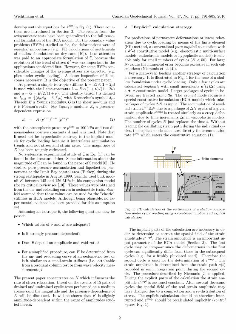
For a high-cyclic loading another strategy of calculationis necessary. It is illustrated in Fig. 1 for the case of a shal-low foundation under cyclic loading. Only a few cycles arecalculated implicitly with small increments σ
′(ε)∆t usinga σ
′-ε constitutive model. Larger packages of cycles in be-tween are treated explicitly. The explicit mode requires aspecial constitutive formulation (HCA model) which takespackages of cycles ∆N as input. The accumulation of resid-ual strain ε
acc∆N due to a package of ∆N cycles of a givenstrain amplitude εampl is treated similarly as a creep defor-mation due to time increments ∆t in viscoplastic models.The number of cycles N just replaces the time t. Withouttracing the oscillating strain path during the individual cy-cles, the explicit mode calculates directly the accumulationrate ε
acc which enters the constitutive equation (1).
�
t
F
t
� ampl
F
finite elements
implicit implicit
explicit explicit
control cycle
Fig. 1: FE calculation of the settlements of a shallow founda-tion under cyclic loading using a combined implicit and explicitcalculation
The implicit parts of the calculation are necessary in or-der to determine or correct the spatial field of the strainamplitude εampl. The strain amplitude is an important in-put parameter of the HCA model (Section 3). The firstcycle may be irregular since the deformations in the firstcycle can significantly differ from those in the subsequentcycles (e.g. for a freshly pluviated sand). Therefore thesecond cycle is used for the determination of εampl. Thestrain amplitude is determined from the strain path ε(t)recorded in each integration point during the second cy-cle. The procedure described by Niemunis [2] is applied.During the explicit parts of the calculation the strain am-plitude εampl is assumed constant. After several thousandcycles the spatial field of the real strain amplitude mayhave changed due to a compaction and a re-distribution ofstress. The explicit calculation should be therefore inter-rupted and εampl should be recalculated implicitly (controlcycles, Fig. 1).
2
Wichtmann et al. Canadian Geotechnical Journal, Vol. 47, No. 7, pp. 791-805, 2010
3 HCA model
For εacc in Eq. (1) the HCA model proposed by the authors
(Niemunis et al. [4]) uses
εacc = εacc m (3)
with the ”direction” of strain accumulation m =εacc/‖εacc‖ (flow rule, unit tensor) and the intensity εacc =
‖εacc‖. The flow rule of the modified Cam clay (MCC)model
m =
[
1
3
(
p − q2
M2p
)
1 +3
M2σ
′∗
]→
(4)
approximates well the ratios εaccv /εacc
q measured in drainedcyclic triaxial tests and has been adopted in the HCAmodel. For the triaxial case the Roscoe’s stress invariantsare p = (σ′
1 +2σ′
3)/3 and q = σ′
1 −σ′
3 with σ′
1 and σ′
3 beingthe axial and lateral effective stress components, respec-tively. The strain invariants are εv = ε1 + 2ε3 (volumetricstrain) and εq = 2/3(ε1−ε3) (deviatoric strain). For triax-ial extension η = q/p < 0 a small modification M = F Mc
is used in Eq. (4) to make it consistent with the Coulombcriterion:
F =
1 + Me/3 for η ≤ Me
1 + η/3 for Me < η < 01 for η ≥ 0
(5)
wherein
Mc =6 sinϕc
3 − sin ϕc
and Me = − 6 sin ϕc
3 + sinϕc
. (6)
In Eq. (4), t→ denotes Euclidean normalization and σ′∗ is
the deviatoric part of the effective stress.The intensity of strain accumulation εacc in Eq. (3) is
calculated as a product of six functions:
εacc = fampl fN fe fp fY fπ (7)
Each function (Table 1) takes into account a different influ-encing parameter. The function fampl describes the depen-dence of εacc on the strain amplitude εampl. Actually themodel incorporates a tensorial definition of the amplitudefor multidimensional strain loops [4]. It is applicable toconvex (e.g. elliptical) six-dimensional strain loops. Herewe use the scalar measure εampl of this tensorial ampli-tude only. A procedure to handle arbitrary six-dimensionalstrain loops using a spectral analysis has been proposed byNiemunis et al. [5]. The stress-dependence (the increase ofεacc with decreasing average mean pressure pav and withincreasing average stress ratio ηav = qav/pav) is capturedby the functions fp and fY while fe increases εacc with in-
creasing void ratio e. The function fN = fAN + fB
N (see Ta-ble 1) describes the dependence of εacc on cyclic preloading(historiotropy, fabric effects). The model counts the cyclesweighting their number with the amplitude. Such cyclicpreloading is quantified by
gA =
∫
fampl f AN dN (8)
and used in fN . For a constant amplitude the HCA modelpredicts accumulation curves εacc(N) proportional to fN =CN1[ln(1+CN2N)+CN3N ]. Physically gA can be seen as a
Function HCA model constants for Nmax =
105 200
fampl = min
(
εampl
εamplref
)Campl
100
εamplref
10−4
Campl 2.0 1.5
fN = fAN + fB
N CN1 3.6 · 10−4 1.97 · 10−4
fAN = CN1CN2 exp
[
−
gA
CN1fampl
]
CN2 0.43 0.24
fBN = CN1CN3 CN3 5.0 · 10−5 3.5 · 10−3
fp = exp
[
−Cp
(
pav
pref− 1
)]
Cp 0.43 0.025
pref 100 kPa
fY = exp(
CY Y av)
CY 2.0
fe =(Ce − e)2
1 + e
1 + eref(Ce − eref)
2Ce 0.54
eref 0.874
Table 1: Summary of the functions, reference quantities andconstants of the HCA model for a medium coarse sand; theconstants for Nmax = 105 were taken from [11], the constantsfor Nmax = 200 were derived in this study, Section 6
measure of the arrangement of grains rendering sand moreresistant against cyclic loading. The function fπ increasesthe accumulation rate due to changes of the polarization,see [4]. This function is not further used here since onlytests with a constant polarization have been performed (i.e.fπ = 1 holds). The constants of the HCA model for amedium coarse sand determined from drained tests withNmax = 105 cycles are summarized in the third column ofTable 1.
The multiplicative approach for εacc in Eq. (7) was cho-sen heuristically and then to some extent confirmed experi-mentally [10,11,13]. For example, fampl was found valid fortwo different average stresses, one with triaxial compression(pav = 200 kPa, ηav = 0.75) and the other one with triaxialextension (pav = 200 kPa, ηav = -0.5). The function fY
was confirmed for different average mean pressures 50 kPa≤ pav ≤ 300 kPa and the function fp was found valid fordifferent average stress ratios −0.5 ≤ ηav ≤ 1.313, althoughthe constants Cp and CY may slightly vary.
For axisymmetric element tests it is convenient to rewriteEq. (1) with Roscoe’s invariants:
p
q
=
K 0
0 3G
εv − εacc mv
εq − εacc mq
(9)
Omitting εpl in Eq. (1) is legitimate for homogeneous stress
fields. The bulk modulus K = E3(1−2ν) and shear modulus
G = E2(1+ν) are expected to be pressure-dependent. The
volumetric (mv) and the deviatoric (mq) portions of theflow rule are:
mv
mq
= 1√
1
3
(
p−q2
M2p
)
2
+6( q
M2 )2
p − q2
M2p
2q
M2
(10)
In a drained test with stress-controlled cycles, Eq. (10) cor-responds to the ratio of the rates of volumetric and devi-atoric strain predicted by the well-known formula of the
3
Wichtmann et al. Canadian Geotechnical Journal, Vol. 47, No. 7, pp. 791-805, 2010
MCC model:
εaccv
εaccq
=mv
mq
=M2 − (ηav)2
2ηav. (11)
4 Determination of elastic constants
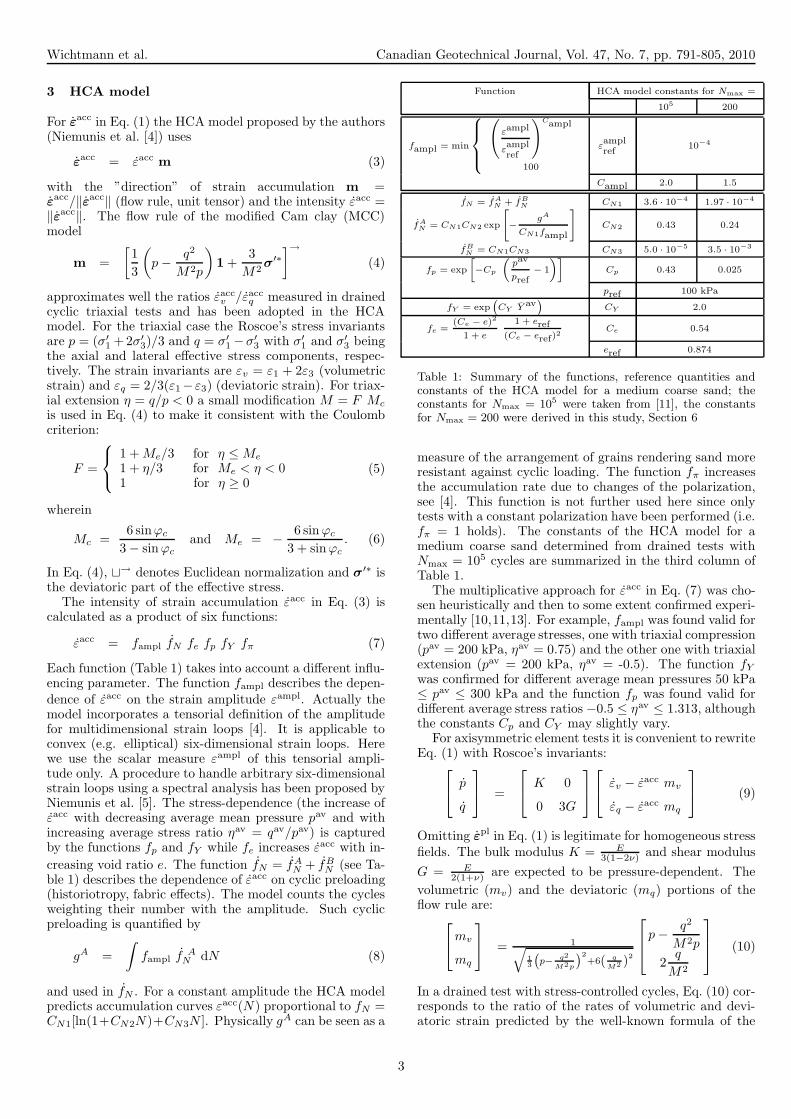
The bulk modulus K can be experimentally obtained froma comparison of the rate u of pore pressure accumulationin an undrained cyclic triaxial test and the rate εv of vol-umetric strain accumulation in a drained cyclic test withsimilar initial stress and initial void ratio and with the samecyclic loading. For an isotropic stress (q = 0, q = 0, mq =0) Eq. (9) takes either the form of isotropic relaxation (seethe average effective stress path in Fig. 2a)
p = −K εacc mv (12)
under undrained conditions (εv = 0) or the form of volu-metric creep
εv = εacc mv (13)
under drained conditions (p = 0). Comparing these equa-tions one may eliminate εacc mv and obtain
K = − p
εv
oru
εv
(14)
For a determination of Poisson’s ratio ν the effective stressevolution (p,q) observed in a strain-controlled undrainedcyclic triaxial test commenced at an anisotropic initialstress may be compared with the prediction of Eq. (9). Forεv = 0 and ε1 = 0 and therefore εq = 0 one obtains:
p
q
=
K 0
0 3G
−εacc mv
−εacc mq
(15)
The ratio of the relaxation rates
q
p=
3G
K
mq
mv
=9(1 − 2ν)
2(1 + ν)
2ηav
M2 − (ηav)2(16)
depends on ν. Stress paths for different ν-values are plottedexemplary in Fig. 2b. The stress relaxates until σ
′ = 0is reached. Note that the deviatoric relaxation q rapidlyincreases with stress ratio η = q/p. The Poisson’s ratio νcan be determined from the measured q/p or judged by acurve-fitting of the experimental data using Fig. 2b.
5 Tested material, test device, specimen prepara-tion procedure and testing program
The drained and the undrained cyclic tests were performedon a medium coarse quartz sand with subangular grainshape. The mean grain size and the coefficient of uniformityare d50 = 0.55 mm and Cu = d60/d10 = 1.8, respectively.The grain size distribution curve is given for example in [10](denoted as ”Sand No. 3”). The minimum and maximumvoid ratios emin = 0.577 and emax = 0.874 have been deter-mined according to German standard code DIN 18126.
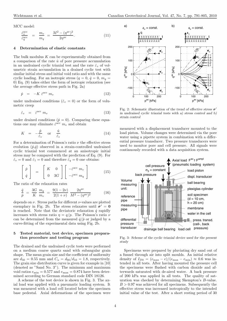
A scheme of the test device is shown in Fig. 3. The ax-ial load was applied with a pneumatic loading system. Itwas measured with a load cell located below the specimenbase pedestal. Axial deformations of the specimen were
Mc
qav [k
Pa]
pav [kPa]
CSL
CSL
σ'0
σ'0
b)
σ'0
σ'0
0 100 200
-100
0
100
200
qav [k
Pa]
pav [kPa]
CSL
CSL
0 100 200
-100
0
100
200
�
1
a)
σ'0
1
1
1
1
� = 0.4 0.3 0.2 0.1
� = 0.1 0.2 0.3 0.4
t
�
v = const.
t
�
v = const.
Me
Mc
Me
q
Fig. 2: Schematic illustration of the trend of effective stress σ′
in undrained cyclic triaxial tests with a) stress control and b)strain control
measured with a displacement transducer mounted to theload piston. Volume changes were determined via the porewater using a pipette system in combination with a differ-ential pressure transducer. Two pressure transducers wereused to monitor pore and cell pressure. All signals werecontinuously recorded with a data acquisition system.
load cell
displ. transducer
press. transd. (cell-, back pressure)
differential pressure transducer
back pressure
soil specimen (d = 10 cm, h = 20 cm)
drainage
Axial load Fav Fampl+ -
cell pressure σ3 = constant
(pneumatic loading system)
ball bearing
Volume measuring unit:
reference pipe
plexiglas cylinder
water in the cell
ball bearing
load piston
membranemeasuring pipe
Fig. 3: Scheme of the cyclic triaxial device used for the presentstudy
Specimens were prepared by pluviating dry sand out ofa funnel through air into split moulds. An initial relativedensity of ID0 = (emax − e)/(emax − emin) ≈ 0.6 was in-tended in all tests. After having mounted the pressure cellthe specimens were flushed with carbon dioxide and af-terwards saturated with de-aired water. A back pressureof 200 kPa was applied in all tests. The quality of sat-uration was checked by determining Skempton’s B-value.B > 0.97 was achieved for all specimens. Subsequently theeffective stress was increased isotropically to the intendedinitial value of the test. After a short resting period of 30
4
Wichtmann et al. Canadian Geotechnical Journal, Vol. 47, No. 7, pp. 791-805, 2010
minutes the cyclic axial loading was applied using a tri-angular load pattern. The cell pressure was kept constantduring the cycles.
In all tests (drained and undrained) the first cycle wasapplied under the drained condition. The first cycle maybe irregular and may generate much more deformation thanthe subsequent ones. The HCA model predicts only the ac-cumulation due to the subsequent regular cycles (see Figure1). In numerical calculations with the HCA model the firstcycle is calculated using a conventional implicit constiti-tutive model (we use for example hypoplasticity with in-tergranular strain [3,9]). Since the initial conditions at thebeginning of the regular cycles (initial stress and initial rela-tive density) were intended to be similar in the drained andin the undrained tests, the first cycle was applied drainedin both types of tests. In the undrained tests the drainagewas closed after the first cycle and all subsequent cycleswere applied undrained. The time period of a cycle wasT = 100 s. The first cycle is not included in the follow-ing evaluation of the ”elastic” stiffness E. In all diagramsN = 1 refers to the first regular cycle.
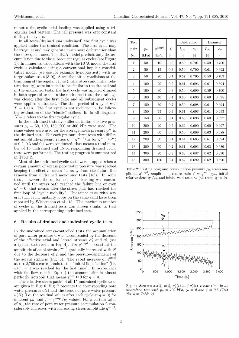
In the undrained tests five different initial effective pres-sures p0 = 50, 100, 150, 200 or 300 kPa were used. Thesame values were used for the average mean pressure pav inthe drained tests. For each pressure three tests with differ-ent amplitude-pressure ratios ζ = qampl/p0 (or qampl/pav)= 0.2, 0.3 and 0.4 were conducted, that means a total num-ber of 15 undrained and 15 corresponding drained cyclictests were performed. The testing program is summarizedin Table 2.
Most of the undrained cyclic tests were stopped when acertain amount of excess pore water pressure was reachedkeeping the effective stress far away from the failure line(known from undrained monotonic tests [15]). In sometests, however, the undrained cyclic loading was contin-ued until the stress path reached the failure line or evenσ
′ = 0, that means after the stress path had reached thefirst loop of ”cyclic mobility”. Undrained tests with sev-eral such cyclic mobility loops on the same sand have beenreported by Wichtmann et al. [15]. The maximum numberof cycles in the drained tests was chosen similar to thatapplied in the corresponding undrained test.
6 Results of drained and undrained cyclic tests
In the undrained stress-controlled tests the accumulationof pore water pressure u was accompanied by the decreaseof the effective axial and lateral stresses σ′
1 and σ′
3 (seea typical test result in Fig. 4). For qampl = constant the
amplitude of axial strain εampl1 gradually increased with N
due to the decrease of p and the pressure-dependence of
the secant stiffness (Fig. 5). The rapid increase of εampl1
at t ≈ 2,700 s corresponds to the ”initial liquefaction” (i.e.u/σ3 = 1 was reached for the first time). In accordancewith the flow rule in Eq. (4) the accumulation is almostperfectly isotropic that means εacc
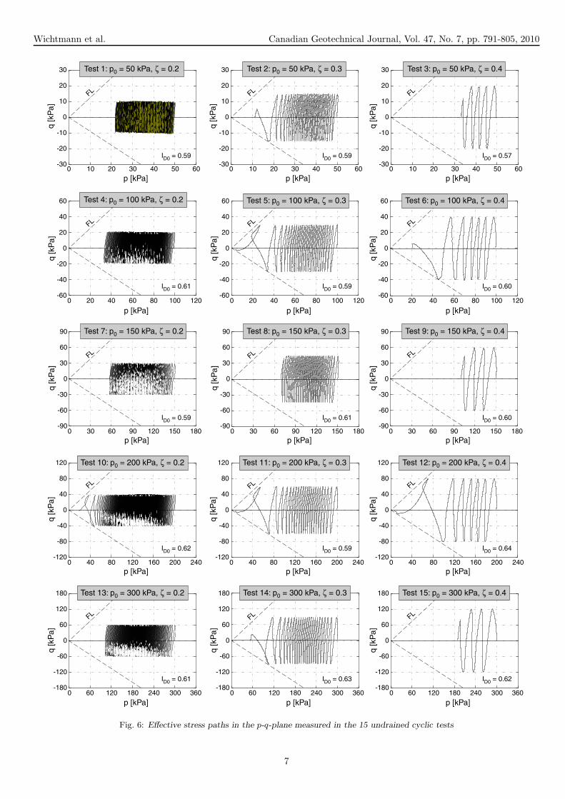
q ≈ 0 for q = 0.The effective stress paths of all 15 undrained cyclic tests
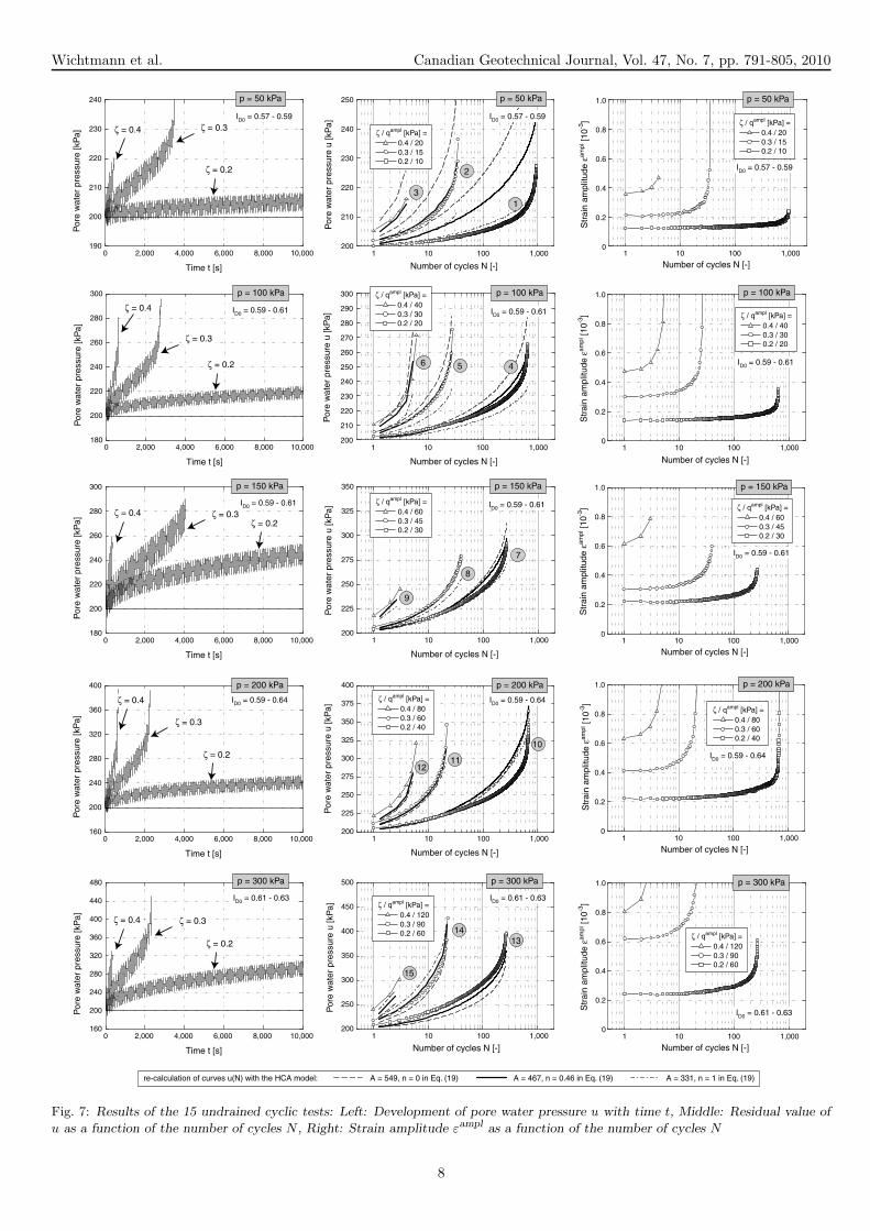
are given in Fig. 6. Fig. 7 presents the corresponding porewater pressures u(t) and the trends of pore water pressureu(N) (i.e. the residual values after each cycle at q = 0) fordifferent p0- and ζ = qampl/p0-values. For a certain valueof p0, the rate of pore water pressure accumulation u con-siderably increases with increasing stress amplitude qampl.
Test Undrained Drained
pair p0 qampl ζ ID0 e0 ID0 e0
No. [kPa] [kPa] [-] [-] [-] [-] [-]
1 50 10 0.2 0.59 0.701 0.59 0.700
2 50 15 0.3 0.59 0.700 0.61 0.692
3 50 20 0.4 0.57 0.705 0.58 0.703
4 100 20 0.2 0.61 0.693 0.61 0.694
5 100 30 0.3 0.59 0.699 0.59 0.700
6 100 40 0.4 0.60 0.696 0.60 0.695
7 150 30 0.2 0.59 0.698 0.61 0.694
8 150 45 0.3 0.61 0.693 0.61 0.693
9 150 60 0.4 0.60 0.696 0.60 0.697
10 200 40 0.2 0.62 0.690 0.60 0.697
11 200 60 0.3 0.59 0.699 0.63 0.688
12 200 80 0.4 0.64 0.685 0.61 0.694
13 300 60 0.2 0.61 0.693 0.63 0.686
14 300 90 0.3 0.63 0.687 0.62 0.690
15 300 120 0.4 0.62 0.692 0.62 0.690
Table 2: Testing program: consolidation pressure p0, stress am-
plitude qampl, amplitude-pressure ratio ζ = qampl/p0, initialrelative density ID0 and initial void ratio e0 (all tests: q0 = 0)
0 500 1,000 1,500 2,000 2,500 3,0000
50
100
150
200
250
300
350
Str
esse
s [k
Pa]
Time t [s]
σ3
u
σ1'
σ3'
Fig. 4: Stresses σ3(t), u(t), σ′
1(t) and σ′
3(t) versus time in anundrained test with p0 = 100 kPa, q0 = 0 and ζ = 0.3 (TestNo. 5 in Table 2)
5
Wichtmann et al. Canadian Geotechnical Journal, Vol. 47, No. 7, pp. 791-805, 2010
0 500 1,000 1,500 2,000 2,500 3,000-0.4
-0.3
-0.2
-0.1
0
0.1
0.2
0.3
0.4
Axi
al s
trai
n ε 1
[%]
Time t [s]
Fig. 5: Axial strain ε1(t) versus time in an undrained test withp0 = 100 kPa, q0 = 0 and ζ = 0.3 (Test No. 5 in Table 2)
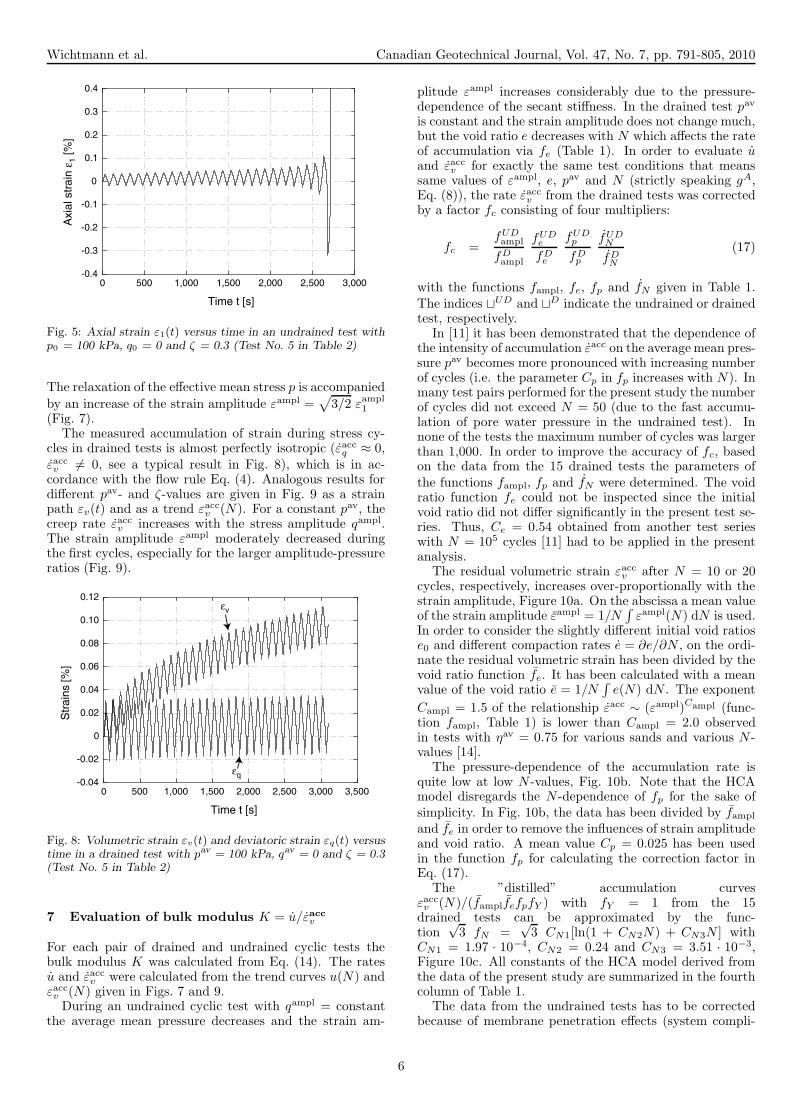
The relaxation of the effective mean stress p is accompanied
by an increase of the strain amplitude εampl =√
3/2 εampl1
(Fig. 7).The measured accumulation of strain during stress cy-
cles in drained tests is almost perfectly isotropic (εaccq ≈ 0,
εaccv 6= 0, see a typical result in Fig. 8), which is in ac-
cordance with the flow rule Eq. (4). Analogous results fordifferent pav- and ζ-values are given in Fig. 9 as a strainpath εv(t) and as a trend εacc
v (N). For a constant pav, thecreep rate εacc
v increases with the stress amplitude qampl.The strain amplitude εampl moderately decreased duringthe first cycles, especially for the larger amplitude-pressureratios (Fig. 9).
0 500 1,000 1,500 2,000 2,500 3,000 3,500-0.04
-0.02
0
0.02
0.04
0.06
0.08
0.10
0.12εv
εq
Str
ains
[%]
Time t [s]
Fig. 8: Volumetric strain εv(t) and deviatoric strain εq(t) versustime in a drained test with pav = 100 kPa, qav = 0 and ζ = 0.3(Test No. 5 in Table 2)
7 Evaluation of bulk modulus K = u/εacc
v
For each pair of drained and undrained cyclic tests thebulk modulus K was calculated from Eq. (14). The ratesu and εacc
v were calculated from the trend curves u(N) andεacc
v (N) given in Figs. 7 and 9.During an undrained cyclic test with qampl = constant
the average mean pressure decreases and the strain am-
plitude εampl increases considerably due to the pressure-dependence of the secant stiffness. In the drained test pav
is constant and the strain amplitude does not change much,but the void ratio e decreases with N which affects the rateof accumulation via fe (Table 1). In order to evaluate uand εacc
v for exactly the same test conditions that meanssame values of εampl, e, pav and N (strictly speaking gA,Eq. (8)), the rate εacc
v from the drained tests was correctedby a factor fc consisting of four multipliers:
fc =fUDampl
fDampl
fUDe
fDe
fUDp
fDp
fUDN
fDN
(17)
with the functions fampl, fe, fp and fN given in Table 1.The indices tUD and tD indicate the undrained or drainedtest, respectively.
In [11] it has been demonstrated that the dependence ofthe intensity of accumulation εacc on the average mean pres-sure pav becomes more pronounced with increasing numberof cycles (i.e. the parameter Cp in fp increases with N). Inmany test pairs performed for the present study the numberof cycles did not exceed N = 50 (due to the fast accumu-lation of pore water pressure in the undrained test). Innone of the tests the maximum number of cycles was largerthan 1,000. In order to improve the accuracy of fc, basedon the data from the 15 drained tests the parameters ofthe functions fampl, fp and fN were determined. The voidratio function fe could not be inspected since the initialvoid ratio did not differ significantly in the present test se-ries. Thus, Ce = 0.54 obtained from another test serieswith N = 105 cycles [11] had to be applied in the presentanalysis.
The residual volumetric strain εaccv after N = 10 or 20
cycles, respectively, increases over-proportionally with thestrain amplitude, Figure 10a. On the abscissa a mean valueof the strain amplitude εampl = 1/N
∫
εampl(N) dN is used.In order to consider the slightly different initial void ratiose0 and different compaction rates e = ∂e/∂N , on the ordi-nate the residual volumetric strain has been divided by thevoid ratio function fe. It has been calculated with a meanvalue of the void ratio e = 1/N
∫
e(N) dN . The exponent
Campl = 1.5 of the relationship εacc ∼ (εampl)Campl (func-tion fampl, Table 1) is lower than Campl = 2.0 observedin tests with ηav = 0.75 for various sands and various N -values [14].
The pressure-dependence of the accumulation rate isquite low at low N -values, Fig. 10b. Note that the HCAmodel disregards the N -dependence of fp for the sake ofsimplicity. In Fig. 10b, the data has been divided by fampl
and fe in order to remove the influences of strain amplitudeand void ratio. A mean value Cp = 0.025 has been usedin the function fp for calculating the correction factor inEq. (17).
The ”distilled” accumulation curvesεacc
v (N)/(famplfefpfY ) with fY = 1 from the 15drained tests can be approximated by the func-tion
√3 fN =
√3 CN1[ln(1 + CN2N) + CN3N ] with
CN1 = 1.97 · 10−4, CN2 = 0.24 and CN3 = 3.51 · 10−3,Figure 10c. All constants of the HCA model derived fromthe data of the present study are summarized in the fourthcolumn of Table 1.
The data from the undrained tests has to be correctedbecause of membrane penetration effects (system compli-
6
Wichtmann et al. Canadian Geotechnical Journal, Vol. 47, No. 7, pp. 791-805, 2010
0 10 20 30 40 50 60-30
-20
-10
00
10
20
30
q [k
Pa]
p [kPa]
q [k
Pa]
p [kPa]
q [k
Pa]
p [kPa]
q [k
Pa]
p [kPa]
q [k
Pa]
p [kPa]
0 10 20 30 40 50 60-30
-20
-10
0
10
20
30
q [k
Pa]
p [kPa]0 10 20 30 40 50 60
-30
-20
-10
10
20
30
q [k
Pa]
p [kPa]
Test 1: p0 = 50 kPa, ζ = 0.2 Test 2: p0 = 50 kPa, ζ = 0.3 Test 3: p0 = 50 kPa, ζ = 0.4
FL
Test 4: p0 = 100 kPa, ζ = 0.2
0 20 40 60 80 100 120
p [kPa]0 20 40 60 80 100 120
-60
-40
-20
0
20
40
60
q [k
Pa]
-60
-40
-20
0
20
40
60
p [kPa]0 20 40 60 80 100 120
q [k
Pa]
-60
-40
-20
0
20
40
60 Test 6: p0 = 100 kPa, ζ = 0.4Test 5: p0 = 100 kPa, ζ = 0.3
0 30 60 90 120 150 180-90
-60
-30
0
30
60
90 Test 9: p0 = 150 kPa, ζ = 0.4
q [k
Pa]
p [kPa]0 30 60 90 120 150 180
-90
-60
-30
0
30
60
90 Test 7: p0 = 150 kPa, ζ = 0.2
q [k
Pa]
p [kPa]0 30 60 90 120 150 180
-90
-60
-30
0
30
60
90 Test 8: p0 = 150 kPa, ζ = 0.3
0 40 80 120 160 200 240-120
-80
-40
0
40
80
120 Test 12: p0 = 200 kPa, ζ = 0.4
q [k
Pa]
p [kPa]0 40 80 120 160 200 240
-120
-80
-40
0
40
80
120 Test 10: p0 = 200 kPa, ζ = 0.2
q [k
Pa]
p [kPa]0 40 80 120 160 200 240
-120
-80
-40
0
40
80
120 Test 11: p0 = 200 kPa, ζ = 0.3
0 60 120 180 240 300 360-180
-120
-60
0
60
120
180 Test 15: p0 = 300 kPa, ζ = 0.4
q [k
Pa]
p [kPa]0 60 120 180 240 300 360
-180
-120
-60
0
60
120
180 Test 13: p0 = 300 kPa, ζ = 0.2
q [k
Pa]
p [kPa]0 60 120 180 240 300 360
-180
-120
-60
0
60
120
180 Test 14: p0 = 300 kPa, ζ = 0.3
ID0 = 0.59 ID0 = 0.59 ID0 = 0.57
ID0 = 0.61 ID0 = 0.59 ID0 = 0.60
ID0 = 0.59 ID0 = 0.61 ID0 = 0.60
ID0 = 0.62 ID0 = 0.59 ID0 = 0.64
ID0 = 0.61 ID0 = 0.63 ID0 = 0.62
FL FL
FL FL FL
FL FL FL
FL FL FL
FL FL FL
Fig. 6: Effective stress paths in the p-q-plane measured in the 15 undrained cyclic tests
7
Wichtmann et al. Canadian Geotechnical Journal, Vol. 47, No. 7, pp. 791-805, 2010
1 10 100 1,000200
250
300
350
400
450
500
Por
e w
ater
pre
ssur
e u
[kP
a]
Number of cycles N [-]
ζ / qampl [kPa] =
0.2 / 60 0.3 / 90 0.4 / 120
ID0 = 0.61 - 0.63
1 10 100 1,000200
210
220
230
240
250
Por
e w
ater
pre
ssur
e u
[kP
a]
Number of cycles N [-]
ζ / qampl [kPa] =
0.2 / 10 0.3 / 15 0.4 / 20
ID0 = 0.57 - 0.59
1 10 100 1,000200
210
220
230
240
250
260
270
280
290
300
Por
e w
ater
pre
ssur
e u
[kP
a]
Number of cycles N [-]
ζ / qampl [kPa] =
0.2 / 20 0.3 / 30 0.4 / 40
ID0 = 0.59 - 0.61
1 10 100 1,000200
225
250
275
300
325
350
Por
e w
ater
pre
ssur
e u
[kP
a]
Number of cycles N [-]
ζ / qampl [kPa] =
0.2 / 30 0.3 / 45 0.4 / 60
ID0 = 0.59 - 0.61
1 10 100 1,000200
225
250
275
300
325
350
375
400
Por
e w
ater
pre
ssur
e u
[kP
a]
Number of cycles N [-]
ζ / qampl [kPa] =
0.2 / 40 0.3 / 60 0.4 / 80
ID0 = 0.59 - 0.64
p = 50 kPa
p = 100 kPa
p = 150 kPa
p = 200 kPa
p = 300 kPa
0 2,000 4,000 6,000 8,000 10,000190
200
210
220
230
240
Por
e w
ater
pre
ssur
e [k
Pa]
Time t [s]
0 2,000 4,000 6,000 8,000 10,000180
200
220
240
260
280
300
Por
e w
ater
pre
ssur
e [k
Pa]
Time t [s]
0 2,000 4,000 6,000 8,000 10,000180
200
220
240
260
280
300
Por
e w
ater
pre
ssur
e [k
Pa]
Time t [s]
0 2,000 4,000 6,000 8,000 10,000160
200
240
280
320
360
400
Por
e w
ater
pre
ssur
e [k
Pa]
Time t [s]
0 2,000 4,000 6,000 8,000 10,000160
200
240
280
320
360
400
440
480
Por
e w
ater
pre
ssur
e [k
Pa]
Time t [s]
ζ = 0.2
ζ = 0.3ζ = 0.4
ζ = 0.2
ζ = 0.3
ζ = 0.4
ζ = 0.2ζ = 0.3ζ = 0.4
ζ = 0.2
ζ = 0.3
ζ = 0.4
ζ = 0.2
ζ = 0.3ζ = 0.4
p = 50 kPa
p = 100 kPa
p = 150 kPa
p = 200 kPa
p = 300 kPa
ID0 = 0.61 - 0.63
ID0 = 0.59 - 0.64
ID0 = 0.59 - 0.61
ID0 = 0.59 - 0.61
ID0 = 0.57 - 0.59
1 10 100 1,0000
0.2
0.4
0.6
0.8
1.0
Str
ain
ampl
itude
εam
pl [1
0-3]
Number of cycles N [-]
ζ / qampl [kPa] =
0.2 / 10 0.3 / 15 0.4 / 20
ID0 = 0.57 - 0.59
1 10 100 1,000
Number of cycles N [-]
0
0.2
0.4
0.6
0.8
1.0
Str
ain
ampl
itude
εam
pl [1
0-3] ζ / qampl [kPa] =
0.2 / 20 0.3 / 30 0.4 / 40
ID0 = 0.59 - 0.61
1 10 100 1,000
Number of cycles N [-]
0
0.2
0.4
0.6
0.8
1.0
Str
ain
ampl
itude
εam
pl [1
0-3]
Str
ain
ampl
itude
εam
pl [1
0-3]
ζ / qampl [kPa] =
0.2 / 30 0.3 / 45 0.4 / 60
ID0 = 0.59 - 0.61
1 10 100 1,000
Number of cycles N [-]
0
0.2
0.4
0.6
0.8
1.0
ζ / qampl [kPa] =
0.2 / 40 0.3 / 60 0.4 / 80
ID0 = 0.59 - 0.64
1 10 100 1,000
Number of cycles N [-]
0
0.2
0.4
0.6
0.8
1.0
Str
ain
ampl
itude
εam
pl [1
0-3]
ζ / qampl [kPa] =
0.2 / 60 0.3 / 90 0.4 / 120
ID0 = 0.61 - 0.63
p = 50 kPa
p = 100 kPa
p = 150 kPa
p = 200 kPa
p = 300 kPa
3
2
1
6 5 4
9
8
7
1211
10
15
1413
re-calculation of curves u(N) with the HCA model: A = 549, n = 0 in Eq. (19) A = 467, n = 0.46 in Eq. (19) A = 331, n = 1 in Eq. (19)
Fig. 7: Results of the 15 undrained cyclic tests: Left: Development of pore water pressure u with time t, Middle: Residual value of
u as a function of the number of cycles N , Right: Strain amplitude εampl as a function of the number of cycles N
8
Wichtmann et al. Canadian Geotechnical Journal, Vol. 47, No. 7, pp. 791-805, 2010
1 10 100 1,000 1 10 100 1,000
Number of cycles N [-]
0
0.2
0.4
0.6
0.8
1.0
Str
ain
ampl
itude
εam
pl [1
0-3]
ζ / qampl [kPa] =
0.2 / 10 0.3 / 15 0.4 / 20
ID0 = 0.58 - 0.61
1 10 100 1,000
Number of cycles N [-]
0
0.2
0.4
0.6
0.8
1.0
Str
ain
ampl
itude
εam
pl [1
0-3]
ζ / qampl [kPa] =
0.2 / 20 0.3 / 30 0.4 / 40
ID0 = 0.59 - 0.61
1 10 100 1,000
Number of cycles N [-]
0
0.2
0.4
0.6
0.8
1.0
Str
ain
ampl
itude
εam
pl [1
0-3]
ζ / qampl [kPa] =
0.2 / 30 0.3 / 45 0.4 / 60
ID0 = 0.60 - 0.61
1 10 100 1,000
Number of cycles N [-]
0
0.2
0.4
0.6
0.8
1.0
Str
ain
ampl
itude
εam
pl [1
0-3] ζ / qampl [kPa] =
0.2 / 40 0.3 / 60 0.4 / 80
ID0 = 0.60 - 0.63
1 10 100 1,000
Number of cycles N [-]
0
0.2
0.4
0.6
0.8
1.0
Str
ain
ampl
itude
εam
pl [1
0-3]
ζ / qampl [kPa] =
0.2 / 60 0.3 / 90 0.4 / 120
ID0 = 0.62 - 0.63
p = 50 kPa
p = 100 kPa
p = 150 kPa
p = 200 kPa
p = 300 kPa
-0.02
0
0.02
0.04
0.06
0.08
0.10
0.12
0.14
0
0.04
0.08
0.12
0.16
0.20
0 2,000 4,000 6,000 8,000 10,000
0
0.04
0.08
0.12
0.16
Time t [s]
0 2,000 4,000 6,000 8,000 10,000
Time t [s]
0 2,000 4,000 6,000 8,000 10,000
Time t [s]
0 2,000 4,000 6,000 8,000 10,000
0
0.04
0.08
0.12
0.16
0.20
0.24
Time t [s]
0 2,000 4,000 6,000 8,000 10,000
0
0.04
0.08
0.12
0.16
0.20
0.24
0.28
Vol
umet
ric s
trai
n ε v
[%]
Vol
umet
ric s
trai
n ε v
[%]
Vol
umet
ric s
trai
n ε v
[%]
Vol
umet
ric s
trai
n ε v
[%]
Vol
umet
ric s
trai
n ε v
[%]
Time t [s]
p = 300 kPa
ID0 = 0.62 - 0.63
ζ = 0.2ζ = 0.3
ζ = 0.4
ζ = 0.4
ζ = 0.4
ζ = 0.3
ζ = 0.3
ζ = 0.2
ζ = 0.2
ζ = 0.4
ζ = 0.3
ζ = 0.3
ζ = 0.4
ζ = 0.2
p = 200 kPa
ID0 = 0.60 - 0.63
p = 150 kPa
ID0 = 0.60 - 0.61
p = 100 kPa
ID0 = 0.59 - 0.61
ζ = 0.2
p = 50 kPa
ID0 = 0.58 - 0.61
0
0.02
0.04
0.06
0.08
0.10
0.12
0.14
0.16
Number of cycles N [-]
Res
idua
l vol
. str
ain
εacc [%
]v
ζ / qampl [kPa] =
0.2 / 10 0.3 / 15 0.4 / 20
ID0 = 0.58 - 0.61
1 10 100 1,000
Number of cycles N [-]
Res
idua
l vol
. str
ain
εacc [%
]v
ζ / qampl [kPa] =
0.2 / 20 0.3 / 30 0.4 / 40
ID0 = 0.59 - 0.61
1 10 100 1,0000
0.02
0.04
0.06
0.08
0.10
0.12
0.14
0.16
0.18
0.20
Number of cycles N [-]
Res
idua
l vol
. str
ain
εacc [%
]v
ζ / qampl [kPa] =
0.2 / 30 0.3 / 45 0.4 / 60
ID0 = 0.60 - 0.61
1 10 100 1,0000
0.02
0.04
0.06
0.08
0.10
0.12
0.14
0.16
0.18
0.20
Number of cycles N [-]
Res
idua
l vol
. str
ain
εacc [%
]v
ζ / qampl [kPa] =
0.2 / 40 0.3 / 60 0.4 / 80
ID0 = 0.60 - 0.63
1 10 100 1,0000
0.05
0.10
0.15
0.20
0.25
0.30
Number of cycles N [-]
ζ / qampl [kPa] =
0.2 / 60 0.3 / 90 0.4 / 120
ID0 = 0.62 - 0.63
Res
idua
l vol
. str
ain
εacc [%
]v
p = 50 kPa
p = 100 kPa
p = 150 kPa
p = 200 kPa
p = 300 kPa
3
2
1
0
0.02
0.04
0.06
0.08
0.10
0.12
0.14
0.16
6
5
4
98
7
12
11
10
15
1413
re-calculation with HCA model
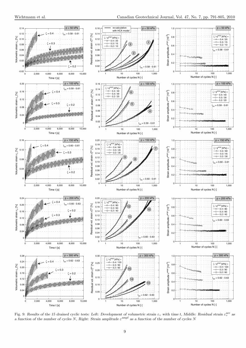
Fig. 9: Results of the 15 drained cyclic tests: Left: Development of volumetric strain εv with time t, Middle: Residual strain εaccv as
a function of the number of cycles N , Right: Strain amplitude εampl as a function of the number of cycles N
9
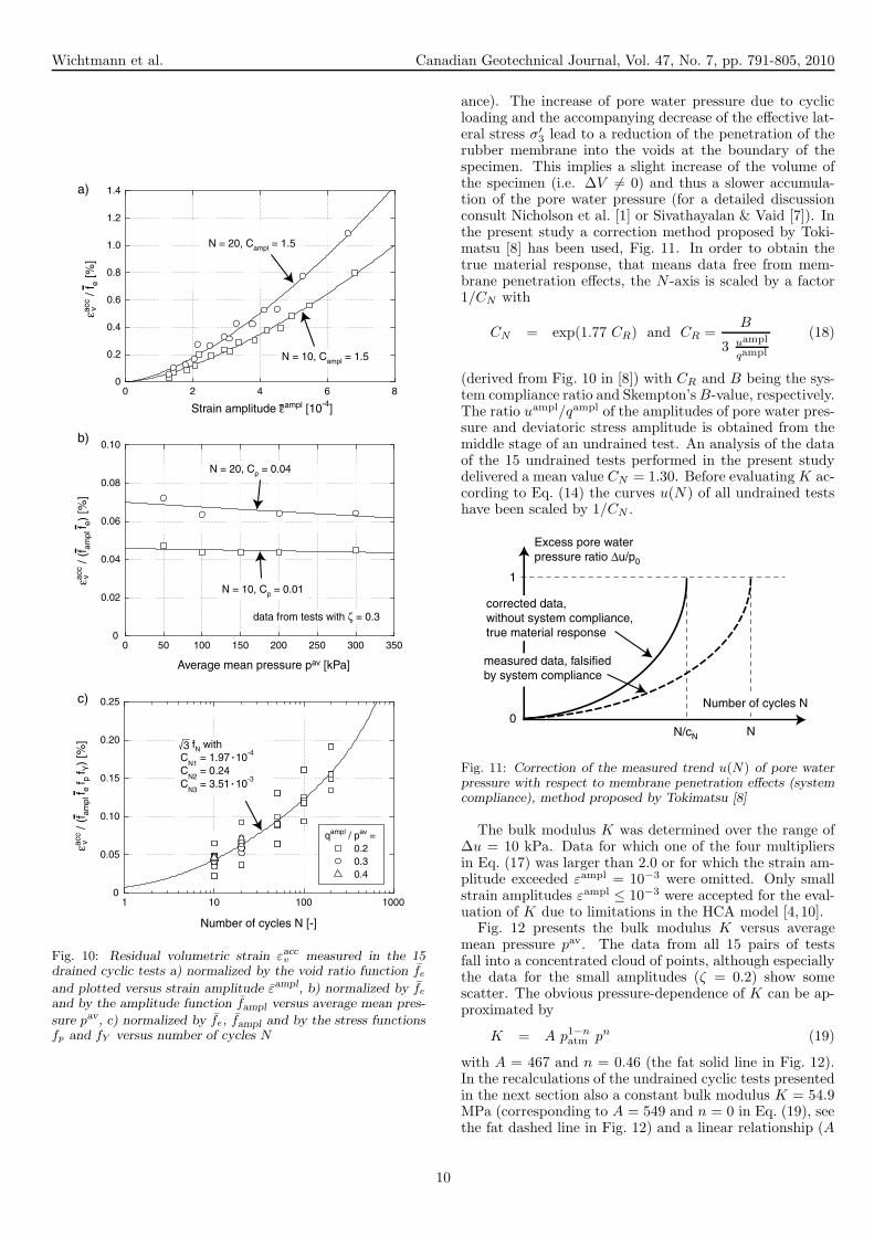
Wichtmann et al. Canadian Geotechnical Journal, Vol. 47, No. 7, pp. 791-805, 2010
0 50 100 150 200 250 300 3500
0.02
0.04
0.06
0.08
0.10
Average mean pressure pav [kPa]
0 2 4 6 80
0.2
0.4
0.6
0.8
1.0
1.2
1.4
Strain amplitude εampl [10-4]
1 10 100 10000
0.05
0.10
0.15
0.20
0.25
Number of cycles N [-]
εacc
/ fe
[%]
εacc
/ (f a
mpl
f e)
[%]
εacc
/ (f a
mpl
f e f p
f Y)
[%]
N = 10, Campl = 1.5
N = 20, Campl = 1.5
N = 20, Cp = 0.04
N = 10, Cp = 0.01
qampl / pav = 0.2 0.3 0.4
fN with C
N1 = 1.97 10-4
CN2
= 0.24 C
N3 = 3.51 10-3
vv
v
data from tests with ζ = 0.3
a)
b)
c)
3
Fig. 10: Residual volumetric strain εaccv measured in the 15
drained cyclic tests a) normalized by the void ratio function fe
and plotted versus strain amplitude εampl, b) normalized by fe
and by the amplitude function fampl versus average mean pres-
sure pav, c) normalized by fe, fampl and by the stress functionsfp and fY versus number of cycles N
ance). The increase of pore water pressure due to cyclicloading and the accompanying decrease of the effective lat-eral stress σ′
3 lead to a reduction of the penetration of therubber membrane into the voids at the boundary of thespecimen. This implies a slight increase of the volume ofthe specimen (i.e. ∆V 6= 0) and thus a slower accumula-tion of the pore water pressure (for a detailed discussionconsult Nicholson et al. [1] or Sivathayalan & Vaid [7]). Inthe present study a correction method proposed by Toki-matsu [8] has been used, Fig. 11. In order to obtain thetrue material response, that means data free from mem-brane penetration effects, the N -axis is scaled by a factor1/CN with
CN = exp(1.77 CR) and CR =B
3 uampl
qampl
(18)
(derived from Fig. 10 in [8]) with CR and B being the sys-tem compliance ratio and Skempton’s B-value, respectively.The ratio uampl/qampl of the amplitudes of pore water pres-sure and deviatoric stress amplitude is obtained from themiddle stage of an undrained test. An analysis of the dataof the 15 undrained tests performed in the present studydelivered a mean value CN = 1.30. Before evaluating K ac-cording to Eq. (14) the curves u(N) of all undrained testshave been scaled by 1/CN .
NN/cN
Excess pore water pressure ratio ∆u/p0
1
0Number of cycles N
corrected data, without system compliance, true material response
measured data, falsified by system compliance
Fig. 11: Correction of the measured trend u(N) of pore waterpressure with respect to membrane penetration effects (systemcompliance), method proposed by Tokimatsu [8]
The bulk modulus K was determined over the range of∆u = 10 kPa. Data for which one of the four multipliersin Eq. (17) was larger than 2.0 or for which the strain am-plitude exceeded εampl = 10−3 were omitted. Only smallstrain amplitudes εampl ≤ 10−3 were accepted for the eval-uation of K due to limitations in the HCA model [4, 10].
Fig. 12 presents the bulk modulus K versus averagemean pressure pav. The data from all 15 pairs of testsfall into a concentrated cloud of points, although especiallythe data for the small amplitudes (ζ = 0.2) show somescatter. The obvious pressure-dependence of K can be ap-proximated by
K = A p1−natm pn (19)
with A = 467 and n = 0.46 (the fat solid line in Fig. 12).In the recalculations of the undrained cyclic tests presentedin the next section also a constant bulk modulus K = 54.9MPa (corresponding to A = 549 and n = 0 in Eq. (19), seethe fat dashed line in Fig. 12) and a linear relationship (A
10
Wichtmann et al. Canadian Geotechnical Journal, Vol. 47, No. 7, pp. 791-805, 2010
= 331 and n = 1, see the fat dot-dashed line in Fig. 12)were tried out. The constant bulk modulus is the meanvalue of all data in Fig. 12.
The data for the large amplitude-pressure ratio ζ = 0.4lay at the upper boundary of the cloud of data in Fig. 12while the data for ζ = 0.2 are located at the lower bound-ary. However, this slight amplitude-dependence may beneglected for practical purpose.
The data in Figure 12 gives no evidence that K de-pends on cyclic preloading (i.e. on the number of cyclesN). Hence, a conclusion of an earlier publication has to berevised. In [16] the data from drained and undrained cyclictests has been analyzed using the constants in the third col-umn of Table 1 (i.e. the constants determined from testswith a large number of cycles) and no correction for mem-brane penetration effects was applied.
8 Numerical simulation of element tests with theHCA model
The good approximation of the experimental data from thedrained tests by the HCA model with the constants in thefourth column of Table 1 is demonstrated in the middlecolumn of diagrams in Fig. 9 where the predicted trendcurves εacc
v (N) have been added (solid lines). The initialvoid ratios and the measured curves of the strain amplitudeεampl(N) were used as an input for the recalculations. De-spite some deviations for pav = 50 kPa and for amplitude-pressure ratios of ζ = 0.2 and 0.3, the measured and thepredicted curves agree well.
The undrained cyclic tests have been recalculated us-ing the HCA model with K obtained from Eq. (19) andwith the constants given in the fourth column of Table1. The initial void ratios and the measured curves of thestrain amplitude εampl(N) were used as an input. In con-trast to the experimental data the curves u(N) predictedby the HCA model are free from membrane penetrationeffects. Therefore, for comparison purpose the N -axis hasbeen scaled by a factor 1.3 (therefore the predicted curvesstart at N = 1.3).
Three different pairs of constants A and n in Eq. (19)were tried out. The constants A = 467 and n = 0.46approximate well the pressure-dependence of the data inFig. 12. Using these constants, the trend u(N) predictedby the HCA model agrees quite well with the experimentaldata (see the middle column of diagrams in Fig. 7), excepta large deviation in case of the test with p0 = 50 kPa andζ = 0.2. The surprisingly low accumulation of pore waterpressure in the test with pav = 50 kPa and ζ = 0.2 may bedue to preloading or aging effects since an effective stressof 50 kPa was also applied during the specimen prepara-tion procedure. While these effects may not influence theaccumulation at larger amplitudes and pressures, they mayhave reduced the rates u for the small amplitude-pressureratio ζ = 0.2.
For FE calculations a constant bulk modulus (A = 549and n = 0) or a linear relationship (A = 331 and n = 1)would be advantageous for numerical reasons. The constantvalue overestimates the bulk modulus at small pressuresand underestimates it at large pressures (Fig. 12). For alinear approximation of K(p) it is the other way around.Consequently, the dashed curves u(N) in Fig. 7 reveal thata constant bulk modulus overestimates the accumulation of
pore water pressure in the tests with small initial pressures(p0 = 50 and 100 kPa) while the rate u is underestimatedin the tests with a large initial pressure (p0 = 300 kPa).The usage of a linear relationship for K(p) results in anunderestimation of the pore water pressure accumulation inthe tests with initial pressures p0 = 50 and 100 kPa whilethe prediction is still acceptable for p0 = 300 kPa (dot-dashed curves in Fig. 7). For intermediate initial pressures(p0 = 150 and 200 kPa) all three sets of constants for A andn deliver similar bulk moduli and thus approximate well themeasured data. However, based on the predicted curvesu(N) in Fig. 7 it can be stated that for FE calculationsinvolving poor drainage conditions the usage of a constantor a linear function for K(p) seems to be over-simplified.
It can be concluded that the HCA model with a single setof constants (fourth column of Table 1) in combination withthe pressure-dependent bulk modulus derived in the presentstudy (Eq. (19) with A = 467 and n = 0.46) describes wellboth, the accumulation of pore water pressure in undrainedcyclic tests and the accumulation of volumetric strain indrained cyclic tests.
9 Simplified determination of K
Judging by the presented test results a proper determi-nation of K(p) requires at least two pairs of drained andundrained cyclic tests with different initial effective meanpressures (e.g. p0 = 100 and 300 kPa). The tests couldbe performed for example with an intermediate amplitude-pressure ratio of ζ = 0.3. For coarse-grained sands mem-brane penetration effects may become considerable (accord-ing to Nicholson et al. [1] they increase over-proportionallywith the grain size d20) and the procedure discussed abovemay not be sufficiently accurate. Alternatively to this cali-bration a simplified procedure has been studied. The mod-ulus K is estimated from oedometric or resonant columntest data.
Two tests with oedometric compression (specimen di-ameter d = 10 cm, height h = 3.5 cm) were performed ondry sand. The initial relative density ID0 was 0.63 in bothtests. The maximum axial stress was σ1 = 2 MPa. A singleun- and reloading cycle was performed. The evolution ofvoid ratio e in the tests is given in Figure 13. The bulkmodulus was estimated from the constrained elastic mod-ulus M = ∆σ1/∆ε1 using the relationship K = 1+ν
3(1−ν)M .
Curves K(p) for two different values of Poisson’s ratio (ν= 0.2 and ν = 0.25, respectively) have been added to Fig-ure 12 (narrow dashed curves). They represent mean val-ues of the two performed tests. In order to calculate p,the lateral stress in the oedometric tests was estimatedfrom σ3 = K0σ1 using Jaky’s formula K0 = 1 − sin ϕc
with the critical friction angle ϕc = 31.2◦ which was deter-mined from a pluviated cone of sand. Figure 12 reveals thatthe bulk modulus from the comparison of the drained andundrained cyclic tests agrees quite well with the bulk modu-lus obtained from the oedometric compression tests duringun- and reloading. This seems to be quite reasonable sincean increase of the pore water pressure and the accompa-nying decrease of the effective mean pressure correspondsto an elastic unloading. Hence, the approach of Sawicki [6]could be confirmed. Therefore, a simplified procedure us-ing merely the un- and reloading curve in an oedometriccompression test provides a sufficiently exact estimate of
11
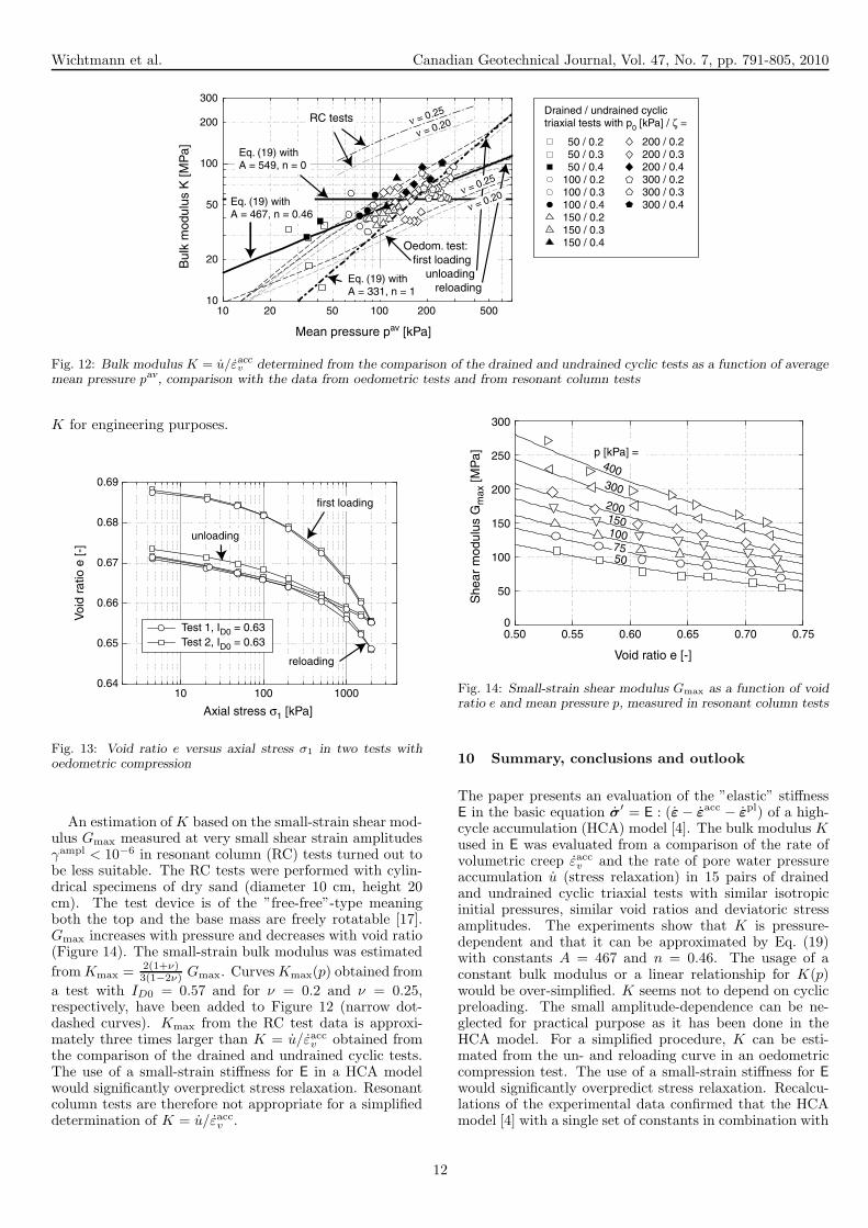
Wichtmann et al. Canadian Geotechnical Journal, Vol. 47, No. 7, pp. 791-805, 2010
10 20 50 100 200 50010
20
50
100
200
300
50 / 0.250 / 0.350 / 0.4
100 / 0.2100 / 0.3100 / 0.4150 / 0.2150 / 0.3150 / 0.4
200 / 0.2200 / 0.3200 / 0.4300 / 0.2300 / 0.3300 / 0.4
Bul
k m
odul
us K
[MP
a]
Mean pressure pav [kPa]
Drained / undrained cyclic triaxial tests with p0 [kPa] / ζ =ν = 0.25
ν = 0.20RC tests
Eq. (19) with A = 467, n = 0.46
Eq. (19) with A = 549, n = 0
Oedom. test: first loading unloading reloading
ν = 0.25
ν = 0.20
Eq. (19) with A = 331, n = 1
Fig. 12: Bulk modulus K = u/εaccv determined from the comparison of the drained and undrained cyclic tests as a function of average
mean pressure pav, comparison with the data from oedometric tests and from resonant column tests
K for engineering purposes.
10 100 10000.64
0.65
0.66
0.67
0.68
0.69
Test 1, ID0 = 0.63
Test 2, ID0 = 0.63
Voi
d ra
tio e
[-]
Axial stress σ1 [kPa]
first loading
unloading
reloading
Fig. 13: Void ratio e versus axial stress σ1 in two tests withoedometric compression
An estimation of K based on the small-strain shear mod-ulus Gmax measured at very small shear strain amplitudesγampl < 10−6 in resonant column (RC) tests turned out tobe less suitable. The RC tests were performed with cylin-drical specimens of dry sand (diameter 10 cm, height 20cm). The test device is of the ”free-free”-type meaningboth the top and the base mass are freely rotatable [17].Gmax increases with pressure and decreases with void ratio(Figure 14). The small-strain bulk modulus was estimated
from Kmax = 2(1+ν)3(1−2ν) Gmax. Curves Kmax(p) obtained from
a test with ID0 = 0.57 and for ν = 0.2 and ν = 0.25,respectively, have been added to Figure 12 (narrow dot-dashed curves). Kmax from the RC test data is approxi-mately three times larger than K = u/εacc
v obtained fromthe comparison of the drained and undrained cyclic tests.The use of a small-strain stiffness for E in a HCA modelwould significantly overpredict stress relaxation. Resonantcolumn tests are therefore not appropriate for a simplifieddetermination of K = u/εacc
v .
0.50 0.55 0.60 0.65 0.70 0.750
50
100
150
200
250
300
She
ar m
odul
us G
max
[MP
a]
Void ratio e [-]
p [kPa] =400
200
100
300
150
7550
Fig. 14: Small-strain shear modulus Gmax as a function of voidratio e and mean pressure p, measured in resonant column tests
10 Summary, conclusions and outlook
The paper presents an evaluation of the ”elastic” stiffnessE in the basic equation σ
′ = E : (ε − εacc − ε
pl) of a high-cycle accumulation (HCA) model [4]. The bulk modulus Kused in E was evaluated from a comparison of the rate ofvolumetric creep εacc
v and the rate of pore water pressureaccumulation u (stress relaxation) in 15 pairs of drainedand undrained cyclic triaxial tests with similar isotropicinitial pressures, similar void ratios and deviatoric stressamplitudes. The experiments show that K is pressure-dependent and that it can be approximated by Eq. (19)with constants A = 467 and n = 0.46. The usage of aconstant bulk modulus or a linear relationship for K(p)would be over-simplified. K seems not to depend on cyclicpreloading. The small amplitude-dependence can be ne-glected for practical purpose as it has been done in theHCA model. For a simplified procedure, K can be esti-mated from the un- and reloading curve in an oedometriccompression test. The use of a small-strain stiffness for E
would significantly overpredict stress relaxation. Recalcu-lations of the experimental data confirmed that the HCAmodel [4] with a single set of constants in combination with
12
Wichtmann et al. Canadian Geotechnical Journal, Vol. 47, No. 7, pp. 791-805, 2010
the bulk modulus K given by Eq. (19) describes well both,the accumulation of pore water pressure in undrained cyclictests and the accumulation of volumetric strain in drainedcyclic tests.
In future, the void-ratio dependence of K will be stud-ied and an appropriate extension of Eq. (19) will be pro-posed if necessary. The minor amplitude-dependence ob-served in the experiments needs further inspection. Pois-son’s ratio ν can be evaluated from displacement-controlledundrained cyclic triaxial tests with anisotropic initialstresses (Fig. 2b). At present it is recommended to choosePoisson’s ratio in the range 0.2 ≤ ν ≤ 0.3 for calculationswith the HCA model.
Acknowledgements
The experimental work was done as a part of the projectA8 ”Influence of the fabric change in soil on the lifetimeof structures”, supported by the German Research Coun-cil (DFG) within the Collaborate Research Centre SFB398 ”Lifetime oriented design concepts” at Ruhr-UniversityBochum. The authors are indepted to DFG for this finan-cial support.
References
[1] P.G. Nicholson, R.B. Seed, and H.A. Anwar. Elim-ination of membrane compliance in undrained triax-ial testing. I. Measurement and evaluation. CanadianGeotechnical Journal, 30:727–738, 1993.
[2] A. Niemunis. Extended hypoplastic models forsoils. Habilitation, Veroffentlichungen des Insti-tutes fur Grundbau und Bodenmechanik, Ruhr-Universitat Bochum, Heft Nr. 34, 2003. available fromwww.pg.gda.pl/∼aniem/an-liter.html.
[3] A. Niemunis and I. Herle. Hypoplastic model for co-hesionless soils with elastic strain range. Mechanics ofCohesive-Frictional Materials, 2:279–299, 1997.
[4] A. Niemunis, T. Wichtmann, and T. Triantafyllidis. Ahigh-cycle accumulation model for sand. Computersand Geotechnics, 32(4):245–263, 2005.
[5] A. Niemunis, T. Wichtmann, and Th. Triantafyllidis.On the definition of the fatigue loading for sand. InInternational Workshop on Constitutive Modelling -Development, Implementation, Evaluation, and Appli-cation, 12-13 January 2007, Hong Kong, 2007.
[6] A. Sawicki. Modelling earthquake-induced phenomenain the Izmit Bay coastal area. In Th. Triantafyllidis,editor, Cyclic Behaviour of Soils and LiquefactionPhenomena, Proc. of CBS04, Bochum, March/April2004, pages 431–440. Balkema, 2004.
[7] S. Sivathayalan and Y.P. Vaid. Truly undrained re-sponse of granular soils with no membrane-penetrationeffects. Canadian Geotechnical Journal, 35(5):730–739, 1998.
[8] K. Tokimatsu. System compliance correction frompore pressure response in undrained triaxial tests.Soils and Foundations, 30(2):14–22, 1990.
[9] P.-A. von Wolffersdorff. A hypoplastic relation forgranular materials with a predefined limit state sur-face. Mechanics of Cohesive-Frictional Materials,1:251–271, 1996.
[10] T. Wichtmann. Explicit accumulation model fornon-cohesive soils under cyclic loading. PhD the-sis, Publications of the Institute of Soil Mechan-ics and Foundation Engineering, Ruhr-UniversityBochum, Issue No. 38, available from www.rz.uni-karlsruhe.de/∼gn97/, 2005.
[11] T. Wichtmann, A. Niemunis, and T. Triantafyllidis.Strain accumulation in sand due to cyclic loading:drained triaxial tests. Soil Dynamics and EarthquakeEngineering, 25(12):967–979, 2005.
[12] T. Wichtmann, A. Niemunis, and T. Triantafyllidis.On the influence of the polarization and the shapeof the strain loop on strain accumulation in sand un-der high-cyclic loading. Soil Dynamics and EarthquakeEngineering, 27(1):14–28, 2007.
[13] T. Wichtmann, A. Niemunis, and T. Triantafyllidis.Strain accumulation in sand due to cyclic loading:drained cyclic tests with triaxial extension. SoilDynamics and Earthquake Engineering, 27(1):42–48,2007.
[14] T. Wichtmann, A. Niemunis, and T. Triantafyllidis.Validation and calibration of a high-cycle accumula-tion model based on cyclic triaxial tests on eight sands.Soils and Foundations, 49(5):711–728, 2009.
[15] T. Wichtmann, A. Niemunis, T. Triantafyllidis, andM. Poblete. Correlation of cyclic preloading with theliquefaction resistance. Soil Dynamics and EarthquakeEngineering, 25(12):923–932, 2005.
[16] T. Wichtmann, A. Niemunis, and Th. Triantafyllidis.Recent advances in constitutive modelling of com-paction of granular materials under cyclic loading. InN. Bazeos, D.C. Karabalis, D. Polyzos, D.E. Beskos,and J.T. Katsikadelis, editors, Proc. of 8th HSTAMInternational Congress on Mechanics, Patras, Greece12 14 July, volume 1, pages 121–136. Hellenic Societyfor Theoretical and Applied Mechanics, Athens, 2007.
[17] T. Wichtmann and T. Triantafyllidis. On the in-fluence of the grain size distribution curve of quartzsand on the small strain shear modulus Gmax. Jour-nal of Geotechnical and Geoenvironmental Engineer-ing, ASCE, 135(10):1404–1418, 2009.
List of symbols
B Skempton’s B-valueCN Membrane penetration correction factorCR System compliance ratioδij Kronecker’s symbole Void ratioε1 Axial strainε3 Lateral strainεv Volumetric strainεq Deviatoric strainεampl Strain amplitudeεacc Residual (accumulated) strain
13
Wichtmann et al. Canadian Geotechnical Journal, Vol. 47, No. 7, pp. 791-805, 2010
εacc Intensity of strain accumulationε Strain tensorε Trend of strainεacc Rate of strain accumulation
εpl Plastic strain rate
E Young’s modulusE Elastic stiffness tensorϕc Critical friction anglefampl Amplitude function (HCA model)fc Correction factorfe Void ratio function (HCA model)fN Function for cyclic preloading (HCA model)fp Pressure function (HCA model)fY Stress ratio function (HCA model)fπ Function for polarization changes (HCA model)F Correction factor for Mγampl Shear strain amplitudegA Historiotropic variable (HCA model)G Shear modulusGmax Small strain shear modulusη Stress ratioηav Average stress ratioID Relative densityK Bulk modulusK0 Earth pressure coefficient at restλ Lame constantµ Lame constantmv Volumetric component of mmq Deviatoric component of mM Constrained elastic modulusM Critical stress ratioMc Critical stress ratio for triax. compr.Me Critical stress ratio for triax. ext.m Direction of strain accumulationν Poisson’s ratioN Number of cyclesp Effective mean pressurepav Average effective mean pressureq Deviatoric stressqampl Deviatoric stress amplitudeσ1 Total axial stressσ′
1 Effective axial stressσ3 Total lateral stressσ′
3 Effective lateral stressσ
′ Effective stress tensorσ
′ Trend of effective stressu Pore water pressureY Normalized stress ratioζ Amplitude-pressure ratio1 Second-order identity tensorI Fourth-order identity tensor
14