Can Structural Change Explain the Decrease in Returns

to Technical Analysis?

By

Willis V. Kidd and B. Wade Brorsen

Suggested citation format:

Kidd, W. V., and B. W. Brorsen. 2002. “Can Structural Change Explain the Decrease in Returns to Technical Analysis?” Proceedings of the NCCC-134 Conference on Applied Commodity Price Analysis, Forecasting, and Market Risk Management. St. Louis, MO. [http://www.farmdoc.uiuc.edu/nccc134].

Can Structural Change Explain

the Decrease in Returns to Technical Analysis?

Willis V. Kidd

and

B. Wade Brorsen*

Paper presented at the NCR-134 Conference on Applied Commodity PriceAnalysis, Forecasting, and Market Risk Management

St. Louis, Missouri, April 22-23, 2002

Copyright 2002 by Willis V. Kidd and B. Wade Brorsen. All rights reserved.Readers may make verbatim copies of this document for non-commercial purposes by

any means, provided that this copyright notice appears on all such copies.

*Kidd is a graduate research assistant, and Brorsen is a regents professorand Jean & Patsy Neustadt Chair (brorsen@okstate.edu),

Department of Agricultural Economics, Oklahoma State University

1

Can Structural Change Explain Changes in Returns to Technical Analysis?

Practitioners Abstract:

Returns to managed futures funds and Commodity Trading Advisors (CTAs) havedecreased dramatically during the last several years. Since these funds overwhelminglyuse technical analysis, this research examines futures prices to determine if there isevidence of a structural change in futures price movements that could explain thereduction in fund returns. Bootstrap tests are used to test significance of a change instatistics related to daily returns, close-to-open changes, breakaway gaps, and serialcorrelation. Results indicate that several statistics have changed across a broad range ofcommodities indicating futures price fluctuations have changed. The lower pricevolatility, decreased price reaction time, and decreased serial correlation may partlyexplain the lower returns from technical analysis.

Keywords: Structural Change, Bootstrap, Managed Futures, Commodity TradingAdvisor, Technical Analysis

Introduction

The managed futures industry has been a quickly growing segment of the financial world.In recent years however, futures fund returns have decreased and the value of assetsinvested in managed futures has decreased along with returns. Figure 1 shows theBarclay Commodity Trading Advisor Index versus time and shows a steady trend ofdecreasing returns during the past twenty years. The causes of this decrease in fundperformance are not fully known. Two possible explanations for the decrease are adecrease in market volatility (and therefore profit opportunities) and price distortioncaused by the growth of the industry. Certainly there must have been changes in thedistribution of futures prices in order for returns to have decreased so dramatically1. Thisnaturally leads to the research question, “What structural changes have occurred infutures price movements?” Knowing the way futures price distributions have changedwill help explain why futures fund returns have decreased.

Most financial participants are at least superficially interested in the return characteristicsof managed futures funds and Commodity Trading Advisors. Technically tradedmanaged futures funds rely almost exclusively on past prices to generate buy and sellsignals. Accordingly the returns to these funds depend on weak-form inefficiency of themarkets. Therefore the return attributes of managed futures funds are of high interest notonly to investors but also to regulators, investment advisors, and policy makers.Technical analysis has been advocated as a way for farmers to make buying and sellingdecisions (e.g. Purcell; Franzmann and Sronce). Many of the farmer advisory servicestracked by Irwin et. al. base their recommendations partly on technical analysis. The

1 Indeed there have been many charges that trading by the funds has distorted prices, including cattle pricesin 2002. But the evidence in support of these charges is still inconclusive (Brorsen and Irwin; Holt andIrwin; Commodity Futures Trading Commission).

2

dramatic decrease in technical profitability indicates that futures markets have becomemore efficient. Research is needed to determine the ways in which the market haschanged, thereby allowing technical traders to adjust trading systems to account for thesechanges.

Most previous studies of returns to managed futures funds focus on the predictability ofreturns (e.g. Schwager; Brorsen and Townsend), factors that increase returns (e.g. Irwinand Brorsen 1987), and if an increase in the trading volume of managed futures fundsdecreases returns (e.g. Brorsen and Irwin 1987; Holt and Irwin). Some authors haveexamined the profitability of technical trading (e.g. Lukac and Brorsen 1990; Brock,Lakonishok, and LeBaron, Osler and Chang), and Boyd and Brorsen used simulatedtechnical trading profits to see which price statistics are correlated with technical returns,but no authors have compared actual trading profits to price statistics. Furthermore,many authors have examined the distribution (e.g. Mandelbrot; Gordon) and dependence(e.g. Gordon; Mann; Trevino and Martell) of futures price changes. The few studies thathave evaluated a possible change in price distributions and dependence are limited instatistical techniques and commodities tested. Using cash prices, Brorsen found thatautocorrelations of the Standard and Poor 500 stock index had decreased and the varianceof returns had increased over the period 1962 to 1986. Although not backed by formalsignificance tests, Hudson, Leuthold, and Sarassoro suggest that price changes havebecome more normal over time. No research has comprehensively studied a change indaily return characteristics. This research will analyze futures prices directly to test thehypothesis that a structural change in price fluctuations has occurred that may haveaffected the profitability of managed futures and technical analysis. This will beaccomplished using bootstrap resampling techniques to test for evidence of a structuralchange in the dependence and distribution of futures prices.

Economic Theory

Managed futures funds overwhelmingly use technical trading systems to formulate buyand sell decisions (Irwin and Brorsen; Billingsley and Chance). Therefore the ability togenerate positive net returns depends on the manner in which prices move. Anydevelopment in the futures industry that can change the way prices fluctuate could havechanged the returns to technical analysis. If a structural change in price fluctuations hasoccurred, technical trading systems developed prior to the change may be obsolete, orchanges may indicate that the need for technical trading to move the market toequilibrium has decreased.

The most popular forms of technical analysis are trend-following methods (e.g.Billingsley and Chance; Kaufmann; Commodity Futures Trading Commission). Whilesome economists have placed technical analysis in the same category as astrology, thereare sound theoretical explanations for the profitability of trend-following systems.Disequilibrium models such as those developed by Beja and Goldman and Grossman andStiglitz are based on the assumption that prices do not instantaneously fully react to aninformation shock. Fundamental traders start moving the price toward equilibrium, butare unable to fully move the market due to risk aversion, capital constraints, or position

3

limits. The result is price trends that technical analysts can detect and trade. Thetrending periods would be reflected in positive autocorrelation. Thus any reduction in theautocorrelation of futures prices will decrease the profitability of trend-followingsystems. Empirical research, however, has only been able to detect a small amount ofautocorrelation beyond what would be expected in an uncorrelated series (Irwin andUhrig). The theoretical arguments for trend-following systems are based on a delayedmovement toward equilibrium after new information enters the marketplace. Theincreased speed of news dissemination and market transactions and the increased use oftrend-following systems likely have decreased the duration of market trends.

A structural change in futures markets could be caused by many developments.Fundamental changes in markets have the possibility of modifying the way and speed inwhich traders react. A decrease in the cost of information, increase in the speed offinancial transactions, decrease in computing cost, and an increase in the relative use oftechnical analysis, all have the potential to change the way prices fluctuate by increasingthe reaction to new information and driving the market to equilibrium faster. Thesedevelopments will have decreased the cost of using technical analysis and therefore mayhave decreased its profitability. In addition to these developments directly related to thefutures industry, there are many economy wide changes that may have affected futuresprices. Freer trade, better economic predictions, and fewer major shocks to the economyall may have lowered price volatility and therefore lowered the need for technicalspeculators to move the markets to equilibrium. Previous research by Boyd and Brorsensupports this theory as they found a strong relationship between market volatility andtechnical trading profits.

Developments in the past several years may have allowed markets to react faster to newinformation. If new information becomes available overnight, the change in pricesbetween the close and open would be large. If price movements occur overnight thenfunds will either miss trading opportunities or will have to trade in the overnight marketsthat have higher liquidity costs. It is expected that advancements in markets such asincreased news and transaction speed have caused the variance and kurtosis of close-to-open gaps to increase; however, the expected increase in the variance of gaps may beoffset by a decrease in overall market volatility.

These possible changes in prices leads to the first hypothesis of structural change in dailyfutures prices:

1) There is a decreased demand for technical trading due to market developmentsand macroeconomic change. These changes will be shown through reduced pricevolatility and decreased market reaction time.

Another possible explanation for the reduced technical trading profitability is that largeincrease in the managed futures industry has distorted prices. Lukac, Brorsen, and Irwinfound that different simulated technical trading systems signaled trades on the same day asignificant number of days, which may allow for price distortion. In a recent CommodityFutures Trading Commission Report (page 7), the market surveillance staff reported:

4

Over many years of observing the activity of commodity funds, the Surveillancestaff has observed that, although a large number of funds may hold positions in amarket, most of them do not trade on any given day. When funds do trade,however, they tend to trade in the same directions. Since many funds usetechnical, trend-following, trading systems, it is not clear whether fund activitycontributes to the magnitude or direction of the price change or whether they arereacting to the price change.

Empirical research is inconsistent as to whether an increase in the size of managedfutures increases price volatility (e.g. Brorsen and Irwin; Holt and Irwin; Irwin andBrorsen). Increased technical trading should speed price adjustments (i.e. reduceinefficiency), but it would also increase the variance and kurtosis of price movements(Brorsen, Oellermann, and Farris).

The possibility of price distortion leads to the second hypothesis of structural change indaily futures prices:

2) The increase in the size of the managed futures industry has increased pricevolatility, increased price kurtosis, and decreased autocorrelations, by eitherincreasing market efficiency or price distortion through similarity of trading.

These two hypotheses represent two possible ways that a change in daily futures pricebehavior may be reflected in reduced technical profitability.

Data

Daily futures prices from seventeen commodities were used to test hypotheses regardinga structural change in daily price movements. A diverse set of commodities was selectedrepresenting four sectors: agricultural, financial, foreign exchange rates, and preciousmetals. The data were collected from the Bridge/CRB commodity database. The tests ofstructural change separate the data into two distinct time periods. Time period one beginson January 1, 1975 or the first date on which data were available, and ends on December31, 1990. Time period two begins on January 1, 1991 and ends on December 31, 2001.The split date was selected to coincide with the drop in technical trading returns as shownin Figure 1.

In order to analyze the contracts typically traded by managed futures funds, a continuousseries of prices was constructed utilizing a contract until thirty trading days prior to theexpiration of a contract, then the price series uses the next subsequent contract month.The changes in variables were calculated before splicing the data so that no outliers arecreated when contracts are rolled over.

Three market related variables were analyzed: daily returns, close-to-open price changes,and daily trading gaps. Percent daily returns are defined as:

5

(1) )ln(ln*100 1−−= ttt ssr

where rt is the daily return for day t, and st is the futures settlement price for day t. Close-to-open price changes are the gaps between the settlement price of a futures contract andthe opening price on the following day. Therefore,

(2) 1lnln −−= ttt soc

where ct is the logarithmic close-to-open change, ot is the opening price on day t, andst-1 is the previous day’s settlement price. The final statistic, breakaway trading gaps, is

(3)

�

�

�

≥−≤−

= −−

−−

otherwise,"missing"if,lnlnif,lnln

11

11

tttt

tttt

t hlhllhlh

g

where gt is the trading gap, ht is the highest price attained on day t, and lt is the lowestprice attained on day t.

Statistics Tested

Daily Return Statistics. More statistics are calculated for the daily returns than for othervariables. Both short-term and long-term statistics are generated. There are threedistributional statistics that are calculated for daily returns: sample variance, skewness,and kurtosis.

The p-day logarithmic return was calculated by summing daily returns. Long-run returnsare calculated for lengths of 5 (weekly), 10 (biweekly), and 20 (approximately monthly)days. The long-run returns are overlapping in order to allow for greater power ofbootstrap statistical tests (Harri and Brorsen). The variance of weekly, biweekly, andmonthly returns is calculated and analyzed for changes in long-run volatility.

The multi-day returns also allow comparing short-run and long-run effects. In order tocompare daily returns to returns of longer time horizons, ratios of daily variance to 5, 10,and 20 day variances were calculated. Variance ratios have been used in marketefficiency tests (Poterba and Summers; Lo and Mackinlay). With independent andidentically distributed normal random variables, the variance of p-day returns is p timesthat of daily returns. Positive autocorrelation would cause variance ratios to be less than1/p. The variance ratios of Lo and MacKinlay also use overlapping data.

Daily Breakaway Gap and Close-to-Open Change Statistics. The same statistics will becalculated for both gaps and close-to-open changes. These statistics are intended tosummarize the size and distribution of these variables. Four sample statistics will becalculated for each variable: mean, variance, relative skewness, and relative kurtosis.

6

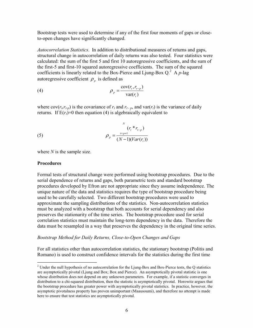
Bootstrap tests were used to determine if any of the first four moments of gaps or close-to-open changes have significantly changed.

Autocorrelation Statistics. In addition to distributional measures of returns and gaps,structural change in autocorrelation of daily returns was also tested. Four statistics werecalculated: the sum of the first 5 and first 10 autoregressive coefficients, and the sum ofthe first-5 and first-10 squared autoregressive coefficients. The sum of the squaredcoefficients is linearly related to the Box-Pierce and Ljung-Box Q.2 A p-lagautoregressive coefficient pρ is defined as

(4))var(

),cov(

t

pttp r

rr −=ρ

where cov(rt,rt-p) is the covariance of rt and rt - p, and var(rt) is the variance of dailyreturns. If E(rt)=0 then equation (4) is algebraically equivalent to

(5)))()(1(

)*(1

t

N

ptptt

p rVarN

rr

−= +=

−

ρ

where N is the sample size.

Procedures

Formal tests of structural change were performed using bootstrap procedures. Due to theserial dependence of returns and gaps, both parametric tests and standard bootstrapprocedures developed by Efron are not appropriate since they assume independence. Theunique nature of the data and statistics requires the type of bootstrap procedure beingused to be carefully selected. Two different bootstrap procedures were used toapproximate the sampling distributions of the statistics. Non-autocorrelation statisticsmust be analyzed with a bootstrap that both accounts for serial dependency and alsopreserves the stationarity of the time series. The bootstrap procedure used for serialcorrelation statistics must maintain the long-term dependency in the data. Therefore thedata must be resampled in a way that preserves the dependency in the original time series.

Bootstrap Method for Daily Returns, Close-to-Open Changes and Gaps

For all statistics other than autocorrelation statistics, the stationary bootstrap (Politis andRomano) is used to construct confidence intervals for the statistics during the first time 2 Under the null hypothesis of no autocorrelation for the Ljung-Box and Box-Pierce tests, the Q statisticsare asymptotically pivotal (Ljung and Box; Box and Pierce). An asymptotically pivotal statistic is onewhose distribution does not depend on any unknown parameters. For example, if a statistic converges indistribution to a chi-squared distribution, then the statistic is asymptotically pivotal. Horowitz argues thatthe bootstrap procedure has greater power with asymptotically pivotal statistics. In practice, however, theasymptotic pivotalness property has proven unimportant (Maausoumi), and therefore no attempt is madehere to ensure that test statistics are asymptotically pivotal.

7

period. This type of bootstrap is applicable to weakly dependent stationary time seriesand has been used in financial studies such as White, Sullivan, and Timmerman, andWhite.

The formation of the pseudo time series involves many steps. Let N1 be the sample sizeof the first time period and N2 be the sample size of the second time period. First thelength of the block, l, is determined. This random length varies according to a geometric(.10) variable. Next the starting observation, s, is chosen by randomly selecting a numberaccording to a discrete uniform distribution. The starting block is generated by x1* =[xS,xS+1,…xS+l-1]. This process is repeated by selecting a new l and s to generate x2*. Thisprocess is continued and the vector X* is generated by concatenating the xi* vectors untilthe pseudo series is greater in length than N1. The generated series is then truncated suchthat the number of observations in X* equals N1, the number of elements in the first timeperiod. This process is repeated to form another pseudo-series Y*, which is a 1 x N2vector generated from stochastic length blocks of data from the first time period.

Once the pseudo time series sample is generated, the statistics of interest are calculatedon X* and Y*. For a test of a change in the mean, the difference in the mean of theelements of X* and Y* is found:

(6)==

−=Θ21

12111

11ˆN

ii

N

ii Y

NX

N

Following Good, a test in the change of the variance is performed by calculating the ratioof the variance of X* to the variance of Y*

(7)

=

=

−−

−−=Θ

2

1

1

2

2

1

2

12

)(1

1

)(1

1

ˆN

ii

N

ii

YYN

XXN

Equation (7) is used for daily, 5-day, 10-day, and 20-day returns. Tests of a change inrelative skewness and relative kurtosis use the difference in the sample relative skewnessand relative kurtosis in X* and Y*. In contrast Dufour and Farhat use the absolute valueof the change in skewness and relative kurtosis. The statistics used are thus:

(8) 31

3

22

23

1

3

11

13

21

)(

)2)(1(

)(

)2)(1(ˆ

y

N

ii

x

N

ii

s

YY

NNN

s

XX

NNN ==

−

−−−

−

−−=Θ

and

8

(9)�

����

�

�

−−−−

−

−−−+

−

�����

����

�

�

−−−

−−

−−−+

=Θ

=

=

)3)(2()1(3

)(

)3)(2)(1()1(

)3)(2()1(3

)(

)3)(2)(1()1(ˆ

22

24

1

4

222

22

11

21

41

4

111

114

1

1

NNN

s

YY

NNNNN

NNN

s

XX

NNNNN

y

N

ii

x

N

ii

where sx and sy are the sample standard deviations of X* and Y*, respectively.

The process is repeated until 1,000 new pseudo-series have been generated and the( )4,3,2,1ˆ =Θ mm statistics calculated. The actual change in the statistic, mΘ , is then

calculated. mΘ is the value of Equations (6) to (9) when the actual data from time periodone is the vector X and the actual data from time period two is the vector Y. The nullhypothesis of no change (i.e. mΘ =0) is rejected if mΘ is less than the α /2 percentile of

mΘ̂ or greater than the 1-α /2 percentiles of mΘ̂ . The levels of α selected for this studyare .05 and .10.

Bootstrap Methods for Daily Autocorrelations

Any bootstrap autocorrelation test must maintain the dependence between observations.The block bootstrap methods maintain dependence asymptotically as the size of the blockincreases to infinity (Horowitz). However, in finite samples, block bootstrap methodsalone produce autocovariance estimates that are biased toward zero. In order to fullymaintain the dependence, a new type of bootstrap procedure was developed.

Let N2 be the sample size of the second sub-period, and let p={5,10} be the length ofautoregressive lag tested. Then form C to be a (N1 – p) x (p + 1) matrix comprised of rowvectors ct where the jth element of ct is the return for day t – j + 1 from the firstsubperiod, such that ct=[rt, rt-1,…,rt-j+1,…, rt-p] for all t>p. Bootstrap confidence intervalswere formed by resampling blocks of row vectors (with replacement) from the matrix Cto form a N1 x p+1 matrix C* and a N2 x p + 1 matrix D*. The number of vectors in ablock is a geometric (.10) random variable. Therefore, C* and D* are similar to thepseudo-time series generated by the stationary bootstrap used for returns and gaps.Equation (5) can then be rewritten as

(10))var(

)*(

1,

1,1,

,i

pT

ikii

p τ

ττρ τ

−

== for },{ dc=τ

where var(τ i,1) is the variance of the first column vector of T*, (T={C,D}).

9

The statistics of interest are the differences in the autocorrelation coefficients from C*and D* adjusted by the degrees of freedom. These statistics are then calculated from thesimulated pρ ’s (10) by the equation

(11)�

���

�−=Θ

==

p

i

wdi

p

i

wci NN

1,2

1,15 **ˆ ρρ for w ={1,2}, and p={5,10}

where p is the lag and w is the power to which the autoregressive coefficient is raised.This process is repeated 1,000 times to form an empirical bootstrap distribution of the

5Θ̂ . Let D be a (N2 – p) x (p + 1) matrix formed in the same manner as C, but using datafrom the second time period. Then 5Θ is the difference in the autocorrelations from thefirst time period and the second time period (i.e. using the matrices C and D in Equations10 and 11). The null hypothesis of no change (i.e. 5Θ =0) was reject if 5Θ was less than

the α /2 percentile of 5Θ̂ or greater than the 1-α /2 percentiles of 5Θ̂ .

Since it is unlikely that a statistic will significantly change across all commodities, a ruleto determine how many commodities represent enough to conclude a change has occurredis desired. However, a rule such as this is difficult to formulate. This is due in large partto prices of many commodities being correlated with prices of other commodities.Furthermore, this dependency is not constant between commodities. Therefore any ruledevised using standard statistical methods has been ruled out as inappropriate and an adhoc rule was formulated. In order to save space in this paper and prevent reportingseveral pages of insignificant statistics, only those statistics that have changed in one halfor more of the commodities or have substantial theoretical explanations will be presentedand explained. This will allow more emphasis on statistics that have more evidence ofchange than discussing all commodity-statistic pairs that have changed.

Results

The tests of structural change are presented in Table 1 through Table 8.3 There is definiteevidence of a structural change in futures price returns, gaps, and autocorrelations.

The volatility of futures prices has decreased. Table 1 shows that the variance of one andtwenty-day returns has decreased in 8 of the 17 commodities. Furthermore Table 2shows the frequency of gaps has decreased in 16 commodities and the variance of gapshas decreased in 9 commodities. The variance of close-to-open changes has decreased in14 commodities as shown in Table 6. A reduction in volatility translates into less tradingopportunities for technical funds (Boyd and Brorsen); thereby, reducing profit prospects.Technical trading systems profit by moving a market to equilibrium. If price

3 Coffee and wheat consistently change different than the other commodities. This is likely due to thebreakup of the International Coffee Organization in 1989 (Indahsari) and the decrease in wheat subsidies bythe federal government (United States Department of Agriculture).

10

equilibriums do not move as much, there are fewer opportunities for technical systems toprofitably trade. Therefore, the decreased volatility in short and long-run returns isconsistent with the hypothesis that a structural change in futures markets caused adecrease in technical trading returns.

Although the variance of several of the variables decreased, the kurtosis of daily returns(Table 2), breakaway gaps (Table 5), and close-to-open changes (Table 6) all increased inseveral commodities. The increased kurtosis suggests that when new information isreleased during non-trading hours, the market reacts quickly to this information and hasalready moved toward equilibrium by the open. The quicker jump to an equilibriumprice may cause technical systems to not be able to execute a trade until prices havealready moved toward equilibrium.

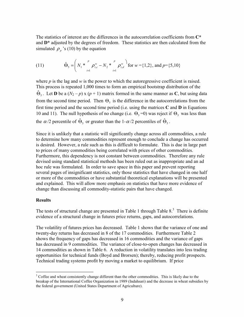
The nature of price autocorrelations has changed. Tables 7 and 8 show the fourautocorrelation measures. In 6 of the 17 commodities, at least one of the sums ofautocorrelation changed significantly. All but two of the significant changes was adecrease in autocorrelation. In addition the variance ratios in Table 3 show weakevidence of decreased autocorrelation. Under the assumption of independent andnormally distributed changes, these ratios should be near 1/p. Eight of the commoditiesshowed a significant increase in the ratios and almost all of the ratios moved closer to1/p, which indicates less autocorrelation. A majority of the technical trading systems aretrend following, and a decrease in the autocorrelation of daily returns would likelydecrease the profitability of trend following systems. While the change in price serialcorrelation is not pronounced, it is in a direction consistent with technical trading beingless profitable.

Although many market variables show evidence of change, there are still a few statisticsthat did not significantly change.4 The average size of close-to-open price changes andbreakaway gaps did not consistently change. The skewness of returns, gaps, and close-to-open changes changed in only a few commodities.

Conclusions

The returns to managed futures have decreased steadily during the past two decades;since these funds are overwhelmingly technically traded, futures prices were examinedfor evidence of a structural change that could explain the reduction in fund profitability.The results show there is evidence of a structural change in prices that may have caused areduction in the returns to managed futures funds. The two dominant changes are adecrease in price volatility and increase in large price changes occurring while marketsare closed. There was also a slight indication of reduced autocorrelation. These changesare consistent with the reduced profitability of technical trading being due to changes inthe overall economy. If prices were to again become more volatile, then presumablyreturns to technical trading would likely increase again. The reduced profitability is asignal to traders that less technical trading is now needed and presumably as technical 4 Five-minute intraday prices of six commodities were also examined, but no clear pattern of change wasfound (Kidd).

11

traders exit the market, profits will return to normal levels but not likely to the abnormallevels of the early 1980s.

References

Akgiray, V. “Conditional Heteroskedasticity in Time Series of Stock Returns: Evidenceand Forecasts.” Journal of Business, 62(1989):55-80.

Anderson, R.W. “Some Determinants of the Volatility of Futures Prices.” Journal ofFutures Markets, 5(1985):331-348.

Beja, A., and M. B. Goldman. “On The Dynamic Behavior of Prices in Disequilibrium.”Journal of Finance, 35(1980):235:248.

Billingsley, R. S., and D. M. Chance. “Benefits and Limitations of Diversificationamong Commodity Trading Advisors." Journal of Portfolio Management,23(1996):65-79.

Boyd, M. S., and B. W. Brorsen. “Sources of Futures Market Disequilibrium.” CanadianJournal of Agricultural Economics, 39(1992):769-778.

Box, G., and D. Pierce. “Distribution of Residual Autocorrelations in AutoregressiveMoving Average Time Series Models.” Journal of the American StatisticalAssociation, 65(1970):1509-1526.

Brock, W., J. Lakonishok, and B. LeBaron. “Simple Technical Trading Rules and theStochastic Properties of Stock Returns.” Journal of Finance, 47(1992):1731-1764.

Brorsen, B.W. “Futures Trading, Transaction Costs, and Stock Market Volatility.” TheJournal of Futures Markets, 2(1991):153-163.

Brorsen, B. W., and S. H. Irwin. “Futures Funds and Price Volatility.” The Review ofFutures Markets, 6(1987):118-135.

Brorsen, B.W., C.M. Oellermann, and P.L. Farris. “The Live Cattle Futures Marketand Daily Cash Price Movements.” The Journal of Futures Markets, 9(1989):273-282.

Brorsen, B. W., and J. P. Townsend. “Performance Persistence for Managed Futures.”Journal of Alternative Investments, 4(2002):57-61.

Commodity Futures Trading Commission. “Report on Cattle Futures Trading DuringMarch/April 2002.” Prepared by CFTC Market Surveillance, April 19, 2002.

12

Cornew, R.W., D.E. Town, and L.D. Crowson. “Stable Distributions, Futures Prices, andthe Measurement of Trading Performance.” Journal of Futures Markets,4(1984):531-557.

Dufour, J.M., and A. Farhat. “Exact Nonparametric Two-Sample Homogeneity Tests forPossibly Discrete Distributions.” Unpublished Working Paper CAHIER 23-2001,University of Montreal.

Edwards, F.R., and J. Liew. “Hedge Funds versus Managed Futures as Asset Classes.”Journal of Derivatives, 6(1999):45.

Efron, B. “Bootstrap Methods: Another Look at the Jacknife.” Annals of Statistics,7(1979):1-26.

Franzmann, J.R., and P.W. Sronce. “Multiple Hedging Slaughter Hogs with MovingAverages.” Oklahoma Agricultural Experiment Station Bulletin #767, 1983.

Good, P. “Resampling Methods” Class Lecture notes available athttp://ourworld.compuserve.com/homepages/quaker_phil/resamp.htm. AccessedApril 13, 2002.

Gordon, J.D. “The Distribution of Daily Changes in Commodity Futures Prices.”Technical Bulletin No. 1702, ERS, USDA (1985).

Grossman, S.J., and J.E. Stiglitz. “On the Impossibility of Informationally EfficientMarkets.” The American Economic Review, 70(1980):393-408.

Hall, J.A., B.W. Brorsen, and S.H Irwin. ”The Distribution of Futures Prices: A Test ofthe Stable Paretian and Mixture of Normals Hypotheses.” Journal of Financialand Quantitative Analysis, 24(1989):105-116.

Harri, A., and B.W. Brorsen. “The Overlapping Data Problem.” Unpublished WorkingPaper, Oklahoma State University, 2002.

Holt, B. R., and S. H. Irwin. “The Effects of Futures Trading by Large Hedge Funds andCTA’s on Market Volatility.” NCR-134 Conference on Applied Commodity PriceAnalysis, Forecasting, and Market Risk Management, Chicago, IL April 2000.

Horowitz, J.L. “The Bootstrap.” Prepared for Handbook of Econometrics, Volume 5,1999.

Houthakker, H. S. “Systematic and Random Elements in Short-Term Price Movements.”The American Economic Review, 51(1961):167-172.

13

Hudson, M. A., R. M. Leuthold, G. F. Sarassoro. ”Commodity Futures Price Changes:Recent Evidence for Wheat, Soybeans, and Live Cattle.” The Journal of FuturesMarkets, (7)1987):287-301.

Indahsari, G.K. “The Impact of International Coffee Organization on Indonesian PTPCoffee Prices.” Unpublished Masters Thesis, Oklahoma State University, 1990.

Irwin, S.H., and B.W. Brorsen. “Public Futures Funds.” Journal of Futures Markets,(5)1985:149-171.

Irwin, S. H., and B. W. Brorsen. “A Note on the Factors Affecting Technical TradingSystem Returns.” The Journal of Futures Markets, 7(1987):591-595.

Irwin, S.H., J. Martines-Filho, and D.L. Good. “The Price Performance of MarketAdvisory Services in Corn and Soybeans Over 1995-2000.” AgMAS ProjectResearch Report 2002-01, April 2002.

Irwin S. H. and J.W. Uhrig. “Do Technical Analysts Have Holes in Their Shoes?”Review of Futures Markets, 3(1984):364-277.

Kaufmann, A. “The Source of Futures Investment Returns.” Global Investor, (1993):29-33.

Kidd, W.V. “Can Structural Changes Explain the Decrease in Returns to TechnicalAnalysis.” Unpublished Masters Thesis, Oklahoma State University, 2002.

Kowalewski, M. “Bootstrap Methods.” Lecture notes for Quantitative Paleobiology.Available at http://www.cyber.vt.edu/geol5374/I12.pdf, Accessed April 30, 2002.

Ljung, G. M., and G. E. P. Box. “On a Measure of Lack of Fit in Time Series Models.”Biometrika, 65(1978):297-303.

Lo, A.W. and A.C. MacKinlay. “Stock Market Prices Do Not Follow Random Walks:Evidence from a Simple Specification Test.” Review of Financial Studies,1(1988):41-66.

Lukac, L. P., and B. W. Brorsen. “A Comprehensive Test of Futures MarketDisequilibrium.” The Financial Review, 25(1990):593-622.

Lukac, L.P., B.W. Brorsen, and S. H. Irwin. “Similarity of Computer Guided TechnicalTrading Systems.” Journal of Futures Markets, 8(1988):1-13.

Mandelbrot, B. “The Variation of Certain Speculative Prices.” Journal of Business,36(1963):394-419.

Mann, J.S., and R.G. Heifner. “The Distribution of Shortrun Commodity Price

14

Movements.” Technical Bulletin No. 1536, ERS, USDA (1976).

Maausoumi, E. “On the Relevance of First Order Asymptotic Theory to Economics.”Journal of Econometrics, 100(2001):83-86.

Osler, C.L., and P.H. Chang. “Head and Shoulders: Not Just a Flaky Pattern.”Federal Reserve Bank of New York Staff Reports, 1995.

Politis, D.N., and J.P. Romano. “The Stationary Bootstrap.” Journal of the AmericanStatistical Association, 89(1994):1303-1313.

Poterba, J.M., and L.H. Summers. “Mean Reversion in Stock Prices: Evidence andImplications.” Journal of Financial Economics, 22(1988):631-639.

Purcell, W.D. Agricultural Futures and Options: Principles and Strategies. New York,New York: Maxwell Macmillan International, 1991.

Schwager, J. D. Managed Trading Myths & Truths. New York, New York: John Wiley& Sons, 1996.

Sullivan, R., A. Timmerman, and H. White “Data-Snooping, Technical Trading RulePerformance, and the Bootstrap.” The Journal of Finance, 54(1999):1647-1691.

The Barclay Group. “Barclay CTA Index.” Available at http://www.barclaygrp.com/indices/cta/sub/cta.html. Accessed March 28, 2002.

Trevino, R.C., and T. F. Martell. “Intraday Behavior of Commodity Futures Prices.”Columbia Center for the Study of Futures Markets Working Paper No. 71. (1984).

United States Department of Agriculture. “Food and Agricultural Policy: Taking Stockfor the New Century.” Available at http://www.usda.gov/news/pubs/farmpolicy01/fpindex.htm. Accessed May 16, 2002.

White, Halbert. “A Reality Check for Data Snooping.” Econometrica, 68(2000):1097-1126.

15

-10

0

10

20

30

40

50

60

70

1980 1984 1988 1992 1996 2000

Year

Ann

ual P

erce

ntag

e R

etur

n

Figure 1. Barclay CTA index annual percentage returns by yearSource: The Barclay Group

16

Table 1. Variance of Daily and 5-Day Returns for Futures Prices.

Variance of Daily Returns Variance of 20-Day Returns

Commodity 1975a-1990 1991-2001 1975a-1990 1991-2001

Coffee 3.38 7.10++ 99.9 162.4++

Cocoa 3.57 3.16** 77.5 60.9**Corn 1.41 1.52 35.5 36.9Crude Oil 3.83 3.60 105.4 67.2Deutsche Marks 0.44 0.48 10.2 10.6Eurodollars 0.02 <0.01** 0.5 0.1**Feeder Cattle 1.14 0.53** 27.0 11.1**Gold 2.15 0.60** 45.5 12.8**Heating Oil 2.99 3.14 84.6 67.0Japanese Yen 0.43 0.58++ 11.1 12.6Live Cattle 1.33 0.60** 28.2 11.0**Pork Bellies 4.52 5.08+ 116.3 114.5Soybeans 2.25 1.48** 51.0 29.4**Standard and Poor’s 500 2.02 1.09 25.8 17.9Sugar 7.42 3.29** 160.2 66.2**Treasury Bonds 0.71 0.37** 16.9 7.3**Wheat 1.28 1.52 26.2 40.9++

a 1975 or the first date in the time series.

Notes:Hypothesis tests were performed using the two sample stationary bootstrap with 1,000 repetitions.Statistically significant increases are denoted by + at .10 level and ++ at .05 level.Statistically significant decreases are denoted by * at .10 level and ** at .05 level.

17

Table 2. Skewness and Kurtosis of Daily Returns for Futures Prices.

Skewness of Daily Returns Kurtosis of Daily Returns

Commodity 1975a-1990 1991-2001 1975a-1990 1991-2001

Coffee -0.28 0.47++ 4.05 8.08++

Cocoa 0.05 0.37++ 0.64 2.27++

Corn -0.01 -0.02 1.90 1.86Crude Oil -0.14 -2.14** 4.85 36.11++

Deutsche Marks 0.20 0.01 2.44 1.90Eurodollars 0.62 0.33 10.19 6.55Feeder Cattle -0.08 -0.07 0.46 1.04++

Gold -0.10 0.63++ 4.00 18.11++

Heating Oil -0.06 0.10 2.44 3.37Japanese Yen 0.32 0.84++ 3.13 8.62++

Live Cattle -0.10 -0.02 0.26 0.75++

Pork Bellies -0.01 0.01 -0.59 0.02++

Soybeans -0.11 -0.05 0.96 2.99++

Standard and Poor’s 500 -5.52 -0.28 158.43 5.11Sugar -0.04 -0.05 1.85 2.46Treasury Bonds 0.21 -0.36 5.80 2.06**Wheat 0.32 0.15 5.94 1.32**

a 1975 or the first date in the time series.

Notes:Hypothesis tests were performed using the two sample stationary bootstrap with 1,000 repetitions.Statistically significant increases are denoted by + at .10 level and ++ at .05 level.Statistically significant decreases are denoted by * at .10 level and ** at .05 level.

18

Table 3. Ratio of Daily Variance to 5-Day and 20-Day Variance for Futures Prices.

Ratio of Daily Variance Ratio of Daily Varianceto 5-Day Variance to 20-Day Variance

Commodity 1975a-1990 1991-2001 1975a-1990 1991-2001

Coffee 0.17 0.19+ 0.033 0.043++

Cocoa 0.18 0.21++ 0.046 0.051Corn 0.18 0.18 0.039 0.041Crude Oil 0.16 0.22++ 0.036 0.053++

Deutsche Marks 0.19 0.19 0.043 0.045Eurodollars 0.17 0.17 0.039 0.034Feeder Cattle 0.17 0.18 0.042 0.048Gold 0.19 0.20 0.047 0.046Heating Oil 0.16 0.21++ 0.035 0.046+

Japanese Yen 0.19 0.20 0.038 0.046+

Live Cattle 0.18 0.19 0.047 0.055++

Pork Bellies 0.17 0.19++ 0.038 0.044Soybeans 0.19 0.20 0.044 0.050Standard and Poor’s 500 0.25 0.22 0.078 0.061Sugar 0.20 0.20 0.046 0.049Treasury Bonds 0.18 0.20 0.042 0.051+

Wheat 0.20 0.17** 0.048 0.037**

a 1975 or the first date in the time series.

Notes:Hypothesis tests were performed using the two sample stationary bootstrap with 1,000 repetitions.Statistically significant increases are denoted by + at .10 level and ++ at .05 level.Statistically significant decreases are denoted by * at .10 level and ** at .05 level.

19

Table 4. Frequency and Mean of Breakaway Gaps in Futures Prices.

Frequency of Breakaway Gaps Variance of Breakaway Gaps

Commodity 1975a-1990 1991-2001 1975a-1990 1991-2001

Coffee 0.19 0.09** 1.73 3.12++

Cocoa 0.20 0.12** 1.14 0.41**Corn 0.16 0.10** 0.74 0.42Crude Oil 0.22 0.06** 1.65 1.43Deutsche Marks 0.26 0.15** 0.18 0.21Eurodollars 0.17 0.03** 0.01 <0.01**Feeder Cattle 0.15 0.09** 0.36 0.15**Gold 0.18 0.07** 1.05 0.19**Heating Oil 0.26 0.08** 1.49 0.81**Japanese Yen 0.39 0.09** 0.15 0.10**Live Cattle 0.13 0.06** 0.45 0.11**Pork Bellies 0.15 0.11** 2.02 2.06Soybeans 0.14 0.07** 1.02 0.84Standard and Poor’s 500 0.07 0.03** 0.28 0.34Sugar 0.19 0.09** 2.14 0.56**Treasury Bonds 0.17 0.07** 0.38 0.14**Wheat 0.16 0.15 0.28 0.40

a 1975 or the first date in the time series.

Notes:Hypothesis tests were performed using the two sample stationary bootstrap with 1,000 repetitions.Statistically significant increases are denoted by + at .10 level and ++ at .05 level.Statistically significant decreases are denoted by * at .10 level and ** at .05 level.

20

Table 5. Variance and Skewness of Breakaway Gaps in Futures Prices.

Skewness of Breakaway Gaps Kurtosis of Breakaway Gaps

Commodity 1975a-1990 1991-2001 1975a-1990 1991-2001

Coffee 0.33 3.77++ 7.34 33.27++

Cocoa 0.39 0.37 2.33 2.40Corn 0.86 1.06 11.25 8.79Crude Oil 0.15 -3.94* 25.31 42.95Deutsche Marks -0.07 -0.48 11.26 5.10Eurodollars 1.73 0.60 22.91 11.55Feeder Cattle -0.26 1.01++ 3.65 7.71++

Gold -0.09 -3.46** 9.01 30.84++

Heating Oil -0.17 4.38++ 6.85 42.02++

Japanese Yen 0.54 0.73 4.96 5.30Live Cattle -0.30 1.05++ 3.55 9.53++

Pork Bellies 0.09 -0.16 2.21 2.62Soybeans 0.15 -0.25 6.50 7.84Standard and Poor’s 500 -0.91 -1.98 6.56 13.17Sugar -0.65 1.09++ 7.23 6.44Treasury Bonds 1.41 -1.19 23.34 14.42Wheat -0.33 2.15 28.12 13.95

a 1975 or the first date in the time series.

Notes:Hypothesis tests were performed using the two sample stationary bootstrap with 1,000 repetitions.Statistically significant increases are denoted by + at .10 level and ++ at .05 level.Statistically significant decreases are denoted by * at .10 level and ** at .05 level.

21

Table 6. Mean and Variance of Close-to-Open Changes in Futures Prices.

Variance of Kurtosis ofClose-to-Open Changes Close-to-Open Changes

Commodity 1975a-1990 1991-2001 1975a-1990 1991-2001

Coffee 1.35 1.93++ 8.64 67.33++

Cocoa 1.37 0.73** 2.58 2.74Corn 0.45 0.28** 13.44 17.85Crude Oil 1.82 0.68** 11.12 25.41++

Deutsche Marks 0.23 0.14** 5.83 7.26Eurodollars <0.01 <0.01** 89.94 32.56Feeder Cattle 0.31 0.11** 7.90 12.29Gold 1.03 0.15** 9.36 86.64++

Heating Oil 1.57 0.86** 6.83 32.02++

Japanese Yen 0.26 0.09** 3.44 8.21++

Live Cattle 0.36 0.09** 4.01 7.96++

Pork Bellies 1.17 1.28 3.80 6.42++

Soybeans 0.66 0.32** 9.16 30.39++

Standard and Poor’s 500 0.66 0.11* 410.12 42.18Sugar 2.35 0.61** 6.61 7.25Treasury Bonds 0.37 0.06** 12.65 16.10Wheat 0.29 0.43+ 25.96 12.98

a 1975 or the first date in the time series.

Notes:Hypothesis tests were performed using the two sample stationary bootstrap with 1,000 repetitions.Statistically significant increases are denoted by + at .10 level and ++ at .05 level.Statistically significant decreases are denoted by * at .10 level and ** at .05 level.

22

Table 7. Sums of First 5 and First 10 Autoregressive Coefficients Times theNumber of Observations for Futures Prices.

Sum of First Five Sum of First 10Autoregressive Coefficients Autoregressive Coefficients

Commodity 1975a-1990 1991-2001 1975a-1990 1991-2001

Coffee 463.4 -61.6* 780.1 88.3*Cocoa 14.2 -57.3 53.5 -48.1Corn 76.3 20.1 395.5 257.1Crude Oil 199.7 -247.7 526.6 -291.4Deutsche Marks 54.9 25.5 286.5 47.9Eurodollars 167.2 288.2 375.2 644.5Feeder Cattle 459.2 79.4** 284.8 -188.0Gold -61.5 204.0 -38.0 111.4Heating Oil 309.1 -113.2 402.4 -91.8Japanese Yen 144.9 -61.5 503.1 53.6Live Cattle 241.0 -19.5 56.0 -375.5*Pork Bellies 349.4 -9.2** 484.5 257.4Soybeans 68.9 -256.4 183.3 -94.8Standard and Poor’s 500 -436.4 -344.8 -599.0 -438.5Sugar -6.1 76.6 102.9 -136.5Treasury Bonds 157.1 -260.2** 252.6 -229.3Wheat -187.5 174.3+ 101.2 397.0

a 1975 or the first date in the time series.

Notes:Hypothesis tests were performed using the two sample stationary bootstrap with 1,000 repetitions.Statistically significant increases are denoted by + at .10 level and ++ at .05 level.Statistically significant decreases are denoted by * at .10 level and ** at .05 level.

23

Table 8. Sums of First 5 and First 10 Squared Autoregressive Coefficients Timesthe Number of Observations for Futures Prices.

Sum of First Five Squared Sum of First 10 SquaredAutoregressive Coefficients Autoregressive Coefficients

Commodity 1975a-1990 1991-2001 1975a-1990 1991-2001

Coffee 26.0 16.4 34.8 21.6Cocoa 9.5 7.6 15.4 10.9Corn 10.9 14.3 29.1 25.0Crude Oil 53.7 36.7 72.9 40.2Deutsche Marks 4.1 4.8 9.8 13.3Eurodollars 26.9 47.6 30.6 64.5Feeder Cattle 17.2 10.2 20.6 28.7Gold 21.3 26.7 25.6 31.2Heating Oil 54.0 8.8 59.2 18.2Japanese Yen 4.3 5.5 15.8 9.6Live Cattle 7.5 7.1 21.2 22.9Pork Bellies 14.6 10.3 17.9 22.0Soybeans 2.7 13.8 8.9 20.9Standard and Poor’s 500 54.7 12.6 61.7 19.1Sugar 7.6 17.7 12.1 25.0Treasury Bonds 6.0 15.2 8.0 35.4+

Wheat 14.6 33.3 25.7 37.3

a 1975 or the first date in the time series.

Notes:Hypothesis tests were performed using the two sample stationary bootstrap with 1,000 repetitions.Statistically significant increases are denoted by + at .10 level and ++ at .05 level.Statistically significant decreases are denoted by * at .10 level and ** at .05 level.