Can Short-sellers Predict Returns?Daily Evidence

Karl B. Diether,Kuan-Hui Lee,

Ingrid M. Werner∗

This Version: August 11, 2006First Version: June 17, 2005

Comments are Welcome

Abstract

We test whether short-sellers in U.S. stocks are able to predict future returns based on new

SEC-mandated data for 2005. There is a tremendous amount of short-selling activity during

the sample: Short-sales represent 24 percent of NYSE and 32 percent of Nasdaq share vol-

ume. Our analysis shows that short-sellers primarily target short-term overreaction in stock

prices, but they are also able to detect stocks with short-term underreaction. Increasing short-

sales predict future negative abnormal returns. A trading strategy based on daily short-selling

activity generates significant positive returns.

∗All three authors are at the Fisher College of Business, The Ohio State University. We are grateful for commentsfrom Leslie Boni, Rudi Fahlenbrach, Frank Hatheway, David Musto, René Stulz, and seminar participants at the OhioState University, the NBER Market Microstructure Group, and the University of Georgia. We thank Nasdaq EconomicResearch for data. All errors are our own.

There is currently tremendous interest in short-selling not only from academics, but also from

issuers, media representatives, state and federal regulators, and from Congress and the Senate.

Academics generally share the view that short-sellers help markets correct short-term deviations

of stock prices from their fundamental value. This is consistent with examples of famous short-

sellers such as Jim Chanos of Kynikos Associates who was an early short-seller in Enron and

David Tice of the Prudent Bear Fund who was an early short-seller in Tyco International. Many

issuers do not agree. For example, Canadian drug company Biovail and Utah-based online retailer

Overstock.com accuse short-sellers of driving their stock price into the ground and have taken

their cases to court. Media representatives often characterize short-sellers as immoral, unethical

and downright un-American.1 At the federal level, new regulation governing short-sales in U.S.

markets came into effect on January 2, 2005. Feeling that the new federal regulation is inadequate,

Utah regulators recently passed a bill that clamps down on short-selling in Utah-based companies.2

Washington is also interested in short-selling, and the Congressional Committee of Financial Ser-

vices (May 22, 2003) and the Senate Judiciary Committee (June 28, 2006) have recently heard

testimonies about short-sellers and hedge funds.

In this paper, we try to shed some light on the trading strategies used by short-sellers of U.S.

stocks. We first test whether short-sellers target stocks with recent price increases (contrarian

traders) or recent price declines (momentum traders). We find that short-sellers primarily follow a

contrarian strategy. On average, they increase their short-selling activity following positive returns.

They also decrease their short-selling activity after negative returns on average. This does not

mean that all short-sellers are contrarians. We do find that a smaller group of short-sellers follow a

momentum strategy, i.e., they increase short-selling activity following negative returns. To discern

whether there is scope for short-sellers to make money on their trades, we also test whether short-

selling intensifies on days preceding negative returns. The results show that short-sellers time their

trades extremely well relative to short-term price trends, and this is true whether or not they follow

a contrarian trading strategy. Stock prices decline significantly the day following increased short-

selling activity. In fact, increased short-selling is followed by negative abnormal returns up to five

1For example, John Rothchild in the Bear Book said, “Known short sellers suffer the same reputation as the detestedbat. They are reviled as odious pests, smudges on Wall Street, pecuniary vampires.”

2In May, Utah adopted a law that fines brokers that facilitate naked short-selling. The amount can range from$10,000 a day to millions of dollars to cover all unsettled trades. The Utah law is set to take effect on October 1, 2006,but it is is currently being challenged by the Securities Industry Association (SIA).

1

days out.

How should we interpret the fact that short-sellers as a group predict short-horizon abnormal

returns? Does it mean that they have inside information about future fundamental values or are

they capable of detecting when the current price deviates from the fundamental value? The first

alternative suggests that short-sellers are either corporate insiders or are privy to advance release of

valuation-relevant information from the corporation. We find this hard to believe given how many

restrictions are levied on trading by corporate insiders. Moreover, Regulation Fair Disclosure (Reg

FD) is in effect during our sample period which should limit the ability of outsiders to get advance

access to material non-public information.

The second alternative suggests that market frictions (Miller (1977), Diamond and Verrec-

chia (1987), Harrison and Kreps (1978), and Scheinkman and Xiong (2003)) or behavioral bi-

ases (DeBondt and Thaler (1985), Daniel et al (1998), Barberis et al (1998), and Hong and Stein

(1999)) may cause price to deviate from fundamental value in the short-run, and that short-sellers

are exploiting these situations to their benefit. If short-sellers target short-term overreaction, their

strategies would appear contrarian in the data. If short-sellers target short-term underreaction, it

may either look like they follow a momentum strategy or as if their trades are unrelated to past

returns depending on how fast price is moving toward fundamental value. For this interpretation

of our evidence to work, however, short-sellers need to be more sophisticated than the average

investor. Given the cost of short-selling, short-sellers are likely to be predominantly institutional

traders. For example, Boehmer et al (2004) find that about 75 percent of all short-sales are ex-

ecuted by institutions while individuals represent less than 2 percent (the rest are specialists and

other). Since many institutions are prevented from shorting (e.g., many mutual funds), the ones

that may use short-selling as part of their strategy tend to be more sophisticated institutions. Thus,

short-sellers as a group are likely to be sophisticated traders.

We conduct a number of robustness tests to rule out alternative explanations for our findings.

We check whether short-sellers trade mechanically on well known short-term predictability in

daily returns. This type of trading would be consistent with the view that short-sellers are purely

technical traders. For example, we control for short-term return reversals (e.g., Jegadeesh (1990)

and Lehmann (1990)), for positive autocorrelation in buy order-imbalances (Chordia and Subrah-

manyam (2004)), for the volume-return relationship (e.g., Conrad et al (1994), Gervais et al (2001),

2

and Llorente et al (2002)), and for possible measurement problems using CRSP returns (Kaul and

Nimalendran (1990)). We also explore whether short-sellers are simply acting as passive liquidity

providers, so that the contrarian patterns and predictability are a direct result of short-sellers requir-

ing compensation for providing immediacy (e.g., Stoll (1978), Grossman and Miller (1988), and

Campbell et al (1993)). These alternative explanations do not eliminate the ability of short-selling

activity to predict returns.

It is worth pointing out that short-sellers are not all alike. In our stock-level aggregate data

on short-sales, we clearly have some traders that speculate on prices reverting to fundamentals.

However, we also have traders that use short-sales to hedge a long position in the same stock, to

conduct convertible arbitrage or index arbitrage, traders who seek to hedge their options positions,

etc. Many of the trading strategies involving short-sales are based on relative valuations of se-

curities (e.g., merger arbitrage) which reduces the likelihood that predictability will be found in

a regression framework. These traders may or may not be selling short because they think the

shorted stock is overvalued relative to current fundamentals. Their presence in the data will work

against us finding that stock-level aggregate short-sales predict abnormal negative returns. Yet, we

do find predictability both in the regression analysis and in the long-short portfolio analysis.

We are not the first to investigate whether short-sellers are informed traders. There is by now

a rather extensive literature studying the relationship between short-selling activity measured as a

stock variable (short-interest) and stock returns. While the earlier literature provided mixed evi-

dence, there is growing consensus that short-sellers are informed.3 For example, researchers find

that high short-interest predicts negative abnormal returns for NYSE/AMEX stocks (Asquith and

Meulbroek (1995)) and for Nasdaq stocks (Desai et al (2002)), that short-sellers target companies

that are overpriced based on fundamental ratios (Dechow et al (2001)), that short-sellers targets

firms with earnings restatements and high accruals (Efendi et al (2004), Desai et al (2005)), antic-

ipate downward analyst forecast revisions and negative earnings surprises (Francis et al (2005)),

and that short-sellers exploit both post-earnings announcement drift and the accrual anomaly (Cao

and Kolasinski (2005)).

These studies use monthly stock-specific short interest data. This data is disclosed by ex-

3For the earlier literature, see, e.g., Figlewski (1981), Brent et al (1990), Senchack and Starks (1993), and Asquithet al (2005).

3

changes around the middle of each month, and consists of the number of shares sold short (a stock

variable) at a particular point in time. There are two main problems with using monthly short inter-

est data. The first problem is that the monthly data does not permit a researcher to discern whether

or not a high level of short interest means that short-selling is more expensive, which is the pre-

requisite for the over-reaction story as proposed by Miller (1977). To remedy this short-coming

of the literature, several authors have relied on proxies for short-sale constraints or demand (Chen

et al (2002) - breadth of ownership, Diether et al (2002), Nagel (2004) - institutional ownership,

Lamont (2004) - firm’s actions to impede short-selling), and even the actual cost of borrowing

stock (D’Avolio (2002), Cohen et al (2006), Jones and Lamont (2002), Geczy et al (2002), Ofek

and Richardson (2003), Reed (2002), Ofek et al (2003), Mitchell et al (2002)) to investigate if

short-sale constraints contribute to short-term overreaction in stock prices, and if short sellers are

informed. The general conclusion reached by this literature is that short-sale costs are higher and

short-sale constraints are more binding among stocks with low market capitalization and stocks

with low institutional ownership. The literature also finds that high shorting demand predicts ab-

normally low future returns both at the weekly and monthly frequency.

The second problem is that the monthly reporting frequency does not permit researchers to

study short-term trading strategies. Recent evidence suggests that many short-sellers cover their

positions very rapidly. For example, Cohen et al (2006) find that more than half the securities

lending contracts they study are closed out in 3 weeks. Also note that if a trader sells a stock short

in the morning, he can cover the position with a purchase before the end of the day without ever

having to actually borrow the stock, suggesting that the even securities lending data truncates the

holding period of short-sellers.4 The notion that short-sellers focus on short-term trading strategies

is consistent with our finding that short-sales represent on average 24.1 percent of NYSE and 31.9

percent of Nasdaq (National Market) reported share volume. By comparison, average monthly

short interest for the same period is about 6.2 days to cover for NYSE stocks and 6.8 days to cover

for Nasdaq stocks. Hence, it is important to study short-selling activity at a higher frequency. This

is our main contribution to the literature.

Previous studies of short-selling have sought to test whether short-sellers time their trades well

relative to future returns. However, as far as we know, no one has previously examined how

4Jones (2004) finds that such “in-and-out shorting” represented about 5 percent of daily volume is the early 1930s.

4

short-sales relate to past returns. This is puzzling since the main argument for stricter short-sale

regulation is that short-sellers exacerbate downward momentum. Without evidence on how short-

sellers trade relative to past returns, it is impossible to determine whether short-sellers actually

have any impact on momentum. Our second contribution to the literature is to examine whether

short-sellers trade on short-term overreaction (contrarian traders) or on short-term underreaction

(momentum traders).

We use the regulatory tick-by-tick short-sale data for a cross-section of almost four thousand

individual stocks. While our data permits an intraday analysis of short-selling, we aggregate short-

sales for each stock to the daily level for the purpose of this study. Our paper is the first study of

daily short-selling to cover both Nasdaq and NYSE stocks. This is our third contribution to the

literature.

Our final contribution is that we rely on a very comprehensive dataset. It includes all short-

sales executed in the U.S., regardless of where the trade is printed (the AMEX, the Boston Stock

Exchange, the Chicago Stock Exchange, the NASD, Nasdaq, the National Stock Exchange, the

NYSE, or the Philadelphia Stock Exchange) for all NYSE, and Nasdaq-listed stocks. The complete

coverage is clearly important as we find that over 50 (23) percent of Nasdaq (NYSE) short-sales

are reported away from the primary listing venue during our sample period. By contrast, other

authors that study daily short-sales rely on samples that do not cover all short-sales for a particular

stock. Christophe et al (2004) focus their analysis on customer short-sales that are subject to Nas-

daq’s short-sale rules and are reported to Nasdaq’s Automated Confirmation Transaction Service

(ACT). Boehmer et al (2005) and Daske et al (2005) focus their analysis on orders entered through

NYSE’s SuperDOT system that are subject to NYSE’s Uptick Rule. According to Boehmer et al

(2005), NYSE SuperDOT captures about 70.5 percent of all NYSE reported volume. However,

they acknowledge that it is uncertain whether this trading system captures an equally large pro-

portion of short-sale volume. Moreover, as mentioned, we find that 23 percent of total short-sale

volume for NYSE-listed stocks is printed away from the NYSE, which suggests that the coverage

in these two studies may be somewhat limited.

There are a few drawbacks with our data that are worth mentioning. The main drawback

is that the sample period is short - we rely on data from January 2 - December 30, 2005 for

this study. The reason is that the regulatory data only became available starting January 2, 2005

5

(which limits us on the front end) and that we need CRSP and Compustat data for the analysis

(which limits us on the back end). However, the 2005 sample is important since we have several

reasons to believe that short-selling strategies have changed dramatically in recent years: e.g.,

increased investor pessimism following the 2000 bubble, increased use of algorithmic trading,

and a tremendous growth of the hedge-fund industry which systematically employs long-short

strategies. Nevertheless, our results should be interpreted with caution given the short sample

period.

We also do not know anything about the short-sellers in our sample other than the time, price,

and size of their trades. In an earlier draft of this paper we conducted the analysis by trade size.

However, given that institutions order-split heavily, it is doubtful whether it is possible to use

trade size to separate retail from institutional trades.5 The data also includes a flag for whether

or not a short-sale is exempt from the exchanges’ short-sale rules. This seems to be a convenient

way to separate out market maker short-sales (which are largely exempt) from customer short-

sales as done by Christophe et al (2004) and Boehmer et al (2005). However, due to a no-action

letter from the SEC, market participants have been relieved from systematically using the “short-

exempt” marking rendering the flag useless. While we have no reason to believe that market makers

are worse at detecting overreaction than other short-sellers, we are somewhat concerned that our

contrarian trading results may in large part derive from their role as market makers. Fortunately,

we are able to use the trades in one venue which does not have designated market makers (ArcaEX)

in our robustness tests. Short-sellers using ArcaEX are also contrarian and their activity predicts

future abnormal returns.

Another potential drawback with the regulatory short-sale data is that while we see each in-

dividual short-sale, the data does not flag the associated covering transactions. Hence, we cannot

determine whether short-sellers’ trades are profitable. Such data is not contained in the audit trail

from which the regulatory data is drawn and could only be obtained at the clearing level. Instead,

we have to rely on indirect measures such as whether or not it is possible to create a profitable

trading strategy based on daily short-selling activity. For this purpose, we form characteristic-

adjusted portfolios that are long stocks with low short-selling activity and short stocks with a high

activity. We find that these long-short portfolios of NYSE (Nasdaq) stocks generate significant

5For an analysis of short-sales by account type, see Boehmer et al (2005).

6

characteristic-adjusted (size–book to market) average abnormal returns of 1.06 (1.72) percent per

month when the holding period is one-day and significant average returns of 0.6 (1.24) percent

per month when the holding period is five-days. Note, however, that trading costs are likely to be

substantial because of the short holding periods.

Our results are generally consistent with the return predictability found in NYSE SuperDOT

short-sales for the 2000-2004 period by Boehmer et al (2005). They find that stocks with rela-

tively heavy shorting underperform lightly shorted stocks by a risk-adjusted average of 1.07 per-

cent in the following 20 days of trading and conclude that short-sellers as a group are extremely

well-informed. The same conclusion is drawn by Christophe et al (2004) who find that short-

selling activity in Nasdaq stocks is concentrated in periods preceding disappointing earnings an-

nouncements. Daske et al (2005) draw the opposite conclusion as they find that short-sales are not

concentrated prior to bad news disseminated by scheduled earnings announcements, unscheduled

voluntary disclosures, or substantial stock price declines for NYSE SuperDOT short-sales. These

contradictory conclusions may seem puzzling, but can possibly be reconciled by considering the

disclosure regimes in effect during the two sample periods. The Christophe et al (2004) sample

brackets the effective date of RegFD, October 23, 2000. Hence, it is quite likely that material non-

public information was communicated to select investors in advance of the earnings announcement

(e.g, in meetings between corporations, analysts, and institutional investors, at least during part of

their sample period). By contrast, the Daske et al (2005) sample is drawn from a period with much

stricter regulation on the release of material non-public information, and no predictability is found

around earnings announcements.6

Our finding are consistent with a recent paper by Avramov, Chordia, and Goyal (2005) who

study the impact of trades on daily volatility. They find that increased activity by contrarian traders

(identified as sales following price increases) is associated with lower future volatility, while in-

creased activity by herding investors (identified as buyers after price increases) is associated with

higher future volatility. Avramov et al (2005) argue that contrarian traders are rational traders

that trade to benefit from the deviation of prices from fundamentals. As these trades make prices

more informative, they tend to reduce future volatility. We provide more direct evidence of the

6An earlier draft of this paper finds that Nasdaq short-sellers are unable to predict negative earnings announcementsduring our sample period.

7

information content of contrarian short-sellers in that they predict future returns.

Our results are also reminiscent of a recent study of net individual trade imbalances on the

NYSE during the 2000-2003 period by Kaniel et al (2006). They find that individuals are con-

trarians, and that their trades predict returns up to 20 days out. However, the authors discard

the fundamental information hypothesis and instead interpret their evidence as consistent with the

liquidity provision hypothesis. The reason is largely that they find it hard to believe that individ-

ual traders are more sophisticated than institutions. As discussed above, we have good reason to

believe that short-sellers are more sophisticated than the average investor.

Our study proceeds as follows. We summarize our hypotheses in Section I, and describe

the data in Section II. We test whether short-sellers primarily trade on short-term overreaction

(contrarian) or on short-term underreaction (momentum) in Section III. We address whether

short-selling activity predicts future returns in Section IV. A number of robustness checks are

conducted in Section V. Section VI concludes.

I. Hypotheses

Our hypotheses can be summarized as follows:

u If short-sellers are contrarian traders, they trade after positive returns.

u If short-sellers are momentum traders, they trade after negative returns.

u Short-sellers are trading on short-term overreaction if they sell following positive returns and

their trades predict future negative returns.

u Short-sellers are trading on short-term underreaction if they sell following (zero or) negative

returns and their trades predict future negative abnormal returns.

u If short-sellers are well-informed, it should be possible to create a profitable long-short portfolio

based on measures of short-selling activity.

We test these hypotheses in the rest of the paper.

8

II. Characteristics of short-selling

A short-sale is generally a sale of a security by an investor that does not own the security. To

deliver the security to the buyer, the short-seller borrows the security and is charged interest for the

loan of the security (the loan fee). The rate charged can vary dramatically across stocks depending

on loan supply and demand. For example, easy to borrow stocks may have loan fees as low as

0.05 percent per annum, but some hard-to-borrow stocks have loan fees greater than 10 percent per

annum (Cohen et al (2006)). If the security price falls (rises), the short-seller will make a profit

(loss) when covering the short position by buying the security in the market.

The SEC requires an investor to follow specific rules when executing a short-sale. The rules are

aimed at reducing the chances that short-selling will put downward pressure on stock prices. Until

May 2, 2005, these rules were different for Exchange-Listed Securities (the Uptick Rule, Rule

10a-1 and 10a-2, NYSE Rule 440B) and Nasdaq National Market (NM) Securities (the best-bid

test, NASD Rule 3350). Moreover, Nasdaq NM stocks that were traded on other venues (ECNs)

had no bid-test restriction.

On June 23, 2004, the SEC adopted Regulation SHO to establish uniform locate and delivery

requirements, create uniform marking requirements for sales of all equity securities, and to estab-

lish a procedure to temporarily suspend the price-tests for a set of pilot securities during the period

May 2, 2005 to April 28, 2006 in order to examine the effectiveness and necessity of short-sale

price-tests.7 At the same time, the SEC mandated that all Self Regulatory Organizations (SROs)

make tick-data on short-sales publicly available starting January 2, 2005. The SHO-mandated data

includes the ticker, price, volume, time, listing market, and trader type (exempt or non-exempt from

short-sale rules) for all short-sales. Unfortunately, the flag indicating that a trade is “short-exempt”

has been rendered unreliable through a no-action relief letter issued by the SEC.8 The data does not

include information about subsequent covering of short-sales (i.e., purchases). In this study, we

do not examine the effects of Regulation SHO per se. However, our study is made possible by the

SEC mandated short-sale data. In related work, we study the effects of suspending the price-tests

on market quality (Diether et al (2006a)) and how the new delivery and locate requirements affect

short-sales and returns (Diether et al (2006b)).7On April 20, 2006, the SEC announced that the short-sale Pilot has been extended to August 6, 2007.8The SEC granted a no-action relief from Rule 200g of Regulation SHO (the “short-exempt” marking requirement)

for trades in Exchange Traded Funds and in pilot securities in a no-action letter dated January 3, 2005.

9

This study focuses on NYSE and Nasdaq-listed stocks. We define our universe as all NYSE

and Nasdaq National Market (NM) stocks that appear in CRSP with share code 10 or 11 (common

stock) at the end of 2004. We draw daily data on returns, prices, shares outstanding, and trading

volume for these securities for the January 2, 2005 to December 30, 2005 time period from CRSP.

We also download intraday data from all SROs that report short-sales and calculate daily short-

selling measures. Specifically, we compute the number of short sales and shares sold short. Finally,

we compute daily returns based on closing mid-quotes, daily buy order-imbalances using the Lee

and Ready (1991) algorithm, and daily time-weighted quoted spreads from TAQ.9 We merge the

daily short-sale data with return and volume data from CRSP. We then filter the sample by only

including common stocks with an end-of-year 2004 price greater than or equal to $1. We also

exclude stock-days where there is zero volume reported by CRSP.10

In addition, we obtain monthly short interest data directly from Nasdaq and the NYSE, and

data on market capitalization, book-to-market, and average daily trading volume (share turnover)

for from CRSP and COMPUSTAT. We obtain institutional ownership data as of the fourth quarter

of 2004 from Thompson Financial (13-F filings), and option trading volume data from The Options

Clearing Corporation (www.optionsclearing.com). Our final sample covers trading in 1,481 stocks

for the NYSE and 2,372 for Nasdaq. To conform with the previous literature, we perform most of

our analysis on the stocks with a lagged price of at least $5, but conduct robustness test using the

sample of low-priced stocks.

Table I illustrates the distribution of shorted shares in the top of Panel A, and the number of

short-sale trades in bottom half of Panel A by market venue: American Stock Exchange (AMEX),

Archipelago (ARCAEX), Boston Stock Exchange (BSE), Chicago Stock Exchange (CHX), Na-

tional Association of Securities Dealers (NASD),11 NASDAQ, National Stock Exchange (NSX),12

and Philadelphia Stock Exchange (PHLX). NYSE accounts for almost 77 percent of shares sold

short in NYSE-listed stocks, while NASDAQ accounts for 16 percent and ARCAEX accounts for

4 percent. NASDAQ accounts for just over half the shares sold short in Nasdaq-listed stocks, while

ARCAEX and NSX each account for roughly one-quarter. The table clearly highlights that it is im-

9Our data-set currently covers order-imbalances for February - July, 2005 (see, Diether et al (2006a)).10We also set short-sales equal to volume in the few instances where short-sales exceed reported volume. Our results

are robust to excluding these stock-days from our analysis.11NASD operates the Alternative Display Facility (ADF), where trades may be printed.12Formerly known as the Cincinnati Stock Exchange.

10

portant to consider trading outside the market of primary listing. The distribution of shorted shares

roughly mirrors the distribution of overall trading volume in NYSE and Nasdaq-listed stocks across

market venues.13 By comparing the two parts of Panel A, it can be inferred that short-sale trades

are generally larger in the market of primary listing.

Panels B and C of Table I provide descriptive statistics for our daily short-selling data. Note that

the dispersion across stock-days is significant, particularly for the Nasdaq sample. To normalize

across stocks, we define the relative amount of short-selling (relss) as the daily number of shares

sold short for a stock-day divided by the total number of shares traded in the stock during the

same day. Overall, short-selling represents 24.12 percent of share volume on the NYSE and an

astonishing 31.88 percent of Nasdaq share volume. Hence, almost one in four shares traded in

NYSE stocks and almost one in three shares traded on Nasdaq involves a short-seller. Note that

relss is much less skewed than the other measures of short-selling activity. It will be the measure

of short-selling that we use throughout this paper.

The last panel of Table I reports how average short-selling activity varies with firm charac-

teristics. The previous literature has found that short-interest tends to be higher for large-cap

stocks, for low book-to-market stocks, for stocks with high institutional ownership, and for stocks

with high turnover (D’Avolio (2002) and Jones and Lamont (2002)). We define size (ME) and

book-to-market (B/M) terciles based on NYSE breakpoints, and find that large-cap stocks and low

book-to-market stocks (growth stocks) have greater short-selling on average than small-cap stocks

and value stocks. Stocks with high institutional ownership at the end of 2004 and stocks with

high trading volume (share turnover) during 2004 (CRSP) have greater short-selling activity than

stocks with low institutional ownership and low trading volume. Our results on short-selling ac-

tivity in the cross-section are thus consistent with the previous literature. Note, however, that the

differences between the terciles are much smaller for NYSE than for Nasdaq stocks.

Since the collateral costs for low-price stocks is high (Cohen et al (2006)), we expect to see

less short-selling in these stocks. Indeed, we find that stocks with a price at or above $5 have

more short-selling than those with prices below $5. Buying put options is an alternative way to

make a negative bet on a stock, so it would seem that stocks with actively traded put options

13NYSE’s 2005 market share was 78.6 percent (www.nyse.com). In May 2005, Nasdaq traded 55.8 percent of sharevolume, Archipelago traded 18.2 percent, and NSX traded 24.8 percent (source: www.nasdaq.com).

11

should have less short-selling activity. We find the opposite - stocks with actively traded puts

(www.optionsclearing.com) have higher short-selling activity. The most likely explanation is that

stocks with actively traded puts are also likely to be larger more liquid stocks for which we know

short-selling activity is higher.

In Table II, we summarize cross-sectional information on short-sales as well as stock character-

istics. Panel A is constructed from the average daily short-sales for each stock. The cross-sectional

averages of relss are very close to the pooled cross-section time-series averages in Table I. We

have information on short interest from each market, and for comparison with relss we relate this

figure to average daily volume. Recall that 24 percent of share volume in NYSE stocks and 32

percent of daily share volume in Nasdaq stocks are short-sales. By comparison, average monthly

short-interest, defined as the stock of shorts at the middle of month t divided by average daily vol-

ume during in month t− 1, is 6.24 for the NYSE and 6.81 for Nasdaq during our sample period.

In other words, for the average stock in our sample, it would take between 6 and 7 days to cover

the entire short position if buying to cover short-sales was 100 percent of volume. While we do

not observe the covering activity, we know that it has to be of the same order of magnitude as the

short-selling.

To see why, consider the average Nasdaq stock and assume it has a (constant) average daily

volume of 100,000 shares. Further, suppose that its short interest is 4,000 shares in mid-January,

that this doubles to 8,000 shares by by mid-February, and that there were 22 trading days between

the two readings. Our numbers suggest that short-sales during the month would reach a total of

22*32,000=704,000 shares. To hit the mid-February 8,000 shares of short interest, total purchases

to cover short-sales during the month would have to be 700,000 shares, or on average 31,818 shares

per day. Note that this does not mean that virtually every short-sale on day t is covered on day t.

Denote short interest at month m by Sm, and short-sales on date t in month m by dSm, t. Further,

denote the average holding period (in days) for the current and previous month as hpm and hpm−1

respectively to get the following relationship:

Sm+1 = Sm +22

∑t=1

dSm,t −22−hpm

∑t=1

dSm,t −0

∑t=−hpm−1

dSm−1,t . (1)

The first sum is short-sales during the current month, the second sum is covering transactions of

12

short-sales during the current month that take place during the current month, and the third sum is

covering transactions in the current month of short-sales that took place in the previous month. It

follows that changes in short-interest is positively related to both to increases in holding periods

and to increases in daily short-selling activity.

Panel B of Table II reports the cross-sectional correlations between our short-sale measures

and stock-characteristics. Short-selling activity for both NYSE and Nasdaq stocks is significantly

positively correlated with institutional ownership, short interest, price, and turnover, and a dummy

for actively traded put options. In addition, short-selling activity for Nasdaq stocks is significantly

positively correlated to size. By contrast, short-selling activity is negatively correlated to B/M, and

for Nasdaq the correlation is significant. Hence, growth stocks have more short-selling activity

than value stocks.

III. How do short-sellers react to past returns?

What signals do traders use to decide when to short a stock? While providing a complete answer

to this question is beyond the scope of our paper, it is reasonable to assume that short-sellers

rely heavily on past price-patterns. The major reason for this conjecture is that virtually every

book on short-selling uses price-pattern-based technical trading rules as entry and exit signals.

Consequently, we analyze how short-sellers react to past returns. Our study focuses on short-term,

short-selling strategies. Therefore, we chose a five-day window preceding the day of the short-sale

as our period to measure returns. As described in the hypothesis section, we will first test if short-

sellers target stocks with underreaction (momentum traders) or stocks with overreaction (contrarian

traders). Recall that momentum traders are expected to increase their short-sales following negative

returns, while contrarian traders are expected to increase short-sales following positive returns.

We first compare the distribution of past returns and short-sales in Table III. The table re-

ports the mean number of stocks for short-selling (relsst) portfolios disaggregated by past returns

(r−5,−1). On date t, we compute relsst terciles for each market. On date t, we also compute return

terciles for each market. We then form portfolios from the intersection of relss terciles and past

return terciles. The numbers in the cells of Table III are the average number of stocks in each port-

folio. If all traders were contrarians (and used the weekly past returns as their trigger), we would

have the entire sample distributed along the downward-sloping diagonal of each panel. Clearly,

13

we do not. On average there are 177 NYSE (211 Nasdaq) winner stocks with high relss and 176

NYSE (209 Nasdaq) loser stocks with low relss. By comparison, there is an average of 120 NYSE

(168 Nasdaq) loser stocks with high relss and 111 NYSE (166 Nasdaq) winner stocks with low

relss. These are the cases that we associate with a momentum strategy. Thus, for both NYSE and

Nasdaq stocks, there are many more stocks where short-sellers are following a contrarian trading

pattern.

In Table IV we regress individual stock short-sales during day t (relsst) on past returns. The

panel regressions include day and stock fixed effects, and standard errors corrected for clustering

by calendar date.14 Additionally, the regressions only include stocks with lagged price greater

than or equal to $5. It is clear from the first column in Panels A (NYSE) and B (Nasdaq) that

short-selling activity increases significantly in past returns, r−5,−1. The coefficient implies that a

return over the past five days of 10 percent results in an increase in short-selling of 3.98 percent

(2.16 percent) of average daily share volume for NYSE (Nasdaq) stocks. Hence, short-sellers

are contrarian on average also in the panel regression framework. Including lagged short-sales

(relsst−1) and lagged turnover (log(tv−5,−1)) weakens the magnitude of the effect (columns three

and four), but it is still highly significant.

We explore asymmetric and possible non-linear responses to past returns in columns four and

five of Table IV. To accomplish this, we sort stocks for each market into quintiles based on their

past returns. We define a dummy that takes on a value of one for stocks in the highest (lowest)

quintile as winner (loser). Short-selling is significantly higher for past winners, and significantly

lower for past losers. Note also that the coefficients on the winner and the loser portfolios are quite

similar. In other words, short-sellers do not only short more after price increases, they also short

significantly less following negative returns. This reinforces our result that the majority of short-

sellers are contrarian, and not momentum traders. The difference between short-selling of past

winners and past losers is 5.1 percent (3.9 percent) of average daily volume for NYSE (Nasdaq)

stocks. These differences are highly significant based on an F-test (not reported). Controlling

for past short-selling activity and turnover reduces the magnitude of the coefficients, but does not

change our conclusion that the majority of short-sellers in both markets are contrarian.

14The results are very similar if we use firm characteristics instead of stock fixed effects.

14

IV. Can short-sellers predict future returns?

For the shorting strategy to be successful, the stock price has to decline in the future so that the

short-seller can cover her position and still make profits large enough to cover trading costs and

costs related to short-selling. In other words, increased short-selling activity should predict future

abnormal negative returns.

The problem is that we cannot observe the actual covering transactions. We do not know

whether short-sellers keep their positions open for one day, a week, a month, or even several

months. We are also restricted in that our sample period is short, only one year. To be very

conservative, we start by examining if a significant increase in today’s short-selling activity is

associated with a significant negative abnormal return tomorrow. The short window for measuring

short-selling activity (one day) and the short horizon (one day) will make it very difficult to find

predictive power.

Tables V.A and V.B report the results of panel regressions with day fixed effects and standard

errors corrected for clustering by calendar date for NYSE and Nasdaq stocks respectively. We

regress returns on day t + 1 on relss for day t.15 The regressions only include stocks with lagged

price greater than or equal to $5. Since previous research (Fama and French (1992)) has pointed

out that size and book-to-market help explain the cross-section of average returns (and may proxy

for risk factors) we control for size (log(ME)) and book-to-market, (log(B/M)) on the right hand

side. We also know that momentum helps explain the cross-section of average returns (Carhart

(1997)), so we control for the past year’s momentum defined as r−250,−6. Note that in our short

sample, only momentum is significantly related to future returns.

In the first column of Tables V.A and V.B, we report the results of regressing future returns on

short-sales as a fraction of average daily volume, relss. Clearly, higher short-selling today predicts

a future decline in abnormal returns. The economic magnitude of the effect is also significant.

From Table I we know that the standard deviation of relss is 12.49 percent for NYSE and 18.35

percent for Nasdaq stocks. Hence, a one standard deviation increase in relss predicts a 0.0236

(0.0380) percent decline in next day characteristic-adjusted returns for NYSE (Nasdaq) stocks.

This corresponds to a monthly abnormal return of -0.52 percent for NYSE stocks and -0.84 percent

15We have also run these regressions using the Fama-MacBeth (1973) methodology with Newey-West (1987) correctstandard errors, and the results are very similar.

15

for Nasdaq stocks.

One concern may be that there is significant positive autocorrelation in short-sale activity,

which may itself cause prices to decline on day t + 1. It turns out that while short-sales are posi-

tively correlated in our sample, the effect does not eliminate the predictive ability of today’s short-

sales. Acknowledging that column two is not a predictive regression, we experiment by including

the next day’s short-sales on the right hand side. The results show that if short-sales are high tomor-

row, returns are actually significantly higher. Once we control for this pattern, higher short-sales

today are associated with a larger and much more significant negative return. The reason for these

results is that short-sellers are contrarian on average. Hence, they sell following positive abnormal

returns. Putting future short-sales in the regression helps separate days when short-sellers are still

building a position (positive future returns) from the days when short-sellers reduce their activity

(negative future returns).

We control for five-day past returns in column three. High past returns do predict negative

future characteristic-adjusted returns for Nasdaq stocks, but this effect does not eliminate the sig-

nificance of short-selling activity as a predictor of future returns. We refine the tests in columns

four to eight in Tables V.A and V.B by allowing for non-linear effects. Stocks are first sorted into

quintiles based on five-day past returns. We define a dummy variable winner (loser) to be one for

all stocks in the highest (lowest) quintile of past returns. Past returns do not predict future returns

for NYSE stocks in Table IV.A, but they are important for Nasdaq stocks in Table IV.B. Specifi-

cally, losers outperform winners, and the magnitude is 0.105 percent per day, or 2.34 percent per

month. Yet, high short-selling activity remains a significant predictor of negative future returns.

We also sort stocks into quintiles based on short-selling activity on date t and define a dummy

variable high (low) that takes a value of one for stocks in the highest (lowest) quintile of relsst .

The regressions in columns five through eight introduce these dummies in lieu of the continuous

relss variable. For both NYSE and Nasdaq, stocks in the highest quintile of short-selling activity

experience significant negative future returns by about 0.04 percent per day. By contrast, the lowest

quintile of short-selling activity predicts positive future returns for both NYSE and Nasdaq stocks.

The difference in predicted future returns for the high minus the low quintiles is significant, and

is 0.069 percent per day (1.53 percent per month) for NYSE and 0.108 percent per day (2.40

percent per month) for Nasdaq stocks. Column six controls for both non-linearities using both past

16

short-selling activity and past return quintiles. The conclusions do not change.

Columns seven and eight of Tables V.A and V.B go one step further. They compare the returns

to a contrarian and a momentum strategy. Recall that contrarian traders should increase short-

selling activity when abnormal returns are high, and decrease short-selling activity when abnormal

returns are low. Hence, the return to a contrarian strategy can be captured by the difference between

the high ∗winner and the low ∗ loser portfolios. Similarly, the return to a contrarian strategy is

captured by the difference between the high ∗winner and the low ∗ loser portfolios. For both

markets, the interaction term high ∗winner is significant and negative and the interaction term

low∗ loser is positive and significant. The spread between the portfolios in the contrarian strategy

is 0.131 percent per day (2.86 percent per month) for NYSE stocks and 0.228 percent per day

(5.02 percent per month) for Nasdaq stocks. By comparison, the spread between the portfolios

in the momentum strategy is 0.046 percent per day (1.012 percent per month) for NYSE stocks

and 0.013 percent per day (0.286 percent per month) for Nasdaq stocks. It also follows from

the results in specification seven that it is much more important to pick the right losers than to

pick the right winners. The spread between the low ∗ loser and high ∗ loser (low ∗winner and

high ∗winner) portfolios is 0.121 (0.066) percent per day for NYSE stocks. This pattern is even

stronger for Nasdaq stocks, with a spread between the the low∗ loser and high∗ loser (low∗winner

and high∗winner) portfolios portfolios of 0.181 (0.034) percent per day.

We control for both direct effects and interaction terms in specification eight. Note that it is

necessary to add up the coefficients to make sense of the results. For, both NYSE and Nasdaq

stocks the direct effect (low-high) is statistically significant (F-test not reported in table). Also, the

direct effect soaks up all the explanatory power for Nasdaq stocks, but for NYSE stocks the high∗

winner interaction term remains significant and negative. Taken together, the evidence suggests

that a contrarian short-sale strategy generates larger negative abnormal returns. However, short-

sellers relying on a momentum strategy are also able to generate significant negative abnormal

returns, and this is particularly the case for NYSE stocks. For example, the total effect for a high–

loser (high short-selling activity and low past returns) is

high+ loser +high∗ loser =−0.02%+0.016%+−0.034% =−0.038%

17

per day and the effect is significant (F-test not reported in the table). Taken together, these re-

sults suggest that short-sellers time the market well regardless of whether they are contrarian or

momentum traders.

Previous research has found that there is strong evidence of daily and weekly return reversals

in U.S. data (e.g., Jegadesh (1990) and Lehmann (1990)) and that shocks to trading volume is

related to positive future returns (e.g., Conrad et al (1994), Gervais et al (2001), and Llorente et al

(2002)). If short-sellers are technical traders, they may simply trade on either of these well-known

patterns in the data. We are interested in finding out whether short-sellers trade on short-term

deviations of price from fundamentals, which suggests that they based their trades not only on

past returns and/or volume. Therefore, we add day t returns (rt) and turnover (log(tv−5,−1) as

additional control variables. In addition, we add a measure of a shock to turnover, ∆tv, which is

defined as turnover on date t divided by the average turnover for the past month. The coefficient

on rt is consistently negative and highly significant. The daily return reversals are twice as high

and about four times as significant for Nasdaq compared to NYSE stocks, suggesting that short-

term reversals are particularly strong on Nasdaq. High turnover in the previous week does indeed

predict high characteristic-adjusted returns for both markets. More importantly, a positive shock

to turnover today is associated with positive abnormal returns tomorrow. Our conclusions that

high short-sales predict negative characteristic-adjusted returns do not change by including these

additional control variables.

If returns are predictable, it is at least potentially possible to develop a profitable trading strat-

egy based on the information in the Regulation SHO short-sale data. To investigate this, we move

to a portfolio approach. This analysis has the added benefit that it does not restrict the relationship

between short-selling activity and future returns to be linear. We first compute relss quintiles for

each market on date t and form portfolios on day t using stocks with a closing price on day t− 1

greater than or equal to $5. We then compute size and book-to-market adjusted returns based on the

standard 25 Value-weighted portfolios (Fama and French (1993)) on day t + 1 for each portfolio.

The relss portfolios are value-weighted and rebalanced daily.

Table VI summarizes the results. First note that abnormal returns tend to decline in short-

selling as a fraction of trading volume for each market (Panel A). The last column provides the

18

difference in returns between the Low and High relss portfolios in percent per day.16 A strategy

of going long the Low relss portfolio and short the High relss portfolio (Low-High) generates a

statistically significant daily average return of 0.053 percent per day (1.17 percent per month) for

NYSE stocks and 0.086 percent per day (1.91 percent per month) for Nasdaq stocks. If we extend

the holding period to five days using the overlapping holding period methodology of Jegadeesh

and Titman (1993), the portfolios generate an average daily return of 0.029 percent per day (0.64

percent per month) for NYSE and 0.062 percent per day for Nasdaq (1.37 percent per month).

The five-day returns are significant for Nasdaq stocks, but only marginally significant for NYSE.

Figure 1 illustrates the daily holding-period returns for Low-High relss portfolio based on NYSE

stocks in the top panel and Nasdaq stocks in the bottom panel. While the holding period returns

decline over time, they are positive throughout and we only lose significance for the NYSE on day

t +5.

Recall that we found evidence of strong short-term return reversals particularly on Nasdaq in

Table V. In part, this can be a result of bid-ask bounce in CRSP closing price data (Kaul and

Nimalendran (1990)). While our conclusions did not change once we corrected for short-term

return reversals in Table V, we would like to verify that our portfolio results are not driven by bid-

ask bounce. Therefore, we rerun the analysis based on closing mid-quote returns in Panel B. The

magnitudes of our Low-High relss portfolio returns decline somewhat, but the significance does

not go away. In other words, our conclusions of return predictability are robust to errors introduced

by bid-ask bounce.

The average return on Low-High strategy may seem “too large,” but execution costs and com-

missions are likely to be significant because of daily rebalancing. Moreover, we need to take the

cost of shorting into account. With effective spreads of around 30-60 basis points, execution costs

for the Low-High portfolio with the five-day holding period would be roughly 2.7-5.4 percent per

month (not including commissions).17 By comparison, explicit costs of shorting are relatively

small. Cohen et al (2006), estimate these costs to be 3.98 percent per year (0.326 percent per

month) for stocks with market capitalization below the NYSE median.18 Thus, unless a trader

16Two-thirds to three-quarters of the stocks in the Low relss portfolio have zero short-sales for the day of portfolioformation.

17Assuming that the twenty percent of the Low and 20 percent of the High portfolio turns over each day and thatthere are 22 trading days in a month, the turnover rate during the month is roughly 9 (0.20*2*22=8.8).

18This estimate is almost certainly too high for our sample since it is for stocks below the NYSE median. Our

19

managed her costs very effectively (maybe through the use of limit orders), she could easily wipe

out the positive return from a Low-High portfolio strategy.

V. Robustness tests

In this section, we conduct a number of robustness checks that explore the determinants of short-

selling activity, whether short-sellers are technical traders, whether our results derive from a subset

of stocks, whether our results are driven by market making, and whether our results are different

for the pre compared to the post Regulation SHO period.

A. The determinants of short-selling activity

We have established that short-sellers are contrarian when past returns are measured at the weekly

frequency. However, it is not clear that this is the “right” horizon.19 To better understand the joint

dynamics of past returns and relss, we include each lagged return separately in Table VII. For

completeness, we also include the contemporaneous return, rt . The regressions control for stock

and day fixed effects, and standard errors allow for clustering by date. These regressions cover a

slightly smaller sample for a six month period, February - July, 2005.20

The first column in each panel of Table VII shows that the coefficient on each individual daily

return is positive. Since we find a strong contemporaneous relationship between returns and short-

selling, we also control for daily past relss in the second column of each panel. The coefficients

on past relss on date t are all significant and positive. Moreover, once we control for past relss,

only three lags of returns are significant for NYSE stocks and four lags for Nasdaq stocks. We

interpret this as indirect evidence that deviations from fundamentals last slightly longer for the

average stock on Nasdaq compared to the average stock on the NYSE. Based on this evidence, a

weekly past return measure seems reasonable.

Chordia and Subrahmanyam (2004) find that buy order-imbalances are positively autocorre-

lated, and that high buy order-imbalances on day t− 1 predict positive abnormal returns on day t

portfolios include the cross-section of all NYSE and Nasdaq National Market stocks and our portfolios are value-weighted.

19We thank an anonymous referee for pointing this out.20We are currently computing buy-order imbalance data for the entire sample. This sample is drawn from Diether,

Lee, and Werner (2006a).

20

for NYSE firms. They argue that the predictability can be explained by order-splitting. Could our

results be driven by short-sellers trading on the positive autocorrelation in order flow? To trade

on this pattern, short-sellers should sell when observing negative contemporaneous (and past) buy

order-imbalances. The third column in each panel of Table VII shows that contemporaneous and

past (buy) order-imbalances are positively related to relss. This is the opposite of what we would

expect based on the autocorrelation in order flow in our sample (which is positive), and Chordia

and Subrahmanyam’s (2004) evidence on order flow and future returns.21

In the last column of each panel in Table VII, we control for the joint dynamics of returns, short-

selling activity, and order flow. There is virtually no effect on the coefficients on returns and past

relss of including order flow. In other words, the short-sellers are not just trading on patterns in past

order flow. Once we control for past returns and short-selling activity, only the contemporaneous

buy order-imbalance is positively related to relss. The effect of contemporaneous order flow on

relss is much stronger on NYSE than on Nasdaq which is to be expected since the Uptick Rule

forces short-sellers in NYSE stocks to act as liquidity providers.

Are short-sellers liquidity providers?

The evidence presented so far is consistent with short-sellers trading on short-term deviation of

price from fundamentals. The majority of our short-sellers sell short after observing a period of

abnormal positive returns. In other words, they seem to be trading on short-term overreaction.

This same pattern could in principle result from short-sellers acting as voluntary passive liquidity

providers (e.g., Stoll (1978), Grossman and Miller (1988), and Campbell et al (1993)).22 If it is

temporary buying pressure that causes prices to increase, we expect higher buy order-imbalances

and wider spreads to be associated with high levels of short-selling. This story suggests that we

should include not only order flow, but also spreads in our panel regressions. We test for this in

Table VIII. To economize on space, we start with the base-case in Table IV. In other words, we do

not include each lag individually. However, we do include contemporaneous explanatory variables

this time.21We verify that buy order-imbalances are positively autocorrelated during our sample period. We also replicate

Chordia and Subrahmanyam (2004) for our sample. Regardless of whether or not we include the contemporaneousbuy order-imbalance, returns are negatively correlated to past buy order-imbalances at all lags during our sample.

22We thank an anonymous referee for pointing this out.

21

The first column in each panel includes the base case, which is essentially the specification in

Table VII with the addition of time-weighted quoted spreads, spreadt , contemporaneous returns,

rt , and the contemporaneous buy order-imbalances, oimbt . We allow the explanatory variables

to shift between the pre and the post Regulation SHO periods using a dummy variable post that

takes on a value of one for the period after May 3, 2005 and a dummy variable pilot that takes

on a value of one for stocks which are now traded without price-tests. The reason is that Diether

et al (2006a) show that significant changes in market quality were associated with the change in

regime, particularly for NYSE pilot stocks. First, note that including these additional controls does

not change our conclusion that short-sellers are contrarian on average. The estimated coefficient

on r−5,−1 is positive and highly significant in all specifications. Short-sales are more responsive

to past returns for pilot NYSE stocks after price-tests are lifted, suggesting that it is now easier

to execute short-sales. We also know from the previous table that relss is higher on days with

high positive returns, and this effect is even larger for NYSE pilot stocks after price-tests are

lifted. Again evidence that lifting the Uptick Rule makes it easier for short-sellers to execute their

strategies. Finally, five-day turnover is negatively related to relss, and again the effect is magnified

for NYSE pilot stocks after May 3, 2005.

Short-selling activity is significantly lower on days with wide spreads for NYSE stocks, but

significantly higher on days with wide spreads for Nasdaq stocks. However, the coefficient on the

interaction term post ∗ pilot ∗ spread is large and positive for both markets and large enough for

NYSE stocks to counteract the coefficient on spread. This suggests that the negative relationship

between spreads and relss for NYSE stocks is directly related to the Uptick Rule. The reason

is that short-sellers on the NYSE are restricted by the Uptick Rule to passive trading strategies.

To sell a large number of shares short, they would have to compete aggressively with the other

liquidity-providers on the ask-side of the market. This tends to narrow the spread. The bid-test in

effect on Nasdaq is much less restrictive (Diether et al (2006a)), and short-sellers are able to use

more aggressive trading strategies. As a result, it is natural that a large amount of short-selling is

associated with wider spreads.

We have already seen that contemporaneous order-imbalances and relss are positively corre-

lated, but the results in Table VIII show that the effect is much smaller for pilot stocks after the

price-tests were lifted. The effect is particularly large for NYSE stocks. This pattern can also be

22

attributed to the Uptick Rule as high short-selling activity is mechanically associated with high buy

order-imbalances during the pre Regulation SHO period (Diether et al (2006a)).

In the second and third columns of each panel in Table VIII, we test whether our contrarian

story is really a liquidity-provision story in disguise. If the voluntary liquidity provision is what

drives our results, we would expect that the effect of r−5,−1 on relss should be concentrated on

days with high spreads or high oimb. In other words, if we introduce an interaction term between

r−5,−1 and spreads and oimb respectively, these terms should reduce both the coefficient and the

significance of the direct effect of r−5,−1 on relss. The results in columns two and three do not

support this conclusion. While the interaction term in column to is significant for NYSE stocks, and

the interaction term in column three is significant for Nasdaq stocks, introducing these interaction

terms does not change the magnitude of the direct effect significantly.

According to the liquidity-provision story, spreads should widen for short-sellers to be induced

to trade as voluntary liquidity providers. We have shown that absent price-tests, wide spreads

are indeed associated with higher short-selling activity. However, these results do not discern if

the spreads are wider because of buying-pressure or because short-sellers are aggressively hitting

the bid-side of the market. If spreads are wide because of buying-pressure, we should find that the

interaction term spreads∗oimb is significant and positive. By contrast, if spreads are wide because

of aggressive trading by short-sellers, the interaction term spread ∗ oimb should be negative. We

test this in the last column of each panel is Table VIII. The results are mixed. We find a significant

effect for Nasdaq stocks, but an insignificant effect for NYSE.

B. Are short-sellers technical traders?

Technical traders develop trading strategies based on regular patterns in past prices and volume.

Could it be that short-sellers are simply technical traders. Do short-sellers form their trading strate-

gies based on patterns of short-term return predictability that has been found in the literature? For

example, Jegadeesh (1990) and Lehmann (1990) find short-horizon return reversals, Conrad et al

(1994), Gervais et al (2001) and Llorente et al (2002) find that high trading volume is system-

atically related to future positive returns, and Chordia and Subrahmanyam (2004) find that high

buy order-imbalances predict future positive returns. To some degree, our panel regressions in

Tables V.A and V.B control for turnover and past returns. However, one drawback is that the panel

23

regressions assume a linear relationship between predictive variables and returns. We therefore

move to a portfolio setting to analyze this question further.

In a portfolio setting, we cannot rely on stock fixed effects to take out stock specific averages

of variables such as turnover and spreads. Unadjusted, these variables will act as cross-sectional

liquidity measures and we will just be able to pick up differences in returns for stocks of different

liquidity within our sample period. To remedy this, we compute ∆turnover (∆spread) as the ratio

between the turnover (spread) for a particular stock on date t and the average turnover (spread) for

the same stock during the previous month. The new variables are simple measures of unexpected

shocks to turnover and spreads respectively.

To test whether technical trading based on these well-known patterns are what generates pre-

dictability in our sample, we examine returns on portfolios constructed from independent sorts into

terciles of short-selling activity, and terciles of momentum, returns, shocks to turnover, shocks to

spreads, and buy order-imbalances respectively. We then form value-weighted double-sort portfo-

lios based on the intersection of these measures on day t and compute the return for the portfolios

on day t + 1. We rebalance the double-sort portfolios daily. Furthermore, we form a long-short

portfolio by buying stocks with low short-sale activity, and shorting stocks with high short-sale

activity. If short-sellers are mechanically trading on one of these patterns, there should be no

evidence of predictability from relss once we control for the pattern in question.

The results are reported in Table IX, and the table is condensed to report on the difference

in the Low-High relss portfolios for each tercile of the individual control variables. Abnormal

returns are computed by characteristically adjusting returns using 25 value-weight size-BE/ME

portfolios. The results that control for five-day momentum are in Panel A. The Low-High relss

portfolio generates significant positive returns for the Loser portfolios in both markets, and also

for the middle tercile portfolio for Nasdaq stocks. This is consistent with our previous evidence

(Table V) that it is relatively more important for short-sellers to target the right losers.

In Panel B, we control for the previous day’s return (short-term reversals). The Low-High

relss portfolio generates positive abnormal returns for the Loser tercile for Nasdaq stocks but the

results are weaker for NYSE stocks. Instead, the Low-High relss portfolio generates positive and

significant returns for NYSE stocks in the Winner tercile. Thus, on the NYSE, it seems to be more

important for short-sellers to know which stocks with positive previous day’s returns to target.

24

Panels C and D of Table IX show that the Low-High relss portfolios generate significant pos-

itive returns for the middle and High terciles of shocks to turnover and shocks to spreads in both

markets. The turnover result makes sense since deviations from fundamentals are likely to be as-

sociated with high levels of trading activity. The spread result are also reasonable since spreads are

likely to widen when there is more uncertainty about the future value of the stock. These are also

likely to be periods when we may observe price-deviations from fundamentals.

Finally, Panel E shows that Low-High relss portfolios generate significant positive returns for

the Low (Low and Middle) tercile of buy order-imbalances for NYSE (Nasdaq) stocks. Thus, the

evidence suggests that short-sellers are particularly successful at picking which stocks to sell short

among stocks with strong selling pressure. Note that this pattern is inconsistent with a liquidity-

provision story.

In sum, the results in Table IX show that short-sellers are not simply technical traders that

benefit from trading on short-term predictability of stock returns. Instead, the results are consistent

with the view that short-sellers are well-informed. Short-sellers seem to be able to detect, and act

on, deviations of price from fundamental value.

C. Cross-sectional differences in short-selling

It is quite likely that the relationship between short-selling and past returns, as well as the ability

of short-sellers to time their trades before negative returns, varies significantly in the cross-section.

For example, since we know from the previous literature that it is easier to sell short in larger firms,

in more liquid firms, and in firms with higher institutional ownership, it is likely that short-selling

is more sensitive to past returns for these stocks.

To economize on space, we combine Nasdaq and NYSE stocks together. We then sort the

stocks into terciles based on lagged market capitalization (previous month end). The breakpoints

are determined by NYSE stocks. We contrast the effect of past returns on short-selling for small-

cap and large-cap stocks in Panel A of Table X. The overall contrarian pattern of short-sales is

present and significant both for small-cap and large-cap stocks. As expected, the magnitude of the

coefficient on relss is more than twice as large for large-cap stocks compared to small-cap stocks.

Clearly, it is easier (and almost certainly cheaper) for short-sellers to establish a short position in

large-cap stocks all else equal.

25

The previous literature has tested and confirmed the Miller (1977) hypothesis that short-selling

demand seems higher for growth stocks than it is for value stocks (Jones and Lamont (2002)). We

divide our sample into growth stocks (lowest B/M tercile) and value stocks (highest B/M tercile)

based on NYSE breakpoints. Table X Panel B reports the results. There is a strong contrarian

pattern both in growth and value stocks, and as expected the magnitude and significance of the

coefficient on relss is higher for growth than for value stocks.

The previous literature has shown that stocks with high institutional ownership are less costly

to short, all else equal (D’Avolio (2002)). The suggested reason for this in the literature is that

institutions are more likely to be willing to lend stock. Hence, we divide the sample based on insti-

tutional ownership to examine if our results are driven by stocks with high institutional ownership.

The results are in Panel C of Table X. We find that short-sellers are contrarian both in stocks with

high and low institutional ownership, but as expected, the magnitude of the effect of past abnor-

mal returns on future short-sales is more than two times as high for stocks with high institutional

ownership.

Several authors (Brent, Morse, and Stice (1990), Danielsen and Sorescu (2001), Chen and

Singal (2003), and Senchak and Starks (1993)) have explored the interaction between the options

market and the stock market to investigate the extent to which short-sale constraints are binding. A

trader that wants to express a negative view about a security can either sell the security if he happens

to own it, sell the security short, or buy at the money put options. So, for stocks with actively

traded put options, there are more alternatives to bet on a decline in stock prices.23 Therefore,

we conjecture that short-selling should be less sensitive to past returns for stocks with actively

traded put options. To test this hypothesis, we download daily put option trading volume from the

Options Clearing Corporation (www.optionsclearing.com), and divide the sample into stocks with

and without traded put options.24 Panel D of Table X reports the results. Whether or not a stock

has put options, traders are strongly contrarian on average.

To complete the picture, we also consider whether our return predictability is concentrated

in firms with certain characteristics by conducting double-sorts on relss and market capitalization,

book-to-market, institutional ownership, and options trading respectively. We form value-weighted

23In addition, they could use single stock futures. However, these are relatively illiquid.24Note that there could be significant OTC trading in put options for securities where there is no activity on the

options exchanges, which will reduce our chances of finding a significant result.

26

double-sort portfolios based on the intersection of these measures on day t and compute the return

for the portfolios on day t +1. We rebalance the double-sort portfolios daily. Furthermore, we form

a long-short portfolio by buying stocks with low short-sale activity, and shorting stocks with high

short-sale activity. If there is information in the amount of short-selling, these portfolios should

generate positive and significant abnormal returns.

The results are in Table XI. As before, we pool Nasdaq and NYSE stocks for this analysis.

Abnormal returns are computed by characteristically adjusting returns using 25 value-weight size-

BE/ME portfolios. The evidence shows that significant abnormal returns are generated by long-

short relss portfolios for all sub-samples except for large caps. The magnitude of the abnormal

returns that can be generated by forming portfolios on past relss are higher for small cap stocks,

stocks with high book-to-market, stocks with low institutional ownership, and stocks with no ex-

change traded put options. By and large, these are the stocks where it is more likely that we will

observe short-term overreaction. Hence, these results provide further corroborating evidence that

short-sellers primarily target firms with short-term overreaction.

D. Short-selling on Archipelago’s Trading System

In principle, we do not take a stance on whether our contrarian-cum-predictability results are gen-

erated by market makers or by other traders. We find the results equally interesting either way.

However, a skeptic may attribute our findings to trading by market makers, as market makers have

a tendency to trade in a contrarian way due to their role as intermediaries. Unfortunately, as men-

tioned in Section I, we cannot reliably separate out market maker trades based on the regulatory

data.25

However, we can try to test whether it is market makers that create these patterns by studying

short-selling in a venue that does not have designated market makers, and where market makers are

unlikely to execute their proprietary trading - Archipelago’s ArcaEX. During our sample period,

ArcaEX executed almost 23 percent of short-sale volume in Nasdaq stocks (Table I). The ArcaEX

25The marking rules of Regulation SHO (Rule 200) orders market centers to mark short-sales as “short” or “short-exempt.” Short-exempt trades include short-sales by Nasdaq market makers and options market makers when hedgingtheir positions). However, the SEC has granted no-action relief to allow broker-dealers to mark “short,” rather than“short-exempt” for short sale order in Pilot securities and in ETFs. See, Diether, Lee, and Werner (2006a) for a moredetailed discussion.

27

sample is interesting for another reason. ArcaEX did not enforce Nasdaq’s bid-test during our

sample period so there were no constraints that pushed short-sellers to be passive in this venue.

We repeat our basic analysis for the sub-sample of short-sales in Nasdaq stocks that were

executed on ArcaEX in Table XII. The results in Panel A show that short-sellers on ArcaEx are

strongly contrarian. Panel B shows that short-sellers on ArcaEX are able to predict returns. Finally,

Panel C of Table XII shows that a portfolio that is long stocks with low levels of short-selling on

ArcaEX and short stocks with high levels of short-selling on ArcaEX generates positive abnormal

returns of 0.078 percent per day (1.73 percent per month). Hence, it appears that our patterns of

contrarian trading and predictability do not solely derive from market making activities.

E. Pre and Post Regulation SHO

Finally, we re-run the analysis for the period January 3 - April 29 and May 2 - December 30

separately. There are three reasons for this. First, given the recent changes in short-sale rules

(Regulation SHO), we are somewhat concerned that the relationships between short-sales and past

and future returns are time-varying during our sample period. Second, we want to examine whether

the fact that the price-tests for short-sales were eliminated for a subset of the stocks (pilot stocks)

significantly affects the short-sale patterns we observe for the overall sample. Third, four major

market participants were recently fined for violating Regulation SHO, and most of those violations

occurred in the first part of 2005.26

The results are in Table XIII. The results in Panel A show that short-sellers in both Nasdaq and

NYSE stocks are contrarian in both sub-periods. Note also that short-sales on the NYSE is much

more sensitive to past returns for NYSE pilot stocks after the Uptick Rule was eliminated for these

same securities. This suggests that the Uptick Rule does make it more difficult for short-sellers to

trade on short-term overreaction. No such effect is detected for Nasdaq pilot stocks, which should

come as no surprise as Diether, Lee, and Werner (2006a) conclude that Nasdaq’s bid-test is not

very restrictive.

Panel B shows that predictability is only marginally significant for the post Regulation SHO

period for NYSE stocks and the coefficients on relss decline. However, this change does not

26Daiwa Securities Inc., Goldman Sachs Execution & Clearing, Citigroup Gobal Markets Inc. and Credit SuisseSecurities were fined a total of $1.25 million by the SEC on July 24, 2006.

28

seem to have anything to do with the fact that the Uptick Rule was eliminated for Pilot stocks.

By contrast, relss remains a strong predictor of future returns for Nasdaq stocks throughout both

periods. Also in this case, both the magnitude and the significance of the coefficients on relss is

smaller in the second sub-period. No significant difference is detected for those stocks that are

no longer subject to Nasdaq’s bid-test. There is no way from our sample to figure out whether

the somewhat weaker results on predictability in the second half of 2005 (particularly for NYSE

stocks) is due to seasonal variation in predictability or a secular decline in predictability. Only time

will tell.

VI. Conclusions

We investigate how short-sellers respond to past returns, and if their trades predict future negative

abnormal returns. We find strong evidence that short-sellers in both NYSE and Nasdaq stocks are

primarily contrarian traders. They increase their short-selling activities after positive returns, and

reduce their short-selling following negative returns. This trading pattern is consistent with short-

sellers that target stocks with short-term overreaction (e.g., Miller (1977) and Hong and Stein

(1999)). However, there are also occasions when short-sellers increase their short-selling after

negative abnormal returns and decrease their short-selling after positive abnormal returns. This

trading pattern is consistent with short-selling that targets stocks with short-term underreaction

(e.g., Daniel et al (1998)). We find that increased short-selling activity predicts negative abnormal

future returns, as much as five days out. Both contrarian and momentum strategies seem to deliver

predictability, although the results are stronger for contrarian strategies.

While short-sale data is not available at a high enough frequency to actually trade on the data

we analyze, we find that a hypothetical trading strategy that goes long in stocks with low short-

selling activity and sells short stocks with high short-selling activity would generate significant

positive abnormal returns. However, given the high turnover that such a trading strategy would

entail, these positive returns could easily be wiped out by trading costs and the cost of shorting.

Nevertheless, this is strong evidence that short-sellers are able to detect, and act on, short-term

deviations of price from fundamental value.

Taken together, our results show that short-sellers are not the villains they are made out to

be by media and issuers. Instead, traders do seem to target stocks where prices are out of line

29

with fundamental value. Hence, the evidence is consistent with short-sellers helping correct short-

term overreactions and underreaction of stock prices to information. The fact that short-sellers are

relatively more successful at predicting returns for stocks that are more likely to have pricing errors

(small-cap stocks, less liquid stocks, stocks with low institutional ownership, and stocks without

put options) is further suggestive evidence that short-sellers may actually help make prices more

efficient.

30

References

Asquith, P., and L. Meulbroek, 1995, An Empirical Investigation of Short Interest, working paper,

Harvard Business School.

Asquith, P., P. Pathak, and J. Ritter, 2005, Short Interest, Institutional Ownership, and Stock

Returns, Journal of Financial Economics, forthcoming.

Avramov, D., T. Chordia, A. Goyal, 2005, The Impact of Trades on Daily Volatility, forthcoming

in the Review of Financial Studies.

Barberis, N., A. Shleifer, and R. Vishny, 1998, A Model of Investor Sentiment, Journal of Finan-

cial Economics 43, 341-372.

Boehmer, E., C. Jones, and X. Zhang, 2005, Which Shorts are Informed, working paper, Texas

A&M University.

Brent, A., D. Morse, and K. Stice, 1990, Short interest: Explanations and Tests, Journal of Fi-

nancial and Quantitative Analysis 25, 273-289.

Campbell, J., S. Grossman, and J. Wang, 1993, Trading Volume and Serial Correlation in Stock

Returns, Quarterly Journal of Economics 108. 905-939.

Cao, B., and A. Kolasinski, 2005, Bears and Numbers: Investigating How Short Sellers Exploit

and Affect Earnings-based Pricing Anomalies, working paper MIT Sloan School of Man-

agement.

Chen, J., H. Hong, and J. Stein, 2002, Breadth of Ownership and Stock Returns, Journal of

Financial Economics 66, 171-205.

Chen, H., and V. Singal, 2003, Rise of Speculative Short Sales in Price Formation: The Case of

the Weekend Effect, Journal of Finance 58, 685-706.

Chordia, T., and A. Subrahmanyam, 2004, Order Imbalance and Individual Stock Returns: The-

ory and Evidence, Journal of Financial Economics 72, 485-518.

31

Christophe, S., M. Ferri, and J. Angel, 2004, Short-Selling Prior to Earnings Announcements,

The Journal of Finance 59, 1845-1875.

Cohen, L., K. Diether, and C. Malloy, 2006, Supply and Demand Shifts in the Shorting Market,

forthcoming Journal of Finance.

Conrad, J., A. Hameed, and C. Niden, 1994, Volume and Autocovariances in Short-horizon Indi-

vidual Security Returns, Journal of Finance 49, 1305-1329.

Daniel, K., D. Hirshleifer, and A. Subrahmanyam, 1998, Investor Psychlogy and Security Market

Under- and Over-reactions, Journal of Finance 53, 1839-1885.

Danielsen, B., and S. Sorescu, 2001, Why do Option Introductions Depress Stock Prices? An Em-

pirical Study of Diminishing Short Sale Constraints, Journal of Financial and Quantitative

Analysis 36, 451-484.

D’Avolio, G., 2002, The Market for Borrowing Stock, Journal of Financial Economics 66, 271-

306.

Daske, H., S. Richardson, and I. Tuna, 2005, Do Short Sale Transactions Precede Bad News

Events?, working paper, University of Pennsylvania.

DeBond, W., and R. Thaler, 1985, Does The Stock Market Overreact? Journal of Finance 40,

793-808.

Dechow, P., A. Hutton, L. Meulbroek, and R. Sloan, 2001, Short-sellers, Fundamental Analysis

and Stock Returns, Journal of Financial Economics 61, 77-106.

Desai, H., K. Ramesh, S. Thiagarajan, and B. Balachandran, 2002, An Investigation of the Infor-

mation Role of Short Interest in the Nasdaq Market, Journal of Finance 52, 2263–2287.

Desai, H., S. Krisnamurthy, and K. Venkataraman, 2005, Do Short Sellers Target Firms with Poor

Earnings Quality? Evidence from Earnings Restatements, Review of Accounting Studies

Journal 11,.

Diamond, D., and R. Verrecchia, 1987, Constraints on Short-selling and Asset Price Adjustment

to Private Information, Journal of Financial Economics 18, 277-311.

32

Diether, K., C. Malloy, and A. Scherbina, 2002, Differences of Opinion and the Cross-Section of

Stock Returns, Journal of Finance 57, 2113-2141.

Diether, K., K-H. Lee, and I.M. Werner, 2006a, It’s SHO Time! Short-sale Price-tests and Market

Quality, Working paper, The Ohio State University.

Diether, K., K-H. Lee, and I.M. Werner, 2006b, Tightening Short-sale Constraints: The Case of

Threshold Securities, Working Paper, The Ohio State University.

Efendi, J., M. Kinney, and E. Swanson, 2004, Can Short Sellers Predict Accounting Restatements,

working paper, Texas A&M University.

Fama, E., and J. MacBeth, 1973, Risk, return and equilibrium: Empirical tests, Journal of Politi-

cal Economy 81, 607–636.

Fama, E., and K. French, 1992, The Cross-Section of Expected Stock Returns, Journal of Finance

46, 427–466.

Fama, E., and K. French, 1993, Common risk factors in the returns of stocks and bonds, Journal

of Financial Economics 33, 3–56.

Figlewski, S., 1981, The Informational Effects of Restrictions on Short Sales: Some Empirical

Evidence, Journal of Financial and Quantitative Analysis 15, 463-476.

Francis, J., M. Venkatachalam, and Y. Zhang, 2005, Do Short Sellers Convey Information About

Changes in Fundamentals or Risk?, working paper, Fuqua School of Business, Duke Uni-

versity.

Geczy, C., D. Musto, and A. Reed, 2002, Stocks are Special Too: An Analysis of the Equity

Lending Market, Journal of Financial Economics 66, 241-269.

Gervais, S., R. Kaniel, and D. Migelgrin, 2001, The High-volume Return Premium, Journal of

Finance 56, 577-919.

Grossman, S., and M. Miller, 1988, Liquidity and Market Structure, Journal of Finance 43, 617-

633.

33

Harrison, J., and D. Kreps, 1978, Speculative Investor Behavior in a Stock Market with Hetero-

geneous Expectations, Quarterly Journal of Economics 92, 323-336.

Hong, H., and J. Stein, 1999, A Unified Theory of Underreaction, Momentum Trading and Over-

reaction in Asset Markets, Journal of Finance 54, 2143-2184.

Hong, H., T. Lim, and J. Stein, 2000, Bad News Travels Slowly: Size, Analyst Coverage, and the

Profitability of Momentum Strategies, The Journal of Finance 55, 265-295.

Jegadeesh, N., 1990, Evidence of Predictable Behavior of Security Returns, Journal of Finance

45, 881-898.

Jegadeesh, Narasimhan, and Sheridan Titman, 1993, Returns to Buying Winners and Selling

Losers: Implications for Stock Market Efficiency, Journal of Finance 42, 873–888.

Jones, C., 2004, Shorting Restrictions, Liquidity, and Returns, working paper, Columbia Univer-

sity.

Jones, C., and O. Lamont, 2002, Short Sales Constraints and Stock Returns, Journal of Financial

Economics 66, 207-239.

Kaniel, R., G. Saar, and S. Titman, 2006, Individual Investor Trading and Stock Returns, working

paper, Fuqua School of Business, Duke University.

Kaul, G., and M. Nimalendran, 1990, Price Reversals - Bid-ask Errors or Market Overreaction?

Journal of Financial Economics 28, 67-93.

Lamont, O., 2004, Go Down Fighting: Short Sellers vs. Firms, NBER working paper 10659.

Lee, C., and M. Ready, 1991, Inferring Trade Direction from Intraday Data, Journal of Finance

46, 733-746.

Lehmann, B., 1990, Miller, E., 1977, Risk, Uncertainty, and Divergence of Opinion, Journal of

Finance 32, 1151-1168.

Llorente, G., R. Michaely, G. Saar, and J. Wang, 2002, Dynamic Volume-Return Relation of

Individual Stocks, Review of Financial Studies 15, 1005-1047.

34

Miller, E., 1977, Risk, Uncertainty, and Divergence of Opinion, Journal of Finance 32, 1151-

1168.

Mitchell, M., T. Pulvino, and E. Stafford, 2002, Limited Arbitrage in Equity Markets, Journal of

Finance 57, 551-584.

Nagel, S., 2004, Short Sales, Institutional Investors, and the Cross-section of Stock Returns,

Journal of Financial Economics, forthcoming.

Newey, W. and K. West, 1987, A Simple, Positive Semi-Definite, Heteroskedasticity and Auto-

correlation Consistent Covariance Matrix, Econometrica 55, 703-708.

Ofek, E., and M. Richardson, 2003, DotCom Mania: The Rise and Fall of Internet Stock Prices,

Journal of Finance.

Ofek, E., M. Richardson, and R. Whitelaw, 2003, Limited Arbitrage and Short Sales Restrictions:

Evidence from the Options Markets, NBER working paper No. 9423.

Reed, A., 2002, Costly Short-selling and Stock Price Adjustment to Earnings Announcements,

Working paper, University of North Carolina.

Rothchild, J., 1998,The Bear Book: Survive and Profit in Ferocious Markets , John Wiley & Sons

Publishers.

Scheinkman, J., and W. Xiong, 2003, Overconfidence and Speculative Bubbles, Journal of Polit-

ical Economy 111, 1183–1219.

Senchak, A., and L. Starks, 1993, Short-sale restrictions and market reaction to short-interest

announcements, Journal of Financial and Quantitative Analysis 28, 177-194.

Stoll, H., 1978, The Supply of Dealer Services in Securities Markets, Journal of Finance 33,

1133-1151.

35

Table ISummary Statistics

Panel A shows short-sale trading activity of NYSE and Nasdaq stocks across exchanges. It reports totalnumber of shorted shares in a given exchange for our sample period divided by the total number of shortedshares in all exchanges for our sample period. It also reports the total number of short-sale trades in a givenexchange for our sample period divided by the total number of short-sale trades in all exchanges for oursample period. Panel B shows the descriptive statistics of short-sale related variables for the pooled sample.Panel C shows mean relss across different stock characteristics for the pooled sample. Low (high) MEand B/M refers to market-cap and B/M at the end of 2004 ≤ 33rd (> 67th) NYSE percentile. Low (high)instown refers to institutional ownership at the end of 2004 ≤ 33% (> 67%). Low (high) tv−250,−6 refersto average share turnover from t− 250 to t− 6 at the beginning of year 2005 ≤ 33rd (> 67th) percentile.Low (high) price refers to stocks with lagged price < $5 (≥ 5). No put refers to stocks without put options,and no threshold refers to stocks that are not on the threshold list in day t. The sample only includes NYSEand Nasdaq stocks with CRSP share code 10 or 11 and with a price greater than or equal to $1 at the end ofyear 2004. Stocks are dropped from the sample if the number of traded shares is less than or equal to zeroor such information is missing from CRSP. The time period is January 3, 2005 to December 31, 2005. Thesample size is 1,481 stocks for NYSE and 2,372 for Nasdaq.

Panel A: Short-sale Trading Activity Across ExchangesAMEX ARCHAX BSE CHX NASD NASDAQ NSX PHLX NYSE

Mean Shares Sold Short (In Percent)NYSE Stocks 0.00 4.36 0.97 0.37 0.00 16.31 0.82 0.55 76.62Nasdaq Stocks 0.03 22.72 0.00 0.04 0.65 49.55 27.01 0.00 0.00

Mean Short-Sale Trades (In Percent)NYSE Stocks 0.00 7.99 1.02 0.19 0.00 11.67 0.49 0.11 78.54Nasdaq Stocks 0.01 29.47 0.00 0.03 0.22 34.51 35.75 0.00 0.00

Panel B: Descriptive StatisticsNYSE Stocks Nasdaq Stocks

Mean Median Std. Dev Mean Median Std. DevShort Sales 256.28 86.90 622.05 240.26 29.61 1,302.15Short Trades 452.65 267.00 601.58 647.51 123.00 2,336.82relss (%) 24.12 22.75 12.49 31.88 31.57 18.35

Panel C: Mean of relss (in %) Across Stock CharacteristicsME B/M instown tv−250,−6 price put threshold

NYSE StocksLow 21.45 23.82 23.96 22.35 23.04 No 23.14 24.12High 23.50 23.71 24.91 25.87 24.56 Yes 24.53 23.70

Nasdaq StocksLow 28.62 33.57 28.55 27.88 27.53 No 28.41 31.95High 38.08 27.10 36.14 35.75 35.64 Yes 36.77 26.92

36

Table IISummary Statistics: relss and Stock Characteristics

relss is the number of shorted shares divided by traded shares per day averaged over the sample period. MEis the market-cap from December 31, 2004. B/M is lagged book to market equity as defined in Fama andFrench (1993). instown is quarterly updated institutional ownership as a fraction of shares outstanding fromthe end of 2004. sratio is short interest from the previous calendar month divided by average daily volumeduring the same month. price is the stock price from the end of 2004. tv−250,−6 refers to average shareturnover from t − 250 to t − 6 at the beginning of year 2005. put is a dummy variable that equals one ifthere are actively trade puts for the stocks. The sample only includes NYSE and Nasdaq stocks with CRSPshare code 10 or 11 and with a price greater than or equal to $1 at the end of year 2004. The time period isJanuary 3, 2005 to December 31, 2005.

Panel A: Cross-Sectional Summary Statisticsrelss ME B/M instown sratio price tv250 put

NYSE StocksStocks 1,481 1,481 1,364 1,399 1,419 1,481 1,459 1,481Mean 23.89 7.49 0.65 68.16 6.24 96.24 0.65 0.71Median 23.98 1.73 0.55 73.56 4.62 29.76 0.52 1.00

Nasdaq StocksStocks 2,372 2,372 2,104 2,307 2,296 2,372 2,309 2,372Mean 31.33 1.31 0.52 46.74 6.81 20.01 0.85 0.40Median 31.71 0.28 0.44 44.99 4.57 16.07 0.53 0.00

Panel B: Cross-Sectional Correlationrelss log(ME) log(B/M) instown log(1+ sratio) log(price) log(tv−250,−6) put

NYSE Stocksrelss 1.00 0.01 -0.05 0.14 0.48 0.21 0.28 0.15log(ME) 1.00 -0.32 0.20 -0.32 0.55 0.17 0.56log(B/M) 1.00 -0.12 0.09 -0.23 -0.12 -0.22instown 1.00 -0.11 0.21 0.59 0.32log(1+ sratio) 1.00 -0.16 -0.03 -0.19log(price) 1.00 0.04 0.24log(vol) 1.00 0.51put 1.00

Nasdaq Stocksrelss 1.00 0.66 -0.30 0.51 0.49 0.46 0.40 0.54log(ME) 1.00 -0.37 0.55 0.29 0.56 0.44 0.58log(B/M) 1.00 -0.19 -0.17 -0.07 -0.42 -0.38instown 1.00 0.15 0.28 0.56 0.52log(1+ sratio) 1.00 0.25 0.11 0.17log(price) 1.00 -0.05 0.20log(vol) 1.00 0.62put 1.00

37

Table IIIRelss–Past Return Portfolios: Momentum and Contrarian Patterns in Short-Selling

The table reports mean number of stocks for short-selling (relss) portfolios disaggregated by pastreturns (r−5,−1. In day t we compute relss terciles using NYSE (Nasdaq National Market) in oursample . In day t we also form r−5,−1 terciles. We then form portfolios from the intersection ofthe relss terciles and the past return terciles. We compute the number of stocks in each portfolios.relss is the number of shorted shares divided by traded shares on day t. r−5,−1 is the return fromt−5 to t−1. The sample only includes NYSE (Nasdaq National Market) with CRSP share code10 or 11 and a price in t-1 at least equal to$5. The time period is January 3, 2005 to December 31,2005.

Mean Number of Stocksr−5,−1 NYSE Stocks Nasdaq StocksTerciles relss Terciles relss Terciles

Low 2 High Low 2 HighLoser 176.44 139.98 119.71 209.22 191.16 168.282 149.10 147.29 139.27 193.39 185.44 189.65Winner 110.75 148.39 177.09 166.14 191.74 211.06

38

Table IVPanel Regressions: Daily Relative Short-Selling (relss)

We regress daily stock level relsst on past returns. relsst is the number of shorted shares dividedby traded shares on day t for a given stock. r−5,−1 is the return from the closing price on dayt − 6 to the closing price on day t − 1. loser (winner) is a dummy that equals one if a stockis in the lowest (highest) r−5,−1 quintile for NYSE (Nasdaq) stocks. The sample only includesNYSE (Nasdaq National Market) stocks with CRSP share code 10 or 11 and lagged price≥ 5. Theregressions include calendar day dummies and stock dummies, and the standard errors take intoaccount clustering by calendar date. The time period is January 3, 2005 to December 29, 2005.T-statistics are in parenthesis. The intercept is estimated but not reported.

Panel A: NYSE StocksDependent Variable: relsst

r−5,−1 0.398 0.400 0.176(48.94) (48.99) (28.70)

log(tv−5,−1) -0.003 -0.0002 -0.004 0.0002(5.57) (0.31) (5.83) (0.25)

loser -0.023 -0.012(34.99) (20.71)

winner 0.028 0.011(43.43) (18.98)

relsst−1 0.371 0.370(111.81) (111.58)

R2 0.21 0.21 0.31 0.21 0.31Stock Fixed Effects Yes Yes Yes Yes YesDay Fixed Effects Yes Yes Yes Yes Yes

Panel B: Nasdaq StocksDependent Variable: relsst

r−5,−1 0.216 0.213 0.139(41.77) (41.10) (30.27)

log(tv−5,−1) 0.003 0.002 0.003 0.002(4.29) (3.27) (4.57) (3.56)

loser -0.018 -0.012(21.39) (15.54)

winner 0.021 0.014(27.39) (18.52)

relsst−1 0.228 0.227(78.37) (77.97)

R2 0.18 0.18 0.22 0.18 0.22Stock Fixed Effects Yes Yes Yes Yes YesDay Fixed Effects Yes Yes Yes Yes Yes

39

Table V.APanel Regressions: Daily Returns in Percent (NYSE Stocks)

We regress day t +1 stock returns (ri,t+1) on past shorting activity (relss). relsst is the number of shorted shares dividedby traded shares on day t. r−5,−1 is the return from t−5 to t−1. rt is the return on day t. low (high) is a dummy thatequals one if a stock is in the lowest (highest) relsst quintile for NYSE stocks. loser (winner) is a dummy that equalsone if a stock is in the lowest (highest) r−5,−1 quintile for NYSE stocks. ME is the market-cap from the previousmonth end. B/M is lagged book to market equity as defined in Fama and French (1993). r−250,−5 is the cumulativereturn from day t−250 to day t−5. tv−5,−1 is the average daily turnover from day t−5 to day t−1.∆tv is tvt/tv−22,−1

where tvt is turnover on day t and tv−22,−1 is average turnover from day t−22 to day t−1. The sample The sampleonly includes NYSE stocks with CRSP share code 10 or 11 and lagged price ≥ 5. The regressions include calendarday dummies, and the standard errors take into account clustering by calendar date. The time period is January 3, 2005to December 29, 2005. T-statistics are in parenthesis. The intercept is estimated but not reported.

NYSE Stocks[1] [2] [3] [4] [5] [6] [7] [8] [9]

relsst -0.189 -1.831 -0.187 -0.188 -0.164(4.19) (40.34) (4.08) (4.12) (3.72)

relsst+1 3.323(54.96)

r−5,−1 -0.001 -0.001(0.18) (0.33)

low 0.030 0.030 0.027(2.00) (1.95) (1.83)

high -0.039 -0.039 -0.020(4.33) (4.33) (1.93)

loser 0.019 0.019 0.016(0.88) (0.90) (0.63)

winner 0.012 0.011 0.031(0.60) (0.57) (1.47)

low∗ loser 0.076 0.040(3.30) (1.74)

low∗winner 0.001 -0.049(0.04) (1.67)

high∗ loser -0.045 -0.034(1.75) (1.32)

high∗winner -0.055 -0.058(2.42) (2.76)

log(ME) -0.000 0.010 -0.000 0.000 0.000 0.001 0.001 0.001 -0.001(0.03) (1.59) (0.03) (0.07) (0.01) (0.11) (0.10) (0.11) (0.14)

log(B/M) 0.002 0.010 0.002 0.002 0.002 0.003 0.003 0.003 0.005(0.27) (1.26) (0.28) (0.32) (0.28) (0.33) (0.34) (0.34) (0.65)

r−250,−5 0.001 0.001 0.001 0.001 0.001 0.001 0.001 0.001 0.001(2.13) (2.39) (2.13) (2.12) (2.14) (2.13) (2.15) (2.13) (2.07)

rt -0.015(2.23)

log(tv−5,−1) 0.027(2.07)

∆tv 0.000(3.74)

Day Fixed Effects Yes Yes Yes Yes Yes Yes Yes Yes Yes

40

Table V.BPanel Regressions: Daily Returns in Percent (Nasdaq Stocks)

We regress day t + 1 stock returns (ri,t+1) on past shorting activity (relss). relsst is the number of shorted sharesdivided by traded shares on day t. r−5,−1 is the return from t − 5 to t − 1. rt is the return on day t. low (high) isa dummy that equals one if a stock is in the lowest (highest) relsst quintile for Nasdaq stocks. loser (winner) is adummy that equals one if a stock is in the lowest (highest) r−5,−1 quintile for Nasdaq stocks. ME is the market-capfrom the previous month end. B/M is lagged book to market equity as defined in Fama and French (1993). r−250,−5

is the cumulative return from day t − 250 to day t − 5. tv−5,−1 is the average daily turnover from day t − 5 to dayt− 1.∆tv is tvt/tv−22,−1 where tvt is turnover on day t and tv−22,−1 is average turnover from day t− 22 to day t− 1.The sample only includes Nasdaq National Market stocks with CRSP share code 10 or 11 and lagged price≥ 5. Theregressions include calendar day dummies, and the standard errors take into account clustering by calendar date. Thetime period is January 3, 2005 to December 29, 2005. T-statistics are in parenthesis. The intercept is estimated but notreported.

Nasdaq Stocks[1] [2] [3] [4] [5] [6] [7] [8] [9]

relsst -0.207 -0.646 -0.194 -0.195 -0.150(6.09) (18.78) (5.63) (5.70) (4.67)

relsst+1 1.472(38.97)

r−5,−1 -0.007 -0.008(3.99) (4.34)

low 0.067 0.063 0.063(2.79) (2.64) (2.57)

high -0.041 -0.039 -0.033(3.94) (3.71) (2.92)

loser 0.050 0.051 0.052(2.48) (2.58) (2.43)

winner -0.055 -0.055 -0.051(3.43) (3.45) (2.81)

low∗ loser 0.149 0.042(5.07) (1.47)

low∗winner -0.045 -0.048(1.16) (1.32)

high∗ loser -0.032 -0.048(1.13) (1.71)

high∗winner -0.079 0.008(3.99) (0.32)

log(ME) -0.004 -0.032 -0.005 -0.004 -0.003 -0.004 -0.008 -0.004 -0.009(0.39) (3.59) (0.50) (0.44) (0.36) (0.42) (0.84) (0.43) (1.09)

log(B/M) 0.008 0.020 0.008 0.008 0.008 0.008 0.010 0.008 0.013(0.78) (1.95) (0.81) (0.84) (0.76) (0.83) (0.92) (0.85) (1.45)

r−250,−5 0.001 0.001 0.001 0.001 0.001 0.001 0.001 0.001 0.001(2.41) (3.38) (2.41) (2.45) (2.42) (2.46) (2.48) (2.44) (2.52)

rt -0.037(8.86)

log(tv−5,−1) 0.010(0.93)

∆tv 0.000(2.60)

Day Fixed Effects Yes Yes Yes Yes Yes Yes Yes Yes Yes

41

Tabl

eV

ID

aily

Valu

e-W

eigh

trel

ssPo

rtfo

lios:

Ret

urns

(inPe

rcen

t)

The

tabl

ere

port

sav

erag

ere

turn

sfo

rsh

ort-

selli

ngac

tivity

port

folio

s.In

day

tw

eco

mpu

tere

lss

quin

tiles

usin

gal

lsto

cks

inou

rsa

mpl

e.W

eth

enfo

rmpo

rtfo

lios

usin

gN

YSE

(Nas

daq

Nat

iona

lMar

ket)

with

acl

osin

gpr

ice

onda

yt−

1gr

eate

rth

anor

equa

lto

$5.0

0.W

eco

mpu

teth

ere

turn

onth

epo

rtfo

lioin

day

t+1.

The

five

day

hold

ing

peri

odpo

rtfo

lios

use

the

over

lapp

ing

hold

ing

peri

odm

etho

dolo

gyof

Jega

dees

han

dTi

tman

(199

3).

rels

sis

the

num

bero

fsho

rted

shar

esdi

vide

dby

trad

edsh

ares

onda

yt.

Abn

orm

alR

etur

nsar

eco

mpu

ted

bych

arac

teri

stic

ally

adju

stin

gre

turn

sus

ing

25eq

ualw

eigh

tsiz

e-B

E/M

Epo

rtfo

lios.

The

benc

hmar

kpo

rtfo

lios

also

cont

ain

the

rest

rict

ion

that

lagg

edpr

ice

mus

tbe

grea

ter

than

oreq

ualt

o5

dolla

rs.T

hesa

mpl

eon

lyin

clud

esN

YSE

(Nas

daq)

stoc

ksw

ithC

RSP

shar

eco

de10

or11

.The

time

peri

odis

Janu

ary

3,20

05to

Dec

embe

r29,

2005

.T

het-

stat

istic

sar

ead

just

edfo

raut

ocor

rela

tion

usin

gth

eN

ewey

-Wes

t(19

87)p

roce

dure

with

lag=

1.

Pane

lA:A

bnor

mal

Ret

urns

(Ben

chm

ark

Port

folio

s:25

Size

-BE

/ME

Port

folio

s)L

ow2

34

Hig

hL

ow-H

igh

Low

23

4H

igh

Low

-Hig

hN

YSE

Stoc

ks:1

-Day

Hol

ding

Peri

odN

asda

qSt

ocks

:1-D

ayH

oldi

ngPe

riod

Mea

n0.

035

0.00

2-0

.003

-0.0

22-0

.018

0.05

30.

042

0.02

3-0

.025

-0.0

20-0

.044

0.08

6T-

stat

2.97

10.

165

-0.2

86-1

.940

-1.3

182.

699

2.19

61.

122

-1.1

83-0

.753

-3.0

623.

550

NY

SESt

ocks

:5-D

ayH

oldi

ngPe

riod

Nas

daq

Stoc

ks:5

-Day

Hol

ding

Peri

odM

ean

0.02

1-0

.005

-0.0

00-0

.008

-0.0

080.

029

0.03

60.

008

-0.0

17-0

.027

-0.0

260.

062

T-st

at1.

987

-0.7

09-0

.050

-0.9

59-0

.917

1.89

12.

304

0.48

8-0

.871

-1.3

61-2

.054

2.98

4

Pane

lB:M

idqu

ote

Abn

orm

alR

etur

ns(B

ench

mar

kPo

rtfo

lios:

25Si

ze-B

E/M

EPo

rtfo

lios)

Low

23

4H

igh

Low

-Hig

hL

ow2

34

Hig

hL

ow-H

igh

NY

SESt

ocks

:1-D

ayH

oldi

ngPe

riod

Nas

daq

Stoc

ks:1

-Day

Hol

ding

Peri

odM

ean

0.03

70.

005

-0.0

04-0

.029

-0.0

180.

055

0.02

30.

022

-0.0

43-0

.012

-0.0

560.

079

T-st

at3.

034

0.51

0-0

.344

-2.1

35-1

.136

2.61

41.

118

1.09

1-1

.358

-0.4

58-2

.870

2.76

3N

YSE

Stoc

ks:5

-Day

Hol

ding

Peri

odN

asda

qSt

ocks

:5-D

ayH

oldi

ngPe

riod

Mea

n0.

024

0.00

40.

006

-0.0

01-0

.006

0.03

00.

034

0.00

9-0

.016

-0.0

39-0

.033

0.06

7T-

stat

2.23

40.

584

0.73

0-0

.066

-0.5

891.

889

1.99

30.

574

-0.7

69-1

.606

-2.2

292.

945

42

Table VIIPanel Regressions: Daily Relative Short-Selling (relss) and Daily Returns

We regress relsst on past returns, past short-selling, andbuy order imbalance. relsst is the number of shorted sharesdivided by traded shares on day t for a given stock. rt is the return in period t. oimbt is the relative buy orderimbalance for day t Relative buy order imbalance is computed using the Lee and Ready (1991) algorithm. The sampleonly includes NYSE (Nasdaq National Market) stocks with CRSP share code 10 or 11 and lagged price ≥ 5. Theregressions include calendar day dummies and stock dummies, and the standard errors take into account clustering bycalendar date. The time period is February 2, 2005 to July 30, 2005. T-statistics are in parenthesis. The intercept isestimated but not reported.

Dependent Variable: relsstNYSE Stocks Nasdaq Stocks

rt 1.189 1.211 0.974 0.660 0.639 0.556(45.70) (47.97) (33.31 (39.73) (42.27) (24.41

rt−1 0.737 0.408 0.409 0.401 0.291 0.271(38.17) (27.31) (20.57 (33.46) (27.96) (16.38

rt−2 0.480 0.142 0.151 0.269 0.144 0.165(30.93) (12.63) (9.70) (25.08) (15.32) (10.62

rt−3 0.343 0.052 0.054 0.212 0.084 0.065(25.81) (5.08) (3.58) (20.37) (8.88) (4.09)

rt−4 0.271 0.018 0.025 0.144 0.031 0.058(21.39) (1.78) (1.71) (13.87) (3.33) (3.85)

rt−5 0.232 -0.008 0.011 0.121 0.009 0.024(18.37) (0.74) (0.73) (11.86) (0.94) (1.54)

relsst−1 0.291 0.292 0.201 0.226(74.97) (76.89 (68.71) (62.07

relsst−2 0.117 0.102 0.093 0.082(44.28) (31.60 (41.58) (24.09

relsst−3 0.063 0.061 0.063 0.054(25.86) (18.18 (27.38) (15.74

relsst−4 0.048 0.037 0.040 0.032(19.34) (10.65 (16.56) (9.55)

relsst−5 0.052 0.040 0.054 0.042(22.52) (13.13 (25.04) (12.91

oimbt 0.175 0.149 0.071 0.064(49.11) (45.47 (23.38) (22.68

oimbt−1 0.040 -0.018 0.007 -0.010(17.07) (7.67) (3.24) (5.14)

oimbt−2 0.021 -0.011 0.001 -0.006(10.84) (5.84) (0.74) (3.10)

oimbt−3 0.011 -0.010 0.002 -0.003(5.90) (5.89) (1.02) (1.30)

oimbt−4 0.007 -0.006 0.001 -0.003(3.65) (3.18) (0.29) (1.23)

oimbt−5 0.007 -0.004 0.003 -0.001(3.68) (2.46) (1.30) (0.29)

R2 0.24 0.37 0.30 0.44 0.18 0.26 0.18 0.26Stock Fixed Effects Yes Yes Yes Yes Yes Yes Yes YesDay Fixed Effects Yes Yes Yes Yes Yes Yes Yes Yes

43

Table VIIIPanel Regressions: Daily Relative Short-Selling (relss), Spreads, and Buy Order Imbalance

We regress relsst on past returns, spreads, and buy order imbalance. relsst is the number of shorted shares divided bytraded shares on day t for a given stock. rt is the return in period t. r−5,−1 is the return from the closing price on dayt−6 to the closing price on day t−1. tv−5,−1 is the average daily turnover from day t−5 to day t−1. spread is theaverage time weighted quoted spread for day t. oimb is the relative buy order imbalance for day t and is computedusing the Lee and Ready (1991) algorithm. post is a dummy that equals one if Reg SHO is in effect (date ≥ May 2,2005). pilot is a dummy that equals one if the stock belongs to the Reg SHO pilot. The sample only includes NYSE(Nasdaq National Market) stocks with CRSP share code 10 or 11 and lagged price ≥ 5. The regressions includecalendar day dummies and stock dummies, and the standard errors take into account clustering by calendar date. Thetime period is February 2, 2005 to July 30, 2005. T-statistics are in parenthesis. The intercept is estimated but notreported.

Dependent Variable: relsstNYSE Stocks Nasdaq Stocks

relsst−1 0.341 0.341 0.341 0.341 0.258 0.258 0.258 0.258(75.23) (75.06) (75.23) (75.21) (48.09) (48.15) (48.13) (48.13)

post ∗ pilot ∗ relsst−1 0.032 0.032 0.032 0.032 0.023 0.023 0.023 0.024(3.49) (3.51) (3.49) (3.50) (2.69) (2.71) (2.68) (2.70)

rt 0.913 0.913 0.913 0.913 0.555 0.556 0.554 0.558(32.08) (32.09) (32.08) (32.07) (19.36) (19.39) (19.32) (19.47)

post ∗ pilot ∗ rt 0.331 0.330 0.331 0.330 -0.020 -0.019 -0.019 -0.023(5.91) (5.90) (5.91) (5.89) (0.40) (0.40) (0.39) (0.46)

r−5,−1 0.157 0.129 0.157 0.157 0.148 0.138 0.148 0.148(16.51) (9.54) (14.57) (16.50) (16.82) (11.80) (16.82) (16.80)

post ∗ pilot ∗ r−5,−1 0.074 0.073 0.074 0.074 -0.029 -0.029 -0.027 -0.031(3.20) (3.16) (3.21) (3.21) (1.69) (1.67) (1.60) (1.82)

log(tv−5,−1) -0.003 -0.003 -0.003 -0.003 -0.002 -0.002 -0.002 -0.002(3.10) (3.14) (3.10) (3.09) (2.40) (2.41) (2.37) (2.25)

post ∗ pilot ∗ log(tv−5,−1) -0.002 -0.002 -0.002 -0.002 0.000 0.000 0.000 0.000(4.73) (4.81) (4.73) (4.79) (0.30) (0.27) (0.30) (0.35)

spread -0.025 -0.027 -0.025 -0.023 0.052 0.051 0.052 0.058(2.79) (3.02) (2.79) (2.73) (4.34) (4.32) (4.36) (4.95)

post ∗ pilot ∗ spread 0.107 0.104 0.107 0.104 0.092 0.089 0.092 0.092(6.57) (6.44) (6.57) (6.48) (3.72) (3.61) (3.73) (4.19)

oimb 0.177 0.177 0.177 0.178 0.065 0.065 0.065 0.047(66.91) (66.82) (65.70) (55.08) (22.18) (22.15) (22.17) (13.83)

post ∗ pilot ∗oimb -0.133 -0.133 -0.133 -0.143 -0.012 -0.012 -0.013 -0.021(20.69) (20.67) (20.76) (15.70) (2.07) (2.07) (2.21) (2.87)

r−5,−1 ∗ spread 0.361 0.175(2.73) (1.13)

r−5,−1 ∗oimb -0.000 0.111(0.00) (2.86)

spread ∗oimb -0.016 0.132(0.73) (6.81)

post ∗ pilot ∗ spread ∗oimb 0.117 0.102(1.36) (2.26)

R2 0.43 0.43 0.43 0.43 0.24 0.24 0.24 0.25Stock Fixed Effects Yes Yes Yes Yes Yes Yes Yes YesDay Fixed Effects Yes Yes Yes Yes Yes Yes Yes Yes

44

Table IXDaily Value-Weight Relss Portfolios Disaggregated by Past Returns, Turnover, Spreads, and

Order ImbalanceThe table reports average abnormal returns for short-selling portfolios disaggregated by various stock characteristics.In day t we compute relss quintiles using all NYSE (Nasdaq National Market) stocks in our sample. In day t we alsoform r−5,−1, rt , ∆tv,∆spread, and oimb terciles. We then form portfolios from the intersection of the relss quintilesand each of the other terciles. We compute the return on the portfolio in day t +1. relss is the number of non-exemptshorted shares divided by traded shares on day t. r−5,−1 is the return from t−5 to t−1. ∆tv is tvt/tv−22,−1 where tvt

is turnover on day t and tv−22,−1 is average turnover from day t−22 to day t−1. ∆spread is spreadt/spread−22,−1

where spreadt is the time-weighted quoted spread t and spread−22,−1 is average time-weighted quoted spread fromday t−22 to day t−1. oimb is day t relative buy order imbalance from t computed using the Lee and Ready (1991)algorithm. Abnormal Returns are computed by characteristically adjusting returns using 25 value-weight size-BE/MEportfolios. The benchmark portfolios also contain the restriction that lagged price must be greater than or equal to 5dollars. The sample only includes NYSE (Nasdaq National Market) stocks with CRSP share code 10 or 11 and a pricein t-1 at least equal to$5. The time period for Panel A–C is January 3, 2005 to December 30, 2005, the time periodfor panel D is February 2, 2005 to December 30, 2005, and the time period for panel E is February 2, 2005 to July 30,2005 The t-statistics are adjusted for autocorrelation using the Newey-West (1987) procedure with lag=1.

Panel A: Low-High relss Portfolios Disaggregated by r−5,−1 (Mean Abnormal Returns)relss NYSE Stocks Nasdaq StocksQuintiles r−5.−1 terciles r−5.−1 terciles

Loser 2 Winner Loser 2 WinnnerLow-High 0.115 0.017 0.013 0.072 0.098 0.053T-stat 3.864 0.646 0.431 1.988 3.161 1.394

Panel B: Low-High relss Portfolios Disaggregated by rt (Mean Abnormal Returns)relss NYSE Stocks Nasdaq StocksQuintiles rt terciles rt terciles

Loser 2 Winner Loser 2 WinnnerLow-High 0.050 0.025 0.101 0.177 0.045 0.012T-stat 1.633 0.864 2.991 4.639 1.292 0.325

Panel C: Low-High relss Portfolios Disaggregated by ∆tv (Mean Abnormal Returns)relss NYSE Stocks Nasdaq StocksQuintiles ∆tv terciles ∆tv terciles

Low 2 High Low 2 HighLow-High -0.002 0.067 0.091 0.028 0.073 0.158T-stat -0.071 2.887 2.857 0.832 2.256 4.737

Panel D: Low-High relss Portfolios Disaggregated by ∆spread (Mean Abnormal Returns)relss NYSE Stocks Nasdaq StocksQuintiles ∆spread terciles ∆spread terciles

Low 2 High Low 2 HighLow-High 0.043 0.060 0.082 0.066 0.082 0.098T-stat 1.440 1.898 2.825 1.867 2.231 2.998

Panel E: Low-High relss Portfolios Disaggregated by oimb (Mean Abnormal Returns)relss NYSE Stocks Nasdaq StocksQuintiles oimb terciles oimb terciles

Low 2 High Low 2 HighLow-High 0.086 0.050 0.037 0.146 0.204 0.086T-stat 1.96 0.864 0.936 3.008 3.022 1.524

45

Table XPanel Regressions: relss and Stock Characteristics

We regress relss on past returns for various sub-samples. relss is the number of non-exempt shorted shares dividedby traded shares on day t. r−5,−1 is the return from the closing price on day t− 6 to the closing price on day t− 1.loser (winner) is a dummy that equals one if a stock is in the lowest (highest) r−5,−1 quintile. ME is the previousmonth end market-cap. B/M is lagged book to market equity as defined in Fama and French (1993). instown isinstitutional ownership at the end of 2004. We classify stocks as small (small tercile) or large (largest tercile) usingNYSE breakpoints for ME. We classify stocks as value (lowest tercile) or growth (highest tercile) using NYSEbreakpoints for ME. Low (high) istown is stocks with instown ≤ 0.33 (> 0.67). Put (NoPut) refers to stocks with(without) tradeable put options. The sample only includes NYSE (Nasdaq) stocks with CRSP share code 10 or 11 andlagged price ≥ 5. The regressions include calendar day dummies and stock dummies, and the standard errors takeinto account clustering by calendar date. The time period is January 3, 2005 to December 29, 2005. T-statistics are inparenthesis. The intercept is estimated but not reported.

Dependent Variable: relsstPanel A Small-Cap Stocks Large-Cap Stocksr−5,−1 0.158 0.155 0.474 0.476

(36.26) (35.25) (45.84) (45.89)log(tv−5,−1) 0.002 0.002 -0.009 -0.010

(4.67) (4.91) (10.56) (11.62)loser -0.014 -0.022

(20.00) (24.43)winner 0.018 0.029

(27.81) (38.27)Panel B Low B/M Stocks High B/M Stocksr−5,−1 0.205 0.206 0.171 0.171

(38.96) (39.08) (22.48) (21.72)log(tv−5,−1) -0.001 -0.001 0.0004 0.001

(1.22) (1.49) (0.60) (0.80)loser -0.018 -0.012

(25.15) (11.02)winner 0.023 0.019

(36.14) (18.09)Panel C Low Institutional Ownership High Institutional Ownershipr−5,−1 0.116 0.111 0.282 0.284

(18.48) (17.47) (45.51) (45.92)log(tv−5,−1) 0.003 0.003 -0.003 -0.004

(4.45) (5.12) (5.66) (7.20)loser -0.013 -0.018

(10.37) (28.66)winner 0.012 0.027

(10.15) (48.07)Panel D No Put Putr−5,−1 0.155 0.151 0.270 0.271

(28.27) (27.15) (49.68) (50.24)log(tv−5,−1) 0.003 0.003 -0.003 -0.004

(4.77) (5.31) (5.35) (6.83)loser -0.014 -0.018

(16.65) (32.67)winner 0.016 0.027

(20.77) (47.55)

46

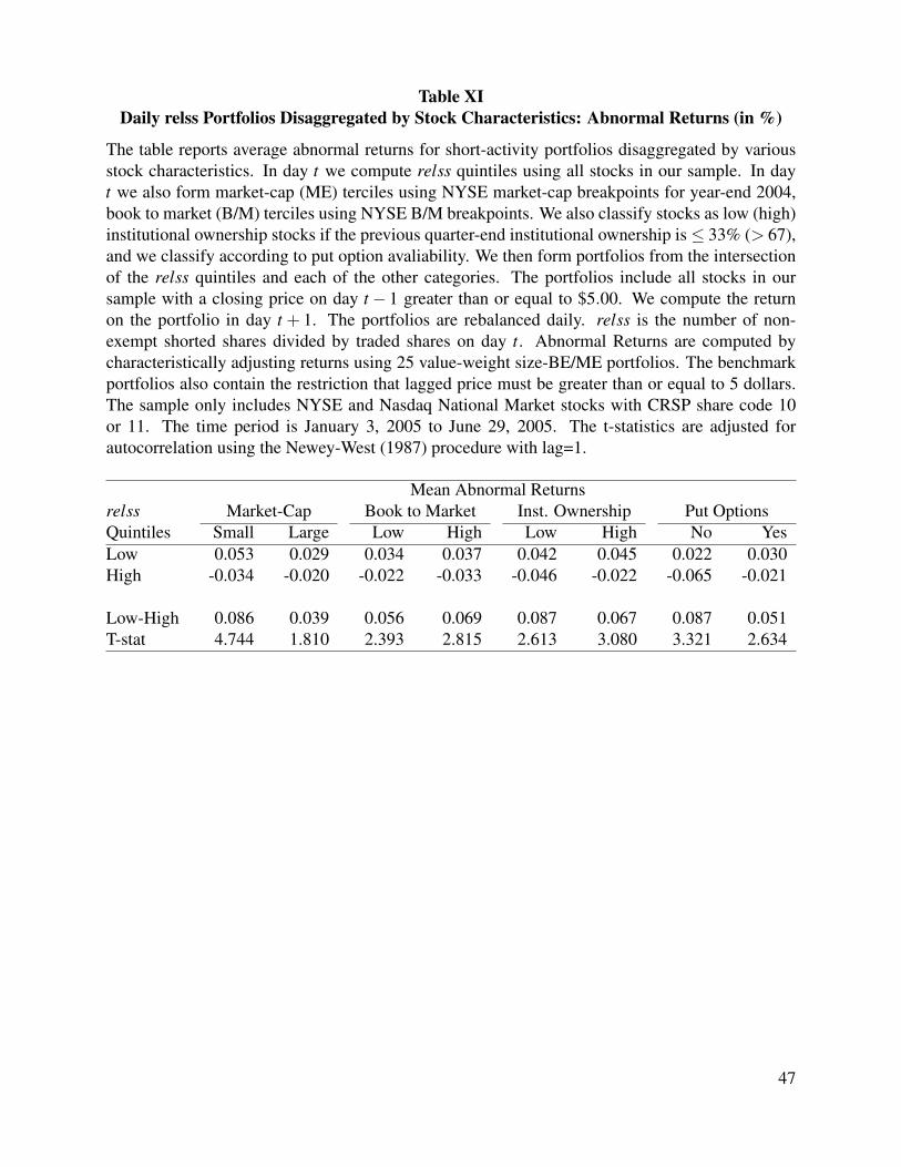
Table XIDaily relss Portfolios Disaggregated by Stock Characteristics: Abnormal Returns (in %)

The table reports average abnormal returns for short-activity portfolios disaggregated by variousstock characteristics. In day t we compute relss quintiles using all stocks in our sample. In dayt we also form market-cap (ME) terciles using NYSE market-cap breakpoints for year-end 2004,book to market (B/M) terciles using NYSE B/M breakpoints. We also classify stocks as low (high)institutional ownership stocks if the previous quarter-end institutional ownership is ≤ 33% (> 67),and we classify according to put option avaliability. We then form portfolios from the intersectionof the relss quintiles and each of the other categories. The portfolios include all stocks in oursample with a closing price on day t− 1 greater than or equal to $5.00. We compute the returnon the portfolio in day t + 1. The portfolios are rebalanced daily. relss is the number of non-exempt shorted shares divided by traded shares on day t. Abnormal Returns are computed bycharacteristically adjusting returns using 25 value-weight size-BE/ME portfolios. The benchmarkportfolios also contain the restriction that lagged price must be greater than or equal to 5 dollars.The sample only includes NYSE and Nasdaq National Market stocks with CRSP share code 10or 11. The time period is January 3, 2005 to June 29, 2005. The t-statistics are adjusted forautocorrelation using the Newey-West (1987) procedure with lag=1.

Mean Abnormal Returnsrelss Market-Cap Book to Market Inst. Ownership Put OptionsQuintiles Small Large Low High Low High No YesLow 0.053 0.029 0.034 0.037 0.042 0.045 0.022 0.030High -0.034 -0.020 -0.022 -0.033 -0.046 -0.022 -0.065 -0.021

Low-High 0.086 0.039 0.056 0.069 0.087 0.067 0.087 0.051T-stat 4.744 1.810 2.393 2.815 2.613 3.080 3.321 2.634

47

Table XIIRobustness Test: Archipelago Short-selling

We regress daily stock level short-selling activity on Archipelago (arelsst ) on past returns and daily stock level futurereturns (rt+1) on arelsst in Panels A and B. In panel C we form value-weight arelss quintile portfolios using NasdaqNational Market stocks. Abnormal Returns are computed by characteristically adjusting returns using 25 equal weightsize-BE/ME portfolios. arelsst is the number of shorted shares on Archipelago divided by all traded shares on day tfor a given stock. r−5,−1 is the return from the closing price on day t−6 to the closing price on day t−1. low (high)is a dummy that equals one if a stock is in the lowest (highest) relsst quintile for Nasdaq stocks. loser (winner) is adummy that equals one if a stock is in the lowest (highest) r−5,−1 quintile for Nasdaq stocks. ME is the market-capfrom the previous month end. B/M is lagged book to market equity as defined in Fama and French (1993).The sampleonly includes Nasdaq National Market stocks with CRSP share code 10 or 11 and lagged price≥ 5. The regressions inPanel A include day and stock dummies, and the standard errors take into account clustering by date. The regressionsin Panel B include day dummies, and the standard errors take into account clustering by calendar date. The time periodis January 3, 2005 to December 30, 2005. T-statistics are in parenthesis. The intercept is estimated but not reported.

Panel A: Dependent Variable = arelsstr−5,−1 0.036 0.026

(18.17) (13.48)log(tv−5,−1) 0.001 0.001 0.001 0.001

(6.16) (5.49) (6.01) (5.51)loser -0.003 -0.003

(9.72) (8.47)winner 0.004 0.003

(13.95) (8.91)relsst−1 0.226 0.225

(58.38) (58.34)R2 0.19 0.23 0.19 0.23Stock Fixed Effects Yes Yes Yes YesDay Fixed Effects Yes Yes Yes Yes

Panel B: Dependent Variable = rt+1arelss -0.233 -0.215

(3.08) (2.82)r−5,−1 -0.008

(4.46)low 0.031 0.028

(0.91) (0.83)high -0.027 -0.024

(2.43) (2.20)loser 0.059

(3.00)winner -0.059

(3.70)Control Variables rt , log(ME), and log(B/M)Day Fixed Effects Yes Yes Yes Yes

Panel C: Value-weight relss portfolios (Abnormal Retrns)Low 2 3 4 High Low-High

Mean 0.056 0.028 -0.027 -0.034 -0.022 0.078T-stat 2.563 1.551 -1.122 -1.428 -1.278 2.716

48

Table XIIIRobustness Test: Pre and Post Reg SHO

We regress relsst on past returns and future returns (rt+1) on relsst . in Panels A and B. We split the data into sub-samples based on whether it is pre (January 3, 2006 to April 30, 2006) or post (May 2, 2006 to December 30, 2006)Reg SHO. relsst is the number of shorted shares divided by all traded shares on day t for a given stock. r−5,−1 isthe return from t− 5 to t− 1. pilot is a dummy that equals one if the stock is part of the Reg SHO pilot program.ME is the market-cap from the previous month end. B/M is lagged book to market equity as defined in Fama andFrench (1993).The sample only includes NYSE and Nasdaq National Market stocks with CRSP share code 10 or 11and lagged price ≥ 5. The regressions in Panel A include day and stock dummies, and the standard errors take intoaccount clustering by calendar date. The regressions in Panel B include day dummies, and the standard errors takeinto account clustering by calendar date. The time period is January 3, 2005 to December 30, 2005. T-statistics are inparenthesis. The intercept is estimated but not reported.

Panel A: Dependent Variable = relsstNYSE NYSE Nasdaq Nasdaq

3-Jan-05 to 2-May-05 to 3-Jan-05 to 2-May-05 to29-Apr-05 30-Dec-05 29-Apr-05 30-Dec-05

r−5,−1 0.378 0.373 0.397 0.374 0.234 0.234 0.202 0.203(31.47) (28.53) (38.68) (33.55) (30.80) (28.50) (31.58) (29.05)

log(tv−5,−1) -0.001 -0.001 -0.006 -0.006 0.002 0.002 0.001 0.001(1.00) (0.99) (8.05) (7.97) (2.13) (2.13) (1.43) (1.43)

r−5,−1 ∗ pilot 0.019 0.093 0.001 -0.006(1.04) (6.41) (0.07) (0.50)

R2 0.26 0.26 0.23 0.23 0.22 0.22 0.18 0.18Stock Fixed Effects Yes Yes Yes Yes Yes Yes Yes YesDay Fixed Effects Yes Yes Yes Yes Yes Yes Yes Yes

Panel B: Dependent Variable = rt+1NYSE NYSE Nasdaq Nasdaq

3-Jan-05 to 2-May-05 to 3-Jan-05 to 2-May-05 to29-Apr-05 30-Dec-05 29-Apr-05 30-Dec-05

relss -0.265 -0.301 -0.108 -0.105 -0.214 -0.225 -0.125 -0.132(3.16) (3.28) (1.84) (1.71) (3.44) (3.48) (3.03) (3.20)

r−5,−1 0.002 0.002 -0.002 -0.002 -0.004 -0.004 -0.009 -0.009(0.31) (0.30) (0.49) (0.49) (1.34) (1.34) (4.41) (4.42)

pilot -0.024 0.005 -0.017 -0.011(0.72) (0.22) (0.31) (0.28)

relss∗ pilot 0.137 -0.013 0.085 0.047(1.31) (0.17) (0.67) (0.58)

Control Variables rt , log(ME), and log(B/M)Day Fixed Effects Yes Yes Yes Yes Yes Yes Yes Yes

49

-0.1%

-0.08%

-0.06%

-0.04%

-0.02%

0%

0.02%

0.04%

0.06%

0.08%

0.1%

0.12%

1 2 3 4 5

Av

era

ge

Ab

no

rma

l R

etu

rns

Holding Period

NYSE Stocks: Daily Low-High relss Portfolio Returns (in %)

Low-High95% Confidence Interval

-0.1%

-0.08%

-0.06%

-0.04%

-0.02%

0%

0.02%

0.04%

0.06%

0.08%

0.1%

0.12%

1 2 3 4 5

Av

era

ge

Ab

no

rma

l R

etu

rns

Holding Period

Nasdaq Stocks: Daily Low-High relss Portfolio Returns (in %)

Low-High95% Confidence Interval

Figure 1: Daily relss Portfolios: Average Abnormal Returns (in Percent)

The figure shows average abnormal returns for short-selling activity portfolios. In day t we com-pute relss quintiles using all stocks in our sample. We then form portfolios using NYSE (Nasdaq)with a closing price on day t − 1 greater than or equal to $5.00. We compute the return on theportfolio in day t +1. We vary the holdin period from one to five trading days. For holding periodsgreater than one trading day we use the overlapping holding period methodology of Jegadeesh andTitman (1993). relss is the number of shorted shares divided by traded shares on day t. AbnormalReturns are computed by characteristically adjusting returns using 25 equal weight size-BE/MEportfolios. The benchmark portfolios also contain the restriction that lagged price must be greaterthan or equal to 5 dollars. The sample only includes NYSE (Nasdaq) stocks with CRSP share code10 or 11. The time period is January 3, 2005 to December 28, 2005. Standard errors are adjustedfor autocorrelation using the Newey-West (1987) procedure with lag=5.

50