Can Labour Regulation Hinder Economic

Performance? Evidence from India*

by

Timothy Besley and

Robin Burgess

London School of Economics

` The Suntory Centre Suntory and Toyota International Centres for Economics and Related Disciplines London School of Economics and Political Science Houghton Street

DEDPS 33 London WC2A 2AE February 2002 Tel.: (020) 7955 6674 * We are grateful to Roli Asthana, Abhijit Banerjee, Rohini Pande, Andrei Shleifer, Michael Smart, Chris Udry and seminar participants at Harvard/MIT, Yale and LSE for useful comments and suggestions. Berta Esteve-Volart, Shira Klien, Silvia Pezzini, Pataporn Sukontamarn and Kamakshya Trivedi provided excellent research assistance. The first draft of the paper was written while Burgess was visiting MIT Economics Department which he wishes to thank for support and encouragement. We thank STICERD for financial support.

Abstract

This paper investigates whether the industrial relations climate in Indian States has affected the pattern of manufacturing growth in the period 1958-92. We show that pro-worker amendments to the Industrial Disputes Act are associated with lowered investment, employment, productivity and output in registered manufacturing. Regulating in a pro-worker direction is also associated with increases in urban poverty. This suggests that attempts to redress the balance of power between capital and labour can end up hurting the poor. Keywords: Indian industrial relations; Industrial Disputes Act; manufacturing growth; pro-worker regulations; urban poverty; capital and labour. JEL Nos.: H0, H1, I3, J5, K2, L5, L6, O2, O4. © the authors. All rights reserved. Short sections of text, not to exceed two paragraphs, may be quoted without explicit permission provided that full credit, including © notice, is given to the source. Contact address: Dr Robin Burgess, STICERD, London School of Economics and Political Science, Houghton Street, London WC2A 2AE. Email: r.burgess@lse.ac.uk .

1 Introduction

One of the key challenges of development economics is to identify policiesthat harm or hinder growth, along with an assessment of their effectivenessin poverty reduction. Traditional views of the growth process put develop-ment of manufacturing at centre stage in the structural change accompany-ing economic development.1 A casual look at the performance of some of themore successful Asian economies after 1960 adds credence to this view. Forexample, between 1960 and 1995, manufacturing as a share of GDP grewfrom 9 percent to 24 percent of GDP in Indonesia, 8 percent to 26 percent inMalaysia and 12.5 percent to 28 percent in Thailand. All of these countrieshad strong overall growth performances and saw significant falls in absolutepoverty.In contrast, the Indian economy did not experience a significant expan-

sion of manufacturing as a share of national income. Manufacturing outputconstituted 13 percent of GDP in 1960 (ahead of the countries listed above)but grew to only 18 percent of GDP by 1995. India’s overall growth over thisperiod was also relatively modest and did not exhibit the extent of decliningabsolute poverty experienced elsewhere in Asia. While this pattern reflectsa complex array of phenomena, a key issue concerns the way in which policychoices can be identified as playing a role.This paper studies the role of labor market regulation in explaining the

performance of Indian manufacturing between 1958 and 1992. There are fourreasons for this focus. First, labor market regulations have frequently beencited in explaining India’s poor growth performance [see, for example, Dollar,Iarossi and Mengitsae 2001, Stern 2001 and Sachs, Varshey and Bajpai 1999].The charge is that granting excessive bargaining power to organized laborblunted investment incentives and gave India a generally unfavorable businessclimate. Second, in the Indian constitution labor regulation is in part underthe control of the states. This means that different parts of India faceddifferent regulatory climates. This gives rise to both time series and cross-sectional variation that can be used to identify its effects. Third, regulationapplies to a specific sector — registered manufacturing — which provides afocus for studying its impact. Fourth, the choice of period is opportune asit extends from the heyday of central planning in the late 1950s to the onsetof liberalization in 1992. Whilst there was some dismantling of planning

1See, for example, Kaldor [1967] for an early forcefull statement of this view.

1

structures during this period manufacturing remained highly protected frominternational competition. This helps us to isolate the impact of domesticpolicies on industrial performance.Between 1958 and 1992 manufacturing grew by 3.3 percent in India as

a whole. This, however, masks significant variations across states. Forexample, West Bengal which was the largest producer of manufactured out-put per capita at the beginning of the period had fallen to seventh in 1992with output per capita falling at an average rate of 1.5 percent per annum.West Bengal was also a state that had the greatest body of pro-worker laborregulation passed in the state legislature. Its performance contrasts withAndhra Pradesh which grew at nearly 6 percent per year over the same pe-riod but which experienced anti-worker labor regulation. Here, we developan econometric analysis of whether the patterns of regulation can accountfor the cross-state variation in patterns of manufacturing performance overtime. The analysis is consistent with the view that pro-worker labor reg-ulation resulted in lower growth of manufacturing output, investment andemployment. Regulating in a pro-worker direction also resulted in lowerrates of poverty reduction over the period.Our data on labor regulation come from looking at state amendments

to the Industrial Disputes Act of 1947. While the act was passed at thecentral level, state governments were given the right to amend it under theIndian Constitution. We read the text of each amendment (121 in all) andclassified each as pro-worker, pro-employer or neutral. This gave a sense ofwhether workers or employers benefited or whether the legislation had noappreciable impact on either group. The results are interpreted through thelens of a simple two-sector model of incomplete contracts where firms investin capital ahead of bargaining with labor over the surplus.The paper illuminates long-standing debates about the role of the state

in promoting or hindering economic development. While there is now anabundance of cross-country evidence on determinants of growth, relativelylittle of this identifies robust relationships with policy regimes. Moreover,there is the inevitable difficulty of identifying the true sources of variation ina predominantly cross-sectional context. The relatively long time period (35years) and the fact that so much of the policy environment is common to theIndian states makes it an ideal testing ground for the effects of regulation onoutput and welfare.The remainder of the paper is organized as follows. In the next section,

we review the literature on regulation and economic performance. In section

2

three we trace the evolution of labor market regulation in India, detail howwe capture the direction of regulatory change and examine how economicperformance has varied across different states. In section four, we set outa simple two sector model in which affecting the bargaining power of laboraffects the pattern of employment and capital accumulation in an economy.The model is based on incomplete contracts between labor and capitalists.Section five contains the empirical analysis of the effect of labor regulation onmanufacturing performance. Section six turns to the welfare consequencesof regulation in terms of poverty reduction and section seven concludes.

2 Related Literature

There is a significant literature on cross-country growth, much of which hastried to study how policies impact on economic performance [see Barro, 1997].Few simple and definitive lessons about the role of the state have emergedfrom this. In early cross-country growth work, government activism was of-ten proxied crudely by some measure of the size of the state [see Temple, 1999for a review]. However, the results tend not to be robust and conceptually,it is not clear whether this captures anything interesting from a theoreticalpoint of view. Hall and Jones [1999] provides one of the most compellingefforts at identifying the effect of government on growth by developing an in-dex of social infrastructure reflecting a broad range of government activitiessuch as contract enforcement, bureaucratic quality and government repudia-tion of contracts. In OLS and IV specifications, they find that good socialinfrastructure is positively related to growth.Looking at policies directly is notoriously difficult given that the details of

government intervention vary strongly across countries. An important andinnovative contribution in this vein is the recent paper by Djankov et al [2002]which looks at regulations governing the start of businesses in a cross-sectionof 85 countries.2 This is a potentially important way of measuring regulatoryseverity cross-sectionally. They find that countries with higher regulationof entry have less impressive performance across an array of social, politicaland economic indicators. Of particular note in relation to this study, theyfind that greater regulation expands the size of the unofficial economy. Theyargue that this is in line with a public choice view of regulation as being put

2In the context of our study it is interesting to note that India is close to average inthis dimension. Moreover, it is ranked above Indonesia and Japan.

3

in place by officials or insiders intent on extracting rents (see, for example,Stigler [1971], De Soto [1989], and Shleifer and Vishny, [1998]).Our focus is on labor market regulations. This is related to studies

of how economic performance has varied among OECD economies whichhave frequently cited labor market institutions as a determinant of economicperformance [see Freeman, 1988; Blanchard, 2000; Lindbeck and Snower,2001]. Blanchard and Wolfers [2000] which builds on Nickell [1997] considerhow observable shocks interact with institutions in explaining the evolutionof European unemployment. While institutions are fixed cross-sectionally,interacting them with time-varying regressors allows their dynamic effects tobe considered. They conclude that interacting shocks and institutions doesa good job at accounting for the variation in unemployment across Europe.Nickell and Layard [2000] argue that, for European countries, labor marketinstitutions such as unions and social security systems are important driversof economic performance with strict labor market regulations, employmentprotection and minimum wages playing a lesser role.This work is also related to that which looks at whether the political

complexion of governments changes economic performance [see, for example,Alvarez, Garrett and Lange, 1991]. This literature looks, for example, atwhether having left leaning governments in office lowers growth. We showthat the propensity of governments in India to pass labor regulations is afunction of political control and hence that they provide a mechanism bywhich political history has a lasting effect on economic performance.The strategy of state led industrialization which India adopted at In-

dependence has meant that government policies have taken center stage intrying to explain manufacturing performance up to the onset of liberalizationin 1992 [see Mookherjee, 1997]. Bhagwati and Desai [1970] discuss how therequirement to obtain a license to set up a new unit or expand productionserved as a barrier to entry and limited competition.3 The advisability ofclosing off Indian industry behind a range of tariff and non-tariff barriers asa means of promoting infant industries has also been the subject of heateddebate. Singh [1964] and Bhagwati and Srinivasan [1975] were early critics inparticular as regards the presumption of export pessimism. Bhagwati [1998]points to the choice of an import substitution strategy over export promotionas being a major reason as to why India did not experience a development

3This led to a ‘license raj’ where the benefits of industrialization became concentratedin the hands of a few major firms.

4

“miracle” of the type seen in various East Asian countries [see World Bank,1993].Central planning and trade protection, however, have limited scope in ex-

plaining cross-state variation in manufacturing performance over time. Herenotions of ‘business’ or ‘investment’ climate, which in part reflect state con-trolled policies, take center stage. And these factors became increasinglyimportant over the 1958-1992 period as firms and capital become increas-ingly mobile.4 Stern [2001] points to improvement of the investment climateas being key to increasing productivity and reducing poverty and identifiesreform of India’s cumbersome labor regulations as a priority. Sachs, Varsheyand Bajpai [1999] echo this sentiment by pointing to restrictive regulationson labor redundancy as being a key reason as to why India has done poorlyin terms of export performance. Using a cross-sectional survey of about onethousand manufacturing establishments drawn from ten Indian states Dol-lar, Iarossi and Mengitsae [2001] show that productivity is forty-four percentlower in states judged by managers to have poor business climates. Theythen break apart investment climate. Entrepreneurs were asked how muchof their labor force they would lay off if there was greater labor market flex-ibility to capture the ‘cost’ of labor regulation.5 This factor alongside otherswas found to be important in explaining cross-state differences in productiv-ity.6 Fallon [1987] and Fallon and Lucas [1993] argue that strengthening jobsecurity regulations through central government amendment of the Indus-trial Disputes Act in 1976 and 1982 was associated with a reduction in labordemand in firms covered by the regulation but not in small firms uncoveredby job security regulations. The stringency of employment protection reg-ulation has thus been used to explain the phenomena of jobless growth inindustry in the 1980s whereby industrial output growth was accompanied bystagnation in employment [see Bhalotra, 1998].

4Though radical liberalization only took place from 1992 onwards steps to relax anddismantle central controls and regulations were being undertaken from the early 1970s [seeMookherjee, 1997].

5The average figure was 16-17 percent.6Other factors included power reliability, visits from government regulators, custom

clearance delays and internet connectivity.

5

3 Institutional Background and Data

Our aim is to look at whether the direction of labor regulation affects eco-nomic performance across Indian states. As we note above, there is con-siderable variation in economic performance which could have a variety ofexplanations. The particular focus on labor regulation in this paper is moti-vated by the observation that states retain a considerable degree of autonomyin determining this unlike other forms of regulation. In addition, it is regu-lation which targets a particular sector — registered manufacturing which iscomprised of firms with more than ten employees with power or more thantwenty employees without.7

3.1 Labor Regulation in India since Independence

Since Independence India has been a federal democracy. The Indian Con-stitution of 1949 divides legislative powers into three lists — the Union List,the State List and the Concurrent List. Central and state governments aresovereign as regards making laws relating to matters in the Union and StateLists, whereas both central and state governments can make law relating tomatters in the Concurrent List. While the Constitution did provide the stateswith some jurisdiction over industrial development,8 these powers could beoverridden by central government powers. Specifically Entries 7, 52 and 54of the Union List give the central government jurisdiction over defense in-dustries and over other industries and mines when this is deemed to be inthe ‘public interest’. This public interest clause was invoked in the Industries(Regulation and Development) Act of 1951 which effectively granted centralgovernment control over all key industries in India.The situation as regards industrial labor was different. Matters relating

to trade unions and industrial and labor disputes fall under the ConcurrentList (Entry No. 22). This implies that both central and state governmentsare empowered to introduce legislation with respect to these matters. The

7This definition comes from the definition of a factory in the Factories Act of 1948. Allfirms which fit this description have to register with Industrial Inspectorates in each stateand are surveyed on an annual basis by the Annual Survey of Industries. This impliesthat we have detailed information on the functioning and performance of the registeredmanufacturing sector across states and time.

8Entries 23, 24 and 27 of the State List authorize the states to regulate mines andmineral development, industries and the production, supply and distribution of goods.

6

key piece of central legislation relating to industrial disputes is the Indus-trial Disputes Act of 1947 which sets out the conciliation, arbitration andadjudication procedures to be followed in the case of an industrial dispute.This Act has been extensively amended by state governments during thepost-Independence period. It is these amendments that we use to studythe impact of labor market regulation on manufacturing performance andpoverty.The Industrial Disputes Act was designed to offer workers in the orga-

nized sector some protection against exploitation by employers. This was incontrast with labor legislation introduced prior to World War I which wasdesigned to limit labor rights and to protect the commercial interests of theBritish.9 This Act, which is in forty sections, specifies the powers of gov-ernment, courts and tribunals, unions and workers and the exact proceduresthat have to be followed in resolving industrial disputes.10 It defines thebargaining positions of the different parties involved in an industrial dispute.As noted above, state legislatures have the power to amend this act.

3.2 Coding Legislative Changes

Our effort to measure the direction of policy in a state began by readingthe text of all state level amendments to the Industrial Disputes Act of 1947from Malik [1997]. Our reading of the individual amendments lead us to codeeach one as either being neutral, pro- or anti-worker. While this method

9Political reforms introduced after the war and the fact that India had joined theInternational Labor Organization in 1919 provided some impetus to protect the interestsof labor culminating in the Trade Union Act of 1926. Major strikes in 1928 involvingthe cotton textile industry of Bombay, Tata Iron and steel workers and railway workers,however, made it transparent that there was no effective machinery for the settlement ofindustrial disputes. (See Kannappan [1959] for an analysis of the Tata Steel strike.) TheTrade Disputes Act passed in 1929 which required unions to give 14 days notice prior tostrikes in public utility concerns and which prohibited strikes which might cause severehardships to the public and the Bombay Industrial Disputes Act passed in 1938 served asprecursors to the Industrial Disputes Act of 1947.10Sections are arranged within seven chapters which cover (I) definitions; (II) authorities

under this Act, notice of change and reference of certain individual disputes to grievancesettlement authorities; (III) reference of disputes to Boards, Courts or Tribunals; (IV)procedures, powers and duties of authorities; (V) strikes and lockouts, lay-off and re-trenchment, special provisions relating to lay-off, retrenchment and closure in certainestablishments, unfair labour practices; (VI) penalties and (VII) miscellaneous [see Malik,1997].

7

of classification required a number of judgement calls, we found surprisinglyfew cases of uncertainty.11 We coded each pro-worker amendment as a one,each neutral amendment as a zero, and each anti-worker amendment as aminus one.It is useful to give a couple of examples of this procedure. A sample pro-

employer reform is from Andhra Pradesh in 1987. Our synopsis is: “If inthe opinion of the state government it is necessary or expedient for securingthe public safety of the maintenance of public order or services or suppliesessential to the life of the community or for maintaining employment orindustrial peace in the industrial establishment it may issue an order which(i) requires employers and workers to observe the terms and conditions of anorder and (ii) prohibits strikes and lockouts in connection with any industrialdispute.” This amendment gets a code of minus one in our data. A samplepro-worker reform is from West Bengal in 1980 where our synopsis is: “Therules for lay-off, retrenchment and closure may according to the discretion ofthe state government be applied to industrial establishments which employmore than 50 workers. Under the central act, these rules only apply toestablishments which employ more than 300 workers.” This gets coded as aplus one in our data.Having obtained the direction of amendments in any given year, we cu-

mulated the scores over time to give a quantitative picture of the regulatoryenvironment as evolved over time. This is our basic regulatory measureused below. In years in which there were multiple amendments, we use anindicator of the general direction of change. So, for example, if there werefour pro-worker amendments in a given state and year, we would only codethis as plus one rather than plus four.This method of analysis divides the states into “treatment” and “con-

trol” groups. The latter are states that do not experience any amendmentactivity in a pro-worker or pro-employer direction over the 1958-1992 pe-riod. There are six of these: Assam, Bihar, Haryana, Jammu & Kashmir,Punjab and Uttar Pradesh. Among those that have passed amendments,our method classifies six states Andhra Pradesh, Karnataka, Kerala, MadhyaPradesh, Rajasthan and Tamil Nadu as “pro-employer”. This leaves four“pro-worker” states: Gujarat, Maharastra, Orissa and West Bengal. Figure

11Summaries of all amendments and their coding is available athttp://econ.lse.ac.uk/staff/rburgess/#wps.

8

1 graphs the history of the regulatory structure across states over the periodin question. For the most part, changes are monotonic although states movein different directions.For later reference, it is important to see that the Indian experience gives

important sources of both time-series and cross-sectional variation in regula-tion. Finding comparable variation while being able to control for commoninstitutions is problematic even in OECD countries. The empirical analysiswill exploit the time-series dimension of change and will incorporate statefixed effects in the analysis.

3.3 Background Facts

Overall, non-agricultural output per capita in India accounts for 66 percentof total output. Among non-agricultural output, on average manufacturingis about 13 percent of total state output of which 9 percent is in registeredmanufacturing. The share of registered manufacturing in total manufactur-ing has increased over time from 50 percent to 65 percent over the period inquestion.Figures 2 and 3 give an idea of how economic performance in registered

manufacturing varies by Indian states. Figure 2 looks at registered manu-facturing output per capita and Figure 3 at employment in registered man-ufacturing over our data period for each of the sixteen states in our sample.Certain states: Andhra Pradesh, Gujarat, Karnataka, Tamil Nadu and Ma-harashtra show striking growth, while states like Assam, Jammu and Kashmirand West Bengal display relative stagnation (albeit from very different baselevels). Note that we have both pro-worker and pro-employer states amongthe fast growers.Table 1 breaks out certain state indicators by the type of regulatory

stance of the state. These show that the pro-worker states on average hadhigh registered manufacturing output in 1960 relative to control states andpro-employer states. By 1990, there is no statistically significant differencebetween pro-worker and pro-employer states. Moreover, the average regis-tered manufacturing output in the pro-employer states has overtaken that inthe control states. This pattern is less pronounced when looking at over-all output per capita. Other state characteristics such as total taxes percapita, development expenditure per capita, installed electricity per capitaand literacy show no significant difference between treatment and controlstates.

9

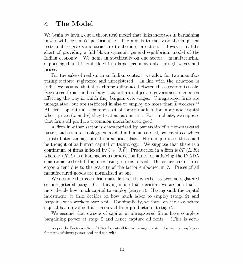
4 The Model

We begin by laying out a theoretical model that links increases in bargainingpower with economic performance. The aim is to motivate the empiricaltests and to give some structure to the interpretation. However, it fallsshort of providing a full blown dynamic general equilibrium model of theIndian economy. We home in specifically on one sector — manufacturing,supposing that it is embedded in a larger economy only through wages andprices.For the sake of realism in an Indian context, we allow for two manufac-

turing sectors: registered and unregistered. In line with the situation inIndia, we assume that the defining difference between these sectors is scale.Registered firms can be of any size, but are subject to government regulationaffecting the way in which they bargain over wages. Unregistered firms areunregulated, but are restricted in size to employ no more than L workers.12

All firms operate in a common set of factor markets for labor and capitalwhose prices (w and r) they treat as parametric. For simplicity, we supposethat firms all produce a common manufactured good.A firm in either sector is characterized by ownership of a non-marketed

factor, such as a technology embedded in human capital, ownership of whichis distributed among an entrepreneurial class. For our purposes this couldbe thought of as human capital or technology. We suppose that there is acontinuum of firms indexed by θ ∈ £θ, θ¤. Production in a firm is θF (L,K)where F (K,L) is a homogeneous production function satisfying the INADAconditions and exhibiting decreasing returns to scale. Hence, owners of firmsenjoy a rent due to the scarcity of the factor embodied in θ. Prices of allmanufactured goods are normalized at one.We assume that each firm must first decide whether to become registered

or unregistered (stage 0). Having made that decision, we assume that itmust decide how much capital to employ (stage 1). Having sunk the capitalinvestment, it then decides on how much labor to employ (stage 2) andbargains with workers over rents. For simplicity, we focus on the case wherecapital has no value if it is removed from production at stage 2.We assume that owners of capital in unregistered firms have complete

bargaining power at stage 2 and hence capture all rents. (This is actu-

12As per the Factories Act of 1948 the cut-off for becoming registered is twenty employeesfor firms without power and and ten with.

10

ally stronger than we need as we explain below.) The firm then behavesjust like a standard firm where labor and capital hiring decisions equate themarginal product to the price. The only restriction faced by an unregisteredfirm is that the number of workers hired at stage 2 cannot exceed L. LetπU¡r, w, θ;L

¢be the conditional profit function in the unregistered sector.13

Turning now to the registered manufacturing sector, we assume there isa well-defined pool of “inside” workers with whom the firm bargains if itregisters. (In reality, it is best to think of this as a union.) We assumethat contracts are incomplete along the lines described in Grout [1984] — anycontracts negotiated at the time of the capital accumulation decision are sub-ject to renegotiation ex post, creating a hold-up problem.14 Following Grout[1984], we use a generalized Nash bargaining solution with bargaining powerof firm owners being represented by α ∈ [0, 1]. Using his results, the equi-librium payoff to a firm owner in the unregistered sector is απR

¡rα, w, θ

¢.15

The bargaining power of the firm enters now in two places — affecting directlythe share of the rent that the firm owner receives and the “price” of installedcapital. Ex post bargaining ensures that labor is allocated efficiently at

13Formally, this is defined as:

πU¡w, r, θ, L

¢= argmax

©f (L,K)− rK −wL : L ≤ Lª

14For a detailed macro-economic analysis of an economy with hold-up issues, see Ca-ballero and Hammour [1998].15The rents in the firm are distributed as:

argmaxL,T

θF (K,L)−wL− Tα T(1−α)

where the threat point is assumed to be zero payoffs all round. The capital accumulationdecision solves:

αθFK (K,L) = r.

In this case it is as if the profit function being maximized is,

πR³ rα, w, θ

´= argmax

nθF (K,L)− r

αK −wL

o

11

price w. However, because of the hold-up problem, more bargaining powerfor workers raises the cost of capital to r/α > r. Thus less capital is installedand less labor is also employed.16

Firms can choose one of three states: inactivity, being registered or un-registered. A firm is inactive if it would make a loss no matter which sectorit operated in. It is now straightforward to determine the equilibrium size ofthe registered sector.

Proposition 1 There are three possible cases:1. For high enough L and low enough α all active firms are unregistered2. For low enough L and high enough α all active firms are registered.3. Otherwise, there exists a critical value bθ ¡α, L¢ which is decreasing in

α and increasing in L such that all firms with θ ≥ bθ ¡α, L¢ choose to register.In this case, an increase in the bargaining power of labor reduces the size ofthe registered manufacturing sector and increases the size of the unregisteredmanufacturing sector (other things being equal).

Thus unless we are at one of the boundary cases (which is not empiricallythe case in our data), then we expect the size of the registered manufacturingsector to be larger in states that give greater bargaining power to owners offirms. Total labor and capital used in the registered sector (assuming an

interior solution for bθ ¡α, L¢) areLR =

Z θ

bθ(α,L) L³ rα, w, z

´dz and KR =

Z θ

bθ(α,L)K³ rα, w, z

´dz. (1)

Using these, it is straightforward to show the following empirical implicationof our model:

Proposition 2 An increase in the bargaining power of labor (i) reduces out-put, capital formation and employment in the registered manufacturing sec-tor; (ii) increases output in the unregistered manufacturing sector and (iii)reduces overall manufacturing output.

16The model has one-sided investment, i.e., by owners of capital. If workers were alsoallowed to invest in firm specific human capital, then the effect of increasing the bargainingpower of workers on investment would depend upon the relative importance of firms’ andworkers’ investments in the production process.

12

The third part of Proposition 2 says that overall output in manufacturingis lower if workers in registered firms have greater bargaining power. Thisstems from the fact that a firm will chose to register only if it will produce asignificantly higher amount of output to compensate for the loss in bargainingpower. Hence, on the margin, an increase in the fraction of firms that donot register reduces manufacturing output.Earnings of workers in the registered manufacturing sector have two com-

ponents: wage labor earnings and rents captured in the bargaining process.In our data, we have only measures of total earnings of workers which cap-tures both components. Thus, absent general equilibrium effects on wages, itis the rental component of earnings that responds to labor market regulation.In terms of the theoretical model, this is:

(1− α)

Z θ

bθ(α,L) πR³ rα, w; z

´dz.

There are three effects of increasing worker bargaining power which can goin different directions. First, a fall in α increases the effective cost of capitalby exacerbating the hold-up problem. This lowers total rents. Through thiseffect it also reduces the size of the registered sector on the margin, and hencealso lowers rents in the registered sector. These are both bad for workers.However, there is a first order effect that increasing worker bargaining powerincreases the share of any given available rents which makes workers as awhole better off.17 In general, we expect there to be a rent maximizing valueof α strictly below one. Hence workers would not want to see all bargainingpower going to them as it reduces incentives for capital accumulation. In aneighborhood of the optimal α, there would be no effect of increasing laborpower on total labor earnings (barring general equilibrium effects on wages).The model does not embed the decision within a federal system like In-

dia’s. In reality entrepreneurs may be able to choose between registered orunregistered sectors in a number of states. As we argued above, α is likely tobe state dependent depending on the regulatory structure in place governingindustrial relations. We view an increase in our regulatory measure as akinto a fall in α. We might also expect other features of states (such as their

17This result generalizes to allowing workers to share in the rents in unregistered man-ufacturing provided that their share of the rents in that sector is lower than their share inthe registered sector.

13

infrastructure to govern the allocation decision). In principle, all registeredfirms would want, according to the model, to migrate to the state with thehighest α. In reality, we might expect θ to contain some kind of state specificcomponent which gives a potential entrepreneur a comparative advantage inremaining within a state. This could be due to cultural factors such asspeaking local languages or access to supplier networks etc. However, therewill still be a possible margin of substitution across states which can resultin firms choosing to set-up in other jurisdictions.

5 Empirical Method

The model yields predictions that can be tested empirically. For state sand time t, there are parameters (rt, wst,αst) which vary (along with otherimportant factors that makes states attractive or unattractive as a place to dobusiness). We will suppose that the industrial relations climate is capturedby our regulatory measure discussed above which varies both at the statelevel and over time.We have direct measures of a number of the variables from the theory:

output in the registered and unregistered manufacturing sectors. We alsohave measures of employment and fixed capital for the registered sector. Forthe former we have a variety of different measures from two different datasources. In addition, we use number of registered “factories” in a stateas a crude measure of investment. We also use data on value added perworker. To get a handle on worker rents, we also have three sources of dataon remuneration of workers in the registered manufacturing.We run panel data regressions of the form:

yst = αs + βt + λyst−1 + µrst + ξxst + εst

where yst is a (logged) outcome variable, rst is the regulatory measure, xst arethe exogenous variables of interest that explain the outcomes, αs is a statefixed effect and βt is a year effect. We allow for robust standard errors.We expect differences in climate and culture to be picked up in the fixed

effects along with heterogeneous initial conditions. We have experimentedwith a number of different specifications and sets of control variables. Inthe tables below, we use development expenditure per capita and installedelectricity capacity as our controls (the xst). The presence of a lagged

14

dependent variable reflects the reasonable supposition that the patterns inthe data are affected by slow moving capital stocks reflecting long rangedecisions with relative immobility of capital ex post. It allows us to interpretthe parameters on the other exogenous variables as growth effects.18

In the case of registered manufacturing output, employment and capital,we expect a more pro-worker regulatory regime to be associated with lowergrowth. While overall output in manufacturing will be lower, we expect it tobe higher in the unregistered sector. As well as focusing on outcome variablesthat the theory predicts are affected, it is also useful to check that laborregulation in the registered manufacturing sector does not affect outcomesin other sectors where we expect it not to bite. Thus, we also estimate themodel with agricultural output as an outcome measure.Given our rather crude quantification of the regulatory regime, it will

be important to check robustness to alternative measures. We will attemptto differentiate pro-worker or pro-employer regulation from general activism.Hence, we will introduce the total number amendments to the IndustrialRelations Act as a regressor, ignoring the direction of change.A further concern is that there is some common omitted factor which is

driving both regulation and economic performance. Ideally, this would bedealt with by instrumenting regulation. However, it is hard to find a factorthat affects regulation, but which will not affect economic performance di-rectly. One intermediate way into this is to recognize that regulation (likemany policies) is an intensely political activity. The fact that the amend-ments to the Industrial Disputes Act that we code in our data have to bepassed in the state legislatures guarantees this is the case. We thus con-struct “political histories” for each state by looking at patterns of historicalpolitical control by looking at episodes of majority control in the legislature.During our data, there are five political groupings that control state legisla-tures — hard left parties, the Congress party, Hindu parties, Janata partiesand regional parties. In each year, we created a dummy variable equal toone if one of these groups controls the legislature. To create a history vari-

18 The presence of a lagged dependent variable in a panel with fixed effects raises theusual issue of bias. In this instance, the longish time horizon, probably means that thisis not hugely important. In each of our models, we test for autocorrelation in the errorsusing a test that is robust to the existence of a lagged dependent variable. Since inall cases, we find none, we proceeded without making any allowance for this. We alsoperformed the test for stationarity in panel data suggested by Madalla and Wu [1999]which seemed to suggest no difficulty with assuming stationarity.

15

able, we cumulate this pattern of political control. So for example, if a statehad a Congress majority three times in the past this variable would take onthe value 3 in that state ever after. We then show that regulation is highlycorrelated with this pattern of control. We then introduce them directlyinto the xst vector above as regressors which might be picking a whole arrayof omitted policies affecting development of registered manufacturing.

6 Results

This section gives our main empirical results on the empirical links betweenlabor regulation and development of manufacturing in India. We begin bylooking at measures of sectoral output per capita at the state level. Wethen focus more on outcomes specific to the registered manufacturing sector— employment, labor earnings, fixed capital investment, numbers of factoriesand efficiency. We then discuss a number of robustness checks includingdifferent ways of measuring regulation. Finally, we consider the possibilitythat labor regulation could be proxying for other policy choices.

6.1 Basic Results

We first look at measures of output per capita in Table 2. Total state outputper capita is in column (1). The data here suggests no correlation betweenoutput and the labor regulation regime. A negative correlation is apparentin column (2) which looks only at non-agricultural output per capita. Thereis no good reason to expect any correlation with agricultural output which isconfirmed in column (3). This result is reassuring since these regulations haveno direct effect on the agricultural sector.19 Column (4) shows that the pointestimate becomes larger and more significant when looking at manufacturingoutput. This is consistent with the final prediction of Proposition 2.In column (5), we look only at registered manufacturing output and now

find an even larger and more statistically significant effect. Looking at othercoefficients, there is some evidence that the stock of installed electricity ca-pacity is positively correlated with registered manufacturing. Turning tounregistered manufacturing, we get the opposite sign — that high levels of

19This suggests that general equilibrium effects which feedback on to the agriculturalsector have not been important. Given the size of the registered manufacturing sector,this is not too surprising.

16

pro-worker labor regulation encourages unregistered manufacturing. Theseresults make sense as the labor regulations we are looking at apply to firmsin the registered manufacturing but not to those in the unregistered manu-facturing sector. Our findings are thus directly in line with the predictionof Proposition 1.The growth effect of labor regulation in column (5) of Table 2 goes some

way towards explaining the differences in growth rates across the Indianstates. To illustrate this, consider Andhra Pradesh, which grew at 6 percentper annum between 1958 and 1992. Our estimate predicts that it would havegrown at 4.1 percent had it not passed pro-employer reforms. West Bengal,whose registered manufacturing output per capita declined at 1.5 percentper annum over the data period would have grown at 2.2 percent, accordingto the point estimate in column (5), had it not legislated in a pro-workerdirection. Thus we can explain more than two thirds of the difference intheir growth rates.We now look at a number of performance measures within the registered

manufacturing sector. Table 3 considers four employment measures takenfrom two different sources. The data in columns (1), (2) and (3) comefrom an industrial census — the Annual Survey of Industries — while that incolumn (4) which is based on returns from registered manufacturing firmscomes from the Indian Labor Yearbook.20 The first variable (number ofemployees) in column (1) gives the broadest definition of employment andincludes (“blue collar”) workers as well as those in supervisory or managerialpositions. Workers in column (2) are therefore a subset of employees. Themandays variable in column (3) is defined as the total number of days workedin a year and is a measure of gross labor input employed in the sector. Dailyemployment in column (4) defined as total worker attendances over a yeardivided by the total number of days worked by the factory has the advantagethat it is a measure of the intensity of labor usage. However, there issignificant variation in the fraction of firms furnishing a return which makes

20All firms in the registered manufacturing sector (i.e. those with ten or more employeeswith power or with twenty or more employees without) are under the Factories Act of1948 required to submit returns to State Chief Inspectors of Factories. Compliance withthis requirement is variable which introduces a bias into the Indian Labour Yearbookfigures. In contrast the Annual Survey of Industries covers all the firms in the registeredmanufacturing sector — those with more 100 employees are completely enumerated whereasfirms with less than 100 employees are captured via stratified sampling. This implies thatASI data is likely to more reliable, however, we include both sources as a robustness check.

17

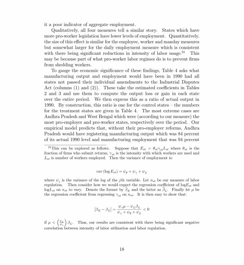
it a poor indicator of aggregate employment.Qualitatively, all four measures tell a similar story. States which have

more pro-worker legislation have lower levels of employment. Quantitatively,the size of this effect is similar for the employee, worker and manday measuresbut somewhat larger for the daily employment measure which is consistentwith there being significant reductions in intensity of labor usage.21 Thismay be because part of what pro-worker labor regimes do is to prevent firmsfrom shedding workers.To gauge the economic significance of these findings, Table 4 asks what

manufacturing output and employment would have been in 1990 had allstates not passed their individual amendments to the Industrial DisputesAct (columns (1) and (2)). These take the estimated coefficients in Tables2 and 3 and use them to compute the output loss or gain in each stateover the entire period. We then express this as a ratio of actual output in1990. By construction, this ratio is one for the control states — the numbersfor the treatment states are given in Table 4. The most extreme cases areAndhra Pradesh and West Bengal which were (according to our measure) themost pro-employer and pro-worker states, respectively over the period. Ourempirical model predicts that, without their pro-employer reforms, AndhraPradesh would have registering manufacturing output which was 84 percentof its actual 1990 level and manufacturing employment that was 94 percent

21This can be explored as follows. Suppose that Est = θstγstLst where θst is thefraction of firms who submit returns, γst is the intensity with which workers are used andLst is number of workers employed. Then the variance of employment is:

var (logEst) = ψθ + ψγ + ψL

where ψj is the variance of the log of the jth variable. Let nst be our measure of laborregulation. Then consider how we would expect the regression coefficient of logEst andlogLst on nst to vary. Denote the former by bβE and the latter as bβL. Finally let µ bethe regression coefficient from regressing γst on nst. It is then easy to show that:

[βE − βL] =ψγµ− ψLβLψγ + ψθ + ψL

< 0

if µ <³ψLψγ

´βL. Thus, our results are consistent with there being significant negative

correlation between intensity of labor utilization and labor regulation.

18

of its 1990 level. Had West Bengal not passed any pro-worker amendmentsit would have enjoyed a registered manufacturing output that was 14 percenthigher than its 1990 level and employment that was 4 percent higher. Thiscomparison starkly brings out how the direction of regulatory change matters.The output and employment effects we observe are large and significant andgo some way towards explaining the variation in economic performance acrossthe states over this period. The fact that output falls more than employmentis indicative of firms being forced to stay open when they are no longer viable(see Fallon and Lucas, 1993).In Table 5, we look at the effect of labor regulation on various measures

of earnings in the registered manufacturing sector. The first three measurescome from the Annual Survey of Industries and the last from Indian LaborYearbook data based on firm returns. In every case, there is no signifi-cant effect of regulation on payments to workers. This is significant as ourtheoretical model suggested that the prediction on wages is ambiguous.Table 6 considers measures of firm efficiency and investment. In columns

(1) and (2) we look at measures of valued added. These show that valueadded in firms is lower in which there is more labor regulation. There is nosignificant effect for the log of registered manufacturing output per manday.The next three columns (4)-(6) look at various measures of investment. Thenumber of factories variable comes from the list maintained by the ChiefInspector of Factories in each state which is updated to take into accountboth deregistration of firms and new entrants. It thus captures the net flowof firms in the registered manufacturing sector. In column (4) we see thatthe number of firms is significantly lower in states with more pro-workerregulation. This suggests that pro-worker regulation is either acting as adeterrent to new firms entering the sector (either from other states or bygrowing above L) or is leading to firms dying at a higher rate. In line withpro-worker regulation exacerbating the hold-up problem we find in column(5) that pro-worker regulation decreases fixed capital investment, however,we do not find that capital is adjusted significantly more than labor (column(6)).22

Overall, these results are consistent with our simple theoretical story of

22It is also interesting to note that our measure of labor regulation is significantly pos-itively correlated with mandays lost to strikes and lockouts. Regulating in a pro-workerdirection thus appears to be related to a deterioration in the industrial relations climate.Visible signals like strikes and lockouts may be what deters investors from locating inpro-worker states.

19

what happens when there is an increase in the bargaining power of labor inan incomplete contracts model.

6.2 Robustness

Our principal concern is with what our measure of regulation is capturing.This has two components. First, whether the empirical results are robustto the specific way that we have chosen to measure the information fromreading the amendments to the Industrial Disputes Act. Second, whetherthe patterns in the data can really be attributed to labor market regulationas opposed to some other factor which is correlated with this. We nowconsider ways of dealing with these concerns.Table 7 tries to deal with the concern that our measure of labor regula-

tion may simply be proxying for governments’ general proclivities towardsintervention in the economy. The fact that the effects show up only for reg-istered manufacturing emphasizes that any such omitted effects are specificto the registered manufacturing sector. One way of approaching this is torecall that there are 121 amendments to the laws effected over the period,even though the results so far rely only on eighteen reform episodes to iden-tify their effects, i.e. only those that can be rated decisively as pro-workeror pro-employer. As an alternative, we coded all of the amendments (re-gardless of our assessment of their direction) and cumulate these over timefor each state. This gives a sense of the degree of government activismin regulation and is denoted by the variable “total changes” in the Table.23

We then see what happens when we put in total changes and whether thisknocks out the influence of the labor regulation variable. Column (1) showsthat activist states have lower rates of growth in registered manufacturingoutput. However, this effect goes away when the labor regulation variableis re-introduced into the regression (column (2)).Looking across the remaining columns of Table 7, we find that our ac-

tivism measure contributes no statistically interesting information either byitself or when the labor regulation variable is introduced. This confirmsthe point that government activism or intrusiveness itself is not driving the

23The correlation between this cumulative change variable and labor regulation is 0.16.Thus, there is no sense in which this simply replicates the information in the regulationvariable. States that we classified as control states have an average of 1.3 changes cum-mulated over the period. Pro-worker states have an average of 10.7 and pro-employerstates have an average of 12.3.

20

results. However the direction of the change is important.As a further robustness check on our measure of regulation, we experiment

with a cardinalization based entirely on the rank of state’s regulatory regimerelative to its own past history.24 By construction, this has the same meannumber of regulations across each state and relies only on the qualitativenature of each state’s own regulatory history to identify the effect of laborregulation. Thus, this deals with the concern that West Bengal, for example,may appear as an outlier. Using this as a measure of labor regulation were-ran a subset of our results and report them in Table 8. The main messageof the basic results is unchanged with the pattern of significance and signsbeing retained.We now turn to the issue of whether the effects are really coming from

labor regulation and not some other policy which happens to be correlatedwith this. There is a whole host of potential policies which may affectthe development of a state and its manufacturing base. One crude wayto proxy for this is to assemble a picture of each state’s “political history”as measured by the number if years during our data period that particularpolitical groupings have held a majority of the seats in the legislature. Inour data period, the relevant groupings are: the Congress party, the Janataparties, hard left parties and regional parties (see the data Appendix for theexact definitions).Column (6) of Table 9 shows that two groupings — hard left control and

Congress party control — are positively correlated with more pro-worker reg-ulation. While it may be possible to use these political histories as in-struments, this would be problematic if, as seems reasonable, they are alsodrivers of omitted policies that affect growth. Instead, we content ourselveswith including them directly in the regressions to see whether the coefficienton labor regulation remains significant. The first five columns confirm thepattern of results found in the earlier tables. However, for output and em-ployment, the absolute size of the coefficient on labor regulation is smallersuggesting that other omitted policies which are positively correlated withlabor regulation could also be important. Also indicative of this, a historyof political control by the hard left is negatively correlated with the growthof registered manufacturing output. Control by the Congress party and re-gional parties is correlated with lower wages. However, the political histories

24In creating this we count all amendments in all years. See the data appendix fordetails.

21

do not appear to be correlated with value added and fixed capital. Overallthese results make us sanguine that the effects found here are associated withthe labor regulation regime.

7 Welfare Consequences

We turn now to the effect of labor regulation on poverty. This is importantfor a number of reasons, not least because it may give a sense of the wherethe burden of the effects identified in the last section have been felt. Toassess this, we use poverty data from Ozler, Datt and Ravallion [1996]. Asin Besley and Burgess [2000], we use a slightly different econometric model— GLS with a parametric correction for first order serial correlation, with astate specific auto-correlation parameter.25

We expect the direct effect on poverty to depend on the extent to whichthe earnings of the poor are derived from registered manufacturing. Whilewe have no direct quantitative estimate of this, it is instructive to consider thecorrelation between poverty rates and different components of state outputin India. To do so, we disaggregated state output into agricultural, registeredmanufacturing, unregistered manufacturing and “other” (non-agricultural/non-manufacturing).26 We find that for urban poverty, the largest coefficient ison registered manufacturing and “other”.27 Agricultural output and un-registered manufacturing are not significantly correlated with urban poverty.For rural poverty, there is a significant negative correlation between unreg-istered manufacturing and poverty and no significant correlation with regis-tered manufacturing.Given this pattern of correlations, our prior was that pro-worker reg-

ulation would be positively correlated with poverty in urban areas — withan effect operating through lowered registered manufacturing output and

25The results are robust to a number of alternative ways of running the model.26Specifically, we run

pst = αs + βt + γyst + εst

where αs is a state fixed effect, βt is a year effect, yst is a vector of our income measures.The regression is estimated with robust standard errors.27We cannot reject the hypothesis that the coefficients on these two output sources are

equal.

22

employment. There is no reason to expect a strong relationship with ru-ral poverty. Table 9 shows that this is indeed the case. Regulating in apro-worker direction is associated with higher urban poverty for both theheadcount and the poverty gap measure (columns (1) and (2)). And fromTable 4 we know that these effects on urban poverty are large — West Bengal,example, would have had 10 percent less poverty in 1990 had it not regulatedin a pro-worker direction. In column (3) we see that, in line with our expec-tations, there is no significant effect on rural poverty. This is consistent withthe majority of registered manufacturing firms being in urban locations. Incolumns (4) and (5) we run the difference between rural and urban povertyas a left hand side variable. This helps to control for any omitted variables(e.g. unobserved government policies) that have common effects on povertyin both places.28 We see that pro-worker regulation is associated with widen-ing the gap between rural and urban poverty.It is interesting to ask whether the coefficients in Table 10 are consis-

tent with the entire effect on poverty reduction coming through the effect onregistered manufacturing output. The regression of poverty on registeredmanufacturing gives a coefficient of -3.8. The size of the effect implied in Ta-ble 2 is around -2.7. Hence, it does appear that the observed poverty effectmay be a little larger than that implied by a pure income effect. However,the coefficient lies within the 95 percent confidence interval of the two esti-mates making them empirically indistinguishable. How exactly this effect ismediated (e.g. via labor markets etc.) is not entirely clear.The economic significance of these effects can be gauged by looking back

at Table 4 column (3) which gives an idea of what urban poverty wouldhave been in 1990 had states not passed pro-worker or pro-employer amend-ments using the coefficient from Table 10. Our empirical model predicts that,without their pro-employer reforms, then Andhra Pradesh would have urbanpoverty that was 110 percent of its 1990 level.29 Similarly, had West Bengalnot passed any pro-worker amendments it would have had urban povertythat was 10 percent lower in 1990. This comparison starkly brings out howthe direction of regulatory change matters. According to our estimates, therewould have been 1.7 million more urban poor in Andra Pradesh in 1990 and1.8 million less urban poor in West Bengal had these states not amended the

28Unlike poverty levels, it is also a variable that does not trend downwards over time.29The employment effects are larger if we use numbers of employees or workers instead

of mandays.

23

Industrial Disputes Act.30

In some ways, these welfare results are the most striking of the findings.The battle cry of labor market regulation is typically that pro-worker labormarket policies redresses the unfavorable balance of power between capitaland labor, with an undercurrent that this will have a progressive effect onincome distribution. We find no evidence of this here — indeed the distribu-tional effects appear to have worked against the poor.

8 Conclusions

This paper is about the link between regulation and long-run development.The source of identification here which allows for both time-series and cross-sectional variation provides a credible source of evidence on this link. Theevidence amassed in the paper points to the direction of labor regulation as akey factor in the pattern of manufacturing development in India. Regulatingin a pro-worker direction was associated with lower levels of investment,employment, productivity and output in registered manufacturing.The results of the paper leave little doubt that regulation of labor dis-

putes in India has had quantitatively significant effects. In India, the handof government has been at least as important as the invisible hand in deter-mining resource allocation. This has provoked heated debate about whichaspects of this role have constituted a brake on development. It is apparentthat much of the reasoning behind labor regulation was wrong-headed andled to outcomes that were antithetical to their original objectives.The paper finds little evidence that pro-worker labor market regulations

have actually promoted the interests of labor and, more worryingly, that theyhave been a constraint on growth and poverty alleviation. Our results havenot been able thus far to find any gainers except for the extent to whichthere may have been capital and labor flows across Indian states in responseto policy disparities as they have developed. Our finding that regulatingin a pro-worker direction was associated with increases in urban poverty areparticularly striking as they suggest that attempts to redress the balance ofpower between capital and labor can end up hurting the poor.The analysis reinforces the growing sentiment that government regula-

tions in developing countries have not always promoted social welfare. The

30The urban population of Andra Pradesh andWest Bengal were 17.15 and 18.15 millionrespectively in 1990.

24

example that we have studied here is highly specific and it is clear that it can-not be used to promote a generalized pro- or anti-regulation stance. Futureprogress will likely rest on improving our knowledge of specific regulatorypolicies. Research involving particular country experiences will be an impor-tant component of this. Only then can the right balance between the helpingand hindering hands of government be found.

25

References

[1] Alesina, Alberto and Rodrik, Dani, [1994],“Distributive Politics andEconomic Growth”, Quarterly Journal of Economics CIX, 465-490.

[2] Alvarez, R. Michael, Geoffrey Garrett, and Peter Lange [1991], “Gov-ernment Partisanship, Labor Organization, and Macroeconomic Perfor-mance,” The American Political Science Review, 85(2), 539-556.

[3] Barro, Robert, [1997], Determinants of Economic Growth : A Cross-Country Empirical Study, Cambridge: MIT Press.

[4] Bhagwati, Jagdish [1998] in Alhuwalia, Isher and Ian Little (eds) In-dia’s Economic Reforms and Development: Essays for Manmohan Singh(Delhi: Oxford University Press)

[5] Bhagwati, Jagdish and Padma Desai, [1970], India: Planning for Indus-trialization (Delhi: Oxford University Press)

[6] Bhagwati, Jagdish and T.N. Srinivasan, [1975], Foriegn Trade Regimesand Economic Development (Delhi: McMillan)

[7] Bhalotra, Sonia, [1998], “The Puzzle of Jobless Growth in Indian Man-ufacturing,” Oxford Bulletin of Economics and Statistics ; 60(1), 5-32.

[8] Blanchard, Olivier and Justin Wolfers, [2000], “The Role of Shocks andInstitutions in the Rise of European Unemployment: the Aggregate Ev-idence,” Economic Journal, 110, C1-C33.

[9] Blanchard, Olivier, [2000], Rents, product and labor market regula-tion, and unemployment, lecture 2 in The Economics of Unemployment:Shocks, Institutions, and Interactions (Lionel Robbins Lectures, LSE,October 2000), MIT Press forthcoming.

[10] Butler, David, Lahiri, Ashok and Roy, Prannoy, [1991], India Decides :Elections 1952-1991. (New Delhi : Aroom Purie for Living Media India).

[11] Caballero, Ricardo J. and Mohamad L. Hammour, [1998], “The Macroe-conomics of Specificity,” Journal of Political Economy, 106(4), 724-767.

[12] Davidson, R. and McKinnon, J. [1993], Estimation and Inference inEconometrics (Oxford: Oxford University Press).

26

[13] De Soto, Hernando, [1989], The Other Path: The Invisible Revolutionin the Third World (New York : Harper & Row).

[14] Djankov, Simeon, Rafael La Porta, Florencio Lopez-de-Silanes, and An-drei Shleifer, [2002], “The Regulation of Entry,” Quarterly Journal ofEconomics 117, (1), 1-37.

[15] Datt, Gaurav and Martin Ravallion, [1992] “Growth and RedistributionComponents of Changes in Poverty Measures: A Decomposition withApplications to Brazil and India in the 1980s” Journal of DevelopmentEconomics XXXVIII , 275-295.

[16] Dollar, David, Guissepe Iarossi and Taye Mengistae, [2001], “InvestmentClimate and Economic Performance: Some Firm Level Evidence fromIndia” mimeo World Bank

[17] Fallon, Peter and Robert E.B. Lucas, [1993], “Job Security Regulationsand the Dynamic Demand for Labor in India and Zimbabwe” Journalof Development Economics, 40, 241-275.

[18] Fallon, Peter, [1987], “The Effects of Labor Regulation upon IndustrialEmployment in India,” World Bank Research Department DiscussionPaper No 287.

[19] Freeman, Richard, [1988], “Labor Market Institutions and EconomicPerformance,” Economic Policy, 6, 64-80.

[20] Grout, Paul, [1984], “Investment and Wages in the Absence of BindingContracts: A Nash Bargaining Approach,” Econometrica, 52(2), 449-460.

[21] Hall, Robert E. and Charles I. Jones, [1999], “Why Do Some CountriesProduce So Much More Output Per Worker Than Others?,” QuarterlyJournal of Economics, 114(1), 83-116.

[22] Kaldor, Nicholas, [1967], Strategic Factors in Economic Development,(Ithaca: Cornell University Press).

[23] Kannappan, Subbiah, [1959], “The Tata Steel Strike: Some Dilemmasof Industrial Relations in a Developing Economy,” Journal of PoliticalEconomy, 67(5), 489-507.

27

[24] Lindbeck, Assar and Dennis J. Snower, [2001], “Insiders versus Out-siders” Journal of Economic Perspectives 15(1), 165-188.

[25] Maddala, G.S. and Shaowen Wu, [1999], “A Comparative Study of UnitRoot Tests with Panel Data and a New Simple Test,” Oxford Bulletinof Economics and Statistics, 61, 631-52

[26] Malik, P.L., [1997], Industrial Law (Lucknow: Eastern Book Company)

[27] Mookherjee, Dilip, [1997], Indian Industry: Policies and Performance(Dehli: Oxford University Press)

[28] Neary, J. Peter and Kevin W. Roberts, [1980], “The Theory of House-hold Behavior Under Rationing,” European Economic Review, 13(1),25-42.

[29] Nickell, Stephen, [1997], “Unemployment and Labor Market Rigidi-ties: Europe versus North-America,” Journal of Economic Perspectives,11(3), 55-74.

[30] Nickell, Stephen and Richard Layard, [2000], “Labor Market Institutionsand Economic Performance,” in Orley Ashenfelter and David Card (eds),Handbook of Labor Economics, (Amsterdam: North Holland).

[31] Ozler, B. Datt, G. and Ravallion, M., [1996], “A Data Base on Povertyand Growth in India” mimeo, World Bank.

[32] Planning Commission, [1993], Report on the Expert Group on the Esti-mation of the Proportion and Number of Poor, (New Delhi: Governmentof India)

[33] Sachs, Jeffrey, Varshney, A, and N. Bajpai (eds), [1999], India in theEra of Economic Reforms (Delhi: Oxford University Press)

[34] Shleifer, Andrei and Vishny, Robert, [1998], The Grabbing Hand: Gov-ernment Pathologies and Their Cures (Cambridge: Harvard UniversityPress)

[35] Singh, Manmohan, [1964], India’s Export Trends (Oxford: ClarendonPress))

28

[36] Stern, Nicholas, [2001], A Strategy for Development, (Washington DC:World Bank).

[37] Stigler, George, [1971], “The Theory of Economic Regulation,” The BellJournal of Economics, Spring, 3-21.

[38] Temple, Jonathan, [1999], “The New Growth Evidence,” Journal of Eco-nomic Literature, 37(1), 112-56.

[39] World Bank [1983], The East Asian Miracle, (Oxford: Oxford UniversityPress).

[40] World Bank, [1997], Poverty in India: 50 Years after Independence,mimeo, World Bank.

29

9 Appendix: Proofs of Results

Proof of Proposition 1: As a preliminary observe that since the pro-duction function F (K,L) is homogeneous, the cost function can be writtenas c (y; r,w) = y1/λφ (r,w) where λ < 1 is the degree of homogeneity andφ (r, w) is increasing and concave. Then the output decision is characterizedby the condition:

θ =1

λy(

1λ−1)φ (r,w) .

Thus, output decisions map one-to-one with variations in unit costs. Lety = h (θ/φ (r, w)) solve the above equation. We now establish three claims:

Claim 1: Define eθ ¡L¢ from h³eθ ¡L¢ /φ (r, w)´φw (r,w) = L. Then for

all θ < eθ ¡L¢, the firm will be unregistered if α < 1 (assuming that it is ac-

tive). To see this, observe that in this range: πU¡r, w, θ;L

¢= πR (r, w, θ) >

απR¡rα, w, θ

¢. It is easy to check that eθ ¡L¢ is increasing in L.

Claim 2: If θ < eθ ¡L¢, then for high enough α, there exists a uniquebθ, such that all firms choose with θ > bθ choose to register. Moreover, allfirms in the registered sector produce strictly higher output than those in theunregistered sector.To see this, note that bθ ¡α, L¢ is defined by

πU³r,w,bθ;L´ = απR

³r/α, w,bθ´ . (2)

Note that (using the envelope theorem):

∂hαπR

³r/α, w,bθ´− πU

³r, w,bθ;L´i

∂θ= αyR − yU .

If this is positive everywhere, then bθ is unique. Suppose then that it is notunique and let θ0 be the lowest value of bθ. Now since θ < eθ ¡L¢, αyR − yUhas to be positive at θ0. This implies that yR > yU at θ

0. We now showthat ∂[αyR−yU ]

∂θ> 0. To show this observe that:

30

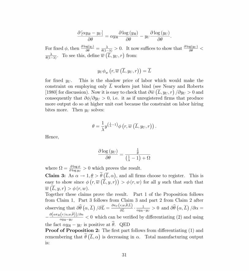
∂ [αyR − yU ]∂θ

= αyR∂ log (yR)

∂θ− yU ∂ log (yU)

∂θ.

For fixed φ, then∂ log(yj)

∂θ= λ

θ(1−λ) > 0. It now suffices to show that∂ log(yU )

∂θ<

λθ(1−λ) . To see this, define w

¡L, yU , r

¢from:

yUφw¡r,w

¡L, yU , r

¢¢= L

for fixed yU . This is the shadow price of labor which would make theconstraint on employing only L workers just bind (see Neary and Roberts[1980] for discussion). Now it is easy to check that ∂w

¡L, yU , r

¢/∂yU > 0 and

consequently that ∂φ/∂yU > 0, i.e. it as if unregistered firms that producemore output do so at higher unit cost because the constraint on labor hiringbites more. Then yU solves:

θ =1

λy(

1λ−1)φ

¡r, w

¡L, yU , r

¢¢.

Hence,

∂ log (yU)

∂θ=

1θ¡

1λ− 1¢+ Ω

where Ω = ∂ logφ∂ log yU

> 0 which proves the result.

Claim 3: As α → 1, θ > eθ ¡L,α¢, and all firms choose to register. This iseasy to show since φ

¡r, w

¡L, y, r

¢¢> φ (r, w) for all y such that such that

w¡L, y, r

¢> φ (r, w).

Together these claims prove the result. Part 1 of the Proposition followsfrom Claim 1, Part 3 follows from Claim 3 and part 2 from Claim 2 after

observing that ∂bθ ¡α, L¢ /∂L = ∂πU(r,w,bθ;L)∂L

· 1αyR−yU > 0 and ∂bθ ¡α, L¢ /∂α =

−∂(απR(r/α,w,bθ))/∂ααyR−yU < 0 which can be verified by differentiating (2) and using

the fact αyR − yU is positive at bθ. QEDProof of Proposition 2: The first part follows from differentiating (1) and

remembering that eθ ¡L,α¢ is decreasing in α. Total manufacturing outputis:

31

y¡r, w,α, L

¢=

Z bθ(α,L)θ

y¡r, w, z;L

¢dz +

Z θ

bθ(α,L) y³ rα, w, z

´dz

Differentiating this with respect to α yields:

hy³r, w,bθ ¡α, L¢ ;L´− y ³ r

α, w,bθ ¡α, L¢´i ∂bθ ¡α, L¢

∂α+

Z θ

bθ(α,L)−rα2

∂y¡rα, w, z

¢∂ (r/α)

dz > 0

sincehy³r, w,bθ ¡α, L¢ ;L´− y ³ r

α, w,bθ ¡α, L¢´i < 0 and ∂bθ(α,L)

∂α< 0. QED

10 Data Appendix

The data used in the paper come from a wide variety of sources.31 Theycover the sixteen main Indian states listed in Table I and span the period1958-1992. Haryana split from the state of Punjab in 1965. From this dateon, we include separate observations for Punjab and Haryana. Variablesexpressed in real terms are deflated using the Consumer Price Index forAgricultural Laborers (CPIAL) andConsumer Price Index for Indus-trial Workers (CPIIW). These are drawn from a number of Government ofIndia publications which include Indian Labor Handbook, the Indian LaborJournal, the Indian Labor Gazette and the Reserve Bank of India Reporton Currency and Finance. Ozler, Datt and Ravallion [1996] have furthercorrected CPIAL and CPIIW to take account of inter-state cost of livingdifferentials and have also adjusted CPIAL to take account of rising firewoodprices. The reference period for the deflator is October 1973- March 1974.Population data used to express magnitudes in per capita terms comesfrom the 1951, 1961, 1971, 1981 and 1991 censuses [Census of India, Regis-trar General and Census Commissioner, Government of India] and has been

31Our data sets builds on Ozler, Datt and Ravallion [1996] which collects published dataon poverty, output, wages, price indices and population to construct a consistent paneldata set on Indian states for the period 1958 to 1992. We are grateful to Martin Ravallionfor providing us with this data and to Guarav Datt for answering various queries. Tothese data, we have added information on labor regulation, manufacturing performance,political representation, infrastructure and public finances of Indian states.

32

interpolated between census years. Separate series are available for urbanand rural areas.The labor regulation variable comes from state specific text amend-

ments to the Industrial Disputes Act 1947 as reported in Malik [1997]. Wedecided to code each change in the following way: a 1 denotes a change thatis pro-worker or anti-employer, a 0 denotes a change that we judged not toaffect the bargaining power of either workers or employers and a −1 denotesa change which we regard to be anti-worker or pro-employer. There were121 state specific amendments which was coded in this manner. Where therewas more than one amendment in a year we collapsed this information intoa single directional measure. Thus reforms in the regulatory climate are re-stricted to taking a value of 1, 0,−1 in any given state and year. To use thesedata, we then construct cumulated variables which map the entire historyof each state beginning from 1947 — the date of enactment of the IndustrialDisputes Act.State output comes from Estimates of State Domestic Product pub-

lished by Department of Statistics, Ministry of Planning, Government ofIndia. Output variables are deflated and expressed in log per capita terms.The breakdown of total output into agricultural, non-agricultural and manu-facturing output is done under the National Industrial Classification System(NIC) which conforms with the International Standard Industrial Classifi-cation System (ISIC). Within manufacturing — registered manufacturing isdefined by the Factories Act of 1948 to refer to firms with ten or more em-ployees with power or twenty or more employees without power. Unregisteredmanufacturing refers to firms below these cutoffs and the size of this sectoris appraised by sample surveys carried out by the Department of Statistics.Figures on employees, workers and mandays come from the Annual

Survey of Industries, Central Statistical Office (Industrial Statistics Wing),Department of Statistics, Ministry of Planning and Programme Implemen-tation, Government of India. Workers are defined as to include all personsemployed directly or through any agency whether for wages or not and en-gaged in any manufacturing process or in any other kind of work incidental toor connected to the manufacturing process. Employees includes all workersand persons receiving wages and holding supervisory or managerial positionsengaged in administrative office, store keeping section and welfare section,sales department as also those engaged in purchase of raw materials etc. orpurchase of fixed assets for the factory and watch and ward staff. Mandaysrepresent the total number of days worked and not the number of days paid

33

for during the accounting year. Daily employment figures are from returnssubmitted from firms under the Factories Act of 1948 which have been an-alyzed and collated in the Indian Labor Yearbook, Labor Bureau, Ministryof Labor, Government of India. They are obtained by dividing total worker(defined as above) attendances in a year by the number of days worked bythe factory.Wages are defined to include all remunerations capable of being ex-

pressed in monetary terms and also payable more or less regularly in eachpay period to workers. It includes (a) direct wages and salary payments, (b)remuneration for period not worked, (c) bonuses and ex-gratia payments paidboth at regular and at less frequent intervals. It excludes (a) lay off paymentswhich are made from trust or other social funds sets up expressly for thispurpose, imputed value of the benefits in kind, (b) employer’s contribution tothe old age benefits and other social security charges, direct expenditure onmaternity benefits and creches and other group benefits, (c) travelling andother expenditure incurred for the business purpose, are re-imbrued by theemployer are excluded. The wages are expressed in terms of gross value i.e.before deduction for fines, damages, taxes, provident funds, employee’s stateinsurance contribution etc. Salaries are defined in the same way as wagesbut paid to all employees plus the imputed value of benefits in kind. Thesecome from the Annual Survey of Industries and are expressed in real termsand per worker or per employee respectively. Annual earnings per workercomes from the Indian Labor Yearbook and is defined as gross workers wagebill divided by daily employment as defined above.Value-added in the registered manufacturing sector is the increment

to the value of goods and services that is contributed by the factory andis obtained by deducting the value of total inputs and depreciations fromthe value of output. The number of factories variable comes from thelist maintained by the Chief Inspector of Factories in each state which isupdated to take into account both deregistration of firms and new entrants.It thus captures the net flow of firms in the registered manufacturing sector.Fixed capital represents the depreciated value of fixed assets owned bythe factory on the closing date of the accounting year. Fixed assets arethose which have a normal productive life of more than one year. Fixedcapital covers all types of assets new or used or own constructed, deployed forproduction, transportation, living or recreational activities, hospitals, schoolsetc for factory personnel. All these measures come from the Annual Surveyof Industries.

34

The data on political histories comes from Butler, Lahiri and Roy[1991]. This primary data is aggregated into four political groupings whichare defined in the text and expressed as shares of the total number of seatsin state legislatures. State political configurations are held constant be-tween elections. Political history is measured by the number if years dur-ing our data period that particular political groupings have held a majorityof the seats in the legislature. In our data period, the relevant groupingsare: the Congress party, the Janata parties, hard left parties and regionalparties. These groupings contain the following parties (i) Congress Party(Indian National Congress + Indian Congress Socialist + Indian NationalCongress Urs + Indian National Congress Organization), (ii) Janata parties(Lok Dal+Janata+Janata Dal), (iii) a hard left grouping (Communist Partyof India + Communist Party of India Marxist), and a (iv) grouping made upof regional parties.The poverty figures we use for the rural and urban areas of India’s

16 major states, spanning 1957-58 to 1991-92 were put together by Ozler,Datt and Ravallion [1996]. These measures are based on 22 rounds of theNational Sample Survey (NSS) which span this period. The NSS roundsare not evenly spaced: the average interval between the midpoints of thesurveys ranges from 0.9 to 5.5 years. Surveys were carried out in the followingyears 1958, 1959, 1960, 1961, 1962, 1963, 1965, 1966, 1967, 1968, 1969,1970, 1971, 1973, 1974, 1978, 1983, 1987, 1988, 1990, 1991, 1992. Becauseother data is typically available on a yearly basis weighted interpolation hasbeen used to generate poverty measures for years where there was no NSSsurvey. The poverty lines used are those recommended by the PlanningCommission [1993]. The headcount and poverty gap measures are estimatedfrom the grouped distributions of per capita expenditure published by theNSS, using parameterized Lorenz curves using a methodology detailed inDatt and Ravallion [1992]

35

Table 1: State Economic Characteristics by Labor Regulation Status

Pro Employer Neutral Pro Worker Registered manufacturing ouput in 1960

35 48 109*

Registered manufacturing output per capita in 1990

149 132 229

Output per capita in 1960 763 822 950

Output per capita in 1990 1380 1463 1574

Population growth (percent)

2.1 2.2 2.2

Total taxes per capita 91 93 97

Development expenditure per capita

93 112 99

Installed electrical capacity per capita

0.03 0.04 0.04

Literacy rate (percent) 40 32 43 Notes: Registered manufacturing and total output figures are expressed in real per capita terms. Population growth is the annual rate of population growth, total taxes refers to all central and state tax revenues allocated to a state; log development expenditure refers to expenditures by state governments on key economic and social services and is expressed in real per capita terms, installed electrical capacity measured in watts is expressed in per capita tems, literacy is the population literacy rate. Figures for population growth, development expenditure, electricity and literacy are averages for the 1960-1990 period. The neutral states are Assam, Bihar, Haryana, Jammu & Kashmir, Punjab and Uttar Pradesh. The pro-employer states Andhra Pradesh, Karnataka, Kerala, Madhya Pradesh, Rajasthan and Tamil Nadu and the pro-worker states are Gujarat, Maharastra, Orissa and West Bengal.

Table 2: Labor Regulation and Output in India: 1958-1992 (1) (2) (3) (4) (5) (6)

Log stateoutput

Log state non-ag output

Log state ag outptut

Log total manu output

Log reg manu output

Log unreg manu output

Lagged dep var 0.544 0.692 0.326 0.609 0.416 0.747

(11.27)** (17.50)** (5.57)** (12.83)** (4.72)** (13.81)**Labor regulation -0.003 -0.010 0.009 -0.026 -0.094 0.020

(0.60) (2.10)* (1.07) (2.84)** (5.05)** (1.99)*Population growth -3.645 -3.528 -0.768 -2.345 3.545 -2.905

(1.97)* (1.89) (0.26) (0.83) (0.85) (0.69)Log electricity 0.012 0.004 0.051 0.008 0.084 -0.037

(0.98) (0.47) (2.52)* (0.52) (3.13)** (1.63)Log dev exp 0.081 0.128 0.055 0.199 0.100 0.196

(2.58)* (4.56)** (1.21) (4.41)** (1.30) (2.81)**Observations 478 473 473 473 473 473R-squared 0.95 0.98 0.88 0.97 0.96 0.93

Notes: Absolute t statistics calculated using robust standard errors are reported in parentheses, * significant at 5%; ** significant at 1%. Total, non-agricultural, agricultural, total manufacturing, registered manufacturing and unregistered manufacturing output figures are all components of state domestic product and are expressed in log real per capita terms. Labor regulation captures the direction of regulatory change in a given state and year (1=pro-worker, 0=neutral, -1=pro-employer) and has been cumulated over the period. Population growth is the annual rate of population growth, log electricity is log installed electrical capacity measured in watts, log development expenditure refers to expenditures by state governments on key economic and social services and is expressed in real log per capita terms. The data are for the sixteen main states for the period 1958 - 1992. Haryana split from the Punjab in 1965. From this date on, we include separate observations for Punjab and Haryana. We therefore have a total of 552 possible observations. Deviations from this are accounted for by missing data. See the Data Appendix for details on the construction and sources of the variables.

Table 3: Labor Regulation and Employment in Registered Manufacturing in India: 1958-1992 (1) (2) (3) (4) Log employees Log workers Log mandays Log daily

employment Lagged dep var 0.603 0.690 0.780 0.614

(4.28)** (9.39)** (21.40)** (6.20)**Labor regulation -0.046 -0.032 -0.031 -0.245

(2.74)** (2.19)* (3.96)** (3.27)**Population growth 13.887 -2.021 7.193 -6.463

(2.45)* (0.48) (3.41)** (0.85)Log electricity -0.002 0.043 0.001 0.048

(0.09) (2.08)* (0.05) (1.35)Log dev exp 0.015 0.090 0.015 0.231

(0.32) (1.54) (0.39) (1.62)Observations 511 512 513 441R-squared 0.99 0.96 0.99 0.94

Notes: Absolute t statistics calculated using robust standard errors are reported in parentheses, * significant at 5%; ** significant at 1%. Employees and workers refer to numbers employed where the former contains those in supervisory or managerial positions in addition to workers. Mandays is defined as the total number of days worked in a year whereas daily employment is defined as total worker attendances over a year divided by the total number of days worked. All employment variables refer to the registered manufacturing sector and are expressed in log terms. Labor regulation captures the direction of regulatory change in a given state and year (1=pro-worker, 0=neutral, -1=pro-employer) and has been cumulated over the period. Population growth is the annual rate of population growth, log electricity is log installed electrical capacity measured in watts, log development expenditure refers to expenditures by state governments on key economic and social services and is expressed in real log per capita terms. The data are for the sixteen main states for the period 1958 - 1992. Haryana split from the Punjab in 1965. From this date on, we include separate observations for Punjab and Haryana. We therefore have a total of 552 possible observations. Deviations from this are accounted for by missing data. See the Data Appendix for details on the construction and sources of the variables.

Table 4: Output, Employment and Poverty Effects of Labor Regulation

(1) (2) (3)State Manufacturing Output Manufacturing Employment Urban Headcount

Andrha Pradesh 84% 94% 110% Karnataka 98% 99% 101%

Kerala 96% 99% 103%Madhya Pradesh 96% 99% 102%

Rajasthan 89% 96% 107%Tamil Nadu 88% 96% 107%

Gujarat 106% 102% 97%Maharashtra 107% 102% 97%

Orissa 103% 101% 98%West Bengal 114% 104% 90%

Notes: The figures represent what manufacturing output, employment and urban poverty would have been in 1990 had states not passed any pro-labor or pro-firm amendments expressed as a ratio of actual figures for 1990. Results obtained by using estimated effect as predicted by the coefficient in Tables 2, 3 and 10. We only present results for pro-labor and pro-firm states as the ratio for neutral states is by definition one. Manufacturing ouptut is defined as log real registered manufacturing output per capita. Manufacturing employment is defined as log mandays in registered manufacturing. Poverty is defined as the proportion of the population beneath the urban poverty line.

Table 5: Labor Regulation and Wages and Earnings in India: 1958- 1992 (1) (2) (3) (4)

Log wages per worker

Log salary per employee

Log salary per manday

Log annual earnings per worker

Lagged dep var 0.642 0.281 0.367 0.356

(5.83)** (3.81)** (2.78)** (5.08)**

Labor regulation -0.009 -0.006 0.008 -0.028

(0.63) (0.35) (0.41) (1.29)

Population growth 10.065 9.037 1.336 -0.525

(2.04)* (1.20) (0.53) (0.13)

Log electricity -0.020 -0.049 0.007 -0.019

(0.95) (0.94) (0.27) (0.87)

Log dev exp -0.006 0.199 0.149 0.176

(0.09) (3.54)** (3.12)** (2.48)*

Observations 509 507 507 443

R-squared 0.85 0.82 0.79 0.69Notes: Absolute t statistics calculated using robust standard errors are reported in parentheses, * significant at 5%; ** significant at 1%. Wages refers to all remunerations payable to workers whereas salaries refers to renumerations payable to employees. Annual earnings per worker is defined as the gross workers wage bill divided by daily employment. All earning figures are expressed in real log terms. Labor regulation captures the direction of regulatory change in a given state and year (1=pro-worker, 0=neutral, -1=pro-employer) and has been cumulated over the period. Population growth is the annual rate of population growth, log electricity is log installed electrical capacity measured in watts, log development expenditure refers to expenditures by state governments on key economic and social services and is expressed in real log per capita terms. The data are for the sixteen main states for the period 1958 - 1992. Haryana split from the Punjab in 1965. From this date on, we include separate observations for Punjab and Haryana. We therefore have a total of 552 possible observations. Deviations from this are accounted for by missing data. See the Data Appendix for details on the construction and sources of the variables.

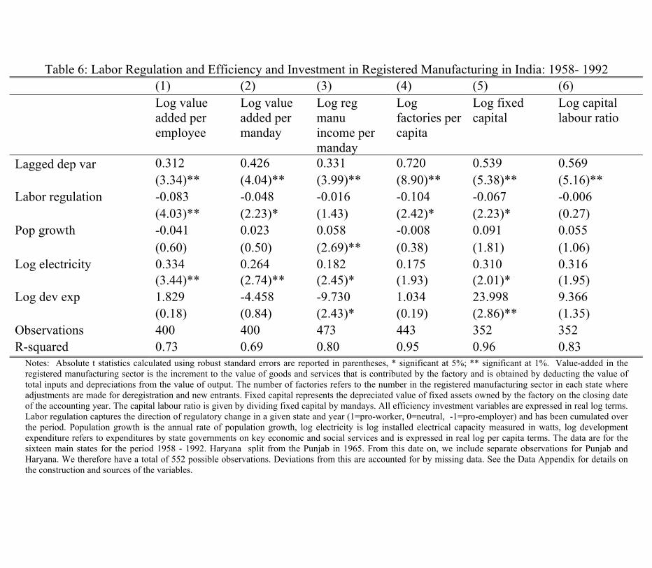
Table 6: Labor Regulation and Efficiency and Investment in Registered Manufacturing in India: 1958- 1992 (1) (2) (3) (4) (5) (6) Log value

added per employee

Log value added per manday

Log reg manu income per manday

Log factories per capita

Log fixed capital

Log capital labour ratio

Lagged dep var 0.312 0.426 0.331 0.720 0.539 0.569 (3.34)** (4.04)** (3.99)** (8.90)**

(5.38)** (5.16)**Labor regulation

-0.083 -0.048 -0.016 -0.104 -0.067 -0.006(4.03)** (2.23)* (1.43) (2.42)* (2.23)* (0.27)

Pop growth -0.041 0.023 0.058 -0.008 0.091 0.055(0.60) (0.50) (2.69)** (0.38) (1.81) (1.06)

Log electricity

0.334 0.264 0.182 0.175 0.310 0.316(3.44)** (2.74)** (2.45)* (1.93) (2.01)* (1.95)

Log dev exp 1.829 -4.458 -9.730 1.034 23.998 9.366(0.18) (0.84) (2.43)* (0.19) (2.86)** (1.35)

Observations 400 400 473 443 352 352R-squared 0.73 0.69 0.80 0.95 0.96 0.83

Notes: Absolute t statistics calculated using robust standard errors are reported in parentheses, * significant at 5%; ** significant at 1%. Value-added in the registered manufacturing sector is the increment to the value of goods and services that is contributed by the factory and is obtained by deducting the value of total inputs and depreciations from the value of output. The number of factories refers to the number in the registered manufacturing sector in each state where adjustments are made for deregistration and new entrants. Fixed capital represents the depreciated value of fixed assets owned by the factory on the closing date of the accounting year. The capital labour ratio is given by dividing fixed capital by mandays. All efficiency investment variables are expressed in real log terms. Labor regulation captures the direction of regulatory change in a given state and year (1=pro-worker, 0=neutral, -1=pro-employer) and has been cumulated over the period. Population growth is the annual rate of population growth, log electricity is log installed electrical capacity measured in watts, log development expenditure refers to expenditures by state governments on key economic and social services and is expressed in real log per capita terms. The data are for the sixteen main states for the period 1958 - 1992. Haryana split from the Punjab in 1965. From this date on, we include separate observations for Punjab and Haryana. We therefore have a total of 552 possible observations. Deviations from this are accounted for by missing data. See the Data Appendix for details on the construction and sources of the variables.

Table 7: Checking Robustness to Introducing Aggregate Number of Regulatory Changes (1) (2) (3) (4) (5) (6) (7) (8) Log reg

manu output per capita

Log reg manu output per capita

Log mandays

Log mandays

Log value added per worker

Log value added per worker

Log fixed capital

Log fixed capital

Lag dep var 0.467 0.414 0.806 0.780 0.332 0.304 0.557 0.537 (5.11)**

(4.70)** (24.12)**

(21.49)**

(3.45)**

(3.22)** (5.85)**

(5.34)**Labor regul

-0.084 -0.034 -0.096 -0.076(4.22)** (3.68)**

(3.83)** (2.24)*

Total changes

-0.011 -0.004 -0.001 0.001 0.000 0.007 0.001 0.006(3.20)**

(1.21) (0.93) (0.89) (0.02) (1.58) (0.32) (1.30)

Pop growth

3.014 3.684 6.808 7.121 4.005 1.792 25.253 24.126(0.70) (0.88) (3.19)**

(3.39)** (0.39) (0.18) (2.85)** (2.87)**

Log electricity

0.108 0.088 0.007 -0.000 -0.017 -0.046 0.106 0.087(3.33)** (3.13)** (0.46) (0.03) (0.26) (0.66) (2.18)* (1.70)

Log dev exp

0.074 0.093 0.013 0.015 0.308 0.329 0.283 0.304(0.87) (1.19) (0.36) (0.40) (3.17)**

(3.45)**

(1.90) (2.00)*

Observations 473 473 513 513 400 400 352 352R-squared 0.96 0.96 0.99 0.99 0.72 0.73 0.96 0.96Notes: Absolute t statistics calculated using robust standard errors are reported in parentheses, * significant at 5%; ** significant at 1%. Output is defined in log real per capita terms. Mandays is defined as the total number of days worked in a year and is expressed in log terms. Value-added is the increment to the value of goods and services and is obtained by deducting the value of total inputs and depreciations from the value of output. Fixed capital represents the depreciated value of fixed assets owned by the factory on the closing date of the accounting year. All these variables are for the registered manufacturing sector. Total changes refers to the total number of state level legislative changes made to the Industrial Disputes Act. Labor regulation captures the direction of regulatory change in a given state and year (1=pro-worker, 0=neutral, -1=pro-employer) and has been cumulated over the period. Population growth is the annual rate of population growth, log electricity is log installed electrical capacity measured in watts, log development expenditure refers to expenditures by state governments on key economic and social services and is expressed in real log per capita terms. The data are for the sixteen main states for the period 1958 - 1992. Haryana split from the Punjab in 1965. From this date on, we include separate observations for Punjab and Haryana. We therefore have a total of 552 possible observations. Deviations from this are accounted for by missing data. See the Data Appendix for details on the construction and sources of the variables.

Table 8: Checking Robustness to Introducing Within Year State Rank (1) (2) (3) (4) (5) Log reg

manu output

Log mandays Log salary per manday

Log value added per employee

Log fixed capital

Lagged dep var 0.475 0.802 0.368 0.312 0.543 (5.13)** (23.40)** (2.79)**

(3.34)** (5.50)**Within year state rank -0.003 -0.001 0.000 -0.005 -0.003

(2.68)** (2.19)* (0.26) (3.75)** (2.14)*Pop growth 3.332 6.985 1.234 2.822 24.763

(0.76) (3.29)** (0.50) (0.28) (2.89)**Log electricity

0.103 0.006 0.005 -0.031 0.099(3.33)** (0.39) (0.17) (0.45) (2.03)*

Log dev exp 0.094 0.014 0.149 0.325 0.300 (1.14) (0.38) (3.11)** (3.36)** (1.97)

Observations 473 513 507 400 352R-squared 0.96 0.99 0.79 0.73 0.96Notes: Absolute t statistics calculated using robust standard errors are reported in parentheses, * significant at 5%; ** significant at 1%. Output is defined in log real per capita terms. Mandays is defined as the total number of days worked in a year and is expressed in log terms. Value-added is the increment to the value of goods and services and is obtained by deducting the value of total inputs and depreciations from the value of output. Fixed capital represents the depreciated value of fixed assets owned by the factory on the closing date of the accounting year. All these variables are for the registered manufacturing sector. Labor regulation captures the direction of regulatory change in a given state and year (1=pro-worker, 0=neutral, -1=pro-employer) and has been cumulated over the period. Population growth is the annual rate of population growth, log electricity is log installed electrical capacity measured in watts, log development expenditure refers to expenditures by state governments on key economic and social services and is expressed in real log per capita terms. The data are for the sixteen main states for the period 1958 - 1992. Haryana split from the Punjab in 1965. From this date on, we include separate observations for Punjab and Haryana. We therefore have a total of 552 possible observations. Deviations from this are accounted for by missing data. See the Data Appendix for details on the construction and sources of the variables.

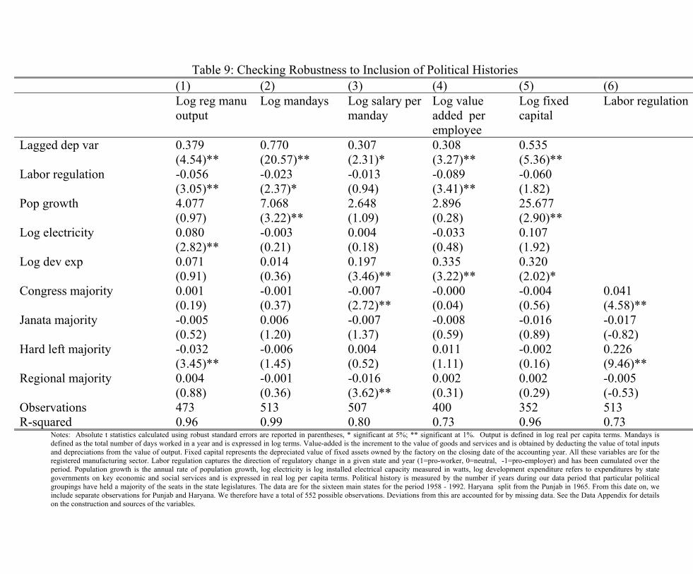
Table 9: Checking Robustness to Inclusion of Political Histories (1) (2) (3) (4) (5) (6)

Log reg manu output

Log mandays Log salary per manday

Log value added per employee

Log fixed capital

Labor regulation

Lagged dep var 0.379 0.770 0.307 0.308 0.535 (4.54)** (20.57)** (2.31)* (3.27)** (5.36)**

Labor regulation

-0.056 -0.023 -0.013 -0.089 -0.060(3.05)** (2.37)* (0.94) (3.41)** (1.82)

Pop growth 4.077 7.068 2.648 2.896 25.677(0.97) (3.22)** (1.09) (0.28) (2.90)**

Log electricity

0.080 -0.003 0.004 -0.033 0.107(2.82)** (0.21) (0.18) (0.48) (1.92)

Log dev exp 0.071 0.014 0.197 0.335 0.320(0.91) (0.36) (3.46)** (3.22)** (2.02)*

Congress majority 0.001 -0.001 -0.007 -0.000 -0.004 0.041 (0.19) (0.37) (2.72)** (0.04) (0.56) (4.58)** Janata majority

-0.005 0.006 -0.007 -0.008 -0.016 -0.017(0.52) (1.20) (1.37) (0.59) (0.89) (-0.82)

Hard left majority

-0.032 -0.006 0.004 0.011 -0.002 0.226 (3.45)** (1.45) (0.52) (1.11) (0.16) (9.46)**

Regional majority

0.004 -0.001 -0.016 0.002 0.002 -0.005 (0.88) (0.36) (3.62)** (0.31) (0.29) (-0.53)

Observations 473 513 507 400 352 513R-squared 0.96 0.99 0.80 0.73 0.96 0.73

Notes: Absolute t statistics calculated using robust standard errors are reported in parentheses, * significant at 5%; ** significant at 1%. Output is defined in log real per capita terms. Mandays is defined as the total number of days worked in a year and is expressed in log terms. Value-added is the increment to the value of goods and services and is obtained by deducting the value of total inputs and depreciations from the value of output. Fixed capital represents the depreciated value of fixed assets owned by the factory on the closing date of the accounting year. All these variables are for the registered manufacturing sector. Labor regulation captures the direction of regulatory change in a given state and year (1=pro-worker, 0=neutral, -1=pro-employer) and has been cumulated over the period. Population growth is the annual rate of population growth, log electricity is log installed electrical capacity measured in watts, log development expenditure refers to expenditures by state governments on key economic and social services and is expressed in real log per capita terms. Political history is measured by the number if years during our data period that particular political groupings have held a majority of the seats in the state legislatures. The data are for the sixteen main states for the period 1958 - 1992. Haryana split from the Punjab in 1965. From this date on, we include separate observations for Punjab and Haryana. We therefore have a total of 552 possible observations. Deviations from this are accounted for by missing data. See the Data Appendix for details on the construction and sources of the variables.

Table 10: Labor Regulation and Poverty in India: 1958-1992 (1) (2) (3) (4) (5)

Urbanheadcount

Urban poverty gap

Rural poverty gap

Rural-urban poverty gap difference

Rural-urban headcount difference

GLS GLS GLS GLS GLS

Labor regulation 1.815 0.550 0.020 -0.548 -2.266

(4.97)** (2.85)** (0.07) (1.83) (3.60)**

Population growth -197.176 -179.161 -269.790 -89.197 -54.597

(1.73) (3.10)** (3.40)** (1.21) (0.32)

Log electricity 0.756 0.360 0.051 -0.325 -0.773

(1.39) (1.66) (0.19) (1.13) (1.03)

Log dev exp 3.259 0.594 1.012 0.511 -1.608

(2.26)* (0.97) (1.25) (0.58) (0.75)

Observations 513 513 513 513 513Notes: Absolute t statistics calculated using robust standard errors are reported in parentheses, * significant at 5%; ** significant at 1%. Poverty measures in other regressions have been interpolated between survey years. In columns (4) the poverty gap difference is the difference between the rural and urban poverty gap measures for each state. In column (5), the headcount difference is the difference between the rural and urban headcount index for each state. See the Data Appendix for details on the construction and sources of the variables. The data are for the sixteen main states for the period 1958 - 1992. Haryana split from the Punjab in 1965. From this date on, we include separate observations for Punjab and Haryana. We therefore have a total of 552 possible observations. Deviations from this are accounted for by missing data. Labor regulation captures the direction of regulatory change in a given state and year (1=pro-worker, 0=neutral, -1=pro-employer) and has been cumulated over the period. Population growth is the annual rate of population growth, log electricity is log installed electrical capacity measured in watts, log development expenditure refers to expenditures by state governments on key economic and social services and is expressed in real log per capita terms.

dire

ctio

n of

labo

r reg

ulat

ion

Figure 1: Labour Regulation in India: 1958-1992year

Andra Pradesh

-4

-2

0

2

4Assam Bihar Gujarat

Haryana

-4

-2

0

2

4Jammu & Kashmir Karnataka Kerala

Madhya Pradesh

-4

-2

0

2

4Maharashtra Orissa Punjab

Rajasthan

1960 1970 1980 1990-4

-2

0

2

4Tamil Nadu

1960 1970 1980 1990

Uttar Pradesh

1960 1970 1980 1990

West Bengal

1960 1970 1980 1990

regi

ster

ed m

anuf

actu

ring

outp

ut

Figure 2: Registered Manufacturing Output Per Capita: 1958-1992year

Andra Pradesh

0

100

200

300

400Assam Bihar Gujarat

Haryana

0

100

200

300

400Jammu & Kashmir Karnataka Kerala

Madhya Pradesh

0

100

200

300

400Maharashtra Orissa Punjab

Rajasthan

1960 1970 1980 19900

100

200

300

400Tamil Nadu

1960 1970 1980 1990

Uttar Pradesh

1960 1970 1980 1990

West Bengal

1960 1970 1980 1990

regi

ster

ed m

anuf

actu

ring

empl

oym

Figure 3: Registered Manufacturing Employment: 1958-1992year

Andra Pradesh

0

400

800

1200

1600Assam Bihar Gujarat

Haryana

0

400

800

1200

1600Jammu & Kashmir Karnataka Kerala

Madhya Pradesh

0

400

800

1200

1600Maharashtra Orissa Punjab

Rajasthan

1960 1970 1980 19900

400

800

1200

1600Tamil Nadu

1960 1970 1980 1990

Uttar Pradesh

1960 1970 1980 1990

West Bengal

1960 1970 1980 1990