CAMERA CALIBRATION - Computer Science calibration is a necessary step in 3D computer vision in order...

Chapter 2

CAMERA CALIBRATION

Zhengyou Zhang

Camera calibration is a necessary step in 3D computer vision in order toextract metric information from 2D images. It has been studied extensivelyin computer vision and photogrammetry, and even recently new techniqueshave been proposed. In this chapter, we review the techniques proposedin the literature include those using 3D apparatus (two or three planes or-thogonal to each other, or a plane undergoing a pure translation, etc.), 2Dobjects (planar patterns undergoing unknown motions), 1D objects (wandwith dots) and unknown scene points in the environment (self-calibration).The focus is on presenting these techniques within a consistent framework.

2.1 Introduction

Camera calibration is a necessary step in 3D computer vision in order toextract metric information from 2D images. Much work has been done,starting in the photogrammetry community (see [3, 6] to cite a few), andmore recently in computer vision ([12, 11, 33, 10, 37, 35, 22, 9] to cite a few).According to the dimension of the calibration objects, we can classify thosetechniques roughly into three categories.

3D reference object based calibration. Camera calibration is performedby observing a calibration object whose geometry in 3-D space is knownwith very good precision. Calibration can be done very efficiently [8].The calibration object usually consists of two or three planes orthog-onal to each other. Sometimes, a plane undergoing a precisely knowntranslation is also used [33], which equivalently provides 3D referencepoints. This approach requires an expensive calibration apparatus and

5

6 Camera Calibration Chapter 2

an elaborate setup.

2D plane based calibration. Techniques in this category requires to ob-serve a planar pattern shown at a few different orientations [42, 31].Different from Tsai’s technique [33], the knowledge of the plane motionis not necessary. Because almost anyone can make such a calibrationpattern by him/her-self, the setup is easier for camera calibration.

1D line based calibration. Calibration objects used in this category arecomposed of a set of collinear points [44]. As will be shown, a cameracan be calibrated by observing a moving line around a fixed point, suchas a string of balls hanging from the ceiling.

Self-calibration. Techniques in this category do not use any calibrationobject, and can be considered as 0D approach because only imagepoint correspondences are required. Just by moving a camera in astatic scene, the rigidity of the scene provides in general two con-straints [22, 21] on the cameras’ internal parameters from one cameradisplacement by using image information alone. Therefore, if imagesare taken by the same camera with fixed internal parameters, cor-respondences between three images are sufficient to recover both theinternal and external parameters which allow us to reconstruct 3-Dstructure up to a similarity [20, 17]. Although no calibration objectsare necessary, a large number of parameters need to be estimated, re-sulting in a much harder mathematical problem.

Other techniques exist: vanishing points for orthogonal directions [4, 19],and calibration from pure rotation [16, 30].

Before going further, I’d like to point out that no single calibration tech-nique is the best for all. It really depends on the situation a user needs todeal with. Following are my few recommendations:

– Calibration with apparatus vs. self-calibration. Whenever possible, ifwe can pre-calibrate a camera, we should do it with a calibration appa-ratus. Self-calibration cannot usually achieve an accuracy comparablewith that of pre-calibration because self-calibration needs to estimate alarge number of parameters, resulting in a much harder mathematicalproblem. When pre-calibration is impossible (e.g., scene reconstructionfrom an old movie), self-calibration is the only choice.

– Partial vs. full self-calibration. Partial self-calibration refers to thecase where only a subset of camera intrinsic parameters are to be cal-

Section 2.2. Notation and Problem Statement 7

ibrated. Along the same line as the previous recommendation, when-ever possible, partial self-calibration is preferred because the numberof parameters to be estimated is smaller. Take an example of 3D re-construction with a camera with variable focal length. It is preferableto pre-calibrate the pixel aspect ratio and the pixel skewness.

– Calibration with 3D vs. 2D apparatus. Highest accuracy can usually beobtained by using a 3D apparatus, so it should be used when accuracy isindispensable and when it is affordable to make and use a 3D apparatus.From the feedback I received from computer vision researchers andpractitioners around the world in the last couple of years, calibrationwith a 2D apparatus seems to be the best choice in most situationsbecause of its ease of use and good accuracy.

– Calibration with 1D apparatus. This technique is relatively new, and itis hard for the moment to predict how popular it will be. It, however,should be useful especially for calibration of a camera network. Tocalibrate the relative geometry between multiple cameras as well astheir intrinsic parameters, it is necessary for all involving cameras tosimultaneously observe a number of points. It is hardly possible toachieve this with 3D or 2D calibration apparatus1 if one camera ismounted in the front of a room while another in the back. This is nota problem for 1D objects. We can for example use a string of ballshanging from the ceiling.

This chapter is organized as follows. Section 2.2 describes the cameramodel and introduces the concept of the absolute conic which is importantfor camera calibration. Section 2.3 presents the calibration techniques usinga 3D apparatus. Section 2.4 describes a calibration technique by observing afreely moving planar pattern (2D object). Its extension for stereo calibrationis also addressed. Section 2.5 describes a relatively new technique which usesa set of collinear points (1D object). Section 2.6 briefly introduces the self-calibration approach and provides references for further reading. Section 2.7concludes the chapter with a discussion on recent work in this area.

2.2 Notation and Problem Statement

We start with the notation used in this chapter.

1An exception is when those apparatus are made transparent; then the cost would bemuch higher.


2.2.1 Pinhole Camera Model

CC

θθ

αβ

),( 00 vu

=ZYX

M

mm

),( tRFigure 2.1. Pinhole camera model

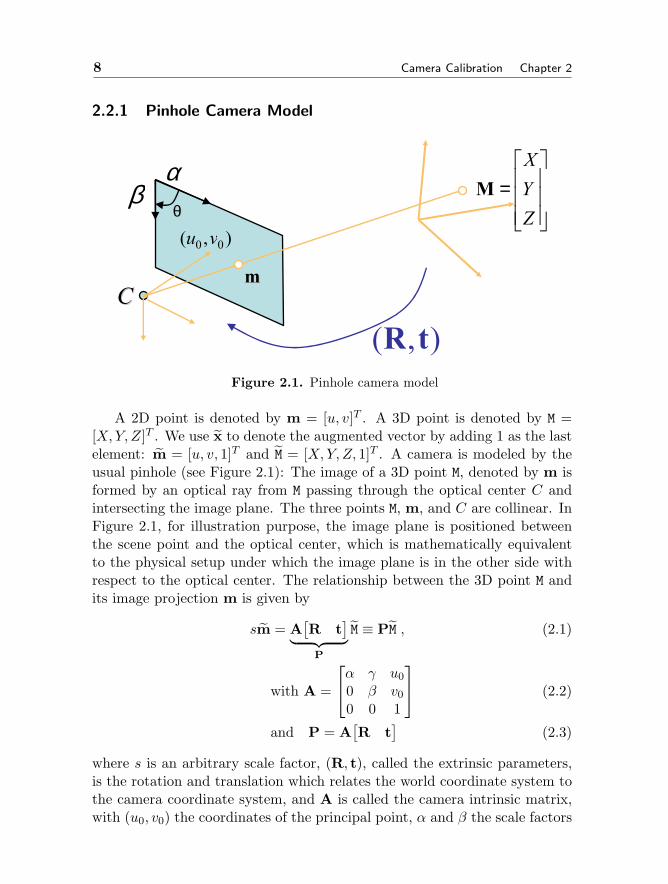
A 2D point is denoted by m = [u, v]T . A 3D point is denoted by M =[X,Y, Z]T . We use x to denote the augmented vector by adding 1 as the lastelement: m = [u, v, 1]T and M = [X,Y, Z, 1]T . A camera is modeled by theusual pinhole (see Figure 2.1): The image of a 3D point M, denoted by m isformed by an optical ray from M passing through the optical center C andintersecting the image plane. The three points M, m, and C are collinear. InFigure 2.1, for illustration purpose, the image plane is positioned betweenthe scene point and the optical center, which is mathematically equivalentto the physical setup under which the image plane is in the other side withrespect to the optical center. The relationship between the 3D point M andits image projection m is given by

sm = A[R t

]︸︷︷︸P

M ≡ PM , (2.1)

with A =

α γ u00 β v00 0 1

(2.2)

and P = A[R t

](2.3)

where s is an arbitrary scale factor, (R, t), called the extrinsic parameters,is the rotation and translation which relates the world coordinate system tothe camera coordinate system, and A is called the camera intrinsic matrix,with (u0, v0) the coordinates of the principal point, α and β the scale factors

Section 2.2. Notation and Problem Statement 9

in image u and v axes, and γ the parameter describing the skew of thetwo image axes. The 3× 4 matrix P is called the camera projection matrix,which mixes both intrinsic and extrinsic parameters. In Figure 2.1, the anglebetween the two image axes is denoted by θ, and we have γ = α cot θ. If thepixels are rectangular, then θ = 90 and γ = 0.

The task of camera calibration is to determine the parameters of thetransformation between an object in 3D space and the 2D image observed bythe camera from visual information (images). The transformation includes

– Extrinsic parameters (sometimes called external parameters): orienta-tion (rotation) and location (translation) of the camera, i.e., (R, t);

– Intrinsic parameters (sometimes called internal parameters): charac-teristics of the camera, i.e., (α, β, γ, u0, v0).

The rotation matrix, although consisting of 9 elements, only has 3 degreesof freedom. The translation vector t obviously has 3 parameters. Therefore,there are 6 extrinsic parameters and 5 intrinsic parameters, leading to intotal 11 parameters.

We use the abbreviation A−T for (A−1)T or (AT )−1.

2.2.2 Absolute Conic

Now let us introduce the concept of the absolute conic. For more details,the reader is referred to [7, 15].

A point x in 3D space has projective coordinates x = [x1, x2, x3, x4]T .The equation of the plane at infinity, Π∞, is x4 = 0. The absolute conic Ωis defined by a set of points satisfying the equation

x21 + x2

2 + x23 = 0x4 = 0 .

(2.4)

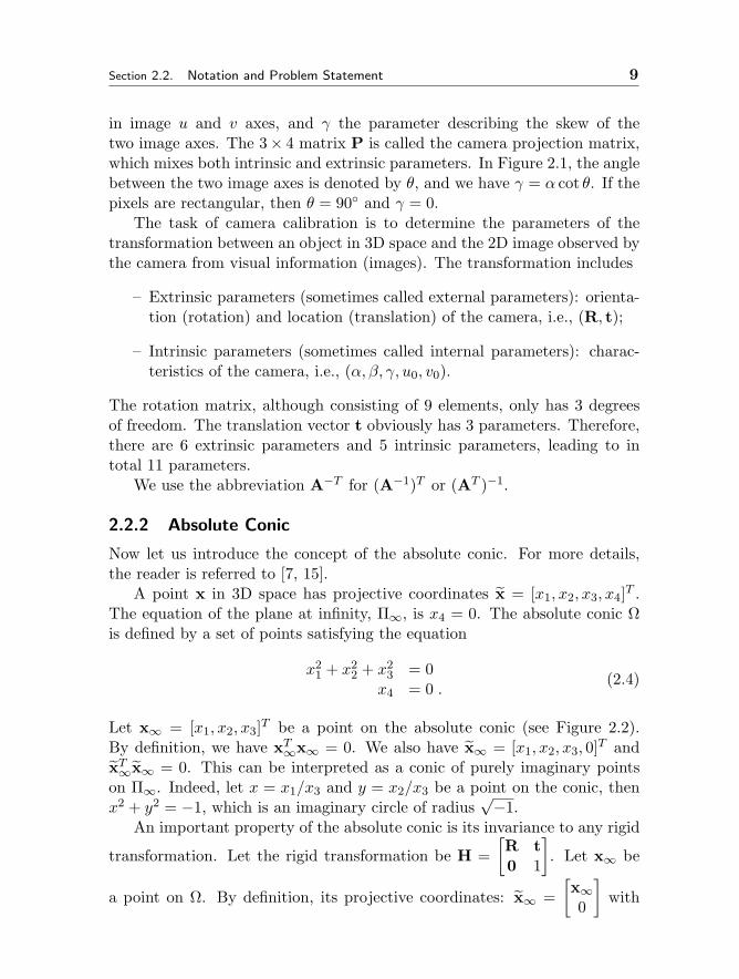
Let x∞ = [x1, x2, x3]T be a point on the absolute conic (see Figure 2.2).By definition, we have xT∞x∞ = 0. We also have x∞ = [x1, x2, x3, 0]T andxT∞x∞ = 0. This can be interpreted as a conic of purely imaginary pointson Π∞. Indeed, let x = x1/x3 and y = x2/x3 be a point on the conic, thenx2 + y2 = −1, which is an imaginary circle of radius

√−1.An important property of the absolute conic is its invariance to any rigid

transformation. Let the rigid transformation be H =[R t0 1

]. Let x∞ be

a point on Ω. By definition, its projective coordinates: x∞ =[x∞0

]with


Plane at infinity

01 =∞−−

∞ mAAm TT

C

∞m

∞x

Absolute Conic

0=∞∞xxT

Image of Absolute Conic

Figure 2.2. Absolute conic and its image

xT∞x∞ = 0. The point after the rigid transformation is denoted by x′∞, and

x′∞ = Hx∞ =

[Rx∞

0

].

Thus, x′∞ is also on the plane at infinity. Furthermore, x′∞ is on the sameΩ because

x′T∞x′

∞ = (Rx∞)T (Rx∞) = xT∞(RTR)x∞ = 0 .

The image of the absolute conic, denoted by ω, is also an imaginary conic,and is determined only by the intrinsic parameters of the camera. This canbe seen as follows. Consider the projection of a point x∞ on Ω, denoted by

Section 2.3. Camera Calibration with 3D Objects 11

m∞, which is given by

m∞ = sA[R t][x∞0

]= sARx∞ .

It follows that

mTA−TA−1m = s2xT∞RTRx∞ = s2xT∞x∞ = 0 .

Therefore, the image of the absolute conic is an imaginary conic, and isdefined by A−TA−1. It does not depend on the extrinsic parameters of thecamera.

If we can determine the image of the absolute conic, then we can solvethe camera’s intrinsic parameters, and the calibration is solved.

We will show several ways in this chapter how to determine ω, the imageof the absolute conic.

2.3 Camera Calibration with 3D Objects

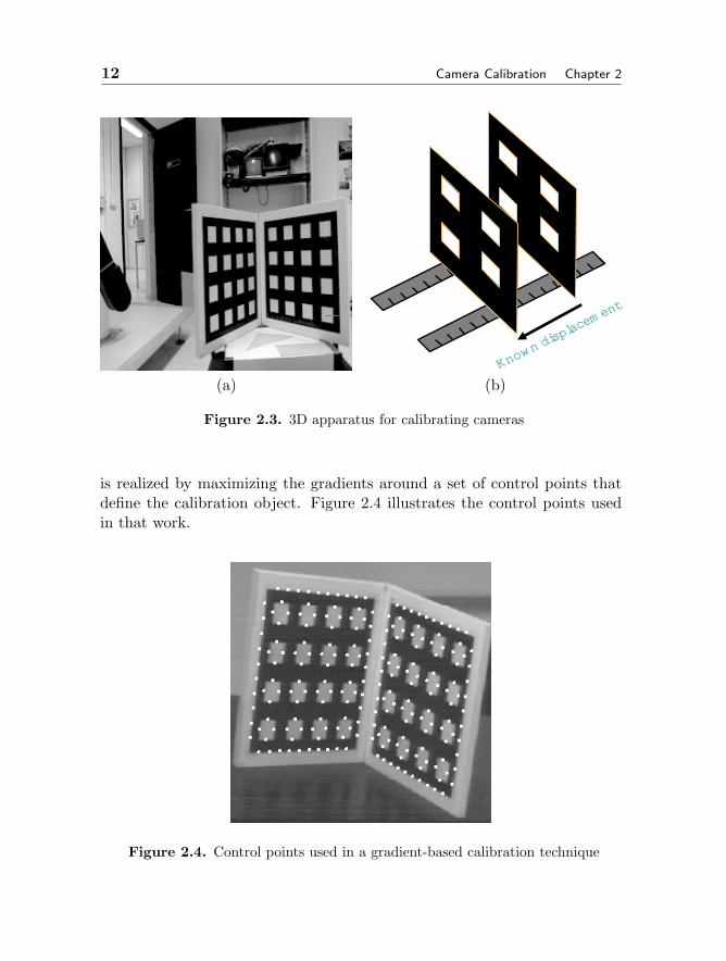
The traditional way to calibrate a camera is to use a 3D reference objectsuch as those shown in Figure 2.3. In Fig. 2.3a, the calibration apparatusused at INRIA [8] is shown, which consists of two orthogonal planes, oneach a checker pattern is printed. A 3D coordinate system is attached tothis apparatus, and the coordinates of the checker corners are known veryaccurately in this coordinate system. A similar calibration apparatus is acube with a checker patterns painted in each face, so in general three faceswill be visible to the camera. Figure 2.3b illustrates the device used in Tsai’stechnique [33], which only uses one plane with checker pattern, but the planeneeds to be displaced at least once with known motion. This is equivalentto knowing the 3D coordinates of the checker corners.

A popular technique in this category consists of four steps [8]:

1. Detect the corners of the checker pattern in each image;

2. Estimate the camera projection matrix P using linear least squares;

3. Recover intrinsic and extrinsic parameters A, R and t from P;

4. Refine A, R and t through a nonlinear optimization.

Note that it is also possible to first refine P through a nonlinear optimization,and then determine A, R and t from the refined P.

It is worth noting that using corners is not the only possibility. We canavoid corner detection by working directly in the image. In [25], calibration


Know

n disp

lacem

ent

Know

n disp

lacem

ent

(a) (b)

Figure 2.3. 3D apparatus for calibrating cameras

is realized by maximizing the gradients around a set of control points thatdefine the calibration object. Figure 2.4 illustrates the control points usedin that work.

Figure 2.4. Control points used in a gradient-based calibration technique


2.3.1 Feature Extraction

If one uses a generic corner detector, such as Harris corner detector, to detectthe corners in the check pattern image, the result is usually not good becausethe detector corners have poor accuracy (about one pixel). A better solutionis to leverage the known pattern structure by first estimating a line for eachside of the square and then computing the corners by intersecting the fittedlines. There are two common techniques to estimate the lines. The first is tofirst detect edges, and then fit a line to the edges on each side of the square.The second technique is to directly fit a line to each side of a square in theimage such that the gradient on the line is maximized. One possibility is torepresent the line by an elongated Gaussian, and estimate the parametersof the elongated Gaussian by maximizing the total gradient covered by theGaussian. We should note that if the lens distortion is not severe, a bettersolution is to fit just one single line to all the collinear sides. This will leadsa much more accurate estimation of the position of the checker corners.

2.3.2 Linear Estimation of the Camera Projection Matrix

Once we extract the corner points in the image, we can easily establish theircorrespondences with the points in the 3D space because of knowledge ofthe patterns. Based on the projection equation (2.1), we are now able toestimate the camera parameters. However, the problem is quite nonlinear ifwe try to estimate directly A, R and t. If, on the other hand, we estimatethe camera projection matrix P, a linear solution is possible, as to be shownnow.

Given each 2D-3D correspondence mi = (ui, vi) ↔ Mi = (Xi, Yi, Zi), wecan write down 2 equations based on (2.1):[

Xi Yi Zi 1 0 0 0 0 uiXi uiYi uiZi ui0 0 0 0 Xi Yi Zi 1 viXi viYi viZi vi

]︸︷︷︸

Gi

p = 0

where p = [p11, p12, . . . , p34]T and 0 = [0, 0]T .For n point matches, we can stack all equations together:

Gp = 0 with G = [GT1 , . . . ,G

Tn ]T

Matrix G is a 2n× 12 matrix. The projection matrix can now be solved by

minp‖Gp‖2 subject to ‖p‖ = 1


The solution is the eigenvector of GTG associated with the smallest eigen-value.

In the above, in order to avoid the trivial solution p = 0 and consideringthe fact that p is defined up to a scale factor, we have set ‖p‖ = 1. Othernormalizations are possible. In [1], p34 = 1, which, however, introduce a sin-gularity when the correct value of p34 is close to zero. In [10], the constraintp231 + p2

32 + p233 = 1 was used, which is singularity free.

Anyway, the above linear technique minimizes an algebraic distance, andyields a biased estimation when data are noisy. We will present later anunbiased solution.

2.3.3 Recover Intrinsic and Extrinsic Parameters from P

Once the camera projection matrix P is known, we can uniquely recover theintrinsic and extrinsic parameters of the camera. Let us denote the first 3×3submatrix of P by B and the last column of P by b, i.e., P ≡ [B b]. SinceP = A[R t], we have

B = AR (2.5)b = At (2.6)

From (2.5), we have

K ≡ BBT = AAT =

α2 + γ2 + u2

0︸︷︷︸ku

u0 v0 + c β︸︷︷︸kc

u0

u0 v0 + c α︸︷︷︸kc

α2v + v2

0︸︷︷︸kv

v0

u0 v0 1

Because P is defined up to a scale factor, the last element of K = BBT is usu-ally not equal to 1, so we have to normalize it such that K33(the last element) =1. After that, we immediately obtain

u0 = K13 (2.7)v0 = K23 (2.8)

β =√kv − v2

0 (2.9)

γ =kc − u0 v0

β(2.10)

α =√ku − u2

0 − γ2 (2.11)


The solution is unambiguous because: α > 0 and β > 0.Once the intrinsic parameters, or equivalently matrix A, are known, the

extrinsic parameters can be determined from (2.5) and (2.6) as:

R = A−1B (2.12)

t = A−1b . (2.13)

2.3.4 Refine Calibration Parameters Through a Nonlinear Opti-mization

The above solution is obtained through minimizing an algebraic distancewhich is not physically meaningful. We can refine it through maximumlikelihood inference.

We are given n 2D-3D correspondences mi = (ui, vi)↔ Mi = (Xi, Yi, Zi).Assume that the image points are corrupted by independent and identicallydistributed noise. The maximum likelihood estimate can be obtained byminimizing the distances between the image points and their predicted po-sitions, i.e.,

minP

∑i

‖mi − φ(P, Mi)‖2 (2.14)

where φ(P, Mi) is the projection of Mi onto the image according to (2.1).This is a nonlinear minimization problem, which can be solved with the

Levenberg-Marquardt Algorithm as implemented in Minpack [23]. It requiresan initial guess of P which can be obtained using the linear technique de-scribed earlier. Note that since P is defined up to a scale factor, we can setthe element having the largest initial value as 1 during the minimization.

Alternatively, instead of estimating P as in (2.14), we can directly esti-mate the intrinsic and extrinsic parameters, A, R, and t, using the samecriterion. The rotation matrix can be parameterized with three variablessuch as Euler angles or scaled rotation vector.

2.3.5 Lens Distortion

Up to this point, we use the pinhole model to describe a camera. It saysthat the point in 3D space, its corresponding point in image and the camera’soptical center are collinear. This linear projective equation is sometimes notsufficient, especially for low-end cameras (such as WebCams) or wide-anglecameras; lens distortion has to be considered.

According to [33], there are four steps in camera projection including lensdistortion:


Step 1: Rigid transformation from world coordinate system (Xw, Yw, Zw)to camera one (X,Y, Z):

[X Y Z]T = R [Xw Yw Zw]T + t

Step 2: Perspective projection from 3D camera coordinates (X,Y, Z) toideal image coordinates (x, y) under pinhole camera model:

x = fX

Z, y = f

Y

Z

where f is the effective focal length.

Step 3: Lens distortion2:

x = x+ δx , y = y + δy

where (x, y) are the distorted or true image coordinates, and (δx, δy)are distortions applied to (x, y).

Step 4: Affine transformation from real image coordinates (x, y) to framebuffer (pixel) image coordinates (u, v):

u = d−1x x+ u0 , v = d−1

y y + v0 ,

where (u0, v0) are coordinates of the principal point; dx and dy are dis-tances between adjacent pixels in the horizontal and vertical directions,respectively.

There are two types of distortions:

Radial distortion: It is symmetric; ideal image points are distorted alongradial directions from the distortion center. This is caused by imperfectlens shape.

Decentering distortion: This is usually caused by improper lens assem-bly; ideal image points are distorted in both radial and tangential di-rections.

The reader is referred to [29, 3, 6, 37] for more details.2Note that the lens distortion described here is different from Tsai’s treatment. Here,

we go from ideal to real image coordinates, similar to [36].


The distortion can be expressed as power series in radial distance r =√x2 + y2:

δx = x(k1r2 + k2r

4 + k3r6 + · · · ) + [p1(r2 + 2x2) + 2p2xy](1 + p3r

2 + · · · ) ,δy = y(k1r

2 + k2r4 + k3r

6 + · · · ) + [2p1xy + p2(r2 + 2y2)](1 + p3r2 + · · · ) ,

where ki’s are coefficients of radial distortion and pj ’s and coefficients ofdecentering distortion.

Based on the reports in the literature [3, 33, 36], it is likely that thedistortion function is totally dominated by the radial components, and es-pecially dominated by the first term. It has also been found that any moreelaborated modeling not only would not help (negligible when compared withsensor quantization), but also would cause numerical instability [33, 36].

Denote the ideal pixel image coordinates by u = x/dx, and v = y/dy. Bycombining Step 3 and Step 4 and if only using the first two radial distortionterms, we obtain the following relationship between (u, v) and (u, v):

u = u+ (u− u0)[k1(x2 + y2) + k2(x2 + y2)2] (2.15)

v = v + (v − v0)[k1(x2 + y2) + k2(x2 + y2)2] . (2.16)

Following the same reasoning as in (2.14), camera calibration includinglens distortion can be performed by minimizing the distances between theimage points and their predicted positions, i.e.,

minA,R,t,k1,k2

∑i

‖mi − m(A,R, t, k1, k2, Mi)‖2 (2.17)

where m(A,R, t, k1, k2, Mi) is the projection of Mi onto the image accordingto (2.1), followed by distortion according to (2.15) and (2.16).

2.3.6 An Example

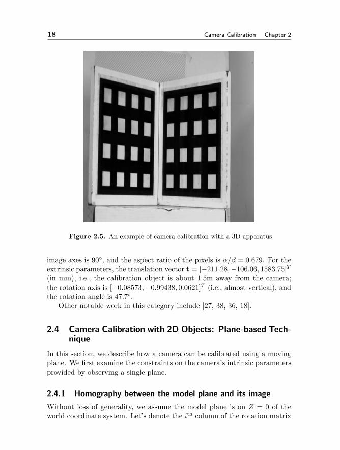
Figure 2.5 displays an image of a 3D reference object, taken by a camera tobe calibrated at INRIA. Each square has 4 corners, and there are in total128 points used for calibration.

Without considering lens distortion, the estimated camera projection ma-trix is

P =

7.025659e−01 −2.861189e−02 −5.377696e−01 6.241890e+012.077632e−01 1.265804e+00 1.591456e−01 1.075646e+014.634764e−04 −5.282382e−05 4.255347e−04 1

From P, we can calculate the intrinsic parameters: α = 1380.12, β =2032.57, γ ≈ 0, u0 = 246.52, and v0 = 243.68. So, the angle between the two


Figure 2.5. An example of camera calibration with a 3D apparatus

image axes is 90, and the aspect ratio of the pixels is α/β = 0.679. For theextrinsic parameters, the translation vector t = [−211.28,−106.06, 1583.75]T

(in mm), i.e., the calibration object is about 1.5m away from the camera;the rotation axis is [−0.08573,−0.99438, 0.0621]T (i.e., almost vertical), andthe rotation angle is 47.7.

Other notable work in this category include [27, 38, 36, 18].

2.4 Camera Calibration with 2D Objects: Plane-based Tech-nique

In this section, we describe how a camera can be calibrated using a movingplane. We first examine the constraints on the camera’s intrinsic parametersprovided by observing a single plane.

2.4.1 Homography between the model plane and its image

Without loss of generality, we assume the model plane is on Z = 0 of theworld coordinate system. Let’s denote the ith column of the rotation matrix

Section 2.4. Camera Calibration with 2D Objects: Plane Based Technique 19

R by ri. From (2.1), we have

s

uv1

= A[r1 r2 r3 t

] XY01

= A[r1 r2 t

] XY1

.

By abuse of notation, we still use M to denote a point on the model plane, butM = [X,Y ]T since Z is always equal to 0. In turn, M = [X,Y, 1]T . Therefore,a model point M and its image m is related by a homography H:

sm = HM with H = A[r1 r2 t

]. (2.18)

As is clear, the 3× 3 matrix H is defined up to a scale factor.

2.4.2 Constraints on the intrinsic parameters

Given an image of the model plane, an homography can be estimated (seeAppendix). Let’s denote it by H = [h1 h2 h3]. From (2.18), we have

[h1 h2 h3] = λA [ r1 r2 t ] ,

where λ is an arbitrary scalar. Using the knowledge that r1 and r2 areorthonormal, we have

hT1 A−TA−1h2 = 0 (2.19)

hT1 A−TA−1h1 = hT2 A−TA−1h2 . (2.20)

These are the two basic constraints on the intrinsic parameters, given onehomography. Because a homography has 8 degrees of freedom and thereare 6 extrinsic parameters (3 for rotation and 3 for translation), we can onlyobtain 2 constraints on the intrinsic parameters. Note that A−TA−1 actuallydescribes the image of the absolute conic [20]. In the next subsection, wewill give an geometric interpretation.

2.4.3 Geometric Interpretation

We are now relating (2.19) and (2.20) to the absolute conic [22, 20].It is not difficult to verify that the model plane, under our convention, is

described in the camera coordinate system by the following equation:

[r3rT3 t

]T xyzw

= 0 ,


where w = 0 for points at infinity and w = 1 otherwise. This plane intersects

the plane at infinity at a line, and we can easily see that[r10

]and

[r20

]are

two particular points on that line. Any point on it is a linear combinationof these two points, i.e.,

x∞ = a

[r10

]+ b

[r20

]=[ar1 + br2

0

].

Now, let’s compute the intersection of the above line with the absoluteconic. By definition, the point x∞, known as the circular point [26], satisfies:xT∞x∞ = 0, i.e., (ar1 + br2)T (ar1 + br2) = 0, or a2 + b2 = 0 . The solutionis b = ±ai, where i2 = −1. That is, the two intersection points are

x∞ = a

[r1 ± ir2

0

].

The significance of this pair of complex conjugate points lies in the fact thatthey are invariant to Euclidean transformations. Their projection in theimage plane is given, up to a scale factor, by

m∞ = A(r1 ± ir2) = h1 ± ih2 .

Point m∞ is on the image of the absolute conic, described by A−TA−1 [20].This gives

(h1 ± ih2)TA−TA−1(h1 ± ih2) = 0 .

Requiring that both real and imaginary parts be zero yields (2.19) and (2.20).

2.4.4 Closed-form solution

We now provide the details on how to effectively solve the camera calibrationproblem. We start with an analytical solution. This initial estimation willbe followed by a nonlinear optimization technique based on the maximumlikelihood criterion, to be described in the next subsection.

Let

B = A−TA−1 ≡B11 B12 B13B12 B22 B23B13 B23 B33

(2.21)

=

1α2 − γ

α2βv0γ−u0βα2β

− γα2β

γ2

α2β2 + 1β2 −γ(v0γ−u0β)

α2β2 − v0β2

v0γ−u0βα2β

−γ(v0γ−u0β)α2β2 − v0

β2(v0γ−u0β)2

α2β2 + v20β2 +1

. (2.22)


Note that B is symmetric, defined by a 6D vector

b = [B11, B12, B22, B13, B23, B33]T . (2.23)

Let the ith column vector of H be hi = [hi1, hi2, hi3]T . Then, we have

hTi Bhj = vTijb (2.24)

with vij = [hi1hj1, hi1hj2+hi2hj1, hi2hj2, hi3hj1+hi1hj3, hi3hj2+hi2hj3, hi3hj3]T .Therefore, the two fundamental constraints (2.19) and (2.20), from a givenhomography, can be rewritten as 2 homogeneous equations in b:[

vT12(v11 − v22)T

]b = 0 . (2.25)

If n images of the model plane are observed, by stacking n such equationsas (2.25) we have

Vb = 0 , (2.26)

where V is a 2n×6 matrix. If n ≥ 3, we will have in general a unique solutionb defined up to a scale factor. If n = 2, we can impose the skewless constraintγ = 0, i.e., [0, 1, 0, 0, 0, 0]b = 0, which is added as an additional equation to(2.26). (If n = 1, we can only solve two camera intrinsic parameters, e.g., αand β, assuming u0 and v0 are known (e.g., at the image center) and γ = 0,and that is indeed what we did in [28] for head pose determination basedon the fact that eyes and mouth are reasonably coplanar. In fact, Tsai [33]already mentions that focal length from one plane is possible, but incorrectlysays that aspect ratio is not.) The solution to (2.26) is well known as theeigenvector of VTV associated with the smallest eigenvalue (equivalently,the right singular vector of V associated with the smallest singular value).

Once b is estimated, we can compute all camera intrinsic parameters asfollows. The matrix B, as described in Sect. 2.4.4, is estimated up to a scalefactor, i.e.,, B = λA−TA with λ an arbitrary scale. Without difficulty, wecan uniquely extract the intrinsic parameters from matrix B.

v0 = (B12B13 −B11B23)/(B11B22 −B212)

λ = B33 − [B213 + v0(B12B13 −B11B23)]/B11

α =√λ/B11

β =√λB11/(B11B22 −B2

12)

γ = −B12α2β/λ

u0 = γv0/α−B13α2/λ .


Once A is known, the extrinsic parameters for each image is readilycomputed. From (2.18), we have

r1 = λA−1h1 , r2 = λA−1h2 , r3 = r1 × r2 , t = λA−1h3

with λ = 1/‖A−1h1‖ = 1/‖A−1h2‖. Of course, because of noise in data, theso-computed matrix R = [r1, r2, r3] does not in general satisfy the propertiesof a rotation matrix. The best rotation matrix can then be obtained throughfor example singular value decomposition [13, 41].

2.4.5 Maximum likelihood estimation


We are given n images of a model plane and there are m points on themodel plane. Assume that the image points are corrupted by independentand identically distributed noise. The maximum likelihood estimate can beobtained by minimizing the following functional:

n∑i=1

m∑j=1

‖mij − m(A,Ri, ti, Mj)‖2 , (2.27)

where m(A,Ri, ti, Mj) is the projection of point Mj in image i, according toequation (2.18). A rotation R is parameterized by a vector of 3 parameters,denoted by r, which is parallel to the rotation axis and whose magnitude isequal to the rotation angle. R and r are related by the Rodrigues formula [8].Minimizing (2.27) is a nonlinear minimization problem, which is solved withthe Levenberg-Marquardt Algorithm as implemented in Minpack [23]. Itrequires an initial guess of A, Ri, ti|i = 1..n which can be obtained usingthe technique described in the previous subsection.

Desktop cameras usually have visible lens distortion, especially the ra-dial components. We have included these while minimizing (2.27). See mytechnical report [41] for more details.

2.4.6 Dealing with radial distortion

Up to now, we have not considered lens distortion of a camera. However, adesktop camera usually exhibits significant lens distortion, especially radialdistortion. The reader is referred to Section 2.3.5 for distortion modeling.In this section, we only consider the first two terms of radial distortion.


Estimating Radial Distortion by Alternation. As the radial distortion is ex-pected to be small, one would expect to estimate the other five intrinsicparameters, using the technique described in Sect. 2.4.5, reasonable well bysimply ignoring distortion. One strategy is then to estimate k1 and k2 afterhaving estimated the other parameters, which will give us the ideal pixelcoordinates (u, v). Then, from (2.15) and (2.16), we have two equations foreach point in each image:[

(u−u0)(x2+y2) (u−u0)(x2+y2)2

(v−v0)(x2+y2) (v−v0)(x2+y2)2

] [k1k2

]=[u−uv−v

].

Given m points in n images, we can stack all equations together to obtainin total 2mn equations, or in matrix form as Dk = d, where k = [k1, k2]T .The linear least-squares solution is given by

k = (DTD)−1DTd . (2.28)

Once k1 and k2 are estimated, one can refine the estimate of the other param-eters by solving (2.27) with m(A,Ri, ti, Mj) replaced by (2.15) and (2.16).We can alternate these two procedures until convergence.

Complete Maximum Likelihood Estimation. Experimentally, we found theconvergence of the above alternation technique is slow. A natural extensionto (2.27) is then to estimate the complete set of parameters by minimizingthe following functional:

n∑i=1

m∑j=1

‖mij − m(A, k1, k2,Ri, ti, Mj)‖2 , (2.29)

where m(A, k1, k2,Ri, ti, Mj) is the projection of point Mj in image i ac-cording to equation (2.18), followed by distortion according to (2.15) and(2.16). This is a nonlinear minimization problem, which is solved with theLevenberg-Marquardt Algorithm as implemented in Minpack [23]. A rota-tion is again parameterized by a 3-vector r, as in Sect. 2.4.5. An initial guessof A and Ri, ti|i = 1..n can be obtained using the technique described inSect. 2.4.4 or in Sect. 2.4.5. An initial guess of k1 and k2 can be obtained withthe technique described in the last paragraph, or simply by setting them to0.

2.4.7 Summary

The recommended calibration procedure is as follows:


1. Print a pattern and attach it to a planar surface;

2. Take a few images of the model plane under different orientations bymoving either the plane or the camera;

3. Detect the feature points in the images;

4. Estimate the five intrinsic parameters and all the extrinsic parametersusing the closed-form solution as described in Sect. 2.4.4;

5. Estimate the coefficients of the radial distortion by solving the linearleast-squares (2.28);

6. Refine all parameters, including lens distortion parameters, by mini-mizing (2.29).

There is a degenerate configuration in my technique when planes areparallel to each other. See my technical report [41] for a more detaileddescription.

In summary, this technique only requires the camera to observe a planarpattern from a few different orientations. Although the minimum numberof orientations is two if pixels are square, we recommend 4 or 5 differentorientations for better quality. We can move either the camera or the planarpattern. The motion does not need to be known, but should not be a puretranslation. When the number of orientations is only 2, one should avoidpositioning the planar pattern parallel to the image plane. The pattern couldbe anything, as long as we know the metric on the plane. For example, wecan print a pattern with a laser printer and attach the paper to a reasonableplanar surface such as a hard book cover. We can even use a book with knownsize because the four corners are enough to estimate the plane homographies.

2.4.8 Experimental Results

The proposed algorithm has been tested on both computer simulated dataand real data. The closed-form solution involves finding a singular valuedecomposition of a small 2n × 6 matrix, where n is the number of images.The nonlinear refinement within the Levenberg-Marquardt algorithm takes3 to 5 iterations to converge. Due to space limitation, we describe in thissection one set of experiments with real data when the calibration patternis at different distances from the camera. The reader is referred to [41] formore experimental results with both computer simulated and real data, andto the following Web page:


(A) (B)

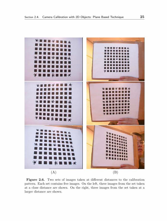
Figure 2.6. Two sets of images taken at different distances to the calibrationpattern. Each set contains five images. On the left, three images from the set takenat a close distance are shown. On the right, three images from the set taken at alarger distance are shown.


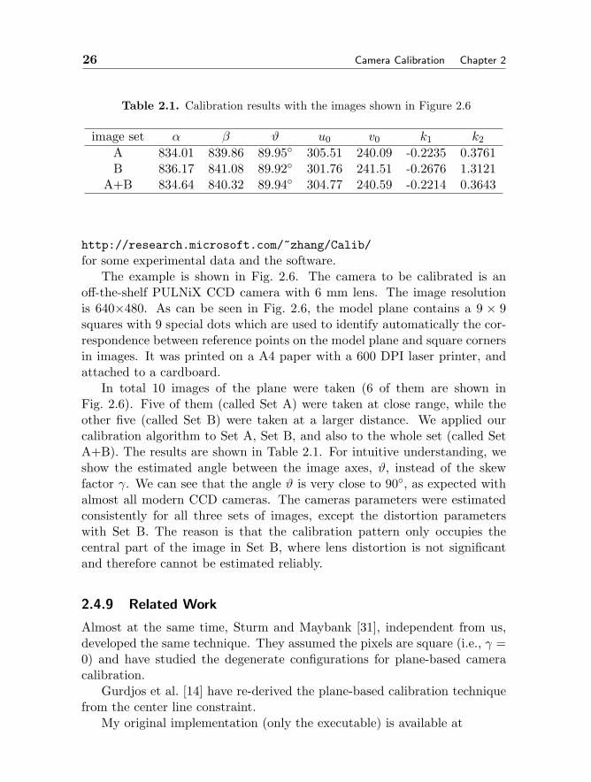
Table 2.1. Calibration results with the images shown in Figure 2.6

image set α β ϑ u0 v0 k1 k2

A 834.01 839.86 89.95 305.51 240.09 -0.2235 0.3761B 836.17 841.08 89.92 301.76 241.51 -0.2676 1.3121

A+B 834.64 840.32 89.94 304.77 240.59 -0.2214 0.3643

http://research.microsoft.com/˜zhang/Calib/for some experimental data and the software.

The example is shown in Fig. 2.6. The camera to be calibrated is anoff-the-shelf PULNiX CCD camera with 6 mm lens. The image resolutionis 640×480. As can be seen in Fig. 2.6, the model plane contains a 9 × 9squares with 9 special dots which are used to identify automatically the cor-respondence between reference points on the model plane and square cornersin images. It was printed on a A4 paper with a 600 DPI laser printer, andattached to a cardboard.

In total 10 images of the plane were taken (6 of them are shown inFig. 2.6). Five of them (called Set A) were taken at close range, while theother five (called Set B) were taken at a larger distance. We applied ourcalibration algorithm to Set A, Set B, and also to the whole set (called SetA+B). The results are shown in Table 2.1. For intuitive understanding, weshow the estimated angle between the image axes, ϑ, instead of the skewfactor γ. We can see that the angle ϑ is very close to 90, as expected withalmost all modern CCD cameras. The cameras parameters were estimatedconsistently for all three sets of images, except the distortion parameterswith Set B. The reason is that the calibration pattern only occupies thecentral part of the image in Set B, where lens distortion is not significantand therefore cannot be estimated reliably.

2.4.9 Related Work

Almost at the same time, Sturm and Maybank [31], independent from us,developed the same technique. They assumed the pixels are square (i.e., γ =0) and have studied the degenerate configurations for plane-based cameracalibration.

Gurdjos et al. [14] have re-derived the plane-based calibration techniquefrom the center line constraint.

My original implementation (only the executable) is available at

Section 2.5. Solving Camera Calibration With 1D Objects 27

http://research.microsoft.com/˜zhang/calib/.Bouguet has re-implemented my technique in Matlab, which is available athttp://www.vision.caltech.edu/bouguetj/calib doc/.

In many applications such as stereo, multiple cameras need to be cali-brated simultaneously in order to determine the relative geometry betweencameras. In 2000, I have extended (not published) this plane-based techniqueto stereo calibration for my stereo-based gaze-correction project [40, 39].The formulation is similar to (2.29). Consider two cameras, and denote thequantity related to the second camera by ′. Let (Rs, ts) be the rigid trans-formation between the two cameras such that (R′, t′) = (R, t) (Rs, ts) ormore precisely: R′ = RRs and t′ = Rts + t. Stereo calibration is then tosolve A,A′, k1, k2, k

′1, k

′2, (Ri, ti)|i = 1, . . . , n, and (Rs, ts) by minimizing

the following functional:

n∑i=1

m∑j=1

[δij‖mij − m(A, k1, k2,Ri, ti, Mj)‖2 + δ′

ij‖m′ij − m(A′, k′

1, k′2,R

′i, t

′i, Mj)‖2

](2.30)

subject toR′i = RiRs and t′

i = Rits + ti .

In the above formulation, δij = 1 if point j is visible in the first camera,and δij = 0 otherwise. Similarly, δ′

ij = 1 if point j is visible in the secondcamera. This formulation thus does not require the same number of featurepoints to be visible over time or across cameras. Another advantage of thisformulation is that the number of extrinsic parameters to be estimated hasbeen reduced from 12n if the two cameras are calibrated independently to6n+ 6. This is a reduction of 24 dimensions in parameter space if 5 planesare used.

Obviously, this is a nonlinear optimization problem. To obtain the ini-tial guess, we run first single-camera calibration independently for each cam-era, and compute Rs through SVD from R′

i = RiRs (i = 1, . . . , n) and tsthrough least-squares from t′

i = Rits + ti (i = 1, . . . , n). Recently, a closed-form initialization technique through factorization of homography matricesis proposed in [34].

2.5 Solving Camera Calibration With 1D Objects

In this section, we describe in detail how to solve the camera calibrationproblem from a number of observations of a 1D object consisting of 3 collinearpoints moving around one of them [43, 44]. We only consider this minimal


configuration, but it is straightforward to extend the result if a calibrationobject has four or more collinear points.

2.5.1 Setups With Free-Moving 1D Calibration Objects

We now examine possible setups with 1D objects for camera calibration.As already mentioned in the introduction, we need to have several observa-tions of the 1D objects. Without loss of generality, we choose the cameracoordinate system to define the 1D objects; therefore, R = I and t = 0 in(2.1).

Two points with known distance. This could be the two endpoints of a stick,and we take a number of images while waving freely the stick. Let A and Bbe the two 3D points, and a and b be the observed image points. Becausethe distance between A and B is known, we only need 5 parameters to defineA and B. For example, we need 3 parameters to specify the coordinates of Ain the camera coordinate system, and 2 parameters to define the orientationof the line AB. On the other hand, each image point provides two equationsaccording to (2.1), giving in total 4 equations. Given N observations ofthe stick, we have 5 intrinsic parameters and 5N parameters for the pointpositions to estimate, i.e., the total number of unknowns is 5+5N . However,we only have 4N equations. Camera calibration is thus impossible.

Three collinear points with known distances. By adding an additional point,say C, the number of unknowns for the point positions still remains thesame, i.e., 5 + 5N , because of known distances of C to A and B. For eachobservation, we have three image points, yielding in total 6N equations.Calibration seems to be plausible, but is in fact not. This is because thethree image points for each observation must be collinear. Collinearity ispreserved by perspective projection. We therefore only have 5 independentequations for each observation. The total number of independent equations,5N , is always smaller than the number of unknowns. Camera calibration isstill impossible.

Four or more collinear points with known distances. As seen above, when thenumber of points increases from two to three, the number of independentequations (constraints) increases by one for each observation. If we havea fourth point, will we have in total 6N independent equations? If so, wewould be able to solve the problem because the number of unknowns remainsthe same, i.e., 5 + 5N , and we would have more than enough constraints ifN ≥ 5. The reality is that the addition of the fourth point or even morepoints does not increase the number of independent equations. It will always


be 5N for any four or more collinear points. This is because the cross ratio ispreserved under perspective projection. With known cross ratios and threecollinear points, whether they are in space or in images, other points aredetermined exactly.

2.5.2 Setups With 1D Calibration Objects Moving Around a fixedPoint

From the above discussion, calibration is impossible with a free moving 1Dcalibration object, no matter how many points on the object. Now let usexamine what happens if one point is fixed. In the sequel, without loss ofgenerality, point A is the fixed point, and a is the corresponding image point.We need 3 parameters, which are unknown, to specify the coordinates of Ain the camera coordinate system, while image point a provides two scalarequations according to (2.1).

Two points with known distance. They could be the endpoints of a stick,and we move the stick around the endpoint that is fixed. Let B be the freeendpoint and b, its corresponding image point. For each observation, weneed 2 parameters to define the orientation of the line AB and therefore theposition of B because the distance between A and B is known. Given Nobservations of the stick, we have 5 intrinsic parameters, 3 parameters for Aand 2N parameters for the free endpoint positions to estimate, i.e., the totalnumber of unknowns is 8 + 2N . However, each observation of b providestwo equations, so together with a we only have in total 2 + 2N equations.Camera calibration is thus impossible.

Three collinear points with known distances. As already explained in the lastsubsection, by adding an additional point, say C, the number of unknownsfor the point positions still remains the same, i.e., 8+2N . For each observa-tion, b provides two equations, but c only provides one additional equationbecause of the collinearity of a, b and c. Thus, the total number of equationsis 2 + 3N for N observations. By counting the numbers, we see that if wehave 6 or more observations, we should be able to solve camera calibration,and this is the case as we shall show in the next section.

Four or more collinear points with known distances. Again, as already ex-plained in the last subsection, The number of unknowns and the number ofindependent equations remain the same because of invariance of cross-ratios.This said, the more collinear points we have, the more accurate camera cal-ibration will be in practice because data redundancy can combat the noisein image data.


2.5.3 Basic Equations

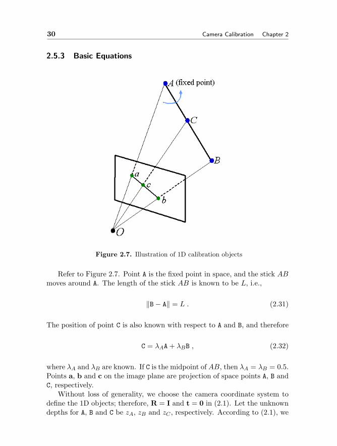
Figure 2.7. Illustration of 1D calibration objects

Refer to Figure 2.7. Point A is the fixed point in space, and the stick ABmoves around A. The length of the stick AB is known to be L, i.e.,

‖B− A‖ = L . (2.31)

The position of point C is also known with respect to A and B, and therefore

C = λAA + λBB , (2.32)

where λA and λB are known. If C is the midpoint of AB, then λA = λB = 0.5.Points a, b and c on the image plane are projection of space points A, B andC, respectively.

Without loss of generality, we choose the camera coordinate system todefine the 1D objects; therefore, R = I and t = 0 in (2.1). Let the unknowndepths for A, B and C be zA, zB and zC , respectively. According to (2.1), we


have

A = zAA−1a (2.33)

B = zBA−1b (2.34)

C = zCA−1c . (2.35)

Substituting them into (2.32) yields

zC c = zAλAa + zBλBb (2.36)

after eliminating A−1 from both sides. By performing cross-product on bothsides of the above equation with c, we have

zAλA(a× c) + zBλB(b× c) = 0 .

In turn, we obtain

zB = −zA λA(a× c) · (b× c)

λB(b× c) · (b× c). (2.37)

From (2.31), we have

‖A−1(zBb− zAa)‖ = L .

Substituting zB by (2.37) gives

zA‖A−1(a +λA(a× c) · (b× c)

λB(b× c) · (b× c)b)‖ = L .

This is equivalent toz2AhTA−TA−1h = L2 (2.38)

with

h = a +λA(a× c) · (b× c)

λB(b× c) · (b× c)b . (2.39)

Equation (2.38) contains the unknown intrinsic parameters A and the un-known depth, zA, of the fixed point A. It is the basic constraint for cameracalibration with 1D objects. Vector h, given by (2.39), can be computed fromimage points and known λA and λB. Since the total number of unknownsis 6, we need at least six observations of the 1D object for calibration. Notethat A−TA actually describes the image of the absolute conic [20].


2.5.4 Closed-Form Solution

Let

B = A−TA−1 ≡B11 B12 B13B12 B22 B23B13 B23 B33

(2.40)

=

1α2 − γ

α2βv0γ−u0βα2β

− γα2β

γ2

α2β2 + 1β2 −γ(v0γ−u0β)

α2β2 − v0β2

v0γ−u0βα2β

−γ(v0γ−u0β)α2β2 − v0

β2(v0γ−u0β)2

α2β2 + v20β2 +1

. (2.41)

Note that B is symmetric, and can be defined by a 6D vector

b = [B11, B12, B22, B13, B23, B33]T . (2.42)

Let h = [h1, h2, h3]T , and x = z2Ab, then equation (2.38) becomes

vTx = L2 (2.43)

withv = [h2

1, 2h1h2, h22, 2h1h3, 2h2h3, h

23]T .

When N images of the 1D object are observed, by stacking n such equationsas (2.43) we have

Vx = L21 , (2.44)

where V = [v1, . . . ,vN ]T and 1 = [1, . . . , 1]T . The least-squares solution isthen given by

x = L2(VTV)−1VT1 . (2.45)

Once x is estimated, we can compute all the unknowns based on x = z2Ab.

Let x = [x1, x2, . . . , x6]T . Without difficulty, we can uniquely extract theintrinsic parameters and the depth zA as

v0 = (x2x4 − x1x5)/(x1x3 − x22)

zA =√x6 − [x2

4 + v0(x2x4 − x1x5)]/x1

α =√zA/x1

β =√zAx1/(x1x3 − x2

2)

γ = −x2α2β/zA

u0 = γv0/α− x4α2/zA .

At this point, we can compute zB according to (2.37), so points A andB can be computed from (2.33) and (2.34), while point C can be computedaccording to (2.32).


2.5.5 Nonlinear Optimization


We are given N images of the 1D calibration object and there are 3points on the object. Point A is fixed, and points B and C moves around A.Assume that the image points are corrupted by independent and identicallydistributed noise. The maximum likelihood estimate can be obtained byminimizing the following functional:

N∑i=1

(‖ai − φ(A, A)‖2 + ‖bi − φ(A, Bi)‖2 + ‖ci − φ(A, Ci)‖2), (2.46)

where φ(A, M) (M ∈ A, Bi, Ci) is the projection of point M onto the image,according to equations (2.33) to (2.35). More precisely, φ(A, M) = 1

zMAM,

where zM is the z-component of M.The unknowns to be estimated are:

– 5 camera intrinsic parameters α, β, γ, u0 and v0 that define matrix A;

– 3 parameters for the coordinates of the fixed point A;

– 2N additional parameters to define points Bi and Ci at each instant(see below for more details).

Therefore, we have in total 8 + 2N unknowns. Regarding the parameteri-zation for B and C, we use the spherical coordinates φ and θ to define thedirection of the 1D calibration object, and point B is then given by

B = A + L

sin θ cosφsin θ sinφ

cos θ

where L is the known distance between A and B. In turn, point C is computedaccording to (2.32). We therefore only need 2 additional parameters for eachobservation.

Minimizing (2.46) is a nonlinear minimization problem, which is solvedwith the Levenberg-Marquardt Algorithm as implemented in Minpack [23].It requires an initial guess of A, A, Bi, Ci|i = 1..N which can be obtainedusing the technique described in the last subsection.


2.5.6 Estimating the fixed point

In the above discussion, we assumed that the image coordinates, a, of thefixed point A are known. We now describe how to estimate a by consideringwhether the fixed point A is visible in the image or not.

Invisible fixed point. The fixed point does not need to be visible in the image.And the camera calibration technique becomes more versatile without thevisibility requirement. In that case, we can for example hang a string ofsmall balls from the ceiling, and calibrate multiple cameras in the room byswinging the string. The fixed point can be estimated by intersecting linesfrom different images as described below.

Each observation of the 1D object defines an image line. An image linecan be represented by a 3D vector l = [l1, l2, l3]T , defined up to a scale factorsuch as a point m = [u, v]T on the line satisfies lT m = 0. In the sequel, wealso use (n, q) to denote line l, where n = [l1, l2]T and q = l3. To removethe scale ambiguity, we normalize l such that ‖l‖ = 1. Furthermore, each lis associated with an uncertainty measure represented by a 3× 3 covariancematrix Λ.

GivenN images of the 1D object, we haveN lines: (li,Λi)|i = 1, . . . , N.Let the fixed point be a in the image. Obviously, if there is no noise, wehave lTi a = 0, or nTi a + qi = 0. Therefore, we can estimate a by minimizing

F =N∑i=1

wi‖lTi a‖2 =N∑i=1

wi‖nTi a + qi‖2 =N∑i=1

wi(aTninTi a + 2qinTi a + q2i )

(2.47)where wi is a weighting factor (see below). By setting the derivative of Fwith respect to a to 0, we obtain the solution, which is given by

a = −( N∑i=1

wininTi)−1( N∑

i=1

wiqini).

The optimal weighting factor wi in (2.47) is the inverse of the variance of lTi a,which is wi = 1/(aTΛia). Note that the weight wi involves the unknown a.To overcome this difficulty, we can approximate wi by 1/ trace(Λi) for thefirst iteration, and by re-computing wi with the previously estimated a inthe subsequent iterations. Usually two or three iterations are enough.

Visible fixed point. Since the fixed point is visible, we have N observations:ai|i = 1, . . . , N. We can therefore estimate a by minimizing

∑Ni=1 ‖a−ai‖2,

assuming that the image points are detected with the same accuracy. Thesolution is simply a = (

∑Ni=1 ai)/N .


The above estimation does not make use of the fact that the fixed pointis also the intersection of the N observed lines of the 1D object. Therefore,a better technique to estimate a is to minimize the following function:

F =N∑i=1

[(a−ai)TV−1

i (a−ai)+wi‖lTi a‖2]

=N∑i=1

[(a−ai)TV−1

i (a−ai)+wi‖nTi a+qi‖2]

(2.48)where Vi is the covariance matrix of the detected point ai. The derivativeof the above function with respect to a is given by

∂F∂a

= 2N∑i=1

[V−1i (a− ai) + wininTi a + wiqini

].

Setting it to 0 yields

a =( N∑i=1

(V−1i + wininTi )

)−1( N∑i=1

(V−1i ai − wiqini)

).

If more than three points are visible in each image, the known cross ratioprovides an additional constraint in determining the fixed point.

For an accessible description of uncertainty manipulation, the reader isreferred to [45, Chapter 2].

2.5.7 Experimental Results

The proposed algorithm has been tested on both computer simulated dataand real data.

Computer Simulations

The simulated camera has the following property: α = 1000, β = 1000,γ = 0, u0 = 320, and v0 = 240. The image resolution is 640×480. A stick of70 cm is simulated with the fixed point A at [0, 35, 150]T . The other endpointof the stick is B, and C is located at the half way between A and B. We havegenerated 100 random orientations of the stick by sampling θ in [π/6, 5π/6]and φ in [π, 2π] according to uniform distribution. Points A, B, and C arethen projected onto the image.

Gaussian noise with 0 mean and σ standard deviation is added to theprojected image points a, b and c. The estimated camera parameters arecompared with the ground truth, and we measure their relative errors withrespect to the focal length α. Note that we measure the relative errors in


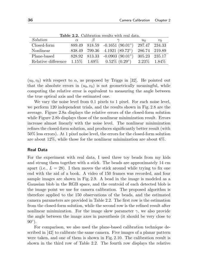
Table 2.2. Calibration results with real data.Solution α β γ u0 v0Closed-form 889.49 818.59 -0.1651 (90.01) 297.47 234.33Nonlinear 838.49 799.36 4.1921 (89.72) 286.74 219.89Plane-based 828.92 813.33 -0.0903 (90.01) 305.23 235.17Relative difference 1.15% 1.69% 0.52% (0.29) 2.23% 1.84%

(u0, v0) with respect to α, as proposed by Triggs in [32]. He pointed outthat the absolute errors in (u0, v0) is not geometrically meaningful, whilecomputing the relative error is equivalent to measuring the angle betweenthe true optical axis and the estimated one.

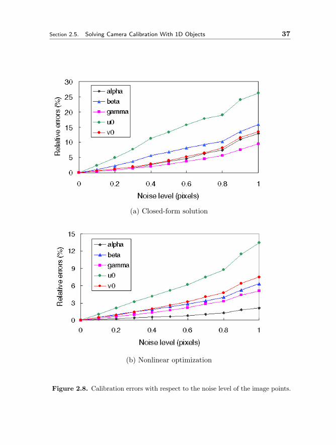
We vary the noise level from 0.1 pixels to 1 pixel. For each noise level,we perform 120 independent trials, and the results shown in Fig. 2.8 are theaverage. Figure 2.8a displays the relative errors of the closed-form solutionwhile Figure 2.8b displays those of the nonlinear minimization result. Errorsincrease almost linearly with the noise level. The nonlinear minimizationrefines the closed-form solution, and produces significantly better result (with50% less errors). At 1 pixel noise level, the errors for the closed-form solutionare about 12%, while those for the nonlinear minimization are about 6%.

Real Data

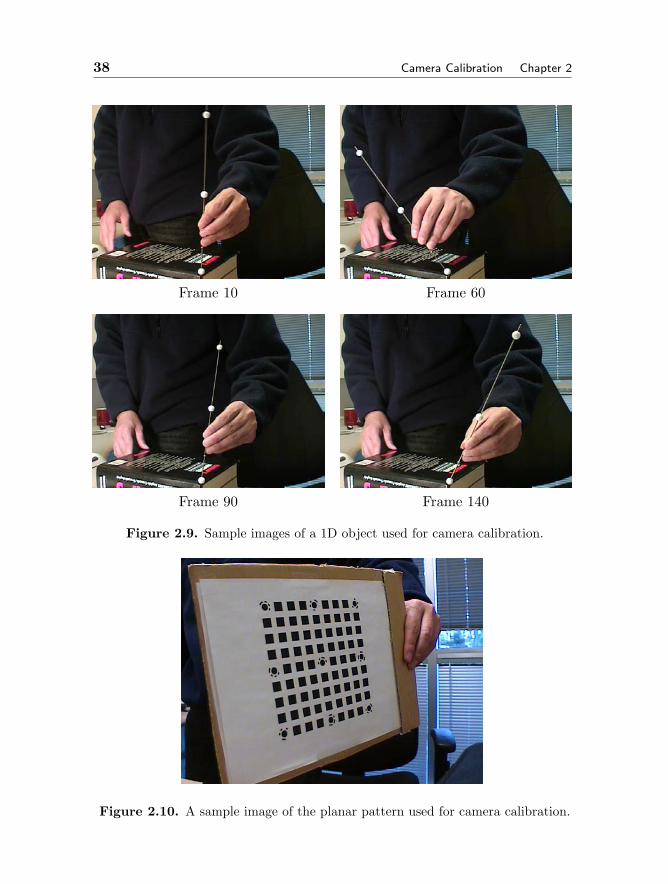
For the experiment with real data, I used three toy beads from my kidsand strung them together with a stick. The beads are approximately 14 cmapart (i.e., L = 28). I then moves the stick around while trying to fix oneend with the aid of a book. A video of 150 frames was recorded, and foursample images are shown in Fig. 2.9. A bead in the image is modeled as aGaussian blob in the RGB space, and the centroid of each detected blob isthe image point we use for camera calibration. The proposed algorithm istherefore applied to the 150 observations of the beads, and the estimatedcamera parameters are provided in Table 2.2. The first row is the estimationfrom the closed-form solution, while the second row is the refined result afternonlinear minimization. For the image skew parameter γ, we also providethe angle between the image axes in parenthesis (it should be very close to90).

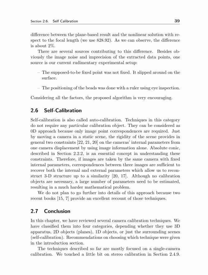
For comparison, we also used the plane-based calibration technique de-scribed in [42] to calibrate the same camera. Five images of a planar patternwere taken, and one of them is shown in Fig. 2.10. The calibration result isshown in the third row of Table 2.2. The fourth row displays the relative


(a) Closed-form solution

(b) Nonlinear optimization

Figure 2.8. Calibration errors with respect to the noise level of the image points.


Frame 10 Frame 60

Frame 90 Frame 140

Figure 2.9. Sample images of a 1D object used for camera calibration.

Figure 2.10. A sample image of the planar pattern used for camera calibration.

Section 2.6. Self Calibration 39

difference between the plane-based result and the nonlinear solution with re-spect to the focal length (we use 828.92). As we can observe, the differenceis about 2%.

There are several sources contributing to this difference. Besides ob-viously the image noise and imprecision of the extracted data points, onesource is our current rudimentary experimental setup:

– The supposed-to-be fixed point was not fixed. It slipped around on thesurface.

– The positioning of the beads was done with a ruler using eye inspection.

Considering all the factors, the proposed algorithm is very encouraging.

2.6 Self-Calibration

Self-calibration is also called auto-calibration. Techniques in this categorydo not require any particular calibration object. They can be considered as0D approach because only image point correspondences are required. Justby moving a camera in a static scene, the rigidity of the scene provides ingeneral two constraints [22, 21, 20] on the cameras’ internal parameters fromone camera displacement by using image information alone. Absolute conic,described in Section 2.2.2, is an essential concept in understanding theseconstraints. Therefore, if images are taken by the same camera with fixedinternal parameters, correspondences between three images are sufficient torecover both the internal and external parameters which allow us to recon-struct 3-D structure up to a similarity [20, 17]. Although no calibrationobjects are necessary, a large number of parameters need to be estimated,resulting in a much harder mathematical problem.

We do not plan to go further into details of this approach because tworecent books [15, 7] provide an excellent recount of those techniques.

2.7 Conclusion

In this chapter, we have reviewed several camera calibration techniques. Wehave classified them into four categories, depending whether they use 3Dapparatus, 2D objects (planes), 1D objects, or just the surrounding scenes(self-calibration). Recommendations on choosing which technique were givenin the introduction section.

The techniques described so far are mostly focused on a single-cameracalibration. We touched a little bit on stereo calibration in Section 2.4.9.


Camera calibration is still an active research area because more and moreapplications use cameras. In [2], spheres are used to calibrate one or morecameras, which can be considered as a 2D approach since only the surfaceproperty is used. In [5], a technique is described to calibrate a camera net-work consisting of an omni-camera and a number of perspective cameras. In[24], a technique is proposed to calibrate a projector-screen-camera system.

2.8 Appendix: Estimating Homography Between the ModelPlane and its Image

There are many ways to estimate the homography between the model planeand its image. Here, we present a technique based on maximum likelihoodcriterion. Let Mi and mi be the model and image points, respectively. Ideally,they should satisfy (2.18). In practice, they don’t because of noise in theextracted image points. Let’s assume that mi is corrupted by Gaussian noisewith mean 0 and covariance matrix Λmi . Then, the maximum likelihoodestimation of H is obtained by minimizing the following functional∑

i

(mi − mi)TΛ−1mi

(mi − mi) ,

where mi =1

hT3 Mi

[hT1 MihT2 Mi

]with hi, the ith row of H.

In practice, we simply assume Λmi = σ2I for all i. This is reasonable if pointsare extracted independently with the same procedure. In this case, the aboveproblem becomes a nonlinear least-squares one, i.e., minH

∑i ‖mi − mi‖2.

The nonlinear minimization is conducted with the Levenberg-Marquardt Al-gorithm as implemented in Minpack [23]. This requires an initial guess,which can be obtained as follows.

Let x = [hT1 , hT2 , h

T3 ]T . Then equation (2.18) can be rewritten as[

MT 0T −uMT0T MT −vMT

]x = 0 .

When we are given n points, we have n above equations, which can be writtenin matrix equation as Lx = 0, where L is a 2n×9 matrix. As x is defined upto a scale factor, the solution is well known to be the right singular vector ofL associated with the smallest singular value (or equivalently, the eigenvectorof LTL associated with the smallest eigenvalue). In L, some elements areconstant 1, some are in pixels, some are in world coordinates, and some aremultiplication of both. This makes L poorly conditioned numerically. Muchbetter results can be obtained by performing a simple data normalizationprior to running the above procedure.

Bibliography 41

Bibliography

[1] Y.I. Abdel-Aziz and H.M. Karara. Direct linear transformation into objectspace coordinates in close-range photogrammetry. In Proceedings of the Sym-posium on Close-Range Photogrammetry, University of Illinois at Urbana-Champaign, Urbana, Illinois, pages 1–18, January 1971.

[2] M. Agrawal and L. Davis. Camera calibration using spheres: A semi-definiteprogramming approach. In Proceedings of the 9th International Conference onComputer Vision, pages 782–789, Nice, France, October 2003. IEEE ComputerSociety Press.

[3] D. C. Brown. Close-range camera calibration. Photogrammetric Engineering,37(8):855–866, 1971.

[4] B. Caprile and V. Torre. Using Vanishing Points for Camera Calibration. TheInternational Journal of Computer Vision, 4(2):127–140, March 1990.

[5] X. Chen, J. Yang, and A. Waibel. Calibration of a hybrid camera network.In Proceedings of the 9th International Conference on Computer Vision, pages150–155, Nice, France, October 2003. IEEE Computer Society Press.

[6] W. Faig. Calibration of close-range photogrammetry systems: Mathematicalformulation. Photogrammetric Engineering and Remote Sensing, 41(12):1479–1486, 1975.

[7] O. Faugeras and Q.-T. Luong. The Geometry of Multiple Images. The MITPress, 2001. With contributions from T. Papadopoulo.

[8] O. Faugeras. Three-Dimensional Computer Vision: a Geometric Viewpoint.MIT Press, 1993.

[9] O. Faugeras, T. Luong, and S. Maybank. Camera self-calibration: theory andexperiments. In G. Sandini, editor, Proc 2nd ECCV, volume 588 of LectureNotes in Computer Science, pages 321–334, Santa Margherita Ligure, Italy,May 1992. Springer-Verlag.

[10] O. Faugeras and G. Toscani. The calibration problem for stereo. In Proceedingsof the IEEE Conference on Computer Vision and Pattern Recognition, pages15–20, Miami Beach, FL, June 1986. IEEE.

[11] S. Ganapathy. Decomposition of transformation matrices for robot vision. Pat-tern Recognition Letters, 2:401–412, December 1984.

[12] D. Gennery. Stereo-camera calibration. In Proceedings of the 10th Image Un-derstanding Workshop, pages 101–108, 1979.

[13] G.H. Golub and C.F. van Loan. Matrix Computations. The John HopkinsUniversity Press, Baltimore, Maryland, 3 edition, 1996.

[14] P. Gurdjos, A. Crouzil, and R. Payrissat. Another way of looking at plane-basedcalibration: the centre circle constraint. In Proceedings of the 7th EuropeanConference on Computer Vision, volume IV, pages 252–266, Copenhagen, May2002.

[15] R. Hartley and A. Zisserman. Multiple View Geometry in Computer Vision.Cambridge University Press, 2000.

[16] R. Hartley. Self-calibration from multiple views with a rotating camera. In J-O. Eklundh, editor, Proceedings of the 3rd European Conference on ComputerVision, volume 800-801 of Lecture Notes in Computer Science, pages 471–478,Stockholm, Sweden, May 1994. Springer-Verlag.


[17] R. Hartley. An algorithm for self calibration from several views. In Proceedingsof the IEEE Conference on Computer Vision and Pattern Recognition, pages908–912, Seattle, WA, June 1994. IEEE.

[18] J. Heikkila and O. Silven. A four-step camera calibration procedure with im-plicit image correction. In Proceedings of the IEEE Conference on ComputerVision and Pattern Recognition, pages 1106–1112, San Juan, Puerto Rico, June1997. IEEE Computer Society.

[19] D. Liebowitz and A. Zisserman. Metric rectification for perspective images ofplanes. In Proceedings of the IEEE Conference on Computer Vision and Pat-tern Recognition, pages 482–488, Santa Barbara, California, June 1998. IEEEComputer Society.

[20] Q.-T. Luong and O.D. Faugeras. Self-calibration of a moving camera frompoint correspondences and fundamental matrices. The International Journal ofComputer Vision, 22(3):261–289, 1997.

[21] Q.-T. Luong. Matrice Fondamentale et Calibration Visuelle surl’Environnement-Vers une plus grande autonomie des systemes robotiques.PhD thesis, Universite de Paris-Sud, Centre d’Orsay, December 1992.

[22] S. J. Maybank and O. D. Faugeras. A theory of self-calibration of a movingcamera. The International Journal of Computer Vision, 8(2):123–152, August1992.

[23] J.J. More. The levenberg-marquardt algorithm, implementation and theory. InG. A. Watson, editor, Numerical Analysis, Lecture Notes in Mathematics 630.Springer-Verlag, 1977.

[24] T. Okatani and K. Deguchi. Autocalibration of projector-screen-camera sys-tem: Theory and algorithm for screen-to-camera homography estimation. InProceedings of the 9th International Conference on Computer Vision, pages774–781, Nice, France, October 2003. IEEE Computer Society Press.

[25] L. Robert. Camera calibration without feature extraction. Computer Vision,Graphics, and Image Processing, 63(2):314–325, March 1995. also INRIA Tech-nical Report 2204.

[26] J.G. Semple and G.T. Kneebone. Algebraic Projective Geometry. Oxford:Clarendon Press, 1952. Reprinted 1979.

[27] S.W. Shih, Y.P. Hung, and W.S. Lin. Accurate linear technique for cameracalibration considering lens distortion by solving an eigenvalue problem. OpticalEngineering, 32(1):138–149, 1993.

[28] I. Shimizu, Z. Zhang, S. Akamatsu, and K. Deguchi. Head pose determina-tion from one image using a generic model. In Proceedings of the IEEE ThirdInternational Conference on Automatic Face and Gesture Recognition, pages100–105, Nara, Japan, April 1998.

[29] C. C. Slama, editor. Manual of Photogrammetry. American Society of Pho-togrammetry, fourth edition, 1980.

[30] G. Stein. Accurate internal camera calibration using rotation, with analysis ofsources of error. In Proc. Fifth International Conference on Computer Vision,pages 230–236, Cambridge, Massachusetts, June 1995.

Bibliography 43

[31] P. Sturm and S. Maybank. On plane-based camera calibration: A generalalgorithm, singularities, applications. In Proceedings of the IEEE Conferenceon Computer Vision and Pattern Recognition, pages 432–437, Fort Collins,Colorado, June 1999. IEEE Computer Society Press.

[32] B. Triggs. Autocalibration from planar scenes. In Proceedings of the 5th Euro-pean Conference on Computer Vision, pages 89–105, Freiburg, Germany, June1998.

[33] R. Y. Tsai. A versatile camera calibration technique for high-accuracy 3D ma-chine vision metrology using off-the-shelf tv cameras and lenses. IEEE Journalof Robotics and Automation, 3(4):323–344, August 1987.

[34] T. Ueshiba and F. Tomita. Plane-based calibration algorithm for multi-camerasystems via factorization of homography matrices. In Proceedings of the 9thInternational Conference on Computer Vision, pages 966–973, Nice, France,October 2003. IEEE Computer Society Press.

[35] G.Q. Wei and S.D. Ma. A complete two-plane camera calibration methodand experimental comparisons. In Proc. Fourth International Conference onComputer Vision, pages 439–446, Berlin, May 1993.

[36] G.Q. Wei and S.D. Ma. Implicit and explicit camera calibration: Theory andexperiments. IEEE Transactions on Pattern Analysis and Machine Intelligence,16(5):469–480, 1994.

[37] J. Weng, P. Cohen, and M. Herniou. Camera calibration with distortion modelsand accuracy evaluation. IEEE Transactions on Pattern Analysis and MachineIntelligence, 14(10):965–980, October 1992.

[38] R. Willson. Modeling and Calibration of Automated Zoom Lenses. PhD thesis,Department of Electrical and Computer Engineering, Carnegie Mellon Univer-sity, 1994.

[39] R. Yang and Z. Zhang. Eye gaze correction with stereovision for video tele-conferencing. In Proceedings of the 7th European Conference on ComputerVision, volume II, pages 479–494, Copenhagen, May 2002. Also available asTechnical Report MSR-TR-01-119.

[40] R. Yang and Z. Zhang. Model-based head pose tracking with stereovision.In Proc. Fifth IEEE International Conference on Automatic Face and GestureRecognition (FG2002), pages 255–260, Washington, DC, May 2002. Also avail-able as Technical Report MSR-TR-01-102.

[41] Z. Zhang. A flexible new technique for camera calibration. Technical ReportMSR-TR-98-71, Microsoft Research, December 1998. Available together withthe software at http://research.microsoft.com/˜zhang/Calib/.

[42] Z. Zhang. A flexible new technique for camera calibration. IEEE Transactionson Pattern Analysis and Machine Intelligence, 22(11):1330–1334, 2000.

[43] Z. Zhang. Camera calibration with one-dimensional objects. Technical ReportMSR-TR-2001-120, Microsoft Research, December 2001.

[44] Z. Zhang. Camera calibration with one-dimensional objects. In Proc. Euro-pean Conference on Computer Vision (ECCV’02), volume IV, pages 161–174,Copenhagen, Denmark, May 2002.

[45] Z. Zhang and O.D. Faugeras. 3D Dynamic Scene Analysis: A Stereo BasedApproach. Springer, Berlin, Heidelberg, 1992.

CAMERA CALIBRATION - Computer Science calibration is a necessary step in 3D computer vision in order...

Documents

Transcript of CAMERA CALIBRATION - Computer Science calibration is a necessary step in 3D computer vision in order...