NBER WORKING PAPER SERIES

THE DYNAMIC EFFECTS OF AGGREGATE DEMAND AND SUPPLY DISTURBANCES

Olivier Jean Blanchard

Danny Quah

Working Paper No. 2737

NATIONAL BUREAU OF ECONOMIC RESEARCH1050 Massachusetts Avenue

Cambridge, MA 02138October 1988

Both authors are with the Economics Department, MIT, and the NBER. We thankStanley Fischer, Julio Rotemberg, Mark Watson for helpful discussions, andthe NSF for financial assistance. We are also grateful for the comments oftwo anonymous referees and of participants at an NBER Economic Fluctuationsmeeting, and for the hospitality of the MIT Statistics Center. This researchis part of the NBER's research program in Economic Fluctuations. Anyopinions expressed are those of the authors not those of the National Bureauof Economic Research.

NBER Working Paper #2737October 1988

THE DYNAMIC EFFECTS OF AGGREGATE DEMAND AND SUPPLY DISTURBANCES

ABSTRACT

We interpret fluctuations in GNP and unemployment as due to two types ofdisturbances: distur-

bances that have a permanent effect on output and disturbance.s that do not. We interpret the first

as supply disturbances, the second as demand disturbances.

We find that demand disturbances have a hump shaped effect on both output and unem ploy-

ment; the effect peaks after a year and vanishes after two to five years. Up to a scale factor, the

dynamic effect on unemployment of demand disturbances is a mirror image of that on output. The

effect of supply disturbances on output increases steadily over time, to reach a peak after two years

and a plateau after five years. 'Favorab1e supply disturbances may initially increase unem ploy-

ment. This is followed by a decline in unemployment, with a slow return over time to its original

value.

While this dynamic characterization is fairly sharp, the data are not as specific as to the relative

contributions of demand and supply disturbances to output fluctuations. We find that the time

series of demand-determined output fluctuations has peaks and troughs which coincide with most

of the NBER troughs and peaks. But variance decompositions of output at various horizons giving

the respective contributions of supply and demand disturbances are not precisely estimated. For

instance, at a forecast horizon of four quarters, we find that, under alternative assumptions, the

contribution of demand disturbances ranges from 40 to over 95 per cent.

Olivier Jean Blanchard Danny QuahDepartment of Economics Department of EconomicsMIT MITCambridge, MA 02139 Cambridge, MA 02139

1

Introduction.

It is now widely accepted that GNP is reasonably characterized as a unit root process: a positive innovation in

CNP should lead one to revise upwards one's forecast of GNP for all horizons. Following the influential work

of Nelson and Plosser (1982), this statistical characterization has been recorded and refined by numerous

authors including Campbell and Mankiw (1987a), Clark (1987a, b), Cochrane (1988), Diebold and Rudebusch

(1987), Evans (1987), and Watson (1986).

How should this finding affect one's views about macroeconomic fluctuations? Were there only one

type of disturbance in the economy, then the implications of these findings would be straightforward. That

disturbance would affect the economy in a way characterized by estimated univariate moving average rep-

resentations, such as those given by Campbell and Mankiw. The problem would simply be to find out what

this disturbance was, and why its dynamic effects had the shape that they did. The way to proceed would

be clear.

However, if GNP is affected by more than one type of disturbance, as is likely, the interpretation becomes

more difficult. In that case, the univariate moving average representation of output is some combination

of the dynamic response of output to each of the disturbances. The work in Beveridge and Nelson (1981),

Harvey (1985) and Watson (1986) can be viewed as early attempts to get at this issue.'

To proceed, given the possibility that output may be affected by more than one type of disturbance,

one can impose a priori restrictions on the response of output to each of the disturbances, or one can exploit

information from macroeconomic variables other than GNP. In addition to the work named above, Clark

(1987a) has also used the first approach. This paper adopts the second, and considers the joint behavior

of output and unemployment. Campbell and Mankiw (1987b), Clark (1987b), and Evans (1987) have also

taken this approach. Our analysis differs mainly in its choice of identifying restrictions; as we shall argue,

we find our restrictions more appealing than theirs.

Our approach is conceptually straightforward. We assume that there are two kinds of disturbances, each

As will become clear, our work differs from these in that we wish to examine the dynamic effectsof disturbances that have permanent effects; such issues cannot be addressed by studies that restrict thepermanent component to be a random walk. In other work, one of us has characterized the effects of differentparametric specifications (such as lag length restrictions, a rational form for the lag distribution) for thequestion of the relative importance of permanent and transitory components. See Quah (1988).

2

uncorrelated with the other, and that neither has a long run effect on unemployment. We assume howeve;

that the first has a long run effect on output while the second does not. These assumptions are sufficient t

just identify the two types of disturbances, and their dynamic effects on output and unemployment.

While the disturbances are defined by the identification restrictions, we believe that they can be giver

a simple economic interpretation. Namely, we interpret the disturbances that have a temporary effect or

output as being mostly demand disturbances, and those that have a permanent effect on output as mostly

supply disturbances. We present a simple model in which this interpretation is warranted and use it tc

discuss the justification for, as well as the limitations of, this interpretation.

Under these identification restrictions and this economic interpretation, we obtain the following charac-

terization of fluctuations: demand disturbances have a hump shaped effect on both output and unemploy-

ment; the effect peaks after a year and vanishes after two to three years. Up to a scale factor, the dynamic

effect on unemployment of demand disturbances is a mirror image of that on output. The effect of supply

disturbances on output increases steadily over time, to reach a peak after two years and a plateau after five

years. uFavorable supply disturbances may initially increase unemployment. This is followed by a decline

in unemployment, with a slow return over time to its original value.

While this dynamic characterization is fairly sharp, the data are not as specific as to the relative

contributions of demand and supply disturbances to output fluctuations. On the one hand, we find that

the time series of demand-determined output fluctuations, that is the time series of output constructed by

putting all supply disturbance realizations equal to zero, has peaks and troughs which coincide with most of

the NBER troughs and peaks. But, when we turn to variance decompositions of output at various horizons,

we find that the respective contributions of supply and demand disturbances are not precisely estimated. For

instance, at a forecast horizon of four quarters, we find that, under alternative assumptions, the contribution

of demand disturbances ranges from 40% to over 95%.

The rest of the paper is organized as follows. Section 1 analyzes identification, and Section 2 discusses

our economic interpretation of the disturbances. Section 3 discusses estimation, and Section 4 characterizes

the dynamic effects of demand and supply disturbances on output and unemployment. Section 5 characterizes

the relative contributions of demand and supply disturbances to fluctuations in output and unemployment.

3

1. Identification.

In this section, we show how our assumptions characterize the process followed by output and unemployment,

and how this process can be recovered from the data.

We make the following assumptions. There are two types of disturbances affecting unemployment and

output. The first has no long run effect on either unemployment or output. The second has no long run effect

on unemployment, but may have a long run effect on output. Finally, these twodisturbances are uncorrelated

at all leads and lags. These restrictions in effect define the two disturbances. As indicated in the Introduction,

and discussed at length in the next section, we will refer to the first as demand disturbances, and to the

second as supply disturbances. How we name the disturbances however is irrelevant for the argument of this

section.

We now derive the joint process followed by output and unemployment implied by our assumptions.

Let Y and U denote the logarithm of GNP and the level of the unemployment rate, respectively, and let Cd

and e be the two disturbances. Let X be the vector (iY, U)' and e be the vector of disturbances (Cd,e,)'.

The assumptions above imply that X follows a stationary process given by:

X(t) = A(O)e(t) + A(1)e(t — 1) + -• - = > A(j)e(t — i). Var(e) = 1 (1.1)j=0

where the sequence of matrices A is such that its upper left hand entry, ajj(j), y = 1,2, ..., sums to zero.

Equation (1.1) gives Y and U as distributed lags of the two disturbances, Cd and e1. Since these two

disturbances are assumed to be uncorrelated, their variance covariance matrix is diagonal; the assumption

that the covariance matrix is the identity is then simply a convenient normalization. The contemporaneous

effect of e on X is given by A(O); subsequent lag effects are given by A(j), � 1. As X has been assumed

to be stationary, neither disturbance has a long run effect on either unemployment, U, or the rate of change

in output, Y. The restriction a11(;) = 0 implies that Cd also has no effect on the level of Y itself.

To see why this is, notice that aii(j) is the effect of d Ofl Y afterj periods, and therefore, E-..-0aji() is

the effect of c,g on 1' itself after k periods. For Cd to have no effect on Y in the long run, we mu•st havethen

that E0 aii&) = 0.

We now show how to recover this representation from the data. Since X is stationary, it has a Wold

4

moving average representation:

X(t) ii(t) + C(1)v(t — 1) +. = CU)v(t — j), Var(v) = a (i.1=0

This moving average representation is unique and can be obtained by first estimating and then inverting ti

vector autoregressive representation of X in the usual way.

Comparing equations (1.1) and (1.2), we see that v, the vector of innovations, and e, the vector

original disturbances, are related by v = A(O)e, and that A(j) = C(j)A(O), for all . Thus knowledge

A(O) allows one to recover e from z.', and similarly to obtain A(j) from C(j).

Is A(O) identified? An informal argument suggests that it is. Equations (1.1) and (1.2) imply th

A(O) satisfies: A(O)A(O)' = Li, and that the upper left-hand entry in A(j) = (>I.o C(y)) A(o)

0. Given Li, the first relation imposes three restrictions on the four elements of A(O); given C(j

the other implication imposes a fourth restriction. This informal argument is indeed correct. A rigoroi

and constructive proof, which we actually use to obtain A(O) is as follows: Let S denote the unique lowe

triangular Choleski factor of Ii. Any matrix A(O) such that A(O)A(O)' =Li is an orthonormal transformatic

of S. The restriction that the upper left hand entry in C(,)) A(0) be equal to 0 is an orthogonalit

restriction that then uniquely determines this orthonormal transformation.2

In summary, our procedure is as follows. We first estimate a vector autoregressive representation for)

and invert it to obtain (1.2). We then construct the matrix A(0); and use this to obtain A(y) =C(j)A(O), j

0, 1,2,..., and Ct = A(O)&'. This gives output and unemployment as functions of current and past deman

and supply disturbances.

2 Notice that identification is achieved by a long-run restriction. This raises a knotty technical issuWithout precise prior knowledge of lag lengths, inference and restrictions on the kind of long-run behaviwe are interested in here is delicate. See for instance Sims (1972); we are extrapolating here from Simsresults which assume strictly exogenous regressors. Similar problems may arise in the VAR case, althouthe results of Berk (1974) suggest otherwise. Nevertheless, we can generalize our long run restriction to ojthat applies to some neighborhood of frequency zero, instead of just a restriction at the point zero. Undappropriate regularity conditions, we can show that our results are the limit of those from that kindrestriction, as the neighborhood shrinks to zero.

5

2. Interpretation.

Interpreting residuals in small dimensional systems as "structural" disturbances is always perilous, and our

interpretation of disturbances as supply and demand disturbances is no exception. We discuss various issues

in turn.

Our interpretation of disturbances with permanent effects as supply disturbances, and of disturbances

with transitory effects as demand disturbances is motivated by a traditional Keynesian view of fluctuations.

For illustrative purposes, as well as to focus the discussion below, we now provide a simple model which

delivers those implications. The model is a variant of Fischer (1977):

Y(t) = ?vf(t) — P(t) + a 0(t) (2.1)

Y(t) = N(t) + 0(t) (2.2)

P(t) = W(t) — 0(t) (2.3)

W(t) = W {E_1N(t) = N} (2.4)

The variables Y, N, and 0 denote the log of output, employment, and productivity respectively. Full

employment is represented by N; and P, W, and M are the log of the price level, the nominal wage, and

the money supply.

Equation (2.1) states that aggregate demand is a function of real balances and productivity. Notice

that productivity is allowed to affect aggregate demand directly; it can do so through investment demand

for example, in which case a > 0. Equation (2.2) is the production function: it relates output, employment

and productivity, and assumes a constant returns to scale technology. Equation (2.3) describes price setting

behavior, and gives the price level as a function of the nominal wage and of productivity. Finally the

last equation, (2.4), characterizes wage setting behavior in the economy: the wage is chosen one period in

advance, and is set so as to achieve (expected) full employment.

To close the model, we need to specify how M and 0 evolve. We assume that they follow:

M(t) = M(t — 1) + ed(t) (2.5)

9(t) = 0(t — 1) + e.(t) (2.6)

6

where e,j and e are the serially uncorrelated and pairwise orthogonal demand and supply disturbances

Define unemployment U to be N — N; solving for unemployment and output growth then gives:

Y =ed(t) — ed(t — 1) + a (ea(t) — e,(t — 1)) + e8(t)

U = —ed(t) — a e,(t)

These two equations clearly satisfy the restrictions in equation (1.1) of the previous section. Due to nomina

rigidities, demand disturbances have short run effects on output and unemployment, but these effects disap

pear over time. In the long run, only supply, i.e. productivity disturbances here, affect output. Neither o

the disturbances have a long run impact on unemployment.

This model is clearly only illustrative. More complex wage and price dynamics, such as in Taylo

(1980), will also satisfy the long run properties embodied in equation (1.1). This model is nevertheless

useful vehicle to discuss the limitations of our interpretation of permanent and transitory disturbances.

Granting our interpretation of these disturbances as demand and supply disturbances, one may never

theless question the assumption that the two disturbances are uncorrelated at all leads and lags. We thin

of this as a non-issue. The model makes clear that this orthogonality assumption does not eliminate fo

example the possibility that supply disturbances directly affect aggregate demand. Put another way, th.

assumption that the two disturbances are uncorrelated does not restrict the channels through which demanc

and supply disturbances affect output and unemployment.

Again granting our interpretation of these disturbances as demand and supply disturbances, one ma)

argue that even demand disturbances have a long run impact on output: changes in the subjective discount

rate, or changes in fiscal policy may well affect the savings rate, and subsequently the long run capital stoci

and output. The presence of increasing returns, and of learning by doing, also raise the possibility tha

demand disturbances may have some long run effects. Even if not, their effects through capital accumulatioi

may be sufficiently long lasting as to be indistinguishable from truly permanent effects in a finite data sample

We agree that demand disturbances may well have such long run effects on output. However, we also beiev

that if so, those long run effects are small compared to those of supply disturbances. To the extent that thi

is true then, our decomposition is "nearly correct" in the following sense: in a sequence of economies wher

the size of the long run effect of demand disturbances becomes arbitrarily small relative to that of supply

7

the correct identifying scheme approaches that which we actually use. This result is proven in the technical

appendix.

This raises a final set of issues, one inherent in the estimation and interpretation of any low dimensional

dynamic system. It is likely that there are in fact many sources of disturbances, each with different dynamic

effects on output and on unemployment, rather than only two as we assume here. Certainly if there are

many supply disturbances, some with permanent and others with transitory effects on output, together with

many demand disturbances, some with permanent and others with transitory effects, and if they all play

an equally important role in aggregate fluctuations, our decomposition is likely to be meaningless. A more

interesting case is that where all the supply disturbances have permanent output effects, and where all the

demand disturbances have only transitory output effects. One may then hope that, in this case, what we

present as "the" demand shock represents an average of the dynamic effects of the different shocks (in the

sense of Granger and Morris (1976) for example), and similarly for supply shocks. This however is not true

in general: a simple counter-example that illustrates this is provided in the Technical Appendix. However,

we also present in the Appendix necessary and sufficient conditions such that an aggregation proposition

does hold. Those conditions will be satisfied if for instance, the economy is subject to only one supply

disturbance but many demand disturbances, where each of the demand disturbances has different dynamic

effects on output, but all the demand disturbances leave unaffected the dynamic relation between output

and unemployment. That demand disturbances should leave the relation between output and unemployment

nearly unaffected is highly plausible. That the economy is subject to only one, or at least to one dominant,

source of supply disturbances is more questionable. If there are many supply disturbances of roughly equal

importance, and if, as is likely, each of them affects the dynamic relation between unemployment and output,

our decomposition is likely to be meaningless.

In summary, our interpretation of the disturbances is subject to various caveats. Nevertheless we believe

that interpretation to be reasonable and useful in understanding the results below. We now briefly discuss

the relation of our paper to others on the same topic. We first examine how our approach relates to the

business-cycle-versus_trend distinction.

Following estimation, we can construct two output series, a series reflecting only the effects of supply

8

disturbances, obtained by setting all realizations of the demand disturbances to zero, and a series reflectin1

only the effects of demand disturbances, obtained by setting supply realizations to zero. By construction, th

first series, the supply component of output, will be non-stationary while the second, the demand component

is stationary.3

A standard distinction in describing output movements is the "business cycle versus trend" distinction

While there is no standard definition of these components, the trend is usually taken to be that part of output

that would realize, were all prices perfectly flexible; business cycles are then taken to be the dynamics o

actual output around its trend.4

It is tempting to associate the first series we construct with the "trend" component of output and the

second series with the "business cycle" component. In our view, that association is unwarranted, If prices

are in fact imperfectly flexible, deviations from trend will arise not only from demand disturbances, but

also from supply disturbances: business cycles will occur due to both supply and demand disturbances. Pu

another way, supply disturbances will affect both the business cycle and the trend component. Identifyin

separately business cycles and trend is likely to be difficult, as the two will be correlated through their joint

dependence on current and past supply disturbances.

With this discussion in mind, we now review the approaches to identification used by others.

Campbell and Mankiw (1987b) assume the existence of two types of disturbances, "trend" and "cycle'

disturbances, which are assumed to be uncorrelated. Their identifying restriction is then that trend distur-

bances do not affect unemployment. The discussion above suggests that this assumption of zero correlatior

between cycle and trend components is unattractive; if their two disturbances are instead reinterpreted a.

supply and demand disturbances respectively, the identifying restriction that supply disturbances do not

affect unemployment is equally unattractive.

There is a technical subtlety here: strictly speaking, the fact that the sum of coefficients approaches zeris a necessary but not sufficient condition for the demand component to be stationary. However it turns outto be sufficient when unemployment and output growth are individually ARMA processes. This is provetin Quah (1988).

A precise definition would obviously be tricky but is not needed for our argument. In models witimperfect information, this would be the path of output, absent imperfect information. In models witinominal rigidities, this would be the path of output, absent nominal rigidities. In models that assumemarket clearing and perfect information, such as Prescott (1987), the distinction between business cycleand trend is not a useful one.

9

Clark (1987b) also assumes the existence of "trend" and "cycle" disturbances, and also assumes that

"trend" disturbances do not affect unemployment but allows for contemporaneous correlation between trend

and cycle disturbances. While this may be seen as an improvement over CarnpbeU and Mankiw, it still

severely constrains the dynamic effects of disturbances on output and unemployment in ways that are

difficult to interpret.

The paper closest to ours is that of Evans (1987). Evans assumes two disturbances, "unemployment"

and "output" disturbances, which can be reinterpreted as supply and demand disturbances respectively. By

assuming the existence of a reduced form identical to equation (1.2) above, he also assumes that neither

supply nor demand disturbances have a long run effect on unemployment, but that both may have a long

run effect on the level of output. However, instead of using the long run restriction that we use here, he

assumes that supply disturbances have no contemporaneous effect on output. We find this restriction less

appealing as a way of achieving identification; it should be clear however that our paper builds on Evans'

work.

3. Estimation.

We need to confront one final problem before estimation. The representation we use in Section 1 assumes

that both the level of unemployment and the first difference of the logarithm of GNP are stationary around

given levels. Postwar US data however suggest instead both a small but steady increase in the average

unemployment rate over the sample, as well as a decline in the average growth rate of GNP since the

mid-1970's.5 This raises two issues.

The first is that our basic assumptions may be wrong in fundamental ways. For instance, unemployment

might in fact be nonstationary, and affected even in the long run by demand and supply disturbances. This

is predicted by models with a "hysteresis" effect, as developed in Blanchard and Summers (1986), and used

by them to explain European unemployment. This property also obtains in some recent growth models

with increasing returns to scale, where changes in the savings rate may affect not only the level but also

The increase in the unemployment rate, sometimes attributed to demographic changes, is evident evenin the relatively homeogenous labor group on which we focus our attention. We use the seasonally adjustedunemployment rate for Males, age 20 and over. This is from Labor Force Statistics derived from the CurrentPopulation Survey, volume 2, US Department of Labor, Bureau of Labor Statistics, September 1982, andfrom Table A-39, Employment and Earnings, February issues.

10

the growth rate of output. While we cannot claim that such effects are not present here, we are willing to

assume that their importance is minimal, for the period and the economy at hand.

Next, there is the issue of how to handle the apparent time trend in unemployment, and the apparent

slowdown in growth since the mid-1970's. There is no clean solution for this, and we take an eclectic

approach.6 To focus the discussion, we present as a base case the results from estimation allowing for a

change in the growth rate of output, and for a secular increase in the unemployment rate, as captured by a

fitted linear time trend regression line. There are three other cases of interest: (A) there is no change in the

growth rate of output, but there is a secular change in the unemployment rate; (B) there is no secular trend

in the unemployment rate, but there is a break in the average growth rate of output; and finally, (C) there

is neither a change in the growth rate of output nor a secular change in the unemployment rate.

A VAR system in real GNP growth (tY) and the unemployment rate (U), allowing for eight lags

is estimated using observations from 1950:2 through 1987:4. The GNP data are quarterly; the monthly

unemployment data are averaged to provide quarterly observations. Evans (1987) has estimated essentially

the same bivariate VAR representation, although he uses instead the aggregate civilian unemployment rate.

He has also tested the stationarity assumptions that we use here. The properties of the VAR representation

and of the moving average representation found by direct inversion do not have any meaning within our

framework, so we do not discuss those further here.

The mean growth rates for output are 3.62% and 2.43%, at an annual rate, over 1948:2 through 1973:4,

and 1974:1 through 1987:4 respectively. This break point is chosen to coincide with the first OPEC oil shock.

The fitted time trend regression coefficient for the unemployment rate series is 0.019, which implies a secular

increase of 2.97 percentage points over the sample period. When we allow for a change in the output growth,

we simply remove the different sample means before estimating the vector autoregression; similarly when we

allow for a secular change in the unemployment rate, the fitted trend line is removed before VAR analysis.

It turns out that the results for cases (A)_(C) are qualitatively similar to those for the base case. More

6 See for example Perron (1987) and Christiano(1988) on the statistical evidence for and against a breakin average growth over the post War period.

Estimation with twelve lags produced little difference in the results. We also experimented with omittingthe first five years, as the Korean War experience seemed anomalous. Again, the empirical results remainpractically unchanged.

'Iprecisely, the moving average responses to demand and supply disturbances are sufficiently close to those

of the base case in their main features; the principal differences lie in the magnitudes of the responses.

These differences are notable only in forecast error variance decompositions; we will therefore present four

such decomposition tables for the different cases below. Because of the similarity in the other qualitative

features however, and to conserve space, we will present results for the impulse responses and historical

decompositions only for the base case.8

We turn next to the dynamic effects of demand and supply disturbances.

4. Dynamic effects of demand and supply disturbances.

The dynamic effects of demand and supply disturbances are reported in Figures 1 and 2. The vertical axes in

Figures 1 and 2 denote simultaneously the log of output and the rate of unemployment; the horizontal axis

denotes time in quarters. Figures 3-6 provide the same information, but now with one standard deviation

bands around the point estimates.9

Demand disturbances have a hump shaped effect on output and unemployment. Their effects peak after

two to four quarters. The effects of demand then decline to vanish after about three to five years. The

responses in output and unemployment are mirror images of each other; we return to this aspect of the

results below after discussing the effects of supply disturbances.

The output response is smallest when the raw data are used, without allowing for a break or a secular

change in unemployment (case C, not plotted); it also decays the most rapidly in this case. Once a change

in the average growth rate of output is allowed, the treatment of possible secular changes in unemployment

seems to be relatively unimportant for the responses to demand disturbances.

These dynamic effects are consistent with a traditional view of the dynamic effects of aggregate demand

on output and unemployment, in which movements in aggregate demand build up until the adjustment of

prices and wages leads the economy back to equilibrium.

8 The other graphs are available from the authors upon request.More precisely, these boundaries are separated from the point estimate by the square root of mean

squared deviations in each direction, over 1000 bootstrap replications. Thus the bands need not be andindeed are not symmetric. By construction, they will of course necessarily include the point estimate. Ineach case, pseudo-histories are created by drawing with replacement from the empirical distribution of theVAR innovations.

Figure 1

1.40

1.20 Response to Demand

1.00

0.80

0.60

0.40I — output

Unemployment

0.20

0.00

0 10 20 30 40-0.20

.040

.0.60

Figure 2

Response to Supply

1.00

0.80

0.60

0.40

0.20

0.00

-0.20 -

-0.40 -

-0.60 -

20

— Output

Unemployment

30 40

1.40

1.20

1.00

0.80

0.60

0.40

0.20

0.00

-0.20 1

Figure 3

Output Response to Demand

10 20 30 40

1.40

1.20

1.00

0.80

0.60

0.40

0.20

0.00

0'

-0.20 1.

Figure 4

Output Response to Supply

10 20 30 40

0.10

0.00

-0.10

-0.20

-0.30

-0.40

-0.50

-0.60

Figure 5

Unemployment Response to Demand

30 40

0.50

0.40

0.30

0.20

0.10

0.00

-0.10

-0.20

Figure 6

40

Unemployment Response to Supply

30

12

Supply disturbances have an effect on the level of output which cumulates steadily over time. In the

base case, the peak response is about eight times the initial effect and takes place after eight quarters.

The effect decreases to stabilize eventually. For good statistical reasons, the long-run impact is imprecisely

estimated. The dynamic response in unemployment is quite different: a positive supply disturbance (.that is,

a supply disturbance that has a positive long run effect on output) initially increases unemployment slightly.

Following this increase, the effect is reversed after a few quarters, and unemployment slowly returns to its

original steady state value. The dynamic effects of a supply disturbance on unemployment are largely over

by about five years.

The qualitative results are similar across all alternative treatments of breaks and time trends. The

oniy significant difference appears in the initial unemployment response to demand disturbances: in the case

when neither break nor time trend is permitted, the response is initially negative rather than positive as in

the base case. The one standard deviation band does however include positive values.

The response of unemployment and output are suggestive of the presence of rigidities, both nominal

and real. Nominal rigidities can explain why in response to a positive supply shock, say an increase in

productivity, aggregate demand does not initially increase enough to match the increase in output needed

to maintain constant unemployment; real wage rigidities can explain why increases in productivity can lead

to a decline in unemployment after a few quarters which persists until real wages have caught up with the

new higher level of productivity.

Figures 1 and 2 also shed an interesting light on the relation between changes in unemployment and

output known as Okun's law. The textbook value of Okun's coefficient is about 2.5. Under our interpretation,

this coefficient is a mongrel coefficient, as the joint behavior of output and unemployment depends on the

type of disturbance affecting the economy. In the case of demand disturbances, Figure 1 suggests that there

is indeed a tight relation between output and unemployment. At the peakresponses, the graph suggests a

implied coefficient between output and unemployment that is slightly greater than 2. In the case of supply

disturbances, there is no such close relation between output and unemployment. In the short run, output

increases, unemployment may rise or fall; in the long run, output remains higher whereas -by assumption-

unemployment returns to its initial value. In the intervening period, unemployment and output deviations

13

are of opposite sign. At the peak responses, Figure 2 suggests an implied coefficient slightly exceeding four,

higher in absolute value than Okun's coefficient. That the absolute value of the coefficient is higher for

supply disturbances than for demand disturbances is exactly what we expect. Supply disturbances are likely

to affect the relation between output and employment, and to increase output with little or no change in

employment.

5. Relative contributions of demand and supply disturbances.

Having shown the dynamic effects of each type of disturbance, the next step is to assess their relative

contribution to fluctuations in output and unemployment. We do this in two ways. The first is informal,

and entails a comparison of the historical time series of the demand component of output to the NBER

chronology of business cycles. The second examines variance decompositions of output and unemployment

in demand and supply disturbances at various horizons.

a. Demand disturbances and NBER business cycles.

From estimation of the joint process for output and unemployment, and our identifying restrictions, we

can form the "demand components" of output and unemployment. These are the time paths of output and

unemployment that would have obtained in the absence of supply disturbances. Similarly, by setting demand

innovations to zero, we can generate the time series of "supply components" in output and unemployment.

From the identifying restriction that demand disturbances have no long run effect on output, the resulting

series of the demand component in the level of output is stationary. By the same token, both the demand

and supply components of unemployment are stationary.

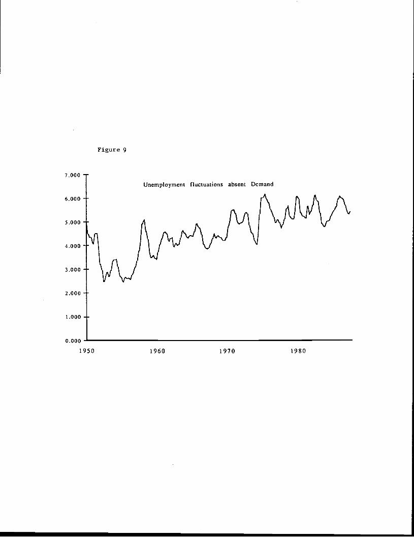
The time series for these components are presented in Figures 7 through 10. Superimposed on these

time series are the NBER peaks and troughs. Peaks are drawn as vertical lines above the horizontal a.xis,

troughs as vertical lines below the axis.

The peaks and troughs of the demand component in output match closely the NBER peaks and troughs.

The two recessions of 1974-1975 and 1979-1980 deserve special mention. Our decomposition attributes them

in about equal proportions to adverse supply and demand disturbances. This is best shown by giving the

estimated values of the supply and demand innovations over these periods. These are collected in Table

8.400

8.2 00

8.000

7.8 00

7.600

7.400

7.200

7.000

Figure 7

1950 1960 1970 1980

Output fluctuations absent Demand

0.100

0.080

0.060

0.040

0.020

0.000

-0.020

-0.040

-0.060

-0.080

-0.100

Figure 8

Output fluctuations due to Demand

1950 1960 1970 1980

7.000

6.000

5.000

4.000

3.000

2.000

1.000

0.000

Figure 9

1950 1960 1970 1980

Unemployment fluctuations absent Demand

Figure 10

Unemployment fluctuations due to Demand4.000

3.000

2.000

1.000

0.000

-1.000

-2.000

-3.000

-4.000

1950 1960 1970 1980

14

1. The recession of 1974-75 is therefore explained by an initial string of negative supply disturbances, and

then of negative demand disturbances. Similarly, the 1979-80 recession is first dominated by a large negative

supply disturbance in the second quarter of 1979, and then a large negative demand disturbance a year

later. Without appearing to interpret every single residual, we find these estimated sequences of demand

and supply disturbances consistent with less formal descriptions of these episodes.'°

Notice that the supply component in output, presented in Figure 7, is clearly not a deterministic trend.

It exhibits slower growth in the late 1950's, as well as in the 1970's.

Figures 9 and 10 give the supply and demand components in unemployment. Unemployment fluctuations

due to demand correspond closely to those in the demand component of GNP. This is consistent with our

earlier finding on the mirror image moving average responses of unemployment and output growth to demand

disturbances. The model attributes substantial fluctuation in unemployment to supply disturbances, again

with increases in the late 1950's and around the time of the oil disturbances of the 1970's.11

b. Variance decompositions.

While the above empirical evidence is suggestive, a more formal statistical assessment can be given by

computing variance decompositions for output and unemployment at various horizons.

Tables 2, and 2A.C give this variance decomposition for the different cases. The table has the following

interpretation. Define the k quarter-ahead forecast error in output as the difference between the actual value

of output and its forecast from equation (1.2) as of k quarters earlier. This forecast error is due to both

unanticipated demand and supply disturbances in the last k quarters. The number for output at horizon

k, k = 1,. .. ,40 gives the percentage of variance of the k-quarter ahead forecast error due to demand. The

contribution of supply, not reported, is given by one hundred minus that number. A similar interpretation

10 Formal evidence of a slightly different nature is also available. In Blanchardand Watson (1986), evidencefrom four time series is used to decompose fluctuations into supply and demand disturbances. There therecession of 1975 is attributed in roughly equal proportions to adverse demand and supply disturbances,that of 1980 mostly to demand disturbances. To see how much our characterizaton of the dynamic effectsof demand and supply disturbances depend on the 1973-76 episode, we reestimated the model, leaving out1973-1 to 1976-4. The estimated dynamic effects of both demand and supply disturbances were nearlyidentical to those described above.

By construction, the supply component of unemployment is close to actual unemployment for the firstfew observations in the sample. Thus, the large decrease from 1950 to 1952 in the supply component simplyreflects the actual movement in unemployment in this period. In light of this, we re-estimated the modelfrom 1955-2 through the end of our sample. We found little change in the empirical results.

Table 1: Demand and Supply Innovations, Base Case.

Quarter ed(%) ea(%)1973-3 -0.8 -1.91973-4 0.3 -0.41974-1 -0.7 -0.01974-2 0.5 -1.51974-3 -1.8 -1.01974-4 -0.7 1.11975-1 -1.5 2.8

1979-1 -0.5 -0.31979-2 -0.4 -1.71979-3 0.7 0.61979-4 -0.8 0.21980-1 0.2 2.01980-2 -3.2 1.9

Notes:

1. The identified innovations are obtained by applying the transformation of Section 1 to the fitted VARresiduals. By construction, the standard deviations of these innovations are equal to 1%.

2. The estimated innovations for the other cases follow the same pattern as above.

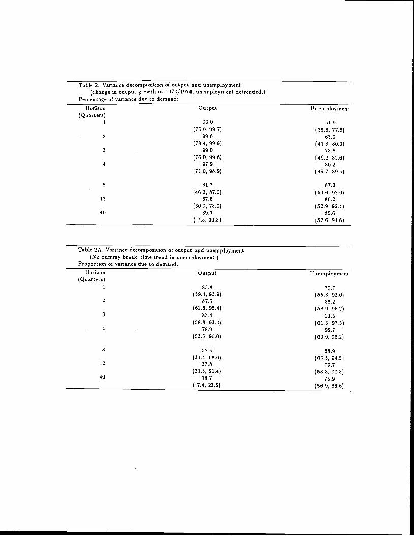
Table 2. Variance decomposition of output and unemployment(change in output growth at 1973/1974; unemployment detrended.)

Percentage of variance due to demand:

Horizon Output Unemployment(Quarters)

1 99.0 51.9(76.9, 99.7) (35.8, 77.6)

2 99.6 63.9(78.4, 99.9) (41.8, 80.3)

3 99.0 73.8(76.0, 99.6) (46.2, 85.6)

97.9 80.2(71.0, 98.9) (49.7, 89.5)

8 81.7 87.3

(46.3, 87.0) (53.6, 92.9)12 67.6 86.2

(30.9, 73.9) (52.9, 92.1)40 39.3 85.6

7.5, 39.3) (52.6, 91.6)

Table 2A. Variance decomposition of output and unemployment(No dummy break, time trend in unemployment.)

Proportion of variance due to demand:Horizon Output Unemployment

(Quarters)1 83.8 79.7

(59.4, 93.9) (55.3, 92.0)2 87.5 88.2

(62.8, 95.4) (58.9, 95.2)3 83.4 93.5

(58.8, 93.3) (61.3, 97.5)4 78.9 95.7

(53.5, 90.0) (63.9, 98.2)

8 52.5 88.9(31.4, 68.6) (63.5, 94.5)

12 37.8 79.7(21.3, 51.4) (58.8, 90.3)

40 18.7 75.9

_______________________________________ (7.4, 23.5) (56.9, 88.6)

Table 2B. Variance decomposition of output and unemployment(change in output growth at 1973/1974; no trend in unemployment.)

Percentage of variance due to demand:Horizon Output Unemployment

(Quarters)1 99.3 50.7

(75.0, 99.8) (32.0, 79.9)2 99.7 63.2

(77.6, 99.9) (36.6, 83.3)3 99.4 73.4

(76.1, 99.7) (40.8, 88.3)4 98.6 80.0

(72.9, 99.2) (44.3, 91.1)

8 86.3 88.4(53.2, 91.5) (50.0, 94.6)

12 75.5 88.9

(40.9, 83.0) (49.9, 94.6)40 50.4 90.0

(12.5, 54.8) (49.7, 95.0)

Table 2C. Variance decomposition of output and unemployment(No dummy break, no trend in unemployment.)

Proportion of variance due to demand:Horizon Output Unemployment

(Quarters)1 45.2 99.8

(20.1, 77.6) (76.6,100.0)2 50.2 98.3

(23.4, 79.9) (72.8, 99.3)3 44.2 92.7

(20.4, 77.0) (67.1, 97.8)4 38.9 85.9

(17.1, 72.7) (62.7, 95.8)

8 19.6 60.5( 8.8, 54.4) (44.3, 89.6)

12 12.9 47.6( 6.5, 43.5) (35.2, 87.8)

40 5.2 40.5( 2.4, 17.7) (31.4, 87.1)

15

holds for the numbers for unemployment. The numbers in parentheses are one standard deviation bands,

surrounding the point estimate.12

Our identifying restrictions impose only one restriction on the variance decompositions, namely that

the contribution of supply disturbances to the variance of output tends to unity as the horizon increases.

All other aspects are unconstrained.

Two principal conclusions emerge from these tables.

First, the data do not give a precise answer as to the relative contribution of demand and supply

disturbances to movements in output at short and medium term horizons. The results vary across alternative

treatments of break and trend. In the base case, the relative contribution of demand disturbances to output

fluctuations, at a four quarters horizon, is 98%. This contribution falls to 79% when no break is allowed

but there is a time trend in unemployment, remains about the same when a break is allowed in output

growth but there is no trend in the unemployment rate. When neither a break nor a trend is permitted,

it is only 39%. Next, the standard error bands are quite large in each case, ranging from 71% to 99% in

the base case, 54% to 90% in case A, 73% to 99% in case B, and 17% to in case C. Evidently when

a break is permitted in output growth, the treatment of the trend in unemployment appears to be quite

unimportant. These cases are also when the demand contribution is more precisely estimated. Despite the

differences across estimates, and the uncertainty associated with each set, we view the results as suggesting

an important role for demand disturbances in the short run.

Second, estimates of the relative contribution of the different disturbances to unemployment do not

appear to vary a great deal across alternative treatments of break and trend. The contribution of demand

disturbances, four quarters ahead, to unemployment fluctuations varies from 80% to 96%. In the base case,

the one standard error band ranges from 50% to 90% with a point estimate of 80%. In allcases, the demand

disturbance appears to be quite important for unemployment fluctuations at all horizons.

12 Again, these bands are asymmetric, and obtained as described above.

16

6. Conclusion and Extensions.

We have assumed the existence of two types of disturbances generating unemployment and output dynamics,

the first type having permanent effects on output, the second having only transitory effects. We have argued

that these two types of disturbances could usefully be interpreted as supply and demand shocks. Under

that interpretation, we have concluded that demand disturbances have a hump shaped effect on output and

unemployment which disappears after approximately two to three years, and that supply disturbances have

an effect on output which cumulates over time to reach a plateau after five years. We have also concluded

that demand disturbances make a substantial contribution to output fluctuations at short and medium term

horizons; however, the data do not allow us to quantify this contribution with great precision.

While we find this simple exercise to have been worthwhile, we also believe that further work is needed,

especially to validate and refine our identification of shocks as supply and demand shocks. We have in mind

two specific extensions. The first is to examine the co-movements of what we have labeled the demand and

supply components of GNP with a larger set of macroeconomic variables. Preliminary results appear to

confirm our interpretation of shocks. We find in particular the supply component of GNP to be positively

correlated with real wages at high to medium frequencies, while no such correlation emerges for the demand

component.'3 The second extension is to enlarge the system to one in four variables, unemployment, output,

prices and wages. This would re-examine the empirical questions in Blanchard (1986), by using the long run

identification restriction developed in this paper. This extension is important; one would expect that wage

and price data will help identify more explicitly supply and demand disturbances. Research by Gali (1988),

Jun (1988) and Shapiro and Watson (1988), has already extended our work in that particular direction.

' The methodology and results will be described in a future paper. The statement in the text refers tothe sum of correlations from lags .5 to +5 between the supply innovation derived in this paper and theinnovations in real wages obtained from univariate ARIMA estimation.

17

Technical Appendix

This technical appendix discusses further and establishes the claims made in the section on interpreta-

tion.

First, we asserted in the text that our identification scheme is approximately correct even when both

disturbances have permanent effects on the level of output, provided that the long-run effect of demand on

output is small. We now prove this.

The first element of the model, output growth, has the moving average representation in demand and

supply disturbances:

= ajj(L)edt + a12(L)e1g

where a11(1) is the cumulative effect on the level of output Y of the disturbance Cd. The moving average

representation C(L), together with the innovation covariance matrix ti, is related to our desired interpretable

representation through some identifying matrix S, such that:

55' = Il, and A(L) = C(L)S.

The model is identified by choosing a unique identifying matrix S. In the paper, we selected the unique

matrix S such that a11(1) = 0.

Let the long-run effect of the demand disturbance be 6 instead, where 6 >0 without loss of generality.

Foreach 6, this implies a different identifying matrix S(5). Let S(6) —5(0)1 =max,,k (S,(6) — S,k(0))2; this

measures the deviation in the implied identifying matrix from that which we use. Since the approximation

is thus seen to be a finite-dimensional problem, any matrix norm will induce the same topology, which is all

that is needed to study the continuity properties of our identification scheme. All of the empirical results

vary continuously in S relative to this topology. Thus, it is sufficient to show that

IS(6)—S(O)I—-O as6—.0.

In words, if an economy has long-run effects in demand that are small but different from zero, our identifying

scheme which incorrectly assumes the long-run effects to be icro nevertheless recovers approximately the

correct point estimates.

18

We prove this as follows. Since both 5(0) and S(5) are matrix square roots of Il, there exists an

orthogonal matrix V(5) such that:

S(5) = S(O)V(5), where V(5)V(6)' = I.

Then the long-run effect of demand is the (1, 1) element in the matrix:

A(l; 5) = C(1)S(5) = C(1)S(O)V(6).

But recall that the elements of the first row of C(1)S(O) are respectively, the long-run effects of demand

and of supply on the level of output, when the long-run effect of demand is restricted to be zero. Thus

for any V(5), the new implied long-run effect of demand is simply the long-run effect of supply (under our

identifying assumption that the long-run effect of demand is zero) multiplied by the (2, 2) element of the

orthogonal matrix V(5). As S tends to zero, the (2,2) element of V(5) tends continuously to zero as well.

But, up to a column sign change, the unique V(S) with (2,2) element equal to zero is the identity matrix.

This establishes that 5(5) —. S(O), element by element. Hence, we have shown that 15(5) — S(O)l — 0 as

5-.O. Q.E.D.

Next, we turn to the effects of multiple demand and supply disturbances: Suppose that there is a Pd x 1

vector of demand disturbances fdt, and a Pa x 1 vector of supply disturbances fat, so that:

(tY'\ — (B11(L)' B12(L)"\ (fatUt ) — '\B2l(L) B22(L)') fat

where B, are column vectors of analytic functions; B,1 has the same dimension as ía, B,2 has the same

dimension as f, and Bii(z) = (1 — z)9ij(z), for some vector of analytic functions jj. Each disturbance

has a different distributed lag effect on output and unemployment.

Since our VAR method allows identification of only as many disturbances as observed variables, it is

immediate that we will not be able to recover the individual components of I = (f, f)'.To clarify the issues involved, we provide an explicit example where our procedure produces misleading

results. Suppose that there is only one supply disturbance and two demand disturbances: fa = (fal,t, fd2,t)l.

Suppose further that the first demand disturbance affects only output, while the second demand disturbance

19

affects only unemployment. The supply disturbance affects both output and unemployment. Formally,

assume that the true model is:

1—L 0 1 (fdlt0 —1 1)Vd2tf&t

An unrestricted VAR representation corresponding to this data generating process is found by applying the

calculations in Rozanov (1965) Theorem 10.1 (pp. 44-48). The implied moving average representation is:

x= ( (2_L)) Er,tr=I.0

It is straightforward to verify that the matrix covariogram implied by this moving average matches that of

the true underlying model. Further, the unique zero of the determinant is 2, and consequently lies outside

the unit circle. Therefore this moving average representation is, as asserted, obtained from the vector

autoregressive representation of the true model.

However, this moving average does not satisfy our identifying assumption that the 'demand" disturbance

has only transitory effects on the level of output. We therefore apply our identifying transformation to obtain:

x= ((i_L) (3—L)" (cdt—1 1 J\e,t

This moving average representation is what we would recover ii in fact the data is generated by the three

disturbances (faj, fd2, fe). Notice that while the supply disturbance 1 affects both output growth and

unemployment equally and only contemporaneously, we would identify e1 to have a larger effect on output

than on unemployment, together with a distributed lag effect on output. Further a positive demand dis-

turbance, restricted to have only a transitory effect on output, is seen to have a contemporaneous negative

impact on unemployment. In the true model however, no demand disturbances affect output and unemploy-

ment together, either contemporaneously or at any lag. In conclusion, a researcher following our bivariate

procedure is likely to be seriously misled when in fact the true underlying model is driven by more than two

disturbances. Having seen this, we ask under what circumstances will this mismatch in the number of actual

and explicitly modeled disturbances be benign?

We state the necessary and sufficient conditions for this as a Theorem which is proved below.

20

Theorem: Let X be a bivariate stochastic sequence generated by

(i.) X = B(L)ft

(ii.) f=(f f)', withfdpdxl, f,p8xl;(iii.) Eft ft_a = I if k = 0, and 0 otherwise

I Bii(z)' B12(z)'(iv.) B(s)—

B2j(z) B22(z)

(v.) Bjj(z) = (1— z)f3ij(z)

(vi.) th1, B21, B12, B22 are column vectors of analytic functions; and B21 Pd x 1, B12 and B22 p. x I

(vii.) BB is full rank on Izi = 1, where * denotes complex conjugation followed by transposition.

Then there exists a bivariate moving average representation for X, X =A(L)e, such that:

(viii.) A(z) = (aui1 ai21), with a11, a12, a21, a22 scalar functions, det A 0 for all Izi � 1;

(ix.) a11(z) = (1— z)cxii(z), with a11 analytic on Izi� 1; and

= (edt) Eelet_k = I if k = 0, and is 0 otherwise.Cat

In the bivariate representation, Cd is orthogonal to f, and e is orthogonal to Id, at all leads and Ia

if and only if there exists a pair of scalar functions "yr, "12 such that:

B21 = - fiji,B22 = '72 B12.

Conditions (i.) - (vii.) describe the true data generating process for the observed data in output grow

and unemployment. There are Pd demand and p. supply disturbances; (v.) expresses the requirement th

demand disturbances have only transitory effects on the level of output. Condition (vii.) is a regulari

condition that allows the existence of a VAR mean square approximation. The moving average recover

by our VAR procedure is described by (viii.) - (x.): the Theorem guarantees that there always exists su

a representation.

The second part of the Theorem establishes necessary and sufficient conditions on the underlying moc

such that the bivariate identification procedure does not inappropriately confu8e demand and supply d

turbances. In words, correct identification is possible if and only if the individual distributed lag respont

21

in output growth and unemployment are sufficiently similar across the different demand disturbances, and

across the different supply disturbances. This does not mean that the dynamic responses in output growth

and unemployment across demand disturbances must be identical or proportional, simply that they differ

up to a scalar lag distribution.

Thus even though in general a bivariate procedure is misleading, there are important and reasonable

sets of circumstances under which our technique provides the correct" answers. For instance, suppose that

there is only one supply disturbance but multiple demand disturbances. Suppose further that each of the

demand components in the level of output has the same distributed lag relation with the corresponding

demand component in unemployment. This assumption is consistent with our production function"-based

interpretations below. Then our procedure correctly distinguishes the dynamic effects of demand and supply

components in output and unemployment.

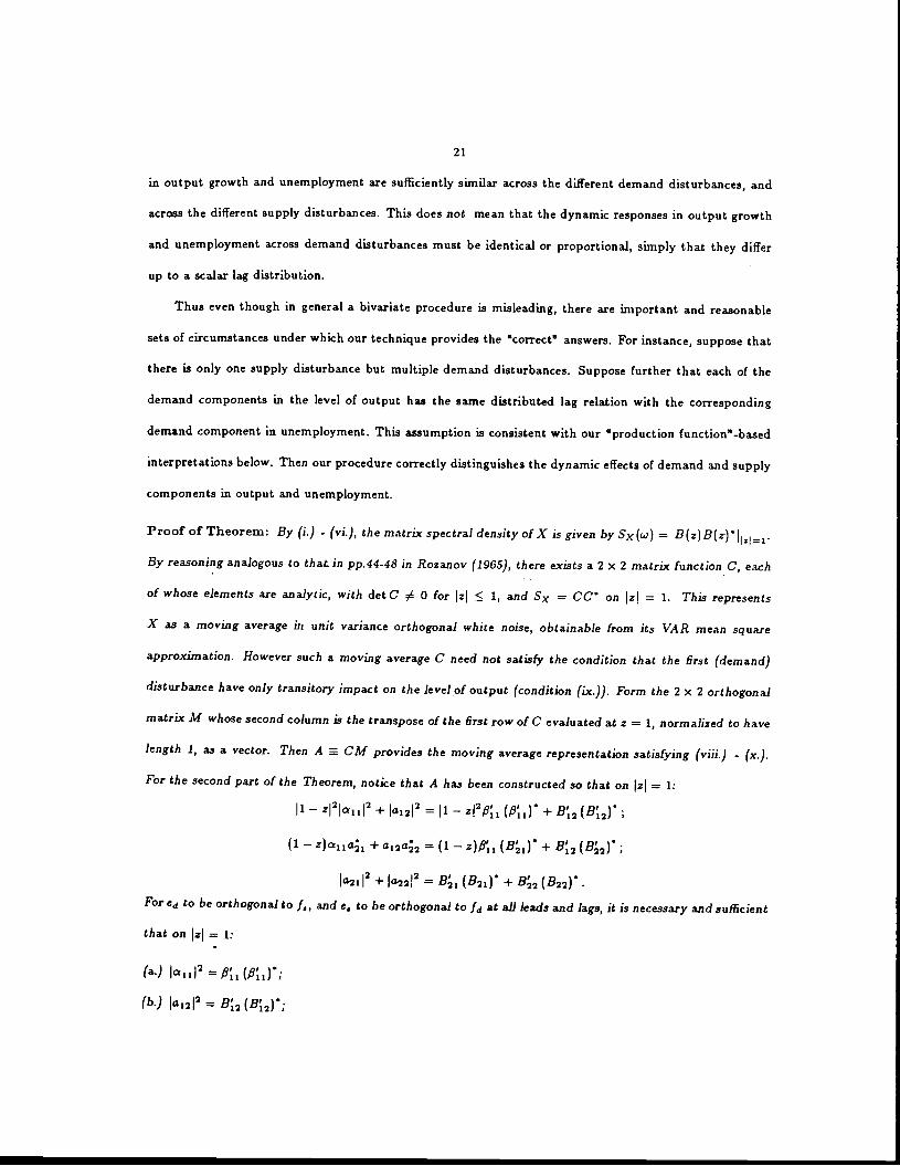
Proof of Theorem: By (i.) - (vi.), the matrix spectral density of X is given by Sx() = B(z)B(z-)'IIHl.

By reasoning analogous to that, in pp.44-48 in Rozanov (1965), there exists a 2 x 2 matrix function C, each

of whose elements are analytic, with det C 0 for zi < 1, and S = CC' on = 1. This represents

X as a moving average in unit variance orthogonal white noise, obtainable from its VAR mean square

approximation. However such a moving average C need not satisfy the condition that the first (demand)

disturbance have only transitory impact on the level of output (condition (ix.)). Form the 2 x 2 orthogonal

matrix M whose second column is the transpose of the first row of C evaluated at z =1, normalized to have

length 1, as a vector. Then A CM provides the moving average representation satisfying (viii.) - (x.).

For the second part of the Theorem, notice that A has been constructed so that on IzI = 1:

1— z2o112+ a1212 = 1 — zf2 (fi',) + B'12 (B'12)'

(1 — z)cxiia;1 + 0120;2 = (1 —z)1 (B1)' + B'12 (B2)'

071 2 + a222 = B1 (B21)' + B2 (B22)'.

Fore to be orthogonal to f, and e1 to be orthogonal to ía at all leads and lags, it is necessary and sufficient

that on zi = 1:

(a.) 1o12 fil (fi11)•;

(b.) 101212 = B'12 (B'12)';

22

(c.) ciia = I9 (B1) ;I_Il • DS lot'u., a12a22 — 12 t22

I 1 2_OS iD' .e.1 a21 — 21 21In 2_os in,a22 — 22t 22

Consider relations (a.), (c.), and (e.). Denoting complex conjugation of B by B, the triangle inequali

implies that:

flu B211 = f>13115B1,.I � IthijBI,

where the inequality is strict unless B21 is a complex scalar multiple of flu for each z on Izi= 1. Next,

the Cauchy.Schwarz inequality,

/ \1/2 / \1/2> flu, B111 � (E I/3uiI2) ( IBzuiI)

again with strict inequality except when B21 is a complex scalar multiple of fiji, for each z on =

Therefore:

Iiia2 � .I2 a22j2, on IzI = 1,

where the inequality is strict except when B21 is a complex scalar multiple of fl on Izi = 1. But t

strict inequality is a contradiction as and a22 are just scalar functions. Thus (a.), (c.), and (e.) can I

simultaneously satisfied if and only if there exists some complex scalar function 'yj(z) such that B21 = 'Yi th

A similar argument applied to (b.), (d.), and (f.) shows that they can hold simultaneously if and only

there exists some complex scalar function '72(z) such that B22 = '72 B12. This establishes the Theorei

Q.E.D.

23

References

Berk, K.N., "Consistent Autoregressive Spectral Estimates," Annals of Statistics, 1974, 2 no.3, 489-502.

Blanchard, Olivier, "Wages, Prices, and Output: An Empirical Investigation," mimeo MIT, 1986.

Blanchard Olivier and Lawrence Summers, "Hysteresis and European Unemployment", MacroeconomicsAnnual, 1986, 15-78.

Blanchard, Olivier and Mark Watson, "Are business cycles all alike?" in "The American business cycle;continuity and change", R. Gordon ed, NBER and University of Chicago Press, 1986, 123-156.

Campbell, J.Y. and N.G. Mankiw, "Are Output Fluctuations Transitory?" Quarterly Journal of Eco..nomics, November 1987, 857-880.

Campbell, John and N. Gregory Mankiw, "Permanent and transitory components in macroeconomicfluctuations", AER Papers and Proceedings, May 1987, 111-117 (b).

Christiano, Lawrence J., "Searching for a Break in GNP," Federal Reserve Bank of Minneapolis mimeo,July 1988.

Clark, P.K. , "The Cyclical Component in US Economic Activity," Quarterly Journal of Economics,November 1987, 797-814 (a).

Clark, Peter, "Trend reversion in real output and unemployment", forthcoming Journal of Econometrics,1987 (b).

Cochrane, John, "How Big is the Random Walk in GNP?", Journal of Political EconornyOctober 1988,96, no.5, 893-920.

Diebold, F.X. and G.D. Rudebusch, "Long Memory and Persistence in Aggregate Output," Financeand Economics Discussion Series, Division of Research and Statistics, Federal Reserve Board, January 1988.

Evans, George, "Output and Unemployment Dynamics in the United States: 1950-1985", mimeo, Lon-don School of Economics, 1987.

Fischer, S., "Long Term Contracts, Rational Expectations and the Optimal Money Supply Rule,"Journal of Political EconomyFebruary 1977, 85, no.1, 191-205.

Gali, J., "How Well does the AD/AS Model fit Postwar US Data?", MIT mimeo, July, 1988

Granger, Clive and M. J. Morris, "Time Series Modeling and Interpretation", Journal of the RoyalSociety Statistical Society, 1976, 139, part 2, 246-257.

Jun, S., "Neutrality of Money, Wage Rigidity and Co-integration," MIT mimeo, May 1988.

Nelson, Charles and Charles Plosser, "Trends and random walks in macroeconomic time series", Journalof Monetary Economics, September 1982, 10, 139-162.

Perron, Pierre, "The Great Crash, the Oil Price Shock and the Unit Root Hypothesis," Cahier derecherche no. 3887, CRDE, Universeté de Montréal, 1987.

Prescott, Edward, "Theory ahead of business cycle measurement", Federal Reserve Bank of MinneapolisQuarterly Review, Fall 1986, 9-22.

Quah, Danny, "The Relative Importance of Permanent and Transitory Components: Identification andSome Theoretical Bounds," revision, October 1988, MIT.

Rozanov, Yu A.: Stationary Random Processes, San Francisco: Holden-Day, 1965.

Shapiro, M. and M. Watson (1988): "Sources of Business Cycle Fluctuations," in Fischer, S. (ed.):NBER Macroeconomic, Annual 1988, Cambridge: MIT Press.

24

Sims, Christopher, "The role of approximate prior restrictions in distributed lag estimation", Journaof the American Statistical Association, March 1972, 169-175.

Taylor, John B., "Aggregate Dynamics and Staggered Contracts," Journal of Political Economy, 88no.1, February 1980, 1-24.

Watson, Mark, "Univariate detrending methods with stochastic trends", Journal of Monetary Eccnomics, July 1986, 18, 1-27.