CALIFORNIA STATE UNIVERSITY, FRESNO The following template ...

CALIFORNIA STATE UNIVERSITY, FRESNO

THE DIVISION OF GRADUATE STUDIES

THESIS OFFICE

The following template was developed for Department of Physics

students using LATEX to format their master’s degree theses to conform to the

publication requirements of the California State University, Fresno Guidelines

for Thesis Preparation. Any use beyond the intended is prohibited without

permission of the Division of Graduate Studies.

Note : The following “Final Draft Submission” approval page must be

signed by all thesis committee members in order for the thesis to be reviewed

in the graduate office.

Questions regarding formatting should be directed to:

Chuck Radke, Thesis Consultant

[email protected]

559-278-2418

ABSTRACT

THE 2012 OUTBURST OF THE SOFT X-RAY TRANSIENT/BLACKHOLE CANDIDATE SWIFT J1910.2-0546/MAXI J1910-057

We present optical differential photometry of the soft X-ray

transient/black hole candidate Swift J1910.2-0546/MAXI J1910-057. The

light curve exhibits aperiodic flickering behavior that appears to increase

throughout our observations as well as the presence of several optical

quasi-periodicities of 4.19 min and 13.08 min. After dividing the observations

into five sections, we find only one quasi-periodicity of ∼11 cycles/day (2.17

h) that repeats in two of the five sections. A possible orbital period scenario

was proposed where Porb = 2.17 h. We calculated a period excess ε = 0.559,

which leads to a physically impossible mass ratio q = 1.11. Thus, we

confidently conclude that no superhumps were detected in Swift J1910. With

superhumps ruled out, the lone quasi-periodicity we detect is the most

promising candidate for Porb. There is supporting evidence from Casares et al.

(2012) for this as well. Differential photometry was also taken using B, V, and

R filters. A downward trend is evident in all three of these light curves as well

as a greater overall luminosity in B and V than R as expected.

Dillon T. TrelawnyMay 2013

THE 2012 OUTBURST OF THE SOFT X-RAY TRANSIENT/BLACK

HOLE CANDIDATE SWIFT J1910.2-0546/MAXI J1910-057

by

Dillon T. Trelawny

A thesis

submitted in partial

fulfillment of the requirements for the degree of

Master of Science in Physics

in the College of Science and Mathematics

California State University, Fresno

May 2013

APPROVED

For the Department of Physics:

We, the undersigned, certify that the thesis of the followingstudent meets the required standards of scholarship, format, andstyle of the university and the student’s graduate degree programfor the awarding of the master’s degree.

Dillon T. Trelawny

Thesis Author

Frederick A. Ringwald (Chair) Physics

Steven White Physics

Karl Runde Physics

For the University Graduate Committee:

Dean, Division of Graduate Studies

AUTHORIZATION FOR REPRODUCTION

OF MASTER’S THESIS

X I grant permission for the reproduction of this thesis in part orin its entirety without further authorization from me, on thecondition that the person or agency requesting reproductionabsorbs the cost and provides proper acknowledgment ofauthorship.

Permission to reproduce this thesis in part or in its entiretymust be obtained from me.

Signature of thesis author:

ACKNOWLEDGMENTS

D.T.T. would like to thank the California State University, Fresno

College of Science and Mathematics for a Graduate Research Enhancement

Scholarship, which was awarded by Dean Andrew Rogerson and funded by

Dr. Tom McClanhan in the Fresno State Foundation grants office and Provost

William Covino. Much thanks also goes to the California State University,

Fresno Department of Physics for support through a teaching assistantship.

This research used photometry taken at Fresno State’s station at

Sierra Remote Observatories. Many thanks is extended to Dr. Greg Morgan,

Dr. Melvin Helm, Dr. Keith Quattrocchi, and the other SRO observers for

creating this fine facility as well as the Department of Physics at Fresno State

for supporting it.

This research has made use of the Simbad database and the VizieR

Service, which are maintained by the Centre de Donnees astronomiques de

Strasbourg, France as well as NASA’s Astrophysics Data System.

TABLE OF CONTENTS

Page

LIST OF TABLES . . . . . . . . . . . . . . . . . . . . . . . . . . . . . . vi

LIST OF FIGURES . . . . . . . . . . . . . . . . . . . . . . . . . . . . . vii

INTRODUCTION . . . . . . . . . . . . . . . . . . . . . . . . . . . . . . 1

High Mass X-ray Binaries . . . . . . . . . . . . . . . . . . . . . . . . 2

Low Mass X-ray Binaries . . . . . . . . . . . . . . . . . . . . . . . . . 3

Nomenclature . . . . . . . . . . . . . . . . . . . . . . . . . . . . . . . 3

Soft X-ray Transients . . . . . . . . . . . . . . . . . . . . . . . . . . . 5

Origin of the Secondary Maxima . . . . . . . . . . . . . . . . . . . . 7

A Brief History of Observations . . . . . . . . . . . . . . . . . . . . . 9

OBSERVATIONS . . . . . . . . . . . . . . . . . . . . . . . . . . . . . . . 14

DATA ANALYSIS . . . . . . . . . . . . . . . . . . . . . . . . . . . . . . 20

1. Nights 1-11 . . . . . . . . . . . . . . . . . . . . . . . . . . . . . . . 24

2. Nights 12-16 . . . . . . . . . . . . . . . . . . . . . . . . . . . . . . 28

3. Nights 17-21 . . . . . . . . . . . . . . . . . . . . . . . . . . . . . . 32

4. Nights 35-38 . . . . . . . . . . . . . . . . . . . . . . . . . . . . . . 35

5. Nights 39-41 . . . . . . . . . . . . . . . . . . . . . . . . . . . . . . 40

Superhumps . . . . . . . . . . . . . . . . . . . . . . . . . . . . . . . . 44

B, V , and R band Photometry . . . . . . . . . . . . . . . . . . . . . 46

CONCLUSIONS . . . . . . . . . . . . . . . . . . . . . . . . . . . . . . . 51

REFERENCES . . . . . . . . . . . . . . . . . . . . . . . . . . . . . . . . 53

vi

LIST OF TABLES

Page

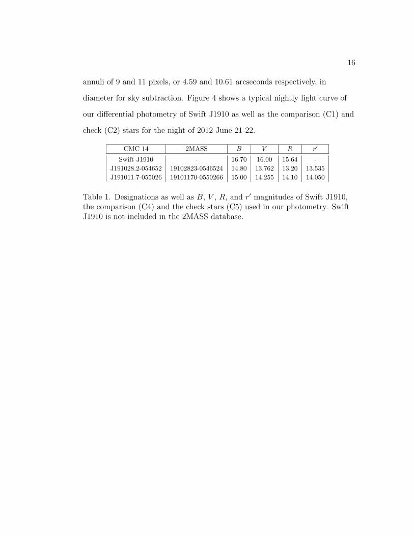
Table 1. Designations as well as B, V , R, and r′ magnitudes of SwiftJ1910, the comparison (C4) and the check stars (C5) used in ourphotometry. Swift J1910 is not included in the 2MASS database. 16

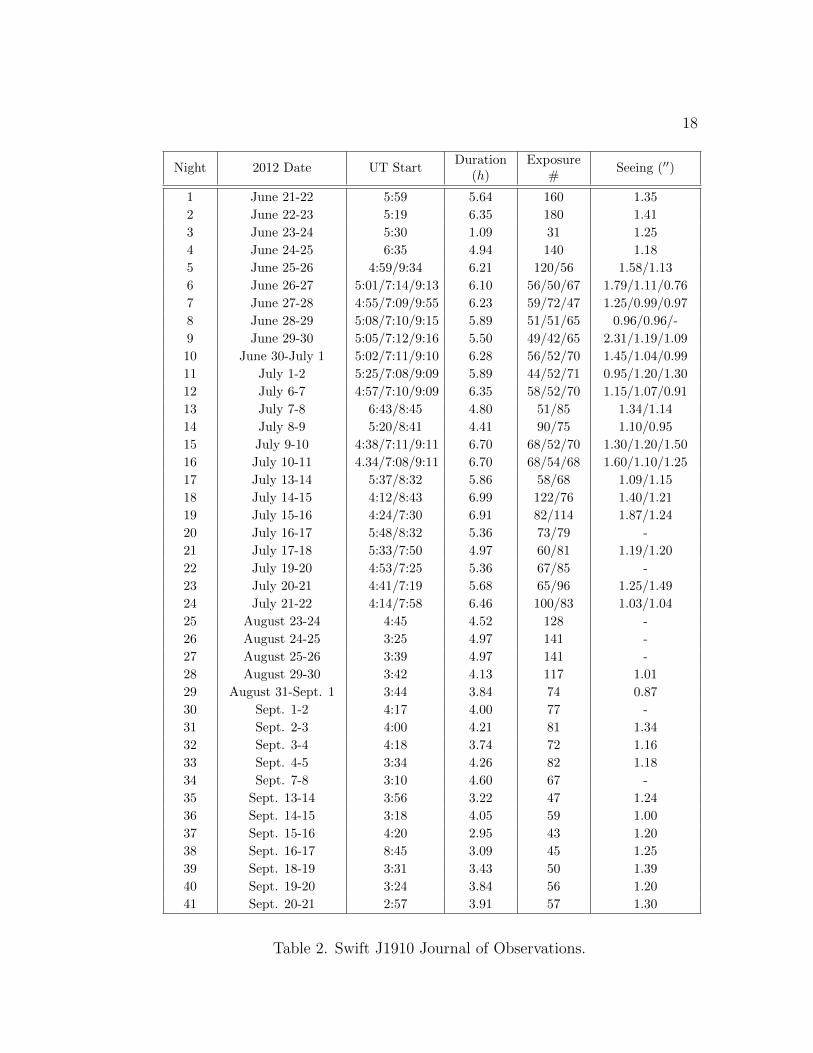
Table 2. Swift J1910 Journal of Observations. . . . . . . . . . . . . . 18

Table 3. Prominent frequencies and errors for all five observing sec-tions. All frequency values are in units of cycles/day. . . . . . . . 44

LIST OF FIGURES

Page

Figure 1. The two types of X-ray binaries: HMXBs and LMXBs. Thetwo insets show the X-ray emission from the respective compactobjects. The Sun is included to scale for prospective. From vanden Heuvel & Taam (1984). . . . . . . . . . . . . . . . . . . . . . 2

Figure 2. Multiwavelength light curve of the prototype SXT A0620-00 during its 1975 outburst showing the amplitudes of the sec-ondary maxima at ∼50 days and ∼170 days. From Kuulkers (1998). 8

Figure 3. Finding chart for Swift J1910 showing the comparison (C4)and check (C5) stars, provided by the British Astronomical Asso-ciation Variable Star Section (Pickard 2012). The field of view is15 arcminutes square. . . . . . . . . . . . . . . . . . . . . . . . . . 17

Figure 4. Differential light curve of Swift J1910 for 2012 June 21-22. 19

Figure 5. Differential light curve of Swift J1910 for all 41 nights. . . 21

Figure 6. The two primary observing seasons and their respectivelight curves (top), Lomb-Scargle periodograms (middle) and spec-tral window functions (bottom). LEFT: June 21-22 until July21-22; RIGHT: August 23-24 until September 20-21. There areno true periodicities in either observing season, only those due toaliasing. . . . . . . . . . . . . . . . . . . . . . . . . . . . . . . . . 23

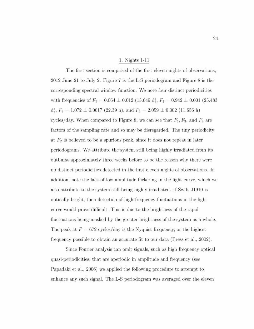
Figure 7. The L-S periodogram for the nights of 2012 June 21 to 2012July 2. . . . . . . . . . . . . . . . . . . . . . . . . . . . . . . . . . 26

Figure 8. The spectral window function for Figure 7. . . . . . . . . . 26

Figure 9. The full L-S periodogram for nights 1-11 of observations.Note the absence of any obvious periodicity. The peak at ∼670cycles/day is from the Nyquist frequency. . . . . . . . . . . . . . . 27

Figure 10. The average power spectrum for nights 1-11 of observations. 27

Figure 11. The L-S periodogram for nights 12-16 of observations. . . . 29

Figure 12. The spectral window function for nights 12-16 of observations. 29

viii

Figure 13. Phase-folded light curve over the proposed orbital periodof 8.117 h. . . . . . . . . . . . . . . . . . . . . . . . . . . . . . . . 30

Figure 14. The full L-S periodogram for nights 12-16 out to the Nyquistfrequency. . . . . . . . . . . . . . . . . . . . . . . . . . . . . . . . 31

Figure 15. The average power spectrum of the light curve from nights12-16. A 4.19 min quasi-periodicity candidate is shown at log(F )= 2.536. . . . . . . . . . . . . . . . . . . . . . . . . . . . . . . . . 31



Figure 18. Phase-folded light curve over the prominent signal in Figure16 of F1 = 3.039 cycles/day (7.897 h). . . . . . . . . . . . . . . . 34

Figure 19. The full L-S periodogram for nights 17-21 of observationsout to the Nyquist frequency. Note the lack of any strong high-frequency signals. . . . . . . . . . . . . . . . . . . . . . . . . . . . 34



Figure 22. Phase-folded light curve over the most prominent 6.8941cycles/day (3.4812 h) signal revealing sinusoidal behavior. . . . . 38

Figure 23. The full L-S periodogram for nights 35-38 including theNyquist frequency at ∼340 cycles/day. Note the general lack ofperiodicities throughout the range of frequencies. . . . . . . . . . 38

Figure 24. The prewhitened L-S periodogram for nights 35-38. Severalperiodicities are revealed in the residuals that resemble those foundin the periodogram for nights 39-41 as seen in Figure 25. . . . . . 39



Figure 27. The full L-S periodogram of nights 39-41 including theNyquist frequency of ∼350 cycles/day. There is strong flickeringbehavior as well as several quasi-periodicity candidates. . . . . . . 43

ix

Figure 28. The average power spectrum for nights 39-41 of observa-tions showing a great deal of high-frequency power with severalquasi-periodicity candidates. . . . . . . . . . . . . . . . . . . . . . 43

Figure 29. Differential photometric light curve through a B band filter. 48

Figure 30. Differential photometric light curve through a V band filter. 49

Figure 31. Differential photometric light curve through an R band filter. 50

Dedicated to Mom and Dad

INTRODUCTION

X-ray binaries are closely-orbiting binary star systems composed of a

compact object and a main sequence companion star. The compact object is

either a neutron star or black hole and are thus the more massive cousins of

cataclysmic variables, whose compact object is a white dwarf. The companion

star is deformed by the stronger gravitational attraction of the compact

object. As soon as the outline of this “teardrop-shaped” deformation of the

companion’s outer layers reaches the critical point for mass to transfer onto

the accretion disk, the companion is said to fill its Roche lobe. The easiest

point for this to occur is located at the pinnacle of the Roche lobe, also known

as the system’s inner Lagrangian point, L1. When the stream of accreted gas

strikes the disk it creates a bright spot on the outer edge that is pulled

tangentially around the plane of the disk. This bright spot also contributes to

the luminosity of the system and can often be seen in light curves of eclipsing

systems. X-ray binaries are divided into two main types based on the optical

companion properties: high mass X-ray binaries (HMXBs) and low mass

X-ray binaries (LMXBs). Figure 1 shows a comparison between HMXBs and

LMXBs. There are several excellent reviews of the properties of X-ray

binaries, namely Paradijs & McClintock (1995), Seward & Charles (2010),

White et al. (1995), Casares (2001), Hellier (2001), and Charles and Coe

(2006).

2

Figure 1. The two types of X-ray binaries: HMXBs and LMXBs. The twoinsets show the X-ray emission from the respective compact objects. The Sunis included to scale for prospective. From van den Heuvel & Taam (1984).

High Mass X-ray Binaries

HMXBs are characterized by young, luminous OB supergiants with

high mass transfer rates (m) via intense stellar wind (typical m ∼ 10−6 M

yr−1) or Roche lobe overflow (see explanation below). Due to their intense

optical emission, the supergiant companion completely overshadows the X-ray

emission from the accretion disk and dominates the overall luminosity of the

system resulting in a Lopt/LX > 1. However, since Swift J1910.2-0546/MAXI

J1910.2-0546 (henceforth referred to as Swift J1910) is an LMXB, the focus of

this thesis will not be on HMXBs.

3

Low Mass X-ray Binaries

LMXBs are characterized by a late-type main sequence companion,

typically a red dwarf, that is constantly being bombarded by a barage of

X-rays from the compact object. The companion absorbs these incident

X-rays and reradiates them in the ultraviolet and optical. They typically have

Lopt/LX < 0.1 with the X-ray flux exhibiting occasional rapid bursts with

exponential decays on timescales of ∼30 seconds. These are believed to be a

result of thermonuclear explosions on the surface of the neutron star (NS

LMXBs). Systems with a black hole as the compact object (BH LMXBs) do

not exhibit X-ray bursts since black holes do not have solid surfaces.

Therefore, it can be said that these rapid X-ray bursts signify the existence of

a neutron star as the compact object. Consequently, this provides an upper

limit on the mass of the system of 3 M, which is the maximum allowable

mass for a neutron star and the minimum mass required to form a black hole

(Casares 2001).

Nomenclature

It would be instructive to explain why these systems are called X-ray

binaries and show that their luminosity has sufficient energies to indeed

radiate in the X-ray spectrum. The luminosity of the system comes from a

combination of the bright spot and the viscosity of the gas as it moves

through the accretion disk. A more massive compact object will generally

result in a high system luminosity since the gas in the accretion disk will be

pulled more quickly onto the compact object. This creates more collisions

4

between the gas particles, the temperature rises due to this increase in friction

and, if occuring across the entire surface area, ultimately results in a higher

disk luminosity. This accretion rate m of gas onto the compact object is

directly proportional to an accretion luminosity:

Lacc =GMm

R(1)

where M and R are the mass and radius of the compact object and G is the

universal gravitational constant. A lower limit of the X-ray flux can be

derived using the lower mass limit for a neutron star of M ' 1.4M, R ' 10

km, and a typical m ' 1016 g s−1, resulting in an accretion luminosity

Lacc ∼ 1036 erg s−1. If the compact object is assumed to absorb and reradiate

precisely all of the incident radiation, known as a blackbody, we can estimate

the temperature of the compact object and thus determine the energy of the

radiation emitted. The accretion luminosity may also be written in terms of

the neutron star’s temperature as:

Lacc = 4πR2σT 4 (2)

where σ is the Stefan-Boltzmann constant. Using a typical neutron star

radius of R ' 10 km results in a temperature of T ' 107 K. A typical photon

at this temperature has an energy kT ' 1 keV, where k is the Boltzmann

constant. Thus, we have a put a lower limit on the energy of emitted

radiation of '1 keV from a typical binary star system containing a neutron

star, which is consistent with radiation in the X-ray spectrum.

5

Soft X-ray Transients

There is a special type of LMXBs that exhibit immense, rapid X-ray

outbursts lasting several days and gradually decay back into quiesence over

several months. These star systems are called soft X-ray transients (SXTs),

sometimes referred to as X-ray novae, and have recurrence times believed to

last from several decades to several centuries. Currently, ∼25% of all SXTs

are confirmed neutron star systems with the remainder being black hole

candidates (Charles & Coe 2006). The reason for this is because in neutron

star systems the outer regions of the disk are irradiated more than in systems

with black holes, due to the fact that there is no definite surface to a black

hole. When accreted gas reaches the black hole it simply disappears without

the creation of radiation. Thus, the outer disk regions of black hole systems

exist in cooler and more un-ionized states, which leads to the buildup of more

gas over longer timescales and eventually the outburst. This is why a

majority of SXTs contain black holes rather than neutron stars.

The leading theory of the origin of outbursts in SXTs is attributed to

the disk (thermal) instability, which has been modeled and theorized for

decades. Photons are tiny quanta of electromagnetic radiation that interact

strongly with charged particles and weakly with neutral atoms. This

phenomenon is illustrated in an accretion disk. Cool, un-ionized hydrogen gas

has a low opacity, or in other words only weakly inhibits the flow of radiation.

Contrarily, hot, ionized hydrogen has a high opacity and does not allow

photons to flow easily. If the temperature of the gas is increased to ∼7,000 K,

the hydrogen atoms will begin to ionize, resulting in a higher opacity.

6

However, more energy is spent in ionizing rather than heating the gas. So in

partially-ionized gas opacity is very sensitive to temperature (see Section 5.3

of Hellier 2001).

Now consider an SXT accretion disk. A small rise in the local

temperature of some region in the disk will result in a higher opacity and

viscosity and slowing down the particle velocities. The gas particles in this

region will fall inwards to a smaller radius from a need to conserve angular

momenum, thus opening up a less dense region of lower opacity and viscosity.

With a small temperature increase, the opacity increases dramatically. Heat is

trapped in the opaque region due to the increased viscous interations and

further increases the temperature. The overall picture is that the energy

trapped in this newly-dense region far outweighs the heat that is trapped in

the same region. There is a snowball effect that continues to permeate the

disk until the system reaches a new quasi-equilibrium. If the amount of gas

entering the disk via Roche lobe overflow from the secondary is insufficient to

maintain the system in this hot, viscous state, then the system goes into

outburst and returns to its original state. As the regions of hot, viscous gas

move inwards, a cooling wave follows. In SXTs, irradiation from the compact

object causes this cooling wave to more inwards on a much longer timescale,

effectively pushing against its inward motion. This is believed to be the

reason why the quiescent intervals among SXTs are so prolonged (Charles &

Coe, 2006).

The companion dominates the optical emission of the system, with

typical quiescent magnitudes of V ∼ 16-23. The light curves typically show

7

erratic, aperiodic flickering behavior with amplitudes of ∼0.2 magnitudes.

Light curves are plots of intensity (W/m2), usually measured in astronomy as

apparent magnitude, as a function of time. The flickering is thought to arise

from the turbulent nature of the accretion disk as clumps of gas randomly

strike the surface of the neutron star. The light curves of SXTs have three

primary characteristics: a sharp rise, an exponential decay, and the presence

of secondary maxima typically occurring ∼50 and ∼170 days after initial

outburst. Figure 2 is the light curve from the first SXT system discovered,

designated A0620-00 in 1975, showing its outburst as well as the secondary

maxima as the system decays back into quiescence.

Origin of the Secondary Maxima

A plethora of theories have been proposed attempting to explain the

origin of these “rebrightenings.” The most popular mechanism to explain this

phenomenon is the disk instability model by Cannizzo, Wheeler, & Ghosh

(1985). Upon initial outburst, the intensity of the X-ray emission increases by

∼106, whereas the optical intensity increases by ∼103. In addition, there is a

stronger emission of hard X-rays (>5 keV) than soft X-rays (∼0.1 keV−5

keV). The hard X-rays decay much faster than their soft counterparts

comprising only 1% of the total flux remaining after ∼60 days (Mineshige

1994). During an outburst, a Compton cloud is formed in the inner region of

the accretion disk near the compact object. This Compton cloud is essentially

a region of very hot, dense, ionized gas that scatters any photons that pass

through. This cloud envelopes the inner accretion disk as well as the spherical

8

Figure 2. Multiwavelength light curve of the prototype SXT A0620-00 duringits 1975 outburst showing the amplitudes of the secondary maxima at ∼50days and ∼170 days. From Kuulkers (1998).

inner coronal region above and below the compact object. During the first

several weeks of the outburst, hard X-rays emitted from the compact object

due to the infall of gas are blocked from escaping to the outer regions of the

disk resulting in a majority of the observed X-ray flux being in the soft

regime. Once the hard X-ray flux sufficiently diminishes, the Compton cloud

evaporates, enabling the hard X-rays to irradiate the outer regions of the disk

and thereby causing secondary heating (Mineshige et al., 1994).

9

There are two primary results of this second heating phase. First, the

companion star is irradiated, causing its surface to heat up, which results in

an increased m. Second, since LMXBs tend to have flared accretion disks, the

upper and lower rim of the flared outer disk is X-ray irradiated. The middle

regions of the outer disk are believed to be blocked from irradiation by the

disk itself. The X-ray irradiation of gas in the outer regions of the disk

increases the temperature of the gas. This increase in temperature comes with

an increase in the viscosity of the gas moving around the disk. A higher

viscosity causes the gas to lose angular momentum and fall in towards the

compact object. If this occurs across the entire disk, then there arises a

collective heating wave that moves inward at essentially the same rate and will

result in a second outburst observable from the optical to X-ray wavelengths.

The entire process is then repeated and is the reason for the rebrightening

seen at ∼170 days in the light curves of SXTs (Seward & Charles 2010).

A Brief History of Observations

As discussed earlier, the nature of soft X-ray transients is that their

outbursts may be separated by decades, which makes observing the same

system through two consecutive outbursts a fairly long and drawn out affair.

This made for exciting times on the night of 2012 May 30-31 when X-rays

first spewed forth and sent astronomers scrambling for observations. Notices

of these observations were posted online using The Astronomer’s Telegram.

The following sections descibe some of the major observations of Swift J1910

so far.

10

ATel #4145

Kennea et al. (2012) reported observations of Swift J1910 on 2012

June 4. No QPOs were detected and they proposed that Swift J1910 was still

in the “thermal” state, which was consistent with no QPO activity

(Remilliard & McClintock 2006).

ATel #4146

On 2012 June 1, Cenko et al. (2012), on behalf of the Palomar

Transient Factory, reported observations of the optical counterpart of Swift

J1910 using an R band filter at a magnitude of R = 15.9.

ATel #4195

Britt et al. (2012) observed Swift J1910 for three nights over 2012

June 1-4 using the 0.9m SMARTS Consortium telescope at the Cerro Tololo

Inter-American Observatory in Chile. They reported optical variability in the

counterpart of r′ = 15.50 ± 0.01 on June 1, r′ = 15.42 ± 0.01 on June 3, and

r′ = 15.40 ± 0.01 on June 4. These magnitude values are the averages of the

data taken on those nights. They also reported dominant flickering activity of

up to 0.1 magnitudes that is evident in all their observations on timescales of

up to an hour. They did not report any significant periodicities in their data.

ATel #4198

Kimura et al. (2012) reported that Swift J1910 was observed to be in a

11

bright soft state and exhibited a soft-to-intermediate X-ray state transition.

On 2012 June 10-12, they observed the 2-4 keV X-ray flux reached a peak of 2

Crab, or ∼4.8 x 10−8 ergs cm−2 s−1. A Crab (or mCrab) is a unit of

astrophotometric measurement used in X-ray astronomy based on the X-ray

flux of the Crab nebula at corresponding energies (the Crab nebula’s intensity

varies at different X-ray energies). They report the 2-4 keV flux decreased

from 2012 June 16-21, the 4-10 keV flux remained approximately constant,

and the 10-20 keV flux tended to increase. These trends indicate a

soft-to-intermediate transition has taken place. In other words, the flux of

lower energetic X-rays is getting smaller while the flux from the more

energetic X-rays is getting more intense.

ATel #4246

Lloyd et al. (2012) report time-series photometry taken with 0.35m to

0.5m class telescopes in Australia, Chile, and the United Kingdom. They

obtained V band observations on 2012 June 27, 28, and 29, and July 1, 6, and

7. They reported the mean V magnitude faded from V = 15.83 to V = 15.98

with various modulations up to 0.3 magnitudes. They performed a

Lomb-Scargle periodogram analysis to search for periodicities and found a

clear set of peaks centered near a frequency of 10.75 cycles/day with a weaker

set near 4.00 cycles/day (these values match our data reasonably well; see

Data Analysis section). They did not report any flickering activity.

ATel #4273

12

Nakahira et al. (2012) reported follow-up observations of Swift J1910

in which they proposed that Swift J1910 was going through the soft-to-hard

state transition. They reported that the 2-4 keV flux decreased slightly from

310 ± 16 mCrab to 270 ± 13 mCrab, while the 4-10 keV flux increased from

33 ± 8 mCrab to 77 ± 8 mCrab and finally to 112 ± 12 mCrab. They

suggested that this behavior between the two energy regimes signified that

Swift J1910 was going through the soft-to-hard state transition, which is

evident in soft X-ray transients.

ATel #4295

King et al. (2012) reported the first radio detections of Swift J1910

from 2012 August 3 with the Jansky Very Large Array. The source was

detected at 2.5 milliJanskys (mJy) at 6 gigaHertz (GHz), where 1 Jansky =

10−26 W m−2 Hz−1. In essence, this corresponds to a rather small detection

level over a very narrow frequency bandwidth. These were the first

documented radio observations of Swift J1910.

ATel #4328

Bodaghee et al. (2012) reported observations of Swift J1910 emitting

in the hard X-rays using INTEGRAL’s hard X-ray imager (ISGRI). From

data taken on the night of 2012 August 20-21, the system was detected in the

18-40 keV range at a high significance level of 13.7σ and in the 40-100 keV

range at a significance level of 9.4σ. ISGRI also detected Swift J1910 up to

energies of ∼200 keV. These detections confirmed that Swift J1910 was indeed

13

in the hard state.

ATel #4347

Casares et al. (2012) reported on R band photometry of Swift J1910 of

over 3.1 hours on the night of 2012 July 21 using the 2.5m Nordic Optical

Telescope. They measured a mean magnitude of R = 16.20. This is in slight

disagreement with our own R band observations shown in Figure 31 that give

a mean magnitude of R ∼ 15.76 during this same night, which, luckily

enough, was our final night of R band observations. For a further discussion

of our calculated B, V , and R magnitudes see the B, V , & R Photometry

section. In addition, they proposed an orbital period of >6.2 hours due to

spectroscopic radial velocity observations of Hα emission from the optical

counterpart. This appears to be the lowest frequency periodicity seen in

Figures 11, 16, 20, and 25, which we propose may resemble either the

precessional period or the orbital period of the system.

OBSERVATIONS

Time-resolved differential CCD photometry was carried out beginning

on the night of 2012 June 21-22 UT and continued until 2012 September

19-20 UT. In this time, we collected 43 nights of data, 41 of which were

included in our analysis. The night of 2012 July 2-3 was unusable because of

the proximity to the Full Moon and the night of 2012 August 26-27 unusable

due to complications in the data reduction. Table 2 is a journal of our

observations.

We used the 0.41m (16 in) f/8 telescope by DFM Engineering at

Fresno State’s station at Sierra Remote Observatories and a Santa Barbara

Instruments Group STL-11000M CCD camera. Frames were exposed for 120

seconds with a dead time to read out the CCD between exposures of 7

seconds, making for a total time resolution of 254 seconds. Due to the target

being a soft X-ray transient, its brightness was gradually diminishing and, in

the later months, required a longer exposure time. In order to ensure we

continued to collect enough light, we increased the exposure time from 120

seconds to 180 seconds beginning on 2012 August 31-September 1 and

ulitmately to 240 seconds on 2012 September 13-14, which continued through

the rest of our observations. The dead time for each exposure remained at 7

seconds, making for a new time resolution of 494 seconds.

All exposures were taken through a Clear luminance filter by

Astrodon. The Clear filter allows for the maximum amount of light to enter

the CCD camera, which is optimal since our target is very faint at

approximately 16th-17th magnitude. Weather was clear and apparently

15

photometric on most nights. However, there were a few nights that appeared

to be marginally obscured by clouds or haze.

All data were processed with AIP4WIN 2.1.8 software (Berry &

Burnell, 2005). All exposures were dark-subtracted, but not divided by a flat

field. The CCD temperature was set to -5C for all exposures. Fifteen dark

frames were collected every night. These dark frames were median-combined

to form a master dark frame, which was then subtracted from each of the

target frames.

To measure the photometry we used comparison and check stars that

are preferred by the British Astronomical Association Variable Star Section

(BAAVSS), who first observed the target on 2012 June 14 (Pickard 2012).

Figure 3 is the finding chart provided by the BAAVSS and the comparison

and check stars that we used are labeled as C4 and C5, respectively. Note

that the designations by the BAAVSS of the comparison and check stars as

C4 and C5, respectively, are different from the designations that we use for

the comparison and check stars as C1 and C2, respectively, in our plots. The

BAAVSS used the Carlsberg Meridian Catalogue 141 (CMC 14) names, so in

order to determine the magnitudes in the other filters the Two Micron All Sky

Survey (2MASS) was consulted. Table 1 lists the CMC 14 and 2MASS

designations of V , C4, and C5 as well as their magnitudes in each filter.

Our telescope and camera have an image scale of 0.51

arcseconds/pixel. All of our observations were done using 3x3 binning,

making for an image scale of 1.53 arcseconds/pixel. All photometry used an

aperture of 6 pixels, or 3.06 arcseconds, in diameter, and used inner and outer

16

annuli of 9 and 11 pixels, or 4.59 and 10.61 arcseconds respectively, in

diameter for sky subtraction. Figure 4 shows a typical nightly light curve of

our differential photometry of Swift J1910 as well as the comparison (C1) and

check (C2) stars for the night of 2012 June 21-22.

CMC 14 2MASS B V R r′

Swift J1910 - 16.70 16.00 15.64 -

J191028.2-054652 19102823-0546524 14.80 13.762 13.20 13.535

J191011.7-055026 19101170-0550266 15.00 14.255 14.10 14.050

Table 1. Designations as well as B, V , R, and r′ magnitudes of Swift J1910,the comparison (C4) and the check stars (C5) used in our photometry. SwiftJ1910 is not included in the 2MASS database.

17

Figure 3. Finding chart for Swift J1910 showing the comparison (C4) andcheck (C5) stars, provided by the British Astronomical Association VariableStar Section (Pickard 2012). The field of view is 15 arcminutes square.

18

Night 2012 Date UT StartDuration

(h)Exposure

#Seeing (′′)

1 June 21-22 5:59 5.64 160 1.35

2 June 22-23 5:19 6.35 180 1.41

3 June 23-24 5:30 1.09 31 1.25

4 June 24-25 6:35 4.94 140 1.18

5 June 25-26 4:59/9:34 6.21 120/56 1.58/1.13

6 June 26-27 5:01/7:14/9:13 6.10 56/50/67 1.79/1.11/0.76

7 June 27-28 4:55/7:09/9:55 6.23 59/72/47 1.25/0.99/0.97

8 June 28-29 5:08/7:10/9:15 5.89 51/51/65 0.96/0.96/-

9 June 29-30 5:05/7:12/9:16 5.50 49/42/65 2.31/1.19/1.09

10 June 30-July 1 5:02/7:11/9:10 6.28 56/52/70 1.45/1.04/0.99

11 July 1-2 5:25/7:08/9:09 5.89 44/52/71 0.95/1.20/1.30

12 July 6-7 4:57/7:10/9:09 6.35 58/52/70 1.15/1.07/0.91

13 July 7-8 6:43/8:45 4.80 51/85 1.34/1.14

14 July 8-9 5:20/8:41 4.41 90/75 1.10/0.95

15 July 9-10 4:38/7:11/9:11 6.70 68/52/70 1.30/1.20/1.50

16 July 10-11 4.34/7:08/9:11 6.70 68/54/68 1.60/1.10/1.25

17 July 13-14 5:37/8:32 5.86 58/68 1.09/1.15

18 July 14-15 4:12/8:43 6.99 122/76 1.40/1.21

19 July 15-16 4:24/7:30 6.91 82/114 1.87/1.24

20 July 16-17 5:48/8:32 5.36 73/79 -

21 July 17-18 5:33/7:50 4.97 60/81 1.19/1.20

22 July 19-20 4:53/7:25 5.36 67/85 -

23 July 20-21 4:41/7:19 5.68 65/96 1.25/1.49

24 July 21-22 4:14/7:58 6.46 100/83 1.03/1.04

25 August 23-24 4:45 4.52 128 -

26 August 24-25 3:25 4.97 141 -

27 August 25-26 3:39 4.97 141 -

28 August 29-30 3:42 4.13 117 1.01

29 August 31-Sept. 1 3:44 3.84 74 0.87

30 Sept. 1-2 4:17 4.00 77 -

31 Sept. 2-3 4:00 4.21 81 1.34

32 Sept. 3-4 4:18 3.74 72 1.16

33 Sept. 4-5 3:34 4.26 82 1.18

34 Sept. 7-8 3:10 4.60 67 -

35 Sept. 13-14 3:56 3.22 47 1.24

36 Sept. 14-15 3:18 4.05 59 1.00

37 Sept. 15-16 4:20 2.95 43 1.20

38 Sept. 16-17 8:45 3.09 45 1.25

39 Sept. 18-19 3:31 3.43 50 1.39

40 Sept. 19-20 3:24 3.84 56 1.20

41 Sept. 20-21 2:57 3.91 57 1.30

Table 2. Swift J1910 Journal of Observations.

19

Figure 4. Differential light curve of Swift J1910 for 2012 June 21-22.

DATA ANALYSIS

Figure 5 shows the differential light curve of all 41 nights used in our

analysis. Swift J1910 was discovered to have gone into outburst on the night

of 2012 May 30-31 simultaneously by the hard X-ray transient monitor aboard

NASA’s Swift Burst Alert Telescope on NASA’s Swift Gamma Ray

Observatory and Monitor of All-sky X-ray Image (MAXI) aboard the

International Space Station. Since our observations began on 2012 June

21-22, we note a gradual downward trend in the optical V − C1 light curve as

well as a definite rise, or rebrightening, ∼190 days after initial outburst. This

secondary maxima, at ∼50 and ∼170 days, are characteristic features of soft

X-ray transients. We suspect that the first rebrightening at ∼50 days

occurred during the hiatus in our observations and that the bump we see in

our light curve beginning around 2456170 Julian days (JD), or August 30, is

actually the second rebrightening.

We excluded several nights because of occasional fluctuations such as

passing satellites or cosmic rays incident on the CCD detector that were

outliers in the light curve and would have otherwise biased our data. No

obvious periodicities could be determined from the periodogram analysis of all

41 nights, which was dominated by strong aliasing due to so many gaps in our

observations (see Box 9.1 of Hellier, 2001). To try and overcome this, we

divided the data set into two observing sessions in hopes of determining more

accurate periodicities. Figure 6 shows how the two observing seasons compare

with one another. We list the V − C1 light curves for both observing seasons

21

Figure 5. Differential light curve of Swift J1910 for all 41 nights.

with their respective Lomb-Scargle (L-S) periodograms (Lomb 1976; Scargle

1982; Press et al., 1992) that we calculated with the PERANSO (PEriod

ANalysis SOftware) software package (Vanmunster, 2009), and spectral

window functions (SWFs). Light curves are plots of intensity, measured as

apparent magnitude and typically having units of W/m2 as a function of time.

The V − C1 curve shows how much the intensity of the variable (Swift J1910

in this case) changes when compared to a companion star. The C2− C1

curve should be as flat as possible in order to prove that the intensity of the

companion star does not change as well. Thus, by direct comparison of both

curves, any variability of Swift J1910 can be seen. A L-S periodogram is used

to search for periodicities in the light curves. The spectral window function

22

shows how the sampling rate affects our periodogram due to convolution with

the diurnal cycle. For instance, if observations were made every night for 6

hours for one week, the SWF would show a strongest peak at 1 cycle/day and

less prominent peaks at 2 cycles/day, 3 cycles/day, etc. For a more detailed

discussion of the convolution theorem and the diurnal cycle see Press et al.

(1992). There are no definite periodicities that can be seen in either

periodogram. The periodogram for Weeks 1-5 has strong peaks at 0.025,

1.019, and 2.021 cycles/day and the periodogram for Weeks 10-15 has strong

peaks at 0.027, 0.970, and 1.976 cycles/day. Since these frequencies are all

separated by ∼1 cycle/day, they should not be trusted as true variability due

to the strong probability of being biased from observing on consecutive nights.

Additionally, all peaks in the SWFs align with all peaks in the

periodograms, which tells us that those periodicities arise from our sampling

rate. If there were peaks in the periodogram that did not have a

corresponding peak in the SWF at the same frequency, then this would

indicate variability due to optical modulation in the accretion disk. Each

strong peak in the periodogram is accompanied by smaller peaks on each side.

These smaller peaks are aliases since they repeat with every strong peak in

the periodogram and thus cannot be construed as true variability.

Since no periodic variability could be determined from the light curves

of the two observing seasons individually, we further divided the data into five

sections. These sections were chosen based on the number of consecutive

nights of observations, since it is preferred to have as many consecutive nights

as possible for the periodogram analysis.

23

Figure 6. The two primary observing seasons and their respective light curves(top), Lomb-Scargle periodograms (middle) and spectral window functions(bottom). LEFT: June 21-22 until July 21-22; RIGHT: August 23-24 untilSeptember 20-21. There are no true periodicities in either observing season,only those due to aliasing.

24

1. Nights 1-11

The first section is comprised of the first eleven nights of observations,

2012 June 21 to July 2. Figure 7 is the L-S periodogram and Figure 8 is the

corresponding spectral window function. We note four distinct periodicities

with frequencies of F1 = 0.064 ± 0.012 (15.649 d), F2 = 0.942 ± 0.001 (25.483

d), F3 = 1.072 ± 0.0017 (22.39 h), and F4 = 2.059 ± 0.002 (11.656 h)

cycles/day. When compared to Figure 8, we can see that F1, F3, and F4 are

factors of the sampling rate and so may be disregarded. The tiny periodicity

at F2 is believed to be a spurious peak, since it does not repeat in later

periodograms. We attribute the system still being highly irradiated from its

outburst approximately three weeks before to be the reason why there were

no distinct periodicities detected in the first eleven nights of observations. In

addition, note the lack of low-amplitude flickering in the light curve, which we

also attribute to the system still being highly irradiated. If Swift J1910 is

optically bright, then detection of high-frequency fluctuations in the light

curve would prove difficult. This is due to the brightness of the rapid

fluctuations being masked by the greater brightness of the system as a whole.

The peak at F = 672 cycles/day is the Nyquist frequency, or the highest

frequency possible to obtain an accurate fit to our data (Press et al., 2002).

Since Fourier analysis can omit signals, such as high frequency optical

quasi-periodicities, that are aperiodic in amplitude and frequency (see

Papadaki et al., 2006) we applied the following procedure to attempt to

enhance any such signal. The L-S periodogram was averaged over the eleven

25

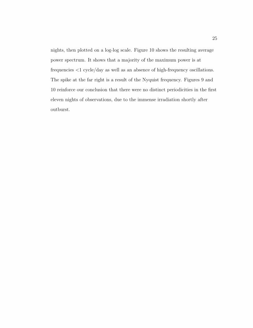
nights, then plotted on a log-log scale. Figure 10 shows the resulting average

power spectrum. It shows that a majority of the maximum power is at

frequencies <1 cycle/day as well as an absence of high-frequency oscillations.

The spike at the far right is a result of the Nyquist frequency. Figures 9 and

10 reinforce our conclusion that there were no distinct periodicities in the first

eleven nights of observations, due to the immense irradiation shortly after

outburst.

26

Figure 7. The L-S periodogram for the nights of 2012 June 21 to 2012 July 2.

Figure 8. The spectral window function for Figure 7.

27

Figure 9. The full L-S periodogram for nights 1-11 of observations. Note theabsence of any obvious periodicity. The peak at ∼670 cycles/day is from theNyquist frequency.

Figure 10. The average power spectrum for nights 1-11 of observations.

28

2. Nights 12-16

The next group of consecutive observations was nights 12-16, or 2012

July 6-11. Figure 11 is the L-S periodogram and Figure 12 is the

corresponding SWF. The periodogram shows prominent frequencies of F1 =

2.9565 ± 0.0999 cycles/day, corresponding to a period of 8.117 ± 0.011 h and

F2 = 10.7472 ± 0.0038 cycles/day, corresponding to a period of 2.2331 h.

Notice that the peaks in the SWF do not correspond to the prominent peaks

in Figure 11, which means that frequencies F1 and F2 are real variabilities in

Swift J1910. Figure 13 shows the light curve folded over the most prominent

frequency of 2.9565 cycle/day (8.117 h).

Figure 14 shows higher levels of aperiodic flickering than in the L-S

periodogram for nights 1-11 shown in Figure 9. We believe this to be from the

disk becoming less irradiated over time and allowing the optical light to be

more easily observed. The Nyquist frequency at F = 670 cycles/day is also

included for completeness. There is a quasi-periodicity candidate at a

frequency of 343.534 cycles/day, or ∼4.19 min, which is roughly 40% stronger

than the surrounding mean noise level. Figure 15 shows the average power

spectrum calculated as described earlier. There is a large amount of

low-frequency variability present in the data for these nights. A distinct spike

at log(F cycles/day) = 2.536 matches the signal found in the L-S

periodogram in Figure 14. Since this signal remains after calculation of the

average power spectrum, I conclude this 4.19 min quasi-periodicity to be real.

29

Figure 11. The L-S periodogram for nights 12-16 of observations.

Figure 12. The spectral window function for nights 12-16 of observations.

30

Figure 13. Phase-folded light curve over the proposed orbital period of8.117 h.

31

Figure 14. The full L-S periodogram for nights 12-16 out to the Nyquistfrequency.

Figure 15. The average power spectrum of the light curve from nights 12-16.A 4.19 min quasi-periodicity candidate is shown at log(F ) = 2.536.

32

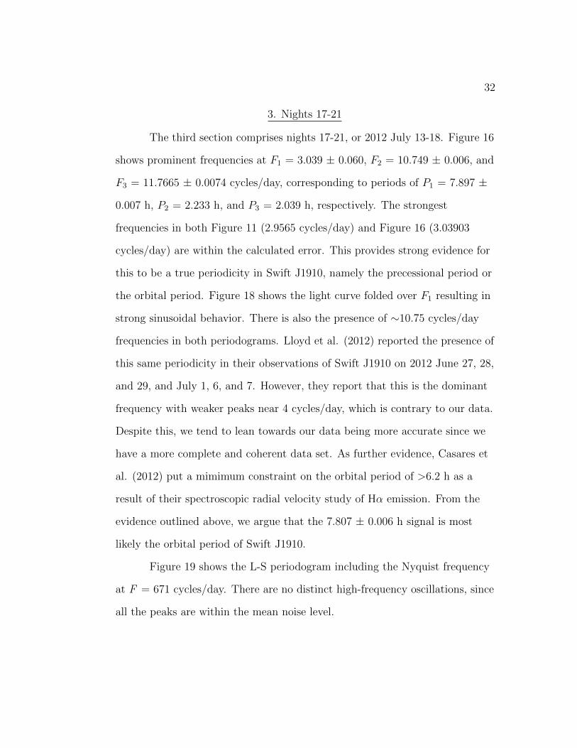
3. Nights 17-21

The third section comprises nights 17-21, or 2012 July 13-18. Figure 16

shows prominent frequencies at F1 = 3.039 ± 0.060, F2 = 10.749 ± 0.006, and

F3 = 11.7665 ± 0.0074 cycles/day, corresponding to periods of P1 = 7.897 ±

0.007 h, P2 = 2.233 h, and P3 = 2.039 h, respectively. The strongest

frequencies in both Figure 11 (2.9565 cycles/day) and Figure 16 (3.03903

cycles/day) are within the calculated error. This provides strong evidence for

this to be a true periodicity in Swift J1910, namely the precessional period or

the orbital period. Figure 18 shows the light curve folded over F1 resulting in

strong sinusoidal behavior. There is also the presence of ∼10.75 cycles/day

frequencies in both periodograms. Lloyd et al. (2012) reported the presence of

this same periodicity in their observations of Swift J1910 on 2012 June 27, 28,

and 29, and July 1, 6, and 7. However, they report that this is the dominant

frequency with weaker peaks near 4 cycles/day, which is contrary to our data.

Despite this, we tend to lean towards our data being more accurate since we

have a more complete and coherent data set. As further evidence, Casares et

al. (2012) put a mimimum constraint on the orbital period of >6.2 h as a

result of their spectroscopic radial velocity study of Hα emission. From the

evidence outlined above, we argue that the 7.807 ± 0.006 h signal is most

likely the orbital period of Swift J1910.

Figure 19 shows the L-S periodogram including the Nyquist frequency

at F = 671 cycles/day. There are no distinct high-frequency oscillations, since

all the peaks are within the mean noise level.

33



34

Figure 18. Phase-folded light curve over the prominent signal in Figure 16 ofF1 = 3.039 cycles/day (7.897 h).

Figure 19. The full L-S periodogram for nights 17-21 of observations out tothe Nyquist frequency. Note the lack of any strong high-frequency signals.

35

4. Nights 35-38

The fourth section spans nights 35-38, or 2012 September 13-17. The

only prominent periodicity is F1 = 6.8941 ± 0.0998 cycles/day, corresponding

to a period of 3.4812 h, as well as the standard 1 cycle/day aliases. The fact

that this is the only signal is rather perplexing because there is no comparable

signal arising within the error in the periodograms for the other sections

(Figures 7, 11, 16, and 25). This value is about half of the lower limit of 6.2

cycles/day by Casares et al. (2012) obtained by spectroscopic radial velocity

studies of the Hα emission from the companion. It is a definite signal since it

does not coincide with identical frequencies in the SWF in Figure 21.

Unfortunately, we do not have a good reason as to why the proposed orbital

period of 7.897 h is absent in this periodogram. It may be possible that since

the rebrightening occurred a mere 14 days before, there was still a residual

luminosity that masked any shorter variability though further study is

required to be certain. Figure 22 is the light curve folded over the prominent

6.8941 cycles/day signal and sinusoidal behavior is evident. Figure 23 is the

full L-S periodogram including the Nyquist frequency of 340 cycles/day.

There is no distinct quasi-periodic behavior evident in this periodogram.

In order to search for any periodicities that were not evident in the

original periodogram analysis in Figure 20, we subtracted the prominent

signal of F1 = 6.8941 cycles/day from the observations and began a new

periodogram analysis on the residual data. If a new signal appears in the

residual periodogram, then the system may contain multiple periodicities such

as the disk’s precessional period, orbital period, and superhump period. This

36

method is called prewhitening and is very useful for finding “hidden” signals

in the data. Figure 24 shows the prewhitened periodogram with the 6.8941

cycles/day signal cut out and very closely resembles the regular periodogram

for nights 39-41 seen in Figure 25. However, upon closer comparison of the

two periodograms, we notice that the four prominent signals of the

prewhitened periodogram in Figure 24 all reside ≤30 cycles/day, whereas the

four prominent signals of the regular periodogram in Figure 25 are less spread

out and reside ≤25 cycles/day. One possibility for this is that if the data from

nights 35-38 were still experiencing lingering effects from the recent

rebrightening, which would result in a higher disk viscosity and luminosity,

the movement of gas throughout the disk would have been hindered. Thus the

gas would move slower and result in lower-frequency signals. So as the disk

became less viscous and more transparent to light, the frequency of the

observed periodicities would decrease.

37



38

Figure 22. Phase-folded light curve over the most prominent 6.8941cycles/day (3.4812 h) signal revealing sinusoidal behavior.

Figure 23. The full L-S periodogram for nights 35-38 including the Nyquistfrequency at ∼340 cycles/day. Note the general lack of periodicitiesthroughout the range of frequencies.

39

Figure 24. The prewhitened L-S periodogram for nights 35-38. Severalperiodicities are revealed in the residuals that resemble those found in theperiodogram for nights 39-41 as seen in Figure 25.

40

5. Nights 39-41

The fifth and final section of consecutive observations are nights 39-41,

or 2012 September 18-21. Figure 25 is the L-S periodogram and shows four

distinct signals at F1 = 4.0605 ± 0.0499 cycles/day (5.9106 h), F2 = 11.0188

± 0.0014 cycles/day (2.1781 h), F3 = 18.1766 ± 0.0048 cycles/day (1.3204 h),

and F4 = 25.0101 ± 0.0024 cycles/day (57.57 min). We can see that none of

these signals coincide with the signals in the spectral window function seen in

Figure 26. The signals at ∼4 and ∼11 cycles/day are present in this

periodogram just as they were in the periodogram for night 12-16, nights

17-21 and the prewhitened periodogram for nights 35-38. The persistence of

these signals in the data spanning several months of observations is a very

convincing case for them being true periodicities in Swift J1910.

Figure 27 is the full L-S periodogram including the Nyquist frequency

∼350 cycles/day. There is a quasi-periodicity candidate at 110.087 cycles/day,

corresponding to a duration of 13.08 min. Figure 28 is the average power

spectrum and was calculated using the method described earlier in the text.

We note the prominent low-frequency signal of 5.91 h, the 1.32 h signal due to

the ∼18 cycles/day peaks seen in Figure 27, and the quasi-periodicity

candidate signal of 13.08 min. Since the method used to calculated the

average power spectrum does not cut out short, aperiodic fluctuations, we

believe that this signal of a 13.08 min quasi-periodicity to be real because a

distinct spike in the power spectrum is present. Additionally, there is a great

deal of high-frequency power, which is characteristic of increased flickering

behavior that is evident in the periodogram. The signal at the far right of

41

Figure 28 is the Nyquist frequency.

42



43

Figure 27. The full L-S periodogram of nights 39-41 including the Nyquistfrequency of ∼350 cycles/day. There is strong flickering behavior as well asseveral quasi-periodicity candidates.

Figure 28. The average power spectrum for nights 39-41 of observationsshowing a great deal of high-frequency power with several quasi-periodicitycandidates.

44

Nights 1-11 Nights 12-16 Nights 17-21 Nights 35-38 Nights 39-41

Frequency Error Frequency Error Frequency Error Frequency Error Frequency Error

0.064 0.012 2.9565 0.0999 3.039 0.060 6.8941 0.0998 4.0605 0.0499

0.942 0.001 10.7472 0.0038 10.749 0.007 - - 11.0188 0.0014

1.0715 0.0017 - - 11.7665 0.0074 - - 18.1766 0.0048

2.059 0.002 - - - - - - 25.0101 0.0024

Table 3. Prominent frequencies and errors for all five observing sections. Allfrequency values are in units of cycles/day.

Superhumps

Superhumps are a phenomenon in many closely-orbiting binary star

systems. As discussed in Chapter 6 of Hellier (2001), nodal, or negative,

superhumps refer to waves in the disk that are perpendicular to the disk plane

and apsidal, or positive, superhumps refer to the disk becoming elongated

producing waves that precess in the plane of the disk. The precessional period

Pprec of the disk and the orbital period Porb of the system may align with one

another and produce a “beating” pattern that can be seen in the light curve.

If we interpret the 4.0605 cycles/day (5.91 h) signal to be the precessional

period Pprec and the 10.7485 (2.23 h) cycles/day signal to be the orbital

period Porb, we predict an apsidal superhump period Psh of 3.59 h (see page

77 of Hellier, 2001) using the equation

1

Psh

=1

Porb

− 1

Pprec

(3)

This matches the value for the prominent period in the periodogram analysis

of nights 35-38 seen in Figure 20. As discussed in Section 6.3 of Hellier (2001),

45

the superhump period reaches a maximum amplitude around the time of the

peak of an outburst in a cataclysmic variable. We believe this may be applied

to Swift J1910 as well and that since nights 35-38 were close to the

rebrightening phase, the superhump period could very well dominate any

other periodicity during this time. This is the significance of the prewhitened

periodogram of Figure 24. If the proposed Porb is cut out of the periodogram,

then we observe the normal periodicities that are evident for multiple sections

of observations.

However, the interpretation of the superhump period as 6.8941

cycles/day (3.4812 h) is refuted by the discussion of superhumps in Patterson

et al. (2005). We found signals at 4.0605, 11.0188, 18.1766, and 25.0101

cycles/day in the analysis of nights 39-41. These coincide well to the “beat”

progression described by Ω, Porb, 2Porb - Ω, and 3Porb - Ω, where Ω = 1/Pprec.

Superhumps are usually several percent longer (positive) or shorter (negative)

than Porb. Using our values for Psh and Porb, we find a period excess ε =

0.559, where

ε =Psh − Porb

Porb

(4)

Unfortunately, there are some problems with our calculations. First, in

a typical binary star system, a larger value of Psh - Porb implies that the

compact object is much more massive than the secondary (known as the mass

ratio q). We note that our values of 74.89 min for this period difference and

0.559 for the period excess are extremely large. Haswell et al. (2001) used

typical q values of ∼0.102 for SXTs. Second, Patterson et al. (2005) gives an

46

empirical formula for relating the period excess to the mass ratio q as

ε = 0.18q + 0.29q2. Solving this equation for q results in a mass ratio of q =

1.11. Since superhumps can only occur in binary star systems with q ≤ 0.33

as is descibed in Whitehurst & King (1991), our mass ratio of q = 1.11 is

physically impossible. These inconsistencies point to either we have predicted

incorrect period values or there are no superhumps in the system after all.

The latter conclusion is somewhat curious because the observed periodicities

agreed with those obtained through Equation 3. Nonetheless, the egregious

values for the period excess and mass ratio lead us to conclude that

superhumps were not detected in Swift J1910.

It is entirely possible that the low-frequency ∼8 h signal in the L-S

periodograms of Figures 11, 16, 22, and 25 is actually the orbital period of

Swift J1910 and not the precessional period. This would be supported by

observations by Casares et al. (2012). In fact, we believe this to be more

likely since the period excess is so large otherwise.

B, V , and R band Photometry

We took differential photometry of Swift J1910 through

Johnson-Morgan Blue (B) and Visual (V ) filters, as well as a Kron-Cousins

Red (R) filter. These were taken over the first five weeks of observations in

addition to our regular observations. The light curves are shown in Figure 29

(B band), Figure 30 (V band), and Figure 31 (R band). We note gradual

downward trends in all three light curves as expected. More specifically, the

luminosity of the system in the B band in Figure 29 is about the same as that

47

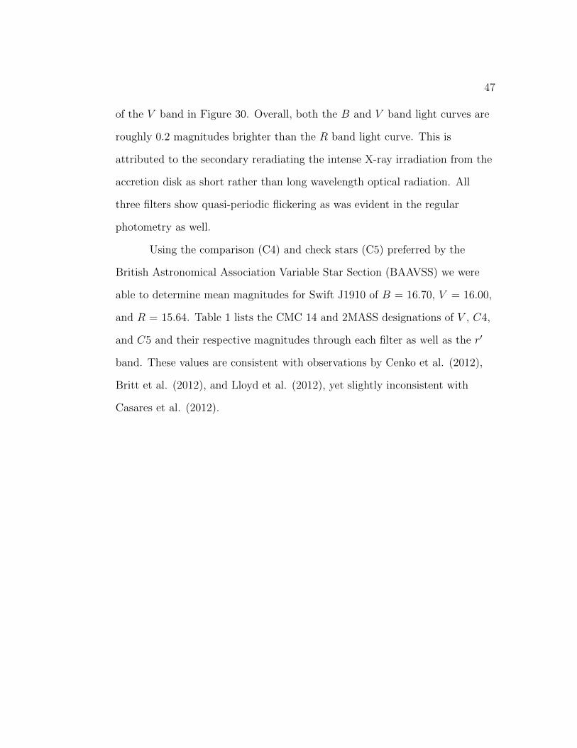
of the V band in Figure 30. Overall, both the B and V band light curves are

roughly 0.2 magnitudes brighter than the R band light curve. This is

attributed to the secondary reradiating the intense X-ray irradiation from the

accretion disk as short rather than long wavelength optical radiation. All

three filters show quasi-periodic flickering as was evident in the regular

photometry as well.

Using the comparison (C4) and check stars (C5) preferred by the

British Astronomical Association Variable Star Section (BAAVSS) we were

able to determine mean magnitudes for Swift J1910 of B = 16.70, V = 16.00,

and R = 15.64. Table 1 lists the CMC 14 and 2MASS designations of V , C4,

and C5 and their respective magnitudes through each filter as well as the r′

band. These values are consistent with observations by Cenko et al. (2012),

Britt et al. (2012), and Lloyd et al. (2012), yet slightly inconsistent with

Casares et al. (2012).

48

Figure 29. Differential photometric light curve through a B band filter.

49

Figure 30. Differential photometric light curve through a V band filter.

50

Figure 31. Differential photometric light curve through an R band filter.

CONCLUSIONS

Forty-one nights of differential photometry of the SXT/black hole

candidate Swift J1910 have been presented. We found multiple periodicities in

all five observing sections that spanned from 2012 June 21-22 to 2012

September 20-21. We propose two possible orbital period scenarios:

First, an orbital period of Porb = 2.233 h (10.749 cycles/day) was

proposed since it was the only periodicity found to repeat itself, within a

standard deviation, in two of the five observing sections. This value for the

orbital period is supported by spectroscopic radial velocity studies of the

companion’s Hα emission by Casares et al. (2012).

A search for superhumps was performed but no indication of which

was found. The period difference of Psh − Porb = 74.89 min and the period

excess of ε = 0.559 were both greatly above the normal values. We obtained a

mass ratio q = 1.11, which is physically impossible for binary star systems

(Whitehurst & King 1991).

Swift J1910 is rife with aperiodic behavior, including a large amount of

flickering. This is characteristic of LMXBs, though more evident primarily

during the less luminous times of the decline (i.e. not during the

rebrightening phase). Optical quasi-periodicitiess were believed to have been

detected of 4.19 min during nights 12-16 and 13.08 min during nights 39-41.

By comparing Figure 15 with Figure 28, we see that there is a definite

increase in high-frequency power. This is believed to be because, after initial

outburst, the temperature of the system cools sufficiently so that the disk

becomes optically transparent, which makes it easier to observe the tiny

52

fluctuations of material infalling onto the compact object.

Observations through B, V , and R filters were performed. In all three

filters, the aperiodic flickering behavior on the timescale of several days was

still evident as well as a gradual decrease in magnitude throughout all nights

of observations. Mean magnitude values of B = 16.70, V = 16.00, and R =

15.64 were obtained. These values make sense with the companion star

reradiating the incident X-rays, resulting in an optical flux for the system

containing more short wavelength light than long wavelength light. In general,

these values agree with previous observations of Cenko et al. (2012), Britt et

al. (2012), and Lloyd et al. (2012), however marginally disagree with those of

Casares et al. (2012). Further observations in all wavelengths are encouraged

and required to support or deny our conclusions.

REFERENCES

Bodaghee et al., (2012) ATel 4328.

Berry, R., Burnell, J., 2005. The Handbook of Astronomical ImageProcessing, Willmann-Bell, Richmond, VA.

Britt et al. (2012) ATel 4195.

Casares et al. (2012) ATel 4347.

Casares, J., X-ray Binaries and Black Hole Candidates: A Review of OpticalProperties. In: Binary Stars, Selected Topics on Observations and PhysicalProcesses, edited by F. C. Lazaro & M. J. Arevalo (2001) 563, 277.

Cannizzo, J. K., Wheeler, J. C., Ghosh, P., Cataclysmic Variables andLow-Mass X-ray Binaries, edited by D. Q. Lamb and J. Patterson (1985), p.307.

Cenko, S. B., Ofek, E. O. (2012) ATel 4146.

Charles, P. A., Coe, M. J., 2006. Compact Stellar X-ray Sources, CambridgeUniv. Press, Cambridge.

Cutri, R. M., Strutskie, M. F., van Dyk, S., Beichman, C. A., Carpenter, J.M., Chester, T., Cambresy, L., Evans, T., Fowler, J., Gizis, J., Howard, E.,Huchara, J., Jarrett, T., Kopan, E. L., Kirkpatrick, J. D., Light, R. M.,Marsh, K. A., McCallon, H., Schneider, S., Stiening, R., Sykes, M., Weinber,M., Weinber, M., Wheaton, W.A., Wheelock, S., Zacarias, N., 2003 The IRSA2MASS All-Sky Point Source Catalog, NASA/IPAC Infrared Science Archive.http://irsa.ipac.caltech.edy/applications/Gator/.

Haswell, C. A., King, A. R., Murray, J. R., Charles, P. A., 2001. MNRAS 321,475.

Hellier, C., 2001. Cataclysmic Variables: How and Why They Vary, PraxisPublishing Ltd., Cornwall, U.K.

54

Kennea et al. (2012) ATel 4145.

Kimura et al. (2012) ATel 4198.

King et al. (2012) ATel 4295.

Kuulkers, E., 1998. NewAR 42, 1.

Lomb, N. R., 1976. ApSS 39, 447.

Lloyd et al. (2012) ATel 4246.

Mineshige, S., 1994. ApJ 431, 99.

Mineshige, S., Hirano, A., Kitamoto, S., Yamada, T. T., Fukue, J., 1994. ApJ426, 308.

Nakahira et al. (2012) ATel 4273.

Patterson, J. et al., 2005. PASP 117, 1204.

Papadaki, C., Boffin H. M. J., Sterken C., Stanishev V., Cuypers J., BoumisP., Akras S., Alikakos J., 2006. A&A 456, 599.

Pickard, R., 2012, www.britastro.org/vss/.

Press, W. H., Teukolsky, S. A., Vetterling, W. T., Flannery, B. P., 1992.Numerical Recipes in C, 2nd ed. Cambridge Univ. Press, p. 575.

Remillard, R. A., McClintock, J. E., 2006. ARA&A 44, 49.

Scargle, J. D., 1982. ApJ 263, 835.

Seward, F. D., Charles, P. A., 2010. Exploring the X-ray Universe, 2nd ed.Cambridge Univ. Press, Cambridge.

Vanmunster, T., 2009. PERANSO software.

White, N. E., Nagase, F., Parmar, A. N., The Properties of X-ray Binaries.

55

In: X-ray Binaries, edited by W. Lewin, J. van Paradijs, & E. P. J. van denHeuvel (1995), p. 1.

Whitehurst, R., King, A., 1991. MNRAS 249, 25.

CALIFORNIA STATE UNIVERSITY, FRESNO The following template ...

Documents

Transcript of CALIFORNIA STATE UNIVERSITY, FRESNO The following template ...