HESSD10, 13955–13978, 2013

Calibration andvalidation of SWAT

model

A. A. Shawul et al.

Title Page

Abstract Introduction

Conclusions References

Tables Figures

J I

J I

Back Close

Full Screen / Esc

Printer-friendly Version

Interactive Discussion

Discussion

Paper

|D

iscussionP

aper|

Discussion

Paper

|D

iscussionP

aper|

Hydrol. Earth Syst. Sci. Discuss., 10, 13955–13978, 2013www.hydrol-earth-syst-sci-discuss.net/10/13955/2013/doi:10.5194/hessd-10-13955-2013© Author(s) 2013. CC Attribution 3.0 License.

Hydrology and Earth System

Sciences

Open A

ccess

Discussions

This discussion paper is/has been under review for the journal Hydrology and Earth SystemSciences (HESS). Please refer to the corresponding final paper in HESS if available.

Calibration and validation of SWAT modeland estimation of water balancecomponents of Shaya mountainouswatershed, Southeastern EthiopiaA. A. Shawul1, T. Alamirew2, and M. O. Dinka3

1Department of Natural Resources Management, Madawalabu University, Bale Robe, Ethiopia2Ethiopian Institute of Water Resources, Addis Ababa University, Addis Ababa, Ethiopia3Institute of Technology, Haramaya University, Dire Dawa, Ethiopia

Received: 28 April 2013 – Accepted: 3 May 2013 – Published: 15 November 2013

Correspondence to: A. A. Shawul (aabate50@gmail.com)

Published by Copernicus Publications on behalf of the European Geosciences Union.

13955

HESSD10, 13955–13978, 2013

Calibration andvalidation of SWAT

model

A. A. Shawul et al.

Title Page

Abstract Introduction

Conclusions References

Tables Figures

J I

J I

Back Close

Full Screen / Esc

Printer-friendly Version

Interactive Discussion

Discussion

Paper

|D

iscussionP

aper|

Discussion

Paper

|D

iscussionP

aper|

Abstract

To utilize water resources in a sustainable manner, it is necessary to understand thequantity and quality in space and time. This study was initiated to evaluate the per-formance and applicability of the physically based Soil and Water Assessment Tool(SWAT) model in analyzing the influence of hydrologic parameters on the streamflow5

variability and estimation of monthly and seasonal water yield at the outlet of Shayamountainous watershed. The calibrated SWAT model performed well for simulation ofmonthly streamflow. Statistical model performance measures, coefficient of determi-nation (r2) of 0.71, the Nash–Sutcliffe simulation efficiency (ENS) of 0.71 and percentdifference (D) of 3.69, for calibration and 0.76, 0.75 and 3.30, respectively for val-10

idation, indicated good performance of the model simulation on monthly time step.Mean monthly and annual water yield simulated with the calibrated model were foundto be 25.8 mm and 309.0 mm, respectively. Overall, the model demonstrated goodperformance in capturing the patterns and trend of the observed flow series, whichconfirmed the appropriateness of the model for future scenario simulation. Therefore,15

SWAT model can be taken as a potential tool for simulation of the hydrology of un-guaged watershed in mountainous areas, which behave hydro-meteorologically similarwith Shaya watershed. Future studies on Shaya watershed modeling should addressthe issues related to water quality and evaluate best management practices.

1 Introduction20

Understandings on hydrological processes to develop suitable models for a watershedare the most important aspect in water resource development and management pro-grammes. Water resource development is the basic and crucial infrastructure for a na-tion’s sustainable development. To utilize water in a sustainable manner, it is neces-sary to understand the quantity and quality in space and time through studies and25

researches (McCornick et al., 2003). Major hydrological processes can be quantified

13956

HESSD10, 13955–13978, 2013

Calibration andvalidation of SWAT

model

A. A. Shawul et al.

Title Page

Abstract Introduction

Conclusions References

Tables Figures

J I

J I

Back Close

Full Screen / Esc

Printer-friendly Version

Interactive Discussion

Discussion

Paper

|D

iscussionP

aper|

Discussion

Paper

|D

iscussionP

aper|

with the help of water balance equations. The component of water balance of a wa-tershed is influenced by climate, and the geophysical characteristics of the watershedsuch as topography, land use and soil. Consideration of the relationship between thesephysical parameters and hydrological components is very essential for any water re-source development related work (Sathian and Symala, 2009). Since the hydrologic5

processes are very complex, their proper comprehension is essential and therefore,watershed based hydrological models are widely used.

Mountainous watersheds are the origin of many of the largest rivers in the worldand represent major sources of water availability for many countries (Sanjay et al.,2010). They represent not only local water resources but also considerably influence10

the runoff regime of the downstream rivers. Farm Africa-SOS Sahel Ethiopia (2007),described that the Bale Mountain National Park (BMNP) is a source of over 40 streamson which more than 12 million people are dependent. The importance of the hydrologi-cal services that the area provides to south-eastern Ethiopia and parts of Somalia andKenya have gradually been recognized over the subsequent years and their conserva-15

tion is now a primary purpose of the park. Shaya is one of a river which originates fromafroalpine area of the BMNP among many other rivers. Expansion and encroachmentsof agriculture, settlements and livestock, however, are the main causes that make thehydrological system of the area in under continuous transformation.

At the downstream parts of the river, there are different water based projects which20

are attached to the flow of Shaya River. The projects include existing and proposedirrigation schemes, tourism and fish farming at different parts of the river. Hence, es-timation of monthly, seasonal and long term runoff yield helps to identify the best andsustainable land use and management options in the area. Therefore, the output ofthis study can be taken as an input to plan and implement effective land and water25

resources development and management.There are a number of integrated physically based distributed models. Among which,

researchers have identified SWAT as one of the most promising and computation-ally efficient model (Arnold et al., 1998; Neitsch et al., 2005; Gassman et al., 2007).

13957

HESSD10, 13955–13978, 2013

Calibration andvalidation of SWAT

model

A. A. Shawul et al.

Title Page

Abstract Introduction

Conclusions References

Tables Figures

J I

J I

Back Close

Full Screen / Esc

Printer-friendly Version

Interactive Discussion

Discussion

Paper

|D

iscussionP

aper|

Discussion

Paper

|D

iscussionP

aper|

Therefore, to test the capability of the model in determining the effect of spatial vari-ability of the watershed on streamflow, SWAT 2005 with ArcGIS interface was selected.The time series data on climate and runoff yield were available at the gauging stationsof the watershed and these were used to calibrate and validate the SWAT model andto assess its applicability in simulating runoff yield from the Shaya watershed. The5

objective of this study was to perform calibration and validation of SWAT model at theoutlet of Shaya watershed in the Bale Mountainous area and to estimate water balancecomponents of the watershed.

2 Materials and methods

2.1 Description of the study watershed10

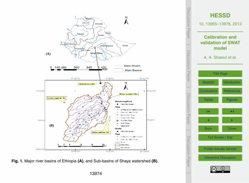
Shaya watershed is found in south-eastern part of Ethiopia in Genale-Dawa basinat the upper most parts of the Weyb basin, located between 6◦ 52′–7◦ 15′ N latitudesand 39◦ 46′–40◦ 02′ E longitudes as shown in Fig. 1. It covers a total drainage area of503.5 km2. The Shaya River originates from the northern flanks of the Bale Mountainsand first flows generally north-eastwards before joining the Weyb river which flows to15

east and south eastwards for the remainder of its course. Finally, it joins with Genaleand Dawa River near Ethiopia–Somalia border to strengthen its journey to Somali low-lands. It originates from an elevation of 4343 m a.s.l., in the Bale Mountains extremepoint locally called Sanetti plateau to an elevation of 2357 m a.s.l at the outlet of thewatershed. The average areal annual rainfall distribution is 1071 mm and the annual20

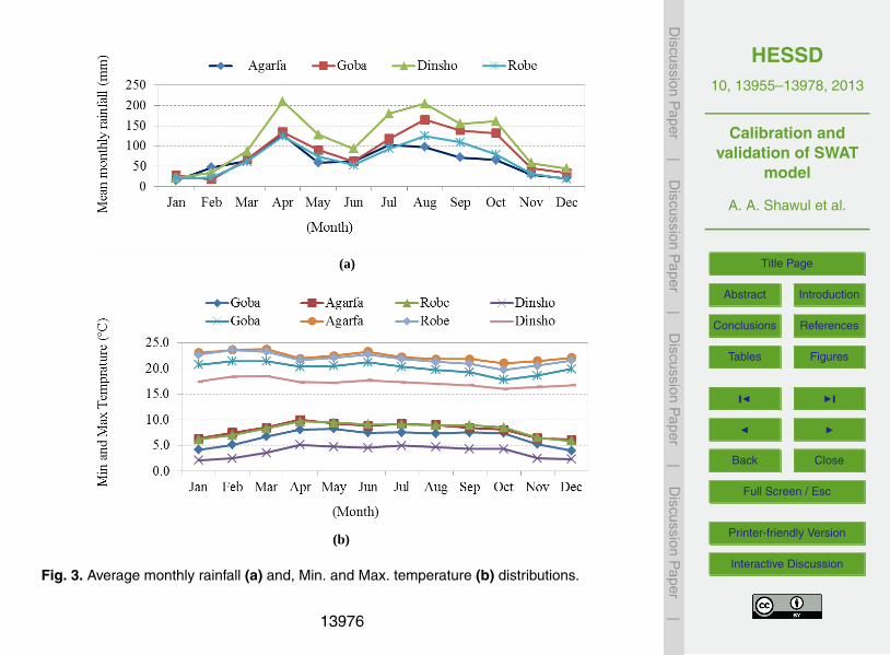
maximum and minimum temperature of the watershed area is about 19.7 ◦C and 6.1 ◦C,respectively.

The Shaya river watershed is a region of rich environmental diversity, but with in-creasing levels of environmental stress in recent years from a rapidly expanding humanpopulation (Farm Africa-SOS Sahel Ethiopia, 2007).25

13958

HESSD10, 13955–13978, 2013

Calibration andvalidation of SWAT

model

A. A. Shawul et al.

Title Page

Abstract Introduction

Conclusions References

Tables Figures

J I

J I

Back Close

Full Screen / Esc

Printer-friendly Version

Interactive Discussion

Discussion

Paper

|D

iscussionP

aper|

Discussion

Paper

|D

iscussionP

aper|

2.2 General description of SWAT model

SWAT is the acronym for Soil and Water Assessment Tool, a river basin scale,continuous-time and spatially distributed model developed for the USDA AgriculturalResearch Service (ARS). It was developed to predict the impact of land managementpractices on water, sediment and agricultural chemical yields in large complex water-5

sheds with varying soils, land use and management conditions over long periods oftime (Neitsch et al., 2005). In recent years, SWAT model has gained international ac-ceptance as a robust interdisciplinary watershed modeling. SWAT is currently appliedworldwide and considered as a versatile model that can be used to integrate multipleenvironmental processes, which support more effective watershed management and10

the development of better informed policy decision (Gassman et al., 2007). The re-view of SWAT model applicability to Ethiopian situations at relatively larger watersheds(Dilnesaw, 2006; Setegn, 2010) indicated that the model is capable of simulating hy-drological processes with a reasonable accuracy. In SWAT, a watershed is divided intomultiple sub-watersheds, which are then further subdivided into hydrologic response15

units (HRUs) that consist of homogeneous land use, management, and soil character-istics (Neitsch et al., 2005). In the land phase of hydrological cycle, SWAT simulatesthe hydrological cycle based on the water balance equation:

SWt = SWo +t∑

i=1

(Rday −Qsurf −Ea −Wseep −Qgw

)(1)

where, SWt is the final soil water content (mm), SWo is the initial soil water content on20

day i (mm), t is the time (days), Rday is the amount of precipitation on day i (mm), Qsurfis the amount of surface runoff on day i (mm), Ea is the amount of evapotranspirationon day i (mm), Wseep is the amount of water entering the vadose zone from the soilprofile on day i (mm), and Qgw is the amount of return flow on day i (mm).

The SCS (Soil Conservation Service) curve number procedure (USDA-SCS, 1972)25

method was used for estimating surface runoff using daily rainfall, SWAT simulates13959

HESSD10, 13955–13978, 2013

Calibration andvalidation of SWAT

model

A. A. Shawul et al.

Title Page

Abstract Introduction

Conclusions References

Tables Figures

J I

J I

Back Close

Full Screen / Esc

Printer-friendly Version

Interactive Discussion

Discussion

Paper

|D

iscussionP

aper|

Discussion

Paper

|D

iscussionP

aper|

surface runoff volumes and peak runoff rates for each HRU. In this study, the SCScurve number method was used to estimate surface runoff. The SCS curve numberequation is:

Qsurf =(Rday −0.2S)2

(Rday +0.8S)(2)

where, Qsurf is the accumulated runoff or rainfall excess (mm), Rday is the rainfall depth5

for the day (mm), S is the retention parameter (mm).SCS defines three antecedent moisture conditions: I – dry (wilting point), II – average

moisture and III – wet (field capacity). The moisture condition I curve number is thelowest value the daily curve number can assume in dry conditions. The curve numbersfor moisture conditions I and III are calculated with the Eqs. (3) and (4), respectively.10

CN1 = CN2 −20× (100−CN2)

(100−CN2 +exp[2.533−0.0636× (100−CN2)])(3)

CN3 = CN2 ×exp[0.00673(100−CN2)] (4)

where CN1 is the moisture condition I curve number, CN2 is the moisture conditionII curve number, and CN3 is the moisture condition III curve number. The retention15

parameter is defined by Eq. (5)

S = 25.4(

1000CN

−10)

(5)

2.3 SWAT model inputs

2.3.1 Digital Elevation Model (DEM)

The DEM forms the base to delineate the watershed boundary, stream network and20

create sub-basins. This was performed by the pre-processing module of the SWAT13960

HESSD10, 13955–13978, 2013

Calibration andvalidation of SWAT

model

A. A. Shawul et al.

Title Page

Abstract Introduction

Conclusions References

Tables Figures

J I

J I

Back Close

Full Screen / Esc

Printer-friendly Version

Interactive Discussion

Discussion

Paper

|D

iscussionP

aper|

Discussion

Paper

|D

iscussionP

aper|

but requires a so-called minimum threshold area. Topography was defined by a DEMwhich describes the elevation of any point in a given area at a specific spatial resolutionas a digital file. It was also used to analyze the drainage patterns of the land surfaceterrain. And sub-basin parameters such as slope, slope length, and defining of thestream network with its characteristics such as channel slope, length, and width were5

derived from the DEM. For this specific study a DEM with a resolution of 30 m wasused, which was sourced from ASTER GDEM official website.

2.3.2 Soil properties

Soils in the study watershed are classified on the basis of the revised FAO/UNESCO-ISWC (FAO/UNESCO-ISWC, 1998) classification system. The soil data was extracted10

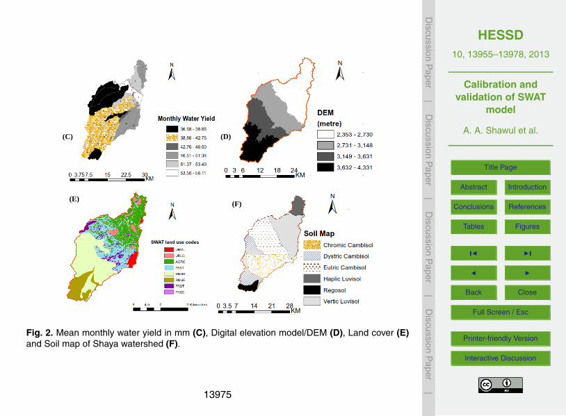
from the 1 : 250000 scale of soil map (Fig. 2) developed by Ministry of Water andEnergy (MoWE) (MoWE, 2007). Basic physico-chemical properties of major soil typesin the watershed were mainly obtained from the following sources: Genale-Dawa riverbasin integrated resources master plan, Soil database and digital soil map from theMoWE produced between the year 2004 and 2007; Soil and Terrain Database for north-15

eastern Africa CD-ROM (FAO, 1998). In addition to these sources, some soil propertieswere estimated based on available soil parameters.

2.3.3 Land Use and Land Cover (LULC) data

The LULC map and all datasets were obtained from (MoWE, 2007). This spatialdatabase was derived from satellite imagery and field data collected between year20

2004 to 2007 (MoWE, 2007) and is the most current and detailed LULC data knownto be available for the study watershed (Fig. 2). The reclassification of the land usemap was made to represent the land use according to the specific LULC types and therespective crop parameter for SWAT database. A lookup table that identifies the SWATland use code for the different categories of LULC was prepared so as to relate the grid25

values to SWAT LULC classes.

13961

HESSD10, 13955–13978, 2013

Calibration andvalidation of SWAT

model

A. A. Shawul et al.

Title Page

Abstract Introduction

Conclusions References

Tables Figures

J I

J I

Back Close

Full Screen / Esc

Printer-friendly Version

Interactive Discussion

Discussion

Paper

|D

iscussionP

aper|

Discussion

Paper

|D

iscussionP

aper|

2.3.4 Meteorological data

The SWAT model requires daily meteorological data that could either be read froma measured data set or be generated by a weather generator model which includeprecipitation, maximum and minimum air temperature, solar radiation, wind speed andrelative humidity. Meteorological data collected from National Meteorological Service5

Agency of Ethiopia (NMSA) for Bale Robe, Dinsho, Agarfa, and Goba stations arewithin the watershed and some are in the vicinity of watershed boundary as shownin Fig. 1. The SWAT weather generator model WXGEN was used to fill missing val-ues in weather data. The Penman–Montheith method which utilizes the solar radia-tion, relative humidity and wind speed data records was employed for estimation of10

potential evapotranspiration (PET) for this specific study. Meteorological stations weregeo-referenced using latitude, longitude, and elevation data.

The typical quality of rainfall data was checked by cross correlation between the sta-tions. The correlation coefficient among the stations on monthly rainfall amount rangedfrom 0.91 to 0.97. This implied a good agreement or consistency of data record on15

the monthly rainfall series of the gauging stations. The climate data for study periodswere finally prepared in .dbf format and imported to the SWAT model database. Meanmonthly rainfall data followed more or less similar trend and patterns as shown onFig. 3.

2.3.5 Hydrological data20

The hydrology of the watershed reflects the rainfall pattern with river flow peaking firstlyin April to May and subsequently in August and October. Daily river discharge data ofthe Shaya River was obtained from the Hydrology Department of the MoWE. It wasused for performing sensitivity analysis, calibration and validation of the SWAT model.

An automated baseflow separation and recession analysis technique (Arnold et al.,25

1999) was employed to separate the baseflow and surface runoff from the total daily

13962

HESSD10, 13955–13978, 2013

Calibration andvalidation of SWAT

model

A. A. Shawul et al.

Title Page

Abstract Introduction

Conclusions References

Tables Figures

J I

J I

Back Close

Full Screen / Esc

Printer-friendly Version

Interactive Discussion

Discussion

Paper

|D

iscussionP

aper|

Discussion

Paper

|D

iscussionP

aper|

streamflow records. This information was then used in order to get SWAT to correctlyreflect basic observed water balance of the watershed.

2.4 Model set up

2.4.1 Watershed delineation

The first step in creating SWAT model input is delineation of the watershed from5

a DEM. Inputs entered into the SWAT model were organized to have spatial char-acteristics. Before going in hand with spatial input data i.e. the soil map, LULC mapand the DEM were projected into the same projection called UTM Zone 37N, whichis a projection parameters for Ethiopia. A watershed was partitioned into a number ofsub-basins, for modeling purposes. The watershed delineation process include five10

major steps, DEM setup, stream definition, outlet and inlet definition, watershed outletsselection and definition and calculation of sub-basin parameters. For the streamdefinition the threshold based stream definition option was used to define the minimumsize of the sub-basins.

15

2.4.2 Hydrological Response Units (HRUs)

The land area in a sub-basin was divided into HRUs. The HRU analysis tool in Arc-SWAT helped to load land use, soil layers and slope map to the project. The delineatedwatershed by ArcSWAT and the prepared land use and soil layers were overlapped100 %. HRU analysis in SWAT includes divisions of HRUs by slope classes in addition20

to land use and soils. The multiple slope option (an option which considers differentslope classes for HRU definition) was selected. The LULC, soil and slope map wasreclassified in order to correspond with the parameters in the SWAT database. Afterreclassifying the land use, soil and slope in SWAT database, all these physical proper-ties were made to be overlaid for HRU definition. For this specific study a 5 % threshold25

13963

HESSD10, 13955–13978, 2013

Calibration andvalidation of SWAT

model

A. A. Shawul et al.

Title Page

Abstract Introduction

Conclusions References

Tables Figures

J I

J I

Back Close

Full Screen / Esc

Printer-friendly Version

Interactive Discussion

Discussion

Paper

|D

iscussionP

aper|

Discussion

Paper

|D

iscussionP

aper|

value for land use, 20 % for soil and 20 % for slope were used. The HRU distribution inthis study was determined by assigning multiple HRU to each sub-basin.

2.4.3 Sensitivity analysis

After a thorough preprocessing of the required input for SWAT model, flow simulationwas performed for an eight years of recording periods starting from 1992 through 1999.5

The first three years of which was used as a warm up period and the simulation wasthen used for sensitivity analysis of hydrologic parameters and for calibration of themodel. The sensitivity analysis was made using a built-in SWAT sensitivity analysistool that uses the Latin Hypercube One-factor-At-a-Time (LH-OAT) (Van Griensven,2005).10

2.4.4 Calibration

Manual and automatic calibration method were applied. First the parameters weremanually calibrated for the period of 1995 to 1999 until the model simulation resultswere acceptable as per the model performance measures. Next, the final parametervalues that were manually calibrated were used as the initial values for the autocal-15

ibration procedure. The graphical and statistical approaches were used to evaluatethe SWAT model performance a number of times until the acceptable values were ob-tained for surface runoff and baseflow independently. The flow calibration proceduremade by SWAT developers in Santhi et al. (2001) and Neitsch et al. (2005) was care-fully followed. SWAT developers assumed an acceptable calibration for hydrology at20

a D ≤ 15%, r2 > 0.6 and ENS > 0.5 (Santhi et al., 2001; Moriasi et al., 2007).

2.4.5 Validation

Streamflow data of three years from 2003 to 2005 were used for validation. The threestatistical model performance measures used in calibration procedure were also usedin validating streamflow.25

13964

HESSD10, 13955–13978, 2013

Calibration andvalidation of SWAT

model

A. A. Shawul et al.

Title Page

Abstract Introduction

Conclusions References

Tables Figures

J I

J I

Back Close

Full Screen / Esc

Printer-friendly Version

Interactive Discussion

Discussion

Paper

|D

iscussionP

aper|

Discussion

Paper

|D

iscussionP

aper|

2.4.6 Model performance evaluation

The regression coefficient (r2) describes the proportion of the total variance in the ob-served data that can be explained by the model. The closer the value of r2 to 1, thehigher is the agreement between the simulated and the measured flow and is calcu-lated as follow:5

r2 =

(∑[Xi −Xav

][Yi − Yav

])2∑[Xi −Xav

]2∑[Yi − Yav

]2(6)

where: Xi is measured value, Xav is average measured value, Yi is simulated value, Yavis average simulated value, the same holds true for Eqs. (7) and (8).

Nash and Sutcliffe simulation efficiency (ENS) indicates the degree of fitness of ob-served and simulated data and given by the following formula.10

ENS = 1−∑

(Xi − Yi )2∑

(Xi −Xav)2(7)

The value of ENS ranges from 1 (best) to negative infinity. If the measured value is thesame as all predictions, ENS is 1. If the ENS is between 0 and 1, it indicates deviationsbetween measured and predicted values. If ENS is negative, predictions are very poor,and the average value of output is a better estimate than the model prediction (Nash15

and Sutcliffe, 1970).The percent difference (D) measures the average difference between the simulated

and measured values for a given quantity over a specified period were calculated asfollows:

D = 100(∑

Yi −∑

Xi∑Xi

)(8)20

A value close to 0 % is best for D. However, higher values for D are acceptable if theaccuracy in which the observed data gathered is relatively poor.

13965

HESSD10, 13955–13978, 2013

Calibration andvalidation of SWAT

model

A. A. Shawul et al.

Title Page

Abstract Introduction

Conclusions References

Tables Figures

J I

J I

Back Close

Full Screen / Esc

Printer-friendly Version

Interactive Discussion

Discussion

Paper

|D

iscussionP

aper|

Discussion

Paper

|D

iscussionP

aper|

3 Results and discussions

3.1 Sensitivity analysis

The model considered twenty seven flow parameters for sensitivity analysis from whichtwenty one of them were found to be relatively sensitive with the category of sensitiv-ity ranging from very high to small. Among the sensitive flow parameters the ground5

water parameters were found to be more sensitive to streamflow. Deep aquifer perco-lation fraction; Rchrg_Dp, Initial curve number (II) value; Cn2, Baseflow alpha factor[days]; Alpha_Bf, Threshold water depth in the shallow aquifer for flow [mm]; Gwqmn,Soil evaporation compensation factor; Esco, Soil depth [mm]; Sol_Z, Threshold wa-ter depth in the shallow aquifer for “revap” [mm]; Revapmin, Maximum potential leaf10

area index; Blai, Available water capacity [(mmwater) (mmsoil)−1]; Sol_Awc, Maximumcanopy storage [mm]; Canmx, Groundwater Delay [days]; Gw_Delay, Saturated hy-draulic conductivity [mmh−1]; Sol_K and Surface runoff lag time [days]; Surlag werefound to be the most effective hydrologic parameters for the simulation of streamflow.A brief description of each hydrologic parameter is listed in the SWAT model user’s15

manual (Neitsch et al., 2005).

3.2 Model calibration

Model calibration followed sensitivity analysis. Calibration for water balance andstreamflow was first done for average annual conditions. After the model was calibratedfor average annual conditions, we shifted into monthly and daily records to fine-tune the20

calibration processes. Model efficiency measures for initial monthly default simulationr2, ENS and D were 0.60, 0.16 and 96.6 respectively which were beyond the acceptableranges. Thus, model parameter adjustments were undertaken for a realistic hydrologicsimulation.

13966

HESSD10, 13955–13978, 2013

Calibration andvalidation of SWAT

model

A. A. Shawul et al.

Title Page

Abstract Introduction

Conclusions References

Tables Figures

J I

J I

Back Close

Full Screen / Esc

Printer-friendly Version

Interactive Discussion

Discussion

Paper

|D

iscussionP

aper|

Discussion

Paper

|D

iscussionP

aper|

The baseflow separation technique indicated about 60 % of the total water yield wascontributed from the subsurface water source which was more than surface runoff in-volvement for the total water yield at the outlet of the watershed.

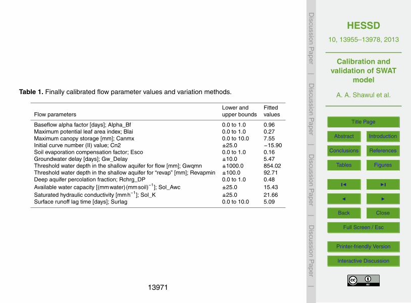
The calibration processes were considered 13 most sensitive flow parameters (Ta-ble 1) and their values were varied iteratively within the allowable ranges until satis-5

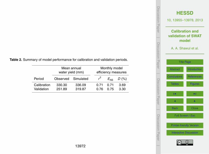
factory agreement between measured and simulated streamflow was obtained. Theautocalibration processes significantly improved model efficiency. The result from dif-ferent statistical method of model performance evaluation met the criteria of ENS > 0.5,r2 > 0.6 and D ≤ ±15%. The statistical results of the model performance for both cali-bration and validation periods on monthly time steps are summarized in Table 2.10

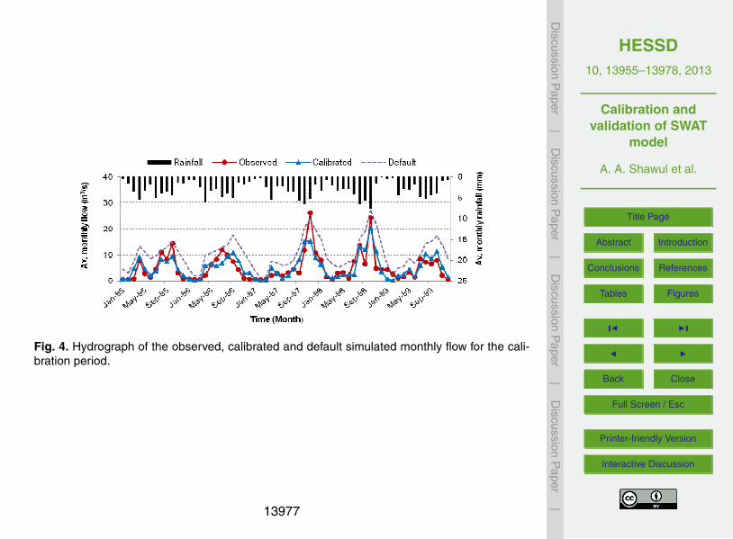
A rigorous hydrologic calibration resulted good SWAT predictive efficiency at themonthly time step of the watershed when compared to measured flow data (Fig. 4).The hydrograph of observed and simulated flow indicated that the SWAT model iscapable of simulating the hydrology of Shaya mountainous watershed. However, themodel was unable to capture some extreme values mainly, observed discharge on the15

month of November 1997 and October 1998. The under prediction of flow during peakevents by the SWAT model has been reported in many studies (Thripati et al., 2003;Gassman et al., 2007; Sathian and Symala, 2009).

3.3 Model validation

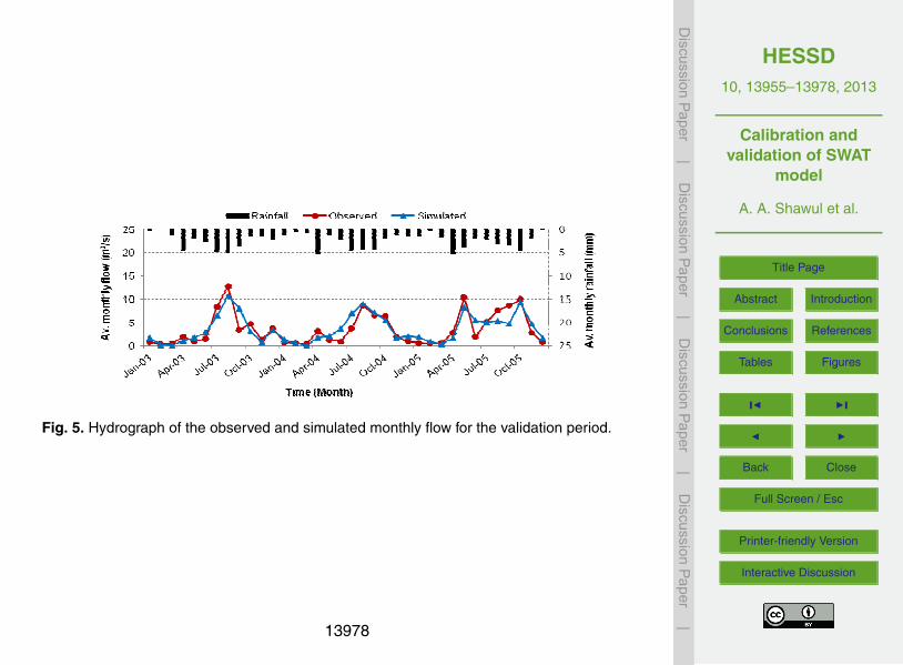
It was found that the model has strong predictive capability with r2, ENS and D values20

of 0.76, 0.75 and 3.30, respectively. Statistical model efficiency criteria fulfilled the re-quirement of r2 > 0.6 and ENS > 0.5 which is recommended by SWAT developer (Santhiet al., 2001). This showed the model parameters represent the processes occurring inthe watershed to the best of their ability given available data and may be used to predictwatershed response for various outputs. The model validation results for monthly flow25

(Fig. 5) indicated generally a good fit between measured and simulated output. Sincethe model performed as well in the validation period, as for the calibration period hence,

13967

HESSD10, 13955–13978, 2013

Calibration andvalidation of SWAT

model

A. A. Shawul et al.

Title Page

Abstract Introduction

Conclusions References

Tables Figures

J I

J I

Back Close

Full Screen / Esc

Printer-friendly Version

Interactive Discussion

Discussion

Paper

|D

iscussionP

aper|

Discussion

Paper

|D

iscussionP

aper|

the set of optimized parameters listed in Table 1 during calibration process for Shayawatershed can be taken as the representative set of parameters for the watershed.

3.4 Monthly and seasonal water yield simulation

The water yield was simulated for the base period of twelve years 1995 to 2006 onmonthly time step at the outlet of Shaya watershed. Moreover, the result was sum-5

marized in a monthly and seasonal bases as comparatively dry (February–May), wet(June–September), intermediate (October–January) and annual bases, after an inten-sive model calibration for a sensitive flow parameters. Mean monthly and annual wateryield simulated for a base period found to be 25.8 mm and 309.0 mm, respectively.Seasonal water yield simulation resulted 56.6 mm, 89.7 mm and 155.0 mm for dry, in-10

termediate and wet seasons respectively. It indicated that the south-western part of thewatershed has a larger contribution to the total water yield of the watershed.

3.5 Average annual water balance components of the watershed

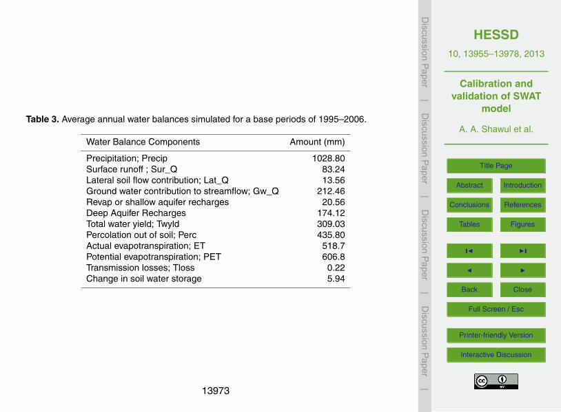
The SWAT model estimated other relevant water balance components in addition tothe daily and monthly discharge of the watershed. Average annual basin values for15

different water balance components during a base simulation periods shows averageannual watershed gain and losses with change in soil water storage Table 3. Fromthese components actual evapotranspiration contributed a larger amount of water lossfrom the watershed and total water yield is the amount of streamflow leaving the outletof watershed during the time step.20

4 Conclusion

Understandings on hydrological processes and develop suitable models for a water-shed is the most important aspect in water resource development and managementprogrammes. Watershed based hydrologic simulation models are likely to be used for

13968

HESSD10, 13955–13978, 2013

Calibration andvalidation of SWAT

model

A. A. Shawul et al.

Title Page

Abstract Introduction

Conclusions References

Tables Figures

J I

J I

Back Close

Full Screen / Esc

Printer-friendly Version

Interactive Discussion

Discussion

Paper

|D

iscussionP

aper|

Discussion

Paper

|D

iscussionP

aper|

the assessment of the quantity and quality of water. The performance and applicabilityof SWAT model was successfully evaluated through sensitivity analysis, model calibra-tion and validation. Subsurface flow parameters were found to be more sensitive to thestreamflow of the watershed, signifying the watershed is rich in ground water as a resultof good recharge capacity. SWAT model was found to produce a reliable estimate of5

monthly runoff for Shaya watershed which was confirmed by various model efficiencymeasures. Therefore, the calibrated parameter values can be considered for further hy-drologic simulation of the watershed. The model can also be taken as a potential toolfor simulation of the hydrology of unguaged watershed in mountainous areas, whichbehave hydro-meteorologically similar with Shaya watershed. However, for a more ac-10

curate modeling of hydrology, a large effort will be required to improve the quality ofavailable input data. Future studies on Shaya watershed modeling should address theissues related to water quality and evaluate best management practices to addressdifferent watershed management issues.

References15

Arnold, J. G. and Allen, P. M.: Automated methods for estimating baseflow and ground waterrecharge from stream flow records, J. Am. Water Resour. Assoc., 35, 411–424, 1999.

Arnold, J. G., Srinivasan, R., Muttiah, R. R., and Williams, J. R.: Large area hydrologic modelingand assessment part I: model development, J. Am. Water Resour. Assoc., 34, 73–89, 1998.

Dilnesaw, A.: Modeling of hydrology and soil erosion of Upper Awash River Basin, Ph.D. Dis-20

sertation, University of Bonn, Bonn, Germany, 236 pp., 2006.FAO: The Soil and Terrain Database for northeastern Africa (CDROM), FAO, Rome, 1998.FAO/UNESCO-ISWC: The World Reference Base for Soil Resources, Rome, Italy, 1998.Farm Africa-SOS Sahel Ethiopia: Participatory Natural Resource Management Programme

and Oromia Bureau of Agriculture and Rural Development, Six Months Report, Bale Robe,25

Ethiopia, 45 pp., 2007.Gassman, W. P., Reyes, M. R., Green, C. H., and Arnold, J. G.: SWAT peer-reviewed literature:

a review, Proceedings of the 3rd International SWAT conference, Zurich, 11–15 July, 1–18,2005.

13969

HESSD10, 13955–13978, 2013

Calibration andvalidation of SWAT

model

A. A. Shawul et al.

Title Page

Abstract Introduction

Conclusions References

Tables Figures

J I

J I

Back Close

Full Screen / Esc

Printer-friendly Version

Interactive Discussion

Discussion

Paper

|D

iscussionP

aper|

Discussion

Paper

|D

iscussionP

aper|

Gassman, W. P., Reyes, M. R., Green, C. H., and Arnold, J. G.: The soil and water assessmenttool: historical development, applications, and future research direction, T. ASABE, 50, 1211–1250, 2007.

McCornick, P. G., Kamara, A. B., and Girma, T. (Eds.): Integrated water and landmanagement research and capacity building priorities for Ethiopia, Proceedings of a5

MoWR/EARO/IWMI/ILRI international workshop held at ILRI, Addis Ababa, Ethiopia, 2–4 De-cember 2002, IWMI, Colombo, Sri Lanka, and ILRI, Nairobi, Kenya, 267 pp., 2003.

Moriasi, D. N, Arnold, J. G., Van Liew, M. W., Bingner, R. L., Harem, R. D., and Veith, T. L.: Modelevaluation guidelines for systematic quantification of accuracy in watershed simulations, T.ASABE, 50, 850–900, 2007.10

MoWE: Genale-Dawa River Basin Integrated Resources Development Master plan Study, Sec-tor Reports, Addis Ababa, Ethiopia, 2007.

Nash, J. E. and Sutcliff, J. V.: River flow forecasting through conceptual models, part I – a dis-cussion of principles, J. Hydrol., 10, 282–290, 1970.

Neitsch, S. I., Arnold, J. G., Kinrv, J. R., and Williams, J. R.: Soil and Water Assessment Tool,15

Theoretical Documentation, Version 2005, USDA Agricultural Research Service Texas A andM Black land Research Center, Temple, TX, 2005.

Sanjay, K., Jaivir T., and Vishal, S.: Simulation of runoff and sediment yield for a Himalayanwatershed using SWAT model, J. Water Res. Protect., 2, 267–281, 2010.

Santhi, C., Arnold, J. G., Williams, J. R., Dugas, W. A., Srinivasan, R., and Hauck, L. M.: Valida-20

tion of the SWAT model on a large river basin with point and nonpoint sources, J. Am. WaterResour. Assoc., 37, 1169–1188, 2001.

Sathian, K. and Symala, P.: Application of GIS integrated SWAT model for basin level waterbalance, Indian J. Soil Cons., 37, 100–105, 2009.

Setegn, S.: Modeling hydrological and hydrodynamic processes in Lake Tana Basin, Ethiopia,25

KTH, TRITA-LWR, Ph.D. Dissertation, 74 pp., 2010.Tripathi, M. P., Panda, R. K., and Raghuwanshi, N. S.: Identification and prioritization of critical

sub-watersheds for soil conservation management using the SWAT model, Biosyst. Eng.,85, 365–379, 2003.

USDA Soil Conservation Service (SCS): National Engineering Handbook, Section 4: Hydrology,30

Chaps. 4–10, 1972.Van Griensven, A.: Sensitivity, auto-calibration, uncertainty and model evaluation in SWAT

2005, UNESCO-IHE, 48 pp., 2005.

13970

HESSD10, 13955–13978, 2013

Calibration andvalidation of SWAT

model

A. A. Shawul et al.

Title Page

Abstract Introduction

Conclusions References

Tables Figures

J I

J I

Back Close

Full Screen / Esc

Printer-friendly Version

Interactive Discussion

Discussion

Paper

|D

iscussionP

aper|

Discussion

Paper

|D

iscussionP

aper|

Table 1. Finally calibrated flow parameter values and variation methods.

Lower and FittedFlow parameters upper bounds values

Baseflow alpha factor [days]; Alpha_Bf 0.0 to 1.0 0.96Maximum potential leaf area index; Blai 0.0 to 1.0 0.27Maximum canopy storage [mm]; Canmx 0.0 to 10.0 7.55Initial curve number (II) value; Cn2 ±25.0 −15.90Soil evaporation compensation factor; Esco 0.0 to 1.0 0.16Groundwater delay [days]; Gw_Delay ±10.0 5.47Threshold water depth in the shallow aquifer for flow [mm]; Gwqmn ±1000.0 854.02Threshold water depth in the shallow aquifer for “revap” [mm]; Revapmin ±100.0 92.71Deep aquifer percolation fraction; Rchrg_DP 0.0 to 1.0 0.48Available water capacity [(mmwater) (mmsoil)−1]; Sol_Awc ±25.0 15.43Saturated hydraulic conductivity [mmh−1]; Sol_K ±25.0 21.66Surface runoff lag time [days]; Surlag 0.0 to 10.0 5.09

13971

HESSD10, 13955–13978, 2013

Calibration andvalidation of SWAT

model

A. A. Shawul et al.

Title Page

Abstract Introduction

Conclusions References

Tables Figures

J I

J I

Back Close

Full Screen / Esc

Printer-friendly Version

Interactive Discussion

Discussion

Paper

|D

iscussionP

aper|

Discussion

Paper

|D

iscussionP

aper|

Table 2. Summary of model performance for calibration and validation periods.

Mean annual Monthly modelwater yield (mm) efficiency measures

Period Observed Simulated r2 ENS D (%)

Calibration 330.30 336.09 0.71 0.71 3.69Validation 251.89 319.87 0.76 0.75 3.30

13972

HESSD10, 13955–13978, 2013

Calibration andvalidation of SWAT

model

A. A. Shawul et al.

Title Page

Abstract Introduction

Conclusions References

Tables Figures

J I

J I

Back Close

Full Screen / Esc

Printer-friendly Version

Interactive Discussion

Discussion

Paper

|D

iscussionP

aper|

Discussion

Paper

|D

iscussionP

aper|

Table 3. Average annual water balances simulated for a base periods of 1995–2006.

Water Balance Components Amount (mm)

Precipitation; Precip 1028.80Surface runoff ; Sur_Q 83.24Lateral soil flow contribution; Lat_Q 13.56Ground water contribution to streamflow; Gw_Q 212.46Revap or shallow aquifer recharges 20.56Deep Aquifer Recharges 174.12Total water yield; Twyld 309.03Percolation out of soil; Perc 435.80Actual evapotranspiration; ET 518.7Potential evapotranspiration; PET 606.8Transmission losses; Tloss 0.22Change in soil water storage 5.94

13973

HESSD10, 13955–13978, 2013

Calibration andvalidation of SWAT

model

A. A. Shawul et al.

Title Page

Abstract Introduction

Conclusions References

Tables Figures

J I

J I

Back Close

Full Screen / Esc

Printer-friendly Version

Interactive Discussion

Discussion

Paper

|D

iscussionP

aper|

Discussion

Paper

|D

iscussionP

aper|

Fig. 1. Major river basins of Ethiopia (A), and Sub-basins of Shaya watershed (B)

(A)

(B)

Fig. 1. Major river basins of Ethiopia (A), and Sub-basins of Shaya watershed (B).

13974

HESSD10, 13955–13978, 2013

Calibration andvalidation of SWAT

model

A. A. Shawul et al.

Title Page

Abstract Introduction

Conclusions References

Tables Figures

J I

J I

Back Close

Full Screen / Esc

Printer-friendly Version

Interactive Discussion

Discussion

Paper

|D

iscussionP

aper|

Discussion

Paper

|D

iscussionP

aper|

Fig. 2. Mean monthly water yield in mm (C), Digital elevation model/DEM (D), Land cover (E) and Soil map of Shaya watershed (F).

(C) (D)

(F) (E)

Fig. 2. Mean monthly water yield in mm (C), Digital elevation model/DEM (D), Land cover (E)and Soil map of Shaya watershed (F).

13975

HESSD10, 13955–13978, 2013

Calibration andvalidation of SWAT

model

A. A. Shawul et al.

Title Page

Abstract Introduction

Conclusions References

Tables Figures

J I

J I

Back Close

Full Screen / Esc

Printer-friendly Version

Interactive Discussion

Discussion

Paper

|D

iscussionP

aper|

Discussion

Paper

|D

iscussionP

aper|

(a)

(b)

Fig. 3. Average monthly rainfall (a) and, Min. and Max. temperature (b) distributions. Fig. 3. Average monthly rainfall (a) and, Min. and Max. temperature (b) distributions.

13976

HESSD10, 13955–13978, 2013

Calibration andvalidation of SWAT

model

A. A. Shawul et al.

Title Page

Abstract Introduction

Conclusions References

Tables Figures

J I

J I

Back Close

Full Screen / Esc

Printer-friendly Version

Interactive Discussion

Discussion

Paper

|D

iscussionP

aper|

Discussion

Paper

|D

iscussionP

aper|

Figure 3. Average monthly rainfall distributions in Shaya river watershed.

Figure 4. Hydrograph of the observed, calibrated and default simulated monthly flow for the calibration period.

Figure 5. Hydrograph of the observed and simulated monthly flow for the validation period.

Fig. 4. Hydrograph of the observed, calibrated and default simulated monthly flow for the cali-bration period.

13977

HESSD10, 13955–13978, 2013

Calibration andvalidation of SWAT

model

A. A. Shawul et al.

Title Page

Abstract Introduction

Conclusions References

Tables Figures

J I

J I

Back Close

Full Screen / Esc

Printer-friendly Version

Interactive Discussion

Discussion

Paper

|D

iscussionP

aper|

Discussion

Paper

|D

iscussionP

aper|

Figure 3. Average monthly rainfall distributions in Shaya river watershed.

Figure 4. Hydrograph of the observed, calibrated and default simulated monthly flow for the calibration period.

Figure 5. Hydrograph of the observed and simulated monthly flow for the validation period.

Fig. 5. Hydrograph of the observed and simulated monthly flow for the validation period.

13978