
Calculus.pdf
140
Introduction Functions Course Plan Introduction Functions Differentiation Integration Applications Discretization Conclusion JuSaK CalculusI
Transcript of Calculus.pdf

Introduction Functions
Course Plan
IntroductionFunctionsDifferentiationIntegrationApplicationsDiscretizationConclusion
JuSaK CalculusI

Introduction Functions
Course Plan
IntroductionFunctionsDifferentiationIntegrationApplicationsDiscretizationConclusion
JuSaK CalculusI
Introduction Functions
Outline
1 IntroductionFunctions
JuSaK CalculusI

Functions
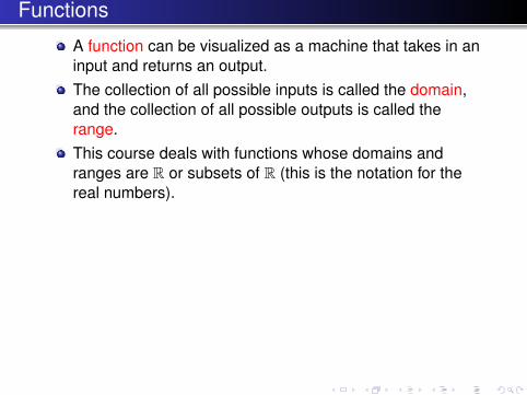
A function can be visualized as a machine that takes in aninput and returns an output.The collection of all possible inputs is called the domain,and the collection of all possible outputs is called therange.This course deals with functions whose domains andranges are R or subsets of R (this is the notation for thereal numbers).

Functions
A function can be visualized as a machine that takes in aninput and returns an output.The collection of all possible inputs is called the domain,and the collection of all possible outputs is called therange.This course deals with functions whose domains andranges are R or subsets of R (this is the notation for thereal numbers).

Functions
Example1 Polynomials, e.g. f (x) = x3 − 5x2 + x + 9. Give the domain
and range of f .2 Trigonometric functions, e.g. sin, cos, tan. Give the domain
and range for each of these.3 Exponential function, ex. Give the domain and range for the
exponential.4 The natural logarithm function, ln x. Recall that this is the
inverse of the exponential function. Give the domain andrange for ln x.
5 Is sin−1 a function? If so, why? If not, is there a way tomake it into a function?

Operations of Functions
Definition (Composition)The composition of two functions, f and g, is defined to be thefunction that takes as its input x and returns as its output g(x)fed into f .
f ◦ g(x) = f (g(x)).
Example
1√
1− x2can be thought of as the composition of twofunctions, f and g. If g = 1− x2, f would be the function thattakes an input g(x) and returns its square root.
2 Compute the composition f ◦ f , i.e. the composition of fwith itself, where f (x) = 1
x+1 .

Operations of Functions
Definition (Inverse)
The inverse is the that undoes f . If you plug f (x) into f−1, youwill get x. Notice that this function works both ways. If you plugf−1(x) into f (x), you will get back x again.
f−1(f (x)) = x , f (f−1(x)) = x.
NOTE: f−1 denotes the inverse, not the reciprocal: f−1 6= 1f (x) .
Section 6.2 Inverse Functions 487
6.2 INVERSE FUNCTIONS
The notion of an inverse relationship is basic to many areas of science, although the termis only infrequently used. The number of common inverse problems is immense. As onlyone example, take the case of the electrocardiogram (EKG). In an EKG, technicians con-nect a series of electrodes to a patient’s chest and use measurements of electrical activityon the surface of the body to infer something about the electrical activity on the surface ofthe heart. This is referred to as an inverse problem, since physicians are attempting to de-termine what inputs (i.e., the electrical activity on the surface of the heart) cause an ob-served output (the measured electrical activity on the surface of the chest).
The mathematical notion of inverse is much the same as that described above. Givenan output (i.e., a value in the range of a given function), we wish to find the input (the valuein the domain) that produced the observed output. That is, given a y ∈ Range{ f }, find thex ∈ Domain{ f } for which y = f (x). (See the illustration of the inverse function g(x)
shown in Figure 6.3.)For instance, suppose that f (x) = x3 and y = 8. Can you find an x such that x3 = 8?
That is, can you find the x-value corresponding to y = 8 (see Figure 6.4)? Of course,you know the solution of this particular equation: x = 3
√8 = 2. In fact, in general, if
x3 = y, then x = 3√
y. In light of this, we say that the cube root function is the inverse off (x) = x3.
If f (x) = x3 and g(x) = x1/3, show that
f (g(x)) = x and g( f (x)) = x,
for all x .
Solution For all real numbers x, we have
f (g(x)) = f (x1/3) = (x1/3)3 = x
and
g( f (x)) = g(x3) = (x3)1/3 = x .
■
Notice in example 2.1 that the action of f undoes the action of g and vice versa. Wemay take this as the definition of an inverse function. More precisely, we have the follow-ing definition.
Observe that many familiar functions have no inverse.
Definition 2.1
Assume that f and g have domains A and B, respectively, and that f (g(x)) is definedfor all x ∈ B and g( f (x)) is defined for all x ∈ A. If
f (g(x)) = x, for all x ∈ B and
g( f (x)) = x, for all x ∈ A,
we say that g is the inverse of f, written g = f −1. Equivalently, f is the inverse of g,
f = g−1.
Two Functions That Reverse the Action of Each OtherExample 2.1
f (x)
g(x)
x
Domain { f}
y
Range { f}
Figure 6.3
g(x) = f −1(x).
y
x
8
4
2
�2
6
21�2
y � x3
Figure 6.4
Finding the x-value correspondingto y = 8.
C A U T I O N
Pay close attention to the notation.Notice that f −1(x ) does not mean
1
f (x ). We write the reciprocal of
f (x ) as:
1
f (x )= [ f (x )]−1.
smi98485_ch06a.qxd 5/17/01 1:26 PM Page 487
g(x) = f−1(x)

Inverse Functions
Example
Let’s consider f (x) = x3. Its inverse is f−1(x) = x1/3.
f−1(f (x)) = (x3)1/3 = x , f (f−1(x)) = (x1/3)3 = x.
In example 2.5, we saw a function that we knew had an inverse, although we could notfind that inverse algebraically. Even when we can’t find an inverse function explicitly, wecan say something graphically. Notice that if (a, b) is a point on the graph of y = f (x) andf has an inverse, f −1, then since
b = f (a),
we have that
f −1(b) = f −1( f (a)) = a.
That is, (b, a) is a point on the graph of y = f −1(x). This tells us a great deal about the in-verse function. In particular, we can immediately obtain any number of points on the graphof y = f −1(x), simply by inspection. Further, notice that the point (b, a) is the reflectionof the point (a, b) through the line y = x (see Figure 6.10). It now follows that given thegraph of any one-to-one function, you can draw the graph of its inverse simply by reflect-ing the entire graph through the line y = x . One consequence of this symmetry is thefollowing result.
In the following example, we illustrate the symmetry of a function and its inverse.
Draw a graph of f (x) = x3 and its inverse.
Solution From example 2.1, the inverse of f (x) = x3 is f −1(x) = x1/3. Noticethe symmetry of their graphs shown in Figure 6.11.
■
Observe that we can use this symmetry principle to draw the graph of an inverse func-tion, even when we don’t have a formula for that function (see Figure 6.12).
Draw a graph of f (x) = x5 + 8x3 + x + 1 and its inverse.
Solution In example 2.5, we showed that f was strictly increasing and hence, wasone-to-one, but we were unable to find a formula for the inverse function. Despite this,we can draw a graph of f −1 with ease. One way to do this would be to plot a few pointson the graph of y = f −1(x) by hand, but we suggest that you use the parametric plot-ting feature of your graphing utility. To write down parametric equations for the curvey = f (x), we introduce the parameter t and observe that
x = t and y = f (t) (2.1)
are parametric equations for y = f (x). Notice that parametric equations for y = f −1(x)
are then simply
x = f (t) and y = t. (2.2)
Drawing the Graph of an Unknown Inverse FunctionExample 2.7
The Graph of a Function and Its InverseExample 2.6
Theorem 2.2
Suppose that f is a one-to-one and continuous function. Then, f −1 is also continuous.
490 Chapter 6 Exponentials, Logarithms and Other Transcendental Functions
y
x
�1
1
1�1
y � x
y � x3
y � x1/3
Figure 6.11
y = x3 and y = x1/3.
y
x
y � f (x)
y � f �1(x)
y � x
Figure 6.12
Graph of f and f −1.
y
xab
a
b
y � x
(b, a)
(a, b)
Figure 6.10
Reflection through y = x .
smi98485_ch06a.qxd 5/17/01 1:26 PM Page 490

Inverse Functions
Notice that the graphs of f and f−1 are always going to besymmetric about the line y = x. That is the line where the inputand the output are the same.
In example 2.5, we saw a function that we knew had an inverse, although we could notfind that inverse algebraically. Even when we can’t find an inverse function explicitly, wecan say something graphically. Notice that if (a, b) is a point on the graph of y = f (x) andf has an inverse, f −1, then since
b = f (a),
we have that
f −1(b) = f −1( f (a)) = a.
That is, (b, a) is a point on the graph of y = f −1(x). This tells us a great deal about the in-verse function. In particular, we can immediately obtain any number of points on the graphof y = f −1(x), simply by inspection. Further, notice that the point (b, a) is the reflectionof the point (a, b) through the line y = x (see Figure 6.10). It now follows that given thegraph of any one-to-one function, you can draw the graph of its inverse simply by reflect-ing the entire graph through the line y = x . One consequence of this symmetry is thefollowing result.
In the following example, we illustrate the symmetry of a function and its inverse.
Draw a graph of f (x) = x3 and its inverse.
Solution From example 2.1, the inverse of f (x) = x3 is f −1(x) = x1/3. Noticethe symmetry of their graphs shown in Figure 6.11.
■
Observe that we can use this symmetry principle to draw the graph of an inverse func-tion, even when we don’t have a formula for that function (see Figure 6.12).
Draw a graph of f (x) = x5 + 8x3 + x + 1 and its inverse.
Solution In example 2.5, we showed that f was strictly increasing and hence, wasone-to-one, but we were unable to find a formula for the inverse function. Despite this,we can draw a graph of f −1 with ease. One way to do this would be to plot a few pointson the graph of y = f −1(x) by hand, but we suggest that you use the parametric plot-ting feature of your graphing utility. To write down parametric equations for the curvey = f (x), we introduce the parameter t and observe that
x = t and y = f (t) (2.1)
are parametric equations for y = f (x). Notice that parametric equations for y = f −1(x)
are then simply
x = f (t) and y = t. (2.2)
Drawing the Graph of an Unknown Inverse FunctionExample 2.7
The Graph of a Function and Its InverseExample 2.6
Theorem 2.2
Suppose that f is a one-to-one and continuous function. Then, f −1 is also continuous.
490 Chapter 6 Exponentials, Logarithms and Other Transcendental Functions
y
x
�1
1
1�1
y � x
y � x3
y � x1/3
Figure 6.11
y = x3 and y = x1/3.
y
x
y � f (x)
y � f �1(x)
y � x
Figure 6.12
Graph of f and f −1.
y
xab
a
b
y � x
(b, a)
(a, b)
Figure 6.10
Reflection through y = x .
smi98485_ch06a.qxd 5/17/01 1:26 PM Page 490
We used the two pairs of parametric equations (2.1) and (2.2) to produce the graphs ofy = f (x) and y = f −1(x) shown in Figure 6.13. We also added a dashed line for theline y = x, entered parametrically as
x = t and y = t.
■
We make one final observation regarding inverse functions. Suppose that f is a one-to-one and differentiable function. Then, as a consequence of the symmetry of the functionand its inverse, notice that, as long as f ′( f −1(a)) �= 0 (i.e., the tangent line is not horizon-tal), then f −1(x) should be differentiable at x = a (the tangent line to f −1(x) is not verti-cal). We express this notion carefully in the following theorem.
Let g(x) = f −1(x). Then for any fixed x = a, we have from the alternative definitionof derivative that
g′(a) = limx→a
g(x) − g(a)
x − a. (2.3)
Since g = f −1, we have that y = g(x) if and only if f (y) = x and b = g(a) if andonly if f (b) = a. Further, since f is differentiable, it is continuous and so, from Theo-rem 2.2, g must be continuous, also. In particular, this says that as x → a, we must alsohave g(x) → g(a), so that y → b. From (2.3), we now have
g′(a) = limx→a
g(x) − g(a)
x − a= lim
y→b
y − b
f (y) − f (b)
= limy→b
1f (y) − f (b)
y − b
= 1
limy→b
f (y) − f (b)
y − b
= 1
f ′(b)
= 1
f ′( f −1(a)),
as desired, since the limit in the denominator is nonzero.
■
As an alternative to the proof of Theorem 2.3 given above, if we know that an inversefunction is differentiable, we can find its derivative using implicit differentiation, as fol-lows. If y = f −1(x), then
f (y) = x . (2.4)
Differentiating both sides of (2.4) with respect to x, we find that
d
dxf (y) = d
dxx,
Proof
Theorem 2.3
Suppose that f is a one-to-one and differentiable function. Then, as long asf ′( f −1(x)) �= 0,
d
dxf −1(x) = 1
f ′( f −1(x)).
Section 6.2 Inverse Functions 491
y
x
�1
1
1�1
y � f (x)
y � f �1(x)
y � x
Figure 6.13
Graph of f and f −1.
N O T E S
Notice that Theorem 2.3 says thatthe slope of the tangent line toy = f −1(x ) at a point (a, b) issimply the reciprocal of the slope ofthe tangent line to y = f (x ) at themirror image point (b, a).
smi98485_ch06a.qxd 5/17/01 1:26 PM Page 491

Classes of Functions
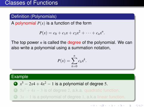
Definition (Polynomials)
A polynomial P(x) is a function of the form
P(x) = c0 + c1x + c2x2 + · · ·+ cnxn.
The top power n is called the degree of the polynomial. We canalso write a polynomial using a summation notation,
P(x) =n∑
k=0
ckxk.
Example1 x5 − 2x4 + 4x2 − 1 is a polynomial of degree 5.2 5x2 + 4x− 3 is of degree 2, a.k.a. quadratic function.3 3x− 1 is a polynomial of degree 1, a.k.a linear function.

Classes of Functions
Definition (Polynomials)
A polynomial P(x) is a function of the form
P(x) = c0 + c1x + c2x2 + · · ·+ cnxn.
The top power n is called the degree of the polynomial. We canalso write a polynomial using a summation notation,
P(x) =n∑
k=0
ckxk.
Example1 x5 − 2x4 + 4x2 − 1 is a polynomial of degree 5.2 5x2 + 4x− 3 is of degree 2, a.k.a. quadratic function.3 3x− 1 is a polynomial of degree 1, a.k.a linear function.

Classes of Functions
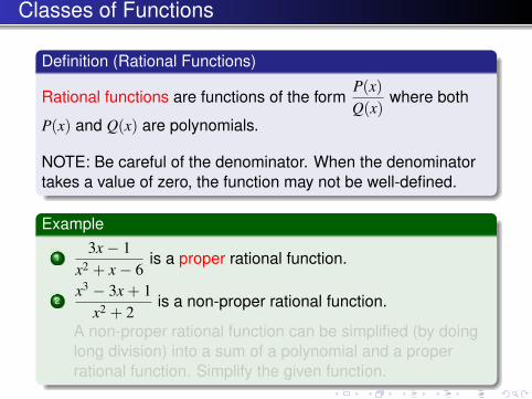
Definition (Rational Functions)
Rational functions are functions of the formP(x)Q(x)
where both
P(x) and Q(x) are polynomials.
NOTE: Be careful of the denominator. When the denominatortakes a value of zero, the function may not be well-defined.
Example
13x− 1
x2 + x− 6is a proper rational function.
2x3 − 3x + 1
x2 + 2is a non-proper rational function.
A non-proper rational function can be simplified (by doinglong division) into a sum of a polynomial and a properrational function. Simplify the given function.

Classes of Functions
Definition (Rational Functions)
Rational functions are functions of the formP(x)Q(x)
where both
P(x) and Q(x) are polynomials.
NOTE: Be careful of the denominator. When the denominatortakes a value of zero, the function may not be well-defined.
Example
13x− 1
x2 + x− 6is a proper rational function.
2x3 − 3x + 1
x2 + 2is a non-proper rational function.
A non-proper rational function can be simplified (by doinglong division) into a sum of a polynomial and a properrational function. Simplify the given function.

Classes of Functions
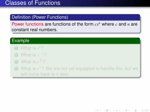
Definition (Power Functions)Power functions are functions of the form cxn where c and n areconstant real numbers.
Example1 What is x0?2 What is x−
12 ?
3 What is x227 ?
4 What is xπ? We are not yet equipped to handle this, but wewill come back to it later.
Classes of Functions
Definition (Power Functions)Power functions are functions of the form cxn where c and n areconstant real numbers.
Example1 What is x0?2 What is x−
12 ?
3 What is x227 ?
4 What is xπ? We are not yet equipped to handle this, but wewill come back to it later.

Classes of Functions
Definition (Power Functions)Power functions are functions of the form cxn where c and n areconstant real numbers.
Example1 What is x0?2 What is x−
12 ?
3 What is x227 ?
4 What is xπ? We are not yet equipped to handle this, but wewill come back to it later.

Classes of Functions
Definition (Power Functions)Power functions are functions of the form cxn where c and n areconstant real numbers.
Example1 What is x0?2 What is x−
12 ?
3 What is x227 ?
4 What is xπ? We are not yet equipped to handle this, but wewill come back to it later.

Classes of Functions
Definition (Power Functions)Power functions are functions of the form cxn where c and n areconstant real numbers.
Example1 What is x0?2 What is x−
12 ?
3 What is x227 ?
4 What is xπ? We are not yet equipped to handle this, but wewill come back to it later.

Classes of Functions
Definition (Power Functions)Power functions are functions of the form cxn where c and n areconstant real numbers.
Example1 What is x0?2 What is x−
12 ?
3 What is x227 ?
4 What is xπ? We are not yet equipped to handle this, but wewill come back to it later.

Classes of Functions
DefinitionA function f is periodic of period T if
f (x + T) = f (x)
for all x such that x and x + T are in the domain of f . Thesmallest number T > 0 is called the fundamental period.
RemarkUnless otherwise noted, we always measure angles in radians.
Degrees 0◦ 30◦ 45◦ 60◦ 90◦ 135◦ 180◦ 270◦ 360◦
Radians 0 π6
π4
π3
π2
3π4 π 3π
2 2π
π 6= 180, π = 3.1415 . . .

Classes of Functions
Theoremf (θ) = sin θ and f (θ) = cos θ are periodic, of period 2π.
Exercise (Trigonometric Functions)1 What are the definitions of sin and cos.2 Sketch the graph of y = sin x and y = cos x.
Pythagorean identity of trigonometric functions:

Classes of Functions
The functions cos θ and sin θ returns the x and y coordinates,respectively, of a point on the unit circle with angle θ to thex-axis:

Trigonometric Functions
x sin x cos x0 0 1π6
12
√3
2π4
√2
2
√2
2π3
√3
212
π2 1 0
2π3
√3
2 − 12
3π4
√2
2 −√
22
5π6
12 −
√3
2π 0 −13π2 −1 0
2π 0 1
42 Chapter 0 Preliminaries
Since a complete circle is 2π radians, adding 2π to any angle takes you all the wayaround the circle and back to the same point (x, y). This says that
sin(θ + 2π) = sin θ
and
cos(θ + 2π) = cos θ,
for all values of θ.
You are likely already familiar with the graphs of f (x) = sin x and g(x) = cos xshown in Figures 0.48a and 0.48b, respectively.
Proof
y
�1
1
q w�w r�r �qx
Figure 0.48a
y = sin x .
y
�1
1
p 2p�2p �px
Figure 0.48b
y = cos x .
Notice that you could slide the graph of y = sin x slightly to the left or right and get anexact copy of the graph of y = cos x . Specifically, you might observe that
You should also observe from Figure 0.47 that the Pythagorean Theorem gives us thefamiliar identity
since the hypotenuse of the indicated triangle is 1. This holds for any angle θ.
Instead of writing (sin θ)2 or (cos θ)2, we usually use the notation sin2 θ and cos2 θ, respectively.
The accompanying table lists some common values of sine and cosine. Notice thatmany of these can be read directly from Figure 0.47.
Remark 5.2
sin2 θ + cos2 θ = 1,
sin(
x + π
2
)= cos x .
x sin x cos x
0 0 1
π
612
√3
2
π4
√2
2
√2
2
π3
√3
212
π2 1 0
2π3
√3
2 − 12
3π4
√2
2 −√
22
5π6
12 −
√3
2
π 0 −1
3π2 −1 0
2π 0 1
smi98485_ch00b.qxd 5/17/01 10:46 AM Page 42
y = sin x
42 Chapter 0 Preliminaries
Since a complete circle is 2π radians, adding 2π to any angle takes you all the wayaround the circle and back to the same point (x, y). This says that
sin(θ + 2π) = sin θ
and
cos(θ + 2π) = cos θ,
for all values of θ.
You are likely already familiar with the graphs of f (x) = sin x and g(x) = cos xshown in Figures 0.48a and 0.48b, respectively.
Proof
y
�1
1
q w�w r�r �qx
Figure 0.48a
y = sin x .
y
�1
1
p 2p�2p �px
Figure 0.48b
y = cos x .
Notice that you could slide the graph of y = sin x slightly to the left or right and get anexact copy of the graph of y = cos x . Specifically, you might observe that
You should also observe from Figure 0.47 that the Pythagorean Theorem gives us thefamiliar identity
since the hypotenuse of the indicated triangle is 1. This holds for any angle θ.
Instead of writing (sin θ)2 or (cos θ)2, we usually use the notation sin2 θ and cos2 θ, respectively.
The accompanying table lists some common values of sine and cosine. Notice thatmany of these can be read directly from Figure 0.47.
Remark 5.2
sin2 θ + cos2 θ = 1,
sin(
x + π
2
)= cos x .
x sin x cos x
0 0 1
π
612
√3
2
π4
√2
2
√2
2
π3
√3
212
π2 1 0
2π3
√3
2 − 12
3π4
√2
2 −√
22
5π6
12 −
√3
2
π 0 −1
3π2 −1 0
2π 0 1
smi98485_ch00b.qxd 5/17/01 10:46 AM Page 42
y = cos x

Trigonometric Functions
Definition
The tangent function is defined by tan =sincos
.
The cotangent function is defined by cot =cossin
.
The secant function is defined by sec =1
cos.
The cosecant function is defined by csc =1
sin.
NOTE: All four of these have vertical asymptotes at the pointswhere the denominator goes to zero.
ExerciseSketch the graph of each of the above trigonometric functions.

Trigonometric Functions
Find all solutions of the equations (a) 2 sin x − 1 = 0 and (b) cos2 x − 3 cos x + 2 = 0.
Solution For (a), notice that 2 sin x − 1 = 0 if 2 sin x = 1 or sin x = 12 . From the
unit circle, we find that sin x = 12 if x = π
6 or x = 5π6 . Since sin x has period 2π, addi-
tional solutions are π6 + 2π, 5π
6 + 2π, π6 + 4π and so on. A convenient way of indicat-
ing that any integer multiple of 2π can be added to either solution is to write:x = π
6 + 2nπ or x = 5π6 + 2nπ, for any integer n. Part (b) may look rather difficult at
first. However, notice that it looks like a quadratic equation using cos x instead of x.With this clue, you can factor the left-hand side to get
0 = cos2 x − 3 cos x + 2 = (cos x − 1)(cos x − 2),
from which it follows that either cos x = 1 or cos x = 2. Since −1 ≤ cos x ≤ 1 for allx, the equation cos x = 2 has no solution. However, we get cos x = 1 if x = 0, 2π orany integer multiple of 2π. Notice that we can summarize all the solutions by writingx = 2nπ, for any integer n.
■
We now give definitions of the remaining four trigonometric functions.
We give graphs of these functions in Figures 0.49a, 0.49b, 0.49c and 0.49d. Notice in eachgraph the locations of the vertical asymptotes. For the “co” functions cot x and csc x, thedivision by sin x causes vertical asymptotes at 0, π, 2π, and so on (where sin x = 0). Fortan x and sec x, the division by cos x produces vertical asymptotes at π/2, 3π/2, 5π/2 and
Definition 5.2
The tangent function is defined by tan x = sin x
cos x.
The cotangent function is defined by cot x = cos x
sin x.
The secant function is defined by sec x = 1
cos x.
The cosecant function is defined by csc x = 1
sin x.
Solving Equations Involving Sines and CosinesExample 5.1
Section 0.5 Trigonometric Functions 43
p 2p�2p �p w�w q�q
y
x
Figure 0.49a
y = tan x .
p 2p�2p �p w�w q�q
y
x
Figure 0.49b
y = cot x .
smi98485_ch00b.qxd 5/17/01 10:46 AM Page 43
y = tan x y = cot x
so on (where cos x = 0). Once you have the vertical asymptotes in place, the graphs are rel-atively easy to draw.
Notice that tan x and cot x are periodic, of period π, while sec x and csc x are periodic,of period 2π.
Most calculators have keys for the functions sin x, cos x, and tan x, but not for the other three trigono-metric functions. This reflects the central role that sin x, cos x, and tan x play in applications. To calcu-late function values for the other three trigonometric functions, you can simply use the identities
cot x = 1
tan x, sec x = 1
cos x, and csc x = 1
sin x.
It is important to learn the effect of slight modifications of these functions. We present a fewideas here and discuss transformations further in section 0.7.
Graph y = 2 sin x and y = sin 2x and describe how each differs from the graph ofy = sin x (see Figure 0.50a).
Solution The graph of y = 2 sin x is given in Figure 0.50b. Notice that this graphis similar to the graph of y = sin x, except that the y-values oscillate between −2 and 2
Altering Amplitude and PeriodExample 5.2
Remark 5.3
44 Chapter 0 Preliminaries
p
2p�2p
�p
w�w q�q
y
x1
�1
Figure 0.49c
y = sec x .
p 2p�2p �p
w
�w q
�q
y
x1
�1
Figure 0.49d
y = csc x .
w
�w q
�q
y
x
�2
�1
1
2
Figure 0.50a
y = sin x .
w
�w q
�q
y
x
�2
�1
1
2
Figure 0.50b
y = 2 sin x .
y
x
�2
�1
1
2
�p�2p p 2p
Figure 0.50c
y = sin(2x).
smi98485_ch00b.qxd 5/17/01 10:46 AM Page 44
y = sec x y = csc x
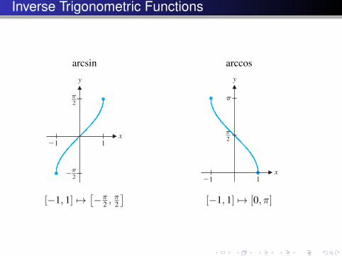
Inverse Trigonometric Functions
arcsin arccos
Mathematicians often use the notation arcsin x in place of sin−1 x . People will read sin−1 x inter-changeably as “inverse sine of x’’ or “arcsine of x.’’
Evaluate sin−1(√
32
).
Solution We look for the angle θ in the interval [−π
2 , π2
]for which sin θ =
√3
2 .
Note that since sin(
π3
) =√
32 and π
3 ∈ [−π2 , π
2
], we have that sin−1
(√3
2
) = π3 .
■
Evaluate sin−1(− 1
2
).
Solution Here, note that sin(−π
6
) = − 12 and −π
6 ∈ [−π2 , π
2
]. Thus,
sin−1
(−1
2
)= −π
6.
■
Judging by the preceding two examples, you might think that (7.1) is a roundaboutway of defining a function. If so, you’ve got the idea exactly. In fact, we want to emphasizethat what we know about the inverse sine function is principally through reference to thesine function. We will not have any other definition of arcsine, nor are there any algebraicformulas for this function. (These things are true of most inverse functions.) Further, youshould recall from our discussion in section 6.2 that we can draw a graph of y = sin−1 xsimply by reflecting the graph of y = sin x on the interval
[−π2 , π
2
](from Figure 6.34)
through the line y = x (see Figure 6.35).Turning to y = cos x, can you think of how to restrict the domain to make the function
one-to-one? Notice that restricting the domain to the interval [−π
2 , π2
], as we did for the
inverse sine function will not work here. (Why not?) The simplest way to do this is to re-strict its domain to the interval [0, π] (see Figure 6.36). Consequently, we define the in-verse cosine function by
(7.3)
Note that here, we have
cos(cos−1 x) = x, for all x ∈ [−1, 1]
and
cos−1(cos x) = x, for all x ∈ [0, π].
As with the definition of arcsine, it is helpful to think of cos−1 x as that angle θ in [0, π]for which cos θ = x . As with sin−1 x , it is common to use cos−1 x and arccos xinterchangeably.
y = cos−1 x if and only if cos y = x and 0 ≤ y ≤ π.
Evaluating an Inverse Sine with a Negative ArgumentExample 7.2
Evaluating an Inverse SineExample 7.1
Remark 7.1
Section 6.7 The Inverse Trigonometric Functions 531
y
x
�q
q
1�1
Figure 6.35
y = sin−1 x .
y
xq p
�1
1
Figure 6.36
y = cos x on [0, π].
smi98485_ch06b.qxd 5/17/01 1:36 PM Page 531
Evaluate cos−1(0).
Solution You will need to find that angle θ in [0, π] for which cos θ = 0. It’s nothard to see that cos−1(0) = π
2 . If you calculate this on your calculator and get 90,your calculator is in degrees mode. In this event, you should immediately change it toradians mode.
■
Evaluate cos−1(− √
22
).
Solution Here, look for the angle θ ∈ [0, π] for which cos θ = −√
22 . Notice that
cos(
3π4
) = −√
22 and 3π
4 ∈ [0, π] . Consequently,
cos−1
(−
√2
2
)= 3π
4.
■
Once again, we obtain the graph of this inverse function by reflecting the graphof y = cos x on the interval [0, π] (seen in Figure 6.36) through the line y = x (seeFigure 6.37).
We can define inverses for each of the four remaining trig functions in similar ways.For y = tan x, we restrict the domain to the interval
(−π2 , π
2
). Think about why the end-
points of this interval are not included (see Figure 6.38). Having done this, you shouldreadily see that we define the inverse tangent function by
(7.4)
The graph of y = tan−1 x is then as seen in Figure 6.39, found by reflecting the graph inFigure 6.38 through the line y = x .
y = tan−1 x if and only if tan y = x and − π2 < y < π
2 .
Evaluating an Inverse Cosine with a Negative ArgumentExample 7.4
Evaluating an Inverse CosineExample 7.3
532 Chapter 6 Exponentials, Logarithms and Other Transcendental Functions
q�q
�6
�4
�2
2
4
6
y
x
Figure 6.38
y = tan x on(−π
2 , π2
).
y
x
�q
q
4 62�6 �4 �2
Figure 6.39
y = tan−1 x .
y
x1�1
q
p
Figure 6.37
y = cos−1 x .
smi98485_ch06b.qxd 5/17/01 1:36 PM Page 532
[−1, 1] 7→[−π
2 ,π2
][−1, 1] 7→ [0, π]
Inverse Trigonometric Functions
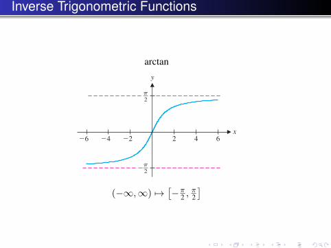
arctan
Evaluate cos−1(0).
Solution You will need to find that angle θ in [0, π] for which cos θ = 0. It’s nothard to see that cos−1(0) = π
2 . If you calculate this on your calculator and get 90,your calculator is in degrees mode. In this event, you should immediately change it toradians mode.
■
Evaluate cos−1(− √
22
).
Solution Here, look for the angle θ ∈ [0, π] for which cos θ = −√
22 . Notice that
cos(
3π4
) = −√
22 and 3π
4 ∈ [0, π] . Consequently,
cos−1
(−
√2
2
)= 3π
4.
■
Once again, we obtain the graph of this inverse function by reflecting the graphof y = cos x on the interval [0, π] (seen in Figure 6.36) through the line y = x (seeFigure 6.37).
We can define inverses for each of the four remaining trig functions in similar ways.For y = tan x, we restrict the domain to the interval
(−π2 , π
2
). Think about why the end-
points of this interval are not included (see Figure 6.38). Having done this, you shouldreadily see that we define the inverse tangent function by
(7.4)
The graph of y = tan−1 x is then as seen in Figure 6.39, found by reflecting the graph inFigure 6.38 through the line y = x .
y = tan−1 x if and only if tan y = x and − π2 < y < π
2 .
Evaluating an Inverse Cosine with a Negative ArgumentExample 7.4
Evaluating an Inverse CosineExample 7.3
532 Chapter 6 Exponentials, Logarithms and Other Transcendental Functions
q�q
�6
�4
�2
2
4
6
y
x
Figure 6.38
y = tan x on(−π
2 , π2
).
y
x
�q
q
4 62�6 �4 �2
Figure 6.39
y = tan−1 x .
y
x1�1
q
p
Figure 6.37
y = cos−1 x .
smi98485_ch06b.qxd 5/17/01 1:36 PM Page 532
(−∞,∞) 7→[−π
2 ,π2
]

Inverse Trigonometric Functions
arcsec
Evaluate tan−1(1).
Solution You must look for the angle, θ on the interval (−π
2 , π2
)for which
tan θ = 1. This is easy enough. Since tan(
π4
) = 1 and π4 ∈ (−π
2 , π2
), we have that
tan−1(1) = π4 .
■
We now turn to defining an inverse for sec x . First, we must issue a disclaimer. As wehave indicated, there are any number of ways to suitably restrict the domains of thetrigonometric functions in order to make them one-to-one. With the first three we’ve seen,there has been an obvious choice of how to do this and there is general agreement amongmathematicians on the choice of these intervals. In the case of sec x, this is not true. Thereare several reasonable ways in which to suitably restrict the domain and different authorsrestrict these differently. We have (arbitrarily) chosen to restrict the domain to be[0, π
2
) ∪ (π2 , π
]. You might initially think that this looks strange. Why not use all of [0, π]?
You need only think about the definition of sec x to see why we needed to exclude the pointx = π
2 . See Figure 6.40 for a graph of sec x on this domain. (Note the vertical asymptote atx = π
2 .) Consequently, we define the inverse secant function by
(7.5)
A graph of sec−1 x is shown in Figure 6.41.
Evaluate sec−1(−√2).
Solution You must look for the angle θ with θ ∈ [0, π
2
) ∪ (π2 , π
], for which
sec θ = −√2. Notice that if sec θ = −√
2, then cos θ = − 1√2
= −√
22 . Recall from
example 7.4 that cos 3π4 = −
√2
2 . Further, the angle 3π4 is in the interval
(π2 , π
]and so,
sec−1(−√2) = 3π
4 .
■
Calculators do not usually have built-in functions for sec x or sec−1 x . In this case, youmust convert the desired secant value to a cosine value and use the inverse cosine function,as we did in example 7.6.
We can likewise define inverses to cot x and csc x . As these functions are used only infrequently, wewill omit them here and examine them in the exercises.
Often, as a part of a larger problem (for example, evaluating an integral by some ofthe methods discussed in Chapter 7) you will need to recognize some relationship betweenthe trigonometric functions and their inverses. We present several clues here. When you arefaced with these problems, our best advice is to keep in mind the definitions of the inversefunctions and then draw a picture.
Remark 7.2
Evaluating an Inverse SecantExample 7.6
y = sec−1 x if and only if sec y = x and y ∈ [0, π
2
) ∪ (π2 , π
].
Evaluating an Inverse TangentExample 7.5
Section 6.7 The Inverse Trigonometric Functions 533
y
x
q
1051�5 �1�10
p
Figure 6.41
y = sec−1 x .
y
xp
�10
�5
�1
5
1
10
q
Figure 6.40
y = sec x on [0, π].
smi98485_ch06b.qxd 5/17/01 1:36 PM Page 533
(−∞,∞) 7→ [0, π]

Exponentials and Logarithmic Functions
DefinitionFor any constant b > 0, the function f (x) = bx is called anexponential function. Here, b is called the base and x is theexponent.
The most common exponential function, referred to as theexponential, is ex. This is the most common because of itsnice integral and differential properties.The number e is an irrational number defined by
e = limn→∞
(1 +
1n
)n
≈ 2.718281828459 . . . .
Algebraic properties of the exponential function
exey = ex+y
(ex)y = exy

Exponential and Logarithmic Function
DefinitionFor any positive number b 6= 1, the logarithm function with baseb, written logb x, is defined by
y = logb x ⇐⇒ x = by.
As with exponential functions, the most useful bases turnout to be 2, 10, and e.We usually abbreviate log10 x by log x.Similarly, loge x is usually abbreviated ln x (for naturallogarithm).The functions ex and ln x are inverse of each other
eln x = x for any x > 0,
and, by definition,
ln(ex) = x for any x.

Exponential and Logarithmic Function

Exponential and Logarithmic Function
TheoremFor any positive base b 6= 1 and positive numbers x and y,
(i) logb x is defined only for x > 0,(ii) logb 1 = 0,(iii) logb(xy) = logb x + logb y,(iv) logb(x/y) = logb x− logb y,(v) logb(x
y) = y logb x.
ExerciseWrite each as a single logarithm:(a) log2 27x − log2 3x
(b) ln 8− 3 ln(1/2)

Exponential and Logarithmic Function
Using the rules of exponents and logarithms, notice thatwe can rewrite any exponential as an exponential withbase e, as follows. For any base a > 0, we have
ax = eln(ax) = ex ln a.
Using these same properties we can rewrite any logarithmin terms of natural logarithms, as follows. For any positivebase b (b 6= 1), we have
logb x =ln xln b
.

Euler’s Formula
The relation between trigonometric and exponentialfunctions is given by the Euler’s formula
eix = cos x + i sin x.
The i in the exponent is the imaginary number i ≡√−1,
i.e. i2 = −1.In many engineering areas, the symbol i =
√−1 is often
replaced by j =√−1.
Imaginary numbers are part of complex numbers, C.Real numbers are also part of complex numbers.
Exercise1 Show that e−ix = cos x− i sin x.2 Use Euler’s formula to prove the following trigonometric
identities: (i) cos(x + y) = cos x cos y− sin x sin y, and(ii) sin(x + y) = sin x cos y + cos x sin y.

Exercise
Exercise1 Find the domain of
f (x) =1√
x2 − 3x + 2.
2 Find the domain of
f (x) = ln(x3 − 6x2 + 8x).

The Exponential
What is the exponential function ex?We know e0 = 1, but what is eπ? or ei?
Definition (The Exponential ex)The exponential function is defined using the following series(i.e. ‘long polynomial’)
ex = 1 + x +x2
2!+
x3
3!+
x4
4!+ · · ·
=
∞∑k=0
xk
k!
where k! ≡ k(k − 1)(k − 2) . . . 3 · 2 · 1, and 0! ≡ 1.
When x = 0 we get the expected result e0 = 1.Note that the true value of e = 1 + 1 + 1
2! +13! + · · · .

The Exponential
The exponential function has the following propertiesex+y = exey
exy = (ex)y
ddx ex = ex∫
ex dx = ex + C
Example
ddx
ex =ddx
(1 + x +
x2
2!+
x3
3!+
x4
4!+ · · ·
)= 0 + 1 +
2x2!
+3x2
3!+
4x3
4!· · ·
= 1 + x +x2
2!+
x3
3!+
x4
4!+ · · · = ex

Euler’s Formula
Recall the imaginary number i is defined by i ≡√−1.
So i2 = −1, i3 = −i, i4 = 1, and this continues cyclically.Recall the Euler’s Formula:
eix = cos x + i sin x,
and using the series definition of the exponential function
eix = 1 + ix +(ix)2
2!+
(ix)3
3!+
(ix)4
4!+ · · ·
= 1 + ix +i2x2
2!+
i3x3
3!+
i4x4
4!+ · · ·
= 1 + ix− x2
2!− i
x3
3!+
x4
4!+ i
x5
5!+ · · ·
=
(1− x2
2!+
x4
4!− · · ·
)︸ ︷︷ ︸
cos x
+i(
x− x3
3!+
x5
5!− · · ·
)︸ ︷︷ ︸
sin x
Euler’s Formula
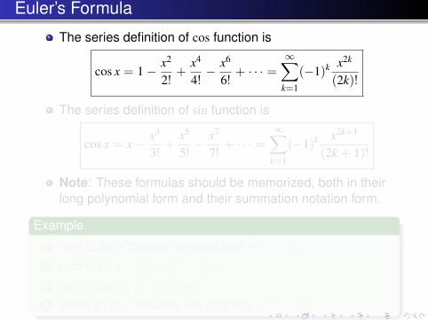
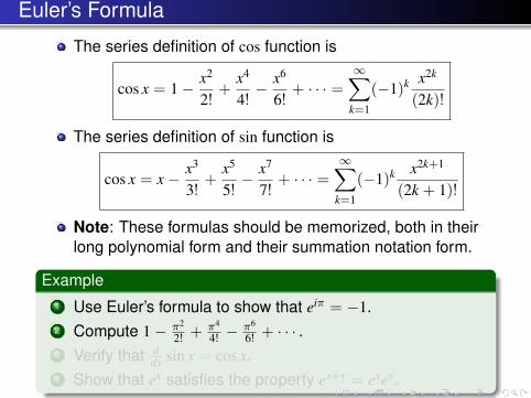
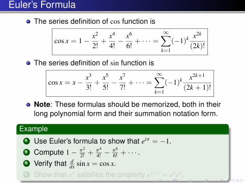
The series definition of cos function is
cos x = 1− x2
2!+
x4
4!− x6
6!+ · · · =
∞∑k=1
(−1)k x2k
(2k)!
The series definition of sin function is
cos x = x− x3
3!+
x5
5!− x7
7!+ · · · =
∞∑k=1
(−1)k x2k+1
(2k + 1)!
Note: These formulas should be memorized, both in theirlong polynomial form and their summation notation form.
Example1 Use Euler’s formula to show that eiπ = −1.2 Compute 1− π2
2! +π4
4! −π6
6! + · · · .3 Verify that d
dx sin x = cos x.4 Show that ex satisfies the property ex+y = exey.

Euler’s Formula
The series definition of cos function is
cos x = 1− x2
2!+
x4
4!− x6
6!+ · · · =
∞∑k=1
(−1)k x2k
(2k)!
The series definition of sin function is
cos x = x− x3
3!+
x5
5!− x7
7!+ · · · =
∞∑k=1
(−1)k x2k+1
(2k + 1)!
Note: These formulas should be memorized, both in theirlong polynomial form and their summation notation form.
Example1 Use Euler’s formula to show that eiπ = −1.2 Compute 1− π2
2! +π4
4! −π6
6! + · · · .3 Verify that d
dx sin x = cos x.4 Show that ex satisfies the property ex+y = exey.

Series definition of ex
f0(x) = 1
f1(x) = 1 + x
f2(x) = 1 + x + x2
2
f3(x) = 1 + x + x2
2 + x3
6...
Each polynomial in the sequence is, in a sense, the bestapproximation possible of that degree.The more terms included, the better the approximation.This is how calculators compute the exponential function(without having to add up infinitely many things).

Taylor Series
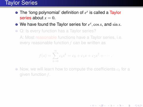
The ‘long polynomial’ definition of ex is called a Taylorseries about x = 0.We have found the Taylor series for ex, cos x, and sin x.Q: Is every function has a Taylor series?A: Most reasonable functions have a Taylor series, i.e.every reasonable function f can be written as
f (x) =∞∑
k=0
ckxk = c0 + c1x + c2x2 + · · · .
Now, we will learn how to compute the coefficients ck for agiven function f .
Taylor Series
The ‘long polynomial’ definition of ex is called a Taylorseries about x = 0.We have found the Taylor series for ex, cos x, and sin x.Q: Is every function has a Taylor series?A: Most reasonable functions have a Taylor series, i.e.every reasonable function f can be written as
f (x) =∞∑
k=0
ckxk = c0 + c1x + c2x2 + · · · .
Now, we will learn how to compute the coefficients ck for agiven function f .

Taylor Series
Definition (Taylor Series)Taylor series at x = 0 (also known as Maclaurin series) is
f (x) = f (0) +f ′(x)
1!x +
f ′′(0)2!
x2 +f ′′′(0)
3!x3 + · · · =
∞∑k=0
f (k)(0)k!
xk,
where f (k)(x) is the kth derivative of f evaluated at x = 0. Inother words, the coefficient ck is given by
ck =f (k)(0)
k!=
1k!
dkfdxk
∣∣∣∣0.
The definition only actually requires information about thefunction at a single point (in this case, 0).It is best to think of the Taylor series as a way of turning afunction into a long polynomial (series).

Taylor Series
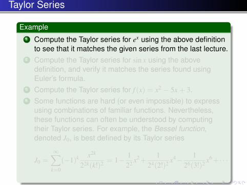
Example1 Compute the Taylor series for ex using the above definition
to see that it matches the given series from the last lecture.2 Compute the Taylor series for sin x using the above
definition, and verify it matches the series found usingEuler’s formula.
3 Compute the Taylor series for f (x) = x2 − 5x + 3.4 Some functions are hard (or even impossible) to express
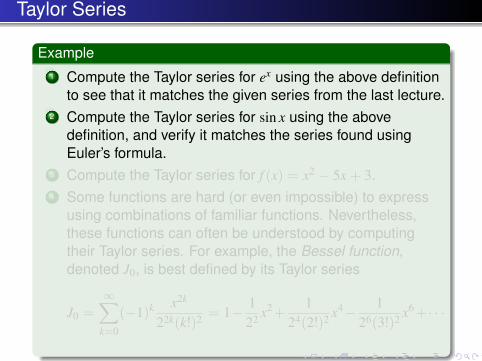
using combinations of familiar functions. Nevertheless,these functions can often be understood by computingtheir Taylor series. For example, the Bessel function,denoted J0, is best defined by its Taylor series
J0 =
∞∑k=0
(−1)k x2k
22k(k!)2 = 1− 122 x2+
124(2!)2 x4− 1
26(3!)2 x6+· · ·
Taylor Series
Example1 Compute the Taylor series for ex using the above definition
to see that it matches the given series from the last lecture.2 Compute the Taylor series for sin x using the above
definition, and verify it matches the series found usingEuler’s formula.
3 Compute the Taylor series for f (x) = x2 − 5x + 3.4 Some functions are hard (or even impossible) to express
using combinations of familiar functions. Nevertheless,these functions can often be understood by computingtheir Taylor series. For example, the Bessel function,denoted J0, is best defined by its Taylor series
J0 =
∞∑k=0
(−1)k x2k
22k(k!)2 = 1− 122 x2+
124(2!)2 x4− 1
26(3!)2 x6+· · ·
Taylor Series
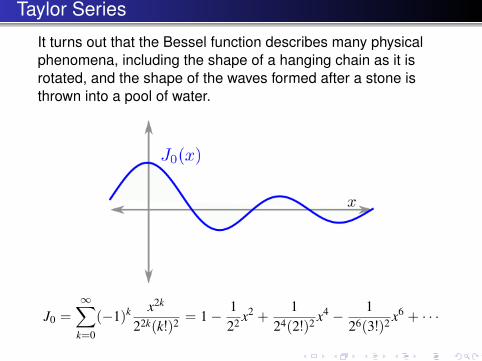
It turns out that the Bessel function describes many physicalphenomena, including the shape of a hanging chain as it isrotated, and the shape of the waves formed after a stone isthrown into a pool of water.
J0 =
∞∑k=0
(−1)k x2k
22k(k!)2 = 1− 122 x2 +
124(2!)2 x4 − 1
26(3!)2 x6 + · · ·

Taylor Series
Taylor series is useful because it turns a potentiallycomplicated function into something simple: a polynomial.Granted, this polynomial is infinitely long in general, but inpractice it is only necessary to compute the first few termsto get a good, local approximation of the function.The more terms one includes, the better the polynomialapproximates the function.
Particle with position p(t).At t = 0, the position is 5:
p0(t) = 5.At t = 0, the velocity is 3:
p1(t) = 5 + 3t.At t = 0, the acceleration is −4:
p2(t) = 5 + 3t − 2t2.
Taylor Series
Exercise1 Find the Taylor series for 1
x sin(x2) by substitution.2 Find the Taylor series for ex3
by substitution.3 Find the Taylor series for f (x) = cos2 x by combining terms.4 Use the trigonometric identity
cos2 x =1 + cos(2x)
2
and substitution to find the series for cos2 x. Try to give theseries in summation notation (other than the first term).

Hyperbolic Functions
DefinitionThe hyperbolic sine function is defined by
sinh x =ex − e−x
2
The hyperbolic cosine function is defined by
sinh x =ex + e−x
2
The hyperbolic tangent function is defined by
tanh x =sinh xcosh x
=ex − e−x
ex + e−x

Hyperbolic Functions
DefinitionThe hyperbolic sine function is defined by
sinh x =ex − e−x
2
The hyperbolic cosine function is defined by
sinh x =ex + e−x
2
The hyperbolic tangent function is defined by
tanh x =sinh xcosh x
=ex − e−x
ex + e−x

Hyperbolic Functions
DefinitionThe hyperbolic sine function is defined by
sinh x =ex − e−x
2
The hyperbolic cosine function is defined by
sinh x =ex + e−x
2
The hyperbolic tangent function is defined by
tanh x =sinh xcosh x
=ex − e−x
ex + e−x
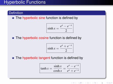
Hyperbolic Functions
DefinitionThe hyperbolic sine function is defined by
sinh x =ex − e−x
2
The hyperbolic cosine function is defined by
sinh x =ex + e−x
2
The hyperbolic tangent function is defined by
tanh x =sinh xcosh x
=ex − e−x
ex + e−x

Hyperbolic Functions
ExerciseVerify the following:(a) cosh2 u− sinh2 u = 1.(b) d
dx sinh x = cosh x.

Hyperbolic Functions
ExerciseVerify the following:(a) cosh2 u− sinh2 u = 1.(b) d
dx sinh x = cosh x.

Hyperbolic Functions
ExerciseVerify the following:(a) cosh2 u− sinh2 u = 1.(b) d
dx sinh x = cosh x.

Hyperbolic Functions
The hyperbolic cosine and hyperbolic sine give the x and ycoordinates, respectively, for points on the hyperbolax2 − y2 = 1.
[Compare this to the sine and cosine functions which give the xand y coordinates for points on the unit circle x2 + y2 = 1.]

Hyperbolic Functions
Example1 Using the Taylor series for ex and substitution, show that
the Taylor series for cosh and sinh are
cosh x = 1 +x2
2!+
x4
4!+ · · · =
∞∑k=0
x2k
(2k)!,
sinh x = x +x3
3!+
x5
5!+ · · · =
∞∑k=0
x2k+1
(2k + 1)!.

Hyperbolic Functions
Example (cont.)S: Using the Taylor series for ex and substitution
cosh x =ex + e−x
2
=12
[(1 + x +
x2
2!+ · · ·
)+
(1− x +
x2
2!− · · ·
)]=
12
[2 + 2
x2
2!+ 2
x4
4!+ · · ·
]= 1 +
x2
2!+
x4
4!+ · · ·
=
∞∑k=0
x2k
(2k)!

Hyperbolic Functions
Example (cont.)S: Using the Taylor series for ex and substitution
sinh x =ex − e−x
2
=12
[(1 + x +
x2
2!+ · · ·
)−(
1− x +x2
2!− · · ·
)]=
12
[2x + 2
x3
3!+ 2
x5
5!+ · · ·
]= x +
x3
3!+
x5
5!+ · · ·
=
∞∑k=0
x2k+1
(2k + 1)!

Hyperbolic Functions
Example2 By differentiating the Taylor series for sinh & cosh, show that
ddx
sinh x = cosh x,
ddx
cosh x = sinh x.

Hyperbolic Functions
Example (cont.)S: Differentiating hyperbolic sine gives
ddx
sinh x =ddx
∞∑k=0
x2k+1
(2k + 1)!=
∞∑k=0
(2k + 1)x2k
(2k + 1)!
=
∞∑k=0
x2k
(2k)!= cosh x
Differentiating hyperbolic cosine gives
ddx
cosh x =ddx
∞∑k=0
x2k
(2k)!=
∞∑k=0
(2k)x2k−1
(2k)!
=
∞∑k=1
x2k−1
(2k − 1)!=
∞∑k=0
x2k+1
(2k + 1)!= sinh x

Higher Order Terms in Taylor Series
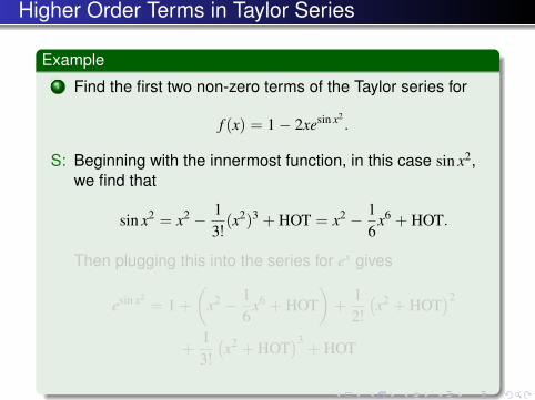
Example1 Find the first two non-zero terms of the Taylor series for
f (x) = 1− 2xesin x2.
S: Beginning with the innermost function, in this case sin x2,we find that
sin x2 = x2 − 13!(x2)3 + HOT = x2 − 1
6x6 + HOT.
Then plugging this into the series for ex gives
esin x2= 1 +
(x2 − 1
6x6 + HOT
)+
12!(x2 + HOT
)2
+13!(x2 + HOT
)3+ HOT

Higher Order Terms in Taylor Series
Example1 Find the first two non-zero terms of the Taylor series for
f (x) = 1− 2xesin x2.
S: Beginning with the innermost function, in this case sin x2,we find that
sin x2 = x2 − 13!(x2)3 + HOT = x2 − 1
6x6 + HOT.
Then plugging this into the series for ex gives
esin x2= 1 +
(x2 − 1
6x6 + HOT
)+
12!(x2 + HOT
)2
+13!(x2 + HOT
)3+ HOT

Higher Order Terms in Taylor Series
Example (cont.)Continuing from previous page
esin x2= . . . = 1 + x2 +
12
x4 +
(16− 1
6
)x6 + HOT
= 1 + x2 +12
x4 + HOT
Then to complete the answer, plug this into the originalfunction to find
f (x) = 1− 2x(
1 + x2 +12
x4 + HOT)
= 1− 2x− 2x3 − x5 + HOT

Higher Order Terms in Taylor Series
Example (cont.)Continuing from previous page
esin x2= . . . = 1 + x2 +
12
x4 +
(16− 1
6
)x6 + HOT
= 1 + x2 +12
x4 + HOT
Then to complete the answer, plug this into the originalfunction to find
f (x) = 1− 2x(
1 + x2 +12
x4 + HOT)
= 1− 2x− 2x3 − x5 + HOT

Higher Order Terms in Taylor Series
Example (cont.)Continuing from previous page
esin x2= . . . = 1 + x2 +
12
x4 +
(16− 1
6
)x6 + HOT
= 1 + x2 +12
x4 + HOT
Then to complete the answer, plug this into the originalfunction to find
f (x) = 1− 2x(
1 + x2 +12
x4 + HOT)
= 1− 2x− 2x3 − x5 + HOT

Higher Order Terms in Taylor Series
Example2 Compute the Taylor series (at 0) for sin2 x up to and
including terms of order 6. Try to give the full Taylor seriesin summation notation.
S: Using the Taylor series definition for sin x and substitution
sin2 x =
(x− x3
3!+
x5
5!− · · ·
)(x− x3
3!+
x5
5!− · · ·
)= x2 +
(−1
3− 1
3
)x4 +
(15!
+1
(3!)2 +15!
)x6 + · · ·
= x2 − 13
x4 +2
45x6 − · · · .

Higher Order Terms in Taylor Series
Example (cont.)S: To get the full Taylor series, one can use the identity
sin2 x =1− cos(2x)
2
to find that
sin2 x =1− cos(2x)
2=
12
(1−
(1− (2x)2
2!+
(2x)4
4!− · · ·
))=
12
((2x)2
2!+
(2x)4
4!− (2x)6
6!+ · · ·
)=
12
∞∑k=1
(−1)k−1 (2x)2k
(2k)!

Higher Order Terms in Taylor Series
Example (cont.)S: To get the full Taylor series, one can use the identity
sin2 x =1− cos(2x)
2
to find that
sin2 x =1− cos(2x)
2=
12
(1−
(1− (2x)2
2!+
(2x)4
4!− · · ·
))=
12
((2x)2
2!+
(2x)4
4!− (2x)6
6!+ · · ·
)=
12
∞∑k=1
(−1)k−1 (2x)2k
(2k)!

Convergence
There are two main issues of Taylor series expansion:1 A function may not have a Taylor series at all;2 A function’s Taylor series may not converge everywhere,
even within the function’s domain.
1 Functions without a Taylor seriesSome functions cannot be expressed in the form
f (x) =∞∑
k=0
ckxk = c0 + c1x + c2x2 + · · ·
Examples: tan which has vertical asymptotes, and ln whichis not defined for x ≤ 0. Polynomials are not able to capturethese sorts of discontinuities and asymptotes.
2 Taylor series might be well behaved for some values of xand non-nonsensical for other values of x.
Example: Geometric series
1 + x + x2 + x3 + x4 + · · · = 11− x
only holds when |x| < 1.
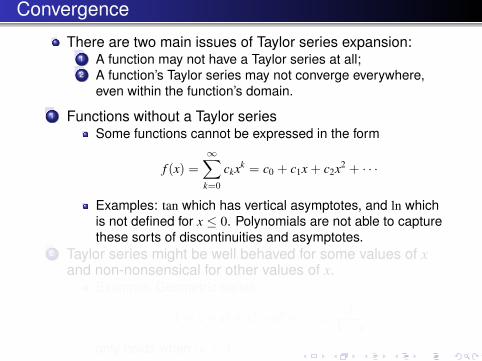

Convergence
Every Taylor series has a convergence domain, calledinterval of convergence, where the series is well-behaved,and outside that domain the series will not converge.For many functions, the domain is the whole real numberline (e.g. the series for ex, sin x, cos x, sinh x, and cosh x allconverge everywhere).

Convergence
ExampleA beam of light of intensity L hits a
pane of glass. Half of the light isreflected, and a third of the light istransmitted; the rest is absorbed.When a beam of light of intensity L
hits two parallel panes with an air gapbetween them, how much light istransmitted through both panes? (Thefollowing figure shows how the lightgets reflected and rereflected. Thefirst transmitted and reflected beamsof light are labeled with theirrespective intensities. The questionasks for the total of the beams of lightemerging on the right side of the rightpane of glass).

Convergence
Example (cont.)
Note that each beam is 14 the previous
beam. Thus the total light emerging on theright side of the right pane of glass is
L9+
L36
+L
144+ · · ·
=L9
(1 +
14+
116
+ · · ·)
=L9
(1
1− 14
)
=L9
43=
4L27,
by using the geometric series formula.

Taylor Series
Example
Use the Taylor series of 11−x to derive the Taylor series of ln(1 + x).
Hint: recall thatln(1 + x) =
∫1
1 + xdx.
S: Note that1
1 + x=
11− (−x)
= 1− x + x2 − x3 + x4 − · · ·
Integrating both sides∫dx
1 + x=
∫(1− x + x2 − x3 + x4 − · · · ) dx
⇔ ln(1 + x) + C = x− x2
2+
x3
3− · · · =
∞∑k=1
(−1)k−1 xk
k
Plugging x = 0 shows that C = 0, and so
ln(1 + x) = x− x2
2+
x3
3− · · · =
∞∑k=1
(−1)k−1 xk
k

Taylor Series
Example
Use the fact thatarctan x =
∫dx
1 + x2
to find the Taylor series for arctan x.S: Using the fact, and the geometric series,
arctan x =
∫1
1 + x2 dx =
∫1
1− (−x2)dx
=
∫(1− x2 + x4 − x6 + · · · ) dx, (|x| < 1)
= x− x3
3+
x5
5− x7
7+ · · ·+ C.
Plugging in x = 0 gives C = 0, since arctan 0 = 0. Thus,
arctan x = x− x3
3+
x5
5− · · · =
∞∑k=0
(−1)k x2k+1
2k + 1, (|x| < 1).
! arctan x is defined for all x, but its Taylor series only converges for |x| < 1.
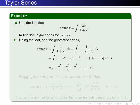

Taylor Series
ExerciseAnother important function is the binomial series (1 + x)α, where α issome constant. Show that
(1 + x)α = 1 + αx +α(α− 1)
2!x2 +
α(α− 1)(α− 2)3!
x3 + · · ·
=∞∑
k=0
(αk
)xk
where (αk
)=α(α− 1)(α− 2) · · · (α− k + 1)
k!.
! The series also only holds for |x| < 1.

Taylor Series
ExerciseAnother important function is the binomial series (1 + x)α, where α issome constant. Show that
(1 + x)α = 1 + αx +α(α− 1)
2!x2 +
α(α− 1)(α− 2)3!
x3 + · · ·
=∞∑
k=0
(αk
)xk
where (αk
)=α(α− 1)(α− 2) · · · (α− k + 1)
k!.
! The series also only holds for |x| < 1.

Taylor Series
ExerciseAnother important function is the binomial series (1 + x)α, where α issome constant. Show that
(1 + x)α = 1 + αx +α(α− 1)
2!x2 +
α(α− 1)(α− 2)3!
x3 + · · ·
=∞∑
k=0
(αk
)xk
where (αk
)=α(α− 1)(α− 2) · · · (α− k + 1)
k!.
! The series also only holds for |x| < 1.

Taylor Series: Summary
The following hold for all x:
ex =
∞∑k=0
xk
k!
cos x =
∞∑k=0
(−1)k x2k
(2k)!
sin x =
∞∑k=0
(−1)k x2k+1
(2k + 1)!
cosh x =
∞∑k=0
x2k
(2k)!
sinh x =
∞∑k=0
x2k+1
(2k + 1)!
The following hold for |x| < 1:
11− x
=
∞∑k=0
xk
ln(1 + x) =∞∑
k=1
(−1)k+1 xk
k
arctan x =
∞∑k=0
(−1)k x2k+1
2k + 1
(1 + x)α =
∞∑k=0
(αk
)xk


![Lambda Calculus - SJTUbasics.sjtu.edu.cn/~yuxi/teaching/lectures/Lambda Calculus.pdf · Logic as a variable free presentation of functions [1924]. von Neumann [28Dec.1903-8Feb.1957]](https://static.fdocuments.net/doc/165x107/5f613dccd32eec4b7917faeb/lambda-calculus-yuxiteachinglectureslambda-calculuspdf-logic-as-a-variable.jpg)

