Calculus of Variations & Variational Methods Unconstrained Minimization In preparation for an...
43
292 The calculus of variations is used to obtain extrema of expressions involving unknown functions called functionals. Applications range from simple geometric problems to finite-element methods to optimization theory. References : Ewing, G. M., Calculus of Variations with Applications, Dover, 1985. Hildebrand, F. B., Methods of Applied Mathematics, 2 nd Ed., Dover, 1992. Reddy & Rasmussen, Advanced Engineering Analysis, Kreiger 1990. Weinstock, R., Calculus of Variations with Applications to Physics and Engineering, Dover. Calculus of Variations & Variational Methods
Transcript of Calculus of Variations & Variational Methods Unconstrained Minimization In preparation for an...

292
The calculus of variations is used to obtain extrema of expressions involving unknown functions called functionals. Applications range from simple geometric problems to finite-element methods to optimization theory.References:
Ewing, G. M., Calculus of Variations with Applications, Dover, 1985.Hildebrand, F. B., Methods of Applied Mathematics, 2nd Ed., Dover, 1992.Reddy & Rasmussen, Advanced Engineering Analysis, Kreiger 1990.Weinstock, R., Calculus of Variations with Applications to Physics and Engineering, Dover.
Calculus of Variations & Variational Methods

293
Unconstrained MinimizationIn preparation for an introduction to the calculus of variations, recall maxima, minima (extrema), and inflections of functions from the differential calculus.
Calculus of Variations & Variational Methods
( )f x
maxf
0x
0dfdx
=
0
max 0
critical (stationary) point
( )critical value
x
f f x
=
==
( )f x
maxf
0x
0dfdx
=
( )f x
0x
0dfdx
=
local minimum
local maximum
inflection
294
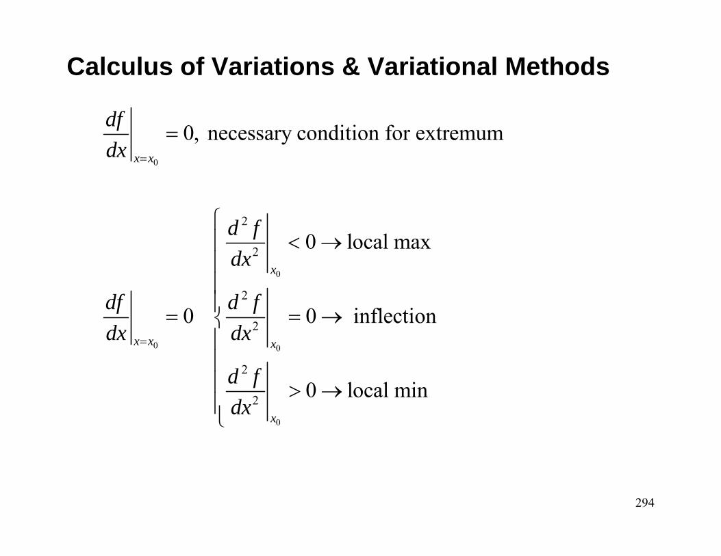
Calculus of Variations & Variational Methods
0
0, necessary condition for extremumx x
dfdx =
=
0
0 0
0
2
2
2
2
2
2
0 local max
0 0 inflection
0 local min
x
x x x
x
d fdx
df d fdx dx
d fdx
=
⎧< →⎪
⎪⎪⎪= = →⎨⎪⎪⎪ > →⎪⎩
295
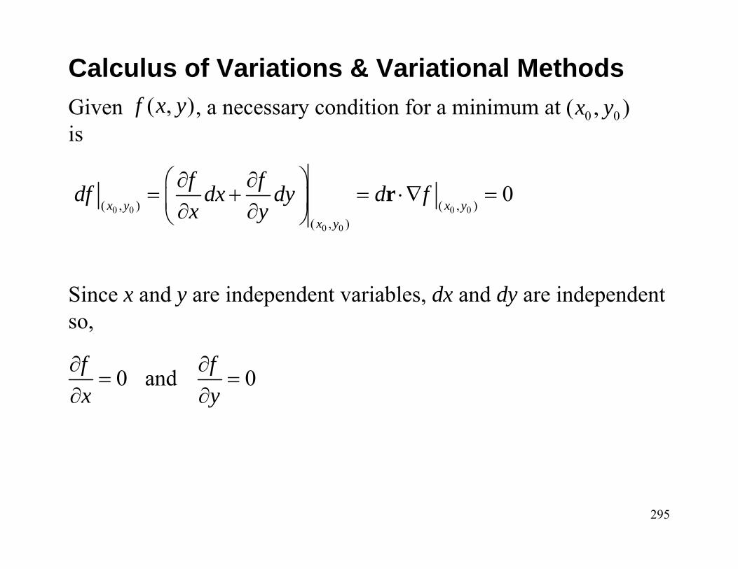
Given , a necessary condition for a minimum at is
Since x and y are independent variables, dx and dy are independent so,
Calculus of Variations & Variational Methods( , )f x y 0 0( , )x y
0 0 0 0
0 0
( , ) ( , )( , )
0x y x y
x y
f fdf dx dy d fx y
⎛ ⎞∂ ∂= + = ⋅∇ =⎜ ⎟∂ ∂⎝ ⎠
r
0 and 0f fx y∂ ∂
= =∂ ∂

296
Constrained MinimizationNow minimize f with a constraint, e.g.,
(1)Lagrange Multiplier MethodFrom (1),
We introduce the modified function with no constraints(2)
and set(3)
Calculus of Variations & Variational Methods
( , ) 0G x y =
0G Gdx dy d Gx y
∂ ∂+ = ⋅∇ =
∂ ∂r
( , , ) ( , ) ( , )LF x y f x y G x yλ λ≡ +
0L L LL
F F FdF dx dy dx y
λλ
∂ ∂ ∂= + + =
∂ ∂ ∂
297
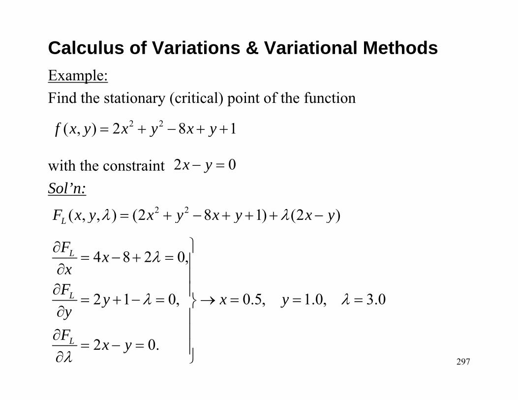
Example:Find the stationary (critical) point of the function
with the constraint Sol’n:
Calculus of Variations & Variational Methods
2 2( , ) 2 8 1f x y x y x y= + − + +
2 0x y− =
2 2( , , ) (2 8 1) (2 )LF x y x y x y x yλ λ= + − + + + −
4 8 2 0,
2 1 0, 0.5, 1.0, 3.0
2 0.
L
L
L
F xx
F y x yy
F x y
λ
λ λ
λ
⎫∂= − + = ⎪∂ ⎪
∂ ⎪= + − = → = = =⎬∂ ⎪⎪∂
= − = ⎪∂ ⎭
298
Calculus of Variations: Functionals and Euler EquationsThe focus of the calculus of variations is the determination of maxima and minima of expressions that involve unknown functions. Here we look at a few classical problems to introducesome of the concepts.
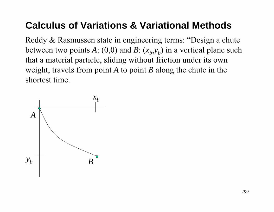
The Brachistochrone (the one that started it all):Weinstock gives the problem as it was originally stated by John Bernoulli in 1696: “Given two points A and B in a vertical plane, to find for the moveable particle M, the path AMB, descending along which by its own gravity, the beginning to be urged from point A, it may in the shortest time reach the point B.”
Calculus of Variations & Variational Methods
299
Reddy & Rasmussen state in engineering terms: “Design a chute between two points A: (0,0) and B: (xb,yb) in a vertical plane such that a material particle, sliding without friction under its ownweight, travels from point A to point B along the chute in the shortest time.
Calculus of Variations & Variational Methods
A
Byb
xb
300
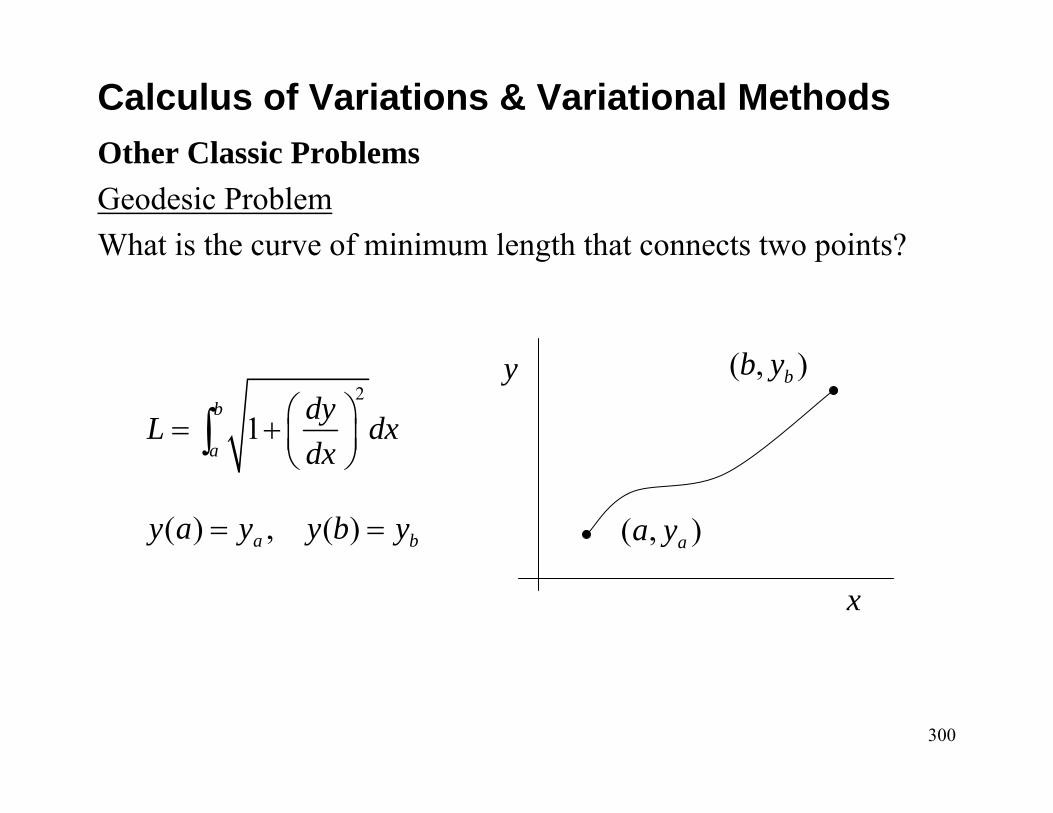
Other Classic ProblemsGeodesic ProblemWhat is the curve of minimum length that connects two points?
Calculus of Variations & Variational Methods
( ) , ( )a by a y y b y= = ( , )aa y
( , )bb y2
1b
a
dyL dxdx
⎛ ⎞= + ⎜ ⎟⎝ ⎠∫
x
y
301
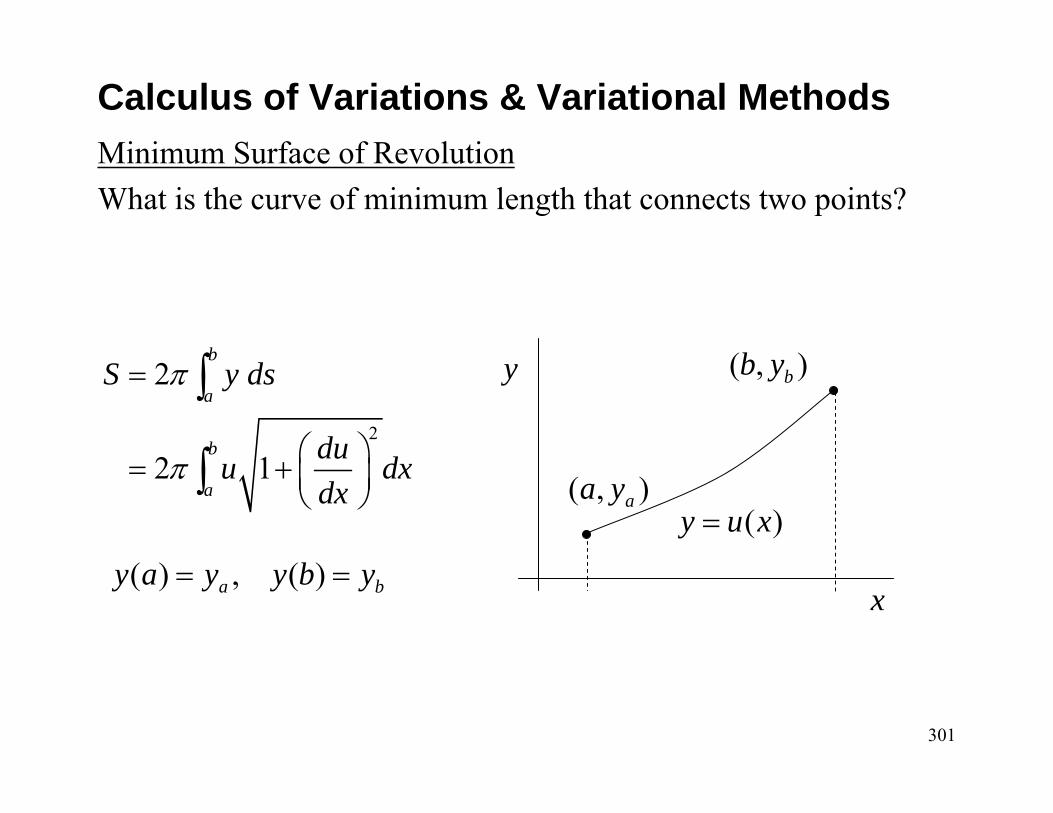
Minimum Surface of RevolutionWhat is the curve of minimum length that connects two points?
Calculus of Variations & Variational Methods
( , )aa y
( , )bb y
2
2
2 1
b
a
b
a
S y ds
duu dxdx
π
π
=
⎛ ⎞= + ⎜ ⎟⎝ ⎠
∫
∫
x
y
( )y u x=
( ) , ( )a by a y y b y= =
302
The Euler EquationEach of these problems presents the problem of finding a continuously differentiable function u(x) that minimizes the integral of the form
(1)And that satisfies the end conditions
We now suppose that u(x) is the minimizing function, then choose any continuously differentiable function η(x) and create a one-parameter ‘trial’ function
Calculus of Variations & Variational Methods
( ) ( , , )b
aI u F x u u dx′= ∫
( ) , ( )a bu a u u b u= =
( ) ( ) ( )y u x u x xαη= = +
303
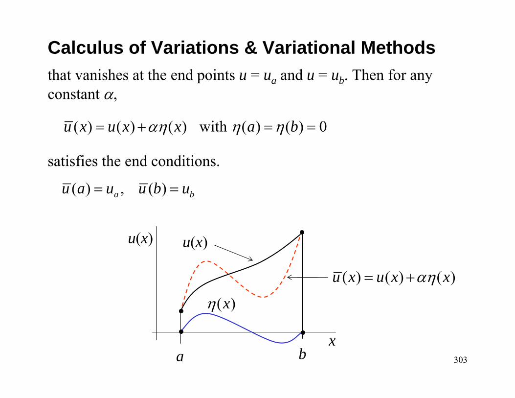
that vanishes at the end points u = ua and u = ub. Then for any constant α,
satisfies the end conditions.
Calculus of Variations & Variational Methods
( ) , ( )a bu a u u b u= =
( ) ( ) ( ) with ( ) ( ) 0u x u x x a bαη η η= + = =
( )xη
( ) ( ) ( )u x u x xαη= +
a bx
u(x) u(x)
304
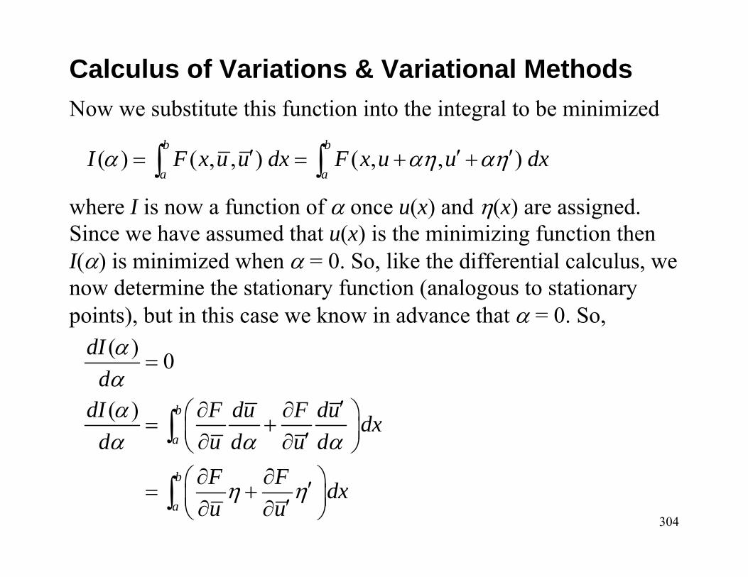
Now we substitute this function into the integral to be minimized
where I is now a function of α once u(x) and η(x) are assigned. Since we have assumed that u(x) is the minimizing function then I(α) is minimized when α = 0. So, like the differential calculus, we now determine the stationary function (analogous to stationary points), but in this case we know in advance that α = 0. So,
Calculus of Variations & Variational Methods
( ) ( , , ) ( , , )b b
a aI F x u u dx F x u u dxα αη αη′ ′ ′= = + +∫ ∫
( ) 0
( ) b
a
b
a
dId
dI F du F du dxd u d u d
F F dxu u
αααα α α
η η
=
′∂ ∂⎛ ⎞= +⎜ ⎟′∂ ∂⎝ ⎠∂ ∂⎛ ⎞′= +⎜ ⎟′∂ ∂⎝ ⎠
∫
∫
305
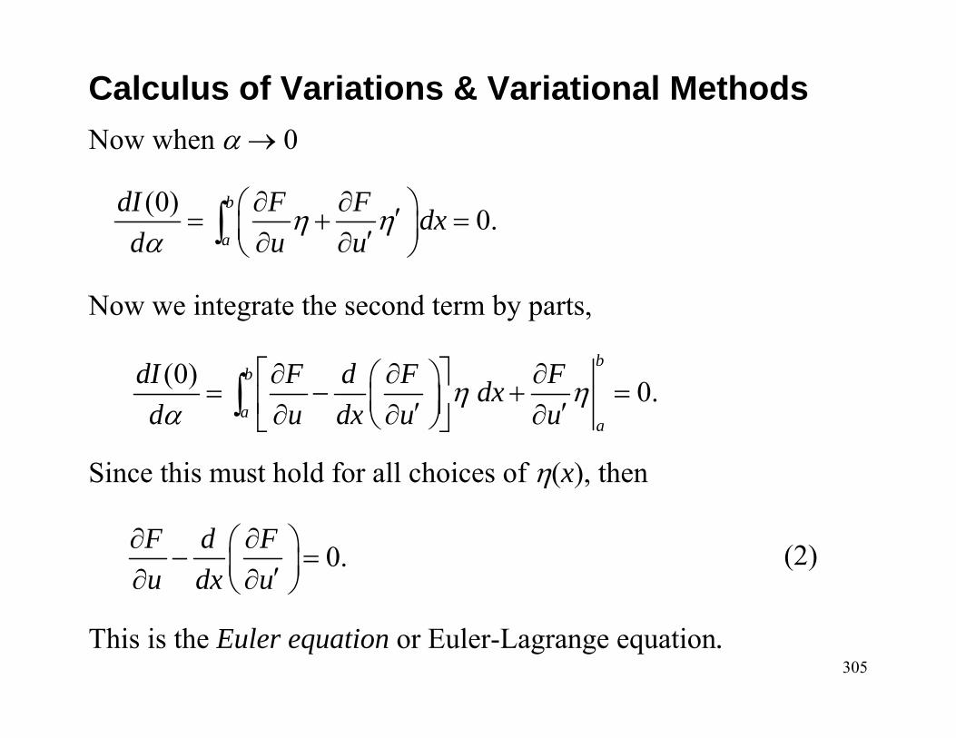
Now when α → 0
Now we integrate the second term by parts,
Since this must hold for all choices of η(x), then
(2)
This is the Euler equation or Euler-Lagrange equation.
Calculus of Variations & Variational Methods
(0) 0.b
a
dI F F dxd u u
η ηα
∂ ∂⎛ ⎞′= + =⎜ ⎟′∂ ∂⎝ ⎠∫
(0) 0.b
b
aa
dI F d F Fdxd u dx u u
η ηα
⎡ ⎤∂ ∂ ∂⎛ ⎞= − + =⎜ ⎟⎢ ⎥′ ′∂ ∂ ∂⎝ ⎠⎣ ⎦∫
0.F d Fu dx u
∂ ∂⎛ ⎞− =⎜ ⎟′∂ ∂⎝ ⎠

306
So, if u(x) minimizes I(u), it must satisfy the Euler equation. Solutions of the Euler equation are called extremals of the problem and an extremal that satisfies the end conditions is called a stationary function.
First IntegralsEquation (2) is written with partial derivatives that treat x, u, and u′as independent variables. The second term can be expanded to give
So, Eq. (2) is equivalent to
Calculus of Variations & Variational Methods
F F du F dux u u u dx u u dx
′∂ ∂ ∂ ∂ ∂ ∂⎛ ⎞ ⎛ ⎞ ⎛ ⎞+ +⎜ ⎟ ⎜ ⎟ ⎜ ⎟′ ′ ′ ′∂ ∂ ∂ ∂ ∂ ∂⎝ ⎠ ⎝ ⎠ ⎝ ⎠

307
(3)
This is a second-order ODE, unless so in general there are two arbitrary constants to satisfy the end conditions. One can show that (3) is also equivalent to
So, if F does not involve x explicitly,
This is a first integral of Euler’s equation.
Calculus of Variations & Variational Methods
if 0.F FF u Cu x∂ ∂′− = ≡′∂ ∂
2 2/ 0,F u′∂ ∂ ≡
1 0.d F du FFu dx u dx x⎡ ⎤∂ ∂⎛ ⎞− − =⎜ ⎟⎢ ⎥′ ′∂ ∂⎝ ⎠⎣ ⎦
2
2 ( ) 0.u u u u u x ud u duF F F Fdx dx′ ′ ′ ′+ + − =
308
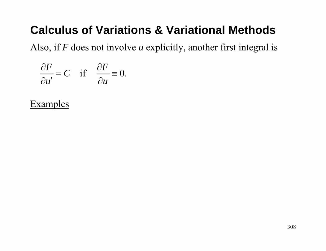
Also, if F does not involve u explicitly, another first integral is
Examples
Calculus of Variations & Variational Methods
if 0.F FCu u∂ ∂
= ≡′∂ ∂

309
Variational NotationThe notation of the calculus of variations shows many similarities to the differential calculus. Beginning with the integrand of the functional I(u)
We substituted for
with the trial function
Calculus of Variations & Variational Methods
( , , )F F x u u′=
( )y u x=
where is defined as the first variation of u(x).
( ) ( ) ( )( )
y u x u x xu x u
αηδ
= = += +
( )u xδ αη=
310
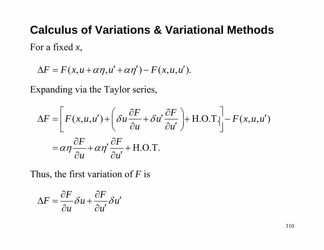
For a fixed x,
Expanding via the Taylor series,
Thus, the first variation of F is
Calculus of Variations & Variational Methods
( , , ) ( , , ).F F x u u F x u uαη αη′ ′ ′∆ = + + −
( , , ) H.O.T. ( , , )
H.O.T.
F FF F x u u u u F x u uu u
F Fu u
δ δ
αη αη
⎡ ⎤∂ ∂⎛ ⎞′ ′ ′∆ = + + + −⎜ ⎟⎢ ⎥′∂ ∂⎝ ⎠⎣ ⎦∂ ∂′= + +
′∂ ∂
F FF u uu uδ δ∂ ∂ ′∆ = +
′∂ ∂

311
This is analogous to the total differential,
Graphically,
Calculus of Variations & Variational Methods
F F FdF dx du dux u u
∂ ∂ ∂ ′= + +′∂ ∂ ∂
du
dx
( )xη
( ) ( ) ( )u x u x xαη= +
u u uδ = −
x fixed
du = the first-order approximation of the change along u(x) corresponding to a change in x of dx
δu = the first-order approximation to the changeto u at a fixed xu

312
Variational laws are analogous to differentiation,
The variation and derivative are commutative operators, i.e.,
This will be a very important result for us later.
Applying the notation to the functional
Calculus of Variations & Variational Methods
1 2 1 2 2 1
1 2 1 1 22
2 2
( ) ,
.
F F F F F F
F F F F FF F
δ δ δ
δ δδ
= +
⎛ ⎞ −=⎜ ⎟
⎝ ⎠
( )d duudx dx
δ δ ⎛ ⎞= ⎜ ⎟⎝ ⎠
( ) ( , , ) ,b
aI u F x u u dx′= ∫

313
Then
Integrating the second term by parts,
Then,
Calculus of Variations & Variational Methods
0.b
a
F F dI u u dxu u dx
δ δ δ∂ ∂⎡ ⎤= + =⎢ ⎥′∂ ∂⎣ ⎦∫
.b
b b
a aa
F d F d Fu dx u u dxu dx u dx u
δ δ δ∂ ∂ ∂⎛ ⎞= − ⎜ ⎟′ ′ ′∂ ∂ ∂⎝ ⎠∫ ∫
0
0
bb
aa
b
a
F d F FI u dx uu dx u u
F d FI u dxu dx u
δ δ δ
δ δ
⎡ ⎤∂ ∂ ∂⎛ ⎞= − + =⎜ ⎟⎢ ⎥′ ′∂ ∂ ∂⎝ ⎠⎣ ⎦
⎡ ⎤∂ ∂⎛ ⎞= − =⎜ ⎟⎢ ⎥′∂ ∂⎝ ⎠⎣ ⎦
∫
∫δu = 0 at end points

314
So,
Thus, we have recovered the Euler-Lagrange equation using the variational notation.
End ConditionsWe now look at the end conditions (more generally, boundary conditions). Start with
Applying Liebniz’s rule,
Calculus of Variations & Variational Methods
0.F d Fu dx u
∂ ∂⎛ ⎞− =⎜ ⎟′∂ ∂⎝ ⎠
( , , )b
aI F x u u dxδ δ ′= ∫

315
Integrating by parts,
Calculus of Variations & Variational Methods
[ ] [ ] (fixed end points)
= .
b
b aa
b
a
I F dx F b F a
F Fu u dxu u
δ δ δ δ
δ δ
= + −
∂ ∂⎡ ⎤′−⎢ ⎥′∂ ∂⎣ ⎦
∫
∫
0 0
=
( ) ( )
bb
aa
b
b aab a
F d F FI u dx uu dx u u
F d F F Fu dx u uu dx u u u
δ δ δ
δ δ δ
⎡ ⎤∂ ∂ ∂⎛ ⎞ ⎡ ⎤− +⎜ ⎟⎢ ⎥ ⎢ ⎥′ ′∂ ∂ ∂⎝ ⎠ ⎣ ⎦⎣ ⎦⎡ ⎤∂ ∂ ∂ ∂⎛ ⎞ ⎛ ⎞ ⎛ ⎞= − + −⎜ ⎟ ⎜ ⎟ ⎜ ⎟⎢ ⎥′ ′ ′∂ ∂ ∂ ∂⎝ ⎠ ⎝ ⎠ ⎝ ⎠⎣ ⎦
∫
∫
316
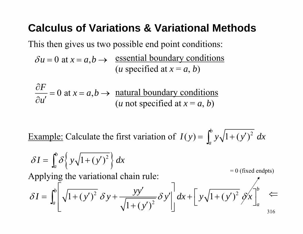
This then gives us two possible end point conditions:
Example: Calculate the first variation of
Applying the variational chain rule:
Calculus of Variations & Variational Methods
0 at ,
0 at ,
u x a b
F x a bu
δ = = →
∂= = →′∂
essential boundary conditions(u specified at x = a, b)
natural boundary conditions(u not specified at x = a, b)
2( ) 1 ( )b
aI y y y dx′= +∫
{ }21 ( )b
aI y y dxδ δ ′= +∫
2 2
21 ( ) 1 ( )
1 ( )
bb
a a
yyI y y y dx y y xy
δ δ δ δ⎡ ⎤′ ⎡ ⎤′ ′ ′= + + + +⎢ ⎥ ⎣ ⎦′+⎢ ⎥⎣ ⎦
∫
= 0 (fixed endpts)
⇐
317
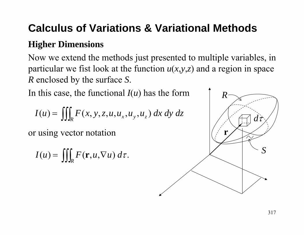
Higher DimensionsNow we extend the methods just presented to multiple variables, in particular we fist look at the function u(x,y,z) and a region in space R enclosed by the surface S.In this case, the functional I(u) has the form
or using vector notation
Calculus of Variations & Variational Methods
( ) ( , , , , , , )x y zRI u F x y z u u u u dx dy dz= ∫∫∫
( ) ( , , ) .R
I u F u u dτ= ∇∫∫∫ r
r
S
R
dτ
318
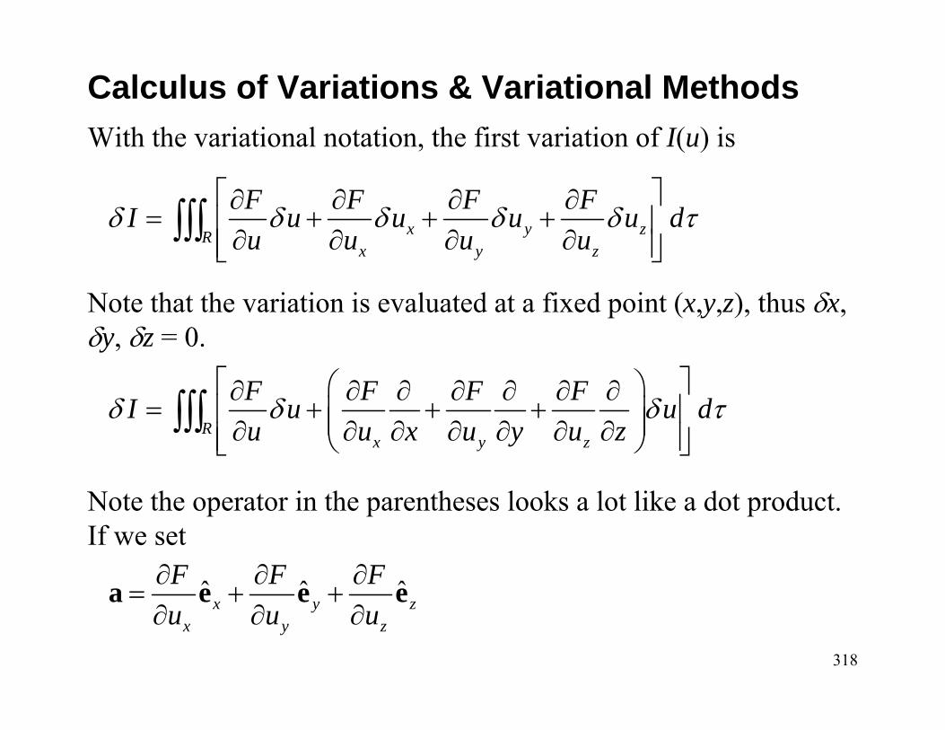
With the variational notation, the first variation of I(u) is
Note that the variation is evaluated at a fixed point (x,y,z), thus δx, δy, δz = 0.
Note the operator in the parentheses looks a lot like a dot product. If we set
Calculus of Variations & Variational Methods
x y zRx y z
F F F FI u u u u du u u u
δ δ δ δ δ τ⎡ ⎤∂ ∂ ∂ ∂
= + + +⎢ ⎥∂ ∂ ∂ ∂⎢ ⎥⎣ ⎦
∫∫∫
Rx y z
F F F FI u u du u x u y u z
δ δ δ τ⎡ ⎤⎛ ⎞∂ ∂ ∂ ∂ ∂ ∂ ∂
= + + +⎢ ⎥⎜ ⎟⎜ ⎟∂ ∂ ∂ ∂ ∂ ∂ ∂⎢ ⎥⎝ ⎠⎣ ⎦∫∫∫
ˆ ˆ ˆx y zx y z
F F Fu u u∂ ∂ ∂
= + +∂ ∂ ∂
a e e e

319
Then
For integration by parts, recall
So,
Calculus of Variations & Variational Methods
( ) .R
FI u u du
δ δ δ τ∂⎡ ⎤= + ⋅∇⎢ ⎥∂⎣ ⎦∫∫∫ a
( )( )
φ φ φφ φ φ
∇⋅ = ∇ ⋅ +∇ ⋅⋅∇ = ∇ ⋅ − ∇ ⋅
a a aa a a
( ) .R R
FI u d u du
δ δ τ δ τ∂⎡ ⎤= −∇ ⋅ + ∇ ⋅⎢ ⎥∂⎣ ⎦∫∫∫ ∫∫∫a a

320
Now use the divergence theorem on the last integral
Again, the necessary condition for minimizing I(u) is that δI = 0. Thus, the integrand of the volume integral must be zero, i.e.,
or
Calculus of Variations & Variational Methods
ˆ( ) .R S
FI u d u dSu
δ δ τ δ∂⎡ ⎤= −∇ ⋅ + ⋅⎢ ⎥∂⎣ ⎦∫∫∫ ∫∫a n a
0Fu
∂−∇ ⋅ =
∂a
0.x y z
F F F Fu x u y u z u
⎛ ⎞⎛ ⎞ ⎛ ⎞∂ ∂ ∂ ∂ ∂ ∂ ∂− − − =⎜ ⎟⎜ ⎟ ⎜ ⎟⎜ ⎟∂ ∂ ∂ ∂ ∂ ∂ ∂⎝ ⎠⎝ ⎠ ⎝ ⎠

321
This is the 3D Euler-Lagrange equation. The surface integral must also vanish, this gives three possible boundary conditions
i.)
ii.)
iii.)
Calculus of Variations & Variational Methods
specified on 0 on (essential)u S u Sδ→ =
ˆ + + 0 on (natural)x y zx y z
F F Fn n n Su u u∂ ∂ ∂
⋅ = =∂ ∂ ∂
n a
0 on part of (mixed)
ˆ on remainder of u S
Sδ = ⎫
⎬⋅ = ⎭n a
322
Note the steps used to obtain the Euler equation and the associated boundary conditions:
1. Take the first variation δI(u)
2. Use integration by parts to factor δu in the integrand
3. Use the divergence theorem to create a surface integral containing the boundary conditions
Calculus of Variations & Variational Methods
323
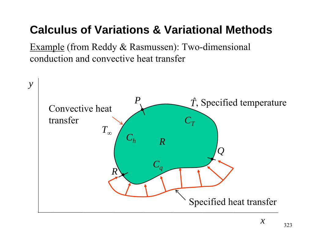
Example (from Reddy & Rasmussen): Two-dimensional conduction and convective heat transfer
Calculus of Variations & Variational Methods
T̂P
Q
R
R
Convective heat transfer
Specified heat transfer
, Specified temperature
T∞
x
y
Cq
CT
Ch
324
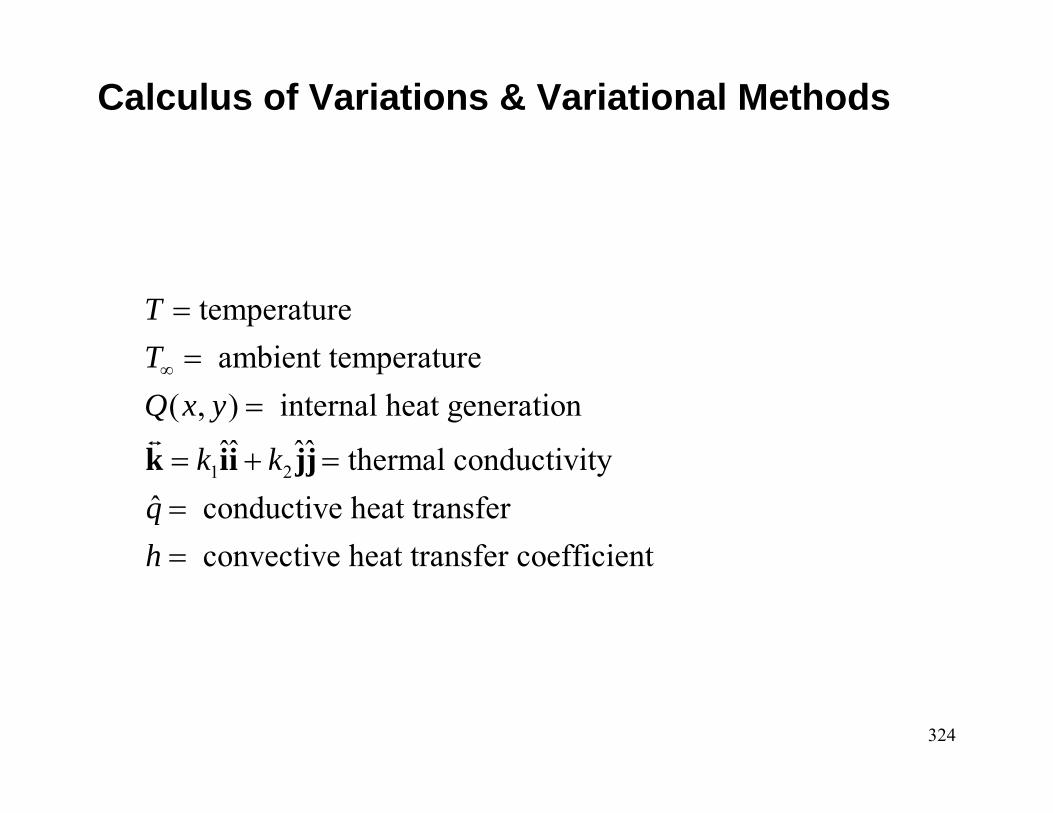
Calculus of Variations & Variational Methods
1 2
temperature ambient temperature
( , ) internal heat generationˆˆ ˆˆ thermal conductivity
ˆ conductive heat transfer convective heat transfer coefficient
TTQ x y
k kqh
∞
==
=
= + ===
k ii jj

325
Calculus of Variations & Variational Methods
Note that in this problem, we already have explicit boundary integrals. As before the interior integral (over R) will also generate a boundary integral after it is integrated by parts.
{ }
{ }
1 12 2
1 12 2
Minimize:
( ) ( )ˆ
First variation:
( ) ( ) ( )ˆ
q h
q h
R C C
R C C
I T T T QT dx dy qT ds h T T T ds
I T T T Q T dx dy q T ds h T T T dsδ δ δ δ δ
∞
∞
= ∇ ⋅ ⋅∇ + − + −⎡ ⎤⎣ ⎦
= ∇ ⋅ ⋅∇ + − + −⎡ ⎤⎣ ⎦
∫∫ ∫ ∫
∫∫ ∫ ∫
k
k
326
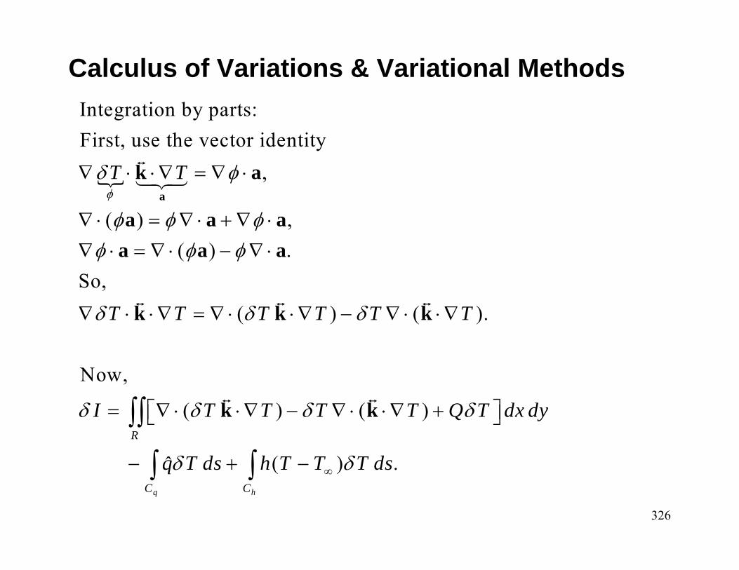
Calculus of Variations & Variational MethodsIntegration by parts:First, use the vector identity
,
( ) ,( ) .
So,( ) ( ).
Now,
( ) ( )
ˆR
T T
T T T T T T
I T T T T Q T dx dy
q T
φδ φ
φ φ φφ φ φ
δ δ δ
δ δ δ δ
δ
∇ ⋅ ⋅∇ = ∇ ⋅
∇ ⋅ = ∇ ⋅ + ∇ ⋅∇ ⋅ = ∇ ⋅ − ∇ ⋅
∇ ⋅ ⋅∇ = ∇ ⋅ ⋅∇ − ∇ ⋅ ⋅∇
= ∇ ⋅ ⋅∇ − ∇ ⋅ ⋅∇ +⎡ ⎤⎣ ⎦
−
∫∫
a
k a
a a aa a a
k k k
k k
( ) .q hC C
ds h T T T dsδ∞+ −∫ ∫
327
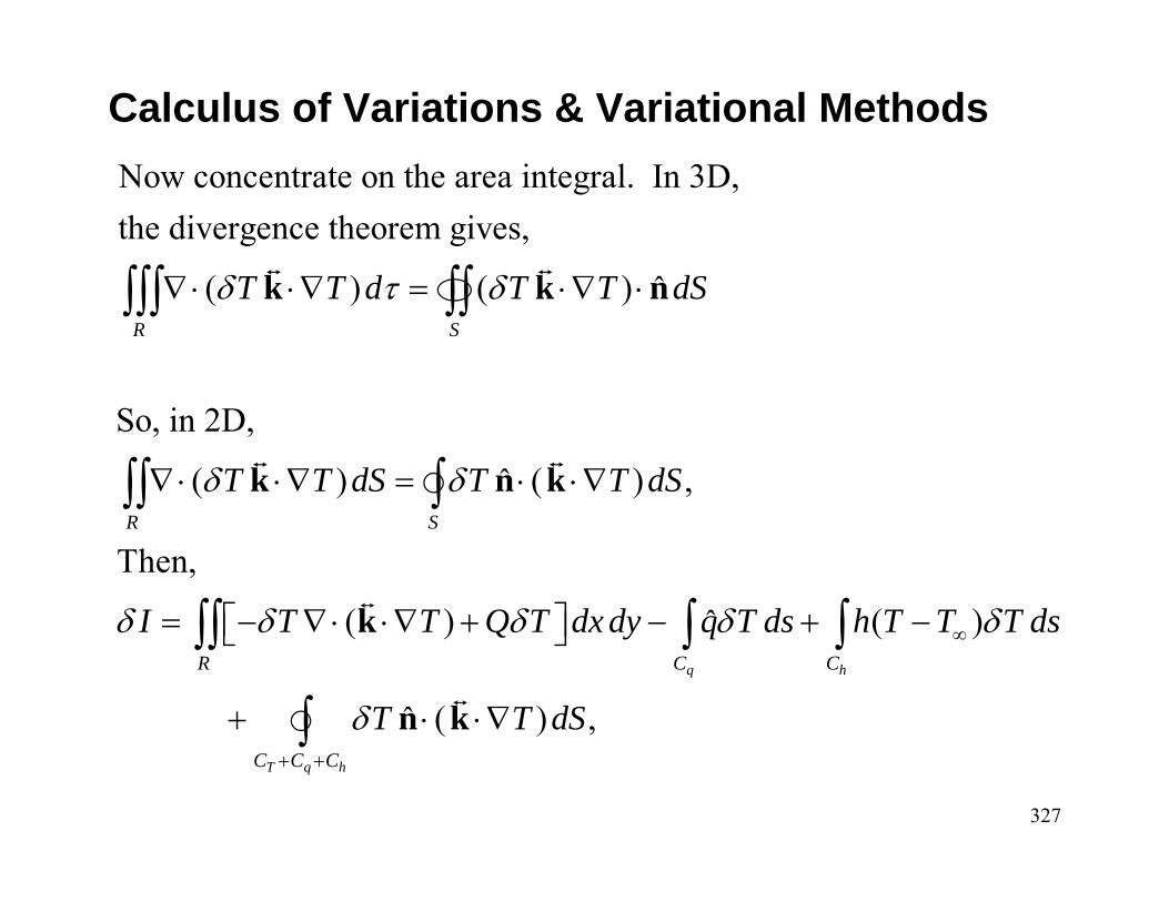
Calculus of Variations & Variational MethodsNow concentrate on the area integral. In 3D,the divergence theorem gives,
( ) ( ) ˆ
So, in 2D,
( ) ( ) ,ˆ
Then,
( ) ˆq
R S
R S
R C
T T d T T dS
T T dS T T dS
I T T Q T dx dy q T ds
δ τ δ
δ δ
δ δ δ δ
∇⋅ ⋅∇ = ⋅∇ ⋅
∇ ⋅ ⋅∇ = ⋅ ⋅∇
= − ∇⋅ ⋅∇ + −⎡ ⎤⎣ ⎦
∫∫∫ ∫∫
∫∫ ∫
∫∫ ∫
k k n
k n k
k ( )
( ) ,ˆh
T q h
C
C C C
h T T T ds
T T dS
δ
δ
∞
+ +
+ −
+ ⋅ ⋅∇
∫
∫ n k
328
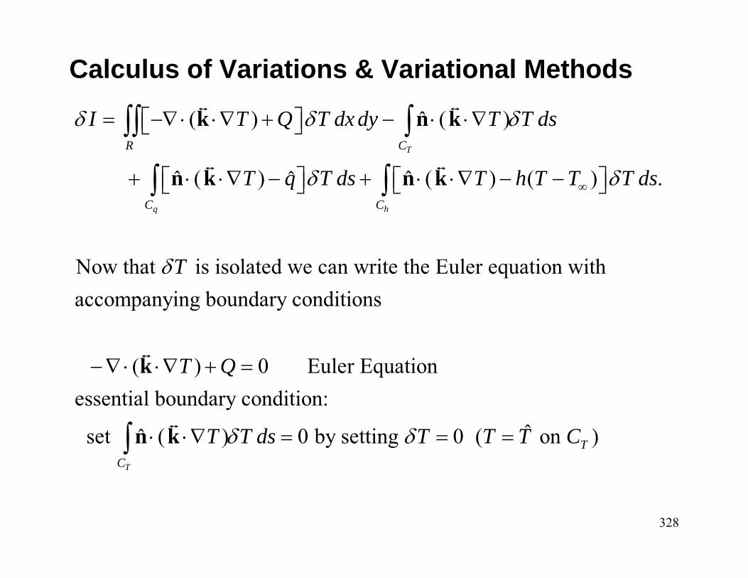
Calculus of Variations & Variational Methods
( ) ( )ˆ
( ) ( ) ( ) .ˆ ˆˆ
Now that is isolated we can write the Euler equation withaccompanying boundary conditi
T
q h
R C
C C
I T Q T dx dy T T ds
T q T ds T h T T T ds
T
δ δ δ
δ δ
δ
∞
= −∇⋅ ⋅∇ + − ⋅ ⋅∇⎡ ⎤⎣ ⎦
+ ⋅ ⋅∇ − + ⋅ ⋅∇ − −⎡ ⎤ ⎡ ⎤⎣ ⎦ ⎣ ⎦
∫∫ ∫
∫ ∫
k n k
n k n k
ons
( ) 0 Euler Equationessential boundary condition:
ˆ set ( ) 0 by setting 0 ( on )ˆT
TC
T Q
T T ds T T T Cδ δ
−∇⋅ ⋅∇ + =
⋅ ⋅∇ = = =∫
k
n k
329
Calculus of Variations & Variational Methods• Multiple Dependent Variables
So far we looked at the case where the functional is a function of one dependent variable, i.e., I(u). (Note, u is a dependent variable since it depends on x.) Now we look at the case I(u,v) where the functional is a function of two dependent variables.
The following development is for the 2D case, leaving the 3D case as an obvious extension. Begin with the functional to be minimized
( , ) ( , , , , , , , )x x y yR
I u v F x y u v u v u v dx dy= ∫∫
330
Calculus of Variations & Variational Methods
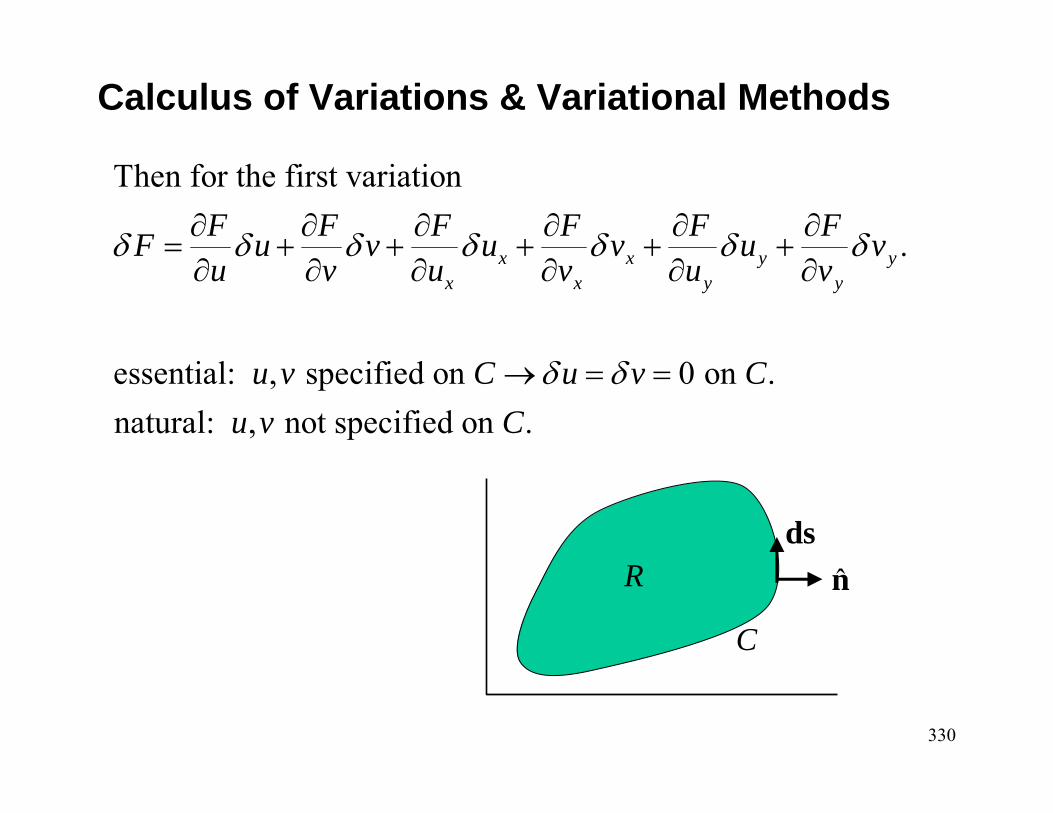
Then for the first variation
.
essential: , specified on 0 on .natural: , not specified on .
x x y yx x y y
F F F F F FF u v u v u vu v u v u v
u v C u v Cu v C
δ δ δ δ δ δ δ
δ δ
∂ ∂ ∂ ∂ ∂ ∂= + + + + +∂ ∂ ∂ ∂ ∂ ∂
→ = =
R
C
dsn̂
331
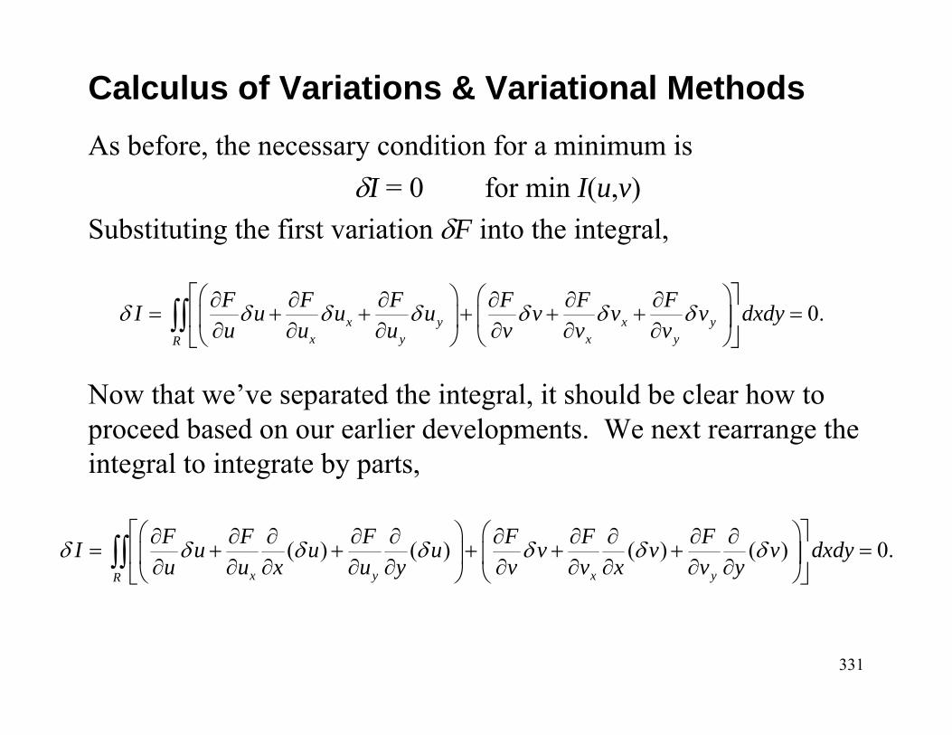
Calculus of Variations & Variational MethodsAs before, the necessary condition for a minimum is
δI = 0 for min I(u,v)Substituting the first variation δF into the integral,
Now that we’ve separated the integral, it should be clear how to proceed based on our earlier developments. We next rearrange the integral to integrate by parts,
0.x y x yx y x yR
F F F F F FI u u u v v v dxdyu u u v v v
δ δ δ δ δ δ δ⎡ ⎤⎛ ⎞ ⎛ ⎞∂ ∂ ∂ ∂ ∂ ∂= + + + + + =⎢ ⎥⎜ ⎟ ⎜ ⎟∂ ∂ ∂ ∂ ∂ ∂⎝ ⎠ ⎝ ⎠⎣ ⎦
∫∫
( ) ( ) ( ) ( ) 0.x y x yR
F F F F F FI u u u v v v dxdyu u x u y v v x v y
δ δ δ δ δ δ δ⎡ ⎤⎛ ⎞ ⎛ ⎞∂ ∂ ∂ ∂ ∂ ∂ ∂ ∂ ∂ ∂= + + + + + =⎢ ⎥⎜ ⎟ ⎜ ⎟∂ ∂ ∂ ∂ ∂ ∂ ∂ ∂ ∂ ∂⎝ ⎠ ⎝ ⎠⎣ ⎦
∫∫
332
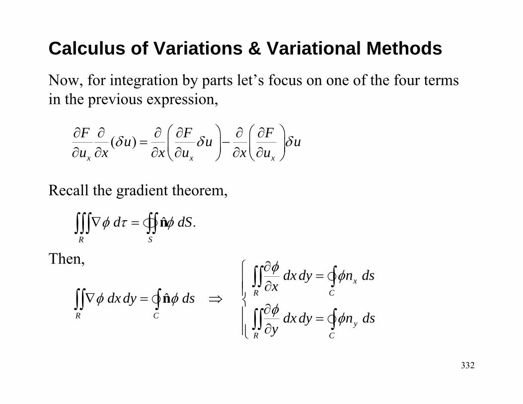
Calculus of Variations & Variational MethodsNow, for integration by parts let’s focus on one of the four terms in the previous expression,
Recall the gradient theorem,
Then,
( )x x x
F F Fu u uu x x u x u
δ δ δ⎛ ⎞ ⎛ ⎞∂ ∂ ∂ ∂ ∂ ∂= −⎜ ⎟ ⎜ ⎟∂ ∂ ∂ ∂ ∂ ∂⎝ ⎠ ⎝ ⎠
.ˆR S
d dSφ τ φ∇ =∫∫∫ ∫∫ n
ˆR C
dx dy dsφ φ∇ = ⇒∫∫ ∫ nx
R C
yR C
dx dy n dsx
dx dy n dsy
φ φ
φ φ
∂⎧ =⎪ ∂⎪⎨ ∂⎪ =
∂⎪⎩
∫∫ ∫
∫∫ ∫
333
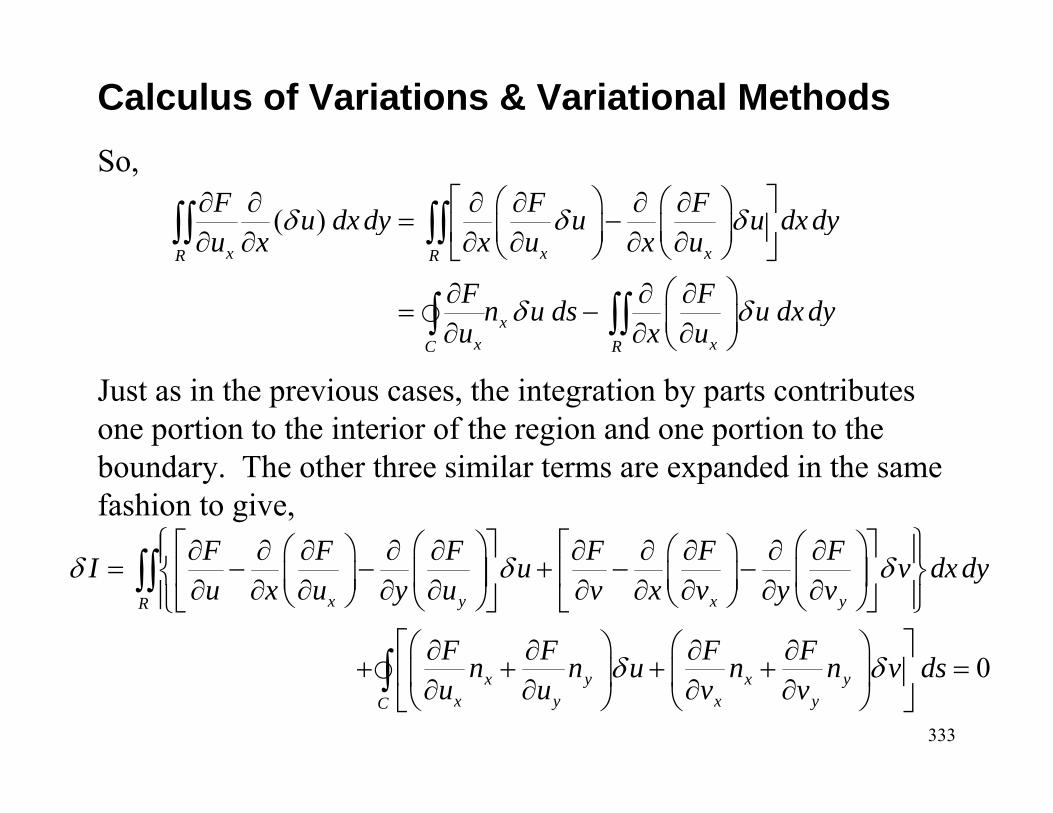
Calculus of Variations & Variational MethodsSo,
Just as in the previous cases, the integration by parts contributes one portion to the interior of the region and one portion to theboundary. The other three similar terms are expanded in the same fashion to give,
( )x x xR R
xx xC R
F F Fu dx dy u u dx dyu x x u x u
F Fn u ds u dx dyu x u
δ δ δ
δ δ
⎡ ⎤⎛ ⎞ ⎛ ⎞∂ ∂ ∂ ∂ ∂ ∂= −⎢ ⎥⎜ ⎟ ⎜ ⎟∂ ∂ ∂ ∂ ∂ ∂⎝ ⎠ ⎝ ⎠⎣ ⎦⎛ ⎞∂ ∂ ∂= − ⎜ ⎟∂ ∂ ∂⎝ ⎠
∫∫ ∫∫
∫ ∫∫
0
x y x yR
x y x yx y x yC
F F F F F FI u v dx dyu x u y u v x v y v
F F F Fn n u n n v dsu u v v
δ δ δ
δ δ
⎧ ⎫⎡ ⎤ ⎡ ⎤⎛ ⎞ ⎛ ⎞⎛ ⎞ ⎛ ⎞∂ ∂ ∂ ∂ ∂ ∂ ∂ ∂ ∂ ∂⎪ ⎪= − − + − −⎨ ⎬⎢ ⎥ ⎢ ⎥⎜ ⎟ ⎜ ⎟⎜ ⎟ ⎜ ⎟∂ ∂ ∂ ∂ ∂ ∂ ∂ ∂ ∂ ∂⎝ ⎠ ⎝ ⎠⎪ ⎪⎝ ⎠ ⎝ ⎠⎣ ⎦ ⎣ ⎦⎩ ⎭⎡ ⎤⎛ ⎞ ⎛ ⎞∂ ∂ ∂ ∂+ + + + =⎢ ⎥⎜ ⎟ ⎜ ⎟∂ ∂ ∂ ∂⎝ ⎠ ⎝ ⎠⎣ ⎦
∫∫
∫
334
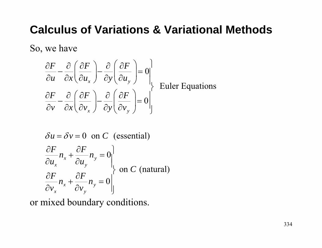
Calculus of Variations & Variational MethodsSo, we have
or mixed boundary conditions.
0
Euler Equations
0
0 on (essential)
0 on (natural)
0
x y
x y
x yx y
x yx y
F F Fu x u y u
F F Fv x v y v
u v CF Fn nu u
CF Fn nv v
δ δ
⎫⎛ ⎞⎛ ⎞∂ ∂ ∂ ∂ ∂− − = ⎪⎜ ⎟⎜ ⎟∂ ∂ ∂ ∂ ∂⎝ ⎠ ⎝ ⎠ ⎪⎬
⎛ ⎞⎛ ⎞∂ ∂ ∂ ∂ ∂ ⎪− − =⎜ ⎟⎜ ⎟ ⎪∂ ∂ ∂ ∂ ∂⎝ ⎠ ⎝ ⎠ ⎭
= =
∂ ∂ ⎫+ = ⎪∂ ∂ ⎪⎬∂ ∂ ⎪+ =
∂ ∂ ⎪⎭