Calculus and heat flow in metric measure spaces and spaces ... Ambrosio.pdf · Calculus and heat...

Calculus and heat flow in metric measure spacesand spaces with Riemannian curvature

bounds from below

L. Ambrosio

Scuola Normale Superiore, Pisahttp://cvgmt.sns.it

Luigi Ambrosio (SNS) Oxford, September 2012 1 / 31

A.-Gigli-Savaré: Calculus and heat flow in metric measure spaces(X ,d ,m) and applications to spaces with Ricci bounds from below.Goal. To develop a “calculus” in metric measure spaces, use it toidentify different notions of heat flow, and apply these results to theLott-Sturm-Villani metric measure spaces with Ricci curvature boundedfrom below.

A.-Gigli-Savaré: Metric measure spaces with Riemannian Riccicurvature bounded from below.Goal. Introduce a more restrictive and “Riemannian” notion of Riccibound from below for metric measure spaces, still consistent andstable under measured Gromov-Hausdorff limits, which rules outFinsler spaces.

(both available on http://cvgmt.sns.it, or ArXiv)

A.-Gigli-Savaré: Bakry-Emery condition and Riemannian Riccicurvature bounds (to appear).


MotivationsCheeger-Colding studied in detail limits, in the Gromov-Hausdorffsense, of sequences of Riemannian manifolds with given dimensionN and uniform lower bound K on Ricci tensor (with more recentcontributions by Colding-Naber, Honda). Even though many results(rectifiability, tangent spaces, etc.) are available, these limits aredescribed only in metric terms. Question: is there an intrinsic/richerdescription of these spaces? Can we develop intrinsic calculus tools(gradient, differential, heat flow,..)?

Can we relate the “Lagrangian" CD(K ,N) theory, developed byLott-Sturm-Villani, to the “Eulerian" cd(ρ,n) theory of Bakry-Emery?

One of the great merits of the first theory, based on optimaltransportation, is stability under GH limits, while the second one, basedon the theory of Markov semigroups and the so-called Γ-calculus, ismaybe more powerful in the derivation in sharp form of analytic andgeometric inequalities (Poincaré, logarithmic Sobolev, isoperimetric..).


Outline

1 Some by now “classical” results

2 Identification of weak gradients

3 Identification of gradient flows

4 Riemannian Ricci lower bounds


Some by now “classical” results

Let us consider in Rn the heat equation (ut (x) = u(t , x))

ddt

ut = ∆ut .

Classically, it can be viewed as the gradient flow of the energy

Dir(u) :=12

∫Rn|∇u|2 dx (+∞ if u /∈ H1(Rn))

in the Hilbert space H = L2(Rn).

Formally, t 7→ ut solves the ODE u′ = −∇Dir(u) in H because

Dir “differentiable” at u ⇐⇒ −∆u ∈ L2, ∇Dir(u) = −∆u.


In 1998, Jordan-Kinderlehrer-Otto proved that the same equationarises as gradient flow of the entropy functional

Ent(ρL n) :=

∫Rnρ log ρdx (+∞ if µ is not a.c. w.r.t. L n)

in the space P2(Rn) of probability measures with finite quadraticmoments, with respect to Wasserstein distance W2.

W 22 (µ, ν) := min

{∫Rn×Rn

|x − y |2 dγ(x , y) : (π1)]γ = µ, (π2)]γ = ν

}.

Push forward notation. f : X → Y Borel induces a mapf] : P(X )→P(Y ):

f]µ(B) := µ(f−1(B)

)∀B ∈ B(Y ).


The reason underlying the JKO result is that we may view P2(Rn) asan infinite-dimensional differentiable manifold, considering the tangentvector field vt to a curve (µt ) in P2(Rn) as the “velocity” occurring inthe continuity equation

ddtµt +∇ · (vtµt ) = 0, vt = ∇φt .

Then, defining the metric at µ ∈P2(Rn) as

〈v ,w〉µ :=

∫v(x) · w(x) dµ(x) v , w ∈ {∇φ : φ ∈ C∞c (Rn)}L

2(µ)

we turn P2(Rn) into a Riemannian manifold and it can be proved (Otto,Benamou-Brenier) that the induced distance is precisely W2.This discovery originated a huge literature, where many other diffusion(even of fourth order) and transport equations are viewed that way,with new existence and uniqueness results, rates of convergence toequilibrium, etc. In our papers we explore the potential of these ideasin a nonsmooth setting.


Proofs of this equivalence1. By the so-called Otto calculus, i.e. formally viewing P(Rn) asan infinite dimensional Riemannian manifold. Computing with thisstructure the gradient flow of Ent for µt = ρtL

n gives vt = ∇ log ρt .

2. Prove that the implicit time discretization scheme (Euler scheme),traditionally used for the time discrete approximation of gradient flows,when done with energy Ent and distance W2, does converge to theheat equation.

3. Give a meaning to what “gradient flow of Ent in P(Rn) w.r.t. W2means”, and check that solutions of this gradient flow are solutions tothe heat equation. Then, apply uniqueness for d

dt ut = ∆ut .

The last strategy is more abstract, but still uses the differentiablestructure of Rn. The question is to understand deeper reasons for thisequivalence, in particular on which structural properties of the spaceit depends (Riemannian manifolds, Finsler spaces, Wiener spaces,sub-Riemannian spaces, Alexandrov spaces, etc.)


Metric measure spacesLet us consider a metric measure space (X ,d ,m), with m ∈P(X ).In this framework it is still possible to define a “Dirichlet energy”, thatwe call Cheeger functional:

Ch(f ) :=12

inf{

lim infn→∞

∫X|∇fn|2 dm : fn ∈ Lip(X ),

∫X|fn − f |2 dm→ 0

},

where|∇g|(x) := lim sup

y→x

|g(y)− g(x)|d(y , x)

is the slope (also called local Lipschitz constant).Also, one can consider Shannon’s relative entropy functionalEntm : P(X )→ [0,+∞]

Entm(ρm) :=

∫Xρ log ρdm (+∞ if µ is not a.c. w.r.t. m).


The basic result is that the equivalence between L2-gradient flow ofCh and W2-gradient flow of Entm always holds, if the latter is properlyunderstood. But, without additional assumptions on the space, bothobjects can be trivial.Example. Let X = [0,1], d the Euclidean distance, m =

∑n≥1 2−nδqn ,

where {qn}n≥1 is an enumeration of [0,1]∩Q. Let An ⊃ Q∩X be opensets with L 1(An)→ 0 and

χn(t) :=

∫ t

0

(1− χAn (s)

)ds t ∈ [0,1].

Then f ◦ χn → f in L2(X ,m) for all f ∈ Lip(X ) and f ◦ χn is locallyconstant in Q ∩ X hence

Ch(f ) = 0 ∀f ∈ Lip(X ).

It follows that Ch ≡ 0 in L2(X ,m).


Identification of weak gradientsA closely related question, relevant in particular for the second paper,is the identification of weak gradients. The first one, that we call relaxedgradient |∇f |∗, is the object that provides integral representation to Ch:

Ch(f ) =12

∫X|∇f |2∗ dm ∀f ∈ D(Ch).

It has all the natural properties a weak gradient should have, forinstance locality

f = g on B =⇒ |∇f |∗ = |∇g|∗ m-a.e. in B

and chain rule

|∇(φ ◦ f )|∗ = |φ′(f )||∇f |∗ m-a.e. in X .

This gradient is useful when doing “vertical” variations ε 7→ f + εg(i.e. in the dependent variable).


Identification of weak gradients

But, when computing variations of the entropy, the “horizontal”variations ε → f (γε) (i.e. in the independent variable) are necessary.These are related to another weak gradient |∇f |w , defined as follows.Let us recall, first, the notion of upper gradient (Heinonen-Koskela): itis a function G satisfying

(∗) |f (γ1)− f (γ0)| ≤∫γ

G

on all absolutely continuous curves γ. Obviously G ≥ |∇f | in a“smooth” setting and the smallest upper gradient is precisely |∇f |.We consider the so-called weak upper gradient property by requiring (*)along “almost all” curves γ in AC2([0,1]; X ). Then, we define |∇f |w asthe weak upper gradient G with smallest L2(X ,m) norm. This is relatedto a notion introduced by Koskela-MacManus, Shanmugalingham, butwith a different notion of null set of curves.


Null sets of curvesWe say that a (Borel) set Γ of absolutely continuous curvesγ : [0,1]→ X is null if

π(Γ) = 0 for any test plan π.

Here, the class of test plans is simply the collection of allπ ∈P(AC2([0,1]; X )) satisfying

(et )]π ≤ Cm ∀t ∈ [0,1] for some C = C(π) ≥ 0.

Theorem. In any complete and separable metric measure space(X ,d ,m) with m finite on bounded sets the relaxed gradient |∇f |∗ andthe minimal weak upper gradient |∇f |w coincide m-a.e. in X.Of course, maybe they are both trivial without extra assumptions.The proof of this identification uses ideas from optimal transportation,as lifting of solutions to the heat flow to probability measures inAC2([0,1]; X

)and the energy dissipation rate of Entm.


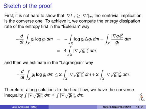
Sketch of the proof

First, it is not hard to show that |∇f |∗ ≥ |∇f |w , the nontrivial implicationis the converse one. To achieve it, we compute the energy dissipationrate of the entropy first in the “Eulerian" way

− ddt

∫X

gt log gt dm = −∫

Xlog gt ∆gt dm =

∫X

|∇gt |2∗gt

dm

= 4∫

X|∇√

gt |2∗ dm.

and then we estimate in the “Lagrangian" way

− ddt

∫X

gt log gt dm ≤ 2∫

X|∇√

gt |2∗ dm + 2∫

X|∇√

gt |2w dm.

Therefore, along solutions to the heat flow, we have the converseinequality

∫|∇√gt |2∗ dm ≤

∫|∇√gt |2w dm.


Equivalence of gradient flowsWe assume in this section that the metric measure space (X ,d ,m)satisfies ∫

Xe−V 2(x) dm(x) <∞

for some Lipschitz weight function V : X → R. It surely holds withV (x) = d(x , x0) if m(B(x0, r)) ≤ Cec r2

. We also define the descendingslope of the entropy

|∇−Entm|(µ) := lim supν→µ

[Entm(µ)− Entm(ν)]+

W2(ν, µ)

and we assume that the conditions

supn

Entm(ρnm) <∞, ρnm ⇀ ρm, limn→∞

∫X

V 2ρn dm =

∫X

V 2ρdm,

implylim infn→∞

|∇−Entm|(ρnm) ≥ |∇−Entm|(ρm)

and that |∇−Entm| is an upper gradient of Entm. These properties ofthe slope are fulfilled in all CD(K ,∞) spaces.


Lott-Sturm-Villani CD(K ,∞) spacesIn these spaces (I consider only the case N = ∞) one requires K -convexity along Wasserstein geodesics, namely for all µ0, µ1 ∈ D(Entm)there exists a constant speed geodesic µt satisfying

Entm(µt ) ≤ (1− t)Entm(µ0) + tEntm(µ1)− K2

t(1− t)W 22 (µ0, µ1).

When (X ,d) is a Riemannian manifold, CD(K ,∞) holds iff RicX ≥ KI(Cordero-McCann-Schmuckenschläger, Sturm-Von Renesse).Consequences of convexity:• Duality formula for the slope (here stated for K = 0):

|∇−Entm|(µ) = supν 6=µ

[Entm(µ)− Entm(ν)]+

W2(µ, ν).

It implies, among other things, that µ 7→ |∇−Entm|(µ) is l.s.c.• Upper gradient property. The previous formula for the slope implies aone-sided and local Lipschitz estimate

Entm(µt )− Entm(µs) ≤ |∇−Ent|(µt )W2(µt , µs).


Equivalence of gradient flows

Theorem. Let ρ0 ∈ L2(X ,m) be a probability density and let ρt be theL2-gradient flow of Ch starting from ρ0. Then ρt is a probability densityfor all t ≥ 0 and ρtm is the W2-gradient flow of Entm starting from f0m.Conversely, if µ0 = ρ0m with ρ0 ∈ L2(X ,m) and µt is the W2-gradientflow of Entm starting from µ0, then µt = ρtm for all t ≥ 0.Finally, the energy dissipation rates coincide:

4∫

X|∇√ρt |2∗ dm = |∇−Entm|2(ρtm) for a.e. t > 0.

Corollary. (Fisher information functional and slope of Entm coincide)

4∫

X|∇√ρ|2∗ dm = |∇−Entm|2(ρm).


Equivalence of gradient flows

The proof of the theorem consists of the following two steps:(1) inclusion of L2-gradient flows into W2-gradient flows;(2) uniqueness of W2-gradient flows.This strategy, borrowed from Gigli-Kuwada-Ohta, reverses the usualone adopted in Rn, Riemannian manifolds and other “smooth” spaces.Part (2), a key point in the new strategy, is due to Gigli. Notice howeverthat contractivity of W2 may fail (Ohta-Sturm) (an open problem is tofind whether contractivity holds for other better adapted distances).I will now focus on the meaning of L2- and W2- gradient flows andexplain briefly (1).


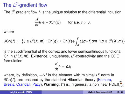
The L2-gradient flowThe L2 gradient flow ft is the unique solution to the differential inclusion

ddt

ft ∈ −∂Ch(ft ) for a.e. t > 0,

where

∂Ch(f ) :={ξ ∈ L2(X ,m) : Ch(g) ≥ Ch(f )+

∫Xξ(g−f )dm ∀g ∈ L2(X ,m)

}is the subdifferential of the convex and lower semicontinuous functionalCh in L2(X ,m). Existence, uniqueness, L2-contractivity and the ODEformulation

ddt

ft = ∆ft

where, by definition, −∆f is the element with minimal L2 norm in∂Ch(f ), are ensured by the standard Hilbertian theory (Komura,Brezis, Crandall, Pazy). Warning: (*) is, in general, a nonlinear PDE!!


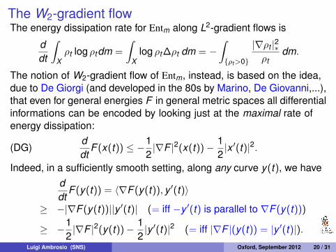
The W2-gradient flowThe energy dissipation rate for Entm along L2-gradient flows is

ddt

∫Xρt log ρtdm =

∫X

log ρt ∆ρt dm = −∫{ρt>0}

|∇ρt |2∗ρt

dm.

The notion of W2-gradient flow of Entm, instead, is based on the idea,due to De Giorgi (and developed in the 80s by Marino, De Giovanni,...),that even for general energies F in general metric spaces all differentialinformations can be encoded by looking just at the maximal rate ofenergy dissipation:

(DG)ddt

F (x(t)) ≤ −12|∇F |2(x(t))− 1

2|x ′(t)|2.

Indeed, in a sufficiently smooth setting, along any curve y(t), we haveddt

F (y(t)) = 〈∇F (y(t)), y ′(t)〉

≥ −|∇F (y(t))||y ′(t)| (= iff −y ′(t) is parallel to ∇F (y(t)))

≥ −12|∇F |2(y(t))− 1

2|y ′(t)|2 (= iff |∇F |(y(t)) = |y ′(t)|).


The W2-gradient flow

(DG)ddt

F (x(t)) ≤ −12|∇F |2(x(t))− 1

2|x ′(t)|2.

All terms in (DG) make sense in a metric space (Y ,dY ): |x ′| can bereplaced by the metric derivative

|x ′|(t) := lims→t

dY (x(s), x(t))

|s − t |

and |∇F | by the descending slope |∇−F |, so that the speed is 0 atminimum points.Coming back to the case (Y ,dY ) = (P2(X ),W2), F = Entm, to convertL2-heat flows to W2-gradient flows we need to bound both the metricderivative of t 7→ ρtm and the descending slope of Entm(ρt ) with theL2-energy dissipation rate.


Kuwada’s lemma (from Gigli-Kuwada-Ohta ’10)

Lemma. Let ρ0 ∈ L2(X ,m) a probability density, ρt the L2-gradient flowstarting from ρ0. Then the curve µt := ρtm is absolutely continuous inP2(X ) and

|µ̇t |2 ≤∫{ρt>0}

|∇ρt |2∗ρt

dm for a.e. t > 0.

The proof of the Lemma, that we extended to all metric measurespaces, requires a fine analysis of the differentiability properties ofsolutions Qt f of the Hopf-Lax semigroup

Qt f (x) := infy∈X

f (y) +12t

d2(x , y),ddt

Qt f (x) +12|∇Qt f |2(x) ≤ 0.

These solutions describe (Bernard-Buffoni, Lott-Villani) the evolution intime of Kantorovich potentials.


Riemannian Ricci lower boundsAs shown by Cordero Erausquin-Sturm-Villani, all Minkowski spaces(Rn endowed with the Lebesgue measure and any norm ‖ · ‖) satisfythe CD(0,n) (and therefore the CD(0,∞)) condition. On the otherhand, Cheeger-Colding ruled out the possibility to obtain these spacesas limits of Riemannian manifolds.Question. Is there a more restrictive notion, still stable and (strongly)consistent with the Riemannian case, that rules out Minkowski (andthen Finsler) spaces?Definition. We say that (X ,d ,m), with m(X ) < ∞, has RiemannianRicci curvature bounded from below by K ∈ R, and write RCD(K ,∞),if one of the following equivalent conditions hold:

(i) (X ,d ,m) is a CD(K ,∞) space and the L2 heat flow ht is linear;(ii) (X ,d ,m) is a CD(K ,∞) space and the W2 heat flow Ht is additive

(i.e. convex and concave) on P2(X );(iii) for all µ ∈P2(X ) with suppµ ⊂ supp m, Htµ is a gradient flow in

the EVIK sense.


Properties of RCD(K ,∞) spaces

• Stability under measured Gromov-Hausdorff limits. Here we can workwith the same notions of isomorphim between metric measure spacesand distance between isomorphism classes introduced by Sturm. Inthe proof of this result it is the EVIK formulation that plays a decisiverole.• Tensorization. If (X ,dX ,mX ) and (Y ,dY ,mY ) are RCD(K ,∞), so is

(X × Y ,√

d2X + d2

Y ,mX ×mY ). Here we can remove the non branchingassumption of the CD(K ,N) theory.• Fine properties of the heat flow. The identification between the L2

heat flow ht and the W2 heat flow Ht allows to pick the best propertiesfrom each of them: for instance, the symmetry of the transitionprobabilities θt : X × X → [0,∞), defined by Htδx := θt (x , ·)m, comesfrom the fact that ht is L2-selfadjoint, while the contractivity propertiesof ht in spaces different from Lp(X ,m) follow from those of Ht .


More properties of the heat flow

(1) The pointwise formula h̃t f (x) :=∫

f dHtδx provides a version ofht f and an extension of ht to a contraction semigroup in all Lp(X ,m)spaces.(2) h̃t leaves Lip(supp m) invariant and Lip(h̃t f ) ≤ e−KtLip(f ) (itfollows by the contractivity estimate W2(Htδx ,Htδy ) ≤ e−Ktd(x , y)).Furthermore, h̃t maps L∞(X ,m) in Cb(supp m).(3) The Bakry-Emery estimate holds:

(BEK ,∞) |∇(ht f )|2∗ ≤ e−2Ktht |∇f |2∗ m-a.e. in X .


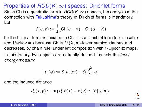
Properties of RCD(K ,∞) spaces: Dirichlet formsSince Ch is a quadratic form in RCD(K ,∞) spaces, the analysis of theconnection with Fukushima’s theory of Dirichlet forms is mandatory.Let

E(u, v) :=14(Ch(u + v)− Ch(u − v)

)be the bilinear form associated to Ch. It is a Dirichlet form (i.e. closableand Markovian) because Ch is L2(X ,m)-lower semicontinuous anddecreases, by chain rule, under left composition with 1-Lipschitz maps.In this theory, two objects are naturally defined, namely the localenergy measure

[u](ϕ) := E(u,uϕ)− E(u2

2, ϕ)

and the induced distance

dE(x , y) := sup {|ψ(x)− ψ(y)| : [ψ] ≤ m} .


Properties of RCD(K ,∞) spaces: Dirichlet formsTheorem. In a RCD(K ,∞) space (X ,d ,m) the local energy measure[u] coincides with |∇u|2∗m and the induced distance dE coincides withd.The proof involves the construction of a symmetric bilinear form

(u, v) ∈[D(Ch)

]2 7→ ∇u · ∇v ∈ L1(X ,m)

satisfying the Leibnitz rule and providing integral representation to E ,namely E(u, v) =

∫∇u · ∇v dm.

In addition, since E is also strongly local, the theory of Dirichlet forms(Fukushima, Ma-Röckner) can be applied to obtain a unique (in law)Brownian motion in (supp m,d ,m), i.e. a Markov process X t withcontinuous sample paths satisfying

P(X t |X 0 = x) = Htδx ∀x ∈ supp m, t ≥ 0.


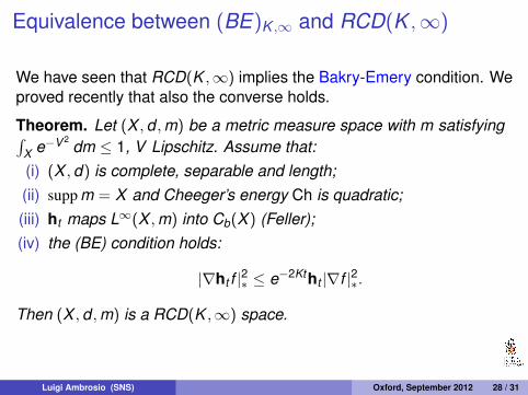
Equivalence between (BE)K ,∞ and RCD(K ,∞)

We have seen that RCD(K ,∞) implies the Bakry-Emery condition. Weproved recently that also the converse holds.

Theorem. Let (X ,d ,m) be a metric measure space with m satisfying∫X e−V 2

dm ≤ 1, V Lipschitz. Assume that:(i) (X ,d) is complete, separable and length;(ii) supp m = X and Cheeger’s energy Ch is quadratic;(iii) ht maps L∞(X ,m) into Cb(X ) (Feller);(iv) the (BE) condition holds:

|∇ht f |2∗ ≤ e−2Ktht |∇f |2∗.

Then (X ,d ,m) is a RCD(K ,∞) space.


The EVI formulation of gradient flowsIf H is Hilbert and F : X → R ∪ {+∞} is K -convex and l.s.c., wecan write the differential inclusion −x ′(t) ∈ ∂F (x(t)) for a.e. t > 0 asfollows:

∀y , 〈−x ′(t), y − x(t)〉+K2|(x(t)− y |2 + F (x(t)) ≤ F (y) for a.e. t > 0.

Equivalently

∀y , ddt

12|x(t)− y |2 +

K2|(x(t)− y |2 + F (x(t)) ≤ F (y) for a.e. t > 0.

Definition. In a metric space (E ,d), a locally absolutely continuouscurve u : (0,∞) → E is an EVIK solution to the gradient flow ofF : X → R ∪ {+∞} if for all v ∈ D(F ) it holds

ddt

12

d2(u(t), v) +K2|(u(t)− v |2F (u(t)) ≤ F (v) for a.e. t > 0.

This formulation of gradient flows is equivalent in Hilbert spaces, but ingeneral stronger than the one based on energy dissipation (Savaré).


Open problems and perspectives(1) For the dimensional theory, i.e. N < ∞, we expect similarconnections in the case K = 0 between convexity of the Renyi entropy

EN(ρ) := −∫

Xρ1−1/N dm µ = ρm + µs, µs ⊥ m

the N-dimensional Bakry-Emery condition

(BE0,N) |∇(ht f )|2∗ +t2

N(∆ht f )2 ≤ ht |∇f |2∗ m-a.e. in X .

and Bochner’s inequality

∆|∇f |2∗

2≥ 〈∇∆f ,∇f 〉+

(∆f )2

N.

But, the case CD(K ,N) with N < ∞ and K 6= 0 seems to be muchmore problematic.(2) What about nonlocal diffusions? Recent work in Rn by Erbar showsthat the Otto equivalence persists, properly understood. In this caseW2 has to be replaced by the distance arising by the minimization of asuitable action functional, in the spirit of Benamou-Brenier.


Open problems and perspectives

(3) In presence of doubling & Poincaré, Cheeger’s theory applies andprovides, in a suitable and very weak sense, local coordinates and atangent bundle. The relations with the calculus described in this lectureare still not completely understood.(4) What about the behaviour on small scales of RCD(K ,∞) spaces?The question makes sense, if one adds a doubling condition on themeasure m. The natural conjecture is that tangent metric spaces, inthe measured GH sense, are Euclidean. This has been proved byCheeger-Colding, but for limits of Riemannian manifolds, there is workin progress by Gigli in the RCD(K ,∞) framework.

Thank you for the attention!


Calculus and heat flow in metric measure spaces and spaces ... Ambrosio.pdf · Calculus and heat...

Documents

Transcript of Calculus and heat flow in metric measure spaces and spaces ... Ambrosio.pdf · Calculus and heat...