Calculus
222
Calculus: Early Transcendental Functions Lecture Notes for Calculus 101 Feras Awad Mahmoud Last Updated: January 22, 2012 1
-
Upload
jefferson-dias -
Category
Documents
-
view
243 -
download
14
Transcript of Calculus
Calculus: Early Transcendental FunctionsLecture Notes for Calculus 101
Feras Awad Mahmoud
Last Updated: January 22, 2012
1

2
Feras Awad MahmoudDepartment of Basic SciencesPhiladelphia UniversityJORDAN 19392
Textbook:This book is strongly recommended for Calculus 101 as well asa reference text for Calculus 102. The pdf soft−copy of the fivechapters remain available for free download.
Typesetting:The entire document was written in LaTeX, implemented forWindows using the MiKTeX 2.9 distribution. As for the texteditor of my choice, I fancy WinEdt 6.0.
Moral Support:My wife has had a very instrumental role in providing moralsupport. Thank God for her patience, understanding, encour-agement, and prayers throughout the long process of writingand editing.
c©2012 Feras Awad Mahmoud. All Rights Reserved.www.philadelphia.edu.jo/academics/fawad

Contents
Contents 3
1 Functions 51.1 Introduction . . . . . . . . . . . . . . . . . . . . . . . . . . . 51.2 Essential Functions . . . . . . . . . . . . . . . . . . . . . . . 91.3 Combinations of Functions . . . . . . . . . . . . . . . . . . . 261.4 Inverse Functions . . . . . . . . . . . . . . . . . . . . . . . . 301.5 Hyperbolic Functions . . . . . . . . . . . . . . . . . . . . . . 53
2 Limits and Continuity 572.1 An Introduction to Limits . . . . . . . . . . . . . . . . . . . 572.2 Calculating Limits using the Limit Laws . . . . . . . . . . . 642.3 Limits at Infinity and Infinite Limits . . . . . . . . . . . . . 732.4 Limits Involving (sin θ) /θ . . . . . . . . . . . . . . . . . . . 862.5 Continuous Functions . . . . . . . . . . . . . . . . . . . . . . 89
3 The Derivative 973.1 The Derivative as a Function . . . . . . . . . . . . . . . . . . 973.2 Differentiation Rules and Higher Derivatives . . . . . . . . . 1033.3 The Chain Rule . . . . . . . . . . . . . . . . . . . . . . . . . 1133.4 Implicit Differentiation . . . . . . . . . . . . . . . . . . . . . 1193.5 Tangent Line . . . . . . . . . . . . . . . . . . . . . . . . . . 122
4 Applications of Differentiation 127
3
4 CONTENTS
4.1 Indeterminate Forms and L’Hospital’s Rule . . . . . . . . . . 1274.2 The Mean Value Theorem . . . . . . . . . . . . . . . . . . . 1344.3 Extreme Values of Functions . . . . . . . . . . . . . . . . . . 1394.4 Monotonic Functions . . . . . . . . . . . . . . . . . . . . . . 1464.5 Concavity and Curve Sketching . . . . . . . . . . . . . . . . 151
5 Integration 1595.1 Antiderivatives . . . . . . . . . . . . . . . . . . . . . . . . . 1595.2 Indefinite Integrals . . . . . . . . . . . . . . . . . . . . . . . 1605.3 Integration by Substitution . . . . . . . . . . . . . . . . . . . 1705.4 The Definite Integral . . . . . . . . . . . . . . . . . . . . . . 1755.5 The Fundamental Theorem of Calculus . . . . . . . . . . . . 1815.6 Area Between Two Curves . . . . . . . . . . . . . . . . . . . 188
A Solving Equations and Inequalities 195
B Absolute Value 207
C Equation of Line 211
D Final Answers of Exercises 217
Chapter 1
Functions
1.1 Introduction
Functions arise whenever one quantity depends on another.
Definition 1.1.1. A function f is a rule that assigns to each element xin a set D exactly one element called f(x) in a set E.
• We usually consider functions for which the sets D and E are sets ofreal numbers.
• The set D is called the domain of the function.
• The number f(x) is the value of f at x and is read f of x.
• The range of f is the set of all possible values of f(x) as x variesthroughout the domain
• A symbol that represents an arbitrary number in the domain of afunction f is called an independent variable.
• A symbol that represents a number in the range of f is called a de-pendent variable.
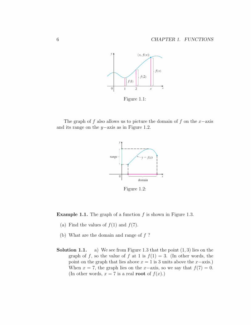
Since the y−coordinate of any point (x, y) on the graph is y = f(x), wecan read the value of f(x) from the graph as being the height of the graphabove the point x (see Figure 1.1).
5
6 CHAPTER 1. FUNCTIONS
Figure 1.1:
The graph of f also allows us to picture the domain of f on the x−axisand its range on the y−axis as in Figure 1.2.
Figure 1.2:
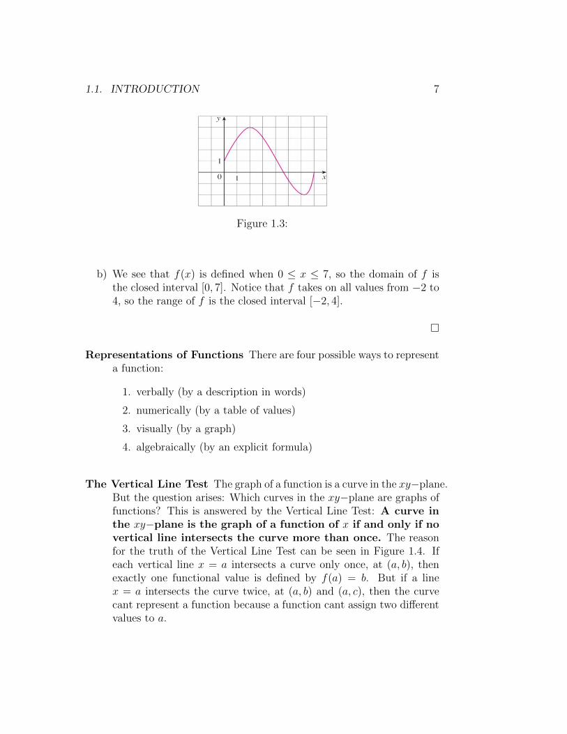
Example 1.1. The graph of a function f is shown in Figure 1.3.
(a) Find the values of f(1) and f(7).
(b) What are the domain and range of f ?
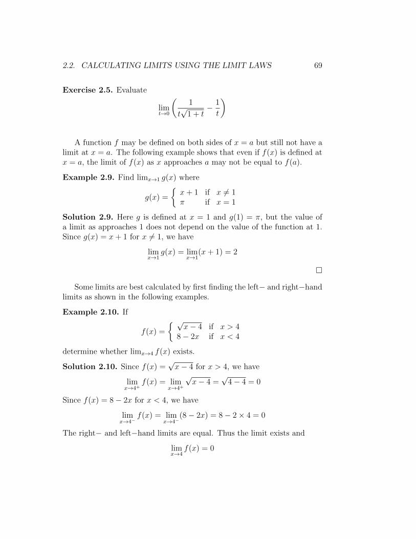
Solution 1.1. a) We see from Figure 1.3 that the point (1, 3) lies on thegraph of f , so the value of f at 1 is f(1) = 3. (In other words, thepoint on the graph that lies above x = 1 is 3 units above the x−axis.)When x = 7, the graph lies on the x−axis, so we say that f(7) = 0.(In other words, x = 7 is a real root of f(x).)
1.1. INTRODUCTION 7
Figure 1.3:
b) We see that f(x) is defined when 0 ≤ x ≤ 7, so the domain of f isthe closed interval [0, 7]. Notice that f takes on all values from −2 to4, so the range of f is the closed interval [−2, 4].
�
Representations of Functions There are four possible ways to representa function:
1. verbally (by a description in words)
2. numerically (by a table of values)
3. visually (by a graph)
4. algebraically (by an explicit formula)
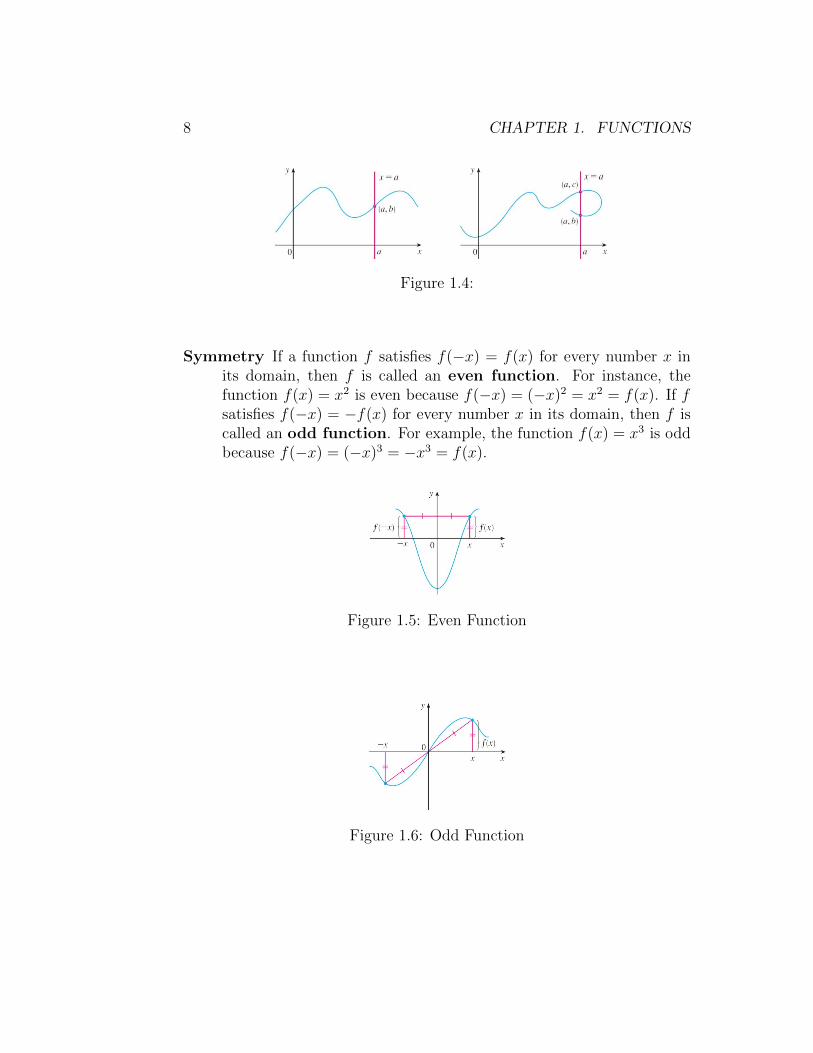
The Vertical Line Test The graph of a function is a curve in the xy−plane.But the question arises: Which curves in the xy−plane are graphs offunctions? This is answered by the Vertical Line Test: A curve inthe xy−plane is the graph of a function of x if and only if novertical line intersects the curve more than once. The reasonfor the truth of the Vertical Line Test can be seen in Figure 1.4. Ifeach vertical line x = a intersects a curve only once, at (a, b), thenexactly one functional value is defined by f(a) = b. But if a linex = a intersects the curve twice, at (a, b) and (a, c), then the curvecant represent a function because a function cant assign two differentvalues to a.
8 CHAPTER 1. FUNCTIONS
Figure 1.4:
Symmetry If a function f satisfies f(−x) = f(x) for every number x inits domain, then f is called an even function. For instance, thefunction f(x) = x2 is even because f(−x) = (−x)2 = x2 = f(x). If fsatisfies f(−x) = −f(x) for every number x in its domain, then f iscalled an odd function. For example, the function f(x) = x3 is oddbecause f(−x) = (−x)3 = −x3 = f(x).
Figure 1.5: Even Function
Figure 1.6: Odd Function

1.2. ESSENTIAL FUNCTIONS 9
The geometric significance of an even function is that its graph is symmetricwith respect to the y−axis as in Figure 1.5, while the graph of an oddfunction is symmetric about the origin, see Figure 1.6.
Example 1.2. Determine whether each of the following functions is even,odd, or neither even nor odd.
(a) f(x) = x5 + x.
(b) g(x) = 1− x4.
(c) h(x) = 2x− x2.
Solution 1.2. (a) f(−x) = (−x)5+(−x) = (−1)5x5+(−x) = −x5−x =−(x5 + x) = −f(x). Therefore f is an odd function.
(b) g(−x) = 1− (−x)4 = 1− x4 = g(x). So g is even.
(c) h(−x) = 2(−x) − (−x)2 = −2x − x2. Since h(−x) 6= h(x) andh(−x) 6= −h(x), we conclude that h is neither even nor odd.
�
1.2 Essential Functions
There are many different types of functions that can be used to modelrelationships observed in the real world. In what follows, we discuss thebehavior and graphs of these functions and give examples of situationsappropriately modeled by such functions.
Linear Function
When we say that y is a linear function of x, we mean that the graphof the function is a line, so we can use the slope−intercept form of theequation of a line (see Appendix C) to write a formula for the function asy = f(x) = mx+b where m is the slope of the line and b is the y−intercept.
Example 1.3. As dry air moves upward, it expands and cools. If theground temperature is 20 ◦C and the temperature at a height of 1 km is10 ◦C.
10 CHAPTER 1. FUNCTIONS
(a) Express the temperature T (in ◦C) as a function of the height h (inkilometers), assuming that a linear model is appropriate.
(b) Draw the graph of the function in part (a). What does the sloperepresent?
(c) What is the temperature at a height of 2.5 km?
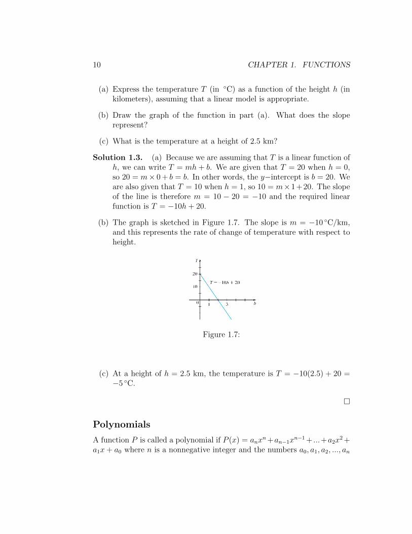
Solution 1.3. (a) Because we are assuming that T is a linear function ofh, we can write T = mh + b. We are given that T = 20 when h = 0,so 20 = m× 0 + b = b. In other words, the y−intercept is b = 20. Weare also given that T = 10 when h = 1, so 10 = m×1+20. The slopeof the line is therefore m = 10 − 20 = −10 and the required linearfunction is T = −10h+ 20.
(b) The graph is sketched in Figure 1.7. The slope is m = −10 ◦C/km,and this represents the rate of change of temperature with respect toheight.
Figure 1.7:
(c) At a height of h = 2.5 km, the temperature is T = −10(2.5) + 20 =−5 ◦C.
�
Polynomials
A function P is called a polynomial if P (x) = anxn+an−1x
n−1 + ...+a2x2 +
a1x+ a0 where n is a nonnegative integer and the numbers a0, a1, a2, ..., an
1.2. ESSENTIAL FUNCTIONS 11
are constants called the coefficients of the polynomial.
The domain of any polynomial is R = (−∞,∞). If the leading coefficientan 6= 0, then the degree of the polynomial is n. For example,
- A polynomial of degree 1 is of the form P (x) = mx+ b and so it is alinear function.
- A polynomial of degree 2 is of the form P (x) = ax2 + bx + c and iscalled a quadratic function.
- A polynomial of degree 3 is of the form P (x) = ax3 + bx2 + cx + dand is called a cubic function.
Remark 1.2.1. A polynomial of degree n has at most n zeros (roots).
Piecewise Defined Functions
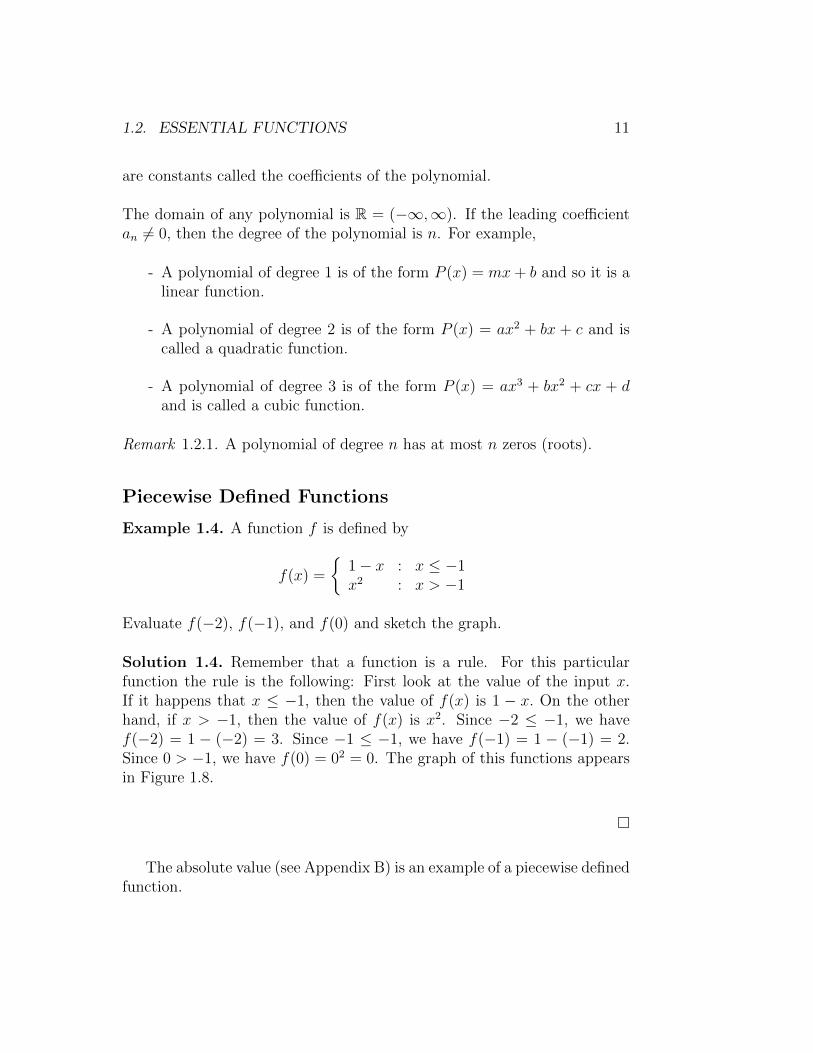
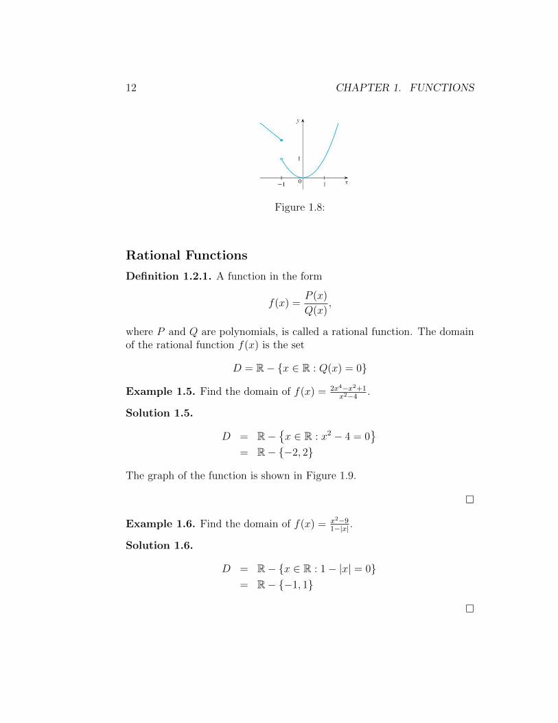
Example 1.4. A function f is defined by
f(x) =
{1− x : x ≤ −1x2 : x > −1
Evaluate f(−2), f(−1), and f(0) and sketch the graph.
Solution 1.4. Remember that a function is a rule. For this particularfunction the rule is the following: First look at the value of the input x.If it happens that x ≤ −1, then the value of f(x) is 1 − x. On the otherhand, if x > −1, then the value of f(x) is x2. Since −2 ≤ −1, we havef(−2) = 1 − (−2) = 3. Since −1 ≤ −1, we have f(−1) = 1 − (−1) = 2.Since 0 > −1, we have f(0) = 02 = 0. The graph of this functions appearsin Figure 1.8.
�
The absolute value (see Appendix B) is an example of a piecewise definedfunction.
12 CHAPTER 1. FUNCTIONS
Figure 1.8:
Rational Functions
Definition 1.2.1. A function in the form
f(x) =P (x)
Q(x),
where P and Q are polynomials, is called a rational function. The domainof the rational function f(x) is the set
D = R− {x ∈ R : Q(x) = 0}
Example 1.5. Find the domain of f(x) = 2x4−x2+1x2−4 .
Solution 1.5.
D = R−{x ∈ R : x2 − 4 = 0
}= R− {−2, 2}
The graph of the function is shown in Figure 1.9.
�
Example 1.6. Find the domain of f(x) = x2−91−|x| .
Solution 1.6.
D = R− {x ∈ R : 1− |x| = 0}= R− {−1, 1}
�

1.2. ESSENTIAL FUNCTIONS 13
Figure 1.9:
Exercise 1.1. What is the domain of each of the following functions.
(a) f(x) = 1|1−x|
(b) g(x) = −4x10+x2
Root Function
Definition 1.2.2. For any integer n ≥ 2,
f(x) = n√g(x)
is the nth root function of g(x). The domain of the root function dependson the value of n if it is even or odd.
n is odd: The domain of f(x) in this case is the same as the domain ofg(x). The range of f(x) will be R.
n is even: In this case, the domain of f(x) is the set
D = {x ∈ R : g(x) ≥ 0} ∩ {g(x) domain}
The range of f is [0,∞).
Example 1.7. Find the domain of f(x) = 3√x2 − 4.
Solution 1.7. Since f is odd root function, then
D = domain (x2 − 4) = R

14 CHAPTER 1. FUNCTIONS
Example 1.8. Find the domain of f(x) =√x2 − 4.
Solution 1.8. Since f is even root function, then
D ={x ∈ R : x2 − 4 ≥ 0
}∩ { domain of x2 − 4}
= (−∞,−2] ∪ [2,∞) ∩ R= (−∞,−2] ∪ [2,∞)
�
Example 1.9. Find the domain of f(x) = 6√|x|.
Solution 1.9. Since f is even root function, then
D = {x ∈ R : |x| ≥ 0} ∩ { domain of |x|}= R ∩ R= R
�
Example 1.10. Find the domain of f(x) = 1√9−x2 .
Solution 1.10. This function is rational and its denominator is evenroot. The root’s domain is the dominant here. The domain of f is
D ={
domain of√
9− x2}−{x ∈ R :
√9− x2 = 0
}=
{x ∈ R : 9− x2 > 0
}∩ { domain of 9− x2}
={x ∈ R : x2 < 9
}∩ R
= {x ∈ R : |x| < 3} ∩ R= (−3, 3) ∩ R= (−3, 3)
�
Example 1.11. Find the domain of f(x) = 11−√x.
1.2. ESSENTIAL FUNCTIONS 15
Solution 1.11. This example is quite different from the previous example.The function f here is rational but its denominator contains an even root.The root’s domain is also the dominant here. So, the domain of f is
D ={
domain of√x}−{x ∈ R : 1−
√x = 0
}= {x ∈ R : x ≥ 0} ∩ { domain of x} − {1}= [0,∞) ∩ R− {1}= [0,∞)− {1}= [0, 1) ∪ (1,∞)
�
Example 1.12. Find the domain of f(x) =√
2−√x.
Solution 1.12. Since f is even root function that contains an even rootfunction inside it, then both roots are dominant here. Hence, the domainof f is
D ={x ∈ R : 2−
√x ≥ 0
}∩ { domain of 2−
√x}
={x ∈ R :
√x ≤ 2
}∩ {x ∈ R : x ≥ 0} ∩ { domain of x}
= {x ∈ R : 0 ≤ x ≤ 4} ∩ [0,∞) ∩ R= [0, 4] ∩ [0,∞) ∩ R= [0, 4]
�
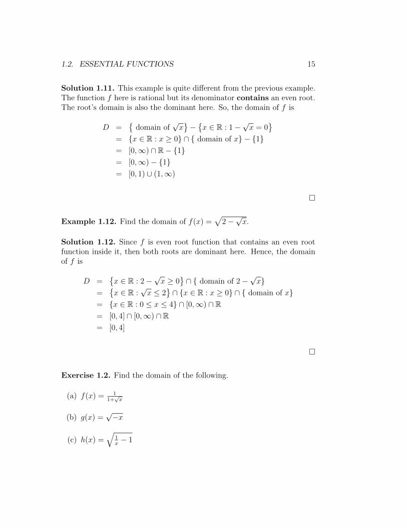
Exercise 1.2. Find the domain of the following.
(a) f(x) = 11+√x
(b) g(x) =√−x
(c) h(x) =√
1x− 1

16 CHAPTER 1. FUNCTIONS
Figure 1.10:
Trigonometric Functions
In calculus the convention is that radian measure is always used (exceptwhen otherwise indicated). Figure 1.10 shows a sector of a circle withcentral angle θ and radius r subtending an arc with length s. Then theradian measure of the central angle A′CB′ is the number θ = s
r.
Example 1.13. Find the radian measure of 60◦.
Solution 1.13. To convert degrees to radians, multiply degrees by (π rad )/180◦.
60◦ = 60( π
180
)=π
3.
�
Example 1.14. Express 5π/4 in degrees.
Solution 1.14. To convert radians to degrees, multiply radians by 180◦/(π rad ).
5π
4rad =
(5π
4
)(180◦
π
)= 225◦.
�
Nonzero radians measures can be positive or negative and can go beyond2π = 360◦. The standard position of an angle occurs when we place itsvertex at the origin of a coordinate system and its initial side on the positivex−axis as in Figure 1.11. A positive angle is obtained by rotating the initialside counterclockwise until it coincides with the terminal side. Likewise,negative angles are obtained by clockwise rotation.
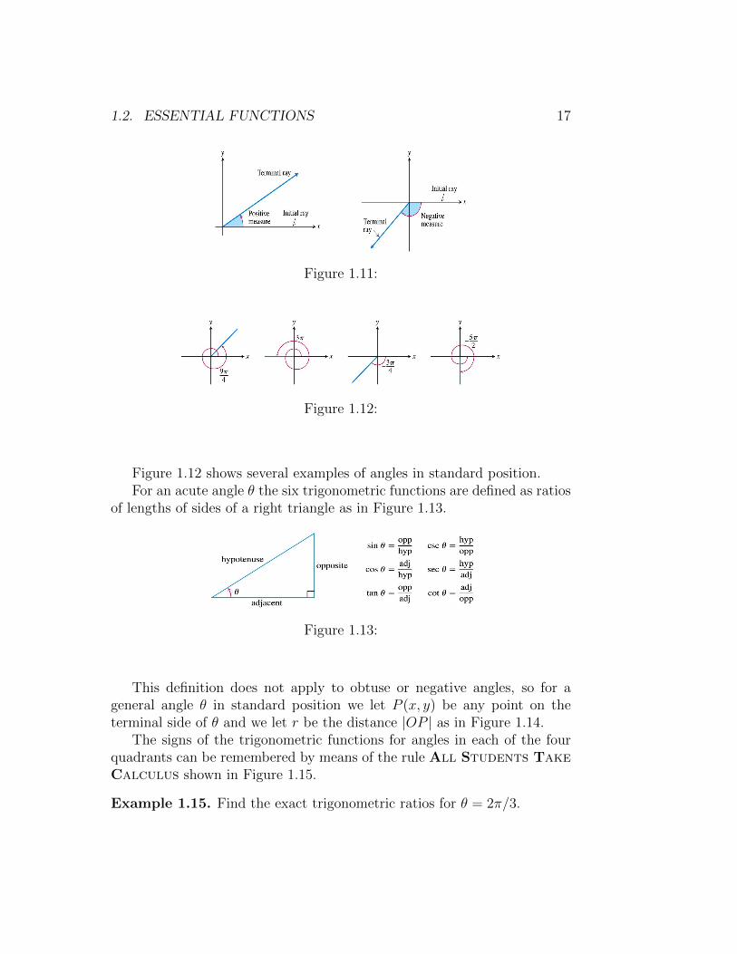
1.2. ESSENTIAL FUNCTIONS 17
Figure 1.11:
Figure 1.12:
Figure 1.12 shows several examples of angles in standard position.For an acute angle θ the six trigonometric functions are defined as ratios
of lengths of sides of a right triangle as in Figure 1.13.
Figure 1.13:
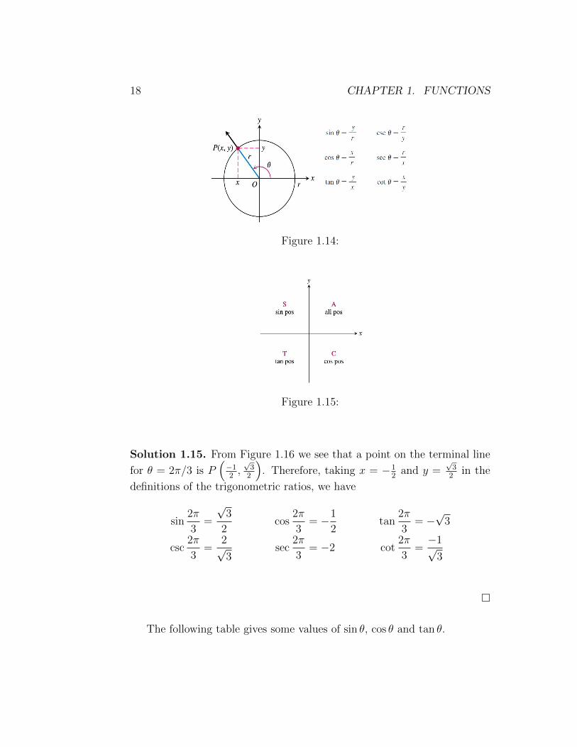
This definition does not apply to obtuse or negative angles, so for ageneral angle θ in standard position we let P (x, y) be any point on theterminal side of θ and we let r be the distance |OP | as in Figure 1.14.
The signs of the trigonometric functions for angles in each of the fourquadrants can be remembered by means of the rule All Students TakeCalculus shown in Figure 1.15.
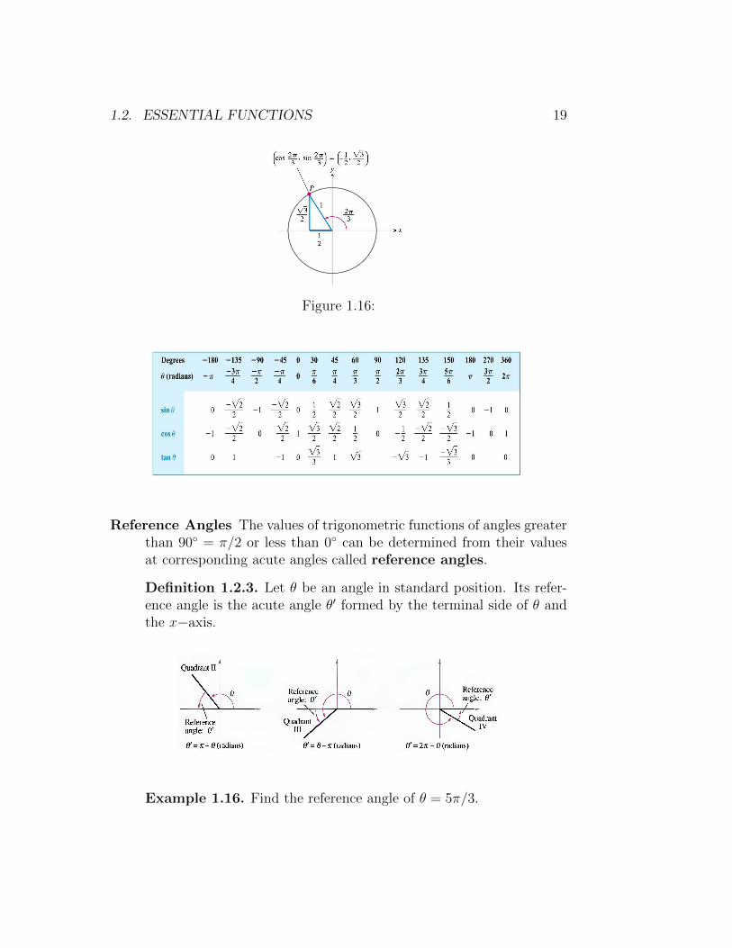
Example 1.15. Find the exact trigonometric ratios for θ = 2π/3.
18 CHAPTER 1. FUNCTIONS
Figure 1.14:
Figure 1.15:
Solution 1.15. From Figure 1.16 we see that a point on the terminal line
for θ = 2π/3 is P(−12,√32
). Therefore, taking x = −1
2and y =
√32
in the
definitions of the trigonometric ratios, we have
sin2π
3=
√3
2cos
2π
3= −1
2tan
2π
3= −√
3
csc2π
3=
2√3
sec2π
3= −2 cot
2π
3=−1√
3
�
The following table gives some values of sin θ, cos θ and tan θ.
1.2. ESSENTIAL FUNCTIONS 19
Figure 1.16:
Reference Angles The values of trigonometric functions of angles greaterthan 90◦ = π/2 or less than 0◦ can be determined from their valuesat corresponding acute angles called reference angles.
Definition 1.2.3. Let θ be an angle in standard position. Its refer-ence angle is the acute angle θ′ formed by the terminal side of θ andthe x−axis.
Example 1.16. Find the reference angle of θ = 5π/3.
20 CHAPTER 1. FUNCTIONS
Solution 1.16. Because 5π/3 = 300◦ lies in quadrant 4, the angle itmakes with the x−axis is
θ′ = 2π − 5π/3 = π/3 = 60◦.
�
Example 1.17. Find the reference angle of θ = −3π/4.
Solution 1.17. First, note that −3π/4 = 135◦ is coterminal with5π/4 = 225◦ which lies in quadrant 3. So, the reference angle is
θ′ = 5π/4− π = π/4 = 45◦.
�
Example 1.18. Evaluate each of the following.
a) cos (4π/3)
b) tan (−210◦)
c) csc (11π/4)
Solution 1.18. a) Because θ = 4π/3 = 240◦ lies in quadrant 3,the reference angle is θ′ = 4π/3−π = π/3. Moreover, the cosineis negative in quadrant 3, so
cos (4π/3) = (−) cos (π/3) = −1/2
b) Because −210◦+360◦ = 150◦, it follows that −210◦ is coterminalwith the second-quadrant angle 150◦. Therefore, the referenceangle is θ′ = 180◦ − 150◦ = 30◦. Finally, because the tangent isnegative in quadrant 2, you have
tan (−210◦) = (−) tan (30◦) = −√
3/3 = −1/√
3
c) Because 11π/4− 2π = 3π/4, it follows that 11π/4 is coterminalwith the second-quadrant angle 3π/4. Therefore, the referenceangle is θ′ = π − 3π/4 = π/4. Because the cosecant is positivein quadrant 2, you have
csc (11π/4) = (+) csc (π/4) = 1/ sin (π/4) =√
2

1.2. ESSENTIAL FUNCTIONS 21
Trigonometric Identities A trigonometric identity is a relationship amongthe trigonometric functions. The most identities are the following.
Part 1 The following identities are immediate consequences of thedefinitions of the trigonometric functions.
csc θ =1
sin θ, sec θ =
1
cos θ, cot θ =
1
tan θ
tan θ =sin θ
cos θ, cot θ =
cos θ
sin θ
Part 2 The following are the most useful of all trigonometric identi-ties:
sin2 θ + cos2 θ = 1
tan2 θ + 1 = sec2 θ
1 + cot2 θ = csc2 θ
Part 3 The following identities show that sin θ is an odd functionand cos θ is an even function.
sin(−θ) = − sin θ, cos(−θ) = cos θ
Part 4 The next identities show that the sine and cosine functionsare periodic with period 2π Since the angles θ and θ+ 2π havethe same terminal side.
sin(θ + 2π) = sin θ, cos(θ + 2π) = cos θ
Part 5 The addition and subtracting formulas are the followingidentities.
sin(x+ y) = sinx cos y + cosx sin y
sin(x− y) = sinx cos y − cosx sin y
cos(x+ y) = cosx cos y − sinx sin y
cos(x− y) = cosx cos y − sinx sin y
tan(x+ y) =tanx+ tan y
1− tanx tan y
tan(x− y) =tanx− tan y
1 + tan x tan y

22 CHAPTER 1. FUNCTIONS
Part 6 The double-angle formulas are:
sin(2x) = 2 sinx cosx
cos(2x) = cos2 x− sin2 x
cos(2x) = 2 cos2 x− 1
cos(2x) = 1− 2 sin2 x
Part 7 The following are the half-angle formulas, which are usefulin integral calculus:
cos2 x =1 + cos(2x)
2, sin2 x =
1− cos(2x)
2
Part 8 Finally, we state the product formulas, which are:
sinx cos y =1
2[sin(x+ y) + sin(x− y)]
cosx cos y =1
2[cos(x+ y) + cos(x− y)]
sinx sin y =1
2[cos(x− y)− cos(x+ y)]
There are many other trigonometric identities, but those we havestated are the ones used most often in calculus.
Graphs of Trigonometric Functions Graphs of the six basic trigono-metric functions using radian measure are shown in Figure 1.17. Theshading for each trigonometric function indicates its periodicity.
The graph of the function f(x) = sinx, shown in Figure 1.17(b), isobtained by plotting points for 0 ≤ x ≤ 2π and then using the periodicnature of the function to complete the graph. Notice that the zerosof the sine function occur at the integer multiples of π, that is,
sinx = 0 whenever x = nπ, n = 0,±1,±2,±3, · · ·
Because of the identity
cosx = sin(x+
π
2
)

1.2. ESSENTIAL FUNCTIONS 23
Figure 1.17:
the graph of cosine is obtained by shifting the graph of sine by anamount π/2 to the left [see Figure 1.17(a)]. Therefore, the zeros ofthe cosine function occur at the integer multiples of π plus π/2, thatis,
cosx = 0 whenever x =π
2+ nπ, n = 0,±1,±2,±3, · · ·
Note that for both the sine and cosine functions the domain is R =(−∞,∞) and the range is the closed interval [−1, 1]. Thus, for allvalues of x, we have
−1 ≤ sinx ≤ 1 or we write | sinx| ≤ 1
−1 ≤ cosx ≤ 1 or we write | cosx| ≤ 1
The tangent and cotangent have range R = (−∞,∞), whereas cose-cant and secant have range (−∞,−1]∪ [1,∞). All four functions are
24 CHAPTER 1. FUNCTIONS
periodic: tangent and cotangent have period π, whereas cosecant andsecant have period 2π. Since
tanx =sinx
cosx, cotx =
cosx
sinx, secx =
1
cosx, cscx =
1
sinx
then the zeros of the tangent function is the same as of the sine func-tion, and the zeros of the cotangent function is the same as of thecosine function, while the secant and cosecant functions have no ze-ros.
Example 1.19. Solve the following equations.
a) sinx = 1
b) cos x = −1
Solution 1.19. a) sinx equals 1 when x = π/2 plus multiples of2π, see Figure 1.17(b). So,
sinx = 1 whenever x =π
2+ 2nπ where n = 0,±1,±2,±3, · · ·
b) cos x equals −1 when x = π plus multiples of 2π, see Figure1.17(a). So,
cosx = 1 whenever x = π + 2nπ where n = 0,±1,±2,±3, · · ·
�
Exercise 1.3. Solve the following equations.
a) sinx = −1
b) secx = 1
c) tan x = 1
d) cos x = 1/2
e) cos(2x) = 0
Example 1.20. Find the domain of the following.
a) f(x) = 1/(1 + sin x)
1.2. ESSENTIAL FUNCTIONS 25
b) f(x) = 1/(1− 2 cosx)
c) f(x) = cscx/√
2− xd) f(x) = sin
√x
e) f(x) =√
sinx
Solution 1.20. a) Since f is rational function, then
The domain of f = R− {x ∈ R : 1 + sinx = 0}= R− {x ∈ R : sinx = −1}
= R−{x =
3π
2+ 2nπ
}where n = 0,±1,±2, · · ·
b) Note that f is also rational function. So
The domain of f = R− {x ∈ R : 1− 2 cosx = 0}
= R−{x ∈ R : cosx =
1
2
}= R−
{x =
π
3+ 2nπ or x = −π
3+ 2nπ
}where n = 0,±1,±2, · · ·
c) First, we write
f(x) =cscx√2− x
=1
sinx√
2− x.
Therefore,
The domain of f = {domain√
2− x} −{x ∈ R : sinx
√2− x = 0
}= {x ∈ R : 2− x > 0} ∩ {domain 2− x}
−{x ∈ R : sinx = 0}= (−∞, 2) ∩ R− {x = nπ}= (−∞, 2)− {x = nπ}
where n = 0,±1,±2, · · ·
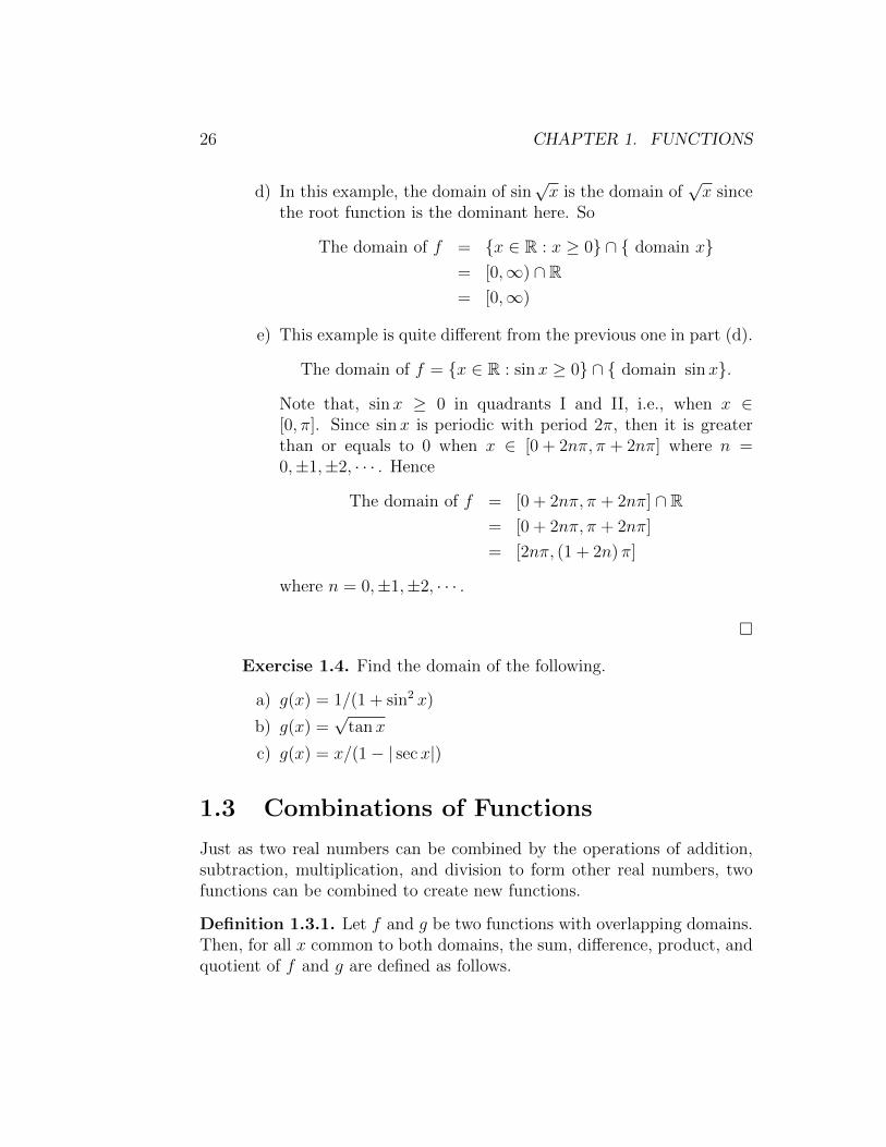
26 CHAPTER 1. FUNCTIONS
d) In this example, the domain of sin√x is the domain of
√x since
the root function is the dominant here. So
The domain of f = {x ∈ R : x ≥ 0} ∩ { domain x}= [0,∞) ∩ R= [0,∞)
e) This example is quite different from the previous one in part (d).
The domain of f = {x ∈ R : sinx ≥ 0} ∩ { domain sinx}.
Note that, sinx ≥ 0 in quadrants I and II, i.e., when x ∈[0, π]. Since sinx is periodic with period 2π, then it is greaterthan or equals to 0 when x ∈ [0 + 2nπ, π + 2nπ] where n =0,±1,±2, · · · . Hence
The domain of f = [0 + 2nπ, π + 2nπ] ∩ R= [0 + 2nπ, π + 2nπ]
= [2nπ, (1 + 2n) π]
where n = 0,±1,±2, · · · .
�
Exercise 1.4. Find the domain of the following.
a) g(x) = 1/(1 + sin2 x)
b) g(x) =√
tanx
c) g(x) = x/(1− | secx|)
1.3 Combinations of Functions
Just as two real numbers can be combined by the operations of addition,subtraction, multiplication, and division to form other real numbers, twofunctions can be combined to create new functions.
Definition 1.3.1. Let f and g be two functions with overlapping domains.Then, for all x common to both domains, the sum, difference, product, andquotient of f and g are defined as follows.
1.3. COMBINATIONS OF FUNCTIONS 27
Sum: (f + g) (x) = f (x) + g (x); x ∈ domain f ∩ domain g
Difference: (f − g) (x) = f (x)−g (x) ; x ∈ domain f∩ domain g
Product: (f × g) (x) = f (x)× g (x) ; x ∈ domain f ∩ domain g
Quotient: (f/g) (x) = f (x) /g (x) ; x ∈ domain f ∩ domain gand g(x) 6= 0.
Example 1.21. Find (f/g) (x) and (g/f) (x) for the functions given byf(x) =
√x and g(x) =
√4− x2. Then find the domains of f/g and g/f .
Solution 1.21. The quotient of f and g is(f
g
)(x) =
f(x)
g(x)=
√x√
4− x2.
The quotient of g and f is(g
f
)(x) =
g(x)
f(x)=
√4− x2√x
.
The domain of f is [0,∞) and the domain of g is [−2, 2]. The intersectionof these domains is [0, 2]. So, the domains for f/g and g/f are as follows.
Domain of (f/g) is [0, 2)
Domain of (g/f) is (0, 2]
�
Exercise 1.5. Given f(x) = 2x+ 1 and g(x) = 1x
+ 2x− 1, find (f − g)(x)and its domain. Then evaluate the difference when x = 2.
Definition 1.3.2. The composition of the function f with the function gis
(f ◦ g) (x) = f (g(x)) .
The domain of f ◦ g is the set of all x in the domain of g such that g(x) isin the domain of f (See Figure 1.18.)

28 CHAPTER 1. FUNCTIONS
Figure 1.18:
The domain of f ◦ g is the set of all x in the domain of g such that g(x)is in the domain of f . In other words, (f ◦ g)(x) is defined whenever bothg and f(g(x)) are defined.
Example 1.22. Find the domain of the composition (f ◦ g)(x) for thefunctions given by f(x) = x2 − 9 and g(x) =
√9− x2.
Solution 1.22. The composition of the functions is as follows.
(f ◦ g)(x) = f(g(x))
= f(√
9− x2)
=(√
9− x2)2− 9
=(9− x2
)− 9
= −x2
From this, it might appear that the domain of the composition is the setof all real numbers. This, however, is not true.Because the domain of −x2is the set of all real numbers and the domain of g is [−3, 3], the domain of(f ◦ g) is [−3, 3].
�

1.3. COMBINATIONS OF FUNCTIONS 29
Example 1.23. Let g(x) =√
2− x. Find g ◦ g and its domain.
Solution 1.23.
(g ◦ g)(x) = g(g(x))
= g(√
2− x)
=
√2−√
2− x
This expression is defined when both 2 − x ≥ 0 and 2 −√
2− x ≥ 0. Thefirst inequality means x ≤ 2, and the second is equivalent to
√2− x ≤ 2
2− x ≤ 4
x ≥ −2
Thus −2 ≤ x ≤ 2, so the domain of g ◦ g is the closed interval [−2, 2].
�
It is possible to take the composition of three or more functions. Forinstance, the composite function f ◦ g ◦ h is found by first applying h, theng, and then f as follows:
(f ◦ g ◦ h)(x) = f(g(h(x)))
Example 1.24. Find f ◦ g ◦ h if f(x) = x/(x + 1), g(x) = x10, andh(x) = x+ 3.
Solution 1.24.
(f ◦ g ◦ h)(x) = f(g(h(x)))
= f(g(x+ 3))
= f((x+ 3)10
)=
(x+ 3)10
(x+ 3)10 + 1
�

30 CHAPTER 1. FUNCTIONS
So far we have used composition to build complicated functions fromsimpler ones. But in calculus it is often useful to be able to decompose acomplicated function into simpler ones, as in the following example.
Example 1.25. Given F (x) = cos2(x+ 9), find functions f , g, and h suchthat F = f ◦ g ◦ h.
Solution 1.25. Since F (x) = [cos(x+ 9)]2, the formula for F says: Firstadd 9, then take the cosine of the result, and finally square. So we let
h(x) = x+ 9
g(x) = cosx
f(x) = x2
Then
(f ◦ g ◦ h)(x) = f(g(h(x)))
= f(g(x+ 9))
= f(cos(x+ 9))
= cos2(x+ 9) = F (x).
�
1.4 Inverse Functions
Remember that, a function can be represented by a set of ordered pairs.For instance, the function f(x) = x+ 4 from the set A = {1, 2, 3, 4} to theset B = {5, 6, 7, 8} can be written as follows.
f(x) = x+ 4 : {(1, 5), (2, 6), (3, 7), (4, 8)}.
In this case, by interchanging the first and second coordinates of each ofthese ordered pairs, you can form the inverse function of f , which is denotedby f−1. It is a function from the set B to the set A, and can be written asfollows.
f−1(x) = x− 4 : {(5, 1), (6, 2), (7, 3), (8, 4)}.
Note that the domain of f is equal to the range of f−1, and vice versa, asshown in Figure 1.19. Also note that the functions f and f−1 have the effect

1.4. INVERSE FUNCTIONS 31
of ”undoing” each other. In other words, when you form the compositionof f with f−1 or the composition of f−1 with f , you obtain the identityfunction.
f(f−1(x)
)= f(x− 4) = (x− 4) + 4 = x
f−1 (f(x)) = f−1(x+ 4) = (x+ 4)− 4 = x
Figure 1.19:
Definition 1.4.1. A function is called a one−to−one function if it nevertakes on the same value twice; that is,
f (x1) 6= f (x2) whenever x1 6= x2
We have the following geometric method for determining whether a func-tion is one-to-one.
Definition 1.4.2. Horizontal Line Test: A function is one-to-one if andonly if no horizontal line intersects its graph more than once.
Example 1.26. Is the function f(x) = x3 one-to-one?
Solution 1.26. If x1 6= x2, then x31 6= x32 (two different numbers cant havethe same cube). Therefore, by Definition 1.4.1, f(x) = x3 is one-to-one.From Figure 1.20 we see that no horizontal line intersects the graph off(x) = x3 more than once. Therefore, by the Horizontal Line Test, f isone-to-one.
�
Example 1.27. Is the function g(x) = x2 one-to-one?
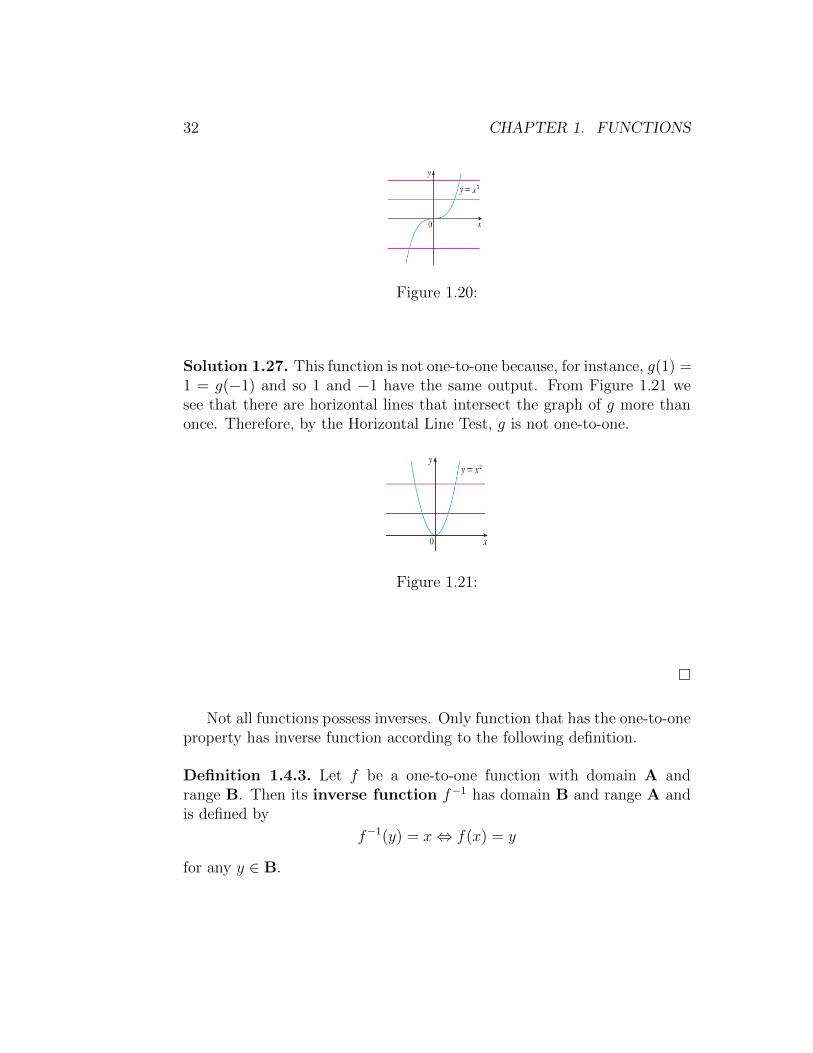
32 CHAPTER 1. FUNCTIONS
Figure 1.20:
Solution 1.27. This function is not one-to-one because, for instance, g(1) =1 = g(−1) and so 1 and −1 have the same output. From Figure 1.21 wesee that there are horizontal lines that intersect the graph of g more thanonce. Therefore, by the Horizontal Line Test, g is not one-to-one.
Figure 1.21:
�
Not all functions possess inverses. Only function that has the one-to-oneproperty has inverse function according to the following definition.
Definition 1.4.3. Let f be a one-to-one function with domain A andrange B. Then its inverse function f−1 has domain B and range A andis defined by
f−1(y) = x⇔ f(x) = y
for any y ∈ B.
1.4. INVERSE FUNCTIONS 33
Remark 1.4.1. Do not mistake the power −1 in f−1 for an exponent. Thusf−1(x) does not mean 1
f(x). The reciprocal 1
f(x)could, however, be written
as [f(x)]−1.
Remark 1.4.2. The letter x is traditionally used as the independent variable,so when we concentrate on f−1 rather than on f , we usually reverse theroles of x and y in Definition 1.4.3 and write
f−1(x) = y ⇔ f(y) = x
By this formula and Definition 1.4.3 we get the following cancelationequations:
f−1 (f (x)) = x for every x ∈ A
f(f−1 (x)
)= x for every x ∈ B
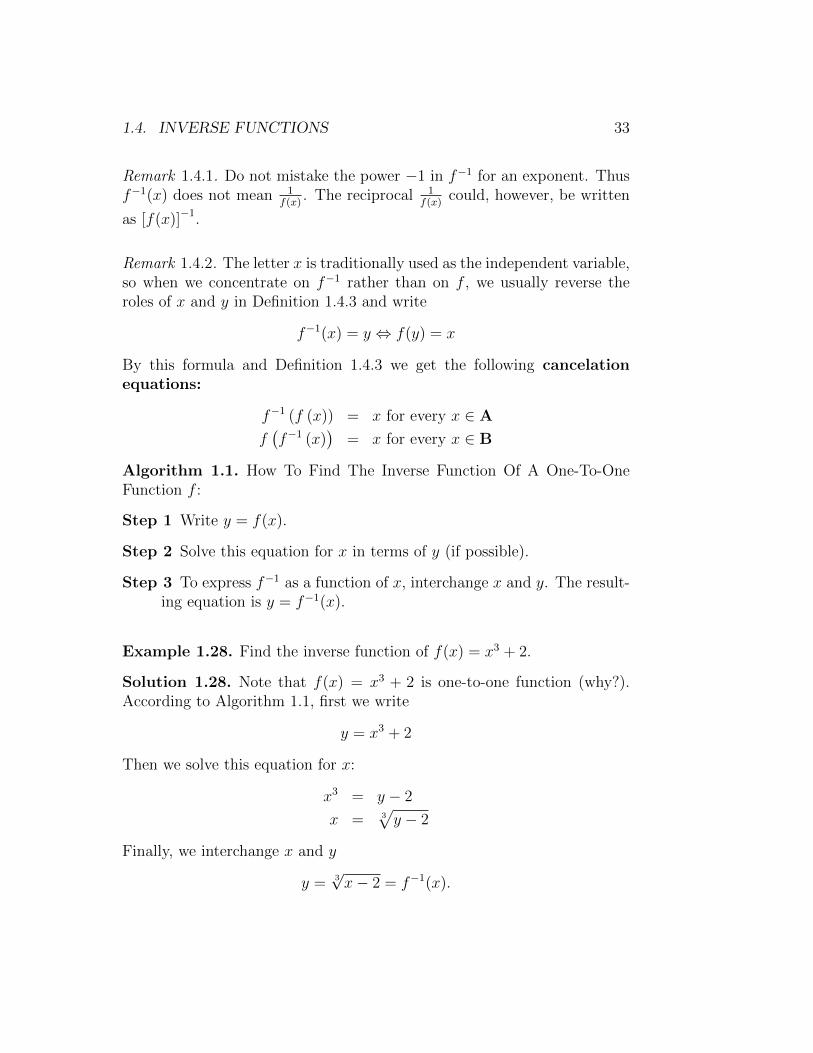
Algorithm 1.1. How To Find The Inverse Function Of A One-To-OneFunction f :
Step 1 Write y = f(x).
Step 2 Solve this equation for x in terms of y (if possible).
Step 3 To express f−1 as a function of x, interchange x and y. The result-ing equation is y = f−1(x).
Example 1.28. Find the inverse function of f(x) = x3 + 2.
Solution 1.28. Note that f(x) = x3 + 2 is one-to-one function (why?).According to Algorithm 1.1, first we write
y = x3 + 2
Then we solve this equation for x:
x3 = y − 2
x = 3√y − 2
Finally, we interchange x and y
y = 3√x− 2 = f−1(x).

34 CHAPTER 1. FUNCTIONS
Exercise 1.6. Show that f(x) = x/(x+ 1); x 6= −1 is one-to-one function,then find its inverse.
Remark 1.4.3. The graph of f−1 is obtained by reflecting the graph of fabout the line y = x as illustrated by Figure 1.22.
Figure 1.22:
Inverse Trigonometric Functions
When we try to find the inverse trigonometric functions, we have a slightdifficulty: Because the trigonometric functions are not one-to-one, they donot have inverse functions. The difficulty is overcome by restricting thedomains of these functions so that they become one-to-one.
You can see from Figure 1.23 that the sine function is not one-to-one (usethe Horizontal Line Test). But the function f(x) = sin x, −π/2 ≤ x ≤ π/2,is one-to-one (see Figure 1.23). The inverse function of this restricted sinefunction exists and is denoted by sin−1 or arcsin. It is called the inversesine function or the arcsine function.
The following table summarizes the definitions of the three most com-mon inverse trigonometric functions.
Function Domain Rangey = sin−1 x↔ sin y = x x ∈ [−1, 1] y ∈
[−π
2, π2
]y = cos−1 x↔ cos y = x x ∈ [−1, 1] y ∈ [0, π]y = tan−1 x↔ tan y = x x ∈ R y ∈
(−π
2, π2
)

1.4. INVERSE FUNCTIONS 35
Figure 1.23:
Exercise 1.7. Find the domain of f(x) = sin−1 (x2 − 4)
Example 1.29. If possible, find the exact value of
1. sin−1(−1
2
)2. sin−1
(√32
)3. sin−1 (2)
4. cos−1(√
22
)5. cos−1 (−1)
6. tan−1 (0)
7. tan−1 (1)
Solution 1.29. 1. Because sin(−π
6
)= −1
2and −π
6∈[−π
2, π2
], it follows
that sin−1(−1
2
)= −π
6.
2. Because sin(π3
)=√32
and π3∈[−π
2, π2
], it follows that sin−1
(√32
)=
π3.
3. It is not possible to evaluate y = sin−1 x at x = 2 because there is noangle whose sine is 2. Remember that the domain of the inverse sinefunction is [−1, 1].
4. Because cos(π4
)=√22
and π4∈ [0, π], it follows that cos−1
(√22
)= π
4.

36 CHAPTER 1. FUNCTIONS
5. Because cos (π) = −1 and π ∈ [0, π], it follows that cos−1 (−1) = π.
6. Because tan (0) = 0 and 0 ∈(−π
2, π2
), it follows that tan−1 (0) = 0.
7. Because tan(−π
4
)= −1 and−π
4∈(−π
2, π2
), it follows that tan−1 (−1) =
−π4.
�
The following are some important identities of inverse trigonometricfunctions.
1. sin−1 (−x) = − sin−1 (x) for all x ∈ [−1, 1]
2. tan−1 (−x) = − tan−1 (x) for all x ∈ R
3. cos−1 (−x) = π − cos−1 (x) for all x ∈ [−1, 1]
4. sin−1 (x) + cos−1 (x) = π2
for all x ∈ [−1, 1]
5. sin(sin−1 x
)= x for all x ∈ [−1, 1], and sin−1 (sinx) = x for all
x ∈[−π
2, π2
]6. cos (cos−1 x) = x for all x ∈ [−1, 1], and cos−1 (cosx) = x for allx ∈ [0, π]
7. tan (tan−1 x) = x for all x ∈ R, and tan−1 (tanx) = x for all x ∈(−π
2, π2
)8. sin−1 (sinx) =
{π − x : π
2≤ x ≤ 3π
2
x− 2nπ : x ≥ 3π2
where n = 0,±1,±2, · · · .
9. cos−1 (cosx) = 2nπ − x if x ≥ π where n = 0,±1,±2, · · · .
10. cos(sin−1 x
)= sin (cos−1 x) =
√1− x2 for all x ∈ [−1, 1].
11. tan(sin−1 x
)= x√
1−x2 for all x ∈ [−1, 1].
Example 1.30. If possible, find the exact value of
1. tan (tan−1 (−5))
1.4. INVERSE FUNCTIONS 37
2. sin−1(sin(5π3
))3. cos (cos−1 (π))
4. cos−1(cos(17π4
))5. tan
(cos−1
(23
))6. cos
(sin−1
(−3
5
))Solution 1.30. 1. Because −5 ∈ R , the inverse property applies, and
you have tan (tan−1 (−5)) = −5.
2. In this case, 5π3
does not lie within the range of the arcsine function[−π
2, π2
]. However, 5π
3is coterminal with 5π
3− 2π = −π
3∈[−π
2, π2
],
and you have
sin−1(
sin
(5π
3
))= sin−1
(sin(−π
3
))= −π
3
3. The expression cos (cos−1 (π)) is not defined because cos−1 (π) is notdefined. Remember that the domain of the inverse cosine function is[−1, 1].
4. In this case, 17π4
does not lie within the range of the cosine function[0, π]. However, 17π
4is coterminal with 2(2)π − 17π
4= −π
4, and you
have
cos−1(
cos
(17π
4
))= cos−1
(cos(−π
4
))= cos−1
(cos(π
4
))=π
4
5. If you let u = cos−1(23
)then cosu = 2
3. Because cosu is positive, u is
a first-quadrant angle. You can sketch and label angle u as shown inFigure 1.24. Consequently
tan
(cos−1
(2
3
))= tanu =
opp
adj=
√5
2.
38 CHAPTER 1. FUNCTIONS
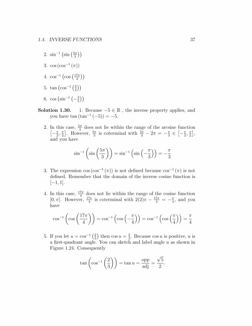
Figure 1.24:
6. If you let u = sin−1(−3
5
)then sinu = 3
5. Because sinu is negative,
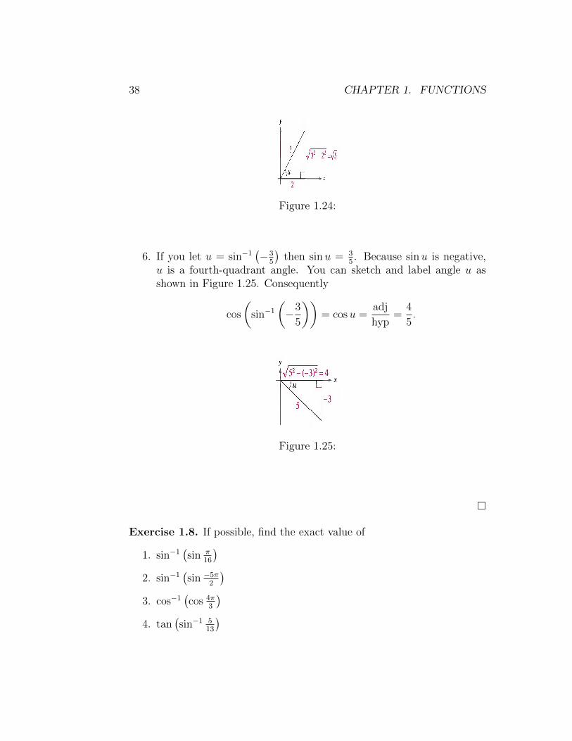
u is a fourth-quadrant angle. You can sketch and label angle u asshown in Figure 1.25. Consequently
cos
(sin−1
(−3
5
))= cosu =
adj
hyp=
4
5.
Figure 1.25:
�
Exercise 1.8. If possible, find the exact value of
1. sin−1(sin π
16
)2. sin−1
(sin −5π
2
)3. cos−1
(cos 4π
3
)4. tan
(sin−1 5
13
)
1.4. INVERSE FUNCTIONS 39
5. sec(sin−1 3
4
)6. cos (tan−1 2)
7. sin(2 cos−1 3
5
)Exponential and Logarithmic Functions
In this part you will study two types of non−algebraic functions: exponen-tial functions and logarithmic functions. These functions are examples oftranscendental functions.
Definition 1.4.4. The exponential function f with base a is denoted byf(x) = ax where a > 0, a 6= 1, and x is any real number. The domain ofthe exponential function f(x) = ag(x) is the same as the domain of g(x).
Note that in the definition of an exponential function, the base a = 1is excluded because it yields f(x) = 1x = 1. This is a constant function,not an exponential function. You already know how to evaluate ax forinteger and rational values of x. For example, you know that 43 = 64 and41/2 =
√4 = 2.
The exponential function f(x) = ax, a > 0, a 6= 1 is different from all thefunctions you have studied so far because the variable x is an exponent. Adistinguishing characteristic of an exponential function is its rapid increaseas x increases (for a > 1). Many real-life phenomena with patterns of rapidgrowth (or decline) can be modeled by exponential functions. The basiccharacteristics of the exponential function are summarized below in Figure1.26.
Figure 1.26:
40 CHAPTER 1. FUNCTIONS
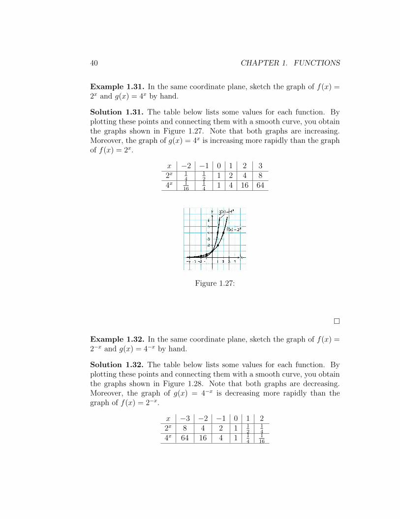
Example 1.31. In the same coordinate plane, sketch the graph of f(x) =2x and g(x) = 4x by hand.
Solution 1.31. The table below lists some values for each function. Byplotting these points and connecting them with a smooth curve, you obtainthe graphs shown in Figure 1.27. Note that both graphs are increasing.Moreover, the graph of g(x) = 4x is increasing more rapidly than the graphof f(x) = 2x.
x −2 −1 0 1 2 32x 1
412
1 2 4 84x 1
1614
1 4 16 64
Figure 1.27:
�
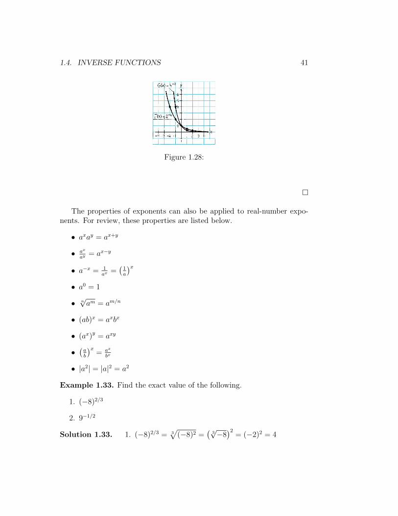
Example 1.32. In the same coordinate plane, sketch the graph of f(x) =2−x and g(x) = 4−x by hand.
Solution 1.32. The table below lists some values for each function. Byplotting these points and connecting them with a smooth curve, you obtainthe graphs shown in Figure 1.28. Note that both graphs are decreasing.Moreover, the graph of g(x) = 4−x is decreasing more rapidly than thegraph of f(x) = 2−x.
x −3 −2 −1 0 1 22x 8 4 2 1 1
214
4x 64 16 4 1 14
116
1.4. INVERSE FUNCTIONS 41
Figure 1.28:
�
The properties of exponents can also be applied to real-number expo-nents. For review, these properties are listed below.
• axay = ax+y
• ax
ay= ax−y
• a−x = 1ax
=(1a
)x• a0 = 1
• n√am = am/n
• (ab)x = axbx
• (ax)y = axy
•(ab
)x= ax
bx
• |a2| = |a|2 = a2
Example 1.33. Find the exact value of the following.
1. (−8)2/3
2. 9−1/2
Solution 1.33. 1. (−8)2/3 = 3√
(−8)2 =(
3√−8)2
= (−2)2 = 4

42 CHAPTER 1. FUNCTIONS
2. 9−1/2 = 191/2
=(19
)1/2=√
19
= 13
�
The Natural Base e: For many applications, the convenient choice for abase is the irrational number e ≈ 2.7182. This number is called thenatural base. The function f(x) = ex is called the natural exponen-tial function and its graph is shown in Figure 1.29. The graph of theexponential function has the same basic characteristics as the graphof the function f(x) = ax. Be sure you see that for the exponentialfunction f(x) = ex, e is the constant 2.7182, whereas x is the variable.
Figure 1.29:
The number e can be approximated by the expression(1 +
1
x
)xfor large values of x.
We learned that if a function is one-to-one-that is, if the function hasthe property such that no horizontal line intersects its graph more thanonce-the function must have an inverse function. By looking back at thegraphs of the exponential functions introduced in Figure 1.26, you will seethat every function of the form
f(x) = ax, a > 0, a 6= 1
passes the Horizontal Line Test and therefore must have an inverse func-tion. This inverse function is called the logarithmic function with basea.
1.4. INVERSE FUNCTIONS 43
Definition 1.4.5. For x > 0, a > 0, and a 6= 1,
y = loga x if and only if x = ay.
The function given by f(x) = loga x (read as log base a of x) is called thelogarithmic function with base a. The domain of the logarithmic functionf(x) = loga g(x) is
{x ∈ R : g(x) > 0} ∩ the domain of g(x)
The equations y = loga x and x = ay are equivalent. The first equa-tion is in logarithmic form and the second is in exponential form. Whenevaluating logarithms, remember that a logarithm is an exponent. Thismeans that loga x is the exponent to which a must be raised to obtain x.For instance, logz 8 = 3 because 2 must be raised to the third power to get 8.
Example 1.34. Use the definition of logarithmic function to evaluate eachlogarithm at the indicated value of x.
1. f(x) = log2 x, at x = 32
2. f(x) = log3 x, at x = 1
3. f(x) = log4 x, at x = 2
4. f(x) = log10 x, at x = 1100
Solution 1.34. 1. f(32) = log2 32 = 5 because 25 = 32
2. f(1) = log3 1 = 0 because 30 = 1
3. f(2) = log4 2 = 12
because 412 =√
4 = 2
4. f(
1100
)= log10
1100
= −2 because 10−2 = 1102
= 1100
�
The following properties follow directly from the definition of the loga-rithmic function with base a.
44 CHAPTER 1. FUNCTIONS
1. loga 1 = 0 because a0 = 1
2. loga a = 1 because a1 = a
3. loga bx = x loga b
4. loga ax = x and aloga x = x
5. loga(x× y) = loga x+ loga y
6. loga(x÷ y) = loga x− loga y
7. If loga x = loga y, then x = y
Example 1.35. Find the exact value of the following.
1. log2 16
2. log9 3
3. 5−2 log5 2
4. log10 0.001
5. log6 9− log6 5 + log6 20
Solution 1.35. 1. log2 16 = log2 24 = 4 log2 2 = 4× 1 = 4
2. log9 3 = log9 912 = 1
2log9 9 = 1
2× 1 = 1
2
3. 5−2 log5 2 = 5log5 2−2
= 2−2 = 122
= 14
4. log10 0.001 = log101
1000= log10
1103
= log10 10−3 = −3 log10 10 = −3×1 = −3
5. log6 9−log6 5+log6 20 = log6
(95
)+log6 20 = log6
(95× 20
)= log6 36 =
log6 62 = 2 log6 6 = 2× 1 = 2
�
1.4. INVERSE FUNCTIONS 45
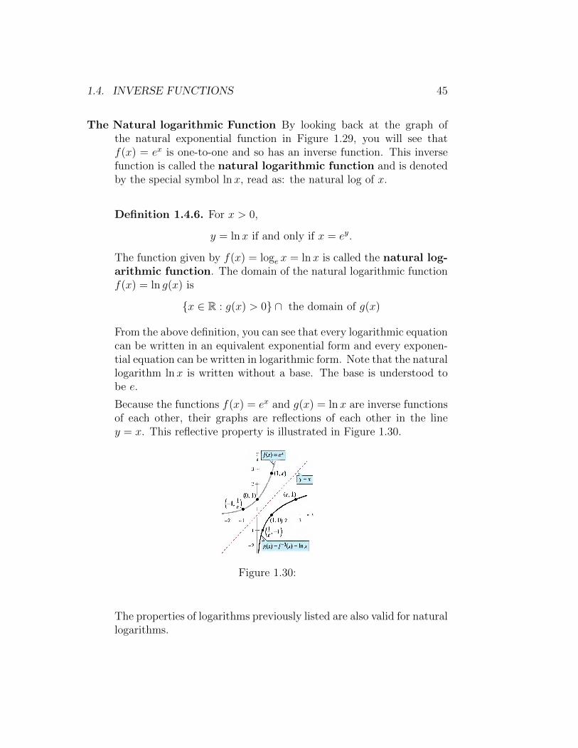
The Natural logarithmic Function By looking back at the graph ofthe natural exponential function in Figure 1.29, you will see thatf(x) = ex is one-to-one and so has an inverse function. This inversefunction is called the natural logarithmic function and is denotedby the special symbol lnx, read as: the natural log of x.
Definition 1.4.6. For x > 0,
y = lnx if and only if x = ey.
The function given by f(x) = loge x = lnx is called the natural log-arithmic function. The domain of the natural logarithmic functionf(x) = ln g(x) is
{x ∈ R : g(x) > 0} ∩ the domain of g(x)
From the above definition, you can see that every logarithmic equationcan be written in an equivalent exponential form and every exponen-tial equation can be written in logarithmic form. Note that the naturallogarithm lnx is written without a base. The base is understood tobe e.
Because the functions f(x) = ex and g(x) = ln x are inverse functionsof each other, their graphs are reflections of each other in the liney = x. This reflective property is illustrated in Figure 1.30.
Figure 1.30:
The properties of logarithms previously listed are also valid for naturallogarithms.
46 CHAPTER 1. FUNCTIONS
1. ln 1 = 0 because e0 = 1
2. ln e = 1 because e1 = e
3. ln ax = x ln a
4. ln ex = x and elnx = x
5. ln(x× y) = lnx+ ln y
6. ln(x÷ y) = lnx− ln y
7. If lnx = ln y, then x = y
8. loga b = ln b/ ln a
Exercise 1.9. Find the exact value of (log2 3) (log3 4) (log4 5) · · · (log31 32).
So far in this part, you have studied the definitions, graphs, and prop-erties of exponential and logarithmic functions. Now, you will study proce-dures for solving equations involving exponential and logarithmic functions.There are two basic strategies for solving exponential or logarithmic equa-tions. The first is based on the One-to-One Properties and the second isbased on the Inverse Properties.
For a > 0 and a 6= l, the following properties are true for all x and y forwhich loga x and loga y are defined.
One-to-One Properties ax = ay if and only if x = y, and loga x = loga yif and only if x = y.
Inverse Properties aloga x = x and loga ax = x.
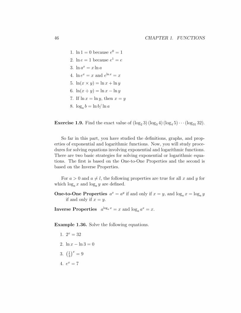
Example 1.36. Solve the following equations.
1. 2x = 32
2. lnx− ln 3 = 0
3.(13
)x= 9
4. ex = 7
1.4. INVERSE FUNCTIONS 47
5. ln x = −3
6. log10 x = −1
Solution 1.36.
Original Equation Rewritten Equation Solution Property2x = 32 2x = 25 x = 5 One-to-Onelnx− ln 3 = 0 lnx = ln 3 x = 3 One-to-One(13
)x= 9 3−x = 32 x = −2 One-to-One
ex = 7 ln ex = ln 7 x = ln 7 Inverselnx = −3 elnx = e−3 x = e−3 Inverselog10 x = −1 10log10 x = 10−1 x = 10−1 = 1
10Inverse
�
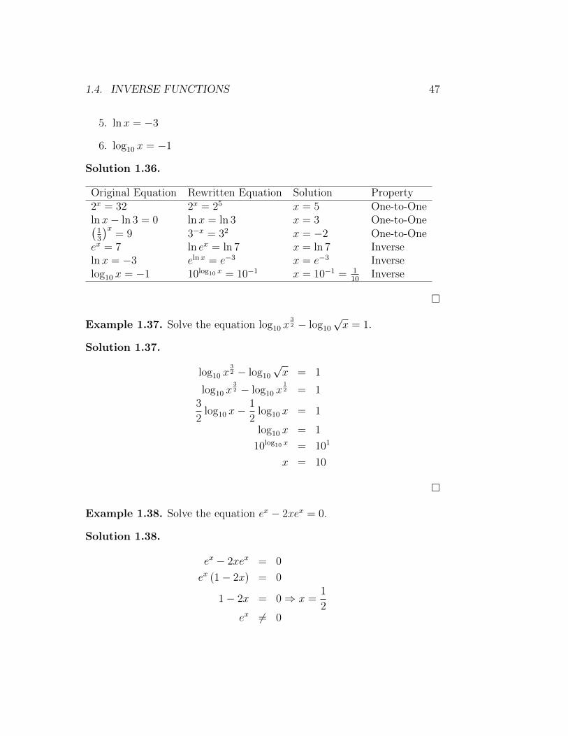
Example 1.37. Solve the equation log10 x32 − log10
√x = 1.
Solution 1.37.
log10 x32 − log10
√x = 1
log10 x32 − log10 x
12 = 1
3
2log10 x−
1
2log10 x = 1
log10 x = 1
10log10 x = 101
x = 10
�
Example 1.38. Solve the equation ex − 2xex = 0.
Solution 1.38.
ex − 2xex = 0
ex (1− 2x) = 0
1− 2x = 0⇒ x =1
2ex 6= 0
48 CHAPTER 1. FUNCTIONS
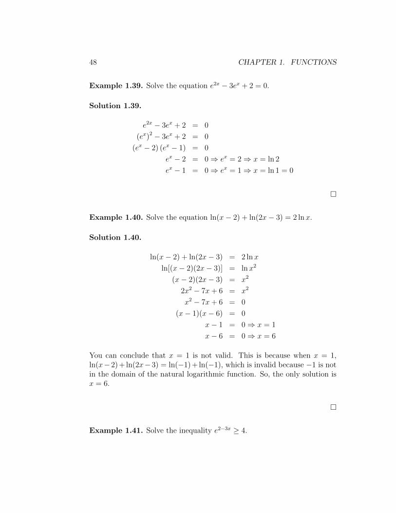
Example 1.39. Solve the equation e2x − 3ex + 2 = 0.
Solution 1.39.
e2x − 3ex + 2 = 0
(ex)2 − 3ex + 2 = 0
(ex − 2) (ex − 1) = 0
ex − 2 = 0⇒ ex = 2⇒ x = ln 2
ex − 1 = 0⇒ ex = 1⇒ x = ln 1 = 0
�
Example 1.40. Solve the equation ln(x− 2) + ln(2x− 3) = 2 lnx.
Solution 1.40.
ln(x− 2) + ln(2x− 3) = 2 lnx
ln[(x− 2)(2x− 3)] = lnx2
(x− 2)(2x− 3) = x2
2x2 − 7x+ 6 = x2
x2 − 7x+ 6 = 0
(x− 1)(x− 6) = 0
x− 1 = 0⇒ x = 1
x− 6 = 0⇒ x = 6
You can conclude that x = 1 is not valid. This is because when x = 1,ln(x− 2) + ln(2x− 3) = ln(−1) + ln(−1), which is invalid because −1 is notin the domain of the natural logarithmic function. So, the only solution isx = 6.
�
Example 1.41. Solve the inequality e2−3x ≥ 4.
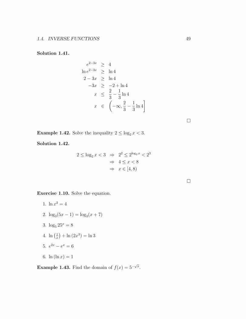
1.4. INVERSE FUNCTIONS 49
Solution 1.41.
e2−3x ≥ 4
ln e2−3x ≥ ln 4
2− 3x ≥ ln 4
−3x ≥ −2 + ln 4
x ≤ 2
3− 1
3ln 4
x ∈(−∞, 2
3− 1
3ln 4
]�
Example 1.42. Solve the inequality 2 ≤ log2 x < 3.
Solution 1.42.
2 ≤ log2 x < 3 ⇒ 22 ≤ 2log2 x < 23
⇒ 4 ≤ x < 8
⇒ x ∈ [4, 8)
�
Exercise 1.10. Solve the equation.
1. ln x2 = 4
2. log3(5x− 1) = log3(x+ 7)
3. log5 25x = 8
4. ln(1x
)+ ln (2x3) = ln 3
5. e2x − ex = 6
6. ln (lnx) = 1
Example 1.43. Find the domain of f(x) = 5−√x.
50 CHAPTER 1. FUNCTIONS
Solution 1.43.
The domain of 5−√x = The domain of
√x
= {x ∈ R : x ≥ 0} ∩ The domain of x
= [0,∞) ∩ R= [0,∞)
�
Example 1.44. Find the domain of f(x) = 1− e 1x .
Solution 1.44.
The domain of 1− e1x = The domain of
1
x= R− {x ∈ R : x = 0}= R− {0}
�
Example 1.45. Find the domain of f(x) =√ex.
Solution 1.45.
The domain of√ex = {x ∈ R : ex ≥ 0} ∩ The domain of ex
= R ∩ R= R
�
Example 1.46. Find the domain of f(x) = ln x2.
Solution 1.46.
The domain of lnx2 = {x ∈ R : x2 > 0} ∩ The domain of x2
= (R− {0}) ∩ R= R− {0}
�

1.4. INVERSE FUNCTIONS 51
Example 1.47. Find the domain of f(x) = 2 lnx.
Solution 1.47.
The domain of 2 lnx = {x ∈ R : x > 0} ∩ The domain of x
= (0,∞) ∩ R= (0,∞)
�
Example 1.48. Find the domain of f(x) = log4 (9− 16x2).
Solution 1.48.
The domain of log4
(9− 16x2
)=
{x ∈ R : 9− 16x2 > 0
}∩Domain of 9− 16x2
=
{x ∈ R : x2 <
9
16
}∩ R
=
{x ∈ R :
√x2 <
√9
16
}∩ R
=
{x ∈ R : |x| < 3
4
}∩ R
=
{x ∈ R : −3
4< x <
3
4
}∩ R
=
(−3
4,3
4
)∩ R
=
(−3
4,3
4
)�
Example 1.49. Find the domain of f(x) = log3(1−√x).
Solution 1.49.
The domain of log3(1−√x) =
{x ∈ R : 1−
√x > 0
}∩ The domain of
√x
={x ∈ R :
√x < 1
}∩ {x ∈ R : x ≥ 0} ∩ R
= {x ∈ R : 0 ≤ x < 1} ∩ [0,∞) ∩ R= [0, 1) ∩ [0,∞) ∩ R= [0, 1)
52 CHAPTER 1. FUNCTIONS
Exercise 1.11. Find the domain of the following.
1. f(x) = e4+x2
2. f(x) = ln cosx
3. f(x) = log10 (1− ex)
4. f(x) = 11−ex
5. f(x) = ln (1 + ln x)
6. f(x) =√
2− 2x
7. f(x) = ln(4− x)
Example 1.50. Find a formula for the inverse of the function.
1. f(x) = e2x−1
2. f(x) = ln(x+ 3)
Solution 1.50. 1. First, let y = e2x−1. By inverse property we haveln y = ln e2x−1 and then ln y = 2x − 1. So, x = (1 + ln y)/2. Hence,f−1(x) = (1 + lnx)/2.
2. Let y = ln(x+ 3). By inverse property we have ey = eln(x+3) and theney = x+ 3. So, x = ey − 3. Hence, f−1(x) = ex − 3.
�
Exercise 1.12. Find a formula for the inverse of the function.
1. g(t) = 32t−1
2. g(t) = log10(t+ 3)
1.5. HYPERBOLIC FUNCTIONS 53
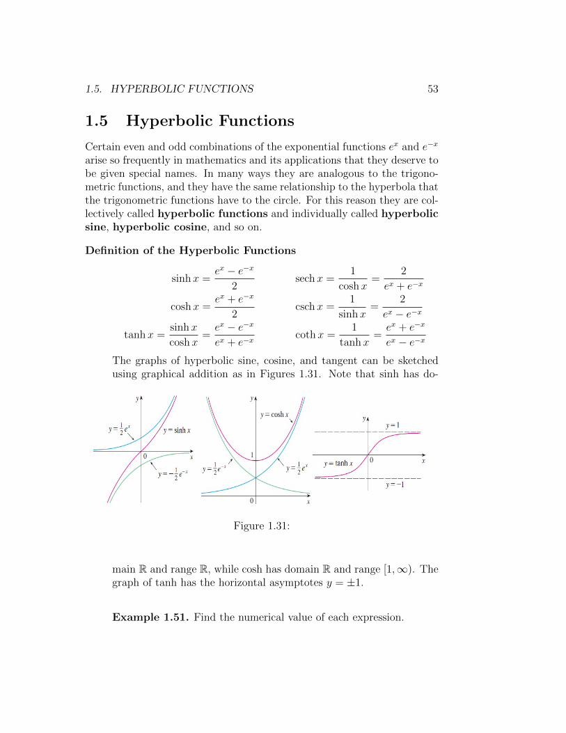
1.5 Hyperbolic Functions
Certain even and odd combinations of the exponential functions ex and e−x
arise so frequently in mathematics and its applications that they deserve tobe given special names. In many ways they are analogous to the trigono-metric functions, and they have the same relationship to the hyperbola thatthe trigonometric functions have to the circle. For this reason they are col-lectively called hyperbolic functions and individually called hyperbolicsine, hyperbolic cosine, and so on.
Definition of the Hyperbolic Functions
sinhx =ex − e−x
2sechx =
1
coshx=
2
ex + e−x
coshx =ex + e−x
2cschx =
1
sinhx=
2
ex − e−x
tanhx =sinhx
coshx=ex − e−x
ex + e−xcothx =
1
tanhx=ex + e−x
ex − e−x
The graphs of hyperbolic sine, cosine, and tangent can be sketchedusing graphical addition as in Figures 1.31. Note that sinh has do-
Figure 1.31:
main R and range R, while cosh has domain R and range [1,∞). Thegraph of tanh has the horizontal asymptotes y = ±1.
Example 1.51. Find the numerical value of each expression.

54 CHAPTER 1. FUNCTIONS
1. sinh 0
2. cosh(ln 3)
3. tanh 1
Solution 1.51. 1. sinh 0 = (e0 − e0) /2 = 0
2. cosh(ln 3) =(eln 3 + e− ln 3
)/2 = (3 + 1/3)/2 = 5/3
3. tanh 1 = (e1 − e−1) / (e1 + e−1) = (e2 − 1) / (e2 + 1)
�
Exercise 1.13. Find the numerical value of each expression.
1. cosh 0
2. sinh(ln 2)
3. sech 0
Exercise 1.14. If tanh x = 1213
, find the values of the other hyperbolicfunctions at x.
Hyperbolic Identities The hyperbolic functions satisfy a number of iden-tities that are similar to well-known trigonometric identities. We listsome of them here.
1. sinh(−x) = − sinh(x)
2. cosh(−x) = cosh(x)
3. cosh2 x− sinh2 x = 1
4. coshx+ sinhx = ex
5. coshx− sinhx = e−x
6. sinh(2x) = 2 sinhx coshx
7. cosh(2x) = sinh2 x+ cosh2 x
8. (sinhx+ coshx)n = sinh(nx) + cosh(nx) where n ∈ R9. 1− tanh2 x = sech2x
10. coth2x− 1 = csch2x
11. sinh(x+ y) = sinh x cosh y + sinh y coshx
12. cosh(x+ y) = cosh x cosh y + sinhx sinh y

1.5. HYPERBOLIC FUNCTIONS 55
13. tanh(x+ y) =tanhx+ tanh y
1 + tanh x tanh y
14. tanh(lnx) =x2 − 1
x2 + 1
15.1 + tanhx
1− tanhx= e2x
Example 1.52. Prove the identity cosh2 x− sinh2 x = 1.
Solution 1.52.
cosh2 x− sinh2 x = 1 =
(ex + e−x
2
)2
−(ex − e−x
2
)2
=e2x + 2 + e−2x
4− e2x − 2 + e−2x
4
=4
4= 1
�
Exercise 1.15. If coshx = 53
and x > 0, find the values of the otherhyperbolic functions at x.
Inverse Hyperbolic Functions You can see from Figure 1.31 that sinhand tanh are one-to-one functions and so they have inverse functionsdenoted by sinh−1 and tanh−1. Also, Figure 1.31 shows that cosh isnot one-to-one, but when restricted to the domain [0,∞) it becomesone-to-one. The inverse hyperbolic cosine function is defined as theinverse of this restricted function.
Since the hyperbolic functions are defined in terms of exponentialfunctions, its not surprising to learn that the inverse hyperbolic func-tions can be expressed in terms of logarithms. In particular, we have:
sinh−1 x = ln(x+√x2 + 1
)x ∈ R
cosh−1 x = ln(x+√x2 − 1
)x ≥ 1
tanh−1 x =1
2ln
(1 + x
1− x
)− 1 < x < 1
56 CHAPTER 1. FUNCTIONS
Example 1.53. Show that sinh−1 x = ln(x+√x2 + 1
).
Solution 1.53. Let y = sinh−1 x. Then x = sinh y = (ey − e−y) /2,so ey− 2x− e−y = 0, or, multiplying by ey, we get e2y− 2xey− 1 = 0.This is really a quadratic equation in ey:
(ey)2 − 2x (ey)− 1 = 0
Solving by the quadratic formula, we get
ey =2x±
√4x2 + 4
2= x±
√x2 + 1
Note that ey > 0, but x −√x2 + 1 < 0 (because x <
√x2 + 1).
Thus the minus sign is inadmissible and we have ey = x +√x2 + 1.
Therefore,
y = ln (ey) = ln(x+√x2 + 1
)�
Example 1.54. Find the numerical value of each expression.
1. cosh−1 1
2. sinh−1 1
Solution 1.54. 1. cosh−1 1 = ln(1 +√
12 − 1)
= ln 1 = 0
2. sinh−1 1 = ln(1 +√
12 + 1)
= ln(1 +√
2)
�
Chapter 2
Limits and Continuity
2.1 An Introduction to Limits
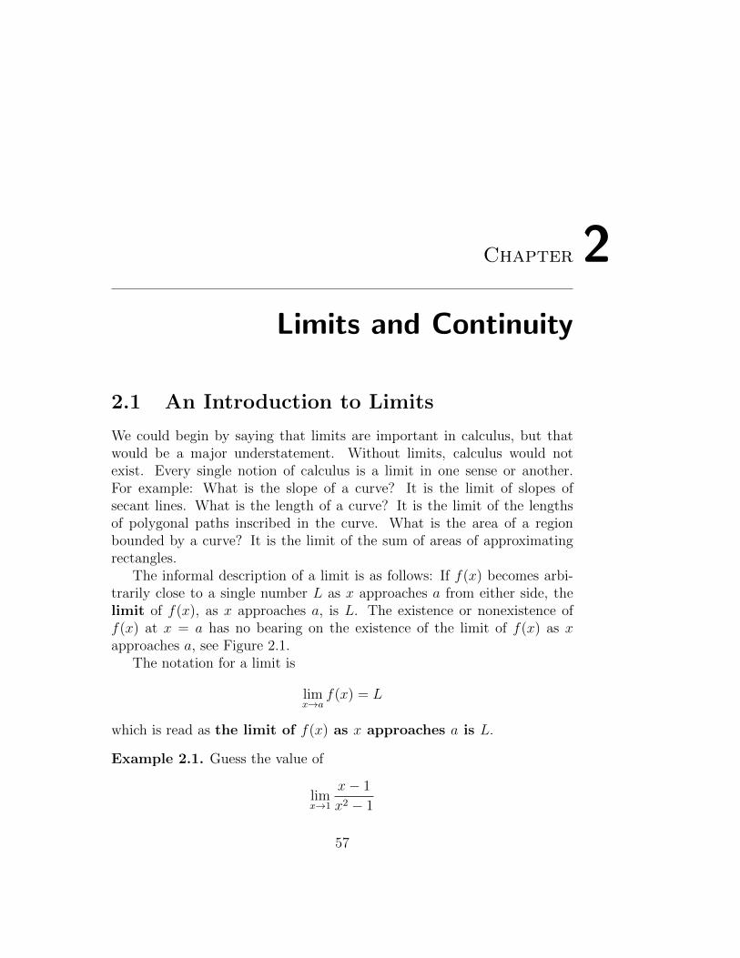
We could begin by saying that limits are important in calculus, but thatwould be a major understatement. Without limits, calculus would notexist. Every single notion of calculus is a limit in one sense or another.For example: What is the slope of a curve? It is the limit of slopes ofsecant lines. What is the length of a curve? It is the limit of the lengthsof polygonal paths inscribed in the curve. What is the area of a regionbounded by a curve? It is the limit of the sum of areas of approximatingrectangles.
The informal description of a limit is as follows: If f(x) becomes arbi-trarily close to a single number L as x approaches a from either side, thelimit of f(x), as x approaches a, is L. The existence or nonexistence off(x) at x = a has no bearing on the existence of the limit of f(x) as xapproaches a, see Figure 2.1.
The notation for a limit is
limx→a
f(x) = L
which is read as the limit of f(x) as x approaches a is L.
Example 2.1. Guess the value of
limx→1
x− 1
x2 − 1
57

58 CHAPTER 2. LIMITS AND CONTINUITY
Figure 2.1:
Solution 2.1. Notice that the function f(x) = x−1x2−1 is not defined when
x = 1, but that does not matter because the definition of limx→a f(x) saysthat we consider values of x that are close to a but not equal to a.
The table below gives values of f(x) (correct to six decimal places) forvalues of x that approach 1 (but are not equal to 1). On the basis of thevalues in the table, we make the guess that
limx→1
x− 1
x2 − 1=
1
2
x < 1 f(x) x > 1 f(x)0.5 0.666667 1.5 0.4000000.9 0.526316 1.1 0.4761900.99 0.502513 1.01 0.4975120.999 0.500250 1.001 0.4997500.9999 0.500025 1.0001 0.499975
�
Definition 2.1.1. We write
limx→a−
f(x) = L
and say the left-hand limit of f(x) as x approaches a [or the limit of f(x)as x approaches a from the left] is equal to L if we can make the values off(x) arbitrarily close to L by taking x to be sufficiently close to a and xless than a. Similarly, if we require that x be greater than a, we get theright-hand limit of f(x) as x approaches a is equal to L, and we write
limx→a+
f(x) = L
2.1. AN INTRODUCTION TO LIMITS 59
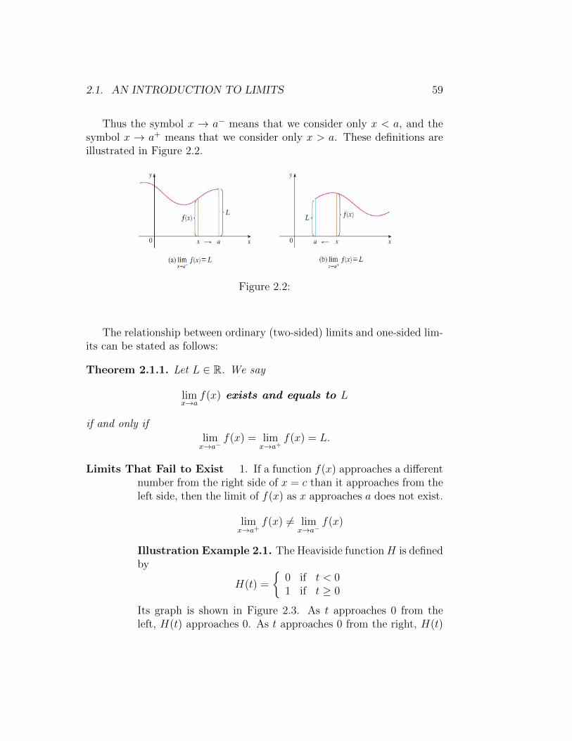
Thus the symbol x → a− means that we consider only x < a, and thesymbol x → a+ means that we consider only x > a. These definitions areillustrated in Figure 2.2.
Figure 2.2:
The relationship between ordinary (two-sided) limits and one-sided lim-its can be stated as follows:
Theorem 2.1.1. Let L ∈ R. We say
limx→a
f(x) exists and equals to L
if and only if
limx→a−
f(x) = limx→a+
f(x) = L.
Limits That Fail to Exist 1. If a function f(x) approaches a differentnumber from the right side of x = c than it approaches from theleft side, then the limit of f(x) as x approaches a does not exist.
limx→a+
f(x) 6= limx→a−
f(x)
Illustration Example 2.1. The Heaviside functionH is definedby
H(t) =
{0 if t < 01 if t ≥ 0
Its graph is shown in Figure 2.3. As t approaches 0 from theleft, H(t) approaches 0. As t approaches 0 from the right, H(t)

60 CHAPTER 2. LIMITS AND CONTINUITY
approaches 1. There is no single number that H(t) approachesas t approaches 0. Therefore,
limt→0
H(t) does not exist.
Figure 2.3:
�
2. If f(x) is not approaching a real number L−that is, if f(x) in-creases or decreases without bound−as x approaches a, you canconclude that the limit does not exist.
limx→a
f(x) =∞ or limx→a
f(x) = −∞
Illustration Example 2.2. As x becomes close to 0, x2 alsobecomes close to 0, and 1
x2becomes very large. (See the table
below.) In fact, it appears from the graph of the function f(x) =1x2
shown in Figure 2.4 that the values of f(x) can be madearbitrarily large by taking x close enough to 0. Thus the valuesof f(x) do not approach a number, so
limx→0
1
x2does not exist.
2.1. AN INTRODUCTION TO LIMITS 61
Figure 2.4:
x 1/x2
±1 1±0.5 4±0.2 25±0.1 100±0.05 400±0.01 10000±0.001 1000000
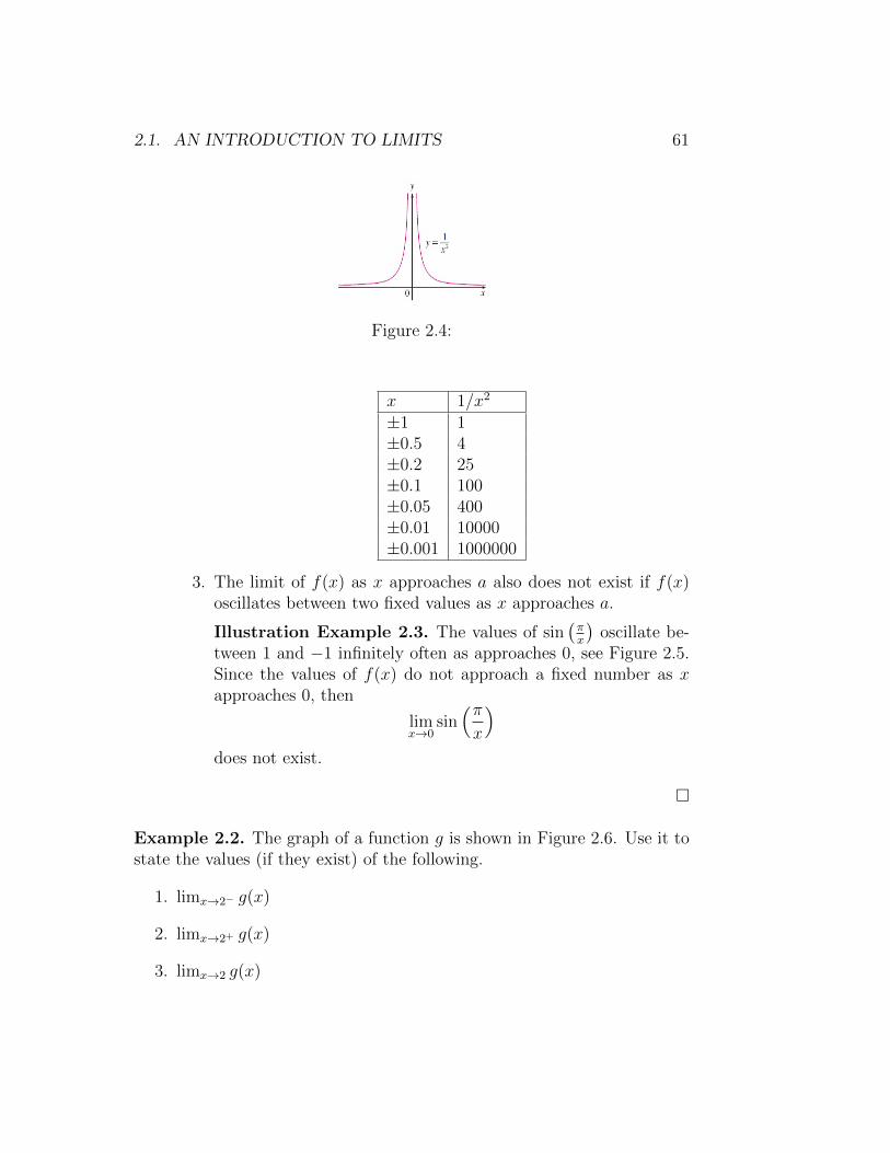
3. The limit of f(x) as x approaches a also does not exist if f(x)oscillates between two fixed values as x approaches a.
Illustration Example 2.3. The values of sin(πx
)oscillate be-
tween 1 and −1 infinitely often as approaches 0, see Figure 2.5.Since the values of f(x) do not approach a fixed number as xapproaches 0, then
limx→0
sin(πx
)does not exist.
�
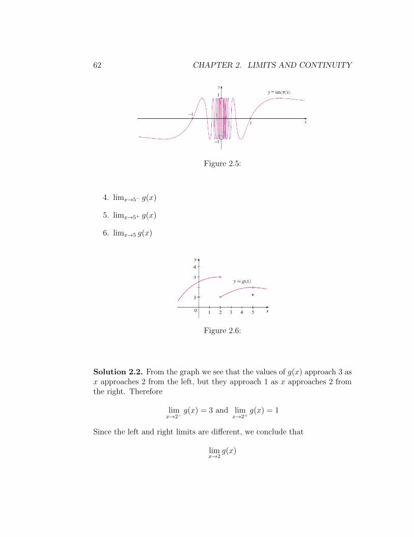
Example 2.2. The graph of a function g is shown in Figure 2.6. Use it tostate the values (if they exist) of the following.
1. limx→2− g(x)
2. limx→2+ g(x)
3. limx→2 g(x)
62 CHAPTER 2. LIMITS AND CONTINUITY
Figure 2.5:
4. limx→5− g(x)
5. limx→5+ g(x)
6. limx→5 g(x)
Figure 2.6:
Solution 2.2. From the graph we see that the values of g(x) approach 3 asx approaches 2 from the left, but they approach 1 as x approaches 2 fromthe right. Therefore
limx→2−
g(x) = 3 and limx→2+
g(x) = 1
Since the left and right limits are different, we conclude that
limx→2
g(x)
2.1. AN INTRODUCTION TO LIMITS 63
does not exist. The graph also shows that
limx→5−
g(x) = 2 and limx→5+
g(x) = 2
This time the left and right limits are the same and so, we have
limx→5
g(x) = 2.
Despite this fact, notice that g(5) 6= 2.
�
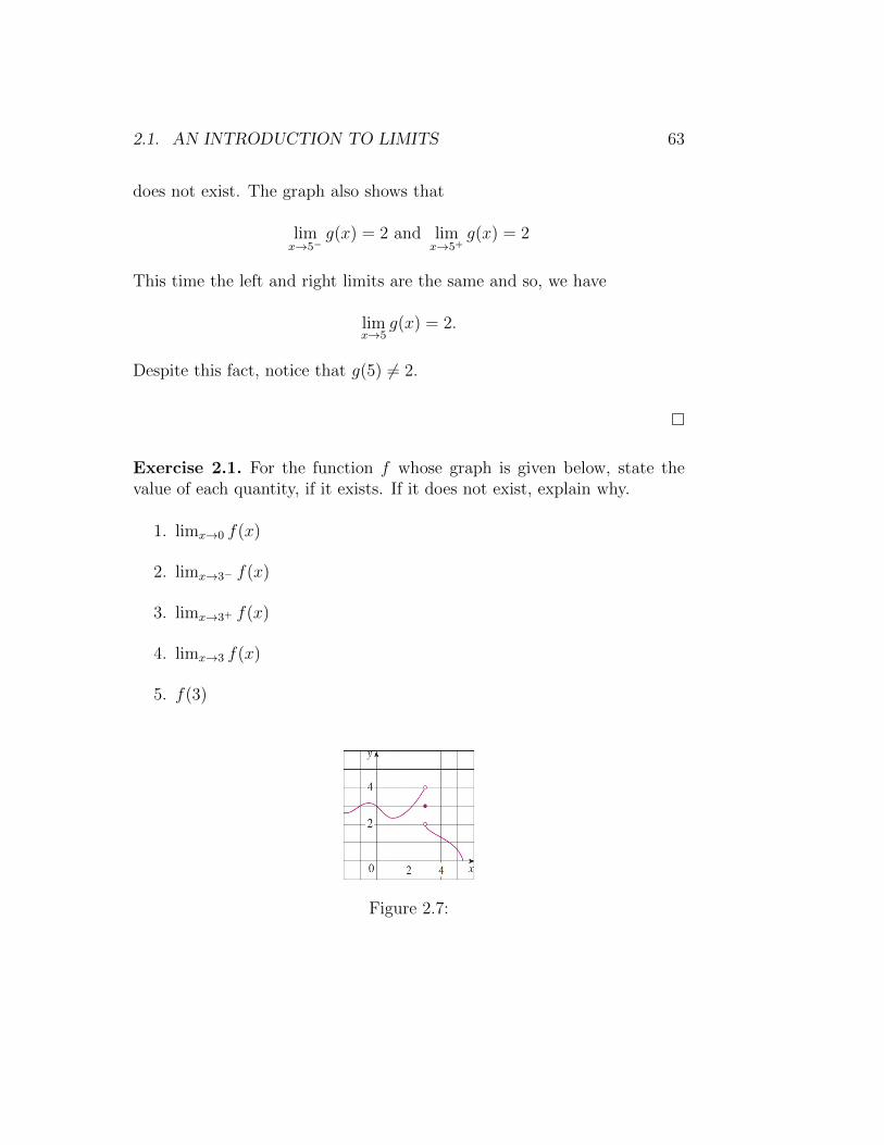
Exercise 2.1. For the function f whose graph is given below, state thevalue of each quantity, if it exists. If it does not exist, explain why.
1. limx→0 f(x)
2. limx→3− f(x)
3. limx→3+ f(x)
4. limx→3 f(x)
5. f(3)
Figure 2.7:

64 CHAPTER 2. LIMITS AND CONTINUITY
2.2 Calculating Limits using the Limit
Laws
In this section we use the following properties of limits, called the LimitLaws, to calculate limits.
Theorem 2.2.1. Suppose that c is a constant and the limits limx→a f(x)and limx→a g(x) exist. Then
1. limx→a [f(x) + g(x)] = limx→a f(x) + limx→a g(x)
2. limx→a [f(x)− g(x)] = limx→a f(x)− limx→a g(x)
3. limx→a [cf(x)] = c limx→a f(x)
4. limx→a [f(x)× g(x)] = limx→a f(x)× limx→a g(x)
5. limx→a
[f(x)g(x)
]= limx→a f(x)
limx→a g(x)if limx→a g(x) 6= 0
6. limx→a [f(x)]n = [limx→a f(x)]n where n is a positive integer.
7. limx→a c = c
8. limx→a x = a
9. limx→a xn = an where n is a positive integer.
10. limx→an√x = n
√a where n is a positive integer, and if n is even, we
assume that a > 0.
11. limx→an√f(x) = n
√limx→a f(x) where n is a positive integer, and if
n is even, we assume that limx→a f(x) > 0.
Example 2.3. Given that
limx→0.5
f(x) = 2 and limx→0.5
g(x) = −1
find
limx→0.5
[f(x)− 2g(x)]

2.2. CALCULATING LIMITS USING THE LIMIT LAWS 65
Solution 2.3.
limx→0.5
[f(x)− 2g(x)] = limx→0.5
f(x)− limx→0.5
[2g(x)]
= limx→0.5
f(x)− 2 limx→0.5
[g(x)]
= 2− 2(−1) = 4
�
Example 2.4. Evaluate
limx→−2
x3 + 2x2 − 1
5− 3x
Solution 2.4.
limx→−2
x3 + 2x2 − 1
5− 3x=
limx→−2 (x3 + 2x2 − 1)
limx→−2 (5− 3x)
=limx→−2 (x3) + limx→−2 (2x2)− limx→−2(1)
limx→−2(5)− limx→−2(3x)
=(−2)3 + 2(−2)2 − 1
5− 3(−2)
= = − 1
11
Note that if we let f(x) = x3+2x2−15−3x , then f(−2) = − 1
11. In other words, we
would have gotten the correct answer by directly substituting −2 for x.
�
Remark 2.2.1. Direct Substitution Property: If f is a polynomial or arational function and a is in the domain of f , then
limx→a
f(x) = f(a)
For example,
limx→1
(x7 − 3x5 + 1
)19=[17 − 3
(15)
+ 1]19
= (−1)19 = −1
66 CHAPTER 2. LIMITS AND CONTINUITY
because f(x) = (x7 − 3x5 + 1)19
is a polynomial whose domain is R and1 ∈ R.
Functions with the Direct Substitution Property are called continuousat a and will be studied in Section 2.5. However, not all limits can beevaluated by direct substitution. The next examples show various waysalgebraic manipulations can be used to evaluate limx→a f(x) in situationswhere f(a) is undefined. This usually happens when f(x) is a fraction withdenominator equal to 0 at x = a. Note, each of these limits involves afraction whose numerator and denominator are both 0 at the point wherethe limit is taken.
Example 2.5. Evaluate
limx→3
x2 − 9
x− 3
Solution 2.5. Let f(x) = x2−9x−3 . We can not find the limit by substituting
x = 3 because f(3) is not defined. Nor can we apply the Quotient Law,because the limit of the denominator is 0. Instead, we need to do somepreliminary algebra. We factor the numerator as a difference of squares:
(x− 3)(x+ 3)
x− 3
The numerator and denominator have a common factor of x− 3. When wetake the limit as approaches 3, we have x 6= 3 and so x− 3 6= 0. Thereforewe can cancel the common factor and compute the limit as follows:
limx→3
x2 − 9
x− 3= lim
x→3
(x− 3)(x+ 3)
x− 3= lim
x→3(x+ 3) = 6
�
Exercise 2.2. Evaluate the limit, if it exists.
1. limx→−2x2+3x+2x3+8
2. limx→−1x2+2x+1x4−1
2.2. CALCULATING LIMITS USING THE LIMIT LAWS 67
Example 2.6. Find
limt→0
√t2 + 9− 3
t2
Solution 2.6. We can not apply the Quotient Law immediately, since thelimit of the denominator is 0. Here the preliminary algebra consists ofrationalizing the numerator:
limt→0
√t2 + 9− 3
t2= lim
t→0
√t2 + 9− 3
t2·√t2 + 9 + 3√t2 + 9 + 3
= limt→0
(t2 + 9)− 9
t2(√
t2 + 9 + 3)
= limt→0
t2
t2(√
t2 + 9 + 3)
= limt→0
1√t2 + 9 + 3
=1
6
�
Exercise 2.3. Evaluate the limit, if it exists.
1. limx→164−√x
16x−x2
2. limx→8x−83√x−2
Example 2.7. Find
limx→1
√x− 1
3√x− 1
Solution 2.7. We can not apply the Quotient Law immediately, since thelimit of the denominator is 0. Here the preliminary algebra consists ofrationalizing both the numerator and the denominator by multiplying
√x+ 1√x+ 1
·3√x2 + 3
√x+ 1
3√x2 + 3
√x+ 1
68 CHAPTER 2. LIMITS AND CONTINUITY
which takes long time in calculations. The Substitution method is muchbetter in this example. The idea is: write the problem using other variabley so that the problem will transform to nice form that can easily solve. So,let
x = y6 where 6 = LCM(2, 3)
Also, as x→ 1 we have y → 6√
1 = 1. Hence,
limx→1
√x− 1
3√x− 1
= limy→1
√y6 − 1
3√y6 − 1
= limy→1
y3 − 1
y2 − 1
= limy→1
(y − 1)(y2 + y + 1)
(y − 1)(y + 1)
= limy→1
y2 + y + 1
y + 1
=3
2
�
Exercise 2.4. Evaluate
limt→0
e2t − 1
et − 1
Example 2.8. Find
limx→−4
14
+ 1x
x+ 4
Solution 2.8. We can not apply the Quotient Law immediately, since thelimit of the denominator is 0. Here the preliminary algebra consists ofsimplifying the numerator:
limx→−4
14
+ 1x
x+ 4= lim
x→−4
(1
4+
1
x
)÷ (x+ 4)
= limx→−4
x+ 4
4x· 1
x+ 4
= limx→−4
1
4x
= − 1
16
2.2. CALCULATING LIMITS USING THE LIMIT LAWS 69
Exercise 2.5. Evaluate
limt→0
(1
t√
1 + t− 1
t
)
A function f may be defined on both sides of x = a but still not have alimit at x = a. The following example shows that even if f(x) is defined atx = a, the limit of f(x) as x approaches a may not be equal to f(a).
Example 2.9. Find limx→1 g(x) where
g(x) =
{x+ 1 if x 6= 1π if x = 1
Solution 2.9. Here g is defined at x = 1 and g(1) = π, but the value ofa limit as approaches 1 does not depend on the value of the function at 1.Since g(x) = x+ 1 for x 6= 1, we have
limx→1
g(x) = limx→1
(x+ 1) = 2
�
Some limits are best calculated by first finding the left− and right−handlimits as shown in the following examples.
Example 2.10. If
f(x) =
{ √x− 4 if x > 4
8− 2x if x < 4
determine whether limx→4 f(x) exists.
Solution 2.10. Since f(x) =√x− 4 for x > 4, we have
limx→4+
f(x) = limx→4+
√x− 4 =
√4− 4 = 0
Since f(x) = 8− 2x for x < 4, we have
limx→4−
f(x) = limx→4−
(8− 2x) = 8− 2× 4 = 0
The right− and left−hand limits are equal. Thus the limit exists and
limx→4
f(x) = 0

70 CHAPTER 2. LIMITS AND CONTINUITY
Example 2.11. If
f(x) =|x− 2|
x2 + x− 6
find: limx→2+ f(x), limx→2− f(x), and limx→2 f(x)
Solution 2.11. Observe that
|x− 2| ={
x− 2 if x ≥ 2−(x− 2) if x < 2
Therefore,
limx→2+
|x− 2|x2 + x− 6
= limx→2+
x− 2
(x+ 3)(x− 2)
= limx→2+
1
x+ 3
=1
5
limx→2−
|x− 2|x2 + x− 6
= limx→2−
−(x− 2)
(x+ 3)(x− 2)
= limx→2−
−1
x+ 3
= −1
5
Since limx→2+ f(x) 6= limx→2− f(x), then the limit limx→2 f(x) does notexist.
�
Exercise 2.6. Let
f(x) =x2 − 1
|x− 1|
find: limx→1+ f(x), limx→1− f(x), and limx→1 f(x)
Example 2.12. Let g(x) =√
1− x2 find limx→1 g(x).
2.2. CALCULATING LIMITS USING THE LIMIT LAWS 71
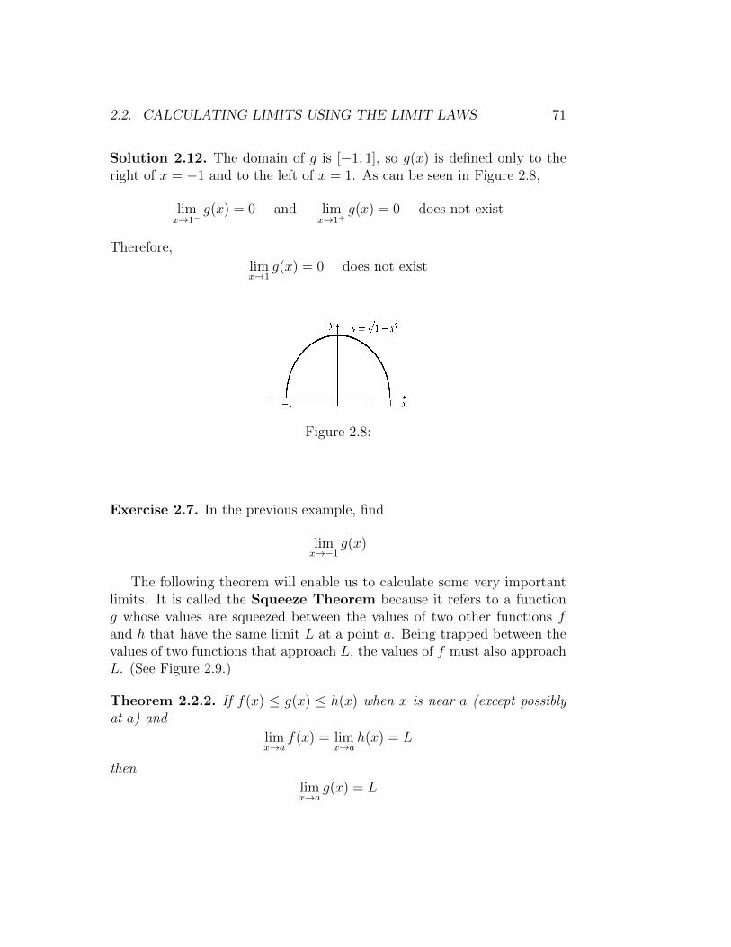
Solution 2.12. The domain of g is [−1, 1], so g(x) is defined only to theright of x = −1 and to the left of x = 1. As can be seen in Figure 2.8,
limx→1−
g(x) = 0 and limx→1+
g(x) = 0 does not exist
Therefore,
limx→1
g(x) = 0 does not exist
Figure 2.8:
Exercise 2.7. In the previous example, find
limx→−1
g(x)
The following theorem will enable us to calculate some very importantlimits. It is called the Squeeze Theorem because it refers to a functiong whose values are squeezed between the values of two other functions fand h that have the same limit L at a point a. Being trapped between thevalues of two functions that approach L, the values of f must also approachL. (See Figure 2.9.)
Theorem 2.2.2. If f(x) ≤ g(x) ≤ h(x) when x is near a (except possiblyat a) and
limx→a
f(x) = limx→a
h(x) = L
then
limx→a
g(x) = L

72 CHAPTER 2. LIMITS AND CONTINUITY
Figure 2.9:
Example 2.13. Show that
limx→0
x2 sin1
x= 0
Solution 2.13. First note that we cannot use
limx→0
x2 sin1
x= lim
x→0x2 · lim
x→0sin
1
x
because limx→0 sin 1x
does not exist. However, since
−1 ≤ sin1
x≤ 1
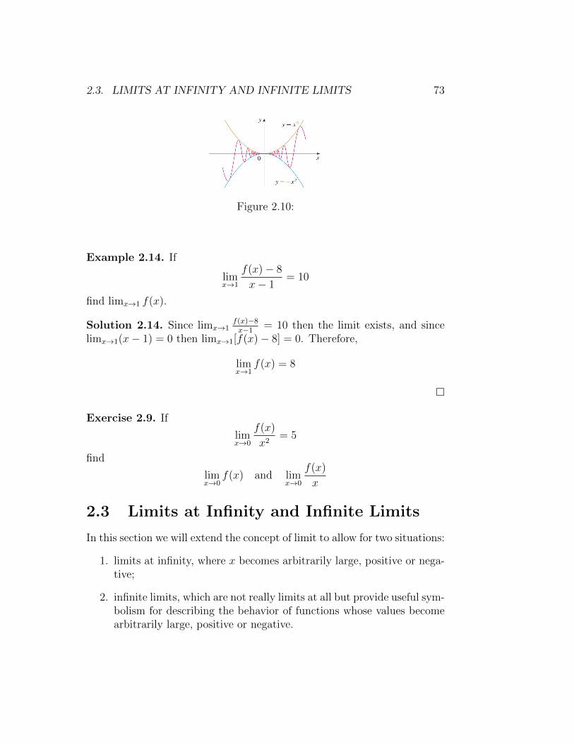
we have, as illustrated by Figure 2.10,
−x2 ≤ sin1
x≤ x2
We know thatlimx→0
x2 = 0 and limx→0
(−x2
)= 0
Taking f(x) = −x2, g(x) = x2 sin 1x, and h(x) = x2 in the Squeezing
Theorem, we obtain
limx→0
x2 sin1
x= 0
�
Exercise 2.8. If 4x− 9 ≤ f(x) ≤ x2 − 4x+ 7 for x ≥ 0, find
limx→4
f(x)
2.3. LIMITS AT INFINITY AND INFINITE LIMITS 73
Figure 2.10:
Example 2.14. If
limx→1
f(x)− 8
x− 1= 10
find limx→1 f(x).
Solution 2.14. Since limx→1f(x)−8x−1 = 10 then the limit exists, and since
limx→1(x− 1) = 0 then limx→1[f(x)− 8] = 0. Therefore,
limx→1
f(x) = 8
�
Exercise 2.9. If
limx→0
f(x)
x2= 5
find
limx→0
f(x) and limx→0
f(x)
x
2.3 Limits at Infinity and Infinite Limits
In this section we will extend the concept of limit to allow for two situations:
1. limits at infinity, where x becomes arbitrarily large, positive or nega-tive;
2. infinite limits, which are not really limits at all but provide useful sym-bolism for describing the behavior of functions whose values becomearbitrarily large, positive or negative.
74 CHAPTER 2. LIMITS AND CONTINUITY
Definition 2.3.1. If the function f is defined on an interval (a,∞) and ifwe can ensure that f(x) is as close as we want to the number L by taking xlarge enough, then we say that f(x) approaches the limit L as x approachesinfinity, and we write
limx→∞
f(x) = L
If the function f is defined on an interval (−∞, b) and if we can ensure thatf(x) is as close as we want to the number M by taking x negative and largeenough, then we say that f(x) approaches the limit M as x approachesnegative infinity, and we write
limx→−∞
f(x) = M
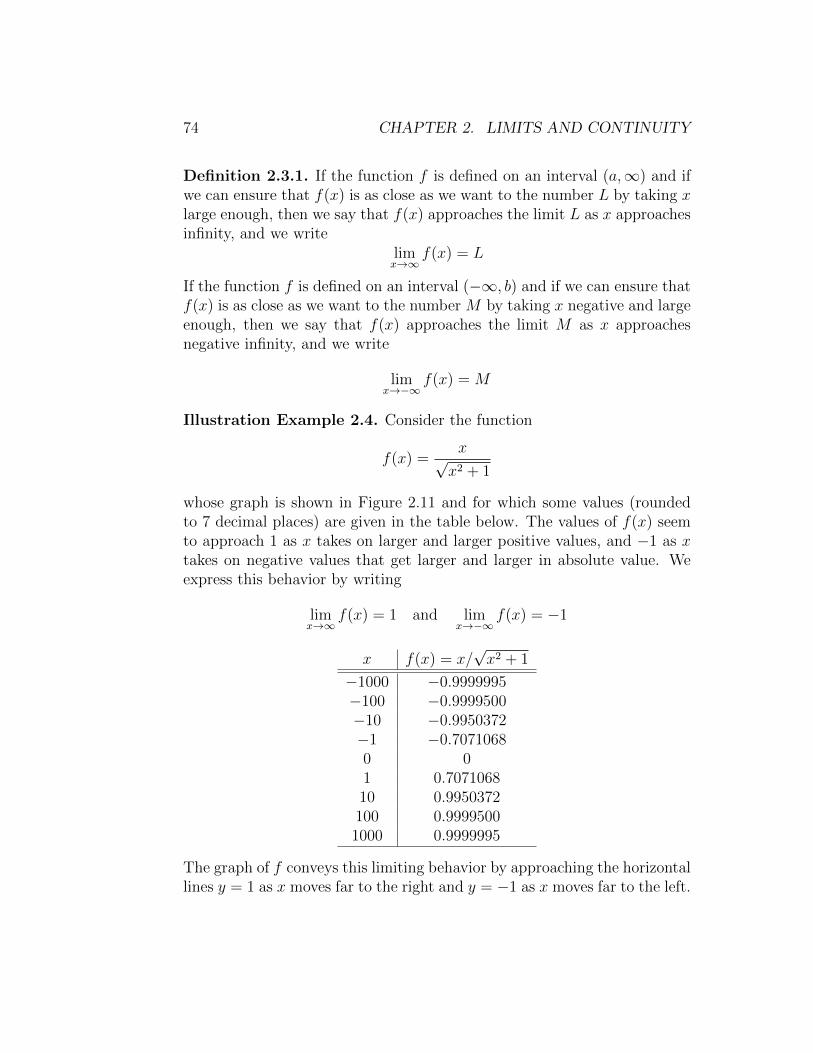
Illustration Example 2.4. Consider the function
f(x) =x√x2 + 1
whose graph is shown in Figure 2.11 and for which some values (roundedto 7 decimal places) are given in the table below. The values of f(x) seemto approach 1 as x takes on larger and larger positive values, and −1 as xtakes on negative values that get larger and larger in absolute value. Weexpress this behavior by writing
limx→∞
f(x) = 1 and limx→−∞
f(x) = −1
x f(x) = x/√x2 + 1
−1000 −0.9999995−100 −0.9999500−10 −0.9950372−1 −0.70710680 01 0.707106810 0.9950372100 0.99995001000 0.9999995
The graph of f conveys this limiting behavior by approaching the horizontallines y = 1 as x moves far to the right and y = −1 as x moves far to the left.
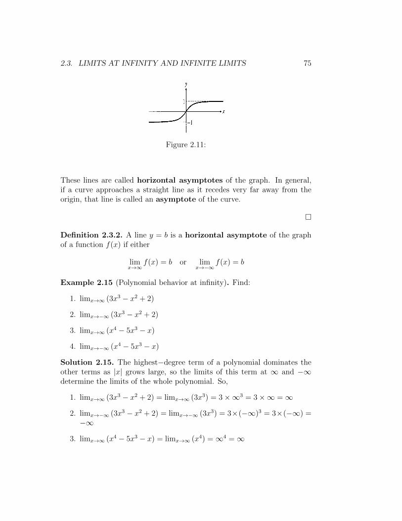
2.3. LIMITS AT INFINITY AND INFINITE LIMITS 75
Figure 2.11:
These lines are called horizontal asymptotes of the graph. In general,if a curve approaches a straight line as it recedes very far away from theorigin, that line is called an asymptote of the curve.
�
Definition 2.3.2. A line y = b is a horizontal asymptote of the graphof a function f(x) if either
limx→∞
f(x) = b or limx→−∞
f(x) = b
Example 2.15 (Polynomial behavior at infinity). Find:
1. limx→∞ (3x3 − x2 + 2)
2. limx→−∞ (3x3 − x2 + 2)
3. limx→∞ (x4 − 5x3 − x)
4. limx→−∞ (x4 − 5x3 − x)
Solution 2.15. The highest−degree term of a polynomial dominates theother terms as |x| grows large, so the limits of this term at ∞ and −∞determine the limits of the whole polynomial. So,
1. limx→∞ (3x3 − x2 + 2) = limx→∞ (3x3) = 3×∞3 = 3×∞ =∞
2. limx→−∞ (3x3 − x2 + 2) = limx→−∞ (3x3) = 3×(−∞)3 = 3×(−∞) =−∞
3. limx→∞ (x4 − 5x3 − x) = limx→∞ (x4) =∞4 =∞
76 CHAPTER 2. LIMITS AND CONTINUITY
4. limx→−∞ (x4 − 5x3 − x) = limx→−∞ (x4) = (−∞)4 =∞
�
The only polynomials that have limits at ±∞ are constant ones, P (x) =c. The situation is more interesting for rational functions. Recall that arational function is a quotient of two polynomials. The following examplesshow how to render such a function in a form where its limits at infinityand negative infinity (if they exist) are apparent. The way to do this is: todivide the numerator and denominator by the highest power of xappearing in the denominator, then use the following theorem.
Theorem 2.3.1. If r > 0 is a rational number such that xr is defined forall x, then
limx→±∞
1
xr= 0
Remark 2.3.1. The limits of a rational function at infinity and negative in-finity either both fail to exist or both exist and are equal.
Example 2.16. Evaluate
limx→±∞
2x2 − x+ 3
3x2 + 5
Solution 2.16. Divide the numerator and the denominator by x2 , thehighest power of x appearing in the denominator:
limx→±∞
2x2 − x+ 3
3x2 + 5= lim
x→±∞
2− (1/x) + (3/x2)
3 + (5/x2)
= limx→±∞
2− 0 + 0
3 + 0
=2
3
Therefore, y = 23
is horizontal asymptote of 2x2−x+33x2+5
.
�
2.3. LIMITS AT INFINITY AND INFINITE LIMITS 77
Example 2.17. Evaluate
limx→±∞
5x+ 2
2x3 − 1
Solution 2.17. Divide the numerator and the denominator by the largestpower of x in the denominator, namely, x3.
limx→±∞
5x+ 2
2x3 − 1= lim
x→±∞
(5/x2) + (2/x3)
2− (1/x3)
= limx→±∞
0 + 0
2− 0= 0
Therefore, y = 0 (the x−axis) is horizontal asymptote of 5x+22x3−1 .
�
Example 2.18. Evaluate
limx→∞
x3 + 1
x2 + 1
Solution 2.18. Divide the numerator and the denominator by x2, thelargest power of x in the denominator:
limx→∞
x3 + 1
x2 + 1= lim
x→∞
x+ (1/x2)
1 + (1/x2)
= limx→∞
∞+ 0
1 + 0= ∞
Also,
limx→−∞
x3 + 1
x2 + 1= −∞
Therefore the limits are not exist, and the function x3+1x2+1
has no horizontalasymptotes.
�
78 CHAPTER 2. LIMITS AND CONTINUITY
Summary of limits at ±∞ for rational functions Let
Pm(x) = amxm + · · ·+ a0
and Qn(x) = bnxn + · · ·+ b0
be polynomials of degree m and n, respectively, so that am 6= 0 andbn 6= 0. Then
limx→±∞
Pm(x)
Qn(x)
1. equals 0 if m < n,
2. equals ambn
if m = n,
3. does not exist if m > n.
The technique used in the previous examples can also be applied tomore general kinds of functions. The function in the following example isnot rational, and the limit seems to produce a meaningless∞−∞ until weresolve matters by rationalizing the numerator.
Example 2.19. Evaluate
limx→∞
(√x2 + x− x
)Solution 2.19. We are trying to find the limit of the difference of twofunctions, each of which becomes arbitrarily large as x increases to infin-ity. We rationalize the expression by multiply ing the numerator and thedenominator (which is 1) by the conjugate expression,
√x2 + x+ x:
limx→∞
(√x2 + x− x
)= lim
x→∞
(√x2 + x− x
) (√x2 + x+ x
)√x2 + x+ x
= limx→∞
x2 + x− x2√x2(1 + 1
x
)+ x
= limx→∞
x
x√
1 + 1x
+ x= lim
x→∞
1√1 + 1
x+ 1
=1
2
Here√x2 = |x| = x because x > 0 as x→∞.

2.3. LIMITS AT INFINITY AND INFINITE LIMITS 79
Exercise 2.10. Evaluate
limx→−∞
(√x2 + x− x
)Example 2.20. Using the Squeezing Theorem, find the horizontal asymp-tote of the curve
f(x) = 2 +sinx
x
Solution 2.20. We are interested in the behavior as x→ ±∞. Since
0 ≤∣∣∣∣sinxx
∣∣∣∣ ≤ ∣∣∣∣1x∣∣∣∣
and
limx→±∞
∣∣∣∣1x∣∣∣∣ = 0,
we have
limx→±∞
∣∣∣∣sinxx∣∣∣∣ = 0
by the Squeezing Theorem. Hence,
limx→±∞
(2 +
sinx
x
)= 2 + 0 = 2,
and the line y = 2 is a horizontal asymptote of the curve on both left andright.
�
Example 2.21. Find the horizontal asymptotes (if any) of the followingfunctions.
1. f(x) = tan−1 x
2. g(x) = ex
Solution 2.21. 1. In fact,
limx→∞
tan−1 x =π
2and lim
x→−∞tan−1 x = −π
2
so both of the lines y = −π2
and y = π2
are horizontal asymptotes.

80 CHAPTER 2. LIMITS AND CONTINUITY
2. The graph of the natural exponential function ex has the line y = 0(the x−axis) as a horizontal asymptote. (The same is true of anyexponential function with base a > 1.) In fact
limx→−∞
ex = 0 while limx→∞
ex =∞
so the line y = 0 is horizontal asymptote of g(x) = ex.
�
Example 2.22. Use the definitions of the hyperbolic functions to find eachof the following limits.
1. limx→∞
tanhx
2. limx→−∞
sinhx
Solution 2.22. 1. limx→∞ tanhx = limx→∞ex−e−x
ex−e−x = limx→∞ex
ex= 1
2. limx→−∞ sinhx = limx→∞ex−e−x
2= limx→∞
−e−x
2= −∞
�
Exercise 2.11. Use the definitions of the hyperbolic functions to find eachof the following limits.
1. limx→−∞
tanhx
2. limx→∞
sinhx
3. limx→∞
sech x
Oblique Asymptotes If the degree of the numerator of a rational functionis one greater than the degree of the denominator, the graph hasan oblique (slanted) asymptote. We find an equation for theasymptote by dividing numerator by denominator to express f as alinear function plus a remainder that goes to zero as x→ ±∞ Heresan example.
Example 2.23. Find the oblique asymptote for the graph of
f(x) =2x2 − 3
7x+ 4
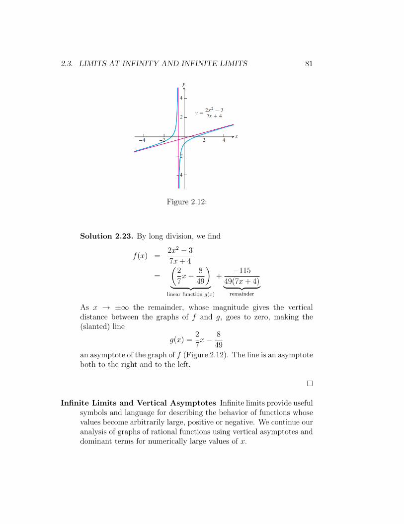
2.3. LIMITS AT INFINITY AND INFINITE LIMITS 81
Figure 2.12:
Solution 2.23. By long division, we find
f(x) =2x2 − 3
7x+ 4
=
(2
7x− 8
49
)︸ ︷︷ ︸
linear function g(x)
+−115
49(7x+ 4)︸ ︷︷ ︸remainder
As x → ±∞ the remainder, whose magnitude gives the verticaldistance between the graphs of f and g, goes to zero, making the(slanted) line
g(x) =2
7x− 8
49an asymptote of the graph of f (Figure 2.12). The line is an asymptoteboth to the right and to the left.
�
Infinite Limits and Vertical Asymptotes Infinite limits provide usefulsymbols and language for describing the behavior of functions whosevalues become arbitrarily large, positive or negative. We continue ouranalysis of graphs of rational functions using vertical asymptotes anddominant terms for numerically large values of x.

82 CHAPTER 2. LIMITS AND CONTINUITY
Figure 2.13:
Illustration Example 2.5. Let us look again at the function f(x) =1x. As x→ 0+ the values of f grow without bound, eventually reach-
ing and surpassing every positive real number. That is, given anypositive real number B, however large, the values of f become largerstill (Figure 2.13). Thus, f has no limit as x → 0+. It is never-theless convenient to describe the behavior of f by saying that f(x)approaches ∞ as x→ 0+. We write
limx→0+
f(x) = limx→0+
1
x=∞
In writing this, we are not saying that the limit exists. Nor are wesaying that there is a real number ∞, for there is no such number.Rather, we are saying that limx→0+
1x
does not exist because 1x
becomesarbitrarily large and positive as x → 0+. As x → 0−, the values off(x) = 1
xbecome arbitrarily large and negative. Given any negative
real number −B, the values of f eventually lie below −B. (See Figure2.13.) We write
limx→0−
f(x) = limx→0−
1
x= −∞
Again, we are not saying that the limit exists and equals the number−∞. There is no real number −∞. We are describing the behavior
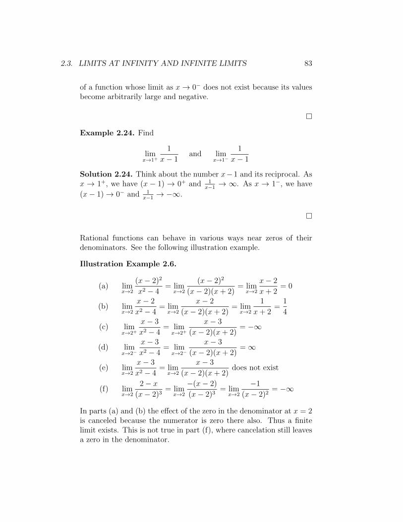
2.3. LIMITS AT INFINITY AND INFINITE LIMITS 83
of a function whose limit as x→ 0− does not exist because its valuesbecome arbitrarily large and negative.
�
Example 2.24. Find
limx→1+
1
x− 1and lim
x→1−
1
x− 1
Solution 2.24. Think about the number x−1 and its reciprocal. Asx → 1+, we have (x − 1) → 0+ and 1
x−1 → ∞. As x → 1−, we have
(x− 1)→ 0− and 1x−1 → −∞.
�
Rational functions can behave in various ways near zeros of theirdenominators. See the following illustration example.
Illustration Example 2.6.
(a) limx→2
(x− 2)2
x2 − 4= lim
x→2
(x− 2)2
(x− 2)(x+ 2)= lim
x→2
x− 2
x+ 2= 0
(b) limx→2
x− 2
x2 − 4= lim
x→2
x− 2
(x− 2)(x+ 2)= lim
x→2
1
x+ 2=
1
4
(c) limx→2+
x− 3
x2 − 4= lim
x→2+
x− 3
(x− 2)(x+ 2)= −∞
(d) limx→2−
x− 3
x2 − 4= lim
x→2−
x− 3
(x− 2)(x+ 2)=∞
(e) limx→2
x− 3
x2 − 4= lim
x→2
x− 3
(x− 2)(x+ 2)does not exist
(f) limx→2
2− x(x− 2)3
= limx→2
−(x− 2)
(x− 2)3= lim
x→2
−1
(x− 2)2= −∞
In parts (a) and (b) the effect of the zero in the denominator at x = 2is canceled because the numerator is zero there also. Thus a finitelimit exists. This is not true in part (f), where cancelation still leavesa zero in the denominator.

84 CHAPTER 2. LIMITS AND CONTINUITY
�
Definition 2.3.3. A line x = a is a vertical asymptote of the graphof a function f(x) if either
limx→a+
f(x) = ±∞ or limx→a−
f(x) = ±∞
Example 2.25. Find the horizontal and vertical asymptotes of thecurve
f(x) =x+ 3
x+ 2
Solution 2.25. We are interested in the behavior as x → ±∞ andas x→ −2 where the denominator is zero. Since
limx→±∞
x+ 3
x+ 2= lim
x→±∞
1 + 3x
1 + 2x
= 1
and
limx→−2+
x+ 3
x+ 2=∞ and lim
x→−2+
x+ 3
x+ 2= −∞
then: the horizontal asymptote is y = 1 and the vertical asymptote isx = −2.
�
Example 2.26. Find the horizontal and vertical asymptotes of thecurve
g(x) =−8
x2 − 4
Solution 2.26. We are interested in the behavior as x → ±∞ andas x → ±2 where the denominator is zero. Notice that g is an evenfunction of x, so its graph is symmetric with respect to the y−axis.Since
limx→±∞
−8
x2 − 4= 0
the line y = 0 is a horizontal asymptote of the graph of g. Since
limx→2+
−8
x2 − 4= −∞ and lim
x→2−
−8
x2 − 4=∞
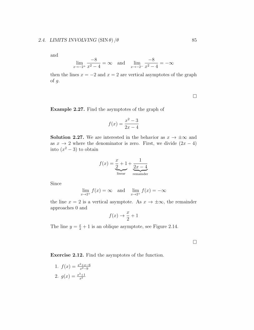
2.4. LIMITS INVOLVING (SIN θ) /θ 85
and
limx→−2+
−8
x2 − 4=∞ and lim
x→−2−
−8
x2 − 4= −∞
then the lines x = −2 and x = 2 are vertical asymptotes of the graphof g.
�
Example 2.27. Find the asymptotes of the graph of
f(x) =x2 − 3
2x− 4
Solution 2.27. We are interested in the behavior as x → ±∞ andas x → 2 where the denominator is zero. First, we divide (2x − 4)into (x2 − 3) to obtain
f(x) =x
2+ 1︸ ︷︷ ︸
linear
+1
2x− 4︸ ︷︷ ︸remainder
Since
limx→2+
f(x) =∞ and limx→2+
f(x) = −∞
the line x = 2 is a vertical asymptote. As x → ±∞, the remainderapproaches 0 and
f(x)→ x
2+ 1
The line y = x2
+ 1 is an oblique asymptote, see Figure 2.14.
�
Exercise 2.12. Find the asymptotes of the function.
1. f(x) = x2+x−6x2−9
2. g(x) = x3+1x2
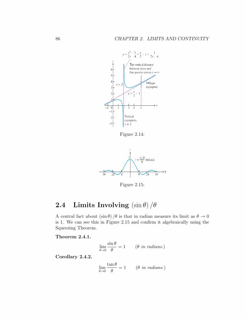
86 CHAPTER 2. LIMITS AND CONTINUITY
Figure 2.14:
Figure 2.15:
2.4 Limits Involving (sin θ) /θ
A central fact about (sin θ) /θ is that in radian measure its limit as θ → 0is 1. We can see this in Figure 2.15 and confirm it algebraically using theSqueezing Theorem.
Theorem 2.4.1.
limθ→0
sin θ
θ= 1 (θ in radians.)
Corollary 2.4.2.
limθ→0
tan θ
θ= 1 (θ in radians.)

2.4. LIMITS INVOLVING (SIN θ) /θ 87
Corollary 2.4.3.
(1) limθ→0
sin aθ
bθ= lim
θ→0
aθ
sin bθ= lim
θ→0
sin aθ
sin bθ=a
b
(2) limθ→0
tan aθ
bθ= lim
θ→0
aθ
tan bθ= lim
θ→0
tan aθ
tan bθ=a
b
(3) limθ→0
tan aθ
sin bθ= lim
θ→0
sin aθ
tan bθ=a
b
Example 2.28. Show that
limx→0
1− cosx
x= 0
Solution 2.28. Using the half−angle formula cos x = 1 − 2 sin2 (x/2), wecalculate
limx→0
1− cosx
x= lim
x→0
1−[1− 2 sin2 (x/2)
]x
= limx→0
[2 sin
(12x)
xsin
(1
2x
)]
= 2× limx→0
sin(12x)
x× lim
x→0sin
(1
2x
)= 2× 1/2
1× 0 = 0
Exercise 2.13. Show that
limθ→0
1− cos θ
θ sin θ=
1
2
by:
a) using the half−angle formula as in the previous example,
b) multiplying both the nominator and denominator by 1 + cos θ.
Example 2.29. Evaluate
limx→0
5 sin 3x+ tan 7x
3x+ x2
88 CHAPTER 2. LIMITS AND CONTINUITY
Solution 2.29.
limx→0
5 sin 3x+ tan 7x
3x+ x2= lim
x→0
5 sin 3xx
+ tan 7xx
3xx
+ x2
x
= limx→0
5 sin 3xx
+ tan 7xx
3 + x
=5× 3
1+ 7
1
3 + 0=
22
3
�
Exercise 2.14. Evaluate
limx→0
4x
tan 3x+ sin 2x
Example 2.30. Evaluate
limt→0
sin (t2)
t
Solution 2.30.
limt→0
sin (t2)
t= lim
t→0
[sin (t2)
t2× t]
= limt→0
sin (t2)
t2× lim
t→0t
= 1× 0 = 0
Example 2.31. Evaluate
limt→0
sin2 t
3t2
Solution 2.31.
limt→0
sin2 t
3t2=
1
3limt→0
[sin t
t
]2=
1
3
[limt→0
sin t
t
]2=
1
3× (1)2 =
1
3
�

2.5. CONTINUOUS FUNCTIONS 89
Example 2.32. Evaluate
limt→5
tan(t− 5)
t2 − 25
Solution 2.32.
limt→5
tan(t− 5)
t2 − 25= lim
t→5
tan(t− 5)
(t− 5)(t+ 5)
= limt→5
tan(t− 5)
t− 5× lim
t→5
1
t+ 5= 1× 1
5 + 5=
1
10
�
Exercise 2.15. Evaluate
limx→1
sin(πx)
x− 1and lim
x→0
tanx
|x|
2.5 Continuous Functions
We noticed in Section 2.2 that the limit of a function as x approaches a canoften be found simply by calculating the value of the function at a. Func-tions with this property are called continuous at a. We will see that themathematical definition of continuity corresponds closely with the meaningof the word continuity in everyday language. (A continuous process is onethat takes place gradually, without interruption or abrupt change.)
Definition 2.5.1. A function f is continuous at a number a if
limx→a
f(x) = f(a)
Notice that Definition 2.5.1 implicitly requires three things if f is con-tinuous at a:
1. f(a) is defined (that is, a is in the domain of f)
2. limx→a f(x) exists
3. limx→a f(x) = f(a).
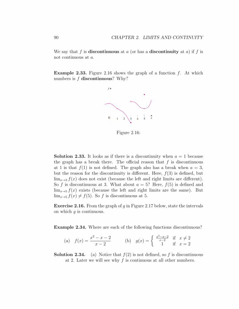
90 CHAPTER 2. LIMITS AND CONTINUITY
We say that f is discontinuous at a (or has a discontinuity at a) if f isnot continuous at a.
Example 2.33. Figure 2.16 shows the graph of a function f . At whichnumbers is f discontinuous? Why?
Figure 2.16:
Solution 2.33. It looks as if there is a discontinuity when a = 1 becausethe graph has a break there. The official reason that f is discontinuousat 1 is that f(1) is not defined. The graph also has a break when a = 3,but the reason for the discontinuity is different. Here, f(3) is defined, butlimx→3 f(x) does not exist (because the left and right limits are different).So f is discontinuous at 3. What about a = 5? Here, f(5) is defined andlimx→5 f(x) exists (because the left and right limits are the same). Butlimx→5 f(x) 6= f(5). So f is discontinuous at 5.
Exercise 2.16. From the graph of g in Figure 2.17 below, state the intervalson which g is continuous.
Example 2.34. Where are each of the following functions discontinuous?
(a) f(x) =x2 − x− 2
x− 2(b) g(x) =
{x2−x−2x−2 if x 6= 2
1 if x = 2
Solution 2.34. (a) Notice that f(2) is not defined, so f is discontinuousat 2. Later we will see why f is continuous at all other numbers.
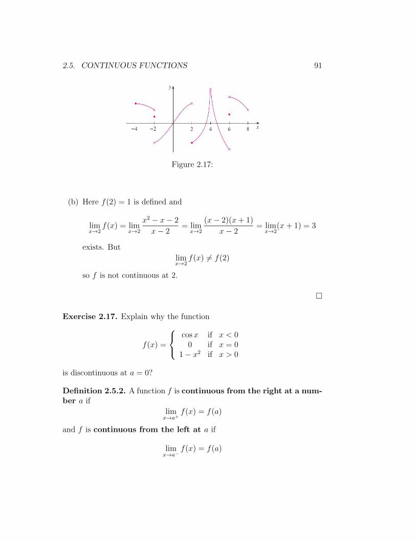
2.5. CONTINUOUS FUNCTIONS 91
Figure 2.17:
(b) Here f(2) = 1 is defined and
limx→2
f(x) = limx→2
x2 − x− 2
x− 2= lim
x→2
(x− 2)(x+ 1)
x− 2= lim
x→2(x+ 1) = 3
exists. But
limx→2
f(x) 6= f(2)
so f is not continuous at 2.
�
Exercise 2.17. Explain why the function
f(x) =
cosx if x < 0
0 if x = 01− x2 if x > 0
is discontinuous at a = 0?
Definition 2.5.2. A function f is continuous from the right at a num-ber a if
limx→a+
f(x) = f(a)
and f is continuous from the left at a if
limx→a−
f(x) = f(a)
92 CHAPTER 2. LIMITS AND CONTINUITY
Definition 2.5.3. A function f is continuous on an interval if it iscontinuous at every number in the interval. (If f is defined only on one sideof an endpoint of the interval, we understand continuous at the endpointto mean continuous from the right or continuous from the left.)
Example 2.35. Show that the function f(x) = 1−√
1− x2 is continuouson the interval [−1, 1].
Solution 2.35. If −1 < a < 1, then using the Limit Laws, we have
limx→a
f(x) = limx→a
(1−√
1− x2)
= 1− limx→a
√1− x2
= 1−√
1− a2
= f(a)
Thus, by Definition 2.5.1, f is continuous at a if −1 < a < 1. Similarcalculations show that
limx→−1+
f(x) = 1 = f(−1) and limx→1−
f(x) = 1 = f(1)
so f is continuous from the right at −1 and continuous from the left at 1.Therefore, according to Definition 2.5.3, f is continuous on [−1, 1].
�
Instead of always using Definitions 2.5.1, 2.5.2, and 2.5.3 to verify thecontinuity of a function as we did in the previous example, it is often con-venient to use the next two theorems, which shows how to build up com-plicated continuous functions from simple ones.
Theorem 2.5.1. If f and g are continuous at a and c is a constant, thenthe following functions are also continuous at a:
1. f + g 2. f − g 3. cf
4. f × g 5. fg
if g(a) 6= 0
Note that if f and g are continuous on an interval, then so are thefunctions f + g, f − g, fg, and f/g (if g is never 0).
2.5. CONTINUOUS FUNCTIONS 93
Theorem 2.5.2. All functions, except possibly piecewise functions, are con-tinuous on its domain.
Example 2.36. Find the points of discontinuity of the following.
1. f(x) = 13−|x|
2. f(x) = 2 ln√
1− x
3. f(x) = 5 + 21/x
4. f(x) =
{2x− 3 if x ≤ 41 + 16
xif x > 4
Solution 2.36. 1. Since the domain of f(x) = 13−|x| is R−{−3, 3} then
f is continuous on R− {−3, 3} and discontinuous on {−3, 3}.
2. Since the domain of f(x) = 2 ln√
1− x is (−∞, 1) then f is continu-ous on (−∞, 1) and discontinuous on R− (−∞, 1) = [1,∞).
3. Since the domain of f(x) = 5 + 21/x is R − {0} then f is continuouson R− {0} and discontinuous only when x = 0.
4. Note that f is piecewise function. Since f(x) = 2x−3 when x < 4 thenit is continuous because 2x−3 is a polynomial continuous everywhereand has no discontinuity point. When x > 4, f(x) = 1 + 16
xalso
continuous, although it is discontinuous at x = 0 but 0 ≯ 4. So, theonly possible discontinuity points of f(x) is x = 4. However, f(x) iscontinuous at x = 4 because:
a) f(4) = 2× 4− 3 = 5 is defined,
b) Since
limx→4+
f(x) = limx→4+
(1 +
16
x
)= 5
limx→4−
f(x) = limx→4−
(2x− 3) = 5
then limx→4 f(x) exists and equals 5.
c) f(4) = limx→4 f(x) = 5.

94 CHAPTER 2. LIMITS AND CONTINUITY
Hence, f(x) is continuous on R and has no discontinuity point.
�
Exercise 2.18. Where is the function
g(x) =lnx+ tan−1 x
x2 − 1
continuous?
Example 2.37. For what value of the constant c is the function continuouson (−∞,∞)?
f(x) =
{cx2 + 2x if x < 2x3 − cx if x ≥ 2
Solution 2.37. Because f is continuous on R = (−∞,∞) then it is con-tinuous at x = 2 the piecewise point of f . Therefore, limx→2 f(x) exists,and
limx→2+
f(x) = limx→2−
f(x)
limx→2+
(x3 − cx
)= lim
x→2−
(cx2 + 2x
)8− 2c = 4c+ 4
6c = 4
c =4
6=
2
3
�
Exercise 2.19. Find the values of a and b that make the function contin-uous everywhere.
(a) f(x) =
{(sin ax)/5x if x 6= 0
2 if x = 0
(b) g(x) =
(x2 − 4)/(x− 2) if x < 2ax2 − bx+ 3 if 2 ≤ x < 32x− a+ b if x ≥ 3
2.5. CONTINUOUS FUNCTIONS 95
Another way of combining continuous functions f and g to get a newcontinuous function is to form the composite function f ◦ g. This fact is aconsequence of the following theorem.
Theorem 2.5.3. If g is continuous at a and f is continuous at g(a), thenthe composite function (f ◦ g) (x) = f(g(x)) is continuous at a.
Theorem 2.5.4. If f is continuous at b and limx→a g(x) = b then
limx→a
f (g(x)) = f(b)
In other words,
limx→a
f (g(x)) = f(
limx→a
g(x))
Example 2.38. Evaluate
limx→1
sin−1(
1−√x
1− x
)Solution 2.38. Because sin−1 is a continuous function, we can apply The-orem 2.5.4:
limx→1
sin−1(
1−√x
1− x
)= sin−1
(limx→1
1−√x
1− x
)= sin−1
(limx→1
1− x(1−
√x) (1 +
√x)
)= sin−1
(limx→1
1
1 +√x
)= sin−1
(1
2
)=π
6
Exercise 2.20. Use continuity to evaluate limx→π sin (x+ sinx).


Chapter 3
The Derivative
The derivative is a limit measures the rate at which a function changesand is one of the most important ideas in calculus. Derivatives are usedwidely in science, economics, medicine, and computer science to calculatevelocity and acceleration, to explain the behavior of machinery, to estimatethe drop in water levels as water is pumped out of a tank, and to predictthe consequences of making errors in measurements. Finding derivativesby evaluating limits can be lengthy and difficult. We develop techniques tomake calculating derivatives easier.
3.1 The Derivative as a Function
The problem of finding the tangent line to a curve involves finding a typeof limit. This special type of limit is called a derivative.
Definition 3.1.1. The derivative of the function f(x) with respect to thevariable x is the function f ′ whose value at x is
f ′(x) = limh→0
f(x+ h)− f(x)
h
= limw→x
f(w)− f(x)
w − xprovided the limit exists.
The domain of f ′ is the set of points in the domain of f for which thelimit exists, and the domain may be the same or smaller than the domain
97

98 CHAPTER 3. THE DERIVATIVE
of f . If f ′ exists at a particular x, we say that f is differentiable (has aderivative) at x. If f ′ exists at every point in the domain of f , we call fdifferentiable.
Notations There are many ways to denote the derivative of a functiony = f(x) where the independent variable is x and the dependentvariable is y. Some common alternative notations for the derivativeare
f ′(x) = y′ =dy
dx=df
dx=
d
dxf(x) = D(f)(x) = Dxf(x)
The symbols d/dx and D indicate the operation of differentiationand are called differentiation operators. We read dy/dx as thederivative of y with respect to x, and df/dx and (d/dx)f(x) as thederivative of f with respect to x. The prime notations y′ and f ′ comefrom notations that Newton used for derivatives. The d/dx notationsare similar to those used by Leibniz. The dy/dx symbol should notbe regarded as a ratio.
Be careful not to confuse the notation D(f) as meaning the domainof the function f instead of the derivative function f ′. The distinctionshould be clear from the context.
To indicate the value of a derivative at a specified number x = a, weuse the notation
f ′(a) =dy
dx
∣∣∣∣x=a
=df
dx
∣∣∣∣x=a
=d
dxf(x)
∣∣∣∣x=a
Calculating Derivatives from the Definition The process of calculat-ing a derivative is called differentiation. To emphasize the idea thatdifferentiation is an operation performed on a function y = f(x) weuse the notation
d
dxf(x)
as another way to denote the derivative f ′(x).
Example 3.1. Differentiate f(x) = x2.

3.1. THE DERIVATIVE AS A FUNCTION 99
Solution 3.1.
f ′(x) = limh→0
f(x+ h)− f(x)
h
= limh→0
(x+ h)2 − x2
h
= limh→0
x2 + 2xh− h2 − x2
h
= limh→0
2xh− h2
h
= limh→0
h(2x− h)
h= lim
h→0(2x− h) = 2x
�
Example 3.2. Find the derivative of g(x) =√x at x = 4.
Solution 3.2.
g′(x) = limw→x
f(w)− f(x)
w − x
= limw→x
√w −√x
w − x
= limw→x
√w −√x
(√w −√x) (√w +√x)
= limw→x
1√w +√x
=1
2√x
g′(4) =1
2×√
4=
1
4
�
Exercise 3.1. Find the derivative of f(t) = 1/t at t = 5.
Differentiable on an Interval; One-Sided Derivatives A function y =f(x) is differentiable on an open interval (finite or infinite) if it hasa derivative at each point of the interval. It is differentiable on a

100 CHAPTER 3. THE DERIVATIVE
closed interval [a, b] if it is differentiable on the interior (a, b) and ifthe limits
f ′+(a) = limh→0+
f(a+ h)− f(a)
hRight−hand derivative at a
f ′−(b) = limh→0−
f(b+ h)− f(b)
hLeft−hand derivative at b
exist at the endpoints.
Right−hand and left−hand derivatives may be defined at any point ofa function’s domain. The usual relation between one-sided and two-sided limits holds for these derivatives. A function has a deriva-tive at a point if and only if it has left-hand and right-handderivatives there, and these one-sided derivatives are equal.
f ′ (x0) exists ⇔ f ′+ (x0) = f ′− (x0) and both are exist.
Example 3.3. Show that the function g(x) = |x| is not differentiableat x = 0.
Solution 3.3. There can be no derivative at the origin because theone−sided derivatives differ there:
g′+(0) = limh→0+
g(0 + h)− g(0)
h
= limh→0+
|0 + h| − |0|h
= limh→0+
|h|h
= limh→0+
h
h= lim
h→0+1 = 1
g′−(0) = limh→0−
g(0 + h)− g(0)
h
= limh→0−
|0 + h| − |0|h
= limh→0−
|h|h
= limh→0−
−hh
= limh→0−
−1 = −1
�
Exercise 3.2. Show that the function f(x) =√x is not differentiable
at x = 0.

3.1. THE DERIVATIVE AS A FUNCTION 101
When Does a Function Not Have a Derivative at a Point?Differentiability is a smoothness condition on the graph of f . Afunction whose graph is otherwise smooth will fail to have a derivativeat a point for several reasons, such as at points where the graph has(see Figure 3.1)
1. a corner, where the one-sided derivatives differ.
2. a cusp, where the derivative approaches ∞ from one side and−∞ from the other.
3. a vertical tangent, where the derivative approaches∞ from bothsides or −∞ from both sides.
4. a discontinuity.
Figure 3.1:
Differentiable Functions Are Continuous A function is continuous atevery point where it has a derivative.
Theorem 3.1.1. If f has a derivative at x = c, then f is continuousat x = c.
Corollary 3.1.2. If f is discontinuous at x = c, then f is not differ-entiable at x = c.
Note that a function need not have a derivative at a point where it iscontinuous. Also, a function that is not differentiable at a point neednot be discontinuous at that point. For example, |x| is continuous atx = 0 but it is not differentiable at x = 0.
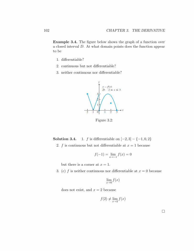
102 CHAPTER 3. THE DERIVATIVE
Example 3.4. The figure below shows the graph of a function overa closed interval D. At what domain points does the function appearto be
1. differentiable?
2. continuous but not differentiable?
3. neither continuous nor differentiable?
Figure 3.2:
Solution 3.4. 1. f is differentiable on [−2, 3]− {−1, 0, 2}2. f is continuous but not differentiable at x = 1 because
f(−1) = limx→−1
f(x) = 0
but there is a corner at x = 1.
3. (c) f is neither continuous nor differentiable at x = 0 because
limx→0
f(x)
does not exist, and x = 2 because
f(2) 6= limx→2
f(x)
�
3.2. DIFFERENTIATION RULES AND HIGHER DERIVATIVES 103
3.2 Differentiation Rules and Higher
Derivatives
This section introduces rules that allow us to differentiate a great varietyof functions. By these rules, we can differentiate functions without havingto apply the definition of the derivative each time.
Rule 1 If f has the constant value f(x) = c then
df
dx=
d
dx(c) = 0.
The first rule of differentiation is that the derivative of every constantfunction is zero. For example,
d
dx(8) = 0,
d
dx(π) = 0,
d
dx
(√e)
= 0.
Rule 2 If n is a real number, then
d
dxxn = nxn−1.
The second rule tells how to differentiate xn if n is a real number. Forexample,
(1)d
dx(x) = 1
(2)d
dx
(x2)
= 2x
(3)d
dx
(x3)
= 3x2
(4)d
dx
(x4)
= 4x3
(5)d
dx
(1
x2
)=
d
dx
(x−2)
= −2x−3 =−2
x3
(6)d
dx
(3√x4)
=d
dx
(x4/3
)=
4
3x1/3 =
4
33√x

104 CHAPTER 3. THE DERIVATIVE
Rule 3 If u is a differentiable function of x, and c is a constant, then
d
dx(cu) = c
du
dx.
The third rule says that when a differentiable function is multipliedby a constant, its derivative is multiplied by the same constant. Forexample,
d
dx
(3x2)
= 3d
dx
(x2)
= 3× (2x) = 6x.
Rule 4 If u and v are differentiable functions of x, then their sum (ordifference) u ± v is differentiable at every point where u and v areboth differentiable. At such points,
d
dx(u± v) =
du
dx± dv
dx
This rule says that the derivative of the sum (or difference) of twodifferentiable functions is the sum of their derivatives. For example,if f(x) = x3 + 4
3x2 − 5x+ 1 then
f ′(x) =d
dx
(x3 +
4
3x2 − 5x+ 1
)=
d
dx
(x3)
+d
dx
(4
3x2)− d
dx(5x) +
d
dx(1)
=d
dx
(x3)
+4
3
d
dx
(x2)− 5
d
dx(x) +
d
dx(1)
= 3x2 +4
3× 2x− 5× 1 + 0
= 3x2 +8
3x− 5
Rule 5 While the derivative of the sum of two functions is the sum oftheir derivatives, the derivative of the product of two functions is notthe product of their derivatives. The derivative of a product of twofunctions is the sum of two products, as we now explain. If u and vare differentiable at x, then so is their product uv, and
d
dx(uv) = u
dv
dx+ v
du
dx

3.2. DIFFERENTIATION RULES AND HIGHER DERIVATIVES 105
For example,
d
dx
[x(1− x2
)]= x
d
dx
(1− x2
)+(1− x2
) d
dx(x)
= x(−2x) +(1− x2
)(1)
= −2x2 + 1− x2
= 1− 3x2
Rule 6 Just as the derivative of the product of two differentiable functionsis not the product of their derivatives, the derivative of the quotient oftwo functions is not the quotient of their derivatives. What happensinstead is the Quotient Rule: If u and v are differentiable at x and ifv(x) 6= 0 then the quotient u/v is differentiable at x, and
d
dx
(uv
)=v dudx− u dv
dx
v2.
For example,
d
dt
(t2 − 1
t2 + 1
)=
(t2 + 1) ddt
(t2 − 1)− (t2 − 1) ddt
(t2 + 1)
(t2 + 1)2
=(t2 + 1) (2t)− (t2 − 1) (2t)
(t2 + 1)2
=2t3 + 2t− 2t3 + 2t
(t2 + 1)2
=4t
(t2 + 1)2
Rule 7 The derivative of the sine function is the cosine function:
d
dx(sinx) = cos x
The following is an example of derivative of function involving thesine function.
d
dx
(2x3 sinx
)= 2x3
d
dx(sinx) + sin x
d
dx(2x3) = 2x3 cosx+ 6x2 sinx
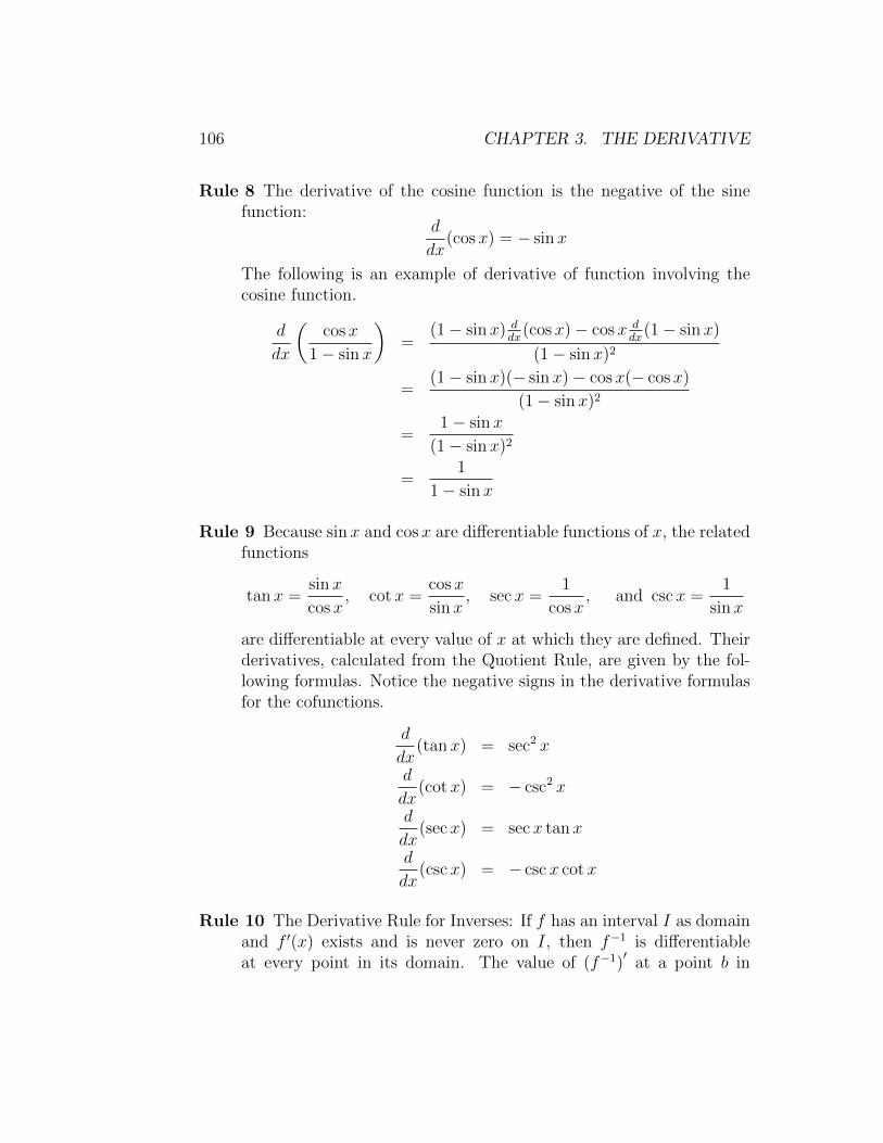
106 CHAPTER 3. THE DERIVATIVE
Rule 8 The derivative of the cosine function is the negative of the sinefunction:
d
dx(cosx) = − sinx
The following is an example of derivative of function involving thecosine function.
d
dx
(cosx
1− sinx
)=
(1− sinx) ddx
(cosx)− cosx ddx
(1− sinx)
(1− sinx)2
=(1− sinx)(− sinx)− cosx(− cosx)
(1− sinx)2
=1− sinx
(1− sinx)2
=1
1− sinx
Rule 9 Because sinx and cosx are differentiable functions of x, the relatedfunctions
tanx =sinx
cosx, cotx =
cosx
sinx, secx =
1
cosx, and cscx =
1
sinx
are differentiable at every value of x at which they are defined. Theirderivatives, calculated from the Quotient Rule, are given by the fol-lowing formulas. Notice the negative signs in the derivative formulasfor the cofunctions.
d
dx(tanx) = sec2 x
d
dx(cotx) = − csc2 x
d
dx(secx) = secx tanx
d
dx(cscx) = − cscx cotx
Rule 10 The Derivative Rule for Inverses: If f has an interval I as domainand f ′(x) exists and is never zero on I, then f−1 is differentiableat every point in its domain. The value of (f−1)
′at a point b in

3.2. DIFFERENTIATION RULES AND HIGHER DERIVATIVES 107
the domain of f−1 is the reciprocal of the value of f ′ at the pointa = f−1(b): (
f−1)′
(b) =1
f ′ (f−1(b))
Example 3.5. Let f(x) = x3 − 2. Find the value of df−1/dx atx = 6 = f(2) without finding a formula for f−1(x)
Solution 3.5.(f−1)′
(6) =1
f ′ (f−1(6))=
1
f ′(2)=
1
3× 22=
1
12
�
Exercise 3.3. Let f(x) = 2x+ 3. Find f−1(x), then evaluate df/dxat x = −1 and df−1/dx at x = f(−1) to show that(
f−1)′
(−1) =1
f ′ (f−1(−1))
Rule 11 For every positive value of x, we have
d
dx(lnx) =
1
x, and in general
d
dx(loga x) =
1
x ln a.
For example,
d
dt(t ln t) = t
d
dt(ln t) + ln t
d
dt(t) = t× 1
t+ ln t = 1 + ln t
d
dt(2 log10 t) = 2
d
dt(log10 t) = 2× 1
t ln 10=
2
t ln 10
Rule 12 The exponential function is differentiable because it is the inverseof a differentiable function whose derivative is never zero. So, by Rule10, we have
d
dx(ex) = ex, and in general
d
dx(ax) = ax ln a.
For example,
d
dt
(tan t
10t
)=
10t ddt
(tan t)− tan t ddt
(10t)
(10t)2
=10t sec2 t− 10t(ln 10) tan t
102t=
sec2 t− (ln 10) tan t
10t
108 CHAPTER 3. THE DERIVATIVE
Rule 13 The derivatives of the inverse trigonometric functions are sum-marized as follows.
(1)d
dx(sin−1 x) =
1√1− x2
where |x| < 1
(2)d
dx(cos−1 x) =
−1√1− x2
where |x| < 1
(3)d
dx(tan−1 x) =
1
1 + x2
(4)d
dx(cot−1 x) =
−1
1 + x2
(5)d
dx(sec−1 x) =
1
|x|√x2 − 1
where |x| > 1
(6)d
dx(csc−1 x) =
−1
|x|√x2 − 1
where |x| > 1
Rule 14 Derivatives of Hyperbolic Functions.
(1)d
dx(sinhx) = cosh x
(2)d
dx(coshx) = sinhx
(3)d
dx(tanhx) = sech2x
(4)d
dx(cothx) = −csch2x
(5)d
dx(sech x) = −sech x tanhx
(6)d
dx(csch x) = −csch x cothx
Rule 15 Derivatives of Inverse Hyperbolic Functions.
(1)d
dx(sinh−1 x) =
1√1 + x2
(2)d
dx(cosh−1 x) =
1√x2 − 1
3.2. DIFFERENTIATION RULES AND HIGHER DERIVATIVES 109
(3)d
dx(tanh−1 x) =
1
1− x2
(4)d
dx(coth−1 x) =
1
1− x2
(5)d
dx(sech−1x) =
−1
x√
1− x2
(6)d
dx(csch−1x) =
−1
|x|√
1 + x2
Exercise 3.4. Find the derivative f ′ with respect to x of the followingfunctions.
1. f(x) = (1 + x)√x
2. f(x) = 2x − x2
3. f(x) = ex tan−1 x
4. f(x) = 2x2/(7x+ 5)
5. f(x) = x sinhx− coshx
Example 3.6. If f(x) =√xg(x) where g(4) = 2 and g′(4) = 3, find f ′(4).
Solution 3.6.
f ′(x) =d
dx
[√xg(x)
]=√xg′(x) + g(x)× 1
2√x
f ′(4) =√
4g′(4) + g(4)× 1
2√
4
= 2× 3 + 2× 1
4=
13
2
�
Example 3.7. For what values of a and b such that
f(x) =
{x2 + a if x ≤ 1bx if x > 1
is differentiable at x = 1.

110 CHAPTER 3. THE DERIVATIVE
Solution 3.7. Since f is differentiable at x = 1, then: f is continuous atx = 1, and f ′(1) exists. Therefore,
f ′(1) exists ⇒ f ′+(1) = f ′−(1)
⇒ d
dx(bx)
∣∣∣∣x=1
=d
dx
(x2 + a
)∣∣∣∣x=1
⇒ b = 2
f continuous at x = 1 ⇒ limx→1
f(x) exists
⇒ limx→1+
f(x) = limx→1−
f(x)
⇒ limx→1+
(bx) = limx→1−
(x2 + a
)⇒ b = 1 + a⇒ 2 = 1 + a⇒ a = 1
�
Exercise 3.5. For what values of m and b such that
g(x) =
{x2 if x ≤ 2mx+ b if x > 2
is differentiable at x = 2.
Remark 3.2.1.
limh→0
f(x+ ah)− f(x)
bh=a
bf ′(x)
Example 3.8. If f(x) = x+ lnx, evaluate
limh→0
f(2− 2h)− f(2)
3h
Solution 3.8. Note that f ′(x) = 1 + 1/x. Therefore,
limh→0
f(2− 2h)− f(2)
3h=−2
3f ′(2)
=−2
3×(
1 +1
2
)=−2
3× 3
2= −1
3.2. DIFFERENTIATION RULES AND HIGHER DERIVATIVES 111
Exercise 3.6. Each limit represents the derivative of some function f atsome number c. State such an f and c in each case and then evaluate thelimit.
(1) limx→1
x9 − 1
x− 1
(2) limh→0
4√
16 + h− 2
h
Higher Derivatives If f(x) is a differentiable function, then its deriva-tive f ′(x) is also a function. If f ′ is also differentiable, then we candifferentiate to get a new function of x denoted by f ′′. So f ′′ = (f ′)′.The function f ′′ is called the second derivative of f because it isthe derivative of the first derivative. Notationally,
f ′′(x) =d2
dx2f(x) =
d
dx
[d
dxf(x)
]
If f ′′ is differentiable, its derivative
f ′′′(x) =d3
dx3f(x) =
d
dx
[d2
dx2f(x)
]
is the third derivative of f with respect to x. The names continueas you imagine, with
f (n)(x) =dn
dxnf(x) =
d
dx
[d(n−1)
dx(n−1)f(x)
]
denoting the nth derivative of f with respect to x for any pos-itive integer n.
Example 3.9. If f(x) = x3 − x, find f ′′′(x) and f (4)(x)

112 CHAPTER 3. THE DERIVATIVE
Solution 3.9.
f(x) = x3 − x
f ′(x) =d
dx
(x3 − x
)= 3x2 − 1
f ′′(x) =d
dx
(3x2 − 1
)= 6x
f ′′′(x) =d
dx(6x) = 6 = 3!
f (4)(x) =d
dx(6) = 0
�
Example 3.10. Find the 27th derivative of cosx.
Solution 3.10. The first few derivatives of f(x) = cos x are as follows:
f ′(x) = − sinx
f ′′(x) = − cosx
f ′′′(x) = sinx
f (4)(x) = cosx
f (5)(x) = − sinx
We see that the successive derivatives occur in a cycle of length 4 and,in particular, f (n)(x) = cos x whenever n is a multiple of 4. Therefore
f (24)(x) = cos x
and, differentiating three more times, we have
f (27)(x) = sin x
�
Exercise 3.7. Let f(x) = (x+ 1)/x. Evaluate: f ′′(x) and f ′′′(2).
Exercise 3.8. Evaluated87
dx87sinx

3.3. THE CHAIN RULE 113
Example 3.11. Find a formula of the general nth derivative of g(x) =xex.
Solution 3.11. To find the nth derivative of a function, good ideato start doing first few derivatives, and try to guess a formula fromthese derivatives. For the function g(x) = xex we have
g′(x) = xd
dx(ex) + ex
d
dx(x) = xex + ex = (x+ 1)ex
g′′(x) = (x+ 1)d
dx(ex) + ex
d
dx(x+ 1) = (x+ 1)ex + ex = (x+ 2)ex
g′′′(x) = (x+ 2)d
dx(ex) + ex
d
dx(x+ 2) = (x+ 2)ex + ex = (x+ 3)ex
g(4)(x) = (x+ 3)d
dx(ex) + ex
d
dx(x+ 3) = (x+ 3)ex + ex = (x+ 4)ex
...
g(n)(x) = (x+ n)ex
�
Exercise 3.9. Find a formula of the general nth derivative of:
1. f(x) = xn
2. f(x) = 1/x
3.3 The Chain Rule
Suppose you are asked to differentiate the function F (x) =√
1 + x2. Thedifferentiation formulas you learned in the previous sections of this chapterdo not enable you to calculate F ′(x). Observe that F is a composite func-tion. In fact, if we let y = f(u) =
√u and let u = g(x) = 1 + x2, then
we can write y = F (x) = f(g(x)), that is, F = f ◦ g. We know how todifferentiate both f and g, so it would be useful to have a rule that tells ushow to find the derivative of F = f ◦ g in terms of the derivatives of f andg.
It turns out that the derivative of the composite function f ◦ g is theproduct of the derivatives of f and g. This fact is one of the most importantof the differentiation rules and is called the Chain Rule.

114 CHAPTER 3. THE DERIVATIVE
The Chain Rule If g is differentiable at x and f is differentiable at g(x),then the composite function F = f ◦ g defined by F (x) = f(g(x)) isdifferentiable at x and F ′ is given by the product
F ′(x) = f ′(g(x)) · g′(x)
In Leibniz notation, if y = f(u) and u = g(x) are both differentiablefunctions, then
dy
dx=dy
du
du
dx
Example 3.12. Given that g(2) = 1/2, g′(2) = −1/4, and f ′(1/2) = 1,find (f ◦ g)′(2).
Solution 3.12.
(f ◦ g)′(2) = f ′(g(2)) · g′(2) = f ′(
1
2
)× −1
4= 1× −1
4=−1
4
�
Example 3.13. Let y = 5− et and t = 2x2 − 3. Find dy/dx at x = 1.
Solution 3.13. Here, y is a function of t and t is a function of x, so y is afunction of x. Note that when x = 1 we have t = 2× (1)2− 3 = −1. Hence,
dy
dx=dy
dt· dtdx
=(−et)× (4x)
anddy
dx
∣∣∣∣x=1t=−1
=(−e−1
)× (4) =
−4
e
�
When applying the Chain Rule, it is helpful to think of the compositefunction f ◦ g as having two parts, an inner part and an outer part. TheChain Rule tells you that the derivative of y = f(u) is the derivative of theouter function (at the inner function u) times the derivative of the innerfunction. That is,
y′ = f ′(u) · u′
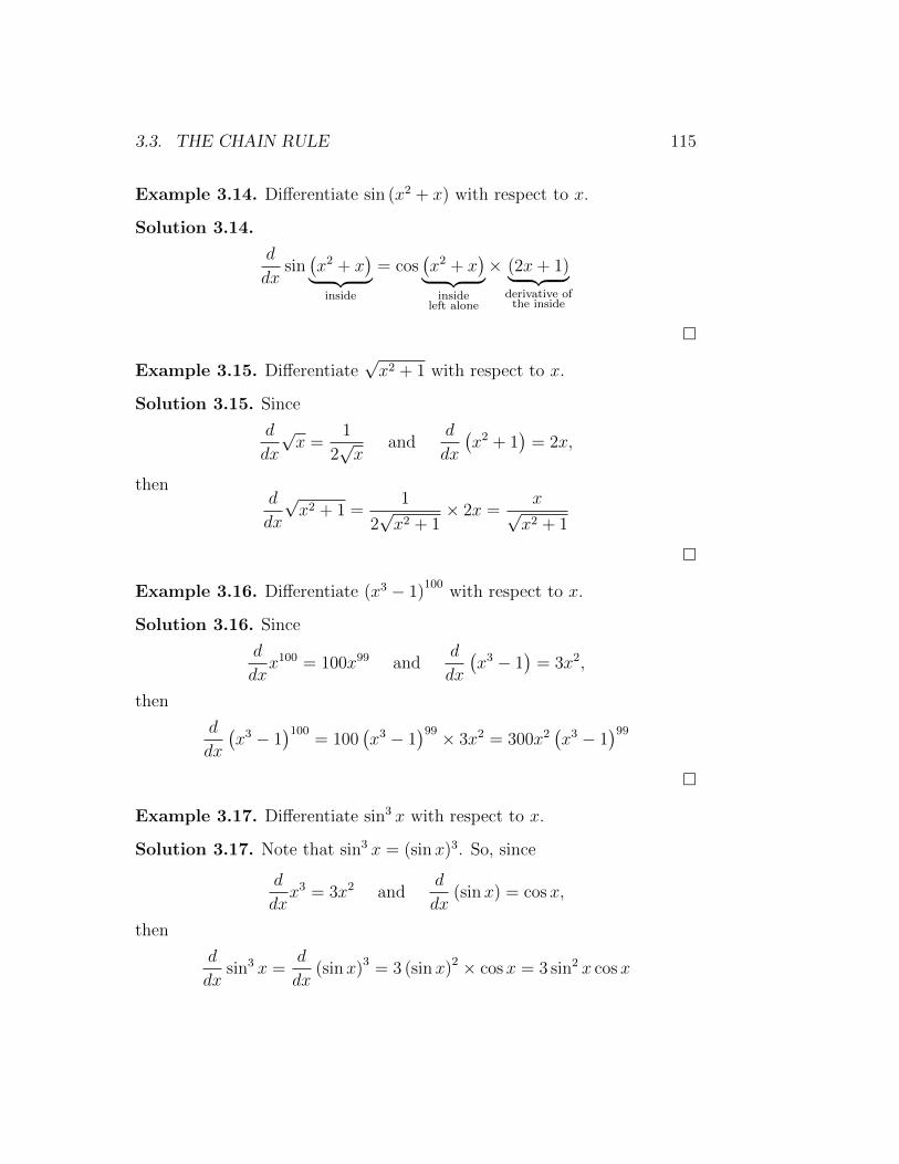
3.3. THE CHAIN RULE 115
Example 3.14. Differentiate sin (x2 + x) with respect to x.
Solution 3.14.
d
dxsin(x2 + x
)︸ ︷︷ ︸inside
= cos(x2 + x
)︸ ︷︷ ︸inside
left alone
× (2x+ 1)︸ ︷︷ ︸derivative ofthe inside
�
Example 3.15. Differentiate√x2 + 1 with respect to x.
Solution 3.15. Since
d
dx
√x =
1
2√x
andd
dx
(x2 + 1
)= 2x,
thend
dx
√x2 + 1 =
1
2√x2 + 1
× 2x =x√x2 + 1
�
Example 3.16. Differentiate (x3 − 1)100
with respect to x.
Solution 3.16. Since
d
dxx100 = 100x99 and
d
dx
(x3 − 1
)= 3x2,
then
d
dx
(x3 − 1
)100= 100
(x3 − 1
)99 × 3x2 = 300x2(x3 − 1
)99�
Example 3.17. Differentiate sin3 x with respect to x.
Solution 3.17. Note that sin3 x = (sinx)3. So, since
d
dxx3 = 3x2 and
d
dx(sinx) = cos x,
then
d
dxsin3 x =
d
dx(sinx)3 = 3 (sin x)2 × cosx = 3 sin2 x cosx
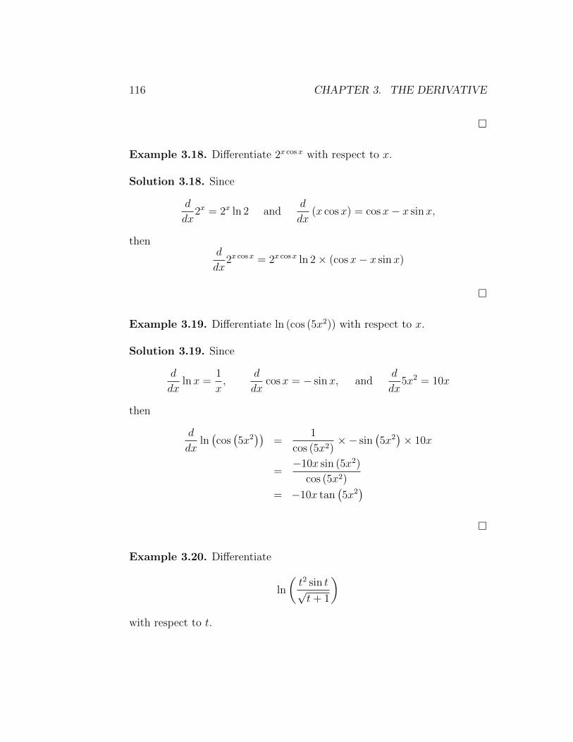
116 CHAPTER 3. THE DERIVATIVE
�
Example 3.18. Differentiate 2x cosx with respect to x.
Solution 3.18. Since
d
dx2x = 2x ln 2 and
d
dx(x cosx) = cos x− x sinx,
thend
dx2x cosx = 2x cosx ln 2× (cosx− x sinx)
�
Example 3.19. Differentiate ln (cos (5x2)) with respect to x.
Solution 3.19. Since
d
dxlnx =
1
x,
d
dxcosx = − sinx, and
d
dx5x2 = 10x
then
d
dxln(cos(5x2))
=1
cos (5x2)×− sin
(5x2)× 10x
=−10x sin (5x2)
cos (5x2)
= −10x tan(5x2)
�
Example 3.20. Differentiate
ln
(t2 sin t√t+ 1
)with respect to t.
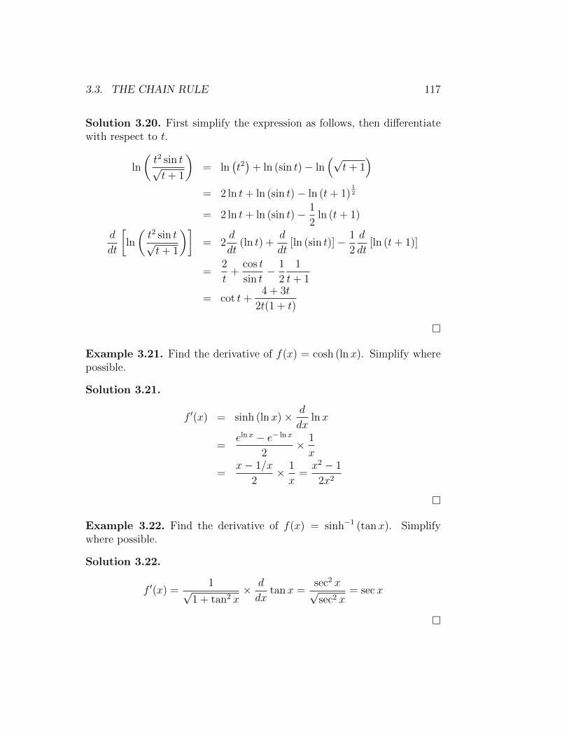
3.3. THE CHAIN RULE 117
Solution 3.20. First simplify the expression as follows, then differentiatewith respect to t.
ln
(t2 sin t√t+ 1
)= ln
(t2)
+ ln (sin t)− ln(√
t+ 1)
= 2 ln t+ ln (sin t)− ln (t+ 1)12
= 2 ln t+ ln (sin t)− 1
2ln (t+ 1)
d
dt
[ln
(t2 sin t√t+ 1
)]= 2
d
dt(ln t) +
d
dt[ln (sin t)]− 1
2
d
dt[ln (t+ 1)]
=2
t+
cos t
sin t− 1
2
1
t+ 1
= cot t+4 + 3t
2t(1 + t)
�
Example 3.21. Find the derivative of f(x) = cosh (ln x). Simplify wherepossible.
Solution 3.21.
f ′(x) = sinh (lnx)× d
dxlnx
=elnx − e− lnx
2× 1
x
=x− 1/x
2× 1
x=x2 − 1
2x2
�
Example 3.22. Find the derivative of f(x) = sinh−1 (tanx). Simplifywhere possible.
Solution 3.22.
f ′(x) =1√
1 + tan2 x× d
dxtanx =
sec2 x√sec2 x
= secx
�

118 CHAPTER 3. THE DERIVATIVE
Exercise 3.10. Calculate f ′ of each of the following functions.
1. f(x) = (x4 − 3x2 + 5)3
2. f(x) = sin−1 (tanx)
3. f(x) = 2x√
1 + x2
4. f(x) = esin(2x)
5. f(x) = 3x lnx
6. f(x) = log10 (x2ex)
7. f(x) = [ln (x+ 2ex)]2
8. f(x) = ecosh(3x)
9. f(x) =sech−1 (e−x)
10. f(x) = x sinh−1 x+ ln√
1− x2
Example 3.23. Find g′(9) if g(3x) = 6x2.
Solution 3.23. Since g(3x) = 6x2 then
d
dx[g(3x)] =
d
dx
(6x2)
3× g′(3x) = 12x
g′(3x) = 4x
Now, let x = 3 to obtain g′(9) = 4× 3 = 12.
�
Example 3.24. Letd
dx
[f(x2)]
= x2.
Find f ′ (x2).

3.4. IMPLICIT DIFFERENTIATION 119
Solution 3.24.
d
dx
[f(x2)]
= x2
2xf ′(x2)
= x2
f ′(x2)
=x2
2x=
1
2x where x 6= 0
�
Exercise 3.11. Findd2
dt2tan−1
(3x2)
3.4 Implicit Differentiation
Most of the functions we have dealt with so far have been described byan equation of the form that expresses y = f(x) explicitly in terms of thevariable x. Another situation occurs when we encounter equations like
x2 + y2 = 25 or y2 − x = 0.
These equations define an implicit relation between the variables x andy. In some cases we may be able to solve such an equation for y as anexplicit function (or even several functions) of x. When we cannot put anequation F (x, y) = 0 in the form y = f(x) to differentiate it in the usualway, we may still be able to find dy/dx by implicit differentiation. Thisconsists of differentiating both sides of the equation with respect to x andthen solving the resulting equation for y′.
Implicit Differentiation Technique
1. Differentiate both sides of the equation with respect to x, treat-ing y as a differentiable function of x.
2. Collect the terms with dy/dx on one side of the equation.
3. Solve for dy/dx.
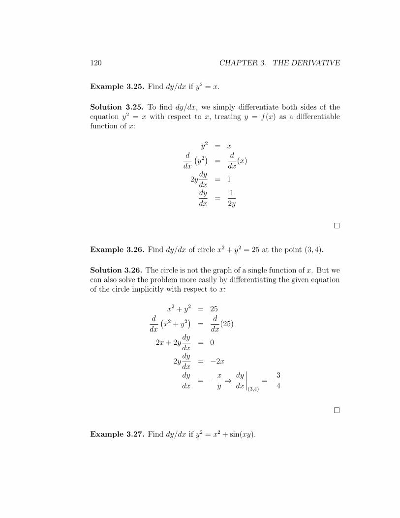
120 CHAPTER 3. THE DERIVATIVE
Example 3.25. Find dy/dx if y2 = x.
Solution 3.25. To find dy/dx, we simply differentiate both sides of theequation y2 = x with respect to x, treating y = f(x) as a differentiablefunction of x:
y2 = xd
dx
(y2)
=d
dx(x)
2ydy
dx= 1
dy
dx=
1
2y
�
Example 3.26. Find dy/dx of circle x2 + y2 = 25 at the point (3, 4).
Solution 3.26. The circle is not the graph of a single function of x. But wecan also solve the problem more easily by differentiating the given equationof the circle implicitly with respect to x:
x2 + y2 = 25d
dx
(x2 + y2
)=
d
dx(25)
2x+ 2ydy
dx= 0
2ydy
dx= −2x
dy
dx= −x
y⇒ dy
dx
∣∣∣∣(3,4)
= −3
4
�
Example 3.27. Find dy/dx if y2 = x2 + sin(xy).
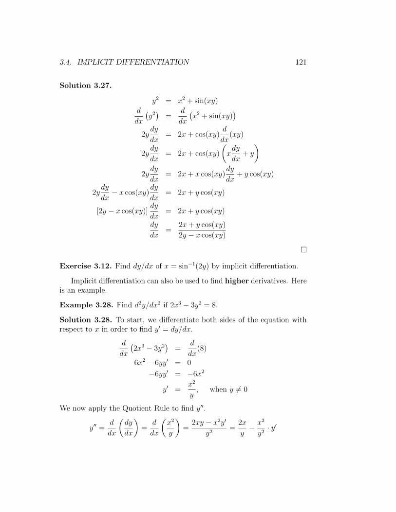
3.4. IMPLICIT DIFFERENTIATION 121
Solution 3.27.
y2 = x2 + sin(xy)
d
dx
(y2)
=d
dx
(x2 + sin(xy)
)2ydy
dx= 2x+ cos(xy)
d
dx(xy)
2ydy
dx= 2x+ cos(xy)
(xdy
dx+ y
)2ydy
dx= 2x+ x cos(xy)
dy
dx+ y cos(xy)
2ydy
dx− x cos(xy)
dy
dx= 2x+ y cos(xy)
[2y − x cos(xy)]dy
dx= 2x+ y cos(xy)
dy
dx=
2x+ y cos(xy)
2y − x cos(xy)
�
Exercise 3.12. Find dy/dx of x = sin−1(2y) by implicit differentiation.
Implicit differentiation can also be used to find higher derivatives. Hereis an example.
Example 3.28. Find d2y/dx2 if 2x3 − 3y2 = 8.
Solution 3.28. To start, we differentiate both sides of the equation withrespect to x in order to find y′ = dy/dx.
d
dx
(2x3 − 3y2
)=
d
dx(8)
6x2 − 6yy′ = 0
−6yy′ = −6x2
y′ =x2
y, when y 6= 0
We now apply the Quotient Rule to find y′′.
y′′ =d
dx
(dy
dx
)=
d
dx
(x2
y
)=
2xy − x2y′
y2=
2x
y− x2
y2· y′

122 CHAPTER 3. THE DERIVATIVE
Finally, we substitute y′ = x2/y to express y′′ in terms of x and y.
y′′ =2x
y− x2
y2x2
y2=
2x
y− x4
y3, when y 6= 0
�
Exercise 3.13. Find d2y/dx2 of x3 +y3 = 16 at the point (2, 2) by implicitdifferentiation.
The calculation of derivatives of complicated functions involving prod-ucts, quotients, or powers can often be simplified by taking logarithms. Themethod used in the following example is called logarithmic differentia-tion.
Example 3.29. Differentiate
y = x√x
Solution 3.29. Using logarithmic differentiation, we have
ln y = ln(x√x)
=√x lnx
d
dx(ln y) =
d
dx
(√x lnx
)y′
y=√x · 1
x+ lnx · 1
2√x
y′ = y
(1√x
+lnx
2√x
)= x
√x
(2 + ln x
2√x
)Exercise 3.14. Find dy/dx if y = (sinx)x.
3.5 Tangent Line
The problem of finding the tangent line to a curve involve calculating aderivative. If a curve C has equation y = f(x) and we want to find thetangent line to C at the point P (a, f(a)), then we consider a nearby pointQ(x, f(x)), where x 6= a, and compute the slope of the secant line PQ:
mPQ =f(x)− f(a)
x− a

3.5. TANGENT LINE 123
Then we let Q approach P along the curve C by letting x approach a. IfmPQ approaches a number m, then we define the tangent t to be the linethrough P with slope m. See Figure 3.3.
Figure 3.3:
Definition 3.5.1. The tangent line to the curve y = f(x) at the point(a, f(a)) is the line through the point with slope
m = limx→a
f(x)− f(a)
x− a= f ′(a)
provided that this limit exists.
Example 3.30. Find an equation of the tangent line to the parabola f(x) =x2 at the point with x−coordinate is x = 1.
Solution 3.30. Here, the tangent point is
(1, f(1)) =(1, 12
)= (1, 1)
Since f ′(x) = 2x then the slope is m = f ′(1) = 2 × 1 = 2. Using thepoint−slope form of the equation of a line, we find the equation of thetangent line at P (1, 1) as follows.
y − y0 = m (x− x0)y − 1 = 2(x− 1)
y = 2x− 1
�

124 CHAPTER 3. THE DERIVATIVE
Example 3.31. Find an equation of the tangent line to the hyperbolag(x) = 3/x at the point (3, 1).
Solution 3.31. Since f ′(x) = −3/x2, then the slope of the tangent at (3, 1)is
m = f ′(3) =−3
9= −1
3
Therefore an equation of the tangent at the point (3, 1) is
y − y0 = m (x− x0)
y − 1 = −1
3(x− 3)
y = −1
3x+ 2
�
Exercise 3.15. Find equations of the tangent line to the curve f(t) =t4 + 2et at the point (0, 2).
Example 3.32. Find equations of the tangent line to the curve f(x) =sin(sinx) at the point with x−coordinate is x = π.
Solution 3.32. Here, the tangent point is
(π, f(π)) = (π, sin(sinπ)) = (π, sin 0) = (π, 0)
Since f ′(x) = cos(sin x) cosx (by using Chain Rule), then the slope is
m = f ′(π) = cos(sin π) cosπ = cos(0)×−1 = 1×−1 = −1
Using the point−slope form of the equation of a line, we find the equationof the tangent line at P (π, 0) as follows.
y − y0 = m (x− x0)y − 0 = −1(x− π)
y = −x+ π
�

3.5. TANGENT LINE 125
Exercise 3.16. Find equations of the tangent line to the curve g(x) =(1 + 2x)10 at the point with x−coordinate is x = 0.
Example 3.33.
1. Find y′ if x3 + y3 = 6xy.
2. Find the tangent to x3 + y3 = 6xy at the point (3, 3).
3. At what points in the first quadrant is the tangent line horizontal?
Solution 3.33. 1. Differentiating both sides of x3 + y3 = 6xy with re-spect to x, regarding y as a function of x, and using the Chain Ruleon the term y3 and the Product Rule on the term 6xy, we get
3x2 + 3y2y′ = 6xy′ + 6y
y2y′ − 2xy′ = 2y − x2(y2 − 2x
)y′ = 2y − x2
y′ =2y − x2
y2 − 2x
2. When x = y = 3,
y′ =2× 3− 32
32 − 2× 3= −1
this is a reasonable value for the slope at (3, 3). So, an equation ofthe tangent to the curve at (3, 3) is
y − y0 = m (x− x0)y − 3 = −1(x− 3)
y = −x+ 6
3. The tangent line is horizontal if y′ = 0. Using the expression for y′
from part the first part, we see that y′ = 0 when 2y−x2 = 0 (providedthat y2 − 2x 6= 0). Substituting y = 1
2x2 in the equation of the curve,
we get
x3 +
(1
2x2)3
= 6x
(1
2x2)

126 CHAPTER 3. THE DERIVATIVE
which simplifies to x6 = 16x3. Now, solve the last equation:
x6 = 16x3
x6 − 16x3 = 0
x3(x3 − 16
)= 0
x3 = 0⇒ x = 0
x3 − 16 = 0⇒ x = 161/3
If x = 0 then y = 0, and if x = 161/3 = 24/3 then
y =1
2
(24/3
)2= 25/3
Thus the tangent is horizontal at (0, 0) and at(24/3, 25/3
).
�
Exercise 3.17. The curve with equation y2 = 5x4−x2 is called a kampyleof Eudoxus. Find an equation of the tangent line to this curve at the point(1, 2).
Chapter 4
Applications of Differentiation
This chapter studies some of the important applications of derivatives. Welearn how derivatives are used to find extreme values of functions, to de-termine and analyze the shapes of graphs, to calculate limits of fractionswhose numerators and denominators both approach zero or infinity, and tofind numerically where a function equals zero.
4.1 Indeterminate Forms and L’Hospital’s
Rule
John Bernoulli discovered a rule for calculating limits of fractions whosenumerators and denominators both approach zero or +∞. The rule isknown today as l’Hospital’s Rule, after Guillaume de l’Hospital. He was aFrench nobleman who wrote the first introductory differential calculus text,where the rule first appeared in print.
Indeterminate Form 0/0,∞/∞ If the functions f(x) and g(x) are bothzero or both ±∞ at x = a then
limx→a
f(x)
g(x)
cannot be found by substituting x = a. The substitution produces0/0 or ∞/∞, a meaningless expressions (indeterminate forms),that we cannot evaluate. Sometimes, but not always, limits that lead
127

128 CHAPTER 4. APPLICATIONS OF DIFFERENTIATION
to indeterminate forms may be found by cancelation, rearrangementof terms, or other algebraic manipulations. L’Hospital’s Rule enablesus to draw on our success with derivatives to evaluate limits thatotherwise lead to indeterminate forms.
Theorem 4.1.1. Suppose f and g are differentiable and g′(x) 6= 0 onan open interval I that contains a (except possibly at a). Suppose that
limx→a
f(x)
g(x)=
0
0or
±∞±∞
(In other words, we have an indeterminate form of type 0/0 or∞/∞.)Then
limx→a
f(x)
g(x)= lim
x→a
f ′(x)
g′(x)
if the limit on the right side exists or ±∞.
- L’Hospital’s Rule says that the limit of a quotient of functions isequal to the limit of the quotient of their derivatives, providedthat the given conditions are satisfied. It is especially importantto verify the conditions regarding the limits of and before usingL’Hospital’s Rule.
- L’Hospital’s Rule is also valid for one-sided limits and for limitsat infinity or negative infinity.
Example 4.1. Find
limx→1
lnx
x− 1
Solution 4.1. Since limx→1 lnx = 0 and limx→1(x− 1) = 0, then wecan apply L’Hospital’s Rule:
limx→1
lnx
x− 1= lim
x→1
ddx
(lnx)ddx
(x− 1)= lim
x→1
1/x
1= lim
x→1
1
x= 1
�
Example 4.2. Calculate
limx→∞
ex
x2

4.1. INDETERMINATE FORMS AND L’HOSPITAL’S RULE 129
Solution 4.2. We have limx→∞ ex = ∞ and limx→∞ x
2 = ∞, soL’Hospital’s Rule gives:
limx→∞
ex
x2= lim
x→∞
ddx
(ex)ddx
(x2)= lim
x→∞
ex
2x
Since ex → ∞ and 2x → ∞ as x → ∞, the limit on the right sideis also indeterminate, but a second application of L’Hospital’s Rulegives
limx→∞
ex
x2= lim
x→∞
ex
2x= lim
x→∞
ex
2=∞
�
Example 4.3. Calculate
limx→∞
lnx3√x
Solution 4.3. Since limx→∞ lnx = ∞ and limx→∞3√x = ∞ as x →
∞, L’Hospital’s Rule applies:
limx→∞
lnx3√x
= limx→∞
1/x13x−2/3
Notice that the limit on the right side is now indeterminate of type00. But instead of applying L’Hospital’s Rule a second time as we did
in the previous example, we simplify the expression and see that asecond application is unnecessary:
limx→∞
lnx3√x
= limx→∞
1/x13x−2/3
= limx→∞
33√x
= 0
�
Example 4.4. Find
limx→0
tanx− xx3

130 CHAPTER 4. APPLICATIONS OF DIFFERENTIATION
Solution 4.4. Noting that both tanx−x→ 0 and x3 → 0 as x→ 0,we use L’Hospital’s Rule:
limx→0
tanx− xx3
= limx→0
sec2 x− 1
3x2
Since the limit on the right side is still indeterminate of type 00, we
apply L’Hospital’s Rule again:
limx→0
tanx− xx3
= limx→0
sec2 x− 1
3x2
= limx→0
2 sec2 x tanx
6x
=2
6× lim
x→0sec2 x× lim
x→0
tanx
x
=1
3× 1× 1 =
1
1
�
Exercise 4.1. Find the limit.
(1) limt→0
et − 1
t3
(2) limt→∞
ln (ln t)
t
(3) limt→0
sin−1 t
t
(4) limt→∞
sinh t
et
Indeterminate Products 0 · ±∞ If limx→a f(x) = 0 and limx→a g(x) =±∞, then it is not clear what the value of limx→a [f(x)g(x)], if any,will be. There is a struggle between f and g. If f wins, the answerwill be 0; if g wins, the answer will be ±∞. Or there may be acompromise where the answer is a finite nonzero number. This kindof limit is called an indeterminate form of type 0 · ∞. We candeal with it by writing the product as a quotient:
fg =f
1/gor fg =
g
1/f
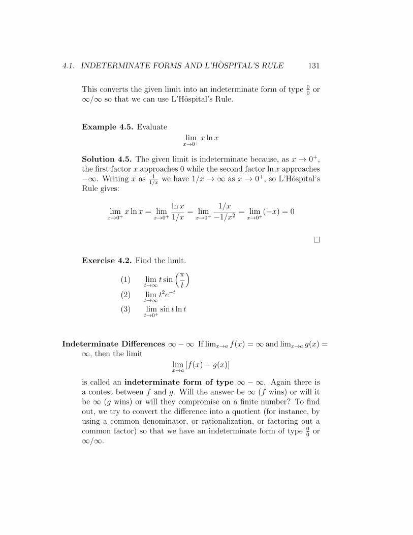
4.1. INDETERMINATE FORMS AND L’HOSPITAL’S RULE 131
This converts the given limit into an indeterminate form of type 00
or∞/∞ so that we can use L’Hospital’s Rule.
Example 4.5. Evaluate
limx→0+
x lnx
Solution 4.5. The given limit is indeterminate because, as x→ 0+,the first factor x approaches 0 while the second factor lnx approaches−∞. Writing x as 1
1/xwe have 1/x→∞ as x→ 0+, so L’Hospital’s
Rule gives:
limx→0+
x lnx = limx→0+
lnx
1/x= lim
x→0+
1/x
−1/x2= lim
x→0+(−x) = 0
�
Exercise 4.2. Find the limit.
(1) limt→∞
t sin(πt
)(2) lim
t→∞t2e−t
(3) limt→0+
sin t ln t
Indeterminate Differences ∞−∞ If limx→a f(x) =∞ and limx→a g(x) =∞, then the limit
limx→a
[f(x)− g(x)]
is called an indeterminate form of type ∞−∞. Again there isa contest between f and g. Will the answer be ∞ (f wins) or will itbe ∞ (g wins) or will they compromise on a finite number? To findout, we try to convert the difference into a quotient (for instance, byusing a common denominator, or rationalization, or factoring out acommon factor) so that we have an indeterminate form of type 0
0or
∞/∞.

132 CHAPTER 4. APPLICATIONS OF DIFFERENTIATION
Example 4.6. Evaluate
limx→(π/2)−
(secx− tanx)
Solution 4.6. First notice that sec x → ∞ and tanx → ∞ asx → (π/2)−, so the limit is indeterminate. Here we use a commondenominator:
limx→(π/2)−
(secx− tanx) = limx→(π/2)−
(1
cosx− sinx
cosx
)= lim
x→(π/2)−
1− sinx
cosx
= limx→(π/2)−
− cosx
− sinx= 0
�
Exercise 4.3. Find the limit.
(1) limt→∞
(√t2 + 1− t
)(2) lim
t→∞
(te1/t − t
)(3) lim
t→∞(t− ln t)
Indeterminate Powers 00,∞0,1∞ These several indeterminate forms arisefrom the limit
limx→a
[f(x)]g(x)
Each of these three cases can be treated by writing the function as anexponential:
[f(x)]g(x) = eg(x) ln f(x)
and then
limx→a
[f(x)]g(x) = elimx→a g(x) ln f(x)
where the indeterminate product g(x) ln f(x) is of type 0 · ∞.
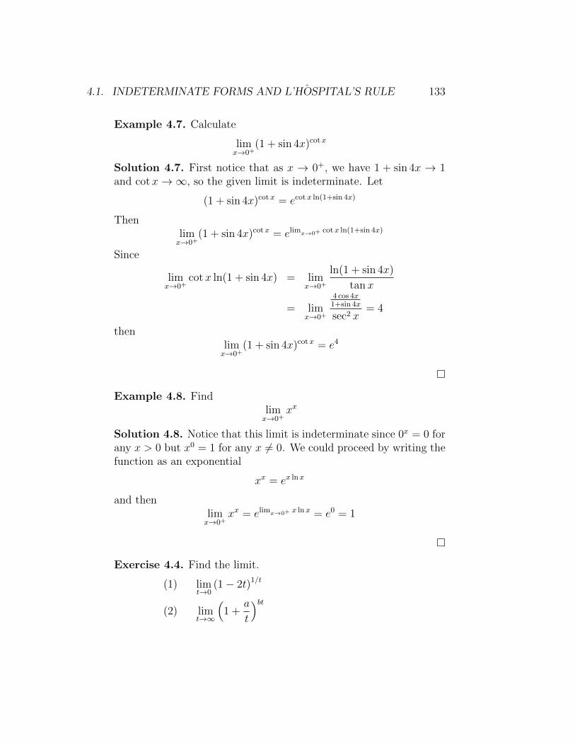
4.1. INDETERMINATE FORMS AND L’HOSPITAL’S RULE 133
Example 4.7. Calculate
limx→0+
(1 + sin 4x)cotx
Solution 4.7. First notice that as x → 0+, we have 1 + sin 4x → 1and cotx→∞, so the given limit is indeterminate. Let
(1 + sin 4x)cotx = ecotx ln(1+sin 4x)
Thenlimx→0+
(1 + sin 4x)cotx = elimx→0+ cotx ln(1+sin 4x)
Since
limx→0+
cotx ln(1 + sin 4x) = limx→0+
ln(1 + sin 4x)
tanx
= limx→0+
4 cos 4x1+sin 4x
sec2 x= 4
thenlimx→0+
(1 + sin 4x)cotx = e4
�
Example 4.8. Findlimx→0+
xx
Solution 4.8. Notice that this limit is indeterminate since 0x = 0 forany x > 0 but x0 = 1 for any x 6= 0. We could proceed by writing thefunction as an exponential
xx = ex lnx
and thenlimx→0+
xx = elimx→0+ x lnx = e0 = 1
�
Exercise 4.4. Find the limit.
(1) limt→0
(1− 2t)1/t
(2) limt→∞
(1 +
a
t
)bt
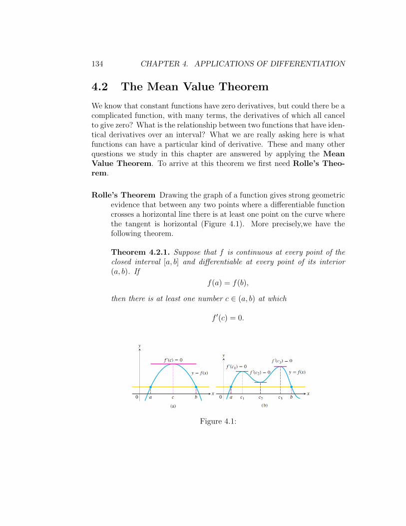
134 CHAPTER 4. APPLICATIONS OF DIFFERENTIATION
4.2 The Mean Value Theorem
We know that constant functions have zero derivatives, but could there be acomplicated function, with many terms, the derivatives of which all cancelto give zero? What is the relationship between two functions that have iden-tical derivatives over an interval? What we are really asking here is whatfunctions can have a particular kind of derivative. These and many otherquestions we study in this chapter are answered by applying the MeanValue Theorem. To arrive at this theorem we first need Rolle’s Theo-rem.
Rolle’s Theorem Drawing the graph of a function gives strong geometricevidence that between any two points where a differentiable functioncrosses a horizontal line there is at least one point on the curve wherethe tangent is horizontal (Figure 4.1). More precisely,we have thefollowing theorem.
Theorem 4.2.1. Suppose that f is continuous at every point of theclosed interval [a, b] and differentiable at every point of its interior(a, b). If
f(a) = f(b),
then there is at least one number c ∈ (a, b) at which
f ′(c) = 0.
Figure 4.1:

4.2. THE MEAN VALUE THEOREM 135
Example 4.9. Verify that the function
f(x) =x3
3− 3x
satisfies the three hypotheses of Rolle’s Theorem on the interval [−3, 3].Then find all numbers c that satisfy the conclusion of Rolle’s Theorem.
Solution 4.9. First, you can see that f(−3) = 0 = f(3). Since f isa polynomial, it is differentiable on (−3, 3) and continuous on [−3, 3].Thus, by Rolle’s Theorem, there is a number c ∈ (−3, 3) such that
f ′(c) = 0
c2 − 3 = 0
c2 = 3
c = ±√
3 ∈ (−3, 3)
�
Exercise 4.5. Verify that the function
f(x) = cos 2t
satisfies the three hypotheses of Rolle’s Theorem on the interval[π8, 7π
8
].
Then find all numbers c that satisfy the conclusion of Rolle’s Theorem.
Mean Value Theorem The Mean Value Theorem, which was first statedby Joseph Louis Lagrange, is a slanted version of Rolle’s Theorem(Figure 4.2). There is a point where the tangent is parallel to chordAB.
Theorem 4.2.2. Suppose that f is continuous on a closed interval[a, b] and differentiable on the interval’s interior (a, b). Then there isat least one number c ∈ (a, b) at which
f ′(c) =f(b)− f(a)
b− a.
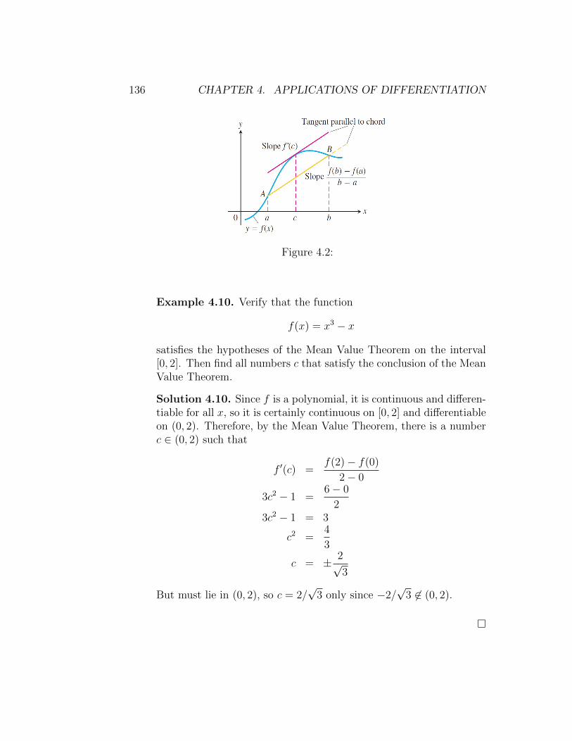
136 CHAPTER 4. APPLICATIONS OF DIFFERENTIATION
Figure 4.2:
Example 4.10. Verify that the function
f(x) = x3 − x
satisfies the hypotheses of the Mean Value Theorem on the interval[0, 2]. Then find all numbers c that satisfy the conclusion of the MeanValue Theorem.
Solution 4.10. Since f is a polynomial, it is continuous and differen-tiable for all x, so it is certainly continuous on [0, 2] and differentiableon (0, 2). Therefore, by the Mean Value Theorem, there is a numberc ∈ (0, 2) such that
f ′(c) =f(2)− f(0)
2− 0
3c2 − 1 =6− 0
23c2 − 1 = 3
c2 =4
3
c = ± 2√3
But must lie in (0, 2), so c = 2/√
3 only since −2/√
3 6∈ (0, 2).
�

4.2. THE MEAN VALUE THEOREM 137
Exercise 4.6. Verify that the function
f(x) = e−2x
satisfies the hypotheses of the Mean Value Theorem on the interval[0, 3]. Then find all numbers c that satisfy the conclusion of the MeanValue Theorem.
Example 4.11. Suppose that f(0) = −3 and f ′(x) ≤ 5 for all valuesof x. How large can f(2) possibly be?
Solution 4.11. We are given that f is differentiable (and thereforecontinuous) everywhere. In particular, we can apply the Mean ValueTheorem on the interval [0, 2]. There exists a number c ∈ (0, 2) suchthat
f ′(c) =f(2)− f(0)
2− 02f ′(c) = f(2)− (−3)
2f ′(c)− 3 = f(2)
We are given that f ′(x) ≤ 5 for all x, so in particular we know thatf ′(c) ≤ 5. Multiplying both sides of this inequality by 2, we have2f ′(c) ≤ 10, so
f(2) = 2f ′(c)− 3 ≤ 10− 3 = 7.
Thus, the largest possible value for f(2) is 7.
�
Exercise 4.7. If g(1) = 10 and g′(t) ≥ 2 for 1 ≤ t ≤ 4, how smallcan g(4) possibly be?
Mathematical Consequences At the beginning of the section, we askedwhat kind of function has a zero derivative over an interval. The firstcorollary of the Mean Value Theorem provides the answer.

138 CHAPTER 4. APPLICATIONS OF DIFFERENTIATION
Corollary 4.2.3. If f ′(x) = 0 at each point x of an open interval(a, b), then f(x) = C for all x ∈ (a, b), where C is a constant.
Example 4.12. Prove the identity tan−1 x+ cot−1 x = π/2.
Solution 4.12. Although calculus is not needed to prove this identity,the proof using calculus is quite simple. If f(x) = tan−1 x + cot−1 x,then
f ′(x) =1
1 + x2− 1
1 + x2= 0
for all values of x. Therefore f(x) = C, a constant. To determine thevalue of C, we put x = 1 because we can evaluate exactly. Then
C = f(1) = tan−1 1 + cot−1 1 =π
4+π
4=π
2.
Thus tan−1 x+ cot−1 x = π/2.
�
At the beginning of this section, we also asked about the relationshipbetween two functions that have identical derivatives over an inter-val. The next corollary tells us that their values on the interval havea constant difference.
Corollary 4.2.4. If f ′(x) = g′(x) at each point x in an open interval(a, b), then there exists a constant C such that f(x) = g(x) + C forall x ∈ (a, b). That is, f − g is a constant on (a, b).
Exercise 4.8. Prove the identity
2 sin−1 x = cos−1(1− 2x2
)for x ≥ 0

4.3. EXTREME VALUES OF FUNCTIONS 139
4.3 Extreme Values of Functions
This section shows how to locate and identify extreme values of a continuousfunction from its derivative. Once we can do this, we can solve a varietyof optimization problems in which we find the optimal (best) way to dosomething in a given situation.
Definition 4.3.1. Let f be a function with domain D. Then f has anabsolute maximum value on D at a point c if f(x) ≤ f(c) for all x ∈ Dand an absolute minimum value on D at c if f(x) ≥ f(c) for all x ∈ D.
Absolute maximum and minimum values are called absolute extrema(plural of the Latin extremum). Absolute extrema are also called globalextrema, to distinguish them from local extrema defined later in this sec-tion.
Illustration Example 4.1. For example, on the closed interval[−π
2, π2
]the function f(x) = cosx takes on an absolute maximum value of 1 (once)and an absolute minimum value of 0 (twice). On the same interval, thefunction g(x) = sinx takes on a maximum value of 1 and a minimum valueof −1 (Figure 4.3).
Figure 4.3:
Illustration Example 4.2. The absolute extrema of the following func-tions on their domains can be seen in Figure 4.4. Each function has the

140 CHAPTER 4. APPLICATIONS OF DIFFERENTIATION
same defining equation y = x2, but the domains vary. Notice that a func-tion might not have a maximum or minimum if the domain is unboundedor fails to contain an endpoint.
Function rule Domain D Absolute extrema on Dy = x2 (−∞,∞) No absolute maximum.
Absolute minimum of 0 at x = 0y = x2 [0, 2] Absolute maximum of 4 at x = 2
Absolute minimum of 0 at x = 0y = x2 (0, 2] Absolute maximum of 4 at x = 2
No absolute minimumy = x2 (0, 2) No absolute extrema
Figure 4.4:
The following theorem asserts that a function which is continuous atevery point of a closed interval [a, b] has an absolute maximum and anabsolute minimum value on the interval. We always look for these valueswhen we graph a function.
Theorem 4.3.1. If f is continuous on a closed interval [a, b], then f attainsboth an absolute maximum value M and an absolute minimum value m in[a, b]. That is, there are numbers x1 and x2 in [a, b] with f (x1) = m,f (x2) = M and m ≤ f(x) ≤M for every other x in [a, b].
Local (Relative) Extreme Values Figure 4.5 shows a graph with fivepoints where a function has extreme values on its domain [a, b]. Thefunction’s absolute minimum occurs at a even though at e the func-tion’s value is smaller than at any other point nearby. The curve rises

4.3. EXTREME VALUES OF FUNCTIONS 141
to the left and falls to the right around c, making f(c) a maximumlocally. The function attains its absolute maximum at d.
Figure 4.5:
Definition 4.3.2. A function f has a local maximum value at aninterior point c of its domain if
f(x) ≤ f(c) for all x in some open interval containing c
A function f has a local minimum value at an interior point c of itsdomain if
f(x) ≥ f(c) for all x in some open interval containing c
We can extend the definitions of local extrema to the endpoints ofintervals by defining f to have a local maximum or local minimumvalue at an endpoint c if the appropriate inequality holds for all x insome half-open interval in its domain containing c. In Figure 4.5, thefunction f has local maxima at c and d and local minima at a, e, andb. Local extrema are also called relative extrema.
An absolute maximum is also a local maximum. Being the largestvalue overall, it is also the largest value in its immediate neighbor-hood. Hence, a list of all local maxima will automatically include theabsolute maximum if there is one. Similarly, a list of all local minimawill include the absolute minimum if there is one.
The next theorem explains why we usually need to investigate only afew values to find a function’s extrema.
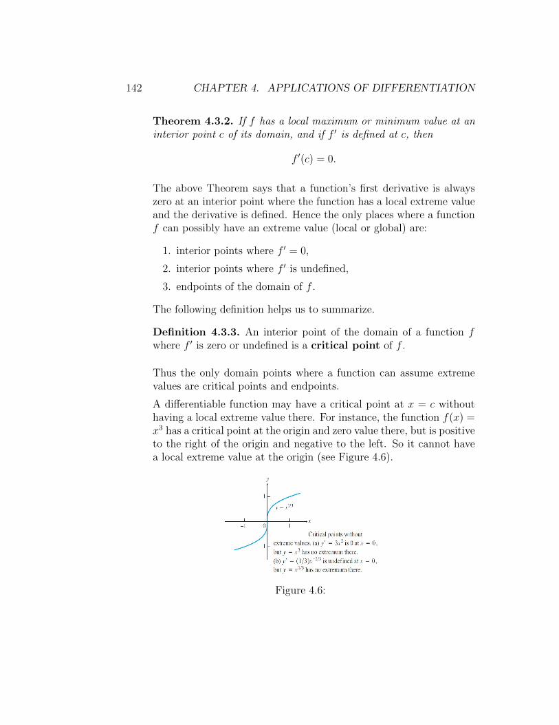
142 CHAPTER 4. APPLICATIONS OF DIFFERENTIATION
Theorem 4.3.2. If f has a local maximum or minimum value at aninterior point c of its domain, and if f ′ is defined at c, then
f ′(c) = 0.
The above Theorem says that a function’s first derivative is alwayszero at an interior point where the function has a local extreme valueand the derivative is defined. Hence the only places where a functionf can possibly have an extreme value (local or global) are:
1. interior points where f ′ = 0,
2. interior points where f ′ is undefined,
3. endpoints of the domain of f .
The following definition helps us to summarize.
Definition 4.3.3. An interior point of the domain of a function fwhere f ′ is zero or undefined is a critical point of f .
Thus the only domain points where a function can assume extremevalues are critical points and endpoints.
A differentiable function may have a critical point at x = c withouthaving a local extreme value there. For instance, the function f(x) =x3 has a critical point at the origin and zero value there, but is positiveto the right of the origin and negative to the left. So it cannot havea local extreme value at the origin (see Figure 4.6).
Figure 4.6:
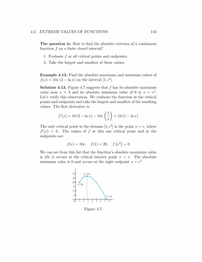
4.3. EXTREME VALUES OF FUNCTIONS 143
The question is: How to find the absolute extrema of a continuousfunction f on a finite closed interval?
1. Evaluate f at all critical points and endpoints.
2. Take the largest and smallest of these values.
Example 4.13. Find the absolute maximum and minimum values off(x) = 10x (2− lnx) on the interval [1, e2].
Solution 4.13. Figure 4.7 suggests that f has its absolute maximumvalue near x = 3 and its absolute minimum value of 0 at x = e2.Let’s verify this observation. We evaluate the function at the criticalpoints and endpoints and take the largest and smallest of the resultingvalues. The first derivative is
f ′(x) = 10 (2− lnx)− 10x
(1
x
)= 10 (1− lnx)
The only critical point in the domain [1, e2] is the point x = e, wheref ′(x) = 0. The values of f at this one critical point and at theendpoints are:
f(e) = 10e, f(1) = 20, f(e2)
= 0
We can see from this list that the function’s absolute maximum valueis 10e it occurs at the critical interior point x = e. The absoluteminimum value is 0 and occurs at the right endpoint x = e2.
Figure 4.7:

144 CHAPTER 4. APPLICATIONS OF DIFFERENTIATION
Example 4.14. Find the absolute maximum and minimum values off(x) = x2/3 on the interval [−2, 3].
Solution 4.14. We evaluate the function at the critical points andendpoints and take the largest and smallest of the resulting values.The first derivative
f ′(x) =2
3x−1/3 =
2
3 3√x
has no zeros but is undefined at the interior point x = 0. The valuesof f at this one critical point and at the endpoints are
f(0) = 0, f(−2) =3√
4, f(3) =3√
9
We can see from this list that the function’s absolute maximum valueis 3√
9 and it occurs at the right endpoint x = 3. The absolute min-imum value is 0, and it occurs at the interior point x = 0 where thegraph has a cusp (Figure 4.8).
Figure 4.8:
Exercise 4.9. Find the absolute maximum and minimum values ofg(t) = t2 on [−2, 1].
Example 4.15. If the function f(x) = x3 + ax2 + bx has the localminimum value −2
9
√3 at x = 1/
√3, what are the values of a and b.

4.3. EXTREME VALUES OF FUNCTIONS 145
Solution 4.15. Since f has the local minimum value −29
√3 at x =
1/√
3 then we know two things:
f
(1√3
)= −2
9
√3(
1√3
)3
+ a
(1√3
)2
+ b
(1√3
)= −2
9
√3
1
3√
3+a
3+
b√3
= −2
9
√3
1 + a√
3 + 3b = −2√3a+ 3b = −3 this is equation 1
and
f ′(
1√3
)= 0
3
(1√3
)2
+
(2a√
3
)+ b = 0
2a+√
3b = −√
3 this is equation 2
By solving equations 1 and 2 we obtain: a = 0 and b = −1.
�
Exercise 4.10. For what values of the numbers a and b does thefunction
g(t) = atebt2
have the maximum value g(2) = 1?
Exercise 4.11. Find the absolute maximum and minimum values ofeach function on the given interval.
1. g(t) = −1/t; −2 ≤ t ≤ −1
2. g(t) = 3√t; −1 ≤ t ≤ 8
3. g(t) = sin t; −π2≤ t ≤ 5π
6

146 CHAPTER 4. APPLICATIONS OF DIFFERENTIATION
4.4 Monotonic Functions
In sketching the graph of a differentiable function, it is useful to know whereit increases (rises from left to right) and where it decreases (falls fromleft to right) over an interval. This section gives a test to determine whereit increases and where it decreases. We also show how to test the criticalpoints of a function to identify whether local extreme values are present.
Increasing Functions and Decreasing Functions If the graph of a func-tion climbs or rises as you move from left to right, we say that thefunction is increasing. If the graph descends or falls as you move fromleft to right, the function is decreasing.
Definition 4.4.1. Let f be a function defined on an interval I andlet x1 and x2 be any two points in I.
1. If f (x2) > f (x1) whenever x1 < x2 then f is said to be increas-ing on I.
2. If f (x2) < f (x1) whenever x1 < x2 then f is said to be de-creasing on I.
It is important to realize that the definitions of increasing and de-creasing functions must be satisfied for every pair of points x1 andx2 in I with x1 < x2. Because we use the inequality < to comparethe function values, instead of it is sometimes said that f is strictlyincreasing or decreasing on I. The interval I may be finite (also calledbounded) or infinite (unbounded) and never consists of a single point.
As another corollary to the Mean Value Theorem, functions with pos-itive derivatives are increasing functions and functions with negativederivatives are decreasing functions. A function that is increasing ordecreasing on an interval is said to be monotonic on the interval.
Corollary 4.4.1. Suppose that f is continuous on [a, b] and differen-tiable on (a, b).
* If f ′(x) > 0 at each point x ∈ (a, b), then f is increasing on[a, b].
* If f ′(x) < 0 at each point x ∈ (a, b), then f is decreasing on[a, b].
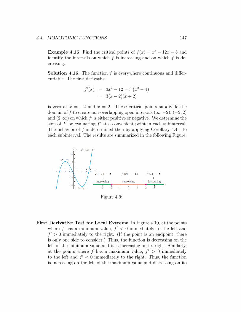
4.4. MONOTONIC FUNCTIONS 147
Example 4.16. Find the critical points of f(x) = x3 − 12x− 5 andidentify the intervals on which f is increasing and on which f is de-creasing.
Solution 4.16. The function f is everywhere continuous and differ-entiable. The first derivative
f ′(x) = 3x2 − 12 = 3(x2 − 4
)= 3(x− 2)(x+ 2)
is zero at x = −2 and x = 2. These critical points subdivide thedomain of f to create non-overlapping open intervals (∞,−2), (−2, 2)and (2,∞) on which f ′ is either positive or negative. We determine thesign of f ′ by evaluating f ′ at a convenient point in each subinterval.The behavior of f is determined then by applying Corollary 4.4.1 toeach subinterval. The results are summarized in the following Figure.
Figure 4.9:
First Derivative Test for Local Extrema In Figure 4.10, at the pointswhere f has a minimum value, f ′ < 0 immediately to the left andf ′ > 0 immediately to the right. (If the point is an endpoint, thereis only one side to consider.) Thus, the function is decreasing on theleft of the minimum value and it is increasing on its right. Similarly,at the points where f has a maximum value, f ′ > 0 immediatelyto the left and f ′ < 0 immediately to the right. Thus, the functionis increasing on the left of the maximum value and decreasing on its

148 CHAPTER 4. APPLICATIONS OF DIFFERENTIATION
Figure 4.10:
right. In summary, at a local extreme point, the sign of f ′(x) changes.
These observations lead to a test for the presence and nature of localextreme values of differentiable functions.
First Derivative Test for Local Extrema: Suppose that c is acritical point of a continuous function f , and that f is differentiableat every point in some interval containing c except possibly at c itself.Moving across this interval from left to right,
1. if f ′ changes from negative to positive at c, then f has a localminimum at c;
2. if f ′ changes from positive to negative at c, then f has a localmaximum at c;
3. if f ′ does not change sign at c (that is, is positive on both sidesof c or negative on both sides), then f has no local extremum atc.
Example 4.17. Find the critical points of
f(x) = x1/3(x− 4) = x4/3 − 4x1/3.
Identify the intervals on which f is increasing and decreasing. Findthe function’s local and absolute extreme values.
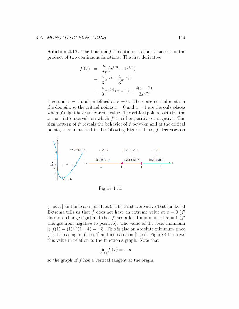
4.4. MONOTONIC FUNCTIONS 149
Solution 4.17. The function f is continuous at all x since it is theproduct of two continuous functions. The first derivative
f ′(x) =d
dx
(x4/3 − 4x1/3
)=
4
3x1/3 − 4
3x−2/3
=4
3x−2/3(x− 1) =
4(x− 1)
3x2/3
is zero at x = 1 and undefined at x = 0. There are no endpoints inthe domain, so the critical points x = 0 and x = 1 are the only placeswhere f might have an extreme value. The critical points partition thex−axis into intervals on which f ′ is either positive or negative. Thesign pattern of f ′ reveals the behavior of f between and at the criticalpoints, as summarized in the following Figure. Thus, f decreases on
Figure 4.11:
(−∞, 1] and increases on [1,∞). The First Derivative Test for LocalExtrema tells us that f does not have an extreme value at x = 0 (f ′
does not change sign) and that f has a local minimum at x = 1 (f ′
changes from negative to positive). The value of the local minimumis f(1) = (1)1/3(1− 4) = −3. This is also an absolute minimum sincef is decreasing on (−∞, 1] and increases on [1,∞). Figure 4.11 showsthis value in relation to the function’s graph. Note that
limx→0
f ′(x) = −∞
so the graph of f has a vertical tangent at the origin.

150 CHAPTER 4. APPLICATIONS OF DIFFERENTIATION
Example 4.18. Find the critical points of
f(x) =(x2 − 3
)ex.
Identify the intervals on which f is increasing and decreasing. Findthe function’s local and absolute extreme values.
Solution 4.18. The function f is continuous and differentiable forall real numbers, so the critical points occur only at the zeros of f ′.Using the Derivative Product Rule, we find the derivative
f ′(x) =(x2 − 3
) d
dxex + ex
d
dx
(x2 − 3
)=
(x2 − 3
)ex + ex(2x)
=(x2 + 2x− 3
)ex
Since ex is never zero, the first derivative is zero if and only if
x2 + 2x− 3 = 0
(x+ 3)(x− 1) = 0
The zeros x = −3 and x = 1 partition the x−axis into intervalsas follows. We can see from the Figure 4.12 that there is a local
Figure 4.12:
maximum at x = −3 and a local minimum at x = 1. The localminimum value is also an absolute minimum. There is no absolutemaximum. The function increases on (−∞,−3]
⋃[1,∞) and decreases
on [−3, 1]. Figure 4.12 also shows the graph.

4.5. CONCAVITY AND CURVE SKETCHING 151
Exercise 4.12. For each of the following functions: Find the open in-tervals on which the function is increasing and decreasing, and identifythe function’s local and absolute extreme values, if any, saying wherethey occur.
(1) g(t) = t− 6√t− 1
(2) g(t) = t ln t
Exercise 4.13. Show that g(t) = t− ln t is increasing for t > 1.
4.5 Concavity and Curve Sketching
We have seen how the first derivative tells us where a function is increasing,where it is decreasing, and whether a local maximum or local minimumoccurs at a critical point. In this section we see that the second deriva-tive gives us information about how the graph of a differentiable functionbends or turns. With this knowledge about the first and second derivatives,coupled with our previous understanding of symmetry and asymptotic be-havior, we can now draw an accurate graph of a function. By organizingall of these ideas into a coherent procedure, we give a method for sketchinggraphs and revealing visually the key features of functions. Identifying andknowing the locations of these features is of major importance in math-ematics and its applications to science and engineering, especially in thegraphical analysis and interpretation of data.
Concavity As you can see in Figure 4.13, the curve y = x3 rises as xincreases, but the portions defined on the intervals (∞, 0) and (0,∞)turn in different ways. As we approach the origin from the left alongthe curve, the curve turns to our right and falls below its tangents.The slopes of the tangents are decreasing on the interval (∞, 0). As wemove away from the origin along the curve to the right, the curve turnsto our left and rises above its tangents. The slopes of the tangents areincreasing on the interval (0,∞). This turning or bending behaviordefines the concavity of the curve.
Definition 4.5.1. The graph of a differentiable function y = f(x) is
1. concave up on an open interval I if f ′ is increasing on I;
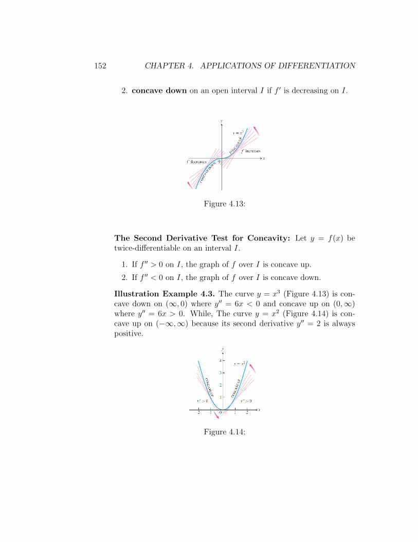
152 CHAPTER 4. APPLICATIONS OF DIFFERENTIATION
2. concave down on an open interval I if f ′ is decreasing on I.
Figure 4.13:
The Second Derivative Test for Concavity: Let y = f(x) betwice-differentiable on an interval I.
1. If f ′′ > 0 on I, the graph of f over I is concave up.
2. If f ′′ < 0 on I, the graph of f over I is concave down.
Illustration Example 4.3. The curve y = x3 (Figure 4.13) is con-cave down on (∞, 0) where y′′ = 6x < 0 and concave up on (0,∞)where y′′ = 6x > 0. While, The curve y = x2 (Figure 4.14) is con-cave up on (−∞,∞) because its second derivative y′′ = 2 is alwayspositive.
Figure 4.14:
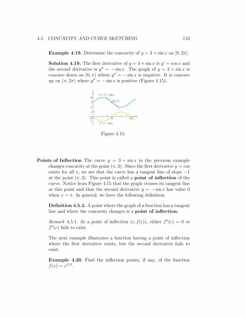
4.5. CONCAVITY AND CURVE SKETCHING 153
Example 4.19. Determine the concavity of y = 3 + sinx on [0, 2π].
Solution 4.19. The first derivative of y = 3 + sinx is y′ = cosx andthe second derivative is y′′ = − sinx. The graph of y = 3 + sin x isconcave down on (0, π) where y′′ = − sinx is negative. It is concaveup on (π, 2π) where y′′ = − sinx is positive (Figure 4.15).
Figure 4.15:
Points of Inflection The curve y = 3 + sinx in the previous examplechanges concavity at the point (π, 3). Since the first derivative y = cosexists for all x, we see that the curve has a tangent line of slope −1at the point (π, 3). This point is called a point of inflection of thecurve. Notice from Figure 4.15 that the graph crosses its tangent lineat this point and that the second derivative y = − sinx has value 0when x = π. In general, we have the following definition.
Definition 4.5.2. A point where the graph of a function has a tangentline and where the concavity changes is a point of inflection.
Remark 4.5.1. At a point of inflection (c, f(c)), either f ′′(c) = 0 orf ′′(c) fails to exist.
The next example illustrates a function having a point of inflectionwhere the first derivative exists, but the second derivative fails toexist.
Example 4.20. Find the inflection points, if any, of the functionf(x) = x5/3.

154 CHAPTER 4. APPLICATIONS OF DIFFERENTIATION
Solution 4.20. The graph of f(x) = x5/3 has a horizontal tangentat the origin because f ′(x) = 5
3x2/3 = 0 when x = 0. However, the
second derivative
f ′′(x) =d
dx
(5
3x2/3
)=
10
9x−1/3 =
10
9 3√x
fails to exist at x = 0. Nevertheless, f ′′(x) < 0 for x < 0 and f ′′(x) > 0for x > 0, so the second derivative changes sign at x = 0 and there isa point of inflection at the origin. The graph is shown in Figure 4.16.
Figure 4.16:
Here is an example showing that an inflection point need not occureven though both derivatives exist and f ′′ = 0.
Example 4.21. Find the inflection points, if any, of the functionf(x) = x4.
Solution 4.21. The curve y = x4 has no inflection point at x = 0(Figure 4.17). Even though the second derivative y′′ = 12x2 is zerothere, it does not change sign.
�
As our final illustration, we show a situation in which a point ofinflection occurs at a vertical tangent to the curve where neither thefirst nor the second derivative exists.
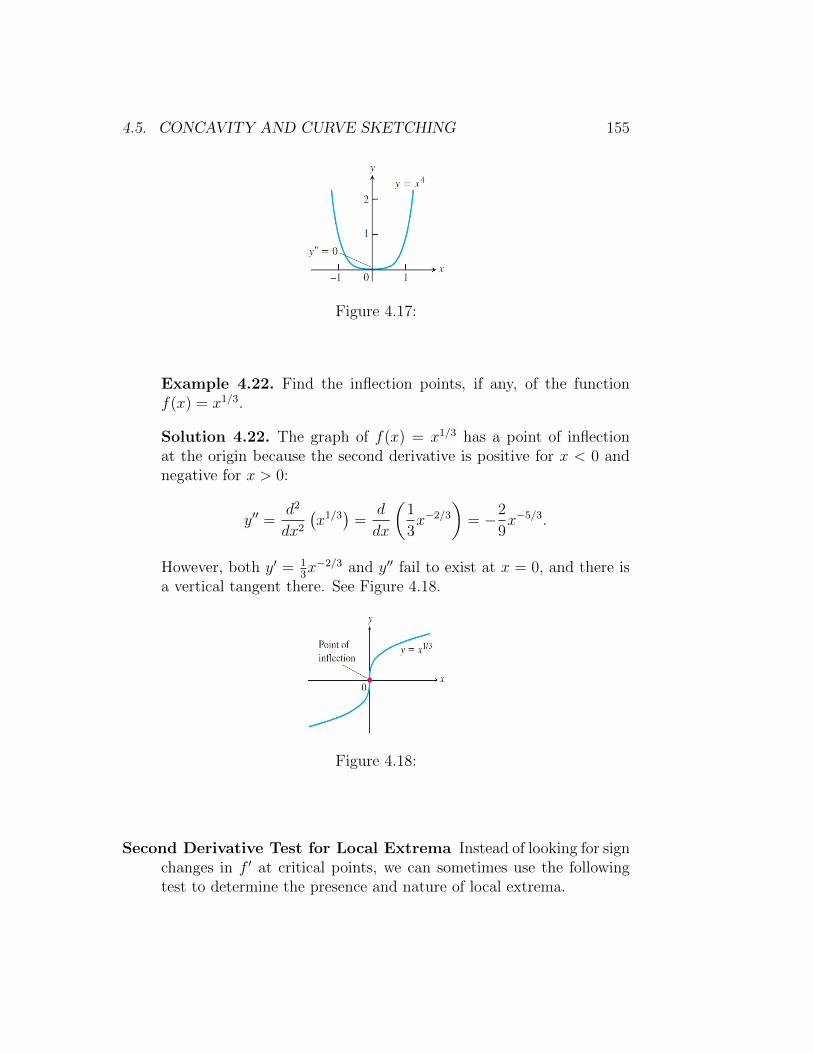
4.5. CONCAVITY AND CURVE SKETCHING 155
Figure 4.17:
Example 4.22. Find the inflection points, if any, of the functionf(x) = x1/3.
Solution 4.22. The graph of f(x) = x1/3 has a point of inflectionat the origin because the second derivative is positive for x < 0 andnegative for x > 0:
y′′ =d2
dx2(x1/3
)=
d
dx
(1
3x−2/3
)= −2
9x−5/3.
However, both y′ = 13x−2/3 and y′′ fail to exist at x = 0, and there is
a vertical tangent there. See Figure 4.18.
Figure 4.18:
Second Derivative Test for Local Extrema Instead of looking for signchanges in f ′ at critical points, we can sometimes use the followingtest to determine the presence and nature of local extrema.
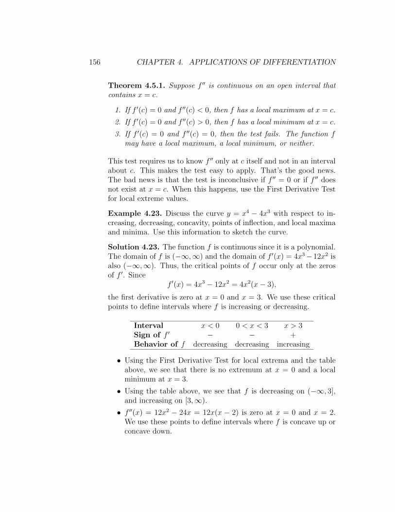
156 CHAPTER 4. APPLICATIONS OF DIFFERENTIATION
Theorem 4.5.1. Suppose f ′′ is continuous on an open interval thatcontains x = c.
1. If f ′(c) = 0 and f ′′(c) < 0, then f has a local maximum at x = c.
2. If f ′(c) = 0 and f ′′(c) > 0, then f has a local minimum at x = c.
3. If f ′(c) = 0 and f ′′(c) = 0, then the test fails. The function fmay have a local maximum, a local minimum, or neither.
This test requires us to know f ′′ only at c itself and not in an intervalabout c. This makes the test easy to apply. That’s the good news.The bad news is that the test is inconclusive if f ′′ = 0 or if f ′′ doesnot exist at x = c. When this happens, use the First Derivative Testfor local extreme values.
Example 4.23. Discuss the curve y = x4 − 4x3 with respect to in-creasing, decreasing, concavity, points of inflection, and local maximaand minima. Use this information to sketch the curve.
Solution 4.23. The function f is continuous since it is a polynomial.The domain of f is (−∞,∞) and the domain of f ′(x) = 4x3−12x2 isalso (−∞,∞). Thus, the critical points of f occur only at the zerosof f ′. Since
f ′(x) = 4x3 − 12x2 = 4x2(x− 3),
the first derivative is zero at x = 0 and x = 3. We use these criticalpoints to define intervals where f is increasing or decreasing.
Interval x < 0 0 < x < 3 x > 3Sign of f ′ − − +Behavior of f decreasing decreasing increasing
• Using the First Derivative Test for local extrema and the tableabove, we see that there is no extremum at x = 0 and a localminimum at x = 3.
• Using the table above, we see that f is decreasing on (−∞, 3],and increasing on [3,∞).
• f ′′(x) = 12x2 − 24x = 12x(x − 2) is zero at x = 0 and x = 2.We use these points to define intervals where f is concave up orconcave down.

4.5. CONCAVITY AND CURVE SKETCHING 157
Interval x < 0 0 < x < 2 x > 2Sign of f ′′ + − +Behavior of f concave up concave down concave up
We see that f is concave up on the intervals (∞, 0)⋃
(2,∞) andconcave down on (0, 2). The general shape of the curve is shownFigure 4.19.
Figure 4.19:
Exercise 4.14. Find the intervals of increasing, decreasing and con-cavity, the extremum points and the points of inflections, of each ofthe following functions. Use this information to sketch the curve.
(1) g(t) = tan−1 t (2) g(t) =4 + t2
2t
Exercise 4.15. The accompanying figure shows a portion of thegraph of a twice-differentiable function y = f(x). At each of thefive labeled points, classify y′ and y′′ as positive, negative, or zero.
Example 4.24. The graph of the derivative f ′ of a function f isshown in Figure 4.21. On what intervals is f increasing or decreasing,concave up or down? At what values of x does f have a extreme andinflection points?
Solution 4.24. Since f ′(x) > 0 on (1, 5), f is increasing on thisinterval. Since f ′(x) < 0 on (0, 1) and (5, 6), f is decreasing on these
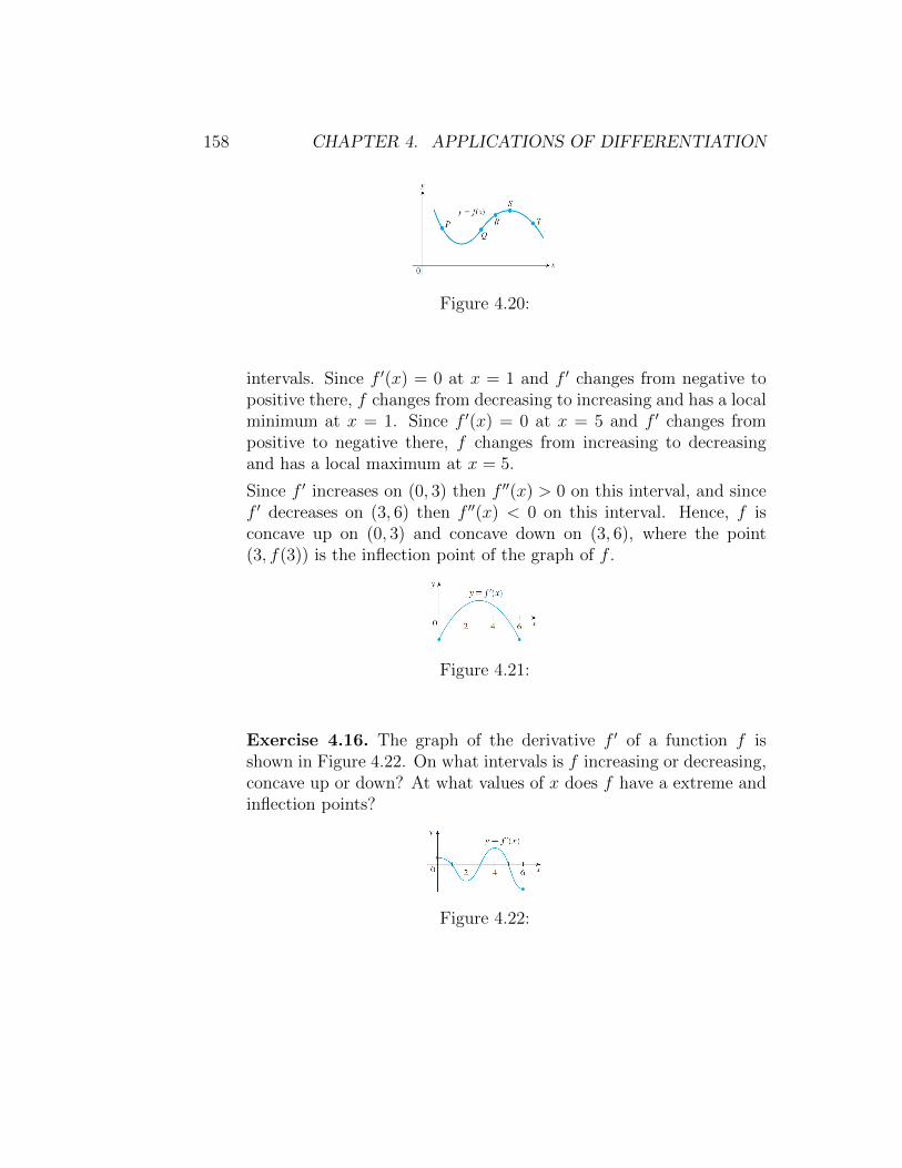
158 CHAPTER 4. APPLICATIONS OF DIFFERENTIATION
Figure 4.20:
intervals. Since f ′(x) = 0 at x = 1 and f ′ changes from negative topositive there, f changes from decreasing to increasing and has a localminimum at x = 1. Since f ′(x) = 0 at x = 5 and f ′ changes frompositive to negative there, f changes from increasing to decreasingand has a local maximum at x = 5.
Since f ′ increases on (0, 3) then f ′′(x) > 0 on this interval, and sincef ′ decreases on (3, 6) then f ′′(x) < 0 on this interval. Hence, f isconcave up on (0, 3) and concave down on (3, 6), where the point(3, f(3)) is the inflection point of the graph of f .
Figure 4.21:
Exercise 4.16. The graph of the derivative f ′ of a function f isshown in Figure 4.22. On what intervals is f increasing or decreasing,concave up or down? At what values of x does f have a extreme andinflection points?
Figure 4.22:

Chapter 5
Integration
The integral is of fundamental importance in statistics, the sciences, andengineering. As with the derivative, the integral also arises as a limit, thistime of increasingly fine approximations. We use it to calculate quanti-ties ranging from probabilities and averages to energy consumption andthe forces against a dams floodgates. In this chapter we focus on the inte-gral concept and its use in computing areas of various regions with curvedboundaries.
5.1 Antiderivatives
We have studied how to find the derivative of a function. However, manyproblems require that we recover a function from its known derivative. Moregenerally, starting with a function f , we want to find a function F whosederivative is f . If such a function F exists, it is called an antiderivativeof f . We will see next that antiderivatives are the link connecting the twomajor elements of calculus: derivatives and definite integrals.
Definition 5.1.1. A function F is an antiderivative of f on an intervalI if F ′(x) = f(x) for all x in I.
The process of recovering a function F (x) from its derivative f(x) iscalled anti-differentiation. We use capital letters such as F to represent anantiderivative of a function f , G to represent an antiderivative of g, and soforth.
159

160 CHAPTER 5. INTEGRATION
Example 5.1. Find an antiderivative for f(x) = 2x.
Solution 5.1. We need to think backward here: What function do we knowhas a derivative equal to 2x? It is not difficult to this question if we keepthe Power Rule in mind. In fact, if F (x) = x2, then F ′(x) = 2x = f(x).But the function G(x) = x2− 5 also satisfies G′(x) = 2x = f(x). Thereforeboth F and G are antiderivatives of f . Indeed, any function of the formH(x) = x2 + C, where C is a constant, is an antiderivative of f(x) = x2.
�
Theorem 5.1.1. If F is an antiderivative of f on an interval I, then themost general antiderivative of f on I is
F (x) + C
where C is an arbitrary constant.
Example 5.2. Find an antiderivative F of f(x) = 3x2 that satisfies F (1) =−1.
Solution 5.2. Since the derivative of x3 is 3x2, the general antiderivativeF (x) = x3 + C gives all the antiderivatives of f(x). The condition F (1) =−1 determines a specific value for C. Substituting x = 1 into F (x) gives
F (1) = 13 + C
−1 = 1 + C
C = −2
So, F (x) = x3 − 2 is the antiderivative satisfying F (1) = −1.
5.2 Indefinite Integrals
A special symbol is used to denote the collection of all antiderivatives of afunction f .
Definition 5.2.1. The collection of all antiderivatives of is called theindefinite integral of f with respect to x, and is denoted by∫
f(x)dx.

5.2. INDEFINITE INTEGRALS 161
The symbol∫
is an integral sign. The function f is the integrand of theintegral, and x is the variable of integration.
After the integral sign in the notation we just defined, the integrandfunction is always followed by a differential to indicate the variable of inte-gration. Using this notation, we have, for example:∫
2xdx = x2 + C∫cosx = sin x+ C
Exercise 5.1. Verify the formula∫tan−1 x
x2dx = lnx− 1
2ln(1 + x2
)− tan−1 x
x+ C.
In the following we list antiderivatives in the notation of indefinite in-tegrals. Each formula is true because the derivative of the function in theright appears in the left. In particular, these formulas are the rules ofintegration.
Rule 1 The first formula says that the integration of a constant times afunction is the constant times the integration of the function.∫
cf(x)dx = c
∫f(x)dx
Rule 2 The second formula says that the integration of a sum (difference)is the sum (difference) of the integrations.∫
[f(x)± g(x)] dx =
∫f(x)dx±
∫g(x)dx
Rule 3 The integration of constant functions is the constant itself times x.∫kdx = kx+ C where k is a constant
For example, ∫1
2dx =
1
2x+ C∫
πdx = πx+ C
162 CHAPTER 5. INTEGRATION
Rule 4 The integration of power functions is given by∫xndx =
xn+1
n+ 1+ C where n 6= 1
In general, ∫(ax+ b)ndx =
(ax+ b)n+1
a(n+ 1)+ C where n 6= 1
Example 5.3. Find the general indefinite integral∫ (x2 +
1
x2
)dx
Solution 5.3.∫ (x2 +
1
x2
)dx =
∫x2dx+
∫x−2dx
=1
3x3 +
1
−1x−1 + C
=1
3x3 − 1
x+ C
�
Example 5.4. Find the general indefinite integral∫(x− 1)(x+ 3)dx
Solution 5.4.∫(x− 1)(x+ 3)dx =
∫ (x2 + 2x− 3
)dx
=
∫x2dx+ 2
∫xdx−
∫3dx
=1
3x3 + 2× 1
2x2 − 3x+ C
=1
3x3 + x2 − 3x+ C
5.2. INDEFINITE INTEGRALS 163
Example 5.5. Find the general indefinite integral∫3√x2dx
Solution 5.5.∫3√x2dx =
∫x2/3dx =
1
5/3x5/3 + C
=3
5
3√x5 + C
�
Example 5.6. Find the general indefinite integral∫x2 − 3
√x
xdx
Solution 5.6.∫x2 − 3
√x
xdx =
∫ (x2
x− 3√x
x
)dx
=
∫ (x− 3x−1/2
)dx
=
∫xdx− 3
∫x−1/2dx
=1
2x2 − 3× 1
1/2x1/2 + C
=1
2x2 − 6
√x+ C
�
Example 5.7. Find the general indefinite integral∫(1− 2x)99dx
Solution 5.7.∫(1− 2x)99dx =
(1− 2x)100
−2× 100+ C = −(1− 2x)100
200+ C

164 CHAPTER 5. INTEGRATION
Rule 5 The fifth rule is the first rule we learn about the integration of thedivision of two functions.∫
1
xdx = ln |x|+ C
In general, ∫f ′(x)
f(x)dx = ln |f(x)|+ C
Example 5.8. Find the general indefinite integral∫ex
9 + exdx
Solution 5.8. Since ddx
(9 + ex) = ex, then∫ex
9 + exdx = ln |9 + ex|+ C
�
Example 5.9. Find the general indefinite integral∫x
1 + x2dx
Solution 5.9. Note ddx
(1 + x2) = 2x 6= x. So, multiply the integralby 2
2to obtain:∫
x
1 + x2dx =
2
2
∫x
1 + x2dx =
1
2
∫2x
1 + x2dx
=1
2ln∣∣1 + x2
∣∣+ C
�
Example 5.10. Find the general indefinite integral∫tanxdx

5.2. INDEFINITE INTEGRALS 165
Solution 5.10. To evaluate this integral, write tanx as sinx/ cosx.Thus, ∫
tanxdx =
∫sinx
cosxdx = −
∫− sinx
cosxdx
= − ln | cosx|+ C = ln | secx|+ C
�
Rule 6 The rules of integration of exponential functions are as follows.∫exdx = ex + C and
∫axdx =
ax
ln a+ C
In general,∫eαx+βdx =
1
αeαx+β + C and
∫aαx+βdx =
aαx+β
α ln a+ C
Example 5.11. Find the general indefinite integral∫28−6xdx
Solution 5.11. ∫28−6xdx = − 28−6x
6× ln 2+ C
�
Example 5.12. Find the general indefinite integral∫e2 lnxdx
Solution 5.12.∫e2 lnxdx =
∫eln(x
2)dx =
∫x2dx =
1
3x3 + C
�
166 CHAPTER 5. INTEGRATION
Rule 7 The following rules represent the rules of integrations of sometrigonometric functions.
(1)
∫sinxdx = − cosx+ C.∫sin(αx+ β)dx = −cos(αx+ β)
α+ C
(2)
∫cosxdx = sinx+ C∫cos(αx+ β)dx =
sin(αx+ β)
α+ C
(3)
∫sec2 xdx = tanx+ C∫sec2(αx+ β)dx =
tan(αx+ β)
α+ C
(4)
∫csc2 xdx = − cotx+ C∫csc2(αx+ β)dx = −cot(αx+ β)
α+ C
(5)
∫secx tanxdx = secx+ C∫sec(αx+ β) tan(αx+ β)dx =
sec(αx+ β)
α+ C
(6)
∫cscx cotxdx = − cscx+ C∫csc(αx+ β) cot(αx+ β)dx = −csc(αx+ β)
α+ C
Example 5.13. Find the general indefinite integral
∫secx(tanx+ cosx)dx
5.2. INDEFINITE INTEGRALS 167
Solution 5.13.∫secx(tanx+ cosx)dx =
∫secx tanxdx+
∫secx cosxdx
=
∫secx tanxdx+
∫1
cosx· cosxdx
=
∫secx tanxdx+
∫1dx
= sec x+ x+ C
�
Example 5.14. Find the general indefinite integral∫secxdx
Solution 5.14.∫secxdx =
∫secx · secx+ tanx
secx+ tanxdx
=
∫sec2 x+ secx tanx
secx+ tanxdx
= ln |secx+ tanx|+ C
�
Example 5.15. Find the general indefinite integral∫sin(3x− 10)dx
Solution 5.15.∫sin(3x− 10)dx = −1
3cos(3x− 10) + C
�
168 CHAPTER 5. INTEGRATION
Example 5.16. Find the general indefinite integral∫tan2 xdx
Solution 5.16.∫tan2 xdx =
∫ (sec2 x− 1
)dx
=
∫sec2 xdx−
∫1dx
= tanx− x+ C
�
Example 5.17. Find the general indefinite integral∫1
1 + sin xdx
Solution 5.17.∫1
1 + sin xdx =
∫1
1 + sin x· 1− sinx
1− sinxdx
=
∫1− sinx
1− sin2 xdx =
∫1− sinx
cos2 xdx
=
∫1
cos2 xdx−
∫sinx
cos2 xdx
=
∫1
cos2 xdx−
∫sinx
cosx· 1
cosxdx
=
∫sec2 xdx−
∫tanx sec dx
= tan x− secx+ C
�

5.2. INDEFINITE INTEGRALS 169
Rule 8 The integration rules of the main inverse trigonometric functionsare:
(1)
∫1
1 + x2dx = tan−1 x+ C∫
1
a+ bx2dx =
1√ab
tan−1
(√b
ax
)+ C
(2)
∫1√
1− x2dx = sin−1 x+ C∫
1√a− bx2
dx =1√b
sin−1
(√b
ax
)+ C
(3)
∫1
|x|√x2 − 1
dx = sec−1 x+ C
Example 5.18. Find the general indefinite integral∫1
25 + 4x2dx
Solution 5.18.∫1
25 + 4x2dx =
1√25× 4
tan−1
(√4
25x
)+ C
=1
10tan−1
(2
5x
)+ C
Example 5.19. Find the general indefinite integral∫1√
16− 9x2dx
Solution 5.19.∫1√
16− 9x2=
1√9
sin−1
(√9
16x
)+ C
=1
3sin−1
(3
4x
)+ C

170 CHAPTER 5. INTEGRATION
Exercise 5.2. Evaluate the general indefinite integral.
(1)
∫t13
(1 + t2
)2dt
(2)
∫t+ 1
t2 + 2t+ 5dt
(3)
∫et − e−t
et + e−tdt
(4)
∫csc tdt
(5)
∫cot tdt
(6)
∫sin 2t
sin tdt
(7)
∫1
1 + cos 2tdt
(8)
∫ [1
2t+ 5t
]dt
(9)
∫1 + t+ t2
1 + t2dt
5.3 Integration by Substitution
In this section we will study a technique, called substitution, that canoften be used to transform complicated integration problems into simplerones. The method of substitution can be motivated by examining the chainrule from the viewpoint of anti-differentiation. For this purpose, supposethat F is an antiderivative of f and that g is a differentiable function. Thechain rule implies that the derivative of F (g(x)) can be expressed as
d
dxF (g(x)) = F ′(g(x))× g′(x)
which we can write in integral form as∫F ′(g(x))g′(x)dx = F (g(x)) + C

5.3. INTEGRATION BY SUBSTITUTION 171
or since F is an antiderivative of f ,∫f(g(x))g′(x)dx = F (g(x)) + C (5.3.1)
For our purposes it will be useful to let u = g(x) and to write du/dx = g′(x)in the differential form du = g′(x)dx. With this notation, equation 5.3.1can be expressed as ∫
f(u)du = F (u) + C (5.3.2)
The process of evaluating an integral of form 5.3.1 by converting it intoform 5.3.2 with the substitution
u = g(x) and du = g′(x)dx
is called the method of u−substitution. Here our emphasis is not onthe interpretation of the expression du = g′(x)dx. Rather, the differentialnotation serves primarily as a useful bookkeeping device for the method ofu−substitution. The following example illustrates how the method works.
Example 5.20. Evaluate ∫2x(x2 + 1
)50dx
Solution 5.20. If we let u = x2 + 1, then du/dx = 2x, which implies thatdu = 2xdx. Thus, the given integral can be written as∫
2x(x2 + 1
)50dx =
∫u50du =
u51
51+ C =
(x2 + 1)51
51+ C
�
Example 5.21. Evaluate ∫sin2 x cosxdx
Solution 5.21. If we let u = sinx, then du/dx = cos x, so du = cos xdx.Thus, ∫
sin2 x cosxdx =
∫u2du =
u3
3+ C =
sin3 x
3+ C
172 CHAPTER 5. INTEGRATION
Example 5.22. Evaluate ∫e√x
√xdx
Solution 5.22. If we let u =√x, then
du
dx=
1
2√x, so du =
1
2√xdx or 2du =
1√xdx
Thus. ∫e√x
√xdx =
∫2eudu = 2eu + C = 2e
√x + C
�
Example 5.23. Evaluate ∫x4
3√
3− 5x5dx
Solution 5.23. If we let u = 3− 5x5, then
du
dx= −25x4, so du = −25x4dx or − 1
25du = x4dx
Thus. ∫x4
3√
3− 5x5dx =
∫− 1
253√udu = − 1
25
∫u
13du
= − 1
25× 3
4u
43 + C
= − 3
100
(3− 5x5
) 43 + C
�
Example 5.24. Evaluate ∫ex√
1− e2xdx
5.3. INTEGRATION BY SUBSTITUTION 173
Solution 5.24. Substituting u = ex and du = exdx yields
∫ex√
1− e2xdx =
∫1√
1− u2du = sin−1 u+ C = sin−1 (ex) + C
�
The method of substitution is relatively straightforward, provided theintegrand contains an easily recognized composition f(g(x)) and the re-mainder of the integrand is a constant multiple of g′(x). If this is not thecase, the method may still apply but may require more computation.
Example 5.25. Evaluate
∫x2√x− 1dx
Solution 5.25. The composition√x− 1 suggests the substitution u = x−1
so that du = dx. From the equality u = x− 1 we have
x2 = (u+ 1)2 = u2 + 2u+ 1
so that∫x2√x− 1 =
∫ (u2 + 2u+ 1
)√udu =
∫ (u5/2 + 2u3/2 + u1/2
)du
=2
7u7/2 + 2× 2
5u5/2 +
2
3u3/2 + C
=2
7(x− 1)7/2 +
4
5(x− 1)5/2 +
2
3(x− 1)3/2 + C
�
174 CHAPTER 5. INTEGRATION
Exercise 5.3. Evaluate the integrals using appropriate substitutions.
(1)
∫t3√
5 + t4dt
(2)
∫sin(1/t)
3t2dt
(3)
∫esin t cos tdt
(4)
∫t
1 + t4dt
(5)
∫ √etdt
(6)
∫(ln t)2
tdt
(7)
∫t√t− 1dt
(8)
∫1
t ln tdt
(9)
∫(tan−1 t)
2
1 + t2dt
(10)
∫1
t2 + 2t+ 5dt
(11)
∫1
t+√tdt
(12)
∫sin(2t)
1 + cos2 tdt
(13)
∫(t− 1)5
t7dt
(14)
∫tan t ln(cos t)dt
(15)
∫1
tsin(
ln√t)dt
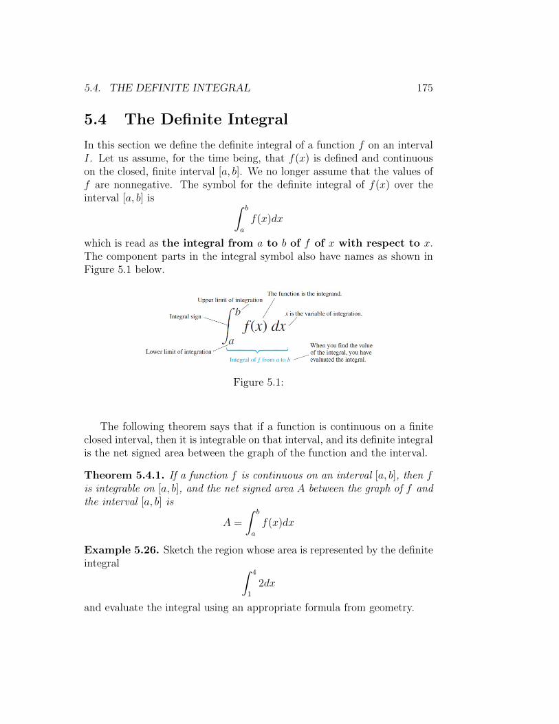
5.4. THE DEFINITE INTEGRAL 175
5.4 The Definite Integral
In this section we define the definite integral of a function f on an intervalI. Let us assume, for the time being, that f(x) is defined and continuouson the closed, finite interval [a, b]. We no longer assume that the values off are nonnegative. The symbol for the definite integral of f(x) over theinterval [a, b] is ∫ b
a
f(x)dx
which is read as the integral from a to b of f of x with respect to x.The component parts in the integral symbol also have names as shown inFigure 5.1 below.
Figure 5.1:
The following theorem says that if a function is continuous on a finiteclosed interval, then it is integrable on that interval, and its definite integralis the net signed area between the graph of the function and the interval.
Theorem 5.4.1. If a function f is continuous on an interval [a, b], then fis integrable on [a, b], and the net signed area A between the graph of f andthe interval [a, b] is
A =
∫ b
a
f(x)dx
Example 5.26. Sketch the region whose area is represented by the definiteintegral ∫ 4
1
2dx
and evaluate the integral using an appropriate formula from geometry.
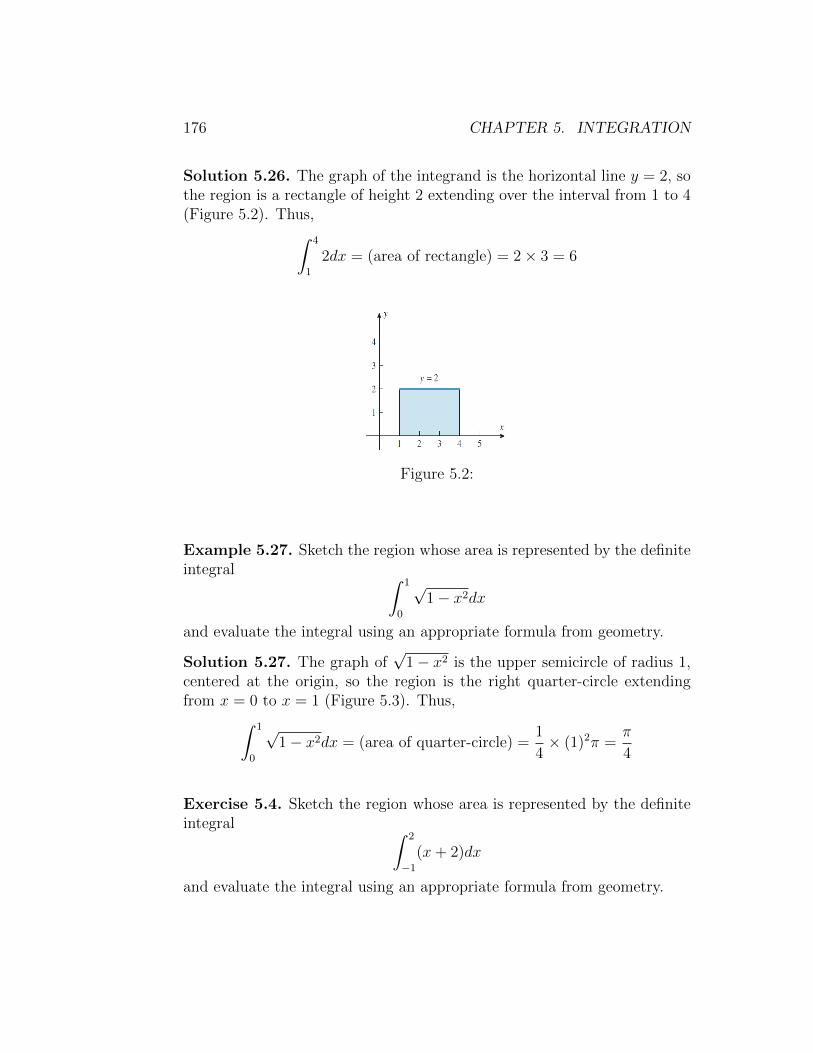
176 CHAPTER 5. INTEGRATION
Solution 5.26. The graph of the integrand is the horizontal line y = 2, sothe region is a rectangle of height 2 extending over the interval from 1 to 4(Figure 5.2). Thus,∫ 4
1
2dx = (area of rectangle) = 2× 3 = 6
Figure 5.2:
Example 5.27. Sketch the region whose area is represented by the definiteintegral ∫ 1
0
√1− x2dx
and evaluate the integral using an appropriate formula from geometry.
Solution 5.27. The graph of√
1− x2 is the upper semicircle of radius 1,centered at the origin, so the region is the right quarter-circle extendingfrom x = 0 to x = 1 (Figure 5.3). Thus,∫ 1
0
√1− x2dx = (area of quarter-circle) =
1
4× (1)2π =
π
4
Exercise 5.4. Sketch the region whose area is represented by the definiteintegral ∫ 2
−1(x+ 2)dx
and evaluate the integral using an appropriate formula from geometry.
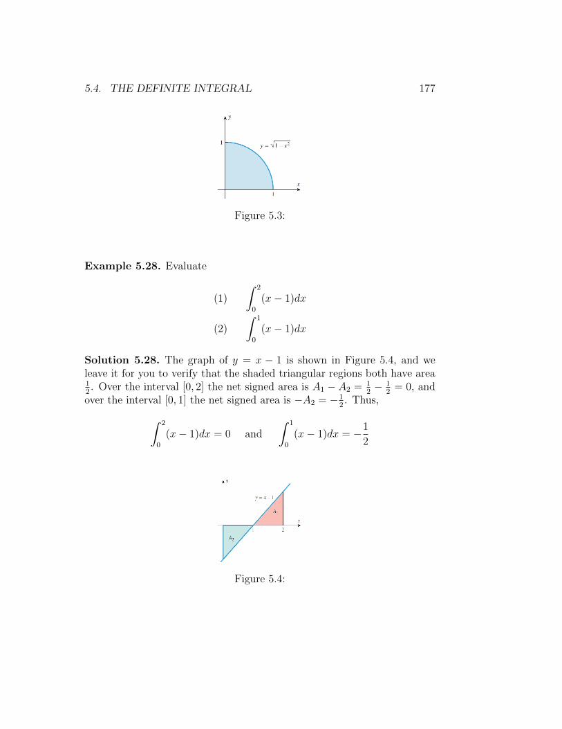
5.4. THE DEFINITE INTEGRAL 177
Figure 5.3:
Example 5.28. Evaluate
(1)
∫ 2
0
(x− 1)dx
(2)
∫ 1
0
(x− 1)dx
Solution 5.28. The graph of y = x − 1 is shown in Figure 5.4, and weleave it for you to verify that the shaded triangular regions both have area12. Over the interval [0, 2] the net signed area is A1 − A2 = 1
2− 1
2= 0, and
over the interval [0, 1] the net signed area is −A2 = −12. Thus,∫ 2
0
(x− 1)dx = 0 and
∫ 1
0
(x− 1)dx = −1
2
Figure 5.4:
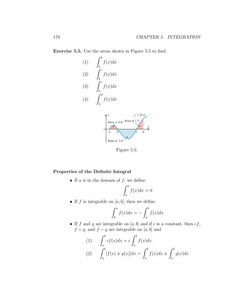
178 CHAPTER 5. INTEGRATION
Exercise 5.5. Use the areas shown in Figure 5.5 to find:
(1)
∫ b
a
f(x)dx
(2)
∫ c
b
f(x)dx
(3)
∫ c
a
f(x)dx
(4)
∫ d
a
f(x)dx
Figure 5.5:
Properties of the Definite Integral
• If a is in the domain of f , we define∫ a
a
f(x)dx = 0
• If f is integrable on [a, b], then we define∫ a
b
f(x)dx = −∫ b
a
f(x)dx
• If f and g are integrable on [a, b] and if c is a constant, then cf ,f + g, and f − g are integrable on [a, b] and
(1)
∫ b
a
cf(x)dx = c
∫ b
a
f(x)dx
(2)
∫ b
a
[f(x)± g(x)]dx =
∫ b
a
f(x)dx±∫ b
a
g(x)dx

5.4. THE DEFINITE INTEGRAL 179
• If f is integrable on a closed interval containing the three pointsa, b, and c, then∫ b
a
f(x)dx =
∫ c
a
f(x)dx+
∫ b
c
f(x)dx
no matter how the points are ordered.
• If f is integrable on [a, b] and f(x) ≥ 0 for all x in [a, b], then∫ b
a
f(x)dx ≥ 0
and if f(x) ≤ 0 for all x in [a, b], then∫ b
a
f(x)dx ≤ 0
• If f and g are integrable on [a, b] and f(x) ≥ g(x) for all x in[a, b], then ∫ b
a
f(x)dx ≥∫ b
a
g(x)dx
Example 5.29. Find ∫ 2
−1[f(x) + 2g(x)]dx
if ∫ 2
−1f(x)dx = 5 and
∫ 2
−1g(x)dx = −3
Solution 5.29.∫ 2
−1[f(x) + 2g(x)]dx =
∫ 2
−1f(x)dx+ 2
∫ 2
−1g(x)dx
= 5 + 2× (−3)
= −1
�
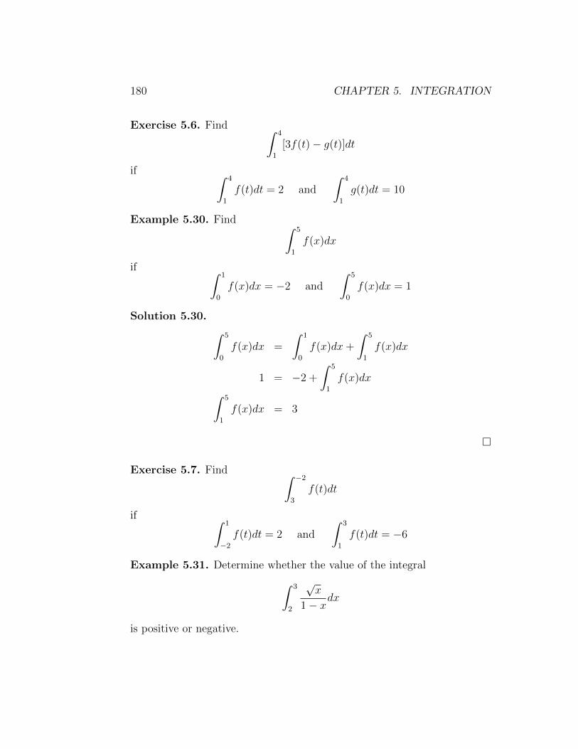
180 CHAPTER 5. INTEGRATION
Exercise 5.6. Find ∫ 4
1
[3f(t)− g(t)]dt
if ∫ 4
1
f(t)dt = 2 and
∫ 4
1
g(t)dt = 10
Example 5.30. Find ∫ 5
1
f(x)dx
if ∫ 1
0
f(x)dx = −2 and
∫ 5
0
f(x)dx = 1
Solution 5.30. ∫ 5
0
f(x)dx =
∫ 1
0
f(x)dx+
∫ 5
1
f(x)dx
1 = −2 +
∫ 5
1
f(x)dx∫ 5
1
f(x)dx = 3
�
Exercise 5.7. Find ∫ −23
f(t)dt
if ∫ 1
−2f(t)dt = 2 and
∫ 3
1
f(t)dt = −6
Example 5.31. Determine whether the value of the integral∫ 3
2
√x
1− xdx
is positive or negative.

5.5. THE FUNDAMENTAL THEOREM OF CALCULUS 181
Solution 5.31. Since√x > 0 and 1− x < 0 on [2, 3] then
√x
1− x< 0 and
∫ 3
2
√x
1− xdx < 0
�
Exercise 5.8. Determine whether the value of the integral∫ 4
0
t2
3− cos tdt
is positive or negative.
5.5 The Fundamental Theorem of Calculus
In this section we will establish two basic relationships between definiteand indefinite integrals that together constitute a result called the Funda-mental Theorem of Calculus. One part of this theorem will relate theantiderivative method for calculating areas, and the second part will providea powerful method for evaluating definite integrals using antiderivatives.
The first part of the Fundamental Theorem of Calculus says that: Thedefinite integral can be evaluated by finding any antiderivative of the in-tegrand and then subtracting the value of this antiderivative at the lowerlimit of integration from its value at the upper limit of integration.
Theorem 5.5.1. If f is continuous on [a, b] and F is any antiderivative off on [a, b], then ∫ b
a
f(x)dx = F (x)]ba = F (b)− F (a)
Observe that in the preceding theorem we did not include a constantof integration in the antiderivatives. In general, when applying the Fun-damental Theorem of Calculus there is no need to include a constant ofintegration because it will drop out anyway.

182 CHAPTER 5. INTEGRATION
Example 5.32. Evaluate
(1)
∫ 4
1
3dx
(2)
∫ 9
1
xdx
(3)
∫ π/3
0
sec2 xdx
(4)
∫ ln 3
0
5exdx
(5)
∫ −1−e
1
xdx
(6)
∫ 1/2
−1/2
1√1− x2
dx
Solution 5.32.
(1)
∫ 4
1
3dx = 3x]41 = 3(4)− 3(1) = 9
(2)
∫ 9
1
xdx =1
2x2]91
=1
2(9)2 − 1
2(1)2 = 40
(3)
∫ π/3
0
sec2 xdx = tanx]π/30 = tanπ
3− tan 0 =
√3− 0 =
√3
(4)
∫ ln 3
0
5exdx = 5ex]ln 30 = 5eln 3− 5e0 = 5(3)− 5(1) = 10
(5)
∫ −1−e
1
xdx = ln |x|]−1−e = ln | − 1| − ln | − e| = 0− 1 = −1
(6)
∫ 1/2
−1/2
1√1− x2
dx = sin−1 x]1/2−1/2 = sin−1
(1
2
)− sin−1
(−1
2
)=π
6− −π
6=π
3
�
Example 5.33. Evaluate∫ 3
0
f(x)dx if f(x) =
{x2 if x < 23x− 2 if x ≥ 2

5.5. THE FUNDAMENTAL THEOREM OF CALCULUS 183
Solution 5.33. From the properties of definite integral we can integratefrom 0 to 2 and from 2 to 3 separately and add the results. This yields∫ 3
0
f(x)dx =
∫ 2
0
f(x)dx+
∫ 3
2
f(x)dx =
∫ 2
0
x2dx+
∫ 3
2
(3x− 2)dx
=x3
3
]20
+
(3x2
2− 2x
)]32
=
(8
3− 0
)+
(15
2− 2
)=
49
6
�
Exercise 5.9. Evaluate the integrals using Part 1 of the Fundamental The-orem of Calculus.
(1)
∫ 2
−14t(1− t2
)dt
(2)
∫ π/2
−π/2sin tdt
(3)
∫ 1
−1|2t− 1|dt
The next theorem describes the method for evaluating definite integralsin which a substitution is required.
Theorem 5.5.2. If g′ is continuous on [a, b] and f is continuous on aninterval containing the values of g(x) for a ≤ x ≤ b, then∫ b
a
f(g(x))g′(x)dx =
∫ g(b)
g(a)
f(u)du
Example 5.34. Evaluate ∫ 2
0
x(x2 + 1
)3dx
Solution 5.34. If we let u = x2 + 1 so that du = 2xdx or 12du = xdx, then
if x = 0 , u = 1
if x = 2 , u = 5

184 CHAPTER 5. INTEGRATION
Thus, ∫ 2
0
x(x2 + 1
)3dx =
1
2
∫ 5
1
u3du
=u4
8
]51
=625
8− 1
8= 78
�
Example 5.35. Evaluate ∫ π/8
0
sin5 2x cos 2xdx
Solution 5.35. If we let u = sin 2x so that du = 2 cos 2xdx or 12du =
cos 2xdx, then
if x = 0 , u = sin(0) = 0
if x =π
8, u = sin(π/8) =
1√2
Thus, ∫ π/8
0
sin5 2x cos 2xdx =1
2
∫ 1/√2
0
u5du
=u6
12
]1/√20
=1
12(√
2)6 − 0 =
1
96
�
Exercise 5.10. Evaluate the integrals.
(1)
∫ π/4
0
tan2 t sec2 tdt
(2)
∫ 1
0
t3√t2 + 3dt
(3)
∫ √e1
1
t√
1− (ln t)2dt
5.5. THE FUNDAMENTAL THEOREM OF CALCULUS 185
Example 5.36. Find∫ 0
−2xf(x2)dx if
∫ 4
0
f(x)dx = 1
Solution 5.36. If we let u = x2 so that du = 2xdx or 12du = xdx, then
if x = −2 , u = 4
if x = 0 , u = 0
Thus, ∫ 0
−2xf(x2)dx =
1
2
∫ 4
0
f(u)du =1
2× 1 =
1
2
�
Exercise 5.11. Find∫ 1
0
f(3t+ 1)dt if
∫ 4
1
f(t)dt = 5
The second part of the Fundamental Theorem of Calculus says: If adefinite integral has a variable upper limit of integration, a constant lowerlimit of integration, and a continuous integrand, then the derivative of theintegral with respect to its upper limit is equal to the integrand evaluatedat the upper limit.
Theorem 5.5.3. If f is continuous on an interval, then f has an an-tiderivative on that interval. In particular, if a is any point in the interval,then the function F defined by
F (x) =
∫ x
a
f(t)dt
is an antiderivative of f ; that is, F ′(x) = f(x) for each x in the interval,or in an alternative notation
d
dx
[∫ x
a
f(t)dt
]= f(x)
186 CHAPTER 5. INTEGRATION
Corollary 5.5.4.
(1)d
dx
[∫ h(x)
a
f(t)dt
]= f(h(x)) · h′(x)
(2)d
dx
[∫ h(x)
l(x)
f(t)dt
]= f(h(x)) · h′(x)− f(l(x)) · l′(x)
Example 5.37. Findd
dx
[∫ x
1
t3dt
]Solution 5.37. The integrand is a continuous function, so
d
dx
[∫ x
1
t3dt
]= x3
�
Example 5.38. Findd
dx
[∫ x
1
sin t
tdt
]Solution 5.38. The integrand is a continuous on any interval that doesnot contain the origin, so on the interval (0,∞) we have
d
dx
[∫ x
1
sin t
tdt
]=
sinx
x
�
Example 5.39. Use the part 2 of the Fundamental Theorem of Calculusto find
d
dx
[∫ x2
1
etdt
]Solution 5.39. The integrand is a continuous function, so
d
dx
[∫ x2
1
etdt
]= ex
2 d
dx
(x2)
= 2xex2
5.5. THE FUNDAMENTAL THEOREM OF CALCULUS 187
Example 5.40. Use the part 2 of the Fundamental Theorem of Calculusto find
d
dx
[∫ cosx
sinx
t2dt
]Solution 5.40. The integrand is a continuous function, so
d
dx
[∫ cosx
sinx
t2dt
]= cos2 x
d
dx(cosx)− sin2 x
d
dx(sinx)
= − sinx cos2 x− cosx sin2 x
�
Exercise 5.12. Use the part 2 of the Fundamental Theorem of Calculusto find
(1)d
dx
[x
∫ x2
2
sin(t3)dt
]
(2)d
dx
[∫ 1
2x
3√tdt
](3)
d
dx
[∫ x2
−xsin−1 tdt
]The two parts of the Fundamental Theorem of Calculus, when taken
together, tell us that differentiation and integration are inverse processes inthe sense that each undoes the effect of the other. To see why this is so,note that Part 1 of the Fundamental Theorem of Calculus implies that∫ x
a
f ′(t)dt = f(x)− f(a)
which tells us that if the value of f(a) is known, then the function f canbe recovered from its derivative f ′ by integrating. Conversely, Part 2 of theFundamental Theorem of Calculus states that
d
dx
[∫ x
a
f(t)dt
]= f(x)
which tells us that the function f can be recovered from its integral by dif-ferentiating. Thus, differentiation and integration can be viewed as inverseprocesses.

188 CHAPTER 5. INTEGRATION
Example 5.41. Find a function f and a number a such that
6 +
∫ x
a
f(t)
t2dt = 2
√x for x ≥ 0
Solution 5.41. If we let x = a ≥ 0, we have
6 +
∫ a
a
f(t)
t2dt = 2
√a
6 + 0 = 2√a
a = 9
To find f , differentiate both sides of the equation with respect to x:
d
dx
[6 +
∫ x
a
f(t)
t2dt
]=
d
dx
[2√x]
0 +f(x)
x2=
1√x
f(x) =x2√x
=√x3 where x ≥ 0
�
Exercise 5.13. If
f(x) =
∫ x
0
(1− t2
)dt,
on what intervals is f increasing, decreasing, concave up or down, and whatare the extremum and inflection points, if any, of the function f?
5.6 Area Between Two Curves
In this section we review and extend the use of definite integrals to representplane areas. Recall that the integral∫ b
a
f(x)dx
measures the area between the graph of f and the x−axis from x = ato x = b, but treats as negative any part of this area that lies below the

5.6. AREA BETWEEN TWO CURVES 189
x−axis. (We are assuming that a < b.) In order to express the total areabounded by y = f(x), y = 0, x = a, and x = b, counting all of the areapositively, we should integrate the absolute value of f (see Figure 5.6):∫ b
a
f(x)dx = A1 − A2 and
∫ b
a
|f(x)|dx = A1 + A2
There is no rule for integrating∫ b
a
|f(x)|dx,
one must break the integral into a sum of integrals over intervals wheref(x) > 0 so |f(x)| = f(x), and intervals where f(x) < 0 so |f(x)| = −f(x).
Figure 5.6:
To find the area between the graph of f and the x−axis over the interval[a, b]:
1. Subdivide [a, b] at the zeros of f .
2. Integrate f over each subinterval.
3. Add the absolute values of the integrals.
Example 5.42. Figure 5.7 shows the graph of the function f(x) = sinxbetween x = 0 and x = 2π. Compute the area between the graph of f(x)and the x−axis over [0, 2π].

190 CHAPTER 5. INTEGRATION
Figure 5.7:
Solution 5.42. First find the zeros of f . On [0, 2π], the zeros of f(x) =sinx are x = 0, π , 2π. So, the area between the graph of f(x) and thex−axis over [0, 2π] is calculated by breaking up the domain of sinx intotwo pieces: the interval [0, π] over which it is nonnegative and the interval[π, 2π] over which it is nonpositive.∫ π
0
sinxdx = − cosx]π0 = −(cos π − cos 0) = 2∫ 2π
π
sinxdx = − cosx]2ππ = −(cos 2π − cos π) = −2
The second integral gives a negative value. The area between the graphand the axis is obtained by adding the absolute values
Area = |2|+ | − 2| = 4.
�
Example 5.43. Find the area of the region between the x−axis and thegraph of f(x) = x3 − x2 − 2x over [−1, 2].
Solution 5.43. First find the zeros of f . Since
f(x) = x3 − x2 − 2x = x(x2 − x− 2) = x(x+ 1)(x− 2),
the zeros are x = 0, −1 and 2 (Figure 5.8). The zeros subdivide [−1, 2]into two subintervals: [−1, 0] on which f ≥ 0 and [0, 2], on which f ≤ 0.
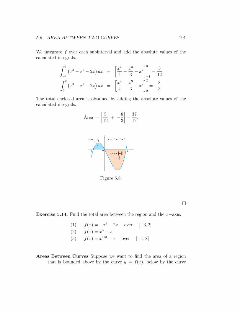
5.6. AREA BETWEEN TWO CURVES 191
We integrate f over each subinterval and add the absolute values of thecalculated integrals.∫ 0
−1
(x3 − x2 − 2x
)dx =
[x4
4− x3
3− x2
]0−1
=5
12∫ 2
0
(x3 − x2 − 2x
)dx =
[x4
4− x3
3− x2
]20
= −8
3
The total enclosed area is obtained by adding the absolute values of thecalculated integrals.
Area =
∣∣∣∣ 5
12
∣∣∣∣+
∣∣∣∣−8
3
∣∣∣∣ =37
12.
Figure 5.8:
�
Exercise 5.14. Find the total area between the region and the x−axis.
(1) f(x) = −x2 − 2x over [−3, 2]
(2) f(x) = x3 − x(3) f(x) = x1/3 − x over [−1, 8]
Areas Between Curves Suppose we want to find the area of a regionthat is bounded above by the curve y = f(x), below by the curve

192 CHAPTER 5. INTEGRATION
Figure 5.9:
y = g(x) and on the left and right by the lines x = a and x = b(Figure 5.9). The region might accidentally have a shape whose areawe could find with geometry, but if f and g are arbitrary continuousfunctions, we usually have to find the area with an integral.
Definition 5.6.1. If f and g are continuous throughout [a, b], thenthe area of the region between the curves f(x) and g(x) from a to bis the integral of |f − g| from a to b:
A =
∫ b
a
|f(x)− g(x)|dx.
When applying this definition it is helpful to graph the curves. Ithelps you find the limits of integration if they are not given. Youmay need to find where the curves intersect to determine the limits ofintegration, and this may involve solving the equation f(x) = g(x) forvalues of x. Then you can integrate the function for the area betweenthe intersections.
Example 5.44. Find the area of the region bounded above by thecurve y = 2e−x + x, below by the curve y = 1
2ex, on the left by x = 0,
and on the right by x = 1.
Solution 5.44. Figure 5.10 displays the graphs of the curves and theregion whose area we want to find. The area between the curves over

5.6. AREA BETWEEN TWO CURVES 193
the interval is given by∫ 1
0
∣∣∣∣(2e−x + x)− 1
2ex∣∣∣∣ =
∣∣∣∣∣[−2e−x +
x2
2− 1
2ex]10
∣∣∣∣∣= 3− 2
e− e
2≈ 0.9051
Figure 5.10:
Example 5.45. Find the area of the region enclosed by the parabolay = 2− x2 and the line y = −x.
Solution 5.45. First we sketch the two curves (Figure 5.11). Thelimits of integration are found by solving y = 2 − x2 and y = −xsimultaneously for x.
2− x2 = −xx2 − x− 2 = 0
(x+ 1)(x− 2) = 0
x = −1 or x = 2
The region runs from x = −1 to x = 2. The limits of integration area = −1 and b = 2. The area between the curves is∫ 2
−1
∣∣(2− x2)− (−x)∣∣ =
∫ 2
−1
∣∣2 + x− x2∣∣
=
∣∣∣∣∣[2x+
x2
2− x3
3
]2−1
∣∣∣∣∣ =9
2
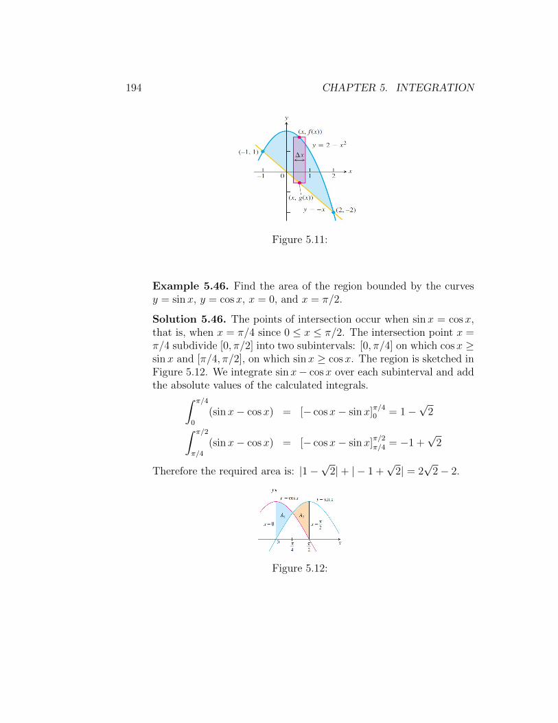
194 CHAPTER 5. INTEGRATION
Figure 5.11:
Example 5.46. Find the area of the region bounded by the curvesy = sinx, y = cosx, x = 0, and x = π/2.
Solution 5.46. The points of intersection occur when sinx = cosx,that is, when x = π/4 since 0 ≤ x ≤ π/2. The intersection point x =π/4 subdivide [0, π/2] into two subintervals: [0, π/4] on which cosx ≥sinx and [π/4, π/2], on which sinx ≥ cosx. The region is sketched inFigure 5.12. We integrate sin x− cosx over each subinterval and addthe absolute values of the calculated integrals.∫ π/4
0
(sinx− cosx) = [− cosx− sinx]π/40 = 1−√
2∫ π/2
π/4
(sinx− cosx) = [− cosx− sinx]π/2π/4 = −1 +
√2
Therefore the required area is: |1−√
2|+ | − 1 +√
2| = 2√
2− 2.
Figure 5.12:

Appendix A
Solving Equations andInequalities
The Cartesian Plane: Just as you can represent real numbers by pointson a real number line, you can represent ordered pairs of real numbersby points in a plane called the rectangular coordinate system, or theCartesian plane.The Cartesian plane is formed by using two real number lines inter-secting at right angles, as shown in Figure A.1. The horizontal realnumber line is usually called the x−axis, and the vertical real numberline is usually called the y−axis. The point of intersection of these twoaxes is the origin, and the two axes divide the plane into four partscalled quadrants. Each point in the plane corresponds to an ordered
Figure A.1:
pair (x, y) of real numbers x and y, called coordinates of the point.
195

196 APPENDIX A. SOLVING EQUATIONS AND INEQUALITIES
The x−coordinate represents the directed distance from the y−axisto the point, and the y−coordinate represents the directed distancefrom the x-axis to the point, as shown in Figure A.2.
Figure A.2:
Example A.1. Plot the points (−1, 2), (3, 4), (0, 0), (3, 0), and (−2,−3).
Solution A.1. See Figure A.3 below.
Figure A.3:
�
Suppose you want to determine the distance d between two points(x1, y1) and (x2, y2) in the plane, use the distance formula.
Theorem A.0.1. The distance d between two points (x1, y1) and(x2, y2) in the plane is
d =√
(x2 − x1)2 + (y2 − y1)2
197
Example A.2. Find the distance between the points (−2, 1) and(3, 4).
Solution A.2. Let (x1, y1) = (−2, 1) and (x2, y2) = (3, 4). Then
d =√
(x2 − x1)2 + (y2 − y1)2
=√
(3− (−2))2 + (4− 1)2
=√
52 + 32
=√
34
�
To find the midpoint of the line segment that joins two points (x1, y1)and (x2, y2) in a coordinate plane, find the average values of the respec-tive coordinates of the two endpoints using the Midpoint Formula.
Midpoint =
(x1 + x2
2,y1 + y2
2
)Example A.3. Find the midpoint of the line segment joining thepoints (−5,−3) and (9, 3).
Solution A.3. Let (x1, y1) = (−5,−3) and (x2, y2) = (9, 3). Then
Midpoint =
(x1 + x2
2,y1 + y2
2
)=
(−5 + 9
2,−3 + 3
2
)= (2, 0)
�
Solving Equations Algebraically An equation in x is a statement thattwo algebraic expressions are equal. For example, 3x−5 = 7, x2−x−6 = 0, and
√2x = 4 are equations. To solve an equation in x means
to find all values of x for which the equation is true. Such values aresolutions. For instance, x = 4 is a solution of the equation 3x− 5 = 7because 3(4)−5 = 7 is a true statement. The solutions of an equation
198 APPENDIX A. SOLVING EQUATIONS AND INEQUALITIES
depend on the kinds of numbers being considered. For instance, inthe set of rational numbers, x2 = 10 has no solution because there isno rational number whose square is 10. However, in the set of realnumbers, the equation has the two solutions
√10 and −
√10.
An equation that is true for every real number in the domain (thedomain is the set of all real numbers for which the equation is defined)of the variable is called an identity. For example, x2−9 = (x+3)(x−3)is an identity because it is a true statement for any real value of x,and x/(3x2) = 1/(3x), where x 6= 0, is an identity because it is truefor any nonzero real value of x. An equation that is true for just some(or even none) of the real numbers in the domain of the variable iscalled a conditional equation. The equation x2 − 9 = 0 is conditionalbecause x = 3 and x = −3 are the only va1ues in the domain thatsatisfy the equation. The equation 2x+ 1 = 2x− 3 is also conditionalbecause there are no real values of x for which the equation is true.
Polynomial equations can be classified by their degree. The degree ofa polynomial equation is the highest degree of its terms. In general,the higher the degree, the more difficult it is to solve the equationeither algebraically or graphically. You should be familiar with thefollowing four methods for solving quadratic equations algebraically:
• Factoring: if a× b = 0 then a = 0 or b = 0. The following aresome important factorizations.
* a2 − b2 = (a− b)(a+ b).
* a3 − b3 = (a− b)(a2 + ab+ b2).
* a3 + b3 = (a+ b)(a2 − ab+ b2).
* a4 − b4 = (a− b)(a+ b)(a2 + b2).
• Extracting Square Roots: if x2 = c, where c > 0, then x =±√c.
• Completing the Square: if x2+bx = c, then(x+ b
2
)2= c+ b2
4.
• Quadratic Formula: if ax2 + bx+ c = 0 then x = −b±√b2−4ac2a
.
Example A.4. Solve x2 − 5x+ 4 = 0.

199
Solution A.4.
x2 − 5x+ 4 = 0
(x− 1)(x− 4) = 0
(x− 1) = 0 ↪→ x = 1
or (x− 4) = 0 ↪→ x = 4
�
Example A.5. Solve (x+ 3)2 = 16.
Solution A.5.
(x+ 3)2 = 16
(x+ 3) = ±4
x = −3± 4⇒ x = 1 or x = −7
�
Example A.6. Solve x2 + 6x = 5.
Solution A.6.
x2 + 6x = 5(x+
6
2
)2
= 5 +62
4
(x+ 3)2 = 14
x+ 3 = ±√
14
x = −3±√
14
�
Example A.7. Solve 2x2 + 3x− 1 = 0.
Solution A.7.
2x2 + 3x− 1 = 0
x =−3±
√32 − 4(2)(−2)
2(2)
x =−3±
√17
4
200 APPENDIX A. SOLVING EQUATIONS AND INEQUALITIES
The methods used to solve quadratic equations can sometimes beextended to polynomial equations of higher degree, as shown in thenext two examples.
Example A.8. Solve x4 − 3x2 + 2 = 0
Solution A.8. The expression x4− 3x2 + 2 is said to be in quadraticform because it is written in the form au2 + bu + c, where u is anyexpression in x, namely x2. You can use factoring to solve the equationas follows.
x4 − 3x2 + 2 = 0
(x2)2 − 3(x2) + 2 = 0
(x2 − 1)(x2 − 2) = 0
(x− 1)(x+ 1)(x2 − 2) = 0
x− 1 = 0 ⇒ x = 1
or x+ 1 = 0 ⇒ x = −1
or x2 − 2 = 0 ⇒ x = ±√
2
�
Example A.9. Solve 2x3 − 6x2 − 6x+ 18 = 0.
Solution A.9. This equation has a common factor of 2. You cansimplify the equation by first dividing each side of the equation by 2.
2x3 − 6x2 − 6x+ 18 = 0
x3 − 3x2 − 3x+ 9 = 0
x2(x− 3)− 3(x− 3) = 0
(x− 3)(x2 − 3) = 0
x− 3 = 0 ⇒ x = 3
or x2 − 3 = 0 ⇒ x = ±√
3
�
An equation involving a radical expression can often be cleared ofradicals by raising each side of the equation to an appropriate power.

201
When using this procedure, it is crucial to check for extraneous solu-tions because of the restricted domain of a radical equation.
Example A.10. Solve√
2x+ 7− x = 2
Solution A.10.√
2x+ 7− x = 2√2x+ 7 = x+ 2
2x+ 7 = x2 + 4x+ 4
x2 + 2x− 3 = 0
(x+ 3)(x− 1) = 0
x+ 3 = 0 ⇒ x = −3
x− 1 = 0 ⇒ x = 1
By substituting into the original equation, you can determine thatx = −3 is extraneous, whereas x = 1 is valid. So, the equation hasonly one real solution: x = 1.
�
Example A.11. Solve√
2x+ 6−√x+ 4 = 1
Solution A.11.√
2x+ 6−√x+ 4 = 1√
2x+ 6 = 1 +√x+ 4
2x+ 6 = 1 + 2√x+ 4 + (x+ 4)
x+ 1 = 2√x+ 4
x2 + 2x+ 1 = 4(x+ 4)
x2 − 2x− 15 = 0
(x− 5)(x+ 3) = 0
x− 5 = 0 ⇒ x = 5
x+ 3 = 0 ⇒ x = −3
By substituting into the original equation, you can determine thatx = −3 is extraneous, whereas x = 5 is valid. So that x = 5 is theonly solution.

202 APPENDIX A. SOLVING EQUATIONS AND INEQUALITIES
Example A.12. Solve (x+ 1)2/3 = 4
Solution A.12.
(x+ 1)2/3 = 43√
(x+ 1)2 = 4
(x+ 1)2 = 64
x+ 1 = ±8
x = 7 or − 9
�
Example A.13. Solve 2x
= 3x−2 − 1
Solution A.13. For this equation, the least common denominator ofthe three terms is x(x−2), so you can begin by multiplying each termof the equation by this expression.
2
x=
3
x− 2− 1
x(x− 2)2
x= x(x− 2)
3
x− 2− x(x− 2)
2(x− 2) = 3x− x(x− 2); x 6= 0, 2
x2 − 3x− 4 = 0
(x− 4)(x+ 1) = 0
x− 4 = 0 ⇒ x = 4
x+ 1 = 0 ⇒ x = −1
�
Solving Inequalities Algebraically The inequality symbols<,≤, >, and≥ are used to compare two numbers and to denote subsets of realnumbers. For instance, the simple inequality x ≥ 3 denotes all realnumbers x that are greater than or equal to 3.
As with an equation, you solve an inequality in the variable x byfinding all values of x for which the inequality is true. These values aresolutions of the inequality and are said to satisfy the inequality. For

203
instance, the number 9 is a solution of the inequality 5x− 7 > 3x+ 9because
5(9)− 7 > 3(9) + 9
38 > 36
On the other hand, the number 7 is not a solution because
5(7)− 7 ≯ 3(7) + 9
28 ≯ 30
The set of all real numbers that are solutions of an inequality is thesolution set of the inequality. The procedures for solving linear in-equalities in one variable are much like those for solving linear equa-tions. To isolate the variable, you can make use of the properties ofinequalities, see Theorem A.0.2. These properties are similar to theproperties of equality, but there are two important exceptions. Wheneach side of an inequality is multiplied or divided by a negative num-ber, the direction of the inequality symbol must be reversed in orderto maintain a true statement.
Theorem A.0.2. Let a, b, c and d be real numbers.
1. Transitive Property: if a < b and b < c, then a < c
2. Addition of Inequalities: if a < b and c < d, then a+ c < b+ d
3. Addition of a Constant: if a < b, then a+ c < b+ c
4. Multiplying by a Constant: we have two cases
a) for c > 0, if a < b, then ac < bc
b) for c < 0, if a < b, then ac > bc
Each of the properties above is true if the symbol < is replaced by ≤and > is replaced by ≥.
Example A.14. Solve 2x+ 1 ≤ 5x− 8.
Solution A.14.
2x+ 1 ≤ 5x− 8
−3x ≤ −9
x ≥ 3

204 APPENDIX A. SOLVING EQUATIONS AND INEQUALITIES
So, the solution set is all real numbers that are greater than or equalto 3. The interval notation for this solution set is [3,∞).
�
Example A.15. Solve 1− 32x ≥ x− 4.
Solution A.15.
1− 3
2x ≥ x− 4
2− 3x ≥ 2x− 8
−5x ≥ −10
x ≤ 2
So, the solution set is all real numbers that are less than or equal to2. The interval notation for this solution set is (−∞, 2].
�
Sometimes it is possible to write two inequalities as a double inequal-ity, as demonstrated in the following example.
Example A.16. Solve 1 < 1− 3x ≤ 6.
Solution A.16.
1 < 1− 3x ≤ 6
0 < −3x ≤ 5
0 > x ≥ −5
3
−5
3≤ x < 0
The solution set is all real numbers that are greater than or equalto −5
3and less than 0. The interval notation for this solution set is[
−53, 0).
�
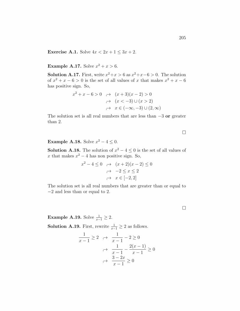
205
Exercise A.1. Solve 4x < 2x+ 1 ≤ 3x+ 2.
Example A.17. Solve x2 + x > 6.
Solution A.17. First, write x2+x > 6 as x2+x−6 > 0. The solutionof x2 + x − 6 > 0 is the set of all values of x that makes x2 + x − 6has positive sign. So,
x2 + x− 6 > 0 ↪→ (x+ 3)(x− 2) > 0
↪→ (x < −3) ∪ (x > 2)
↪→ x ∈ (−∞,−3) ∪ (2,∞)
The solution set is all real numbers that are less than −3 or greaterthan 2.
�
Example A.18. Solve x2 − 4 ≤ 0.
Solution A.18. The solution of x2 − 4 ≤ 0 is the set of all values ofx that makes x2 − 4 has non positive sign. So,
x2 − 4 ≤ 0 ↪→ (x+ 2)(x− 2) ≤ 0
↪→ −2 ≤ x ≤ 2
↪→ x ∈ [−2, 2]
The solution set is all real numbers that are greater than or equal to−2 and less than or equal to 2.
�
Example A.19. Solve 1x−1 ≥ 2.
Solution A.19. First, rewrite 1x−1 ≥ 2 as follows.
1
x− 1≥ 2 ↪→ 1
x− 1− 2 ≥ 0
↪→ 1
x− 1− 2(x− 1)
x− 1≥ 0
↪→ 3− 2x
x− 1≥ 0
206 APPENDIX A. SOLVING EQUATIONS AND INEQUALITIES
The solution of 3−2xx−1 ≥ 0; x 6= 1 is the set of all values of x that makes
3−2xx−1 has non negative sign. So,
3− 2x
x− 1≥ 0 ↪→ 1 < x ≤ 3
2
↪→ x ∈(
1,3
2
]
�
Exercise A.2. Solve the following inequalities.
(a) 1x2+1
> 0
(b) x2 + 4 < 0
(c) −3 < 1x≤ 1
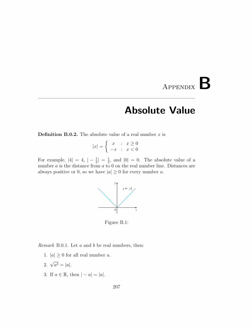
Appendix B
Absolute Value
Definition B.0.2. The absolute value of a real number x is
|x| ={
x : x ≥ 0−x : x < 0
For example, |4| = 4, | − 12| = 1
2, and |0| = 0. The absolute value of a
number a is the distance from a to 0 on the real number line. Distances arealways positive or 0, so we have |a| ≥ 0 for every number a.
Figure B.1:
Remark B.0.1. Let a and b be real numbers, then:
1. |a| ≥ 0 for all real number a.
2.√a2 = |a|.
3. If a ∈ R, then | − a| = |a|.
207
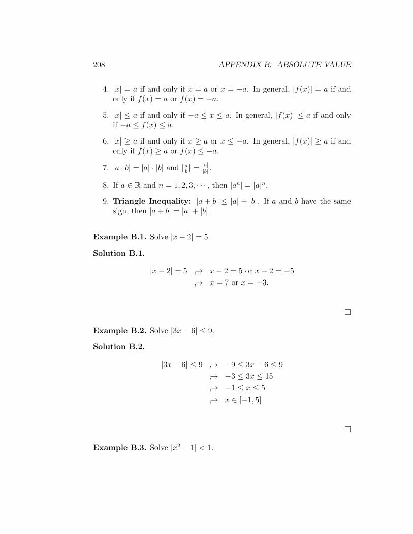
208 APPENDIX B. ABSOLUTE VALUE
4. |x| = a if and only if x = a or x = −a. In general, |f(x)| = a if andonly if f(x) = a or f(x) = −a.
5. |x| ≤ a if and only if −a ≤ x ≤ a. In general, |f(x)| ≤ a if and onlyif −a ≤ f(x) ≤ a.
6. |x| ≥ a if and only if x ≥ a or x ≤ −a. In general, |f(x)| ≥ a if andonly if f(x) ≥ a or f(x) ≤ −a.
7. |a · b| = |a| · |b| and |ab| = |a|
|b| .
8. If a ∈ R and n = 1, 2, 3, · · · , then |an| = |a|n.
9. Triangle Inequality: |a + b| ≤ |a| + |b|. If a and b have the samesign, then |a+ b| = |a|+ |b|.
Example B.1. Solve |x− 2| = 5.
Solution B.1.
|x− 2| = 5 ↪→ x− 2 = 5 or x− 2 = −5
↪→ x = 7 or x = −3.
�
Example B.2. Solve |3x− 6| ≤ 9.
Solution B.2.
|3x− 6| ≤ 9 ↪→ −9 ≤ 3x− 6 ≤ 9
↪→ −3 ≤ 3x ≤ 15
↪→ −1 ≤ x ≤ 5
↪→ x ∈ [−1, 5]
�
Example B.3. Solve |x2 − 1| < 1.
209
Solution B.3.
|x2 − 1| < 1 ↪→ −1 < x2 − 1 < 1
↪→ 0 < x2 < 2
↪→ 0 <√x2 <
√2
↪→ 0 < |x| <√
2
↪→ (|x| > 0) ∩ (|x| <√
2)
↪→ (R− {0}) ∩ (−√
2 < x <√
2)
↪→ x ∈ (R− {0}) ∩ (−√
2,√
2)
↪→ x ∈ (−√
2,√
2)− {0}
�
Example B.4. Solve |x+ 4| > 7.
Solution B.4.
|x+ 4| > 7 ↪→ x+ 4 > 7 or x+ 4 < −7
↪→ x > 3 or x < −11
↪→ x ∈ (−∞,−11) ∪ (3,∞)
�
Exercise B.1. Solve the following equations and inequalities.
(a) 1 ≤ |x| ≤ 4
(b) |x+ 3| = |1 + 2x|
(c) |x2 − 9| = 9− x2


Appendix C
Equation of Line
Definition C.0.3. For x1 6= x2, the slope of the straight line through thepoints (x1, y1) and (x2, y2) is the number m = y2−y1
x2−x1 .
Figure C.1:
Example C.1. Find the slope of the line through the points (−3, 5) and(2,−4).
Solution C.1. The slope is m = −4−52−(−3) = −9
5.
�
211
212 APPENDIX C. EQUATION OF LINE
Remark C.0.2. (Vertical and Horizontal Lines)
• When x1 = x2, the line is vertical and the slope is undefined. Theequation of the line in this case is x = x1.
• When y1 = y2, the line is horizontal and the slope is zero. The equa-tion of the line in this case is y = y1.
Remark C.0.3. The point-slope form of a line is y− y0 = m (x− x0), wherethe line passes through (x0, y0) with slope m.
Example C.2. Find the equation of the line that passes through the point(2, 1) with slope 2
3.
Solution C.2.
y − y0 = m(x− x0)
y − 1 =2
3(x− 2)
y − 1 =2
3x− 4
3
y =2
3x− 1
3
�
Example C.3. Find an equation of the line through the points (3, 1) and(4,−1).
Solution C.3. The slope is m = −1−14−3 = −2. So, the equation is
y − y0 = m(x− x0)y − 1 = −2(x− 3)
y − 1 = −2x+ 6
y = −2x+ 7
�
213
Remark C.0.4. The equation y = mx+ b is called the slope-intercept form,where m is the slope and b is the y−intercept. The x−intercept is x = − b
m.
Figure C.2:
Example C.4. If a line has an equation y + 2x − 7 = 0, find the x− andy−intercepts of the line.
Solution C.4. 1. To find the x−intercept, let y = 0 in the equation ofthe line.
0 + 2x− 7 = 0 ↪→ x =7
2.
2. To find the y−intercept, let x = 0 in the equation of the line.
y + 0− 7 = 0 ↪→ y = 7.
�
Example C.5. Find the slope and y−intercept of the line y = −2.
Solution C.5. The slope is m = 0 (see remark C.0.2), and the y−interceptis −2.
�
Example C.6. If the point (2, k) lies on the line with slope 3 and passingthrough the point (1, 6), find the value of k.
214 APPENDIX C. EQUATION OF LINE
Solution C.6.
The slope of the line is m =k − 6
2− 13 = k − 6
9 = k
�
Theorem C.0.3. (Parallel and Perpendicular Lines) Two lines of slopem1 and m2 are parallel if m1 = m2, and are perpendicular if m1 ·m2 = −1.
Example C.7. Find an equation for the line parallel to y = 3x − 2 andpasses through the point (−1, 3).
Solution C.7. The slope of our line is the same as of y = 3x−2 since theyare parallel. Hence the slope is m = 3. The equation of line is
y − y0 = m(x− x0)y − 3 = 3(x− (−1))
y − 3 = 3x+ 3
y = 3x+ 6
�
Example C.8. Find an equation for the line perpendicular to y = −2x+4at the point (1, 2).
Solution C.8. The slope of our line equals −1/( slope of y = −2x + 4)since they are perpendicular. Hence the slope is m = −1
−2 = 0.5. Theequation of line is
y − y0 = m(x− x0)y − 2 = 0.5(x− 1)
y − 2 = 0.5x− 0.5
y = 0.5x+ 1.5
215
Example C.9. For what values of k will be the line kx + 5y = 2k beperpendicular to the line 2x+ 3y = 1.
Solution C.9. First, write the equations of lines in standard form as fol-lows.
kx+ 5y = 2k ↪→ y = −1
5kx+
2
5k (its slope is m1 = −1
5k)
2x+ 3y = 1 ↪→ y = −2
3x+
1
3(its slope is m2 = −2
3)
The lines are perpendicular if
m1 ×m2 = −1 ↪→ −1
5k ×−2
3= −1
↪→ k = −15
2
�
Exercise C.1. Find an equation for the line passes through the point (2, 7)and perpendicular to the x−axis.


Appendix D
Final Answers of Exercises
Chapter One
1. (a) R− {1} (b) R2. (a) [0,∞) (b) (∞, 0] (c) (0, 1]
3. (a) x = 3π/2 ± 2nπ (b) x = ±nπ (c) x = π/4 ± nπ (d)x = ±π/3± 2nπ (e) π/4± nπ/2
4. (a) R (b) [0 ± 2nπ, π/2 ± 2nπ)⋃
[π ± 2nπ, 3π/2 ± 2nπ) (c)x = ±nπ
5. (f−g)(x) = 2−1/x and its domain is R−{0}. Also, (f−g)(2) =3/2
6. f−1(x) = x/(1− x)
7. [−√
5,−√
3]⋃
[√
3,√
5]
8. (1) π/16 (2) −π/2 (3) 2π/3 (4) 5/12 (5) 4/√
7 (6) 1/√
5 (7)24/25
9. 5
10. (1) x = ±e2 (2) x = 2 (3) x = 4 (4) x =√
3/2 (5) x = ln 3(6) x = ee
11. (1) R (2) [0 ± 2nπ, π/2 ± 2nπ)⋃
(3π/2 ± 2nπ, 2π ± 2nπ] (3)(−∞, 0) (4) R− {0} (5) (1/e,∞) (6) (−∞, 1) (7) (−∞, 4)
12. (1) g−1(t) = (1 + log3 t)/2 (2) g−1(t) = 10t − 3
13. (1) 1 (2) 3/4 (3) 1
217

218 APPENDIX D. FINAL ANSWERS OF EXERCISES
14. sinh x = 12, coshx = 13. Now the other values are easy!!
15. sinh x = 4/3 only since x > 0. Now the other values are easy!!
Chapter Two
1. (1) 3 (2) 4 (3) 2 (4) does not exist (5) 2
2. (1) −1/12 (2) 0
3. (1) 1/128 (2) 12
4. 2
5. −1/2
6. 2, −2, the limit does not exist.
7. Does not exist.
8. 7
9. Both limits are 0
10. Does not exist.
11. (1) −1 (2) ∞ (3) 0
12. (1) Vertical: x = 3, Horizontal: y = 1 (2) Vertical: x = 0,Oblique: y = x
13. Easy!!
14. 4/5
15. −π and the second limit does not exist.
16. g continuous on R− {−2, 2, 4, 6, 8}17. 1 = limx→0 f(x) 6= f(0) = 0
18. (0,∞)− {1}19. (a) a = 10 (b) a = b = 1/2
20. 0
Chapter Three
1. −1/25
2. f ′(x) = 1/2√x, so f ′(0) does not exist.
3. df/dx = 2 at x = −1, and df−1/dx = 1/2 at x = f(−1) = 1
219
4. (1) (1 + 3x)/(2√x) (2) 2x ln 2− 2x (3) ex/(1 + x2) + ex tan−1 x
(4) 2x(7x+ 10)/(7x+ 5)2 (5) x coshx
5. m = 4, b = −4
6. (1) f = x9, c = 1, limit= 9 (2) f = 4√x, c = 16, limit= 1/32
7. f ′′ = 2/x3, f ′′′(2) = −3/8
8. − cosx
9. (1) n! (2) (−1)n 1xn+1
10. (1) 3 (4x3 − 6x) (x4 − 3x2 + 5)2(2) sec−1 x/
√1− tan2 x (3) (2 + 4x2) /
√1 + x2
(4) 2 cos(2x)esin(2x) (5) 3x lnx ln 3(1 + lnx) (6) (2 + x)/(x ln 10)(7) 2 (1 + 2ex) ln [2ex + x] /(2ex + x) (8) 3ecosh(3x) sinh(3x) (9)1/√
1− e−2x (10) x/√
1 + x2 − x/(1− x2) + sinh−1 x
11. (6− 162x4)/(1 + 9x4)2
12. 12
√1− 4y2
13. 0
14. (x cotx+ ln sinx)(sinx)x
15. y = 2t+ 2
16. y = 20x+ 1
17. 2y = 9x− 5
Chapter Four
1. (1) does not exist (2) 0 (3) 1 (3) does not exist
2. (1) π (2) 0 (3) 0
3. (1) 0 (2) 1 (3) does not exist
4. (1) 1/e2 (2) eab
5. c = π/2
6. c = ln(6e6/(e6 − 1))
7. 16
8. Easy!!
9. g(−2) = 4 is absolute maximum and g(0) = 0 is absolute mini-mum
220 APPENDIX D. FINAL ANSWERS OF EXERCISES
10. a =√e/2, b = −1/8
11. (1) g(−2) = 1/2 is abs. min, g(−1) = 1 is abs. max (2)g(−1) = −1 is abs. min, g(8) = 2 is abs. max (3) g(−π/2) = −1is abs. min, g(π/2) = 1 is abs. max, g(5π/6) = 1/2 is local min
12. (1) Increases on [10,∞), Decreases on [1, 10], g(1) = 1 localmax, g(10) = −8 abs. min (2) g(1/e) = −1/e is abs. min
13. g′ = 1− 1/t < 0 when t > 1
14. (1) Increases on R, Concave up on (−∞, 0), Concave down on(0,∞), (0,0) is inflection point (2) Increases on (−2, 2), De-creases on (−∞,−2)
⋃(2,∞), Concave up (0,∞), Concave down
(−∞, 0).
15. P : f ′ < 0, f ′′ > 0, Q : f ′ > 0, f ′′ = 0, R : f ′ > 0, f ′′ < 0,S : f ′ = 0, f ′′ < 0, T : f ′ < 0, f ′′ < 0,
16. Decreases on (1, 3)⋃
(5, 6), Increases on (0, 1)⋃
(3, 5), f has minat x = 0, 3, 6 and has max at x = 1, 5. Concave down on(0, 2)
⋃(4, 6), Concave up (2, 4). The inflection points are (2, f(2))
and (4, f(4)).
Chapter Five
1. Show ddx
[lnx− 1
2ln (1 + x2)− tan−1 x
x+ C
]= tan−1 x
x2
2. (1) 380t4/3 (20 + 16t2 + 5t4) + C (2) 1
2ln |5 + 2t+ t2| + C (3)
ln |et + e−t| + C (4) − ln | csc t + cot t| + C (5) ln | sin t| + C(6) 2 sin t + C (7) 1
2tan t + C (8) 1
2ln |t| + 5t
ln 5+ C (9) t +
12
ln (1 + t2) + C
3. (1) 16
(5 + t4)3/2
+C (2) 13
cos[1t
]+C (3) esin t+C (4) 1
2tan−1 (t2)
(5) 2√et + C (6) (ln t)3
3+ C (7) 2
15(−1 + t)3/2(2 + 3t) + C (8)
ln | ln t|+C (9) (tan−1 t)3
3+C (10) 1
2tan−1
(t+12
)(11) 2 ln(1+
√t)+
C (12) − ln |1 + cos2 t| (13) (t− 1)6/6t6 +C (14) −(ln cos t)2/2(15) −2 cos(ln t/2)
4. 15/2
5. (1) 0.8 (2) −2.6 (3) −1.8 (4) −0.3
6. −4
7. 4
221
8. Since t2/(3− cos t) ≥ 0 then the integral > 0.
9. (1) −9 (2) 0 (3) 5/2
10. (1) 1/3 (2) 2(3√
3− 4)/5 (3) π/6
11. 5/3
12. (1) 2x2 sin (x6) +∫ x22
sin (t3) dt (2) −24x/3 ln 2 (3) 2x sin−1 x2 −sin−1 x
13. Increasing: (−1, 1), Decreasing: (−∞,−1)⋃
(1,∞), f(−1) lo-cal min, f(1) local max, Concave up: (−∞, 0), Concave down:(0,∞)
14. (1) 28/3 (2) 1/2 (3) (82 +√
19)/4
Appendix A
1. [−1, 1/2)
2. (1) R (2) {} = ∅ (3) (−∞,−3)⋃
[1,∞)
Appendix B
1. (1) [−4,−1]⋃
[1, 4] (2) x = 2, x = −4/3 (3) [−3, 3]
Appendix C
1. x = 2